Reduce Information Loss in Transformers for Pluralistic Image Inpainting

Abstract

Transformers have achieved great success in pluralistic image inpainting recently. However, we find existing transformer based solutions regard each pixel as a token, thus suffer from information loss issue from two aspects: 1) They downsample the input image into much lower resolutions for efficiency consideration, incurring information loss and extra misalignment for the boundaries of masked regions. 2) They quantize $256^{3}$ RGB pixels to a small number (such as 512) of quantized pixels. The indices of quantized pixels are used as tokens for the inputs and prediction targets of transformer. Although an extra CNN network is used to upsample and refine the low-resolution results, it is difficult to retrieve the lost information back. To keep input information as much as possible, we propose a new transformer based framework “PUT”. Specifically, to avoid input downsampling while maintaining the computation efficiency, we design a patch-based auto-encoder P-VQVAE, where the encoder converts the masked image into non-overlapped patch tokens and the decoder recovers the masked regions from inpainted tokens while keeping the unmasked regions unchanged. To eliminate the information loss caused by quantization, an Un-Quantized Transformer (UQ-Transformer) is applied, which directly takes the features from P-VQVAE encoder as input without quantization and regards the quantized tokens only as prediction targets. Extensive experiments show that PUT greatly outperforms state-of-the-art methods on image fidelity, especially for large masked regions and complex large-scale datasets. Code is available at https://github.com/liuqk3/PUT

1 Introduction

Image inpainting, which focuses on filling meaningful and plausible contents in missing regions for the damaged images, has always been a hot topic in computer vision areas and widely used in various applications [43, 38, 60, 2, 51, 52, 46]. Traditional methods [4, 2, 10] based on texture matching can handle simple cases very well but struggle for complex natural images. In the last several years, benefiting from development of CNNs, tremendous success [37, 30, 32, 58] has been achieved by learning on large-scale datasets. However, due to the inherent properties of CNNs, i.e., local inductive bias and spatial-invariant kernels, such methods still do not perform well in understanding global structure and inpainting large masked/missing regions.

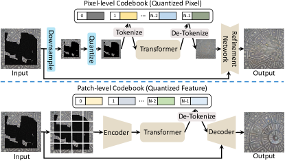
Figure 1: Top: Existing transformer based methods [53]. The output is produced by ICT [53]. Bottom: Our transformer based method. “Tokenize” here means getting the indices of quantized pixels or features, and “De-Tokenize” is the inverse operation.

Recently, transformers have demonstrated their power in various vision tasks [5, 14, 9, 7, 6, 17, 40, 8, 54], thanks to their capability of modeling long-term relationship. Some recent works [53] also attempt to apply transformers for pluralistic image inpainting, and have achieved remarkable success in better diversity and large region inpainting quality. As shown in the top row of Figure 1, they follow the similar design: 1) Downsample the input image into lower resolutions and quantize the pixels; 2) Use the transformer to recover the masked pixels by regarding each quantized pixel as the token; 3) Upsample and refine the low-resolution result by feeding it together with the original input image into an extra CNN network.

In this paper, we argue that using the above pixel-based token makes existing transformer based solutions suffer from the information loss issue from two aspects: 1) “Low resolution”. To avoid high computation complexity of transformer, the input image is downsampled into much lower resolution to reduce the input token number, which not only incurs information loss but also introduces misalignment for the boundaries of masked regions when upsampled back to the original resolution. 2) “Quantization”. To constrain the prediction within a small space, the huge amount ($256^{3}$, in detail) of RGB pixels are quantized into much less (such as 512) qunatized pixels through clustering. The indices of quantized pixels are used as discrete tokens both for the input and prediction target of transformer. Such practice would further result in the information loss.

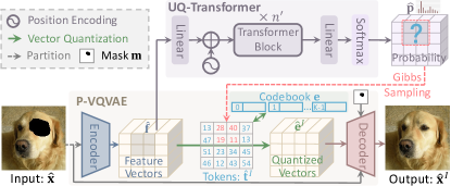
Figure 2: Pipeline of PUT for pluralistic image inpainting. Note that the pluralistic inpainting results are not shown in the figure.

To mitigate these issues, we propose a new transformer based framework PUT, which can reduce the information loss as much as possible. As shown in the bottom row of Figure 1, the original high-resolution input image is directly fed into a patch based encoder without any downsampling and the transformer directly takes the features from the encoder as input without any quantization. Specifically, PUT contains two key designs: Patch-based Vector Quantized Variational Auto-Encoder (“P-VQVAE”, Section 3.1) and Un-Quantized Transformer(“UQ-Transformer”, Section 3.2). P-VQVAE is a specially designed patch auto-encoder: 1) Its encoder converts each image patch into the latent feature in a non-overlapped way, where the non-overlapped design is to avoid the disturbance between masked regions and unmasked regions; 2) As the prediction space of UQ-Transformer, a dual-codebook is built for patch feature tokenization, where masked patches and unmasked patches are separately represented by different codebooks; 3) The decoder in P-VQVAE not only recovers the masked image regions from the inpainted tokens but also maintains unmasked regions unchanged. For UQ-Transformer, it utilizes the quantized tokens of unmasked patches as the prediction targets for masked patches, but takes the un-quantized feature vectors from the encoder as input. Compared to taking the quantized tokens as input, this design can avoid the information loss and help UQ-Transformer make more accurate predictions.

To demonstrate the superiority, we conduct extensive experiments on FFHQ [27], Places2 [65] and ImageNet [12]. The results show that our method outperforms CNN based pluralistic inpainting methods by a large margin on different evaluation metrics. Benefiting from less information loss, our method also achieves much higher fidelity than existing transformer based solutions, especially for large region inpainting and complex large-scale datasets.

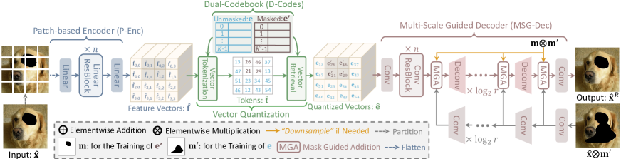
Figure 3: Training procedure of P-VQVAE. The detailed architecture of P-VQVAE could be found in the supplementary material.

2 Related Work

Auto-Encoders. Auto-encoders [23] is a kind of artificial neural network in semi-supervised and unsupervised learning. Among its subclasses, variational auto-encoders (VAE) [29, 13] is widely used for image synthesis tasks [47, 45] as a generative model. It can be trained in self-supervised strategy and generate diverse images through decoder with latent space sampling or autoregressive models [49, 36]. Later, vector quantized variational auto-encoder (VQ-VAE) [48] is proposed for discrete representation learning to circumvent issues of “posterior collaps”, and further developed by VQ-VAE-2 [41]. Recently, based on the similar quantization mechanism with VQ-VAE, VAGAN [17] and dVAE [40] are proposed for conditonal image generation through transformers [50], while PeCo [15] trains a perceptual vision tokenizer for vision transformer BERT-pretraining [55]. Different from previous methods, the proposed “P-VQVAE”, which contains a non-overlapped patch encoder, a dual-codebook and a multi-scale guided decoder, is dedicated for image inpainting.

Visual Transformers. Thanks to the capability of long range relationship modeling, transformers have been widely used in different vision tasks, such as object detection [5, 7], image synthesis [6, 17, 40], object tracking [8, 54] and image inpainting [53]. Specifically, the autoregressive inference mechanism is naturally suitable for image synthesis related tasks, which can bring diverse results while guarantee the quality of the synthesized images [6, 17, 40, 53]. In this paper, we take full advantage of transformer and propose to replace discrete tokens with continuous feature vectors to avoid the information loss.

Image Inpainting. According to the diversity of inpainted images, there are two different types of definition for image inpainting task: deterministic image inpainting and pluralistic image inpainting. Most of the traditional methods, whether diffusion-based methods [3, 16] or path-based methods [2, 20, 11], can only generate single result for each input and may be failed while meeting large-area of missing pixels. Later, some CNN based methods [37, 30, 32, 58, 35, 25] are proposed to ensure consistency of the semantic content of the inpainted images, but still ignore the diversity of results. To generate several diverse results for each masked image, some CNN based [64, 62] and transformer based [53] methods have emerged recently. Among them, transformer based methods [53] show their merits in both quality and diversity than CNN based methods. However, their unreasonable design, like downsampling of input image and quantization of transformer inputs, results in the serious information loss issue. Thus, we propose a novel framework, PUT, which maximizes the input information to achieve better synthesis results.

3 Method

The proposed method mainly consists of a Patch-based Vector Quantized Variational Auto-Encoder (P-VQVAE) and an Un-Quantized transformer (UQ-Transformer). The overview of our method is shown in Figure 2. Let ${\mathbf{x}}\in\mathbb{R}^{H\times W\times 3}$ be an image and ${\mathbf{m}}\in\{0,1\}^{H\times W\times 1}$ be the mask denoting whether a region needs to be inpainted (with value 0) or not (with value 1). $H$ and $W$ are the spatial resolution. The image $\mathbf{\hat{x}}=\mathbf{x}\otimes\mathbf{m}$ is the masked image that contains missing pixels, where $\otimes$ is the elementwise multiplication. The masked image $\mathbf{\hat{x}}$ is first fed into the encoder of P-VQVAE to get the patch based feature vectors. Then UQ-Transformer takes the feature vectors as input and predicts the tokens (i.e., indices) of latent vectors in a codebook for masked regions. Finally, the retrieved latent vectors are used as the quantized vectors for patches and fed into the decoder of P-VQVAE to reconstruct the inpainted image.

3.1 P-VQVAE

To avoid the information loss from input downsampling while maintaining the computation efficiency for the transformer, we utilize the merits of auto-encoder to replace the downsampled pixels with the features from encoder. Compared to the downsampled pixels, the features from encoder can have the same low-resolution for efficiency while contains more information for reconstruction. Considering the task of image inpainting, we specially design P-VQVAE, which contains a patch-based encoder, a dual-codebook and a multi-scale guided decoder.

Patch-based Encoder.

Conventional CNN based encoders process the input image with several convolution kernels in a sliding window manner, which are unsuitable for image inpainting since they would introduce disturbance between masked and unmasked regions. Thus, the encoder of P-VQVAE (denoted as P-Enc) is designed to process input image by several linear layers in a non-overlapped patch manner. Specifically, the masked image $\mathbf{\hat{x}}$ is firstly partitioned into $\frac{H}{r}\times\frac{W}{r}$ non-overlapped patches, where $r$ is the spatial size of patches and is set to 8 by default. For a patch, we call it a masked patch if it contains any missing pixels, otherwise unmasked patch. Each patch is flattened and then mapped into a feature vector. Formally, all feature vectors are denoted as $\mathbf{\hat{f}}=\mathcal{E}(\mathbf{\hat{x}})\in\mathbb{R}^{\frac{H}{r}\times\frac{W}{r}\times C}$, where $C$ (set to 256 by default) is the dimensionality of feature vectors and $\mathcal{E}(\cdot)$ is the encoder function.

Dual-Codebook for Vector Quantization.

Following the works in [48, 41, 17], the feature vectors from encoder are quantized into discrete tokens with the latent vectors in the learnable codebook. By contrast, we design a dual-codebook (denote as D-Codes) for vector quantization, which is more suitable for image inpainting. In D-Codes, the latent vectors are divided into two parts, denoted as $\mathbf{e}\in\mathbb{R}^{K\times C}$ and $\mathbf{e^{\prime}}\in\mathbb{R}^{K^{\prime}\times C}$, which are responsible for feature vectors that mapped from unmasked and masked patches respectively. $K$ and $K^{\prime}$ are the number of latent vectors. Let $\mathbf{m}^{\downarrow}\in\{0,1\}^{\frac{H}{r}\times\frac{W}{r}\times 1}$ be the indicator mask that indicates whether a patch is a masked (with value 0) or unmasked (with value 1) patch. The feature vector $\mathbf{\hat{f}}_{i,j}$ is quantized as:

$$\begin{cases}\mathbf{e}_{k}\ {\rm where}\ k={\rm argmin}_{l}\parallel\mathbf{\hat{f}}_{i,j}\ominus\mathbf{e}_{l}\parallel_{2},\ {\rm if}\ \mathbf{m}^{\downarrow}_{i,j}=1,\\ \mathbf{e^{\prime}}_{k^{\prime}}\ {\rm where}\ k^{\prime}={\rm argmin}_{l}\parallel\mathbf{\hat{f}}_{i,j}\ominus\mathbf{e^{\prime}}_{l}\parallel_{2},\ {\rm else},\end{cases}$$ (1)

where $\ominus$ denotes the operation of elementwise subtraction. Let $\mathbf{\hat{e}}\in\mathbb{R}^{\frac{H}{r}\times\frac{W}{r}\times C}$ and $\mathbf{\hat{t}}=\mathcal{I}(\mathbf{\hat{f}},\mathbf{e},\mathbf{e^{\prime}},\mathbf{m}^{\downarrow})\in\mathbb{N}^{\frac{H}{r}\times\frac{W}{r}}$ be the quantized vectors and tokens for $\mathbf{\hat{f}}$, where $\mathcal{I}(\cdot,\cdot,\cdot,\cdot)$ denotes the function that gets tokens for its first argument and it can be simply implemented by getting the indices of all quantized vectors in $\mathbf{\hat{e}}$. The dual-codebook helps P-Enc learn more discriminative feature vectors for masked and unmasked patches since they are quantized and represented with different codebooks, which further disenchants transformer about the masked and unmasked patches to predict more reasonable results for masked patches.

Multi-Scale Guided Decoder.

For image inpainting task, an indisputable fact is that the unmasked regions should be kept unchanged. To this end, we design a multi-scale guided decoder, denoted as MSG-Dec, to construct the inpainted image $\mathbf{\hat{x}}^{I}$ by referencing the input masked image $\mathbf{\hat{x}}$. Let $\mathbf{\hat{t}}^{I}$ be the inapinted tokens by transformer (Ref. Figure 2 and Section 3.3) and $\mathbf{\hat{e}}^{I}$ be the retrieved quantized vectors from codebook based on $\mathbf{\hat{t}}^{I}$. The construction procedure is formulated as:

$$\mathbf{\hat{x}}^{I}=\mathcal{D}(\mathbf{\hat{e}}^{I},\mathbf{m},\mathbf{\hat{x}}),$$ (2)

where $\mathcal{D}(\cdot,\cdot,\cdot)$ is the decoder function. The decoder consists of two branches: a main branch which starts with the quantized vectors $\mathbf{\hat{e}}^{I}$ and uses several deconvolution layers to generate inpainted images and a reference branch which extracts multi-scale feature maps (with spatial sizes $\frac{H}{2^{l}}\times\frac{W}{2^{l}}$, $0\leq l\leq{\rm log_{2}}r$) from the masked image $\mathbf{\hat{x}}$. The features from the reference branch are fused to the features with the same scale from the main branch through a Mask Guided Addition (MGA) module as:

$$\mathbf{\hat{e}}^{I,l-1}={\rm Deconv}((1-\mathbf{m}^{\downarrow,l})\otimes\mathbf{\hat{e}}^{I,l}+\mathbf{m}^{\downarrow,l}\otimes\mathbf{\hat{f}}^{R,l}),$$ (3)

where $\mathbf{\hat{e}}^{I,l}$ and $\mathbf{\hat{f}}^{R,l}$ are the features with spatial size $\frac{H}{2^{l}}\times\frac{W}{2^{l}}$ from the main branch and the reference branch respectively. $\mathbf{m}^{\downarrow,l}$ is the indicator mask obtained from $\mathbf{m}$ for corresponding spatial size.

Training of P-VQVAE.

To avoid the decoder learning to reconstruct input image $\mathbf{\hat{x}}$ only from the reference image, we get the reference image by randomly erasing some pixels in $\mathbf{\hat{x}}$ with another mask $\mathbf{m^{\prime}}$ (see in Figure 3). Let $\mathbf{\hat{x}}^{R}=\mathcal{D}(\mathbf{\hat{e}},\mathbf{m}\otimes\mathbf{m^{\prime}},\mathbf{\hat{x}}\otimes\mathbf{m^{\prime}})$ be the reconstructed image. In our design, the unmasked pixels in the reference image will be utilized to recover the corresponding pixels in $\mathbf{\hat{x}}^{R}$, while the latent vectors in codebook $\mathbf{e}^{\prime}$ and $\mathbf{e}$ will be used to recover the pixels in $\mathbf{\hat{x}}^{R}$ masked by $\mathbf{m}$ and the remaining pixels respectively. The loss for training P-VQVAE is:

$$L_{vae}=\mathcal{L}_{rec}(\mathbf{\hat{x}},\mathbf{\hat{x}}^{R})+\parallel{\rm sg}[\mathbf{\hat{f}}]\ominus\mathbf{\hat{e}}\parallel^{2}_{2}+\beta\parallel{\rm sg}[\mathbf{\hat{e}}]\ominus\mathbf{\hat{f}}\parallel^{2}_{2},$$ (4)

where ${\rm sg}[\cdot]$ refers to a stop-gradient operation that blocks gradients from flowing into its argument. $\beta$ is the weight for balance and is set to 0.25. $\mathcal{L}_{rec}(\cdot,\cdot)$ is the function to measure the difference between inputted and reconstructed images, including the L1 loss between the pixel values in two images and the gradients of two images, the adversarial loss[19] obtained by a discriminator network, as well as the perceptual loss [26] and the style loss[18] between the two images. Following [48, 41], the second term in Eq. (6) is replaced by Exponential Moving Average (EMA) to optimize the vectors in D-Codes. More details about the training of P-VQVAE could be found in the supplementary material.

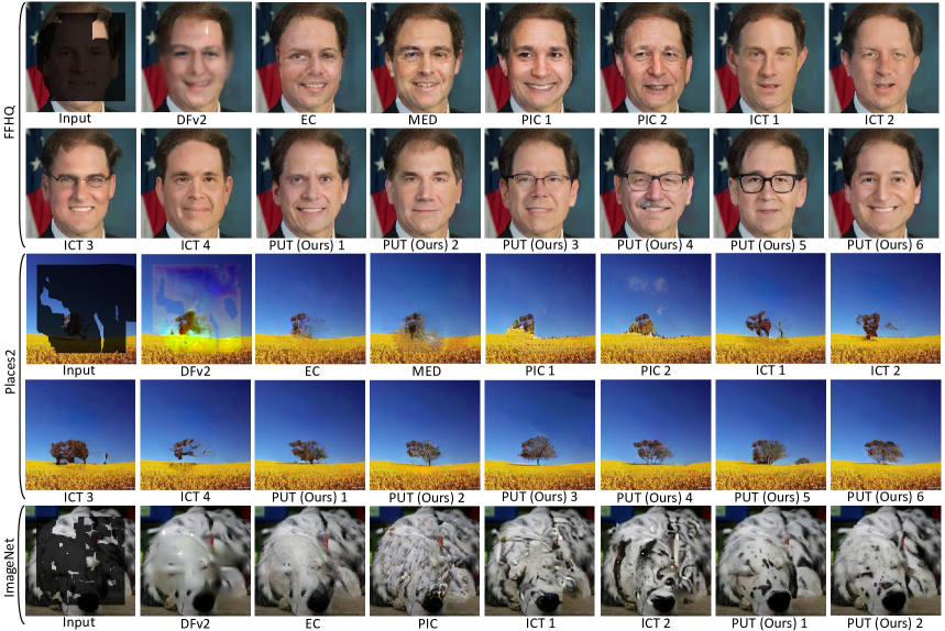
Figure 4: Samples of inpainted results produced by different methods. For PUT, we set $\mathcal{K}=50$. More qualitative comparisons are presented in the supplementary material.

3.2 UQ-Transformer

In existing transformers for image inpainting [53] and synthesis [17, 40], the quantized discrete tokens are used as both the inputs and prediction targets. Given such discrete tokens, transformers suffer from the severe information loss issue, which is harmful to their prediction. In contrast, to take full advantage of feature vectors $\mathbf{\hat{f}}$ from the encoder of P-VQVAE, our UQ-Transformer directly takes them as the inputs and predicts the discrete tokens for masked patches.

Specifically, $\mathbf{\hat{f}}$ is firstly mapped by a linear layer and then added with extra learnable position embeddings for the encoding of spatial information. Finally, following [39], the feature vectors are flattened along spatial dimension to get the final input for the subsequent several transformer blocks. The output of the last transformer block is further projected to the distribution over $K$ latent vectors in codebook $\mathbf{e}$ with a linear layer and a softmax function. We formulate the above procedure as $\mathbf{\hat{p}}=\mathcal{T}(\mathbf{\hat{f}})\in[0,1]^{\frac{H}{r}\times\frac{W}{r}\times K}$, where $\mathcal{T}(\cdot)$ refers the UQ-Transformer function.

Training of UQ-Transformer.

Given a masked image $\mathbf{\hat{x}}$, the distribution of its corresponding inpainted tokens over $K$ latent vectors can be obtained with the pre-trained P-VQVAE and UQ-Transformer $\mathbf{\hat{p}}=\mathcal{T}(\mathcal{E}(\mathbf{\hat{x}}))$. The ground-truth tokens for $\mathbf{x}$ is $\mathbf{t}=\mathcal{I}(\mathcal{E}(\mathbf{x}),\mathbf{e},\mathbf{e^{\prime}},\mathcal{O}(\mathbf{m}^{\downarrow}))$ (Ref. Section 3.1), where $\mathcal{O}(\cdot)$ sets all values in the given argument to 1. UQ-Transformer is trained with cross-entropy loss by fixing P-VQVAE:

$$L_{trans}=\frac{-1}{\sum_{i,j}1-\mathbf{m}_{i,j}^{\downarrow}}\sum_{i,j}(1-\mathbf{m}^{\downarrow}_{i,j}){\rm log}\mathbf{\hat{p}}_{i,j,\mathbf{t}_{i,j}}.$$ (5)

In order to make the training stage consistent with inference stage, where only the quantized vectors can be obtained for masked regions, we randomly quantize the feature vectors in $\mathcal{E}(\mathbf{\hat{x}})$ to the latent vectors in codebook with probability 0.3 before feeding it to UQ-Transformer.

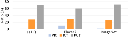
Figure 5: The ratio of each method among the rank 1 images evaluated by human. Statistics are collected from 23 participants.

3.3 Sampling Strategy for Image Inpaining

For the production of diverse results, the tokens for masked patches ($\mathbf{m}_{i,j}^{\downarrow}=0$) are iteratively sampled with Gibbs sampling. Specifically, in each iteration, we first select the patch with the maximum predicted probability among the remaining masked patches. Then the token for the selected patch is sampled from the top-$\mathcal{K}$ predicted elements. Finally, the corresponding latent vector for the sampled token is retrieved to replace the feature vector of the selected patch before feeding UQ-Transformer for the next iteration. After sampling the tokens for all masked patches, we can get all quantized vectors $\mathbf{\hat{e}}^{I}$ with the inpainted tokens $\mathbf{\hat{t}}^{I}$, and the inpainted image can be constructed using Eq. (2). For the production of deterministic results, the tokens for masked patches are sampled with the largest probabilities at once.

4 Experiments

The evaluation is conducted at $256\times 256$ (i.e., $H=256$ and $W=256$) resolution on three different datasets, including FFHQ [27], Places2 [65] and ImageNet [12]. We use the original training and testing splits for Places2 and ImageNet. For FFHQ, we maintain the last 1K images for evaluation and others for training. Following ICT [53], only 1K images are randomly chosen from the test split of ImageNet for evaluation and the irregular masks provided by PConv [30] are used both for training and testing.

((a))

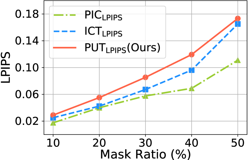
((b))

((c))

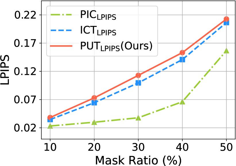
((d))

((e))

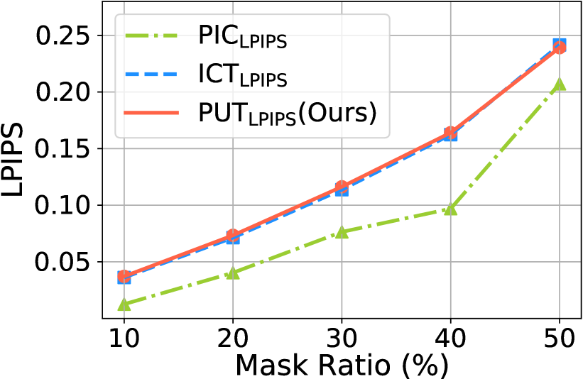
((f))

Figure 6: LPIPS and FID curves with respect to mask ratio on different datasets. For PUT and ICT, $\mathcal{K}=50$.

Dataset		FFHQ [27]			Places2 [65]			ImageNet [12]
Mask Ratio (%)		20-40	40-60	10-60	20-40	40-60	10-60	20-40	40-60	10-60
FID $\downarrow$	DFv2 (ICCV, 2019) [59]	27.344	47.894	30.509	53.107	83.979	59.280	49.900	102.111	64.056
	EC (ICCVW, 2019) [35]	12.949	26.217	16.961	20.180	34.965	23.206	27.821	63.768	39.199
	MED (ECCV, 2020) [31]	13.999	26.252	17.061	28.671	46.815	32.494	40.643	93.983	54.854
	ICTall (ICCV, 2021) [53]	10.442	23.946	15.363	19.309	33.510	23.331	23.889	54.327	32.624
	PUTall (Ours)	11.221	19.934	13.248	19.776	38.206	24.605	19.411	43.239	26.223
	PIC (CVPR, 2019) [64]	22.847	37.762	25.902	31.361	44.289	34.520	49.215	102.561	63.955
	ICT50 (ICCV, 2021) [53]	13.536	23.756	16.202	20.900	33.696	24.138	25.235	55.598	34.247
	PUT50(Ours)	12.784	21.382	14.554	19.617	31.485	22.121	21.272	45.153	27.648
PSNR $\uparrow$	DFv2 (ICCV, 2019) [59]	27.937	22.984	26.783	26.292	22.412	25.391	24.464	20.157	23.387
	EC (ICCVW, 2019) [35]	27.484	22.574	26.181	26.536	22.755	25.975	24.703	20.459	23.596
	MED (ECCV, 2020) [31]	27.117	22.499	26.111	25.401	21.543	24.510	23.730	19.560	22.752
	ICTall (ICCV, 2021) [53]	29.847	23.041	26.736	25.836	22.120	24.986	24.249	20.045	23.317
	PUTall (Ours)	28.356	24.125	27.473	26.580	22.945	25.749	25.721	21.551	24.726
	PIC (CVPR, 2019) [64]	25.157	20.424	24.093	24.073	20.656	23.469	22.921	18.368	21.623
	ICT50 (ICCV, 2021) [53]	26.462	21.816	25.515	24.947	21.126	24.373	23.252	19.025	22.123
	PUT50(Ours)	26.877	22.375	25.943	25.452	21.528	24.492	24.238	19.742	23.264
SSIM$\uparrow$	DFv2 (ICCV, 2019) [59]	0.945	0.850	0.912	0.878	0.741	0.831	0.876	0.719	0.819
	EC (ICCVW, 2019) [35]	0.941	0.826	0.899	0.881	0.734	0.840	0.882	0.714	0.824
	MED (ECCV, 2020) [31]	0.936	0.840	0.903	0.854	0.685	0.796	0.861	0.675	0.795
	ICTall (ICCV, 2021) [53]	0.964	0.863	0.917	0.870	0.723	0.819	0.876	0.711	0.818
	PUTall (Ours)	0.953	0.888	0.908	0.885	0.756	0.840	0.904	0.772	0.838
	PIC (CVPR, 2019) [64]	0.910	0.769	0.865	0.824	0.648	0.775	0.842	0.623	0.766
	ICT50 (ICCV, 2021) [53]	0.931	0.822	0.896	0.850	0.682	0.803	0.852	0.666	0.786
	PUT50(Ours)	0.936	0.845	0.906	0.861	0.703	0.806	0.875	0.704	0.818
MAE$\downarrow$	DFv2 (ICCV, 2019) [59]	0.0187	0.0429	0.0270	0.0230	0.0461	0.0304	0.0303	0.0638	0.0415
	EC (ICCVW, 2019) [35]	0.0177	0.0430	0.0263	0.0207	0.0419	0.0261	0.0271	0.0582	0.0375
	MED (ECCV, 2020) [31]	0.0200	0.0430	0.0277	0.0255	0.0505	0.0336	0.0320	0.0676	0.0434
	ICTall (ICCV, 2021) [53]	0.0129	0.0368	0.0232	0.0221	0.0433	0.0289	0.0362	0.0578	0.0378
	PUTall (Ours)	0.0159	0.0328	0.0213	0.0205	0.0398	0.0269	0.0233	0.0487	0.0321
	PIC (CVPR, 2019) [64]	0.0251	0.0571	0.0350	0.0284	0.0544	0.0353	0.0361	0.0785	0.0509
	ICT50 (ICCV, 2021) [53]	0.0196	0.0445	0.0270	0.0245	0.0487	0.0312	0.0312	0.0677	0.0440
	PUT50(Ours)	0.0191	0.0417	0.0263	0.0235	0.0479	0.0317	0.0281	0.0641	0.0401

Table 1: Quantitative results of different methods. The methods are divided into deterministic and pluralistic groups. The subscript “50” of ICT and PUT is the value of $\mathcal{K}$, while the subscript “all” of ICT and PUT means all tokens are sampled at one iteration.

4.1 Implementation Details

We use P-VQVAE with the same model size and UQ-Transformer with different model sizes for different datasets. The number of latent vectors in dual-codebook (i.e.,$K$ and $K^{{}^{\prime}}$) both are set to 512. The detailed architecture of P-VQVAE and UQ-Transformer could be found in the supplementary material. We train P-VQVAE with batch size 128 and train UQ-Transformer with batch size 48 for FFHQ and 96 for Places2 and ImageNet. The learning rate is warmed up from 0 to 2e-4 and 3e-4 in the the first 5K iterations for P-VQVAE and UQ-Transformer, and then decayed with cosine scheduler. P-VQVAE is optimized with Adam [28] ($\beta_{1}=0,\beta_{2}=0.9$) and UQ-Transformer is optimized with AdamW [33] ($\beta_{1}=0.9$, $\beta_{2}=0.95$). All models are trained to their convergence.

4.2 Main Results

We compare the proposed PUT with the following state-of-the-art inpainting approaches: DeepFillv2 (DFv2) [59], Edge-Connect (EC) [35], MED [31], PIC [64] and ICT [53]. Among them, the last two ones can generate pluralistic results for each input while the others can only produce one deterministic result for the given input. For a fair comparison, we directly use the pre-trained models provided by the authors when available, otherwise train the models by ourselves using the codes and settings provided by the authors.

Qualitative Comparisons.

We first qualitatively compare the inpainted results of different methods in Figure 4. Specifically, DFv2 and EC generally produce blurry images, while the texture of the results generated by MED and PIC contain lots of unnatural artifacts. Compared with ICT, PUT is more powerful in the understanding of global context and maintaining the meaningful textures, as shown in the last row in Figure 4. We argue that the superiority of PUT is mainly due to: 1) high-resolution and 2) un-quantized transformer. Both of them are vital for preserving the information contained in the input images, which are helpful to produce photo-realism images.

User Study.

For the evaluation of subjective quality, the user study is further conducted. Only pluralistic methods are evaluated, including PIC [64], ICT [53]] and PUT. Specifically, we randomly sample 20 pairs of image and mask from the test set of each dataset. For each pair, we generate two inpainted results using each method, and ask the participants to rank these six images according to their photo-realism from high to low. We calculate the ratio of each method among the rank 1 images. Results are shown in Figure 5. Our method takes up at least 60% of the rank 1 images, demonstrating its superiority.

Quantitative Comparisons.

We further demonstrate the superiority of PUT in diversity and fidelity with other pluralistic methods. Specifically, the mean LPIPS distance [61] between pairs of randomly generated results for the same input image is calculated. Following ICT [53], five pairs per input image are generated. Meanwhile, the Fréchet Inception Distance (FID) [22] is also computed between the inpainted images and ground-truth images to reveal the fidelity of generated results. The curves of LPIPS and FID are shown in Figure 6. It can be seen that among the three pluralistic methods, PUT achieves the best fidelity (lowest FID) on all datasets, especially for large area of masked regions and complex scenes (ImageNet [12]). Although PUT and ICT both are implemented with transformers, PUT presents a higher diversity, we owe this to the feeding of original continuous feature vectors without quantization to transformer, which has no information loss issue.

In Table 1, we compare all methods in terms of several metrics, including the peak signal-to-noise (PSNR), structural similarity index (SSIM), relative L1 (MAE) and FID. Only one recovered output is produced for each input. Overall, for pluralistic methods, PUT₅₀ performs the best in almost all metrics on all datasets. Specifically, the FID score of PUT₅₀ on ImageNet with mask ratio 40%-60% is 10.44 lower than that of ICT₅₀. For deterministic methods, PUT_all also achieves almost the best performance. However, the metrics are suitable for the comparison between pluralistic and deterministic methods since diverse and meaningful results can be generated by pluralistic methods.

Dataset	Metric	PUTall (Ours)	CoModGAN [63]	LaMa[44]
FFHQ [27]	PSNR $\uparrow$ / FID $\downarrow$	24.245/21.351	22.430/17.914	-/-
Places2 [65]	PSNR $\uparrow$ / FID $\downarrow$	22.589/38.472	20.962/32.559	22.694/31.160

Table 2: Performance of different methods on FFHQ [27] and Places2 [65] with mask ratio 40%-60% and resolution $512\times 512$.

In Table 2, we further compare PUT_all with LaMa [44] and CoModGAN [63], both of which are recently proposed methods for image inpainting with resolution $512\times 512$. For PUT_all, an upsample network used in ICT [53] is trained to upsample the results from $256\times 256$ to $512\times 512$. As we can see, PUT_all achieves a much better PSNR than CoModGAN, and it is also comparable with LaMa.

Dataset		FFHQ [27]			Places2 [65]
Mask Ratio (%)		20-40	40-60	10-60	20-40	40-60	10-60
FID$\downarrow$	PUTconv	163.610	226.437	173.351	178.057	216.235	179.294
	PUTone	12.112	20.298	13.960	26.015	38.011	28.634
	PUTno_ref	15.014	22.736	16.469	22.821	32.281	25.084
	PUTtok	22.824	38.384	26.098	58.643	120.482	75.625
	PUTqua0	43.621	96.648	54.879	35.127	71.629	44.588
	PUT	12.784	21.382	14.554	19.617	31.485	22.121
PSNR$\uparrow$	PUTconv	12.783	9.735	12.360	12.207	9.347	11.799
	PUTone	26.887	22.335	25.903	24.507	20.571	23.600
	PUTno_ref	26.487	22.249	25.547	25.053	21.398	24.185
	PUTtok	23.916	18.936	22.879	20.940	14.685	19.429
	PUTqua0	24.188	19.564	23.174	24.340	20.239	23.353
	PUT	26.877	22.375	25.943	25.452	21.528	24.492
SSIM$\uparrow$	PUTconv	0.495	0.266	0.445	0.417	0.212	0.373
	PUTone	0.937	0.844	0.906	0.836	0.660	0.776
	PUTno_ref	0.932	0.841	0.901	0.851	0.695	0.798
	PUTtok	0.893	0.745	0.843	0.742	0.453	0.652
	PUTqua0	0.879	0.704	0.820	0.831	0.637	0.763
	PUT	0.945	0.857	0.914	0.861	0.703	0.806
MAE$\downarrow$	PUTconv	0.1420	0.3017	0.1912	0.1447	0.2995	0.1941
	PUT${\rm one}$	0.0191	0.0418	0.0264	0.0256	0.0526	0.0345
	PUTno_ref	0.0202	0.0426	0.0274	0.0249	0.0488	0.0329
	PUTtok	0.0289	0.0689	0.0418	0.0467	0.1337	0.0779
	PUTqua0	0.0281	0.0627	0.0393	0.0269	0.0562	0.0367
	PUT	0.0191	0.0417	0.0263	0.0235	0.0479	0.0317

Table 3: Quantitative results of different methods. All the results are tested with $\mathcal{K}=50$.

4.3 Discussions

Effectiveness of different components.

To show the effectinesess of the patch-based encoder, dual-codebook, multi-scale guided decoder and un-quantized transformer, several methods are designed: 1) PUT^conv means that the patch-based encoder is replaced with a normal CNN encoder, which is implemented with convolution layers; 2) PUT^one refers that there is only one codebook for vector quantization; 3) PUT^no_ref means that there is no reference branch in the decoder; and 4) PUT^tok denotes that the transformer takes the quantized vectors as input rather than the original feature vectors from encoder. In order to show the effectiveness of random quantization of feature vectors while training UQ-Transformer, we further design the fifth model, PUT^qua0, that trains UQ-Transformer without random quantization. For all models, except the modifications mentioned, others remain the same with our default model PUT. Results are shown in Table 3 and Figure 7.

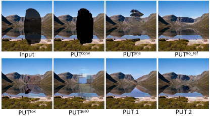
Figure 7: Inpainted results of different models on Places2 [65].

Among all models, PUT^conv performs the worst in all metrics, demonstrating the effectiveness of the non-overlapping patch partition design. Within CNN based encoder, the input images are processed in a sliding window manner, introducing the interaction between masked and unmasked regions, which is fatal to transformer for the prediction of masked regions.

Comparing PUT^one to PUT, the only difference is the training of P-VQVAE with one or two codebooks since the codebook $\mathbf{e^{\prime}}$ is not used in the inference stage. P-VQVAE can learn more discriminative features for masked and unmasked patches with the help of dual-codebook. Interestingly, PUT indeed performs better than PUT^one except the FID score on FFHQ. We speculate that face generation is much easier because all faces share a similar structure. Besides, the facial structure is related with the position in the image since most of the images in FFHQ contain faces in their near-center locations. As we can see in Figure 7, PUT^one sometimes predicts black patches, which is similar to those patches containing missing pixels. Nonetheless, PUT achieves overall better performance than PUT^one.

Compared with PUT, PUT^no_ref constructs the inpainted image without referencing to the input masked image, which leads to a inferior performance in terms of all metrics. For PUT, some useful textures can be recovered with the help of the guidance from the unmasked regions in reference image. As we can see in Figure 7, the result of PUT^no_ref is over smoothed, which is unnatural.

Compared with PUT^tok, PUT performs much better in all metrics. Without quantizing feature vectors to discrete representations, no information contained in the feature will be lost. Such practice helps transformer to understand complex content and maintain the inherit meaningful textures in the input image. However, the training of UQ-Transformer should be carefully designed by randomly quantizing the input feature vectors since only quantized vectors can be obtained for masked regions at the inference stage. The effectiveness of such random quantization during training is obvious while comparing PUT with PUT^qua0.

Misalignment between high and low resolutions.

Existing transformer based methods [53] involves high and low resolutions. The images and masks in high and low resolutions are misaligned, especially the borders of masked regions. For real applications, where the masked regions are often with arbitrary shapes and sizes, such misalignment is non-negligible. In Figure 8, we show one case that with irregular masked regions. We can see that the results of ICT [53] contain lots of artifacts near the misaligned borders. For PUT, the generated results are natural and smooth even though the provided mask is irregular.

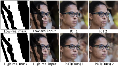
Figure 8: Misalignment between the high and low resolutions. The mask and input image in low-resolution are zoomed in for a better comparison.

5 Conclusions and Limitations

In this paper, we present a novel method, PUT, for pluralistic image inpainting. PUT consists of two main components: 1) patch-based auto-encoder (P-VQVAE) and 2) un-quantized transformer (UQ-Transformer). With the help of P-VQVAE and UQ-Transformer, PUT processes the original high-resolution image without quantization. Such practice preserves the information contained in the input image as much as possible. The main limitation of PUT is the inference speed for the production of diverse results. However, it is a common issue of existing transformer based auto-regressive methods [50, 53, 40, 17]. Two solutions could be adopted to alleviate this limitation: 1) replacing the used transformer block with more efficient ones [24, 56] and 2) sampling tokens for several patches at each iteration. In addition, PUT may be used for editing the contents of images to achieve illicit goals, which can be mitigated using existing synthesized image detectors [57]. Experimental results demonstrate the superiority of PUT, including the fidelity and diversity, especially for large masked regions and complex scenes (such as ImageNet [12]).

Acknowledgement. This work is supported by the National Natural Science Foundation of China (No. 62002336, No. U20B2047) and the Exploration Fund Project of University of Science and Technology of China (YD3480002001).

Supplementary

Appendix A Overview

In this supplementary material, we provide more implementation details, experimental results and analysis, including:

• training of P-VQVAE (Section B).

• sampling strategy for image inpainting ( Section C).

• network architecture of different models (Section D).

• more results on different datasets (Section E).

• more discussions on PUT (Section F), including the inference speed of PUT and some artifacts in inpainted results.

Appendix B Training of P-VQVAE

Given an image $\mathbf{x}$ and two different masks $\mathbf{m}$ and $\mathbf{m^{\prime}}$, the input of P-VQVAE is $\mathbf{\hat{x}}=\mathbf{x}\otimes\mathbf{m}$. The overall loss for the training of P-VQVAE is:

$$L_{vae}=\mathcal{L}_{rec}(\mathbf{\hat{x}},\mathbf{\hat{x}}^{R})+\parallel{\rm sg}[\mathbf{\hat{f}}]\ominus\mathbf{\hat{e}}\parallel^{2}_{2}+\beta\parallel{\rm sg}[\mathbf{\hat{e}}]\ominus\mathbf{\hat{f}}\parallel^{2}_{2},$$ (6)

where $\mathbf{\hat{f}}=\mathcal{E}(\mathbf{\hat{x}})$ denotes the feature vectors extracted by the encoder and $\mathbf{\hat{e}}$ is quantized vectors for $\mathbf{\hat{f}}$. $\mathbf{\hat{x}}^{R}=\mathcal{D}(\mathbf{\hat{e}},\mathbf{m}\otimes\mathbf{m^{\prime}},\mathbf{\hat{x}}\otimes\mathbf{m^{\prime}})$ is the reconstructed image and ${\rm sg}[\cdot]$ refers to a stop-gradient operation that blocks gradients from flowing into its argument.

Input :  $\mathbf{\hat{x}}\in\mathbb{R}^{H\times W\times 3}$: masked image needs to be inpainted
$\mathbf{m}\in\{0,1\}^{H\times W\times 3}$: the mask indicating whether a pixel is masked/missing or not

$\mathcal{K}$: top-$\mathcal{K}$ for Gibbs sampling

Output :  $\mathbf{\hat{x}}^{I}\in\mathbb{R}^{H\times W\times 3}$: the inpainted image

1 Step1: get indicator mask, feature vectors, quantized tokens

2  $\mathbf{m}^{\downarrow}\in\{0,1\}^{\frac{H}{r}\times\frac{W}{r}\times 1}$: calculated from $\mathbf{m}$

3  $\mathbf{\hat{f}}\in\mathbb{R}^{\frac{H}{r}\times\frac{W}{r}\times C}\leftarrow\mathcal{E}(\mathbf{\hat{x}})$

4  $\mathbf{\hat{t}}\in\mathbb{N}^{\frac{H}{r}\times\frac{W}{r}}\leftarrow\mathcal{I}(\mathbf{\hat{f}},\mathbf{e},\mathbf{e^{\prime}},\mathbf{m}^{\downarrow})$ // Sec. 3.1 in the paper

5 $\quad\mathbf{\hat{t}}^{I}\leftarrow\mathbf{\hat{t}}$

6

7Step2: sample tokens for masked patches

8  while $\sum_{i,j}\mathbf{m}^{\downarrow}_{i,j}<\frac{HW}{r^{2}}$ do

9       $\mathbf{\hat{p}}\in[0,1]^{\frac{H}{r}\times\frac{W}{r}\times K}\leftarrow\mathcal{T}(\mathbf{\hat{f}})$ // probabilities, Sec. 3.2 in the paper

10       // select the patch with maximum probability

11       $i^{\prime},j^{\prime}\leftarrow{\rm argmax}_{i,j}(1-\mathbf{m}^{\downarrow}_{i,j})\cdot\max\mathbf{\hat{p}}_{i,j,:}$

12      

13      // sample the token from the top-$\mathcal{K}$ elements in $\mathbf{\hat{p}}_{i^{\prime},j^{\prime},:}$

14       $k\leftarrow\textsc{GibbsSampling}(\mathbf{\hat{p}}_{i^{\prime},j^{\prime},:},\mathcal{K})$

15      

16      // update some variables

17       $\mathbf{\hat{t}}^{I}_{i^{\prime},j^{\prime}}\leftarrow k$, $\mathbf{m}^{\downarrow}_{i^{\prime},j^{\prime}}\leftarrow 1$, $\mathbf{\hat{f}}_{i^{\prime},j^{\prime}}\leftarrow\mathbf{e}_{k}$

18      

19Step3: reconstruct the image

20  $\mathbf{\hat{e}}^{I}\in\leftarrow\textsc{VectorRetrieval}(\mathbf{\hat{t}}^{I},\mathbf{e})$

21  $\mathbf{\hat{x}}^{I}\leftarrow\mathcal{D}(\mathbf{\hat{e}}^{I},\mathbf{m},\mathbf{\hat{x}})$

Return $\mathbf{\hat{x}}^{I}$

Algorithm 1 Sampling Strategy for Pluralistic Image Inpainting

The last term in Eq. (6) is the so-called commitment loss [48] with weighting factor $\beta=0.25$. It is responsible for passing gradient information from decoder to encoder. The second term in Eq. (6) is the codebook loss for the optimization of latent vectors. Following previous works in [48, 41], we replace the second term with the Exponential Moving Average (EMA) to optimize $\mathbf{e}$ and $\mathbf{e^{\prime}}$. Specifically, at each iteration $t$, the latent vector $\mathbf{e}_{k}$ is updated as:

$$\begin{cases}n_{k}^{t}=n_{k}^{t-1}*\gamma+n_{k}*(1-\gamma),\\ \mathbf{\bar{e}}_{k}^{t}=\mathbf{\bar{e}}_{k}^{t-1}*\gamma+\sum\limits_{j}^{n_{k}}(\mathbf{\hat{f}}^{k})_{j}*(1-\gamma),\\ \mathbf{e}^{t}_{k}=\frac{\mathbf{\bar{e}}_{k}^{t}}{n_{k}^{t}},\end{cases}$$ (7)

where $\mathbf{\hat{f}}^{k}$ denotes the set of feature vectors in $\mathbf{\hat{f}}$ that assigned to $\mathbf{e}_{k}$ and $n_{k}$ is the number of feature vectors in $\mathbf{\hat{f}}^{k}$. $\gamma$ is the decay parameter with the value between 0 and 1. We set $\gamma=0.99$ in all our experiments.

The first term in Eq. (6) is the reconstruction loss and $\mathcal{L}_{rec}(\cdot,\cdot)$ is the function to get the difference between the inputted and reconstructed images. It consists of five parts, including L1 loss between the pixel values in two images (denoted as $\mathcal{L}_{pixel}$) and the gradients of two images (denoted as $\mathcal{L}_{grad}$), the adversarial loss [19] $\mathcal{L}_{adv}$, as well as the perceptual loss [26] $\mathcal{L}_{perc}$ and style loss[18] $\mathcal{L}_{style}$ between the two images. The design of the last three losses are inspired by the work in [35]. In the following, we describe the aforementioned losses in detail. Among them:

$$\mathcal{L}_{pixel}=\mathcal{M}(|\mathbf{\hat{x}}\ominus\mathbf{\hat{x}}^{R}|),$$ (8)

$$\mathcal{L}_{grad}=\mathcal{M}(|{\rm grad}[\mathbf{\hat{x}}]\ominus{\rm grad}[\mathbf{\hat{x}}^{R}]|),$$ (9)

where $\mathcal{M}(\cdot)$ refers to a mean-value operation, ${\rm grad}[\cdot]$ is the function calculating the gradient of the given image.

Module	Layer	Parameter size / Stride	Output size
P-Enc	Linear	$192\times 256$	$32\times 32\times 256$
	Linear ResBlock	$\left(\begin{array}[]{c}256\times 128\\ 128\times 256\\ \end{array}\right)\times 8$	$32\times 32\times 256$
	Linear	$256\times 256$	$32\times 32\times 256$
D-Codes	$\mathbf{e}$	$512\times 256$	-
	$\mathbf{e^{\prime}}$	$512\times 256$	-
MSG-Dec	Conv	$256\times 3\times 3\times 256/1$	$32\times 32\times 256$
	Conv ResBlock	$\left(\begin{array}[]{c}256\times 3\times 3\times 128/1\\ 128\times 3\times 3\times 256/1\\ \end{array}\right)\times 8$	$32\times 32\times 256$
	Deconv (Conv)	$256\times 4\times 4\times 256/2$ ($256\times 4\times 4\times 256/2$)	$64\times 64\times 256$ ($32\times 32\times 256$)
	Deconv (Conv)	$256\times 4\times 4\times 128/2$ ($128\times 4\times 4\times 256/2$)	$128\times 128\times 128$ ($64\times 64\times 256$)
	Deconv (Conv)	$128\times 4\times 4\times 64/2$ ($64\times 4\times 4\times 128/2$)	$256\times 256\times 64$ ($128\times 128\times 128$)
	Conv† (Conv)	$64\times 3\times 3\times 3/1$ ($3\times 3\times 3\times 64/1$)	$256\times 256\times 3$ ($256\times 256\times 64$)

Table 4: Architecture of P-VQVAE. For MSG-Dec, the bracketed layers in the bottom four rows denotes the layers in reference branch. Except the convolution layer marked by ${\dagger}$, all the other layers are followed by a ReLU [34] activation function. The structure of Linear and Conv ResBlocks are shown in Figure 9.

Module	Layer	Parameter size / Stride	Output size
Conv-Enc	Conv	$3\times 4\times 4\times 64/2$	$128\times 128\times 64$
	Conv	$64\times 4\times 4\times 128/2$	$64\times 64\times 128$
	Conv	$128\times 4\times 4\times 256/2$	$32\times 32\times 256$
	Conv ResBlock	$\left(\begin{array}[]{c}256\times 3\times 3\times 128/1\\ 128\times 3\times 3\times 256/1\\ \end{array}\right)\times 8$	$32\times 32\times 256$
	Conv	$256\times 3\times 3\times 256$	$32\times 32\times 256$

Table 5: Architecture of the encoder in P-VQVAE^conv. The learnable codebook and decoder are the same with those in P-VQVAE in Table 4. All layers are followed by a ReLU [34] activation function.

The adversarial loss $\mathcal{L}_{adv}$ is computed with the help of a discriminator network $\mathcal{D}_{adv}(\cdot)$:

$$\mathcal{L}_{adv}=-\mathcal{M}({\rm log}[1\ominus\mathcal{D}_{adv}(\mathbf{\hat{x}}^{R})])-\mathcal{M}({\rm log}[\mathcal{D}_{adv}(\mathbf{\hat{x}})]),$$ (10)

where ${\rm log}[\cdot]$ denotes element-wise logarithm operation. The architecture of the discriminator network is the same with that in [35].

The conceptual loss $\mathcal{L}_{perc}$ and style loss $\mathcal{L}_{style}$ are computed based on the activation maps from VGG-19 [42]:

$$\mathcal{L}_{perc}=\sum\limits_{l}^{L_{perc}}\mathcal{M}(|\phi_{l}(\mathbf{\hat{x}})\ominus\phi_{l}(\mathbf{\hat{x}}^{R})|)$$ (11)

$$\mathcal{L}_{style}=\sum\limits_{l}^{L_{style}}\mathcal{M}(|\mathcal{G}(\phi_{l}(\mathbf{\hat{x}}))\ominus\mathcal{G}(\phi_{l}(\mathbf{\hat{x}}^{R}))|)$$ (12)

where $\phi_{l}(\cdot)$ corresponds to different layers in VGG-19 [42], $\mathcal{G}(\cdot)$ denotes the function that gets the Gram matrix of its argument. For $\mathcal{L}_{perc}$ and $\mathcal{L}_{style}$, we set $L_{perc}=\{{\rm relu1\_1},{\rm relu2\_1},{\rm relu3\_1},{\rm relu4\_1},{\rm relu5\_1}\}$ and $L_{perc}=\{{\rm relu2\_2},{\rm relu3\_4},{\rm relu4\_4},{\rm relu5\_2}\}$. The overall reconstruction loss is:

$$\mathcal{L}_{rec} =\mathcal{L}_{pixel}+\lambda_{g}\mathcal{L}_{grad}+\lambda_{a}\mathcal{L}_{adv}$$ (13)

$$+\lambda_{p}\mathcal{L}_{perc}+\lambda_{s}\mathcal{L}_{style}$$

In our implementation, we set $\lambda_{g}=5$, $\lambda_{a}=0.1$, $\lambda_{p}=0.1$ and $\lambda_{s}=250$.

Appendix C Sampling Strategy for Image Inpainting

The overall procedure can be divided into three steps: 1) get the feature vectors $\mathbf{\hat{f}}$ from the masked image $\mathbf{\hat{x}}$ using encoder and get the tokens $\mathbf{\hat{t}}$ by quantizing $\mathbf{\hat{f}}$ with latent vectors in dual-codebook. The tokens for masked patches are not required; 2) get the tokens for masked patches using transformer. Note that the tokens are iteratively sampled with Gibbs sampling following previous transformer-based works [39, 40, 17]; 3) retrieve quantized vectors $\mathbf{\hat{e}}^{I}$ from codebook $\mathbf{e}$ based on the tokens and reconstruct the inpainted image $\mathbf{\hat{x}}^{I}$ using decoder by referencing to masked image $\mathbf{\hat{x}}$. The detailed sampling strategy is shown in Algorithm 1.

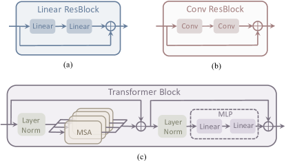
Figure 9: Architecture of different blocks. For Linear and Conv ResBlocks, each layer is followed by a ReLU [34] activation function. For transformer block, there is a GELU [21] activation function between the two linear layers. MSA: Multi-head Self-Attention. MLP: Multi-Layer Perceptron.

Dataset	$n^{\prime}$	$h$	$D$	$D^{\prime}$	Param.
FFHQ [27]	30	8	512	64	95.0M
Places2 [65]	35	8	512	64	110.7M
ImageNet [12]	35	8	1024	128	441.7M

Table 6: UQ-Transformer with different model sizes for different datasets. $n^{\prime}$ and $h$ are the number of transformer block and attention head. $D$ is the dimensionality of feature vectors that before and after each transformer block. $D^{\prime}$ is the dimensionality of feature vector in each attention head.

Appendix D Network Architecture

D.1 Auto-Encoder

For different datasets, we use P-VQVAE with the same model size, and the architecture of our default P-VQVAE is shown in Table 4. The structure of Linear and Conv ResBlocks are shown in Figure 9 (a) and (b). In the paper, Section 4.3, several models are designed to show the effectiveness of different components in our method, including PUT^conv, PUT^one, PUT^no_ref, PUT^qua0 and PUT^tok. The auto-encoders in the last two models are the same with our default P-VQVAE. However, the auto-encoders in PUT^conv , PUT^one and PUT^no_ref are different. For the auto-encoder in PUT^conv (denoted as P-VQVAE^conv), all the linear layers in the encoder are replaced with convolution layers, and the input image is processed in a sliding window manner. Other modules in P-VQVAE^conv are the same with those in P-VQVAE. The architecture of encoder in P-VQVAE^conv (denoted as Conv-Enc) is shown in Table 5. The architecture of the auto-encoder in PUT^one is the same with P-VQVAE, except only one codebook $\mathbf{e}$ is used for training and testing. While for the auto-encdoer in PUT^no_ref, it can be obtained from P-VQVAE by removing the reference branch in decoder.

D.2 Transformer

The architecture of transformer block is depicted in Figure 9 (c). There are several (denoted as $n^{\prime}$) successive transformer blocks in UQ-Transformer. Within each transformer block, the input features will be enhanced by self-attention. Formally, let $\mathbf{\bar{f}}\in\mathbb{R}^{\frac{HW}{r^{2}}\times D}$ be the input of transformer block. At the $b$-th transformer block, the feature vectors are processed as:

$$\mathbf{\tilde{f}}^{b-1} =\mathbf{\bar{f}}^{b-1}+{\rm MSA}({\rm{LN}(\mathbf{\bar{f}}^{b-1})}),$$ (14)

$$\mathbf{\bar{f}}^{b} =\mathbf{\tilde{f}}^{b-1}+{\rm MLP}({\rm LN}(\mathbf{\tilde{f}}^{b-1})),$$

where ${\rm LN}(\cdot)$, ${\rm MLP}(\cdot)$, ${\rm MSA}(\cdot)$ denote layer normalization [1], multi-layer perceptron and multi-head self-attention respectively. More specifically, given input $\mathbf{f}\in\mathbb{R}^{\frac{HW}{r^{2}}\times D}$, ${\rm MSA}(\cdot)$ could be formated as:

$$\mathbf{h}_{j} ={\rm softmax}(\frac{(\mathbf{fw}_{\rm q}^{j})(\mathbf{fw}_{\rm k}^{j})^{T}}{\sqrt{D^{\prime}}})(\mathbf{fw}_{\rm v}^{j}),$$ (15)

$${\rm MSA}(\mathbf{f}) =[\mathbf{h}_{0};\mathbf{h}_{1};...;\mathbf{h}_{h-1}]\mathbf{w}_{\rm o},$$

where $h$ is the number of head, $\mathbf{w}_{\rm q}^{j},\mathbf{w}_{\rm k}^{j},\mathbf{w}_{\rm v}^{j}\in\mathbb{R}^{D\times D^{\prime}}$, $\mathbf{w}_{\rm o}\in\mathbb{R}^{hD^{\prime}\times D}$ are the learnable parameters. $[\cdot;...;\cdot]$ is the operation that concatenates the given arguments along the last dimension. By changing the values of $h,D,D^{\prime}$ and $n^{\prime}$, we can easily scale the size of UQ-Transformer.

We use UQ-Transformer with different model sizes for different datasets, which are shown in Table 6. As a reminder, the configuration of transformers are the same with those in ICT [53].

Appendix E More Results

We show more qualitative comparisons for FFHQ [27] ( Figure 11), Places2 [65] ( Figure 12) and ImageNet [12] (Figure 13 and Figure 14).

	FFHQ [27]	Places2 [65]	ImageNet [12]
UQ-Transformer (# tokens/second)	37.138	32.048	17.186
P-VQVAE (# images/second)	62.949

Table 7: Inference speed of different models. Tested on RTX 3090. The time consumption of P-VQVAE includes extracting feature vectors from image, quantizing feature vectors to latent vectors, and reconstructing the input image.

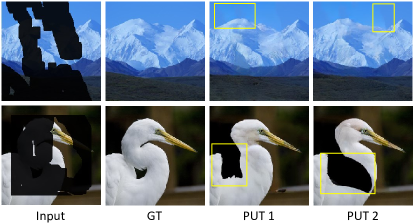
Figure 10: Results with artifacts. Top: color distortion. Bottom: black regions. Please pay attention to the contents in yellow rectangles.

Appendix F More Discussions

Inference speed.

As mentioned in Section 5 in the paper, the main limitation of PUT is the inference speed, which is also a common issue of existing transformer-based auto-regressive methods [50, 53, 40, 17]. Here we present the inference speed of PUT in Table 7. Note that the time consumption of inpainting a masked image depends on the area of masked regions.

Artifacts.

We experimentally find that there sometimes contain some artifacts in the generated results of PUT, as shown in Figure 10. These artifacts can be divided into two categories. 1) Color distortion: the color of generated contents my not be consistent with the color of provided contents in the image. 2) Black region: PUT may produce black regions if the provided masked image contain lots of black pixels.

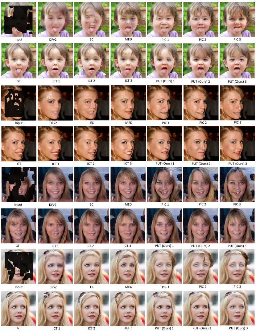
Figure 11: Qualitative comparisons between different methods on FFHQ [27].

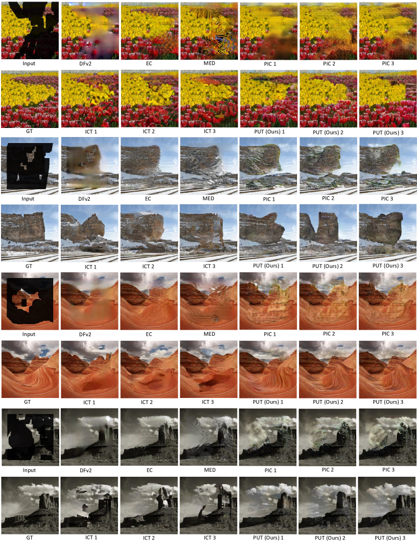
Figure 12: Qualitative comparisons between different methods on Places2 [65].

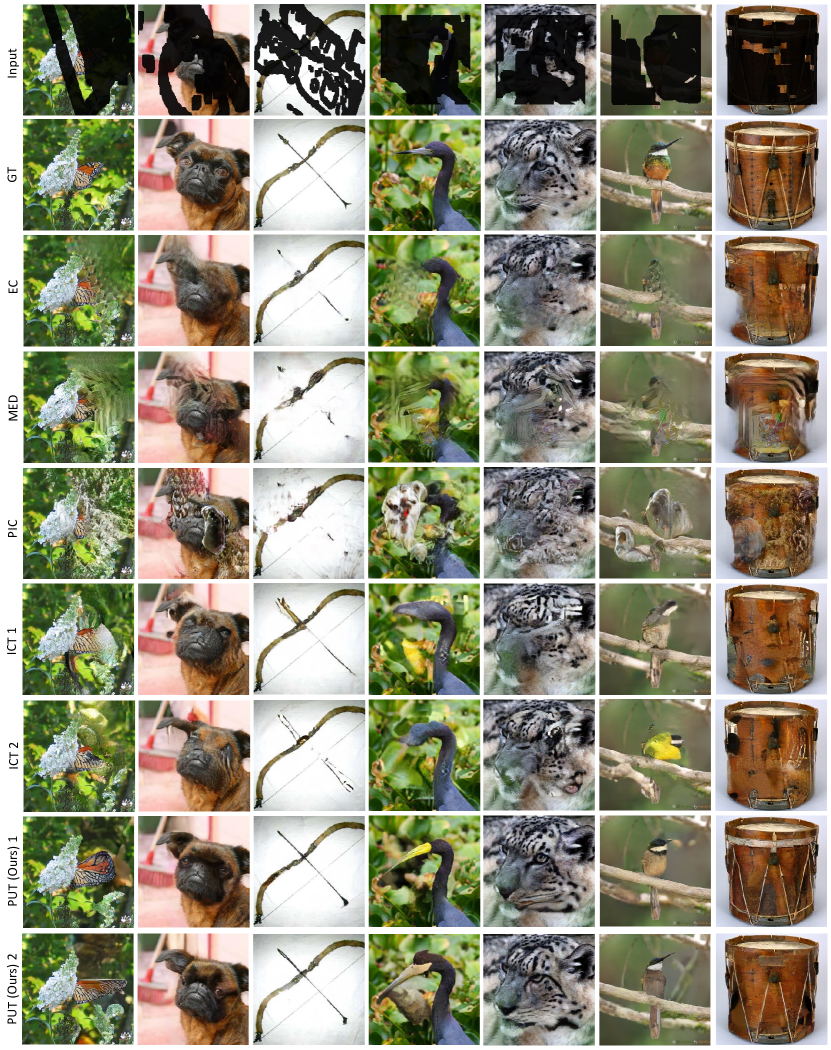
Figure 13: Qualitative comparisons between different methods on ImageNet [12].

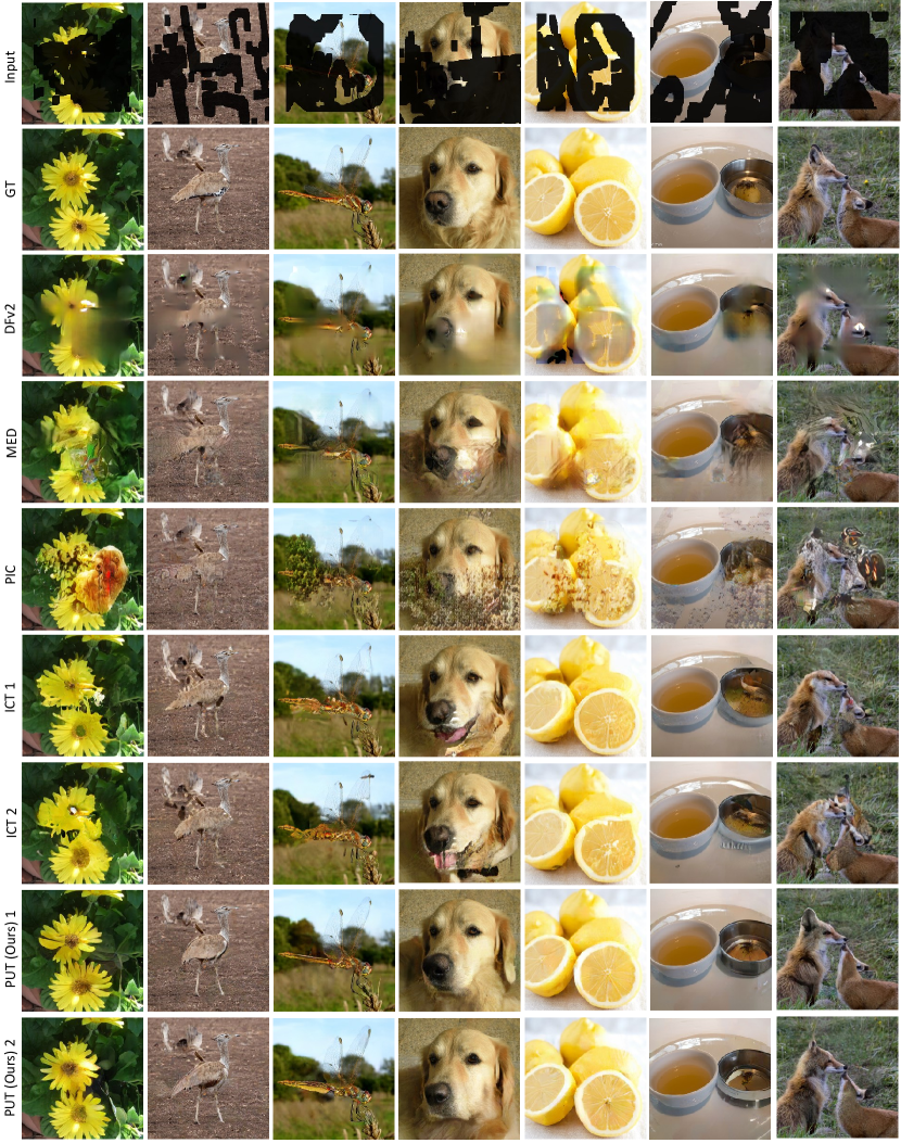
Figure 14: Qualitative comparisons between different methods on ImageNet [12].

References

- [1] Jimmy Lei Ba, Jamie Ryan Kiros, and Geoffrey E Hinton. Layer normalization. arXiv preprint arXiv:1607.06450, 2016.
- [2] Connelly Barnes, Eli Shechtman, Adam Finkelstein, and Dan B Goldman. Patchmatch: A randomized correspondence algorithm for structural image editing. ACM Trans. Graph., 28(3):24, 2009.
- [3] Marcelo Bertalmio, Guillermo Sapiro, Vincent Caselles, and Coloma Ballester. Image inpainting. In Proceedings of the 27th annual conference on Computer graphics and interactive techniques, pages 417–424, 2000.
- [4] Marcelo Bertalmio, Luminita Vese, Guillermo Sapiro, and Stanley Osher. Simultaneous structure and texture image inpainting. IEEE transactions on image processing, 12(8):882–889, 2003.
- [5] Nicolas Carion, Francisco Massa, Gabriel Synnaeve, Nicolas Usunier, Alexander Kirillov, and Sergey Zagoruyko. End-to-end object detection with transformers. In European Conference on Computer Vision, pages 213–229. Springer, 2020.
- [6] Mark Chen, Alec Radford, Rewon Child, Jeffrey Wu, Heewoo Jun, David Luan, and Ilya Sutskever. Generative pretraining from pixels. In International Conference on Machine Learning, pages 1691–1703. PMLR, 2020.
- [7] Ting Chen, Saurabh Saxena, Lala Li, David J Fleet, and Geoffrey Hinton. Pix2seq: A language modeling framework for object detection. arXiv preprint arXiv:2109.10852, 2021.
- [8] Xin Chen, Bin Yan, Jiawen Zhu, Dong Wang, Xiaoyun Yang, and Huchuan Lu. Transformer tracking. In Proceedings of the IEEE/CVF Conference on Computer Vision and Pattern Recognition, pages 8126–8135, 2021.
- [9] Yinpeng Chen, Xiyang Dai, Dongdong Chen, Mengchen Liu, Xiaoyi Dong, Lu Yuan, and Zicheng Liu. Mobile-former: Bridging mobilenet and transformer. In IEEE Conference on Computer Vision and Pattern Recognition (CVPR 2022), 2022.
- [10] Antonio Criminisi, Patrick Pérez, and Kentaro Toyama. Region filling and object removal by exemplar-based image inpainting. IEEE Transactions on image processing, 13(9):1200–1212, 2004.
- [11] Soheil Darabi, Eli Shechtman, Connelly Barnes, Dan B Goldman, and Pradeep Sen. Image melding: Combining inconsistent images using patch-based synthesis. ACM Transactions on graphics (TOG), 31(4):1–10, 2012.
- [12] Jia Deng, Wei Dong, Richard Socher, Li-Jia Li, Kai Li, and Li Fei-Fei. Imagenet: A large-scale hierarchical image database. In 2009 IEEE conference on computer vision and pattern recognition, pages 248–255. Ieee, 2009.
- [13] Carl Doersch. Tutorial on variational autoencoders. arXiv preprint arXiv:1606.05908, 2016.
- [14] Xiaoyi Dong, Jianmin Bao, Dongdong Chen, Weiming Zhang, Nenghai Yu, Lu Yuan, Dong Chen, and Baining Guo. Cswin transformer: A general vision transformer backbone with cross-shaped windows. arXiv preprint arXiv:2107.00652, 2021.
- [15] Xiaoyi Dong, Jianmin Bao, Ting Zhang, Dongdong Chen, Weiming Zhang, Lu Yuan, Dong Chen, Fang Wen, and Nenghai Yu. Peco: Perceptual codebook for bert pre-training of vision transformers. arXiv preprint arXiv:2111.12710, 2021.
- [16] Alexei A Efros and William T Freeman. Image quilting for texture synthesis and transfer. In Proceedings of the 28th annual conference on Computer graphics and interactive techniques, pages 341–346, 2001.
- [17] Patrick Esser, Robin Rombach, and Bjorn Ommer. Taming transformers for high-resolution image synthesis. In Proceedings of the IEEE/CVF Conference on Computer Vision and Pattern Recognition, pages 12873–12883, 2021.
- [18] Leon A Gatys, Alexander S Ecker, and Matthias Bethge. Image style transfer using convolutional neural networks. In Proceedings of the IEEE conference on computer vision and pattern recognition, pages 2414–2423, 2016.
- [19] Ian Goodfellow, Jean Pouget-Abadie, Mehdi Mirza, Bing Xu, David Warde-Farley, Sherjil Ozair, Aaron Courville, and Yoshua Bengio. Generative adversarial nets. Advances in neural information processing systems, 27, 2014.
- [20] James Hays and Alexei A Efros. Scene completion using millions of photographs. ACM Transactions on Graphics (ToG), 26(3):4–es, 2007.
- [21] Dan Hendrycks and Kevin Gimpel. Gaussian error linear units (gelus). arXiv preprint arXiv:1606.08415, 2016.
- [22] Martin Heusel, Hubert Ramsauer, Thomas Unterthiner, Bernhard Nessler, and Sepp Hochreiter. Gans trained by a two time-scale update rule converge to a local nash equilibrium. Advances in neural information processing systems, 30, 2017.
- [23] Geoffrey E Hinton and Richard S Zemel. Autoencoders, minimum description length, and helmholtz free energy. Advances in neural information processing systems, 6:3–10, 1994.
- [24] Jonathan Ho, Nal Kalchbrenner, Dirk Weissenborn, and Tim Salimans. Axial attention in multidimensional transformers. arXiv preprint arXiv:1912.12180, 2019.
- [25] Satoshi Iizuka, Edgar Simo-Serra, and Hiroshi Ishikawa. Globally and locally consistent image completion. ACM Transactions on Graphics (ToG), 36(4):1–14, 2017.
- [26] Justin Johnson, Alexandre Alahi, and Li Fei-Fei. Perceptual losses for real-time style transfer and super-resolution. In European conference on computer vision, pages 694–711. Springer, 2016.
- [27] Tero Karras, Samuli Laine, and Timo Aila. A style-based generator architecture for generative adversarial networks. In Proceedings of the IEEE/CVF Conference on Computer Vision and Pattern Recognition, pages 4401–4410, 2019.
- [28] Diederik P Kingma and Jimmy Ba. Adam: A method for stochastic optimization. arXiv preprint arXiv:1412.6980, 2014.
- [29] Diederik P Kingma and Max Welling. Auto-encoding variational bayes. arXiv preprint arXiv:1312.6114, 2013.
- [30] Guilin Liu, Fitsum A Reda, Kevin J Shih, Ting-Chun Wang, Andrew Tao, and Bryan Catanzaro. Image inpainting for irregular holes using partial convolutions. In Proceedings of the European Conference on Computer Vision (ECCV), pages 85–100, 2018.
- [31] Hongyu Liu, Bin Jiang, Yibing Song, Wei Huang, and Chao Yang. Rethinking image inpainting via a mutual encoder-decoder with feature equalizations. In Computer Vision–ECCV 2020: 16th European Conference, Glasgow, UK, August 23–28, 2020, Proceedings, Part II 16, pages 725–741. Springer, 2020.
- [32] Hongyu Liu, Bin Jiang, Yi Xiao, and Chao Yang. Coherent semantic attention for image inpainting. In Proceedings of the IEEE/CVF International Conference on Computer Vision, pages 4170–4179, 2019.
- [33] Ilya Loshchilov and Frank Hutter. Decoupled weight decay regularization. arXiv preprint arXiv:1711.05101, 2017.
- [34] Vinod Nair and Geoffrey E Hinton. Rectified linear units improve restricted boltzmann machines. In Icml, 2010.
- [35] Kamyar Nazeri, Eric Ng, Tony Joseph, Faisal Qureshi, and Mehran Ebrahimi. Edgeconnect: Structure guided image inpainting using edge prediction. In Proceedings of the IEEE/CVF International Conference on Computer Vision Workshops, pages 0–0, 2019.
- [36] Aäron van den Oord, Nal Kalchbrenner, Oriol Vinyals, Lasse Espeholt, Alex Graves, and Koray Kavukcuoglu. Conditional image generation with pixelcnn decoders. In Proceedings of the 30th International Conference on Neural Information Processing Systems, pages 4797–4805, 2016.
- [37] Deepak Pathak, Philipp Krahenbuhl, Jeff Donahue, Trevor Darrell, and Alexei A Efros. Context encoders: Feature learning by inpainting. In Proceedings of the IEEE conference on computer vision and pattern recognition, pages 2536–2544, 2016.
- [38] Haonan Qiu, Chaowei Xiao, Lei Yang, Xinchen Yan, Honglak Lee, and Bo Li. Semanticadv: Generating adversarial examples via attribute-conditioned image editing. In European Conference on Computer Vision, pages 19–37. Springer, 2020.
- [39] Alec Radford, Jeffrey Wu, Rewon Child, David Luan, Dario Amodei, Ilya Sutskever, et al. Language models are unsupervised multitask learners. OpenAI blog, 1(8):9, 2019.
- [40] Aditya Ramesh, Mikhail Pavlov, Gabriel Goh, Scott Gray, Chelsea Voss, Alec Radford, Mark Chen, and Ilya Sutskever. Zero-shot text-to-image generation. arXiv preprint arXiv:2102.12092, 2021.
- [41] Ali Razavi, Aaron van den Oord, and Oriol Vinyals. Generating diverse high-fidelity images with vq-vae-2. In Advances in neural information processing systems, pages 14866–14876, 2019.
- [42] Karen Simonyan and Andrew Zisserman. Very deep convolutional networks for large-scale image recognition. arXiv preprint arXiv:1409.1556, 2014.
- [43] Yujing Sun, Yizhou Yu, and Wenping Wang. Moiré photo restoration using multiresolution convolutional neural networks. IEEE Transactions on Image Processing, 27(8):4160–4172, 2018.
- [44] Roman Suvorov, Elizaveta Logacheva, Anton Mashikhin, Anastasia Remizova, Arsenii Ashukha, Aleksei Silvestrov, Naejin Kong, Harshith Goka, Kiwoong Park, and Victor Lempitsky. Resolution-robust large mask inpainting with fourier convolutions. In Proceedings of the IEEE/CVF Winter Conference on Applications of Computer Vision, pages 2149–2159, 2022.
- [45] Zhentao Tan, Menglei Chai, Dongdong Chen, Jing Liao, Qi Chu, Bin Liu, Gang Hua, and Nenghai Yu. Diverse semantic image synthesis via probability distribution modeling. In Proceedings of the IEEE/CVF Conference on Computer Vision and Pattern Recognition, pages 7962–7971, 2021.
- [46] Zhentao Tan, Menglei Chai, Dongdong Chen, Jing Liao, Qi Chu, Lu Yuan, Sergey Tulyakov, and Nenghai Yu. Michigan: multi-input-conditioned hair image generation for portrait editing. ACM Transactions on Graphics (TOG), 39(4):95–1, 2020.
- [47] Zhentao Tan, Dongdong Chen, Qi Chu, Menglei Chai, Jing Liao, Mingming He, Lu Yuan, Gang Hua, and Nenghai Yu. Efficient semantic image synthesis via class-adaptive normalization. IEEE Transactions on Pattern Analysis and Machine Intelligence, 2021.
- [48] Aaron van den Oord, Oriol Vinyals, and Koray Kavukcuoglu. Neural discrete representation learning. In Proceedings of the 31st International Conference on Neural Information Processing Systems, pages 6309–6318, 2017.
- [49] Aaron Van Oord, Nal Kalchbrenner, and Koray Kavukcuoglu. Pixel recurrent neural networks. In International Conference on Machine Learning, pages 1747–1756. PMLR, 2016.
- [50] Ashish Vaswani, Noam Shazeer, Niki Parmar, Jakob Uszkoreit, Llion Jones, Aidan N Gomez, Łukasz Kaiser, and Illia Polosukhin. Attention is all you need. In Advances in neural information processing systems, pages 5998–6008, 2017.
- [51] Ziyu Wan, Bo Zhang, Dongdong Chen, Pan Zhang, Dong Chen, Jing Liao, and Fang Wen. Bringing old photos back to life. In proceedings of the IEEE/CVF conference on computer vision and pattern recognition, pages 2747–2757, 2020.
- [52] Ziyu Wan, Bo Zhang, Dongdong Chen, Pan Zhang, Dong Chen, Jing Liao, and Fang Wen. Old photo restoration via deep latent space translation. IEEE Transactions on Pattern Analysis and Machine Intelligence, 2022.
- [53] Ziyu Wan, Jingbo Zhang, Dongdong Chen, and Jing Liao. High-fidelity pluralistic image completion with transformers. In Proceedings of the IEEE/CVF International Conference on Computer Vision, pages 4692–4701, 2021.
- [54] Ning Wang, Wengang Zhou, Jie Wang, and Houqiang Li. Transformer meets tracker: Exploiting temporal context for robust visual tracking. In Proceedings of the IEEE/CVF Conference on Computer Vision and Pattern Recognition, pages 1571–1580, 2021.
- [55] Rui Wang, Dongdong Chen, Zuxuan Wu, Yinpeng Chen, Xiyang Dai, Mengchen Liu, Yu-Gang Jiang, Luowei Zhou, and Lu Yuan. Bevt: Bert pretraining of video transformers. In IEEE Conference on Computer Vision and Pattern Recognition (CVPR 2022), 2022.
- [56] Sinong Wang, Belinda Z Li, Madian Khabsa, Han Fang, and Hao Ma. Linformer: Self-attention with linear complexity. arXiv preprint arXiv:2006.04768, 2020.
- [57] Sheng-Yu Wang, Oliver Wang, Richard Zhang, Andrew Owens, and Alexei A Efros. Cnn-generated images are surprisingly easy to spot… for now. In Proceedings of the IEEE/CVF Conference on Computer Vision and Pattern Recognition, pages 8695–8704, 2020.
- [58] Jiahui Yu, Zhe Lin, Jimei Yang, Xiaohui Shen, Xin Lu, and Thomas S Huang. Generative image inpainting with contextual attention. In Proceedings of the IEEE conference on computer vision and pattern recognition, pages 5505–5514, 2018.
- [59] Jiahui Yu, Zhe Lin, Jimei Yang, Xiaohui Shen, Xin Lu, and Thomas S Huang. Free-form image inpainting with gated convolution. In Proceedings of the IEEE/CVF International Conference on Computer Vision, pages 4471–4480, 2019.
- [60] Xiaohang Zhan, Xingang Pan, Bo Dai, Ziwei Liu, Dahua Lin, and Chen Change Loy. Self-supervised scene de-occlusion. In Proceedings of the IEEE/CVF Conference on Computer Vision and Pattern Recognition, pages 3784–3792, 2020.
- [61] Richard Zhang, Phillip Isola, Alexei A Efros, Eli Shechtman, and Oliver Wang. The unreasonable effectiveness of deep features as a perceptual metric. In Proceedings of the IEEE conference on computer vision and pattern recognition, pages 586–595, 2018.
- [62] Lei Zhao, Qihang Mo, Sihuan Lin, Zhizhong Wang, Zhiwen Zuo, Haibo Chen, Wei Xing, and Dongming Lu. Uctgan: Diverse image inpainting based on unsupervised cross-space translation. In Proceedings of the IEEE/CVF Conference on Computer Vision and Pattern Recognition, pages 5741–5750, 2020.
- [63] Shengyu Zhao, Jonathan Cui, Yilun Sheng, Yue Dong, Xiao Liang, Eric I Chang, and Yan Xu. Large scale image completion via co-modulated generative adversarial networks. In International Conference on Learning Representations (ICLR), 2021.
- [64] Chuanxia Zheng, Tat-Jen Cham, and Jianfei Cai. Pluralistic image completion. In Proceedings of the IEEE/CVF Conference on Computer Vision and Pattern Recognition, pages 1438–1447, 2019.
- [65] Bolei Zhou, Agata Lapedriza, Aditya Khosla, Aude Oliva, and Antonio Torralba. Places: A 10 million image database for scene recognition. IEEE transactions on pattern analysis and machine intelligence, 40(6):1452–1464, 2017.