White-box Testing of NLP models with Mask Neuron Coverage

Abstract

Recent literature has seen growing interest in using black-box strategies like CheckList for testing the behavior of NLP models. Research on white-box testing has developed a number of methods for evaluating how thoroughly the internal behavior of deep models is tested, but they are not applicable to NLP models. We propose a set of white-box testing methods that are customized for transformer-based NLP models. These include mask neuron coverage (mnCover) that measures how thoroughly the attention layers in models are exercised during testing. We show that mnCover can refine testing suites generated by CheckList by substantially reduce them in size, for more than 60% on average, while retaining failing tests – thereby concentrating the fault detection power of the test suite. Further we show how mnCover can be used to guide CheckList input generation, evaluate alternative NLP testing methods, and drive data augmentation to improve accuracy.

White-box Testing of NLP models with Mask Neuron Coverage

Arshdeep Sekhon  and Yangfeng Ji  and Matthew B. Dwyer  and Yanjun Qi University of Virginia, USA

1 Introduction

Previous NLP methods have used black-box testing to discover errors in NLP models. For instance, ChecklistRibeiro et al. (2020) introduces a black-box testing strategy as a new evaluation methodology for comprehensive behavioral testing of NLP models. CheckList introduced different test types, such as prediction invariance in the presence of certain perturbations.

Black-box testing approaches, like Checklist, may produce distinct test inputs that yield very similar internal behavior from an NLP model. Requiring that generated tests are distinct both from a black-box and a white-box perspective – that measures test similarity in terms of latent representations – has the potential to reduce the cost of testing without reducing its error-detection effectiveness. Researchers have explored a range of white-box coverage techniques that focus on neuron activations and demonstrated their benefit on architecturally simple feed-forward networks Pei et al. (2017); Tian et al. (2018); Ma et al. (2018a); Dola et al. (2021). However, transformer-based NLP models incorporate more complex layer types, such as those computing self-attention, to which prior work is inapplicable.

In this paper, we propose a suite of white-box coverage metrics. We first adapt the k-multisection neuron coverage measure from Ma et al. (2018a) to Transformer architectures. Then we design a novel mnCover coverage metric, tailored to NLP models. mnCover focuses on the neural modules that are important for NLP and designs strategies to ensure that those modules’ behavior is thoroughly exercised by a test set. Our proposed coverage metric, when used to guide test generation, can cost-effectively achieve high-levels of coverage.

Figure 1 shows one example of how mnCover can work in concert with CheckList to produce a small and effective test set. The primary insight is that not all text sentences contain new information that will improve our confidence in a target model’s behavior. In this list, multiple sentences were generated with similar syntactic and semantic structure. These sentences cause the activation of sets of attention neurons that have substantial overlap. This represents a form of redundancy in testing an NLP model. Coverage-based filtering seeks to identify when an input’s activation of attention neurons is subsumed by that of prior test inputs – such inputs are filtered. In the Figure the second and third sentences are filtered out because their activation of attention neurons is identical to the first test sentence. As we show in §4 this form of filtering can substantially reduce test suite size while retaining tests that expose failures in modern NLP models, such as BERT.

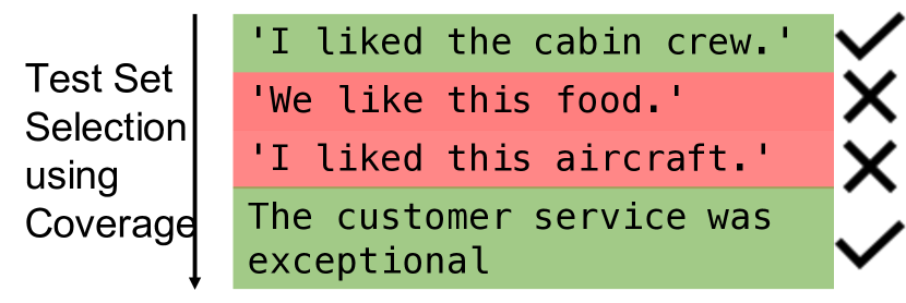
Figure 1: Example of our proposed mnCover’s filtering on a set of test examples.

The primary contributions of the paper lie in:

• Introducing mnCover a test coverage metric designed to address the attention-layers that are characteristic of NLP models and to account for the data distribution by considering task-specific important words and combinations.

• Demonstrating through experiments on 2 NLP models (BERT, Roberta), 2 datasets (SST-2, QQP), and 24 sentence transformations that mnCover can substantially reduce the size of test sets generated by CheckList, by 64% on average, while improving the failure detection of the resulting tests, by 13% on average.

• Demonstrating that mnCover provide an effective supplementary criterion for evaluating the quality of test sets and that it can be used to generate augmented training data that improves model accuracy.

2 Background

Coverage for testing deep networks

The research of Coverage testing focuses on the concept of "adequacy criterion" that defines when “enough” testing has been performed. The white-box coverage testing has been proposed by multiple recent studies to test deep neural networks Pei et al. (2017); Ma et al. (2018a, b); Dola et al. (2021). DeepXplore Pei et al. (2017), a white-box differential testing algorithm, introduced Neuron Coverage for DNNs to guide systematic exploration of DNN’s internal logic. Let us use ${\mathbf{D}}$ to denote a set of test inputs (normally named as a test suite in behavior testing). The Neuron Coverage regarding ${\mathbf{D}}$ is defined as the ratio between the number of unique activated neurons (activated by ${\mathbf{D}}$) and the total number of neurons in that DNN under behavior testing. A neuron is considered to be activated if its output is higher than a threshold value (e.g., 0). Another closely related study, DeepTest Tian et al. (2018), proposed a gray-box, neuron coverage-guided test suite generation strategy. Then, the study DeepGauge Ma et al. (2018a) expands the neuron coverage definition by introducing the kmultisection neuron coverage criteria to produce a multi-granular set of DNN coverage metrics. For a given neuron ${\mathbf{n}}$, the kmultisection neuron coverage measures how thoroughly a given set of test inputs like ${\mathbf{D}}$ covers the range $[low_{n},high_{n}]$. The range $[low_{n},high_{n}]$ is divided into k equal bins (i.e., k-multisections), for $k>0$. For $D$ and the target neuron ${\mathbf{n}}$, its k-multisection neuron coverage is then defined as the ratio of the number of bins covered by $D$ and the total number of bins, i.e., k. For an entire DNN model, the k-multisection neuron coverage is then the ratio of all the activated bins for all its neurons and the total number of bins for all neurons in the DNN.

Transformer architecture

NLP is undergoing a paradigm shift with the rise of large scale Transformer models (e.g., BERT, DALL-E, GPT-3) that are trained on unprecedented data scale and are adaptable to a wide range of downstream tasksBommasani et al. (2021).

These models embrace the Transformer architecture Vaswani et al. (2017) and can capture long-range pairwise or higher-order interactions between input elements. They utilize the self-attention mechanismVaswani et al. (2017) that enables shorter computation paths and provides parallelizable computation for learning to represent a sequential input data, like text. Transformer receives inputs in the general form of word tokens. The sequence of inputs is converted to vector embeddings that get repeatedly re-encoded via the self-attention mechanism. The self-attention can repeat for many layers, with each layer re-encoding and each layer maintaining the same sequence length. At each layer, it corresponds to the following operations to learn encoding of token at position $i$:

$$\alpha^{ij}=\textrm{softmax}\big{(}(\mathbf{W}^{q}\bm{h}_{i})^{\top}(\mathbf{W}^{k}\bm{h}_{j})/\sqrt{\smash[b]{d}}\big{)}$$ (1)

$$\bm{\bar{h}}_{i}=\sum_{j=1}^{M}\alpha^{ij}\mathbf{W}^{v}\bm{h}_{j}$$ (2)

$$\bm{h}^{\prime}_{i}={\sigma}(\bm{\bar{h}}_{i}\mathbf{W}^{r}+\bm{b}_{1})\mathbf{W}^{o}+\bm{b}_{2}.$$ (3)

Here $\mathbf{W}^{k}$ is the key weight matrix, $\mathbf{W}^{q}$ is the query weight matrix,$\mathbf{W}^{v}$ is the value weight matrix, $\mathbf{W}^{r}$ and $\mathbf{W}^{o}$ are transformation matrices, and $\bm{b}_{1}$ and $\bm{b}_{2}$ are bias vectors.

3 Method

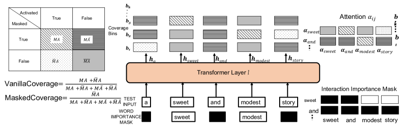
Figure 2: A visual depiction of mnCover for masking neurons to measure coverage.

State-of-the-art NLP models are large-scale with millions of neurons, due to large hidden sizes and multiple layers. We propose to simplify and view these foundation models Bommasani et al. (2021) through two levels of granularity: (1) Word Level: that includes the position-level embeddings at each layer and (2) Pairwise Attention Level: that includes the pairwise self-attention neurons between two positions at each layer. In the rest of this paper, we denote the vector embeddings at location $i$ for layer $l$ as ${{\mathbf{h}}^{\prime}}_{i}^{l}$ and name these as the word level neurons at layer $l$. We also denote the $\alpha^{ij}$ at layer $l$ and head $h$ as $\alpha^{ij}_{lk}$, and call them as the attention level neurons at layer $l$.

3.1 Extending Neuron Coverage (Cover) for Testing NLP Model

Now we use the above two layers’ view we proposed, to adapt the vanilla neuron coverage concepts from the literature to NLP models. First, we introduce a basic definition: "activated neuron bins" Ma et al. (2018b):

Definition 1

Activated Neuron Bins (ANB): For each neuron, we partition the range of its values (obtained from training data) into $B$ bins/sections. We define ANB for a given text input if the input’s activation value from the target neuron falls into the corresponding bin range.

Then we adapt the above definition to the NLP model setting, by using the after-mentioned two layers’ view. We design two phrases: Word Neuron Bins, and Activated Word Neuron Bins in the following  Definition (2).

Definition 2

Activated Word Neuron Bins(AWB): We discretize the possible values of each neuron in $\mathbf{h}^{\prime\ell}_{t}$ (whose $d$-th embedding dimension is $\mathbf{h}^{\prime\ell}_{dt}$) into $B$ sections. We propose a function $\phi_{w}$ who takes two arguments, as $\mathbf{\phi}_{w}(h^{{}^{\prime}lb}_{dt},\mathbf{x})$ for a given input $\mathbf{x}$. $\mathbf{\phi}_{w}(h^{{}^{\prime}lb}_{dt},\mathbf{x})=1$ if it is an activated word neuron bin (shortened as AWB), else $0$ if not activated.

Similarly, for our attention neuron at layer $l$, head $k$, word position $i$ and position $j$: $\alpha_{ij}^{lk}$, we introduce the definition of "attention neuron bins" and "Activated Attention Neuron Bins" in the following Definition (3).

Definition 3

Activated Attention Neuron Bins (AAB): We discretize the possible values of neuron $\alpha_{ij}^{lk}$ into $B$ sections. We denote the state of the $b^{th}$ section of this attention neuron using $\mathbf{\phi}_{a}(\alpha^{ijb}_{lk},\mathbf{x})$. $\mathbf{\phi}_{a}(\alpha^{ijb}_{lk},\mathbf{x})=1$ if it is an activated attention neuron bin (denoted by AAB) by an input $\mathbf{x}$ and $\mathbf{\phi}_{a}(\alpha^{ijb}_{lk},\mathbf{x})=0$ if not activated.

$$\mathbb{N}(\text{\text{AWB}}(\mathbf{x}))=\sum_{ltdb}{\phi}_{w}(h^{{}^{\prime}lb}_{dt},\mathbf{x})$$ (4)

$$\mathbb{N}(\text{AAB}({\mathbf{x}}))=\sum_{ijbk}\mathbf{\phi}_{a}(\alpha^{ijb}_{lk},\mathbf{x})$$ (5)

The coverage, denoted by Cover, of a dataset $\mathcal{T}$ for a target model is then defined as the ratio between the number of “activated" neurons and total neurons:

$$\textsc{Cover}=\dfrac{\mathbb{N}(\text{AWB})+\lambda\mathbb{N}(\text{AAB})}{\mathbb{N}(\text{WB})+\lambda\mathbb{N}(\text{AB})}$$ (6)

Here, $\lambda$ is a scaling factor.

Now let us assume the total number of layers be $D$, total number of heads $H$, maximum length $L$, total bins $B$ and total embedding size be $E$. Considering the example case of the BERTDevlin et al. (2019) model, total number of word level neurons to be measured are then $L\times E\times D=128\times 768\times 13\sim 0.1million$. The total number of the attention level neurons is then $L\times L\times H\times D=128\times 128\times 12\times 12\sim 2million$.

3.2 mask neuron coverage (mnCover)

However, accounting for every word and attention neuron’s behavior for a large pre-trained model like BERT is difficult for two reasons: (1). If we desire to test each neuron at the output of all transformer layers in each BERT layer, we need to account for the behavior of every neuron, which for a large pre-trained model like BERT is in the order of millions.

(2). If we test every possible neuron, we need to track many neurons that are almost irrelevant for a target task and/or model. This type of redundancy makes the behavior testing less confident and much more expensive.

To mitigate these concerns, we propose to only focus on important words and their combinations that may potentially contain ‘surprising’ new information for the model and hence need to be tested.

We assume we have access to a word level importance mask, denoted by $\mathbf{M}_{W}\in\{0,1\}^{|V|}$ and the interaction importance mask by ${\mathbf{M}_{A}}\in\{0,1\}^{|V|\times|V|}$. Each entry in ${\mathbf{M}_{W}}_{w_{t}}\in\{0,1\}$ represents the importance of word $w_{t}$. Similarly, each entry in ${\mathbf{M}_{A}}_{{{\mathbf{x}}_{i},{\mathbf{x}}_{j}}}\in\{0,1\}$ represents the importance of interaction between token $w_{t_{i}}$ and $w_{t_{j}}$. These masks aim for filtering out unimportant tokens (and their corresponding neurons at each layer) for measuring coverage signals. We apply the two masks at each layer to mask out unimportant attention pairs to prevent them from being counted towards coverage calculation. With the masks, the AWB and AAB are revised and we then define mask neuron coverage (mnCover) accordingly:

$$\mathbb{N}(\text{\text{Mask-AWB}}(\mathbf{x}))=\sum_{ltdb}{\mathbb{M}_{w}}_{{\mathbf{x}}_{t}}*{\phi}_{w}(h^{{}^{\prime}lb}_{dt},\mathbf{x})$$

$$\mathbb{N}(\text{\text{Mask-AAB}}(\mathbf{x}))=\sum_{ijkb}{\mathbb{M}_{a}}_{{\mathbf{x}}_{i},{\mathbf{x}}_{j}}*\mathbf{\phi}_{a}(\alpha^{ijb}_{lk},\mathbf{x})$$

$$\textsc{mnCover}=\dfrac{\mathbb{N}(\text{Mask-AWB})+\lambda\mathbb{N}(\text{Mask-AAB})}{\mathbb{N}(\text{WB})+\lambda\mathbb{N}(\text{AB})}\vspace{-5mm}$$ (7)

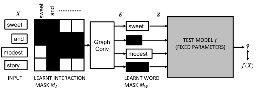
Figure 3: Learning the masks prior to testing: Globally important words and interactions are learnt by masking inputs to a target model.

3.3 Learning Importance Masks

In this section, we explain our mask learning strategy that enables us to learn globally important words and their pairwise combinations for a model’s prediction without modifying a target model’s parameters.

We learn the two masks through a bottleneck strategy, that we call WIMask layer. Given a target model $f$, we insert this mask bottleneck layer between the word embedding layer of a pretrained NLP model and the rest layers of this model. Figure 3 shows a high level overview of the mask bottleneck layer. Using our information bottleneck layer, we learn two masks : (1) a word level mask ${\mathbf{M}_{A}}$, (2) an interaction mask $\mathbf{M}_{W}$.

Learning Word-Pair Interaction Importance Mask: ${\mathbf{M}_{A}}$

The interaction mask aims to discover which words globally interact for a prediction task. We treat words as nodes and represent their interactions as edges in an interaction graph. We represent this unknown graph as a matrix $\mathbf{M}_{A}={\{{\mathbf{M}_{A}}_{ij}\}}_{V\times V}$. Each entry ${\mathbf{M}_{A}}_{{\mathbf{x}}_{i},{\mathbf{x}}_{j}}\in\{0,1\}$ is a binary random variable, such that ${\mathbf{M}_{A}}_{ij}\sim\mathit{Sigmoid}({\mathbf{\lambda}}_{ij})$, follows Bernoulli distribution with parameter $\mathit{Sigmoid}({\mathbf{\lambda}}_{ij})$. ${\mathbf{M}_{A}}_{ij}$ specifies the presence or absence of an interaction between word $i$ and word $j$ in the vocabulary $\mathbb{V}$. Hence, learning the word interaction graph reduces to learning the parameter matrix $\mathbf{\lambda}=\{\mathbf{\lambda}_{ij}\}_{V\times V}$. In Section 3.3.1, we show how $\mathbf{\lambda}$ (and therefore $\mathbf{M}_{A}$) is learned through a variational information bottleneck loss formulation (details in  Section (A.2)).

Based on the learnt interaction mask $\mathbf{M}_{A}$, each word embedding $\mathbf{x}_{i}$ is revised using a graph based summation from its interacting neighbors’ embedding $\mathbf{x}_{j},j\in\mathcal{N}(i)$:

$${\mathbf{e}}_{i}^{\prime}={\mathbf{x}}_{i}+\sigma\Bigg{(}\tfrac{1}{|\mathcal{N}(i)|}\sum_{j\in\mathcal{N}(i)}{\mathbf{x}}_{j}{\mathbf{W}}\Bigg{)}$$ (8)

$\sigma(\cdot)$ is the ReLU non-linear activation function and ${\mathbf{W}}\in\mathbb{R}^{H\times H}$ is a weight matrix. We denote the resulting word representation vector as ${\mathbf{e}}^{\prime}_{i}$. Here $j\in\mathcal{N}(i)$, and $\mathcal{N}(i)$ denotes those neighbor nodes of ${\mathbf{x}}_{i}$ on the graph $\mathbf{M}_{A}$ and in ${\mathbf{x}}$. Eq. (8) is motivated by the design of Graph convolutional networks (GCNs) that were introduced to learn useful node representations that encode both node-level features and relationships between connected nodes Kipf and Welling (2016). Differently in our work, we need to learn the graph $\mathbf{M}_{A}$, through the $\lambda$ parameter. We can compute the simultaneous update of all words in input text ${\mathbf{x}}$ together by concatenating all ${\mathbf{e}}^{\prime}_{i}$. This gives us one matrix $\mathbf{E}^{\prime}\in\mathbf{M}_{W}^{L\times H}$, where $L$ is the length of input and $H$ is the embedding dimension of ${\mathbf{x}}_{i}$.

Learning Word Importance Mask: $\mathbf{M}_{W}$

This word mask aims to learn a global attribution word mask $\mathbf{M}_{W}$. Aiming for better word selection, $\mathbf{M}_{W}$ is designed as a learnable stochastic layer with $\mathbf{M}_{W}\in\{0,1\}^{V}$. Each entry in $\mathbf{M}_{W}$ (e.g., ${\mathbf{M}_{W}}_{w}\in\{0,1\}$ for word $w$) follows a Bernoulli distribution with parameter $p_{w}$. The learning reduces to learning the parameter vector $\mathbf{p}$.

During inference, for an input text ${\mathbf{x}}$, we get a binary vector ${\mathbf{M}_{W}}_{{\mathbf{x}}}$ from $\mathbf{M}_{W}$ that is of size $L$. Its $i$-th entry ${\mathbf{M}_{W}}_{{{\mathbf{x}}}_{i}}\in\{0,1\}$ is a binary random variable associated with the word token at the $i$-th position. ${\mathbf{M}_{W}}_{{\mathbf{x}}}$ denotes how important each word is in an input text ${\mathbf{x}}$. Then we use the following operation (a masking operation) to generate the final representation of the $i$-th word: ${{\mathbf{z}}}_{i}={\mathbf{M}_{W}}_{{\mathbf{x}}_{i}}{{\mathbf{e}}^{\prime}}_{i}$. We then feed the resulting ${\mathbf{Z}}$ to the target model $f$.

3.3.1 Learning Word and Interaction Masks for a target model $f$:

During training, we fix the parameters of target model $f$ and only train the WIMask layerto get two masks.

We learn this trainable layer using the following loss objective, with the derivation of each term explained in the following section:

$$\mathcal{L}({\mathbf{x}},f({\mathbf{x}}),\hat{y})=\ell_{f({\mathbf{x}}),\hat{y}}+\beta_{sparse}\ell_{sparse}\\ +\beta_{i}\ell{prior_{{\mathbf{M}_{W}}_{{\mathbf{x}}}}}+\beta_{g}\ell_{prior_{{\mathbf{M}_{A}}_{{\mathbf{x}}}}}$$ (9)

First, we want to ensure that model predictions with WIMask layer added are consistent with the original prediction $f({\mathbf{x}})$. Hence, we minimize the cross entropy loss ${\ell}_{f({\mathbf{x}}),\hat{y}}$ between $f({\mathbf{x}})$ and the newly predicted output $\hat{y}$ (when with the bottleneck layer).

Then $\ell_{sparse}$ is the sparsity regularization on ${\mathbf{M}_{A}}_{{\mathbf{x}}}$, $\ell{prior_{\mathbf{M}_{W}}}$ is the KL divergence between $\mathbf{M}_{W}$ and a random bernoulli prior. Similarly, $\ell{prior_{{\mathbf{M}_{A}}}}$ is the KL divergence between ${\mathbf{M}_{A}}$ and a random bernoulli prior. We provide detailed derivations in Section  A.2.

4 Experiments

Our experiments are designed to answer the following questions:

1. Will a test set filtered by mnCover find more errors from a SOTA NLP model?

2. Does mnCover achieve test adequacy faster, i.e. achieve higher coverage in fewer samples?

3. Does mnCover help us compare existing testing benchmarks?

4. Can mnCover help us automatically select non-redundant samples for better augmentation?

Datasets and Models

We use pretrained model BERT-baseDevlin et al. (2019) and RoBERTa-baseLiu et al. (2019) provided by Morris et al. (2020) finetuned on SST-2 dataset and Quora Question Pair (QQP) dataset. For the QQP dataset, we use the model finetuned on the MRPC dataset. We train a word level mask ($\mathbf{M}_{W}$) and an interaction mask (${\mathbf{M}_{A}}$) for each of these settings. We use a learning rate of $1e-05$, $\beta_{i}=0.001$, $\beta_{g}=0.001$, and $\beta_{s}=0.001$ for all models.

We have provided the test accuracy of the target models and the models trained with masks in Table 5. Note that the ground truth labels here are the predictions from the target model $f$ without the WIMask layer, as our goal is to ensure fidelity of the WIMask +$f$ to the target model $f$. Table 5 shows that training the WIMask +$f$ model maintains the target model’s predictions $f$ as indicated by higher accuracies.

Test Transformation Name	Failure Rate ($\%$)				Dataset Size Reduction ($\%$)
	D	D+Cover	D+mnCover	$\Delta_{D+\textsc{mnCover}}$	D+Cover	D+mnCover
change names	5.14	${\bf 100.00}_{16.86}$	${\bf 100.00}_{16.86}$	${94.86}_{11.73}$	62.84	62.84
add negative phrases	6.80	${\bf 100.00}_{19.16}$	${\bf 99.34}_{19.16}$	${92.54}_{12.36}$	75.40	75.99
protected: race	68.00	${\bf 100.00}_{73.02}$	${\bf 99.37}_{72.13}$	${31.37}_{4.13}$	44.33	43.54
used to,but now	29.87	${\bf 53.30}_{46.27}$	${\bf 53.30}_{46.75}$	${23.43}_{16.88}$	84.61	84.61
protected: sexual	86.83	${\bf 100.00}_{87.31}$	${\bf 100.00}_{88.99}$	${13.17}_{2.15}$	83.83	86.83
change locations	8.69	${\bf 21.43}_{8.31}$	${\bf 21.43}_{8.31}$	${12.74}_{-0.38}$	86.47	86.93
change neutral words with BERT	9.80	${\bf 20.00}_{13.04}$	${\bf 20.84}_{13.39}$	${11.04}_{3.59}$	73.40	73.88
contractions	2.90	${\bf 5.52}_{3.94}$	${\bf 8.22}_{4.34}$	${5.32}_{1.44}$	34.80	34.80
2 typos	11.60	${\bf 18.00}_{11.14}$	${\bf 16.00}_{10.87}$	${4.40}_{-0.73}$	10.00	10.00
change numbers	3.20	${\bf 7.14}_{3.94}$	${\bf 7.14}_{3.29}$	${3.94}_{0.09}$	87.70	88.44
typos	6.60	${\bf 10.00}_{6.45}$	${\bf 10.00}_{6.24}$	${3.40}_{-0.36}$	10.00	10.00
neutral words in context	96.73	${\bf 100.00}_{96.91}$	${\bf 100.00}_{96.82}$	${3.27}_{0.09}$	21.33	28.50
protected: religion	96.83	${\bf 100.00}_{93.42}$	${\bf 100.00}_{98.02}$	${3.17}_{1.19}$	89.67	89.67
add random urls and handles	15.40	${14.63}_{9.17}$	${\bf 17.86}_{11.56}$	${2.46}_{-3.84}$	87.60	87.60
simple negations: not neutral is still neutral	97.93	${\bf 100.00}_{98.49}$	${\bf 100.00}_{98.34}$	${2.07}_{0.41}$	45.67	46.03
simple negations: not negative	10.40	${\bf 12.00}_{9.56}$	${\bf 12.42}_{9.90}$	${2.02}_{-0.50}$	80.11	80.37
my opinion is what matters	41.53	${\bf 42.49}_{36.79}$	${\bf 43.14}_{36.79}$	${1.61}_{-4.74}$	84.16	84.32
punctuation	5.40	${\bf 6.80}_{5.37}$	${\bf 6.80}_{6.26}$	${1.40}_{0.86}$	10.00	9.11
Q & A: yes	0.40	${\bf 1.33}_{0.50}$	${\bf 1.71}_{0.49}$	${1.31}_{0.09}$	82.33	83.14
Q & A: no	85.20	${\bf 86.33}_{76.42}$	${\bf 86.22}_{77.16}$	${1.02}_{-8.04}$	82.34	83.12
simple negations: negative	6.13	${\bf 7.33}_{5.63}$	${\bf 7.12}_{5.70}$	${0.99}_{-0.44}$	78.63	78.71
reducers	0.13	${\bf 0.27}_{0.10}$	${\bf 1.03}_{0.10}$	${0.90}_{-0.03}$	67.00	66.77
intensifiers	1.33	${1.05}_{0.31}$	${\bf 1.83}_{1.01}$	${0.49}_{-0.33}$	66.65	66.96
Average Improvement	-	$13.51_{1.10}$	$13.78_{1.55}$	$13.78_{1.55}$	$62.99$	$63.57$

Table 1: Failure Rate(%) obtained using BERT model on the original dataset $D$, the dataset filtered using Cover coverage (D+Cover columns) and the dataset filtered with mnCover coverage (D+mnCover columns) from the Sentiment Test Suite. We report both the max failure rate as well as the mean in the subscript across $10$ thresholds of coverage. Rows are sorted regarding the failure rate difference between the dataset filtered using mnCover and the original dataset (column $\Delta_{D+\textsc{mnCover}}$).

Test Transformation Name	Failure Rate ($\%$)				Dataset Size Reduction ($\%$)
	D	D+Cover	D+mnCover	$\Delta_{D+\textsc{mnCover}}$	D+Cover	D+mnCover
Q & A: yes	46.20	${\bf 100.00}_{51.45}$	${\bf 100.00}_{51.45}$	${53.80}_{5.25}$	82.37	81.58
protected: race	61.67	${\bf 100.00}_{66.00}$	${\bf 100.00}_{66.00}$	${38.33}_{4.34}$	44.33	44.33
neutral words in context	80.87	${\bf 100.00}_{83.43}$	${\bf 100.00}_{83.31}$	${19.13}_{2.44}$	21.27	21.39
protected: religion	73.00	${\bf 74.19}_{62.31}$	${\bf 85.71}_{63.64}$	${12.71}_{-9.36}$	89.67	89.67
protected: sexual	91.00	${\bf 100.00}_{84.25}$	${\bf 100.00}_{84.25}$	${9.00}_{-6.75}$	83.83	83.83
simple negations: not neutral is still neutral	91.53	${\bf 100.00}_{92.93}$	${\bf 100.00}_{92.24}$	${8.47}_{0.71}$	45.87	46.11
add negative phrases	29.60	${\bf 36.46}_{23.15}$	${\bf 36.72}_{23.15}$	${7.12}_{-6.45}$	75.40	75.40
Q & A: no	57.53	${\bf 61.67}_{53.60}$	${\bf 62.41}_{53.60}$	${4.87}_{-3.93}$	82.31	82.31
simple negations: not negative	95.40	${\bf 100.00}_{96.11}$	${\bf 100.00}_{95.92}$	${4.60}_{0.52}$	80.14	80.27
2 typos	5.20	${\bf 6.40}_{5.10}$	${\bf 7.33}_{5.33}$	${2.13}_{0.13}$	10.00	10.00
change neutral words with BERT	9.20	${\bf 11.11}_{7.81}$	${\bf 11.11}_{7.48}$	${1.91}_{-1.72}$	73.40	72.45
intensifiers	1.13	${\bf 2.68}_{1.69}$	${\bf 2.68}_{1.87}$	${1.55}_{0.73}$	66.65	66.46
change names	4.53	${\bf 4.88}_{2.57}$	${\bf 5.81}_{2.37}$	${1.28}_{-2.16}$	62.84	62.84
punctuation	4.80	${\bf 6.00}_{4.03}$	${\bf 6.00}_{3.96}$	${1.20}_{-0.84}$	10.00	10.00
change locations	6.16	${\bf 7.32}_{5.28}$	${\bf 7.32}_{4.44}$	${1.16}_{-1.72}$	86.47	87.43
typos	3.00	${\bf 3.60}_{1.90}$	${\bf 4.00}_{2.39}$	${1.00}_{-0.61}$	10.00	10.00
simple negations: negative	1.33	${\bf 2.00}_{1.07}$	${\bf 1.99}_{1.20}$	${0.65}_{-0.13}$	78.63	78.68
used to,but now	52.73	${\bf 53.30}_{46.27}$	${\bf 53.30}_{45.58}$	${0.56}_{-7.16}$	84.61	83.74
my opinion is what matters	56.47	${\bf 59.00}_{50.32}$	${\bf 56.86}_{49.87}$	${0.39}_{-6.60}$	84.20	84.20
contractions	1.00	${\bf 1.37}_{0.74}$	${\bf 1.37}_{0.63}$	${0.37}_{-0.37}$	34.80	34.80
reducers	0.40	${0.34}_{0.14}$	${\bf 0.57}_{0.27}$	${0.17}_{-0.13}$	67.05	66.35
change numbers	2.50	${1.63}_{0.48}$	${2.41}_{0.72}$	${-0.09}_{-1.78}$	87.70	87.70
add random urls and handles	11.40	${8.33}_{5.22}$	${8.65}_{4.55}$	${-2.75}_{-6.85}$	87.60	88.18
Average Improvement	-	$6.68_{-1.10}$	$7.29_{-1.85}$	$7.29_{-1.85}$	$63.01$	$62.95$

Table 2: Failure Rate(%) obtained using RoBERTa model on the original dataset $D$, the dataset filtered using Cover coverage (D+Cover columns) and the dataset filtered with mnCover coverage (D+mnCover columns) from the Sentiment Test Suite. We report both the max failure rate as well as the mean in the subscript across $10$ thresholds of coverage. Rows are sorted regarding the failure rate difference between the dataset filtered using mnCover and the original dataset (column $\Delta_{D+\textsc{mnCover}}$).

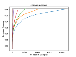
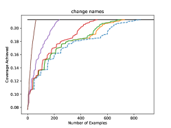
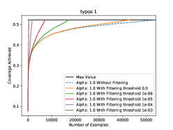
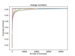
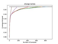
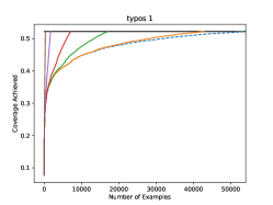
Figure 4: mnCover is able to achieve higher coverage with a fewer number of samples than without coverage based filtering. For this experiment we use the RoBERTa model. In the top row, we do not shuffle the examples and the bottom row with shuffling. Even with a threshold of $0.0$, we are able to significantly reduce the number of samples that achieve the same coverage as the unfiltered set: we are able to achieve an average reduction (across transformations) of 28.83%, 54.06% , 71.48% , 88.67% and 97.17% for $\{0.0,1e-04,1e-03,1e-02,1e-01\}$ thresholds respectively.

4.1 Experiment 1: Removing Redundant Test Inputs during Model Testing

Motivation

CheckList Ribeiro et al. (2020) provides a method to generate a large number of test cases corresponding to a target template. It introduces different transformations that can be used to generate samples to check for a desired behavior/functionality. For example, to check for a model’s behavior w.r.t typos in input texts, it generates examples with typos and queries the target model. CheckList then compares failure rates across models for the generated examples to identify failure modes. However, it does not provide a method to quantify the number of tests that need to be generated or to determine which examples provide the most utility in terms of fault detection. Such a blind generation strategy may suffer from sampling bias and give a false notion of a model’s failure modes.

Setup

We evaluate mnCover’s ability to redundant test samples out of the generated tests for a target model. The different transformations used are summarized in Column I of Table 1,  Table 2, and  Table 6. We measure failure rate on an initial test set of size $N=1500$. We then filter the generated tests based on our mnCover coverage criteria: if adding a test example into a test suite does not lead to an increase in its coverage, it is discarded. We then measure failure rate of the new filtered test set.

Results

In Table 1, we observe that mnCover can select more failure cases for the BERT model across all 23 transformation on SST-2 dataset. On average, both mnCover and Cover can help reduce more than 60% of the test suite size, and mnCover achieves a slight advantage over Cover. In Table 2, when using RoBERTa model, mnCover based filtering wins over the original dataset in 21 of 23 cases. The average improvement of mnCover regarding error detection is 7.29% on RoBERTa model and 13.78% on BERT model. We include similar results on QQP dataset in Table 6.

4.2 Experiment 2: Achieving Higher Dataset Coverage with Fewer Data Points

Motivation

We revisit the question: given a test generation strategy, does adding more test samples necessarily add more information? In this set of experiments, we appeal to the software engineering notion of “coverage" as a metric of test adequacy. We show that we can reach a target level of test adequacy faster, i.e. a higher coverage, hence achieving more rigorous behavior testing, with fewer test examples, by using coverage as an indicator of redundant test samples.

Setup:

We use the training set as seed examples and generate samples using transformations used in the previous experiment listed in Table  1. Similar to the previous set of examples, we disregard an example if the increase in its coverage is below $threshold$. We vary these $threshold$ values $\in\{1e-04,1e-03,1e-02,1e-01,0.0\}$. Higher the $threshold$, more number of examples get filtered out.

Results:

In Figure 4, we show that using our coverage guided filtering strategy, we are able to achieve coverage with a fewer number of samples than without coverage based filtering.

Even with a threshold of $0.0$, we are able to significantly reduce the number of samples that achieve the same coverage as the unfiltered set: we are able to achieve an average reduction across transformations (higher the better) of 71.17%, 45.94%, 28.52%, 11.33% and 2.83% for $\{0.0,1e-04,1e-03,1e-02,1e-01\}$ thresholds respectively.

Test Set	mnCover
A1	0.175
A1 + A2	0.182
A1 + A2 + A3	0.185
A2	0.179
A3	0.181

Table 3: mnCover Values on the Dynabench test sets

4.3 Experiment 3: mnCover as a Metric to Evaluate Testing Benchmarks

Motivation:

In this set of experiments, we utilize coverage as a test/benchmark dataset evaluation measure. Static test suites, such as the GLUE benchmark, saturate and become obsolete as models become more advanced. To mitigate the saturation of static benchmarks with model advancement, Kiela et al. (2021) introduced Dynabench, a dynamic benchmark for Natural Language Inference(NLI). Dynabench introduced a novel human-and-model-in-the-loop dataset, consisting of three rounds that progressively increase in difficulty and complexity. This results in three sets of training, validation and test datasets, with increasing complexity testing datasets. We use mnCover as an additional validation measure for the datasets.

Setup:

We test the ROBERTA-Large model provided by Dynabench trained on training data from all three rounds of the benchmark. We use $10$ as the number of bins and $\lambda=1.0$.

Results:

We measure coverage achieved by each of the test sets individually as well as in combination. We have summarized the results in Table 3. The test sets indeed provide more novel test inputs to the model as indicated by the increasing coverage as the test sets from each split are taken into consideration. The low values arise from a large architecture, (24-layer, 1024-hidden, 16-heads) that is potentially still unexplored with $1000$ samples from each test set.

4.4 Experiment 4: Coverage Guided Augmentation

Motivation:

Data augmentation refers to strategies for increasing the diversity of training examples without explicitly collecting new data. This is usually achieved by transforming training examples using a transformation. A number of automated approaches have been proposed to automatically select these transformations including like Xie et al. (2019). Since computing mnCover does not require retraining, and the input selection can indicate the usefulness of a new sample, we propose to use mnCover to select transformed samples, in order to add them into the training set for improving test accuracy.

Setup:

In this set of experiments, we focus on using coverage to guide generation of augmented samples. We propose a greedy search algorithm to coverage as guide to generate a new training set with selected augmentations. The procedure is described in Algorithm 1 and is motivated by a similar procedure from Tian et al. (2018). This is a coverage-guided greedy search technique for efficiently finding combinations of transformations that result in higher coverage. We use transformations described in  Section (5) and BERT model pretrained on the datasets.

We then add the coverage selected samples into the training set and retrain a target model. Using BERT model as base, Table 4 shows the test accuracy, when with or without adding the selected samples into the training set. We also show the size of the augmentation set. Our results show that using mnCover to guide data augmentation can improve test accuracy in both SST-2 and QQP.

Dataset	Coverage	Test	Size of
	Threshold	Accuracy	Augmented Set
SST-2	Baseline	90.22	0
	Random	90.45	6541
	mnCover	90.41	6541
QQP	Baseline	90.91	0
	Random	90.96	14005
	mnCover	91.03	14005

Table 4: The test accuracy after adding the augmented set generated using coverage guidance to the training set on SST-2 and QQP dataset.

5 Related Work

Our work connects to a few topics in the literature.

Testing for Natural Language Processing

Recent literature has shown that deep learning models often exhibit unexpectedly poor behavior when deployed “in the wild". This has led to a growing interest in testing NLP models. The pioneering work in this domain is CheckList Ribeiro et al. (2020), that provides a behavioral testing template for deep NLP models. A different paradigm is proposing more thorough and extensive evaluation sets. For example, Kiela et al. (2021) and Koh et al. (2021) proposed new test sets reflecting distribution shifts that naturally arise in real-world language applications. On a similar line, (Belinkov and Glass, 2019; Naik et al., 2018) introduced challenge set based testing. Another line of work has focused on perturbation techniques for evaluating models, such as logical consistency (Ribeiro et al., 2019), robustness to noise (Belinkov and Bisk, 2017), name changes (Prabhakaran et al., 2019), and adversaries (Ribeiro et al., 2018).

Subset Selection

Our mnCover can be used as a guide for filtering test inputs, and hence is a data selection approach. Previous work have looked at finding representative samples from training and/or interpretation perspectives. For example, submodular optimization from Lin and Bilmes (2009, 2010) provides a framework for selecting examples that minimize redundancy with each other to select representative subsets from large data sets. These methods are part of the “training the model" stage, targeting to achieve higher accuracy with fewer training samples. Moreover, Influence Functions from Koh and Liang (2020) provide a strategy to interpret black box models by discovering important representative training samples. The influence function can explain and attribute a model’s prediction back to its training samples. Differently, mnCover is a test suite evaluation approach.

6 Conclusion

This paper proposes mnCover to perform white-box coverage-based behavior testing on NLP models. We design mnCover to consider Transformer models’ properties, focusing on essential words and important word combinations. Filtering test sets using the mnCover helps us reduce the test suite size and improve error detection rates. We also demonstrate that mnCover serves as a practical criterion for evaluating the quality of test sets. It can also help generate augmented training data to improve the model’s generalization.

Appendix A Appendix

A.1 Deriving How Two Masks are Used

To learn these global masks, we update each preloaded word embedding ${\mathbf{x}}_{i}\forall i\in\{1,\dots,L\}$ using embeddings from words that interact with ${\mathbf{x}}_{i}$ as defined by the learnt interaction matrix ${{\mathbf{M}_{A}}}_{{\mathbf{x}}}$. Specifically, to get interaction-based word composition, we use the following formulation:

$${\mathbf{e}}_{i}^{\prime}=({\mathbf{e}}_{i}+g({{\mathbf{M}_{A}}}_{[{\mathbf{x}}_{i},:]},\mathbf{E}))$$ (10)

Here, $\mathbf{e^{\prime}}_{i}$ is the updated word embedding for token ${\mathbf{x}}_{i}$ after taking into account its interaction scores with other words in the sentence $\mathbf{E}=[{\mathbf{e}}_{1},\dots,{\mathbf{e}}_{L}]$. This is motivated from the message passing paradigm from Kipf and Welling (2016), where we treat each word in a sentence as a node in a graph. Using Equation 10, we effectively augment a word’s embedding using information from words it interacts with. Note that we normalize ${{{\mathbf{M}_{A}}}}_{{\mathbf{x}}}$, using $\mathbf{D}^{-1/2}{{{\mathbf{M}_{A}}}}_{{\mathbf{x}}}\mathbf{D}^{-1/2}$, where $\mathbf{D}$ is the diagonal node degree matrix for ${{\mathbf{M}_{A}}}_{{\mathbf{x}}}$. $g({\mathbf{M}_{A}}_{{\mathbf{x}}},{\mathbf{e}}_{\{j\}})\ \forall j\in\{1,\dots,L\}$ is the aggregation function. Equation 10 formulation represents words and their local sentence level neighborhoods’ aggregated embeddings. Specifically, we use $g({{\mathbf{M}_{A}}}_{{\mathbf{x}}},\mathbf{E}_{{\mathbf{x}}})=h({{\mathbf{M}_{A}}}_{{\mathbf{x}}}\mathbf{E}_{{\mathbf{x}}})$. Here, $h$ is a non-linearity function, we use the ReLU non linearity. Simplifying our interaction based aggregation, if two words $x_{i},x_{j}$ are related in a sentence, we represent each word using ${\mathbf{e}}^{\prime}_{i}=({\mathbf{e}}_{i}+\sigma(a_{ij}({\mathbf{e}}_{i}+{\mathbf{e}}_{j})))$. Similarly, ${\mathbf{e}}^{\prime}_{j}=({\mathbf{e}}_{j}+\sigma(a_{ji}({\mathbf{e}}_{i}+{\mathbf{e}}_{j})))$. Further, to select words based on interactions, we add a word level mask ${\mathbf{M}_{W}}$ after the word embeddings, where ${\mathbf{M}_{W}}=[{\mathbf{M}_{W}}_{{\mathbf{x}}_{1}},\dots,{\mathbf{M}_{W}}_{{\mathbf{x}}_{L}}]$.

$\mathbf{z}_{i}={\mathbf{M}_{W}}_{i}*{\mathbf{e}}^{\prime}_{i}$, where ${\mathbf{M}_{W}}_{i}\in\{0,1\}$ is a binary random variable. ${\mathbf{Z}}=[{\mathbf{z}}_{1},\dots,{\mathbf{z}}_{L}]$ represents word level embeddings input into a model for a specific input sentence after passing through the bottleneck layer.

A.2 Deriving the Loss

We introduce a bottleneck loss:

$$\ell_{IB}=max_{\mathbf{Z}}I(\mathbf{Z};\mathbf{Y})-\beta I(\mathbf{Z};\mathbf{X})$$ (11)

Given $X$, we assume $\mathbf{E^{\prime}}$ and ${\mathbf{M}_{W}}$ are independent of each other. We write $q({\mathbf{Z}}|{\mathbf{X}})=q({\mathbf{M}_{W}}|{\mathbf{X}})q(\mathbf{E^{\prime}}|{\mathbf{X}})$. From Equation 10, $\mathbf{e^{\prime}}_{i}=\mathbf{e}_{i}+\text{ReLU}({\mathbf{M}_{A}}_{{\mathbf{x}}}\mathbf{E}_{[1,\dots,L]})$. $q(\mathbf{E^{\prime}}|{\mathbf{X}})$ can be written as $q({\mathbf{M}_{A}}_{{\mathbf{x}}}|{\mathbf{X}})$.

The lower bound to be maximized is:

$$\mathcal{L}=\mathbb{E}_{q(\mathbf{Z}|{\mathbf{x}}^{m})}log(p(\mathbf{y}^{m}|{\mathbf{M}_{W}},{\mathbf{M}_{A}},{\mathbf{x}}^{m}))$$ (12)

$$-\beta_{i}KL(q({\mathbf{M}_{W}}|{\mathbf{x}}^{m})||p_{r0}({\mathbf{M}_{W}}))$$

$$-\beta_{g}KL(q({\mathbf{M}_{A}}|{\mathbf{x}}^{m})||p_{a0}({\mathbf{M}_{A}}))$$

We use the bernoulli distribution prior (a non informative prior) for each word-pair interaction $q_{\phi}[{\mathbf{M}_{A}}_{x_{i},x_{j}}|{\mathbf{x}}_{i},{\mathbf{x}}_{j}]$. $p_{a0}({\mathbf{M}_{A}}_{x})=\prod_{i=1}^{L}\prod_{j=1}^{L}p_{a0}({\mathbf{M}_{A}}_{{\mathbf{x}}_{i},{\mathbf{x}}_{j}})$, hence $p_{a0}({\mathbf{M}_{A}}_{x_{i},x_{j}})=Bernoulli(0.5)$. This leads to:

$$\beta_{g}KL(q({\mathbf{M}_{A}}_{{\mathbf{x}}}|{\mathbf{x}}^{m})||p_{a0}({\mathbf{M}_{A}}))=$$ (13)

$$-\beta_{g}H_{\mathbf{q}}({\mathbf{M}_{A}}_{{\mathbf{x}}}|{\mathbf{x}}^{m})$$

Similarly, we use the same bernoulli distribution prior for the word mask, $p_{r0}({\mathbf{M}_{W}})=\prod_{i=1}^{L}p_{r0}({\mathbf{M}_{W}}_{{\mathbf{x}}_{i}})$, and $p_{r0}({\mathbf{M}_{W}}_{{\mathbf{x}}_{i}})=Bernoulli(0.5)$:

$$\beta_{i}KL(q({\mathbf{M}_{W}}_{{\mathbf{x}}}|{\mathbf{x}}^{m})||p_{a0}({\mathbf{M}_{W}}))=$$ (14)

$$-\beta_{r}H_{\mathbf{q}}({\mathbf{M}_{W}}_{{\mathbf{x}}}|{\mathbf{x}}^{m})$$

We also add a sparsity regularization on ${\mathbf{M}_{A}}_{{\mathbf{x}}}$ to encourage learning of sparse interactions. Finally, we have the following loss function:

$$\begin{split}&L=-(E_{{\mathbf{x}}}p({\mathbf{y}}|{\mathbf{x}}^{m},{\mathbf{M}_{A}},{\mathbf{M}_{W}})+\\ &\beta_{i}H_{q}({\mathbf{M}_{W}}|{\mathbf{x}}^{m})\\ +&\beta_{g}H_{\mathbf{q}}({\mathbf{M}_{A}}_{{\mathbf{x}}}|{\mathbf{x}}^{m}))+\\ &\beta_{sparse}||{\mathbf{M}_{A}}_{{\mathbf{x}}}||_{1}\end{split}$$ (15)

As ${\mathbf{M}_{A}}$ is a binary graph sampled from a Bernoulli distribution with parameter $\mathbf{\gamma}$, to train the learnt parameter $\mathbf{\gamma}$, we use the Gumbel-SoftmaxJang et al. (2016) trick to differentiate through the sampling layer. To learn the word mask ${\mathbf{M}_{W}}$, we use the amortized variational inferenceRezende and Mohamed (2015). We use a single-layer feedforward neural network as the inference network $q_{\phi(R_{x_{t}})|{\mathbf{x}}_{t}}$, whose parameters are optimized with the model parameters during training. We use Gumbel-Softmax for training with discrete word mask.

Result: Test Set $G$

Set of Transformations $T$, Initial Seed Test set $S$;

while S is not empty do

       text0 = S.pop();

       cov0 = cov(text0);

      text = text0;

       Tqueue = $\phi$;

       iter = 0;

       while $iter\leq maxIter$ do

            

            if Tqueue is not empty then

                   T1 = Tqueue.dequeue();

                  

            else

                   T1 = RandomFrom($T$);

                  

             end if

            T2 = RandomFrom($T$);

             text1 = ApplyTransform(text, T1, T2);

             if covInc(text1, cov0) and CosineSim(text1, text) then

                   text = text1;

                   Tqueue.enqueue(T1);

                   Tqueue.enqueue(T2);

                   G.append(text);

                   break;

                  

            else

                   iter += 1;

                  

             end if

            

       end while

      

end while

Algorithm 1 Coverage Guided Greedy Search to generate Augmented Set $G$

Model	Dataset	Test Accuracy
BERT	SST-2	99.31
	QQP	99.77
RoBERTa	SST-2	97.36
	QQP	99.66

Table 5: Test accuracy (in %) of models trained with WIMask layer. Note that the ground truth labels here are the predictions from the target model $f$ without the WIMask layer, as our goal is to ensure fidelity of the WIMask +$f$ to the target model $f$. The original models’ accuracies are summarized in Table  4.

A.3 More Details and Results on Experiments

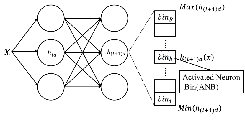
Figure 5: A schematic of k-multisection coverage in a DNN model.

For Experiment 4.4 Coverage Guided Augmention, the set of transformations we consider are : RandomSynonymInsertion, WordSwapEmbedding, WordSwapChangeLocation, WordSwapChangeName, WordSwapChangeNumber, WordSwapContract, WordSwapExtend, WordSwapHomoglyphSwap, WordSwapMaskedLM, WordSwapQWERTY, WordSwapNeighboringCharacterSwap, WordSwapRandomCharacterDeletion, WordSwapRandomCharacterInsertion, WordSwapRandomCharacterSubstitution ,RandomSwap, and WordSwapWordNet.

Test Transformation Name	Failure Rate ($\%$)				Dataset Size Reduction ($\%$)
	D	D+Cover	D+mnCover	$\Delta_{D+\textsc{mnCover}}$	D+Cover	D+mnCover
Change first name in one of the questions	63.00	${\bf 100.00}_{59.40}$	${\bf 100.00}_{64.49}$	${37.00}_{1.49}$	98.20	98.20
add one typo	19.40	${\bf 28.57}_{23.17}$	${\bf 29.41}_{23.52}$	${10.01}_{4.12}$	88.00	88.00
Product of paraphrases(q1) * paraphrases(q2)	95.00	${\bf 100.00}_{100.00}$	${\bf 100.00}_{100.00}$	${5.00}_{5.00}$	99.00	99.00
Replace synonyms in real pairs	8.37	${\bf 13.33}_{7.89}$	${\bf 12.50}_{8.81}$	${4.13}_{0.44}$	73.31	73.31
Symmetry: f(a, b) = f(b, a)	6.00	${\bf 8.33}_{4.83}$	${\bf 10.00}_{4.61}$	${4.00}_{-1.39}$	82.00	82.00
Testing implications	15.07	${\bf 15.25}_{7.90}$	${\bf 15.25}_{7.46}$	${0.19}_{-7.60}$	99.29	99.29
same adjectives, different people v3	100.00	${\bf 100.00}_{100.00}$	${\bf 100.00}_{100.00}$	${0.00}_{0.00}$	81.82	81.82
same adjectives, different people	100.00	${\bf 100.00}_{100.00}$	${\bf 100.00}_{100.00}$	${0.00}_{0.00}$	81.48	81.48
Change same location in both questions	5.00	${0.00}_{0.00}$	${0.00}_{0.00}$	${-5.00}_{-5.00}$	96.60	96.60
Average Improvement	-	$5.96_{-0.96}$	$6.15_{-0.33}$	$6.15_{-0.33}$	$88.86$	$88.86$

Table 6: Failure Rate(%) obtained using BERT model on the original dataset $D$, the dataset filtered using Cover coverage (D+Cover columns) and the dataset filtered with mnCover coverage (D+mnCover columns) from the QQP Suite. We report both the max failure rate as well as the mean in the subscript across $10$ thresholds of coverage. Rows are sorted regarding the failure rate difference between the dataset filtered using mnCover and the original dataset (column $\Delta_{D+\textsc{mnCover}}$). We use $200$ samples in this case.

References

- Belinkov and Bisk (2017) Yonatan Belinkov and Yonatan Bisk. 2017. Synthetic and natural noise both break neural machine translation. arXiv preprint arXiv:1711.02173.
- Belinkov and Glass (2019) Yonatan Belinkov and James Glass. 2019. Analysis methods in neural language processing: A survey. Transactions of the Association for Computational Linguistics, 7:49–72.
- Bommasani et al. (2021) Rishi Bommasani, Drew A Hudson, Ehsan Adeli, Russ Altman, Simran Arora, Sydney von Arx, Michael S Bernstein, Jeannette Bohg, Antoine Bosselut, Emma Brunskill, et al. 2021. On the opportunities and risks of foundation models. arXiv preprint arXiv:2108.07258.
- Devlin et al. (2019) Jacob Devlin, Ming-Wei Chang, Kenton Lee, and Kristina Toutanova. 2019. Bert: Pre-training of deep bidirectional transformers for language understanding.
- Dola et al. (2021) Swaroopa Dola, Matthew B. Dwyer, and Mary Lou Soffa. 2021. Distribution-aware testing of neural networks using generative models. In 43rd IEEE/ACM International Conference on Software Engineering. To appear.
- Jang et al. (2016) Eric Jang, Shixiang Gu, and Ben Poole. 2016. Categorical reparameterization with gumbel-softmax. arXiv preprint arXiv:1611.01144.
- Kiela et al. (2021) Douwe Kiela, Max Bartolo, Yixin Nie, Divyansh Kaushik, Atticus Geiger, Zhengxuan Wu, Bertie Vidgen, Grusha Prasad, Amanpreet Singh, Pratik Ringshia, et al. 2021. Dynabench: Rethinking benchmarking in nlp. arXiv preprint arXiv:2104.14337.
- Kipf and Welling (2016) Thomas N Kipf and Max Welling. 2016. Semi-supervised classification with graph convolutional networks. arXiv preprint arXiv:1609.02907.
- Koh and Liang (2020) Pang Wei Koh and Percy Liang. 2020. Understanding black-box predictions via influence functions.
- Koh et al. (2021) Pang Wei Koh, Shiori Sagawa, Henrik Marklund, Sang Michael Xie, Marvin Zhang, Akshay Balsubramani, Weihua Hu, Michihiro Yasunaga, Richard Lanas Phillips, Irena Gao, et al. 2021. Wilds: A benchmark of in-the-wild distribution shifts. In International Conference on Machine Learning, pages 5637–5664. PMLR.
- Lin and Bilmes (2009) Hui Lin and Jeff Bilmes. 2009. How to select a good training-data subset for transcription: Submodular active selection for sequences. Technical report, WASHINGTON UNIV SEATTLE DEPT OF ELECTRICAL ENGINEERING.
- Lin and Bilmes (2010) Hui Lin and Jeff Bilmes. 2010. An application of the submodular principal partition to training data subset selection. In NIPS workshop on Discrete Optimization in Machine Learning. Citeseer.
- Liu et al. (2019) Yinhan Liu, Myle Ott, Naman Goyal, Jingfei Du, Mandar Joshi, Danqi Chen, Omer Levy, Mike Lewis, Luke Zettlemoyer, and Veselin Stoyanov. 2019. Roberta: A robustly optimized bert pretraining approach. arXiv preprint arXiv:1907.11692.
- Ma et al. (2018a) Lei Ma, Felix Juefei-Xu, Fuyuan Zhang, Jiyuan Sun, Minhui Xue, Bo Li, Chunyang Chen, Ting Su, Li Li, Yang Liu, et al. 2018a. Deepgauge: Multi-granularity testing criteria for deep learning systems. In Proceedings of the 33rd ACM/IEEE International Conference on Automated Software Engineering, pages 120–131.
- Ma et al. (2018b) Lei Ma, Fuyuan Zhang, Minhui Xue, Bo Li, Yang Liu, Jianjun Zhao, and Yadong Wang. 2018b. Combinatorial testing for deep learning systems. arXiv preprint arXiv:1806.07723.
- Morris et al. (2020) John X. Morris, Eli Lifland, Jin Yong Yoo, Jake Grigsby, Di Jin, and Yanjun Qi. 2020. Textattack: A framework for adversarial attacks, data augmentation, and adversarial training in nlp.
- Naik et al. (2018) Aakanksha Naik, Abhilasha Ravichander, Norman Sadeh, Carolyn Rose, and Graham Neubig. 2018. Stress test evaluation for natural language inference. arXiv preprint arXiv:1806.00692.
- Pei et al. (2017) Kexin Pei, Yinzhi Cao, Junfeng Yang, and Suman Jana. 2017. Deepxplore: Automated whitebox testing of deep learning systems. In proceedings of the 26th Symposium on Operating Systems Principles, pages 1–18.
- Prabhakaran et al. (2019) Vinodkumar Prabhakaran, Ben Hutchinson, and Margaret Mitchell. 2019. Perturbation sensitivity analysis to detect unintended model biases. arXiv preprint arXiv:1910.04210.
- Rezende and Mohamed (2015) Danilo Rezende and Shakir Mohamed. 2015. Variational inference with normalizing flows. In International conference on machine learning, pages 1530–1538. PMLR.
- Ribeiro et al. (2019) Marco Tulio Ribeiro, Carlos Guestrin, and Sameer Singh. 2019. Are red roses red? evaluating consistency of question-answering models. In Proceedings of the 57th Annual Meeting of the Association for Computational Linguistics, pages 6174–6184.
- Ribeiro et al. (2018) Marco Tulio Ribeiro, Sameer Singh, and Carlos Guestrin. 2018. Semantically equivalent adversarial rules for debugging nlp models. In Proceedings of the 56th Annual Meeting of the Association for Computational Linguistics (Volume 1: Long Papers), pages 856–865.
- Ribeiro et al. (2020) Marco Tulio Ribeiro, Tongshuang Wu, Carlos Guestrin, and Sameer Singh. 2020. Beyond accuracy: Behavioral testing of nlp models with checklist.
- Tian et al. (2018) Yuchi Tian, Kexin Pei, Suman Jana, and Baishakhi Ray. 2018. Deeptest: Automated testing of deep-neural-network-driven autonomous cars. In Proceedings of the 40th international conference on software engineering, pages 303–314.
- Vaswani et al. (2017) Ashish Vaswani, Noam Shazeer, Niki Parmar, Jakob Uszkoreit, Llion Jones, Aidan N Gomez, Łukasz Kaiser, and Illia Polosukhin. 2017. Attention is all you need. In Advances in neural information processing systems, pages 5998–6008.
- Xie et al. (2019) Qizhe Xie, Zihang Dai, Eduard Hovy, Minh-Thang Luong, and Quoc V Le. 2019. Unsupervised data augmentation for consistency training. arXiv preprint arXiv:1904.12848.