Classification and mapping of low-statured shrubland cover types in post-agricultural landscapes of the US Northeast

Abstract

Novel plant communities reshape landscapes and pose challenges for land cover classification and mapping that can constrain research and stewardship efforts. In the US Northeast, emergence of low-statured woody vegetation, or shrublands, instead of secondary forests in post-agricultural landscapes is well-documented by field studies, but poorly understood from a landscape perspective, which limits the ability to systematically study and manage these lands. To address gaps in classification/mapping of low-statured cover types where they have been historically rare, we developed models to predict shrubland distributions at 30m resolution across New York State (NYS), using a stacked ensemble combining a random forest, gradient boosting machine, and artificial neural network to integrate remote sensing of structural (airborne LIDAR) and optical (satellite imagery) properties of vegetation cover. We first classified a 1m canopy height model (CHM), derived from a patchwork of available LIDAR coverages, to define shrubland presence/absence. Next, these non-contiguous maps were used to train a model ensemble based on temporally-segmented imagery to predict shrubland probability for the entire study landscape (NYS). Approximately 2.5% of the CHM coverage area was classified as shrubland. Models using Landsat predictors trained on the classified CHM were effective at identifying shrubland (test set AUC=0.893, real-world AUC=0.904), in discriminating between shrub/young forest and other cover classes, and produced qualitatively sensible maps, even when extending beyond the original training data. After ground-truthing, we expect these shrubland maps and models will have many research and stewardship applications including wildlife conservation, invasive species mitigation and natural climate solutions. Our results suggest that incorporation of airborne LiDAR, even from a discontinuous patchwork of coverages, can improve land cover classification of historically rare but increasingly prevalent shrubland habitats across broader areas.

¹ Graduate Program in Environmental Science, State University of New York College of Environmental Science and Forestry, Syracuse, NY, USA
² Department of Sustainable Resources Management, State University of New York College of Environmental Science and Forestry, Syracuse, NY, USA

1 Introduction

Human land use has fundamentally altered vegetation-environment relationships and created legacies that include the emergence of novel communities and ecosystem types (Foster, Motzkin, and Slater 1998; Cramer, Hobbs, and Standish 2008). In post-agricultural landscapes of eastern North America, these legacies include loss of plant diversity (Flinn and Vellend 2005) and widespread homogenization of vegetation composition and structure, relative to historical reconstructions (Foster, Motzkin, and Slater 1998; Flinn, Vellend, and Marks 2005). Widespread abandonment of crop, pasture and industrial lands from the late-19th to middle-20th centuries created an expanding land base for invasion and emergence of novel communities (Williams and Jackson 2007; Fridley 2012; Alexander, Diaz, and Levine 2015), with variable outcomes depending on prior land use practices (Stover and Marks 1998; Benjamin, Domon, and Bouchard 2005; Kulmatiski, Beard, and Stark 2006). Entirely novel communities have emerged in old-fields due to colonization by non-native plants, including invasive woody shrubs, which are much more likely to establish and become dominant in post-agricultural (Johnson et al. 2006; Cramer, Hobbs, and Standish 2008; McCay and McCay 2009) and post-industrial sites (Spiering 2019) compared to closed-canopy forests of any successional age. Meanwhile, secondary forests across the US Northeast, including those established in old fields, often lack sufficient advance regeneration to maintain productivity and resilience to changing disturbance regimes (Dey et al. 2019).

Among the outcomes of these changes, the emergence of low-statured vegetation or shrublands as a more common cover type in the US Northeast has been suggested by numerous field studies, but is poorly understood from a landscape perspective. Here the term shrubland reflects a physiognomic definition following King and Schlossberg (2014), which encompasses several types of plant communities found in the US Northeast, including: 1) young, regenerating or otherwise low-statured closed-canopy forests; 2) wetlands dominated by native shrubs (e.g., Alnus spp) or small-statured trees (e.g, Picea marianas in boreal peatlands); 3) uplands dominated by native shrubs (e.g., Cornus racemosa); and most recently, 4) upland shrub/scrub dominated by invasive woody (e.g., Rhamnus and Lonicera spp) and herbaceous (e.g., Solidago spp) perennials. Among the types above, regenerating forests and invasive shrub/scrub communities are of growing interest for research and management purposes, given their anthropogenic origins, their potential novelty in terms of composition and dynamics, and their implications for biodiversity and ecosystem services (Cramer, Hobbs, and Standish 2008; Hobbs, Higgs, and Harris 2009; Perring, Standish, and Hobbs 2013; Dey et al. 2019). Despite their conservation value as wildlife habitat, especially for songbirds, shrublands are widely unpopular cover types in terms of their perceived aesthetic, recreational and economic values (Askins 2001; King and Schlossberg 2014). Although long disregarded, these lands are rapidly gaining attention in today’s urgent push to implement natural climate solutions (Fargione et al. 2018) and identify marginal or underutilized lands for renewable energy generation.

However, current limitations to the classification and mapping of these cover types pose obstacles to advancing both science and stewardship opportunities (Hobbs, Higgs, and Harris 2009). Shrublands are a very challenging cover class to identify from imagery alone, given the breadth of community types included (as noted above) and the high variability in density and canopy cover that exists within and among those community types (King and Schlossberg 2014). In practical terms this means that, when relying solely on imagery, shrublands encompass a full gradient from resembling herbaceous or barren land to resembling closed-canopy conditions (Brown et al. 2020). Furthermore, shrublands are relatively rare in the US Northeast, making them particularly challenging to identify with standard classification methods (Bogner et al. 2018; Haibo He and Garcia 2009). As a result, imagery-based approaches tend to classify shrubland categories with substantially lower accuracy than other land cover classes (Wickham et al. 2021; Brown et al. 2020).

A solution for this problem might be to incorporate additional, non-imagery sources of remote sensing data into land cover classification methodologies. LiDAR data collected through airborne laser scanning can provide essential information for identifying low-statured vegetation such as early-successional forests (Falkowski et al. 2009). In combination with imagery, LiDAR data can enable continuous, broad-scale estimation of canopy heights and other structural traits which may greatly simplify the task of distinguishing between low-statured and taller closed-canopy cover types (Ruiz et al. 2018). Unfortunately, the cost and logistical challenges of airborne LiDAR collection have constrained its availability to smaller extents and with much longer return intervals than provided by satellite imagery. Yet if canopy structural estimates from airborne LiDAR could be used to label a training dataset in order to fit models using satellite imagery, it should be possible to produce models capable of identifying shrubland with greater accuracy than those trained on imagery alone, while being able to map/model a larger and more contiguous spatial extent than models relying on airborne LiDAR data as predictors. Similar methods have been used to automate labeling imagery used to train models for tree and building detection (Zarea and Mohammadzadeh 2016; Huang et al. 2019), but to our knowledge this data fusion approach has not yet been applied for shrubland mapping.

Here we explored this approach to map shrubland across New York State (NYS), a largely post-agricultural landscape containing extensive old-fields populated mostly by secondary forests or invasive shrub/scrub communities, which are difficult to parse based on imagery alone. We leveraged a non-contiguous patchwork of existing large-footprint LIDAR data sets by creating very high resolution (1 m) canopy height models that covered approximately 60% of the study area (NYS). By sampling from these canopy height maps, we trained machine learning models with temporally segmented Landsat imagery and land cover data products, and created a stacked ensemble to map the probability of shrubland at a high resolution (30 m) across the study area. Models were evaluated across multiple sensitivity/specificity thresholds to generate a range of map outputs that can support future ground-truthing efforts as part of research and stewardship activities. We provide new maps of marginal cover types, such as invasive shrublands and degraded young forests, and demonstrate how to leverage an information-rich but geographically incomplete data source (LIDAR) for large-scale contiguous land cover classification and mapping based on widely available and standardized time-series imagery. Our results suggest that using LiDAR, where it exists, to label data for model training may help distinguish shrublands from other, optically similar land cover classes. We additionally demonstrate the utility of using targeted, regional land cover products to supplement national products for classes of regional interest.

2 Methods

In order to map potential shrubland across New York State, we first identified low-stature vegetation across a discontinuous temporal patchwork of 1m resolution canopy height models (CHMs) derived from 19 distinct LiDAR acquisitions. We then aggregated these 1m identifications into a 30m resolution raster surface, associated this surface with multiple data products derived from temporally matching remote sensing observations (including Landsat imagery as well as climate and topographic data), and used this data to produce a stacked ensemble model composed of a random forest, gradient boosting machine, and artificial neural network combined through a logistic regression. We used this ensemble model to predict shrubland for a spatiotemporal patchwork matching LiDAR acquisitions, as well as for the entire state in 2019. A flowchart of this process is included as Figure 1.

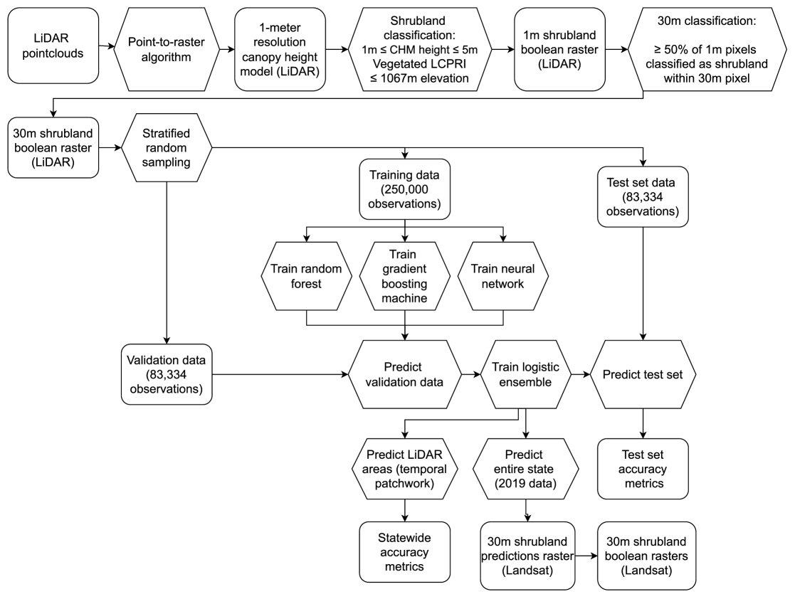
Figure 1: A flowchart diagram showing the key elements of the identification methodology. Rectangular boxes represent data products and results, while hexagonal boxes represent methodological steps.

2.1 Study area

New York State spans an area of 141,297 $\operatorname{km}^{2}$ of the northeastern United States. Extensive land clearing for agriculture and industry in the 18th through 19th centuries decimated forests throughout the region, with forest cover dropping to 10-30% of the landscape by 1880 (Lorimer 2001). While total forest cover recovered rapidly at the turn of the 20th century, these forests were almost entirely young due to the combination of regeneration on abandoned farmland with the continual coppicing and harvesting of more established woodlots for fuelwood and other products (Whitney 1994). A variety of factors, among them a decrease in the use of wood for residential heating and an increase in forest conservation efforts, caused these forests to begin to mature in the 1930s, with the effect that the majority of forest stands across the Northeast are now over 100 years old. Two forest preserves, the Adirondack Park in the northeast and the Catskill Park in the southeast, have been protected in the New York State constitution as “forever wild”; timber harvesting has been generally prohibited on state-owned parcels in these regions since they were incorporated into the Forest Preserve, a process beginning in 1885. As a result, there is very little shrubland in these preserves.

Elevations across New York State range from -2 m to 1,584 m above sea level (U.S. Geological Survey 2019), with daily temperatures in 2019 ranging from -17 °C to 28 °C and monthly precipitation for the same period ranging from 5.0 cm to 16.8 cm (NOAA National Centers for Environmental Information 2022). The majority of the state occupies the northern hardwoods-hemlock forest region, though there are important inclusions of beech-maple-basswood and Appalachian oak communities in the western and southern reaches of the state, respectively (Dyer 2006).

2.2 LiDAR Data and Shrubland Identification

Although a distinction exists between early-successional and young forest habitats in eastern North America, for simplicity we have followed King and Schlossberg (2014) in combining these categories into a single shrubland classification due to their structural similarity. This terminology aligns with Anderson (1976), who described shrubland in the eastern United States as “former croplands or pasture lands (cleared from original forest land) which now have grown up in brush in transition back to forest land to the extent that they are no longer identifiable as cropland or pasture from remote sensor imagery.”

Shrubland was identified using 19 distinct leaf-off LiDAR acquisitions, collected and made freely available as part of the US Geological Survey’s 3D Elevation program. All LiDAR used in this study was collected between 2014 and 2020, with point densities ranging from 1.98 to 3.24 points per square meter (Figure 2). All LiDAR data had a vertical accuracy RMSE of $\leq$ 10 cm. While horizontal accuracy was not typically reported in provided LiDAR metadata, horizontal RMSE for all data sets is expected to be $\leq$ 68 cm (ASPRS 2014). More information about individual LiDAR coverages is available as Supplementary Materials 1. These point clouds were converted to 1 m canopy height models (CHMs) using a point-to-raster algorithm implemented in the lidR R package (Roussel et al. 2020). To reflect the 2D nature of a LiDAR return footprint, and mitigate potential voids in the resulting CHM, each return was replaced with a circle of returns with a diameter equal to the pulse width present in the metadata (default 0.5 m; Supplementary Materials 1). These CHMs were then masked to exclude any pixel assigned a non-vegetation primary land cover classification by the temporally-matching USGS LCMAP land cover product (namely the developed, water, ice and snow, and barren classes) using the terra R package (Brown et al. 2020; Hijmans 2021; R Core Team 2021). CHMs were also masked to exclude any pixel with an elevation above 1067m (3500 ft), as shorter canopy heights at these elevations likely represent krumhholz (stunted trees near elevational treeline) instead of shrubs or regenerating forest. Shrubland was then defined as any 1 m pixel with a CHM height between 1-5 m. The lower threshold was defined to avoid classifying cropland and human structures (such as low walls) as shrubland, and the upper threshold defined to match the USGS NLCD definition of shrubland, which was derived from the Anderson classification system (Yang et al. 2018; Anderson et al. 1976). While this coarse definition allows for efficient and automated labeling of data, it also has its limitations, including being reliant upon the accuracy and unbiasedness of LCMAP class predictions and potentially incorrectly classifying some cropland, including orchards, as shrublands. To evaluate these limitations, we validated model predictions using manual inspection of optical imagery, described further in Section 2.4.

These 1 m pixels were then aggregated into 30 m resolution pixels using GDAL (GDAL/OGR contributors 2021), with each 30 m pixel defined as shrubland if more than 50% of its constituent 1 m subpixels were identified as shrubland.

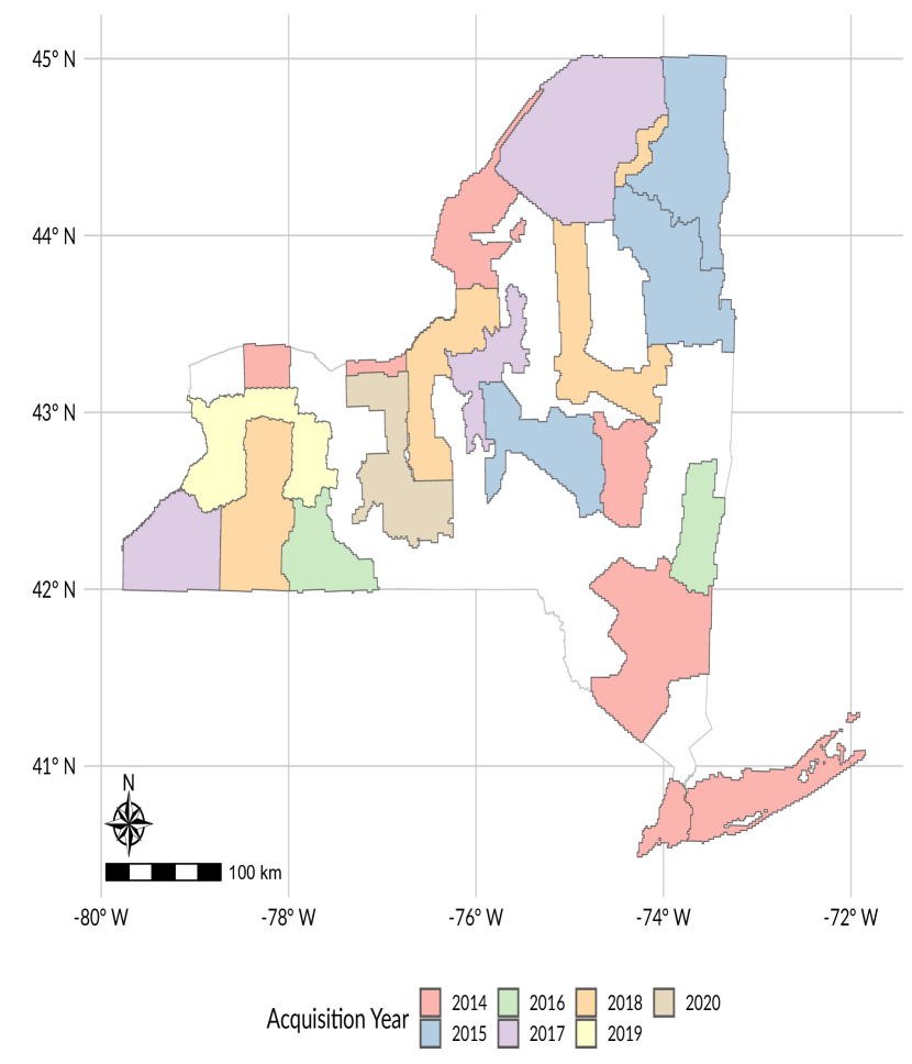
Figure 2: Boundaries for all LiDAR coverages used in this project, colored by year of data acquisition. More information about each coverage is included as Online Resource 1.

2.3 Predictor Creation

We produced a set of 10 annual Landsat-derived predictors by processing Landsat analysis ready data (ARD, Dwyer et al. 2018) in Google Earth Engine (GEE, Gorelick et al. 2017), using a medoid composite of imagery acquired between July 1st and September 1st of the same year LiDAR was acquired at each pixel. Landsat ARD was processed using the LandTrendr implementation in GEE (hereafter LT-GEE) to fill gaps (e.g., clouds and shadows) in the annual time series, smooth interannual variations (noise), and quantify the disturbance history for each pixel (Kennedy, Yang, and Cohen 2010; Kennedy et al. 2018). The LT-GEE predictors included three tasseled cap indices, (brightness - TCB, greenness - TCG, and wetness - TCW) and their respective deltas computed with a 1-year lag, all fit to Normalized Burn Ratio (NBR) temporally segmented vertices, as well as an NBR index and respective 1-year delta (Kauth and Thomas 1976; Cocke, Fulé, and Crouse 2005; Kennedy et al. 2018). We also processed a separate NBR segmented time-series with LT-GEE parameters tailored to be more sensitive to the timing of discrete disturbances using LT-GEE code to produce two predictors describing disturbances at an individual pixel: year-of-most-recent-disturbance (YOD; 1985-2020) and associated magnitude-of-most-recent-disturbance (MAG; unitless measure of change in NBR value) (Kennedy et al. 2018). All predictors are described in Table 1. The 8 annual indices and associated deltas aimed to capture the surface reflectance for a given pixel at a given time, while the two disturbance predictors aimed to describe disturbance history for a given pixel. NBR was chosen as the base predictor, providing disturbance history information and temporal break-points to which tasseled cap predictors were fit, as it has been shown to be the most sensitive for capturing disturbance events (Kennedy, Yang, and Cohen 2010). Information on LT-GEE parameters used is included as Supplementary Materials 2.

Table 1: Definitions of predictors used for model fitting.

Predictor	Definition
TCB, TCW, TCG	Tassled cap brightness, wetness, and greenness, with noise removed using LT-GEE
NBR	Normalized burn ratio with noise removed using LT-GEE
MAG, YOD	Magnitude and year of most recent disturbance, as identified using LT-GEE
PRECIP, TMAX, TMIN	30-year normals for precipitation, maximum temperaure, and minimum temperature, derived from annual PRISM climate models
ASPECT, ELEVATION, SLOPE, TWI	Aspect, elevation, slope, and topographic wetness index derived from a 30-meter digital elevation model
LCSEC	LCMAP secondary land cover classification

In addition to Landsat-derived predictors, a set of steady-state ancillary predictors was included to represent geospatial variation in climate and topography (Kennedy et al. 2018). These predictors included precipitation and temperature 30 year normals derived from PRISM Climate Group data (PRISM Climate Group 2022), the secondary land cover classification prediction from LCMAP (Brown et al. 2020), and elevation, aspect, slope, and topographic wetness indices derived from a 30 meter digital elevation model (Mahoney, Beier, and Ackerman 2022; U.S. Geological Survey 2019; Beven and Kirkby 1979). In total, models were fit using 14 separate predictors (Table 1).

2.4 Model Fitting and Evaluation

Each LiDAR-derived shrubland layer was combined with a set of temporally matching predictors, which were then merged into a single temporal patchwork data set representing each region of the state during its year of LiDAR acquisition. A total of 416,668 pixels were then sampled from this patchwork set (Figure 1), stratified so that half (208,334) represented shrubland and half other land cover types. These pixels were then split at random into a training set of 250,000 pixels, a validation set of 83,334 pixels, and a hold-out evaluation set of 83,334 pixels. We then fit three separate models, a random forest (Breiman 2001), stochastic gradient boosting machine (Friedman 2002), and deep neural network (LeCun, Bengio, and Hinton 2015), against the training data set to estimate the probability of a given pixel representing shrubland. Models were fit using hyperparameters chosen to minimize out-of-sample binary cross entropy (Good 1952).

The random forest was fit using 3,000 trees, each using a random bootstrap sample of 20% of the data, sampled with replacement, a minimum node size of 6 observations, a single random variable per split, and splitting to minimize Gini impurity. The gradient boosting machine was fit using 2,500 trees, each with unlimited depth, a maximum of 14 leaves, a learning rate of 0.01, a minimum of 10 observations per leaf and 3 observations per bin, an L1 regularization constant of 0 and a L2 regularization constant of 0.5. Each tree was fit using a new bootstrap sample with half the number of observations as the training data, with access to 90% of predictors. The neural net was a simple additive neural network with seven layers: five densely connected layers with numbers of nodes halving with each additional layer, decreasing from 256 to 128 to 64 to 32 to 16, then feeding into a 20% dropout layer before the final densely connected output layer with a single node. All dense layers used rectified linear activation functions save for the output layer, which used a sigmoid activation function. The model was trained using 1,000 epochs, but final weights used the epoch which maximized the area under the precision-recall curve of the validation data set.

We then used each of these models to predict the probability of a pixel representing shrubland for each observation in the validation data set. Next, we fit a logistic regression to the validation set predictors and predicted probabilities to combine our three models into a single stacked ensemble model (Wolpert 1992; Dormann et al. 2018). This ensemble model was then used to generate predictions for the test set, for the temporal patchwork data set, and for data reflecting the entire state for 2019 (chosen in order to compare predictions to the 2019 NLCD land cover map). The same model was used for predicting each of these data sets.

Probability thresholds used to classify individual pixels were chosen using model predictions for the validation set. Four separate thresholds were identified: the one that maximized the model’s summed sensitivity (Equation 1) and specificity (Equation 2), calculated using Youden’s J statistic (hereafter ‘Youden Optimal’) (Youden 1950); and three that maximized sensitivity while keeping specificity above 90%, 95%, and 99%. All accuracy metrics were assessed using the temporal patchwork data set, with Landsat-derived predictors temporally matched to the LiDAR data set. All metrics were calculated considering shrubland pixels as positive cases; higher specificity targets reflected the relatively rare abundance of shrubland throughout the state (approximately 2.5% of mapped pixels) necessitating low levels of false positives. Predictions against both the test set and the temporal patchwork data set were classified using each of these thresholds, then assessed using sensitivity (Equation 1), specificity (Equation 2), precision (Equation 3), and F1 score (Equation 4).

$$\hypertarget{eq-sens}{}{\operatorname{Sensitivity}=\frac{T_{\operatorname{Positives}}}{T_{\operatorname{Positives}}+F_{\operatorname{Negatives}}}}$$ (1)

$$\hypertarget{eq-spec}{}{\operatorname{Specificity}=\frac{T_{\operatorname{Negatives}}}{F_{\operatorname{Positives}}+T_{\operatorname{Negatives}}}}$$ (2)

$$\hypertarget{eq-prec}{}{\operatorname{Precision}=\frac{T_{\operatorname{Positives}}}{T_{\operatorname{Positives}}+F_{\operatorname{Positives}}}}$$ (3)

$$\hypertarget{eq-f1}{}{\operatorname{F1}=\frac{2*\operatorname{Precision}*\operatorname{Sensitivity}}{\operatorname{Precision}+\operatorname{Sensitivity}}}$$ (4)

Where $T_{\operatorname{Positives}}$ is the number of pixels correctly classified as shrubland, $F_{\operatorname{Positives}}$ the number of pixels incorrectly classified as shrubland, $T_{\operatorname{Negatives}}$ the number of pixels correctly classified as not being shrubland, and $F_{\operatorname{Negatives}}$ the number of pixels incorrectly classified as not being shrubland.

Models were additionally assessed using the area under the receiver operating characteristic curve (AUC) (Austin and Steyerberg 2012), calculated for the test set using all observations and for the temporal patchwork set using a random sample of 1,000,000 pixels due to computational limitations. Given the imbalance of our classes, we do not report overall accuracy or balanced accuracy for either the test set or the temporal patchwork, given that approximately 97.5% overall accuracy could be achieved by never predicting shrubland.

A final assessment involved comparing a stratified sample of model predictions to 1m resolution 2019 imagery from the National Agricultural Inventory Program (US Department of Agriculture 2019). Predictions from the 2019 ensemble model were stratified spatially into 51 16,974 $\operatorname{km}^{2}$ hexagons (equaling an apothem of 70 kilometers). Within each hexagon, five pixels were randomly selected from each of 12 probability bins (predicted probabilities from the ensemble model between 0% and 5%, 5% and 10%, 90% and 95%, and 95% and 100%, as well as each decile between 10% and 90%). Samples taken for two additional bins, ranging from 0% to 1% and 99% to 100%, were merged into the 0% to 5% and 95% to 100% bins due to the rarity of these extreme probabilities, resulting in these bins having slightly more observations. When regions of a hexagon extended beyond the mapped area, the number of pixels selected per bin was scaled in proportion to the mapped region of the hexagon. Pixels were classified as either clearly representing shrubland, clearly representing a non-shrubland class, or as “unknown” if the correct classification could not be ascertained from imagery. A single rater classified all validation pixels.

All models were fit using either R version 4.1.2 (R Core Team 2021) or Python version 3.9.10 (Python Core Team 2022). Random forests were fit using the ranger R package (Wright and Ziegler 2017), gradient boosting machines using lightgbm (Ke et al. 2017), and neural nets using keras (Chollet 2015).

3 Results

3.1 LiDAR Classification

Based on LIDAR-derived CHMs, approximately 2.5% of the study area was initially mapped as shrubland (1-5 m tall), representing about $1.83x10^{6}$ ha of the $73.3x10^{6}$ ha land area that remained after LCMAP masking removed non-vegetated cover types (Figure 3). Shrubland was identified in every LiDAR coverage, with proportions ranging from 0.3% (Great Gully) to 7.6% (Great Lakes) of the coverage footprint area (Figure 3).

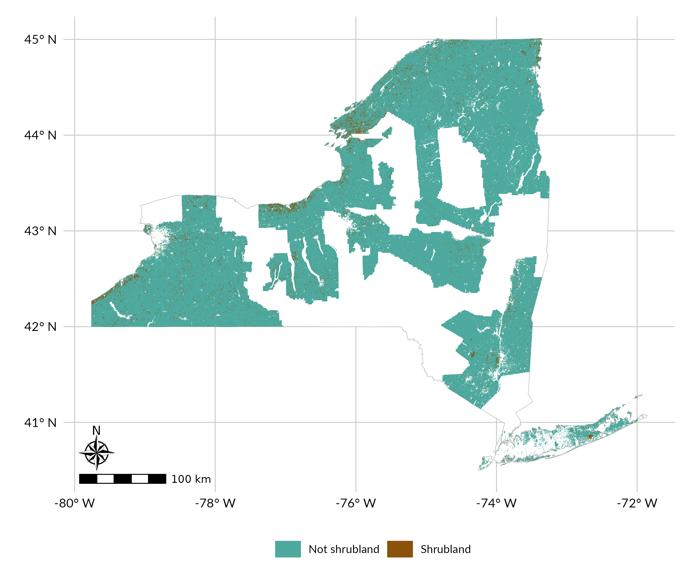
Figure 3: Identified shrubland areas within each available LiDAR coverage. Shrubland was defined at a 1 meter resolution as being any area within a vegetated LCPRI land cover class and below 1067 meters elevation with a LiDAR-derived height between 1 and 5 meters. 30 meter pixels, used for analysis and modeling, were then defined as shrubland if more than 50% of their contained 1 meter pixels were classified as shrubland. In total, approximately 2.5% of 30 meter pixels were classified as shrubland.

Shrubland cover was present in each vegetated LCMAP primary classification classes, but was weighted more heavily towards areas classified as cropland or tree cover (Table 2). Approximately 7.3% of land classified by LCMAP as “grassland/shrub” was classified as shrubland through this process, though this result should not be over-interpreted given the LCMAP “grassland/shrub” category includes herbaceous land covers alongside shrublands (Brown et al. 2020).

Table 2: Total area and amount of shrubland within each LCMAP primary land cover classification (“LCPRI”), in square kilometers, for each map surface (bolded text). Both the temporal patchwork and statewide models were classified using a 95% specificity threshold.

LCPRI	Total area	Shrubland area	% Shrubland
LiDAR Classification
Cropland	20 077.6	679.5	3.4%
Grass/Shrub	2 085.3	151.8	7.3%
Tree Cover	44 879.5	597.2	1.3%
Wetland	6 635.0	467.9	7.1%
Temporal Patchwork
Cropland	20 077.6	1 451.2	7.2%
Grass/Shrub	2 085.3	416.2	20.0%
Tree Cover	44 879.5	1 428.3	3.2%
Wetland	6 635.0	1 166.3	17.6%
2019 Statewide
Cropland	29 922.9	2 005.9	6.7%
Grass/Shrub	2 994.2	549.3	18.3%
Tree Cover	69 419.0	1 694.6	2.4%
Wetland	9 008.3	1 425.0	15.8%

3.2 Model Accuracy

The ensemble model had a higher AUC than the individual component models on both the test set (Ensemble 0.893; random forest 0.843; gradient boosting machine 0.889; neural network 0.883) and a random sample of $1x10^{6}$ pixels from the LiDAR temporal patchwork data set (Ensemble 0.904; random forest 0.844; gradient boosting machine 0.890; neural network 0.901) (Figure 4; Supplementary Materials 3). As a result, we focus here on accuracy assessments for the ensemble model; accuracy assessments for the component models are included as Supplementary Materials 3.

When evaluating models against the balanced test set, the highest F1 score (0.816) was achieved using the Youden-optimal classification threshold (Table 3). The model retained its high AUC, sensitivity, and specificity when predicting the LiDAR temporal patchwork data set, precision was lower due to the large imbalance between shrubland and other cover classes across the state. As a result, the model attained its highest F1 score of 0.307 when using a classification threshold to that targeted 95% specificity.

Table 3: Model accuracy metrics for logistic ensemble model with predictions classified using various thresholds, calculated using both the balanced test set and the LiDAR patchwork surface. AUC for the LiDAR patchwork was calculated using a random sample of 1,000,000 pixels, while all other metrics used all predicted pixels. Thresholds were selected using a separate validation set, using values chosen to maximize the Youden J statistic (‘Youden optimal’) or to target a certain minimum specificity (‘% specificity’).

	Threshold	Sensitivity	Specificity	Precision	F1
Test set (AUC: 0.893)
Youden optimal	0.489	0.842	0.780	0.791	0.816
90% specificity	0.755	0.659	0.900	0.867	0.807
95% specificity	0.840	0.496	0.949	0.906	0.641
99% specificity	0.907	0.218	0.989	0.952	0.355
LiDAR patchwork (AUC: 0.904)
Youden optimal	0.489	0.858	0.783	0.094	0.169
90% specificity	0.755	0.689	0.896	0.149	0.245
95% specificity	0.840	0.514	0.951	0.219	0.307
99% specificity	0.907	0.247	0.989	0.376	0.298

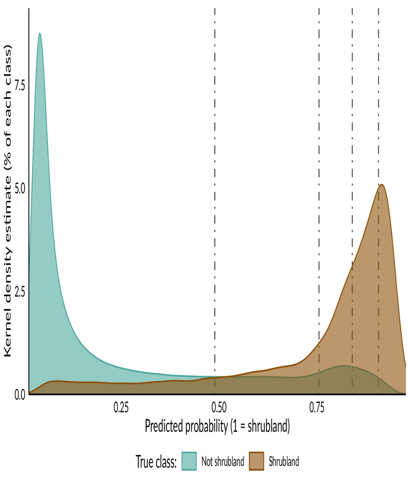
Figure 4: Smoothed kernel density estimates of predicted probability of shrubland for both shrubland and non-shrubland pixels, calculated using a random sample of 1,000,000 pixels taken from the LiDAR patchwork prediction surface using the logistic ensemble model. Vertical lines indicate each of the four probability thresholds used to classify pixels. Colors represent the correct classification of the pixel.

3.2.1 LiDAR Patchwork Predictions

When predicting the temporal patchwork, our model predicted the highest probabilities of shrubland along the northern reaches of the state, matching the distribution of shrubland in the true LiDAR-derived surface (Figure 5). However, the model also predicted higher than average probabilities of shrubland in the southwestern and central regions of the state, neither of which were reflected in the original LiDAR-derived surface.

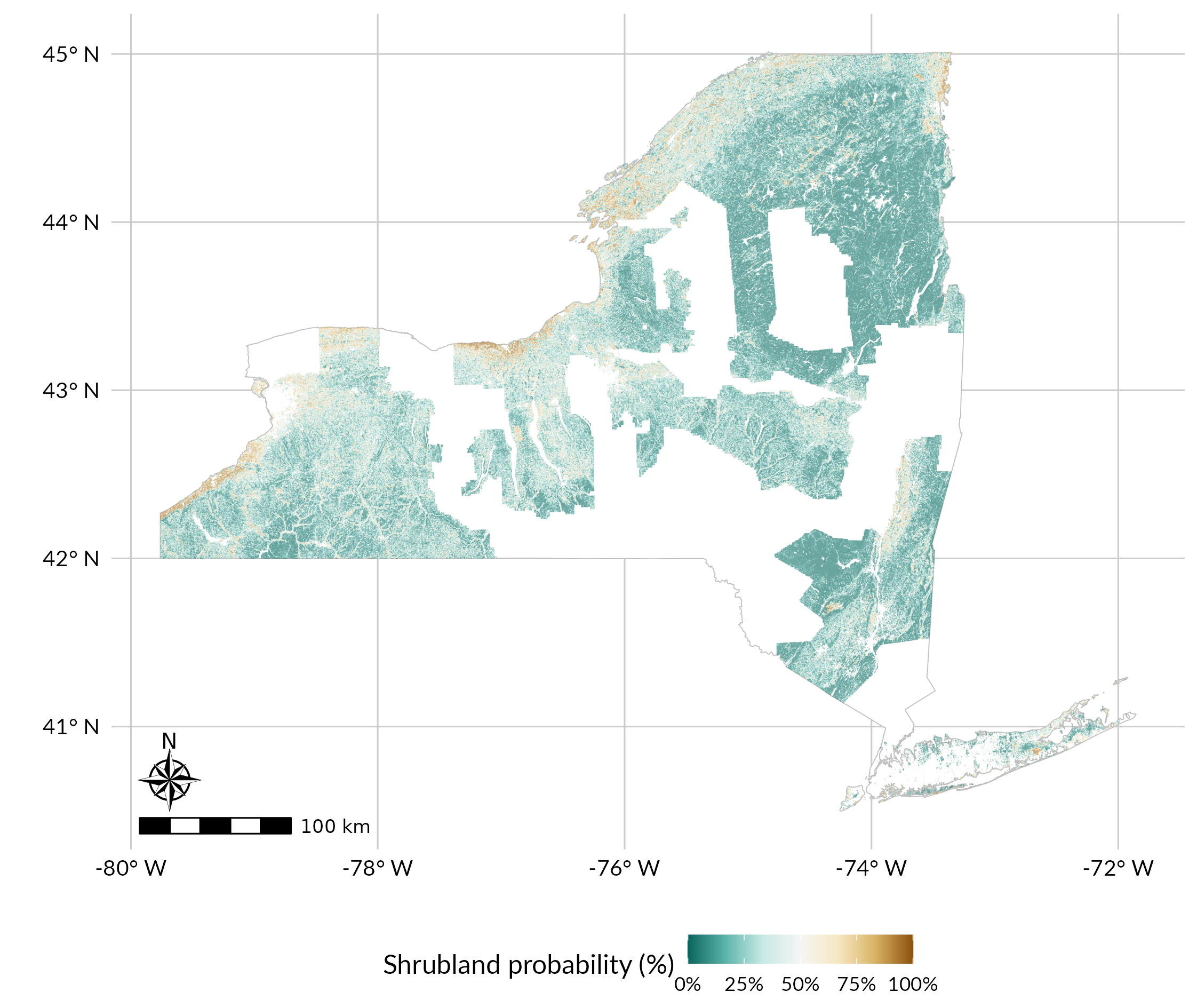
Figure 5: Predicted probability of shrubland for the boundaries of all used LiDAR coverages, from the logistic ensemble model. Predictions were made using data reflecting the same year as LiDAR acquisition; the map therefore represents a temporal patchwork of predictions. Pixels in non-vegetated LCPRI land cover classes (developed, water, ice/snow, and barren) or above 1067 meters in elevation were not mapped and are shown in white.

Boolean surfaces classified using the Youden optimal probability threshold classified 23% of pixels as shrubland, an order of magnitude greater than the 2.5% identified from the true LiDAR-derived surface (Figure 6). More conservative predictions based on specificity thresholds predicted a lower proportion of shrubland (90% specificity: 11.9%; 95% specificity: 6.1%, 99% specificity: 1.7%) with a higher precision, resulting in more accurate overall predictions and higher F1 scores.

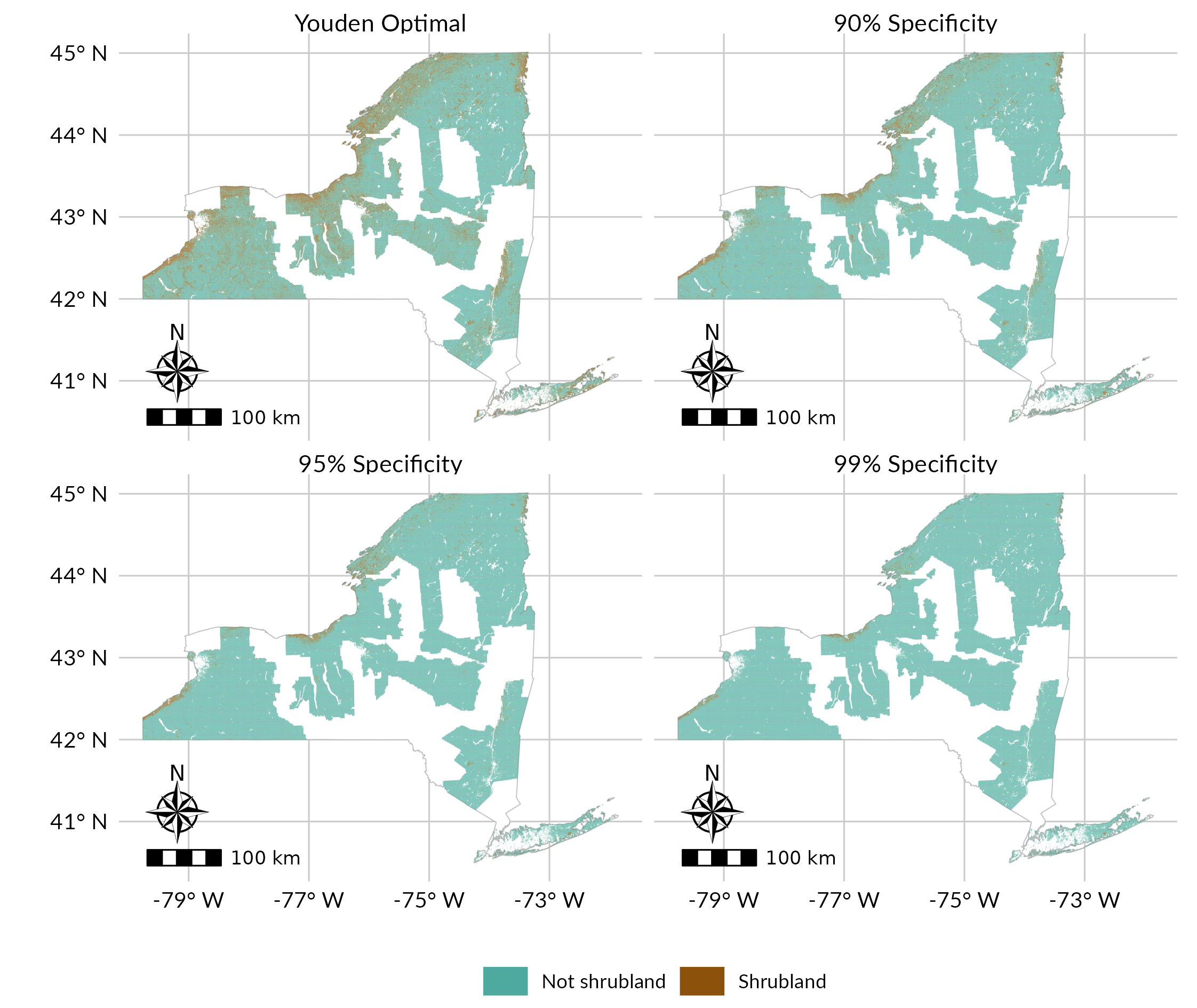
Figure 6: Predicted shrubland locations within each LiDAR coverage, from the logistic ensemble model. Predicted pixel probabilities were classified using either the Youden-optimal threshold (which maximizes both sensitivity and specificity) or a threshold chosen to target a certain level of specificity, using thresholds derived from the validation data set. Predictions were made using data reflecting the same year as LiDAR acquisition; the map therefore represents a temporal patchwork of predictions. Pixels in non-vegetated LCPRI land cover classes (developed, water, ice/snow, and barren) or above 1067 meters in elevation were not mapped and are shown in white.

3.2.2 2019 Statewide Predictions

Model predictions reflected a similar geographical distribution of shrubland when extrapolating beyond the spatiotemporal boundaries of available LiDAR data to map shrubland across the entire state for 2019. Areas throughout the Adirondack Park and the Catskill Park, montane regions with mostly contiguous forest cover, showed notably less shrubland than more heavily populated areas (Figure 7). As expected, predictions in areas included in the LiDAR patchwork data set resembled the predictions for the LiDAR patchwork surface (Figure 5), though with some variation due in part to the temporal mismatch.

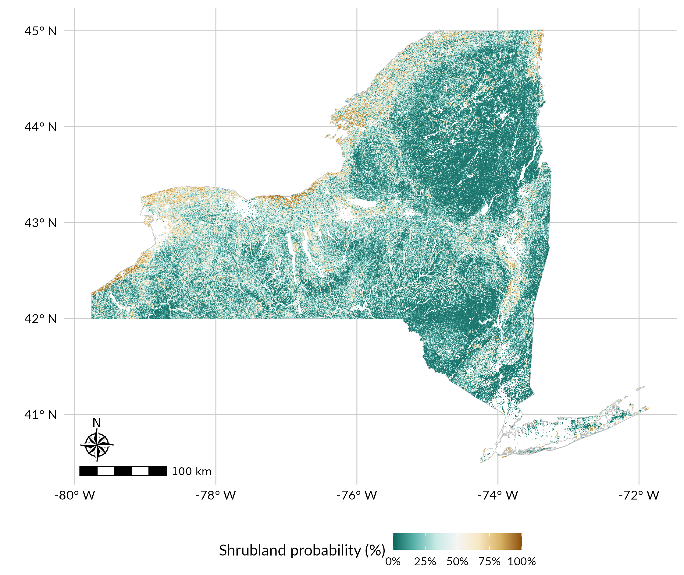
Figure 7: Predicted probability of shrubland for 2019 across all mapped areas within New York State, from the logistic ensemble model. Pixels in non-vegetated LCPRI land cover classes (developed, water, ice/snow, and barren) or above 1067 meters in elevation were not mapped and are shown in white.

Shrubland probabilities were highest in areas classified by 2019 LCMAP as shrubland, as well as in areas classified as wetlands by either LCMAP or NLCD (Figure 8). Areas classified as tree cover were assigned extremely low probabilities.

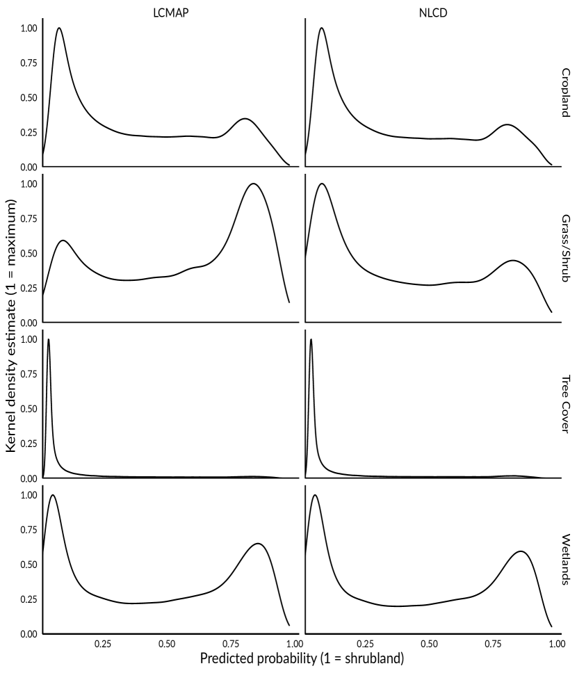
Figure 8: Smoothed kernel density estimates of predicted probability of shrubland for the included LCMAP classes, calculated using a random sample of 1,000,000 pixels taken from the LiDAR patchwork prediction surface using the logistic ensemble model. Density estimates have been rescaled so that the most common probability for each panel is assigned a value of 1. NLCD land cover classes were remapped to LCMAP classes using LCMAP-defined translations.

Predictions for 2019 classified using the Youden optimal probability threshold classified 22.3% of the state as shrubland (Figure 9), in line with the Youden optimal classified LiDAR patchwork data set. The target-specificity thresholds classified more realistic proportions (90% specificity: 10.7%; 95% specificity: 5.1%, 99% specificity: 1.2%).

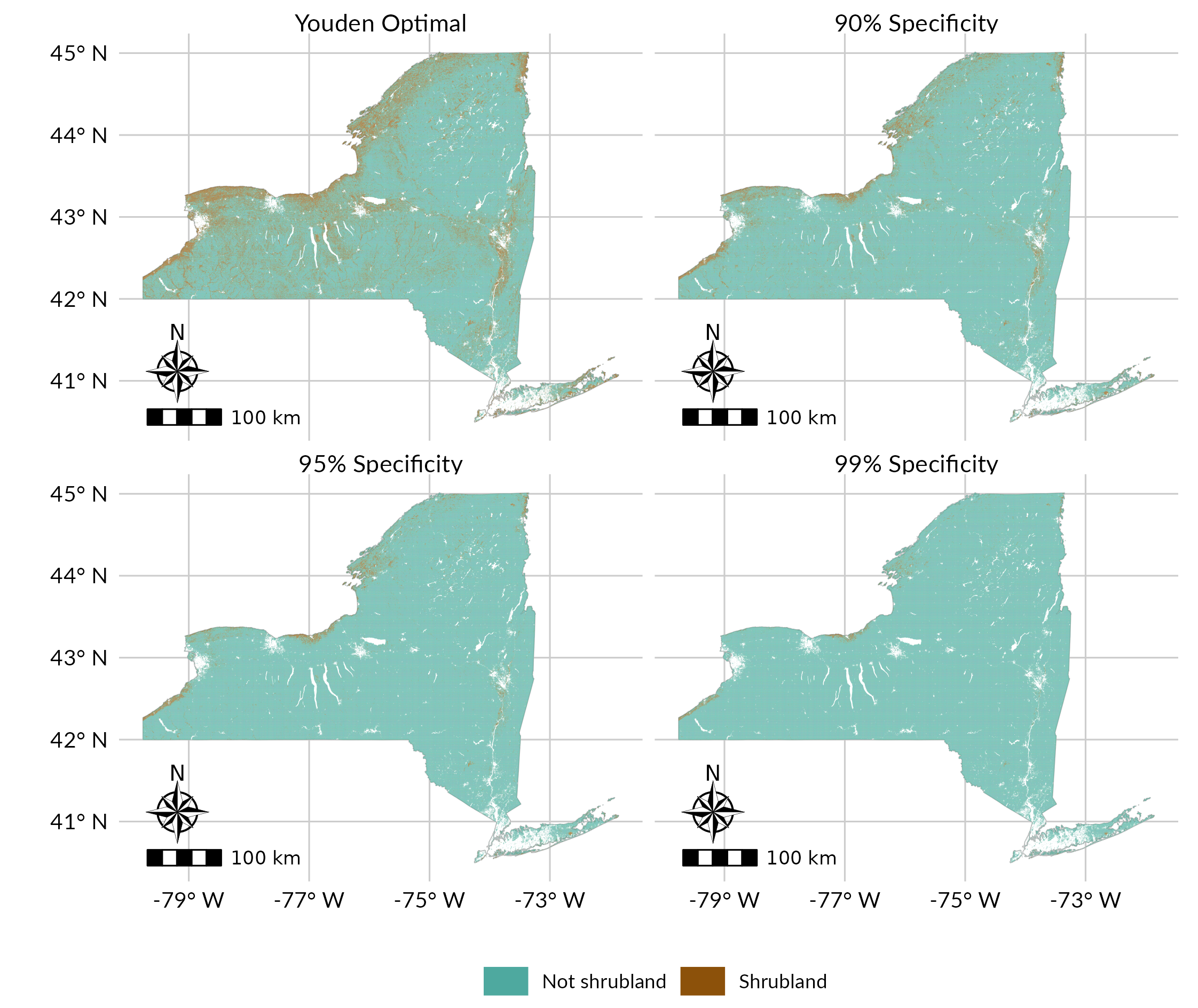
Figure 9: Predicted shrubland locations for 2019 across the entire state, from the logistic ensemble model. Predicted pixel probabilities were classified using either the Youden-optimal threshold (which maximizes both sensitivity and specificity) or a threshold chosen to target a certain level of specificity, using thresholds derived from the validation data set. Pixels in non-vegetated LCPRI land cover classes (developed, water, ice/snow, and barren) or above 1067 meters in elevation were not mapped and are shown in white.

3.2.3 Validation Using 2019 Imagery

Pixels with a higher predicted probability of shrubland were generally more likely to represent shrubland, as determined using predictions and imagery from 2019 (Table 4). Pixels with a nominal predicted probability of shrubland at or above 0.95 were less likely to actually represent shrubland than pixels with probabilities between 0.8 and 0.95, suggesting a failure to generalize to pixels with predictor values outside the ranges reflected in the training data (Efron 2020) (Table 4).

Table 4: True classification of map pixels at various predicted shrubland probabilities. Numbers in parentheses reflect the percentage of pixels in each probability bracket in a given classification. Samples taken for two additional bins, ranging from 0% to 1% and 99% to 100%, were merged into the 0% to 5% and 95% to 100% bins due to the rarity of these extreme probabilities, resulting in these bins having slightly more observations.

		True classification (from imagery)
Predicted probability of shrubland	# in sample	Not shrubland	Unknown	Shrubland
(0,0.05]	163	158 (96.9%)	5 (3.1%)	0 (0.0%)
(0.05,0.1]	159	144 (90.6%)	11 (6.9%)	4 (2.5%)
(0.1,0.2]	159	137 (86.2%)	18 (11.3%)	4 (2.5%)
(0.2,0.3]	159	130 (81.8%)	17 (10.7%)	12 (7.5%)
(0.3,0.4]	159	121 (76%)	19 (12%)	19 (12%)
(0.4,0.5]	159	118 (74.2%)	24 (15.1%)	17 (10.7%)
(0.5,0.6]	158	114 (72.2%)	26 (16.5%)	18 (11.4%)
(0.6,0.7]	159	104 (65.4%)	25 (15.7%)	30 (18.9%)
(0.7,0.8]	159	100 (62.9%)	24 (15.1%)	35 (22.0%)
(0.8,0.9]	159	70 (44.0%)	25 (15.7%)	64 (40.3%)
(0.9,0.95]	159	48 (30%)	30 (19%)	81 (51%)
(0.95,1]	240	154 (64%)	16 (7%)	70 (29%)

The majority of shrubland pixels, as identified using imagery, were classified as either tree cover or wetland pixels in both NLCD and LCMAP (Figure 10). The majority of non-shrubland pixels with a high predicted probability of shrubland were classified as cropland by LCMAP (Figure 10).

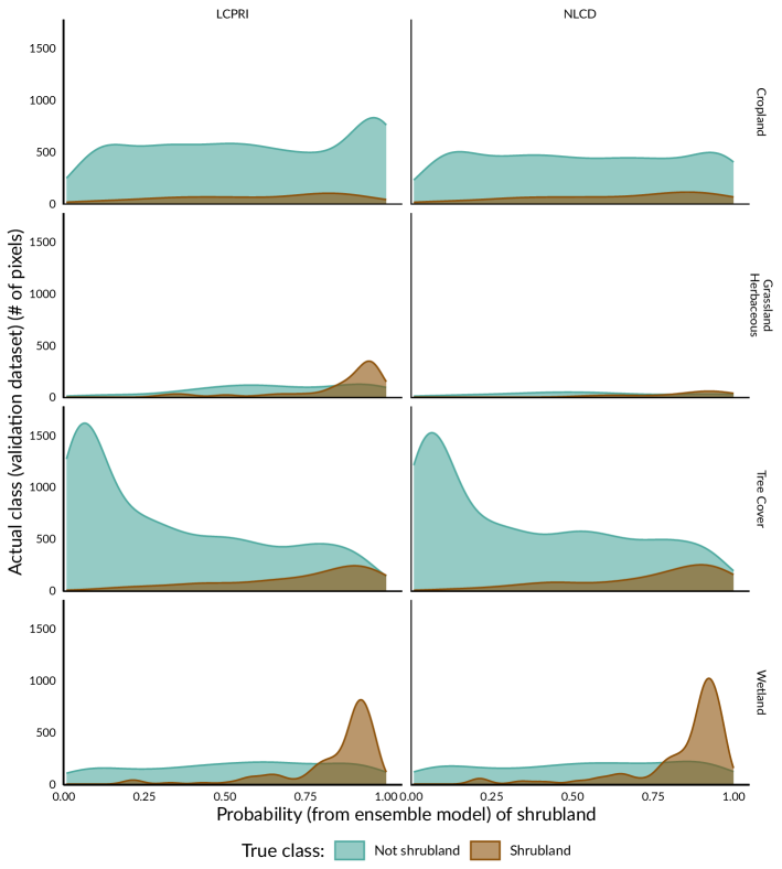
Figure 10: Number of pixels (kernel density estimate) representing shrubland (determined from NAIP imagery) by LCMAP and NLCD classification. Pixels which could not be definitively identified as shrubland are classed as “not shrubland”.

4 Discussion

In this study, we produced a model capable of predicting shrubland locations, as delineated using airborne LiDAR data and LCMAP land cover classifications, across a large, fragmented and heterogenous landscape (New York State). Overall, we found that our models were effective at distinguishing between shrubland and other land cover classes, and produced qualitatively sensible map outputs, even when extrapolating beyond the original training data. Our results serve to demonstrate that incorporating airborne LiDAR data can improve land cover classifications, particularly for marginal, transitional and emergent cover types that may not be well represented in land cover class definitions. More practically, we provide new maps of marginal cover types, such as invasive shrub/scrub and degraded young forests, that have emerged mostly on post-agricultural and post-industrial lands during the last century. While our model has limitations in the labeling of training data and the inherent difficulty in predicting rare events, it was effective at distinguishing between shrubland and other cover types. This modeling approach addresses a persistent measurement gap and enables monitoring, research, and stewardship of these emerging and novel communities at a landscape scale.

4.1 Model predictions reflect known patterns

Our model predictions, both for areas included in the LiDAR patchwork and for the 2019 surface, reflect known patterns in land cover throughout New York State. Although areas classified as developed by LCMAP were excluded from predictions, areas of higher-intensity human land use – such as the Hudson Valley in the eastern region of the state, the I-90 highway corridor running East-West (along roughly 43N latitude), and the northern border of the state, particularly around the Great Lakes – were consistently classified as having a higher probability of shrubland (Figure 5, Figure 7). These areas have likely been more recently impacted by human activity, with cropland only more recently being left to natural regeneration. By the same pattern, areas of lower population density and less intensive land use history such as the Adirondack and Catskill Parks have consistently low probabilities of shrubland, reflecting the older, mid-successional forests that characterize these areas. When extrapolating beyond the spatiotemporal boundaries of available LiDAR data, our 2019 statewide model predicted a similar abundance of shrubland with a similar regional distribution as the LiDAR patchwork data set, with similar areas of shrubland along the Great Lakes and adjacent to human population centers. This pattern reflects the continuing decline in agricultural land across New York State (USDA National Agricultural Statistics Service 2019); while much agricultural land is being converted to developed land classes, a large proportion of former cultivated lands have also been allowed to regenerate.

4.2 Predicting rare events is challenging

As previously noted, shrubland is rare in New York due to the state’s history of deforestation and regeneration combined with the relatively mild disturbance regime of the northern forest (Lorimer 2001). One challenge in predicting rare events is that even a low percentage of false positives can quickly drown out true positives; a model with 90% specificity predicting a data set with only 1% positive cases will produce 9 false positives for every true positive it generates.

For this reason, we classified our predictions using a range of thresholds targeting increasingly high specificities (Table 3). These more stringent thresholds successfully increased model precision (sometimes referred to as positive predictive power), making it more likely that a positive prediction represents a true positive, though at the cost of lower sensitivity. Of these three thresholds, the 95% specificity target best balanced sensitivity and precision, based on its F1 score. Using this threshold, more than half of true shrubland pixels were correctly classified and 22% of positive predictions reflect true shrubland (as defined in the LiDAR analysis), approximately 10 times better than simply guessing using the shrubland occurrence rate of 2.5%. Although there is room for improvement, this level of accuracy is sufficient to identify potential areas for further research and stewardship.

Additionally, many of the areas identified as shrubland by our model and confirmed via NAIP imagery were classified as tree cover or wetlands by LCMAP and NLCD (Figure 10). This suggests that incorporating LiDAR data in land cover mapping workflows may help to distinguish shrublands from optically similar classes, even if LiDAR is only used to improve the quality of training set labels. It also potentially speaks to the benefits of more targeted, regional land cover products to supplement the well-established national models; regional efforts that can take advantage of regional data sets to improve accuracy on cover types of regional importance.

5 Conclusion

This study aimed to predict the locations of shrubland across New York State, in order to improve both understanding and stewardship of these plant communities. Using a stacked ensemble model combining multiple machine learning models fit to data labeled using a combination of airborne LiDAR data and national land cover products, we generated predictions of shrubland occurrences for both all spatiotemporal extents with matching LiDAR data and for the entirety of New York State for 2019. Our model was highly effective at distinguishing between shrubland and other cover types on both the test set (AUC 0.893) and the LiDAR temporal patchwork (AUC 0.904), and balanced sensitivity and precision effectively given the rarity of shrubland across the state. These results suggest that combining remote sensing data from multiple sources may improve land cover models, that regionally focused land cover models may complement national products, and that shrubland may be effectively identified and monitored using spaceborne remote sensing data.

6 Acknowledgments

Funding was provided by the Environmental Protection Fund via the NYS Department of Environmental Conservation.

7 Disclosure Statement

The authors report there are no competing interests to declare.

8 Data Availability Statement

Data is available online from https://doi.org/10.5281/zenodo.6519232.

References

reAlexander, Jake M, Jeffrey M Diaz, and Jonathan M Levine. 2015. “Novel Competitors Shape Species’ Responses to Climate Change.” Nature 525: 515–18. https://doi.org/10.1038/nature14952.

preAnderson, James R, Ernest E Hardy, John T Roach, and Richard E Witmer. 1976. A Land Use and Land Cover Classification System for Use with Remote Sensor Data. Vol. 964. US Government Printing Office.

preAskins, Robert A. 2001. “Sustaining Biological Diversity in Early Successional Communities: The Challenge of Managing Unpopular Habitats.” Wildlife Society Bulletin 29 (2): 407–12.

preASPRS. 2014. “ASPRS Positional Accuracy Standards for Digital Geospatial Data.” Photogrammetric Engineering and Remote Sensing 81 (3): 53. https://doi.org/10.14358/PERS.81.3.A1-A26.

preAustin, Peter C, and Ewout W Steyerberg. 2012. “Interpreting the Concordance Statistic of a Logistic Regression Model: Relation to the Variance and Odds Ratio of a Continuous Explanatory Variable.” BMC Medical Research Methodology 12 (82). https://doi.org/10.1186/1471-2288-12-82.

preBenjamin, Karyne, Gerald Domon, and Andre Bouchard. 2005. “Vegetation Composition and Succession of Abandoned Farmland: Effects of Ecological, Historical and Spatial Factors.” Landscape Ecology 20 (6): 627–47. https://doi.org/10.1007/s10980-005-0068-2.

preBeven, Keith J., and Mike J. Kirkby. 1979. “A Physically Based, Variable Contributing Area Model of Basin Hydrology.” Hydrological Sciences Bulletin 24 (1): 43–69. https://doi.org/10.1080/02626667909491834.

preBogner, Christina, Bumsuk Seo, Dorian Rohner, and Björn Reineking. 2018. “Classification of Rare Land Cover Types: Distinguishing Annual and Perennial Crops in an Agricultural Catchment in South Korea.” Edited by Krishna Prasad Vadrevu. PLOS ONE 13 (1): e0190476. https://doi.org/10.1371/journal.pone.0190476.

preBreiman, Leo. 2001. “Random Forests.” Machine Learning 45: 5–32. https://doi.org/10.1023/A:1010933404324.

preBrown, Jesslyn F., Heather J. Tollerud, Christopher P. Barber, Qiang Zhou, John L. Dwyer, James E. Vogelmann, Thomas R. Loveland, et al. 2020. “Lessons Learned Implementing an Operational Continuous United States National Land Change Monitoring Capability: The Land Change Monitoring, Assessment, and Projection (LCMAP) Approach.” Remote Sensing of Environment 238: 111356. https://doi.org/10.1016/j.rse.2019.111356.

preChollet, François. 2015. “Keras.” https://keras.io.

preCocke, Allison E., Peter Z. Fulé, and Joseph E. Crouse. 2005. “Comparison of Burn Severity Assessments Using Differenced Normalized Burn Ratio and Ground Data.” International Journal of Wildland Fire 14: 189–98. https://doi.org/10.1071/WF04010.

preCramer, Viki A, Richard J Hobbs, and Rachel J Standish. 2008. “What’s New about Old Fields? Land Abandonment and Ecosystem Assembly.” Trends in Ecology & Evolution 23 (2): 104–12. https://doi.org/10.1016/j.tree.2007.10.005.

preDey, Daniel C, Benjamin O Knapp, Mike A Battaglia, Robert L Deal, Justin L Hart, Kevin L O’Hara, Callie J Schweitzer, and Thomas M Schuler. 2019. “Barriers to Natural Regeneration in Temperate Forests Across the USA.” New Forests 50 (1): 11–40. https://doi.org/10.1007/s11056-018-09694-6.

preDormann, Carsten F., Justin M. Calabrese, Gurutzeta Guillera-Arroita, Eleni Matechou, Volker Bahn, Kamil Bartoń, Colin M. Beale, et al. 2018. “Model Averaging in Ecology: A Review of Bayesian, Information-Theoretic, and Tactical Approaches for Predictive Inference.” Ecological Monographs 88 (4): 485–504. https://doi.org/10.1002/ecm.1309.

preDwyer, John L., David P. Roy, Brian Sauer, Calli B. Jenkerson, Hankui K. Zhang, and Leo Lymburner. 2018. “Analysis Ready Data: Enabling Analysis of the Landsat Archive.” Remote Sensing 10 (9). https://doi.org/10.3390/rs10091363.

preDyer, James M. 2006. “Revisiting the Deciduous Forests of Eastern North America.” BioScience 56 (4): 341–52. https://doi.org/10.1641/0006-3568(2006)56%5B341:RTDFOE%5D2.0.CO;2.

preEfron, Bradley. 2020. “Prediction, Estimation, and Attribution.” Journal of the American Statistical Association 115 (530): 636–55. https://doi.org/10.1080/01621459.2020.1762613.

preFalkowski, Michael J., Jeffrey S. Evans, Sebastian Martinuzzi, Paul E. Gessler, and Andrew T. Hudak. 2009. “Characterizing Forest Succession with Lidar Data: An Evaluation for the Inland Northwest, USA.” Remote Sensing of Environment 113 (5): 946–56. https://doi.org/https://doi.org/10.1016/j.rse.2009.01.003.

preFargione, Joseph E, Steven Bassett, Timothy Boucher, Scott D Bridgham, Richard T Conant, Susan C Cook-Patton, Peter W Ellis, et al. 2018. “Natural Climate Solutions for the United States.” Science Advances 4 (11): eaat1869. https://doi.org/10.1126/sciadv.aat1869.

preFlinn, Kathryn M, and Mark Vellend. 2005. “Recovery of Forest Plant Communities in Post-Agricultural Landscapes.” Frontiers in Ecology and the Environment 3 (5): 243–50. https://doi.org/10.1890/1540-9295(2005)003%5B0243:ROFPCI%5D2.0.CO;2.

preFlinn, Kathryn M, Mark Vellend, and PL Marks. 2005. “Environmental Causes and Consequences of Forest Clearance and Agricultural Abandonment in Central New York, USA.” Journal of Biogeography 32 (3): 439–52. https://doi.org/10.1111/j.1365-2699.2004.01198.x.

preFoster, David R, Glenn Motzkin, and Benjamin Slater. 1998. “Land-Use History as Long-Term Broad-Scale Disturbance: Regional Forest Dynamics in Central New England.” Ecosystems 1 (1): 96–119. https://doi.org/10.1007/s100219900008.

preFridley, Jason. 2012. “Extended Leaf Phenology and the Autumn Niche in Deciduous Forest Invasions.” Nature 485: 359–62. https://doi.org/10.1038/nature11056.

preFriedman, Jerome H. 2002. “Stochastic Gradient Boosting.” Computational Statistics and Data Analysis 38 (4): 367–78. https://doi.org/10.1016/S0167-9473(01)00065-2.

preGDAL/OGR contributors. 2021. GDAL/OGR Geospatial Data Abstraction Software Library. Open Source Geospatial Foundation. https://gdal.org.

preGood, Irving J. 1952. “Rational Decisions.” Journal of the Royal Statistical Society. Series B (Methodological) 14 (1): 107–14. http://www.jstor.org/stable/2984087.

preGorelick, Noel, Matt Hancher, Mike Dixon, Simon Ilyushchenko, David Thau, and Rebecca Moore. 2017. “Google Earth Engine: Planetary-Scale Geospatial Analysis for Everyone.” Remote Sensing of Environment 202: 18–27.

preHaibo He, and E. A. Garcia. 2009. “Learning from Imbalanced Data.” IEEE Transactions on Knowledge and Data Engineering 21 (9): 1263–84. https://doi.org/10.1109/tkde.2008.239.

preHijmans, Robert J. 2021. Terra: Spatial Data Analysis. https://CRAN.R-project.org/package=terra.

preHobbs, Richard J, Eric Higgs, and James A Harris. 2009. “Novel Ecosystems: Implications for Conservation and Restoration.” Trends in Ecology & Evolution 24 (11): 599–605. https://doi.org/10.1016/j.tree.2009.05.012.

preHuang, Jianfeng, Xinchang Zhang, Qinchuan Xin, Ying Sun, and Pengcheng Zhang. 2019. “Automatic Building Extraction from High-Resolution Aerial Images and LiDAR Data Using Gated Residual Refinement Network.” ISPRS Journal of Photogrammetry and Remote Sensing 151 (May): 91–105. https://doi.org/10.1016/j.isprsjprs.2019.02.019.

preJohnson, Vanessa S, John A Litvaitis, Thomas D Lee, and Serita D Frey. 2006. “The Role of Spatial and Temporal Scale in Colonization and Spread of Invasive Shrubs in Early Successional Habitats.” Forest Ecology and Management 228 (1-3): 124–34. https://doi.org/10.1016/j.foreco.2006.02.033.

preKauth, Richard J., and G. S. P. Thomas. 1976. “The Tasselled Cap - a Graphic Description of the Spectral-Temporal Development of Agricultural Crops as Seen by Landsat.” In Symposium on Machine Processing of Remotely Sensed Data.

preKe, Guolin, Qi Meng, Thomas Finley, Taifeng Wang, Wei Chen, Weidong Ma, Qiwei Ye, and Tie-Yan Liu. 2017. “LightGBM: A Highly Efficient Gradient Boosting Decision Tree.” In Advances in Neural Information Processing Systems, edited by I. Guyon, U. V. Luxburg, S. Bengio, H. Wallach, R. Fergus, S. Vishwanathan, and R. Garnett. Vol. 30. Curran Associates, Inc. https://proceedings.neurips.cc/paper/2017/file/6449f44a102fde848669bdd9eb6b76fa-Paper.pdf.

preKennedy, Robert E, Zhiqiang Yang, and Warren B. Cohen. 2010. “Detecting Trends in Forest Disturbance and Recovery Using Yearly Landsat Time Series: 1. LandTrendr — Temporal Segmentation Algorithms.” Remote Sensing of Environment 114 (12): 2897–2910. https://doi.org/10.1016/j.rse.2010.07.008.

preKennedy, Robert E, Zhiqiang Yang, Noel Gorelick, Justin Braaten, Lucas Cavalcante, Warren B. Cohen, and Sean Healey. 2018. “Implementation of the LandTrendr Algorithm on Google Earth Engine.” Remote Sensing 10 (5). https://doi.org/10.3390/rs10050691.

preKing, David I., and Scott Schlossberg. 2014. “Synthesis of the Conservation Value of the Early-Successional Stage in Forests of Eastern North America.” Forest Ecology and Management 324: 186–95. https://doi.org/10.1016/j.foreco.2013.12.001.

preKulmatiski, Andrew, Karen H Beard, and John M Stark. 2006. “Soil History as a Primary Control on Plant Invasion in Abandoned Agricultural Fields.” Journal of Applied Ecology 43 (5): 868–76. https://doi.org/10.1111/j.1365-2664.2006.01192.x.

preLeCun, Yann, Yoshua Bengio, and Geoffrey Hinton. 2015. “Deep Learning.” Nature 521: 436–44. https://doi.org/10.1038/nature14539.

preLorimer, Craig G. 2001. “Historical and Ecological Roles of Disturbance in Eastern North American Forests: 9,000 Years of Change.” Wildlife Society Bulletin (1973-2006) 29 (2): 425–39. http://www.jstor.org/stable/3784167.

preMahoney, Michael J., Colin M. Beier, and Aidan C. Ackerman. 2022. “terrainr: An R Package for Creating Immersive Virtual Environments.” Journal of Open Source Software 7 (69): 4060. https://doi.org/10.21105/joss.04060.

preMcCay, Timothy S, and Deanna H McCay. 2009. “Processes Regulating the Invasion of European Buckthorn (Rhamnus Cathartica) in Three Habitats of the Northeastern United States.” Biological Invasions 11 (8): 1835–44. https://doi.org/10.1007/s10530-008-9362-7.

preNOAA National Centers for Environmental Information. 2022. “Climate at a Glance: Statewide Mapping.” https://www.ncdc.noaa.gov/cag/.

prePerring, Michael P, Rachel J Standish, and Richard J Hobbs. 2013. “Incorporating Novelty and Novel Ecosystems into Restoration Planning and Practice in the 21st Century.” Ecological Processes 2 (1): 1–8. https://doi.org/10.1186/2192-1709-2-18.

prePRISM Climate Group. 2022. “PRISM Climate Data.” https://prism.oregonstate.edu.

prePython Core Team. 2022. Python: A dynamic, open source programming language. Python Software Foundation. https://www.python.org/.

preR Core Team. 2021. R: A Language and Environment for Statistical Computing. Vienna, Austria: R Foundation for Statistical Computing. https://www.R-project.org/.

preRoussel, Jean-Romain, David Auty, Nicholas C. Coops, Piotr Tompalski, Tristan R. H. Goodbody, Andrew Sánchez Meador, Jean-François Bourdon, Florian de Boissieu, and Alexis Achim. 2020. “lidR: An r Package for Analysis of Airborne Laser Scanning (ALS) Data.” Remote Sensing of Environment 251: 112061. https://doi.org/10.1016/j.rse.2020.112061.

preRuiz, Luis Ángel, Jorge Abel Recio, Pablo Crespo-Peremarch, and Marta Sapena. 2018. “An Object-Based Approach for Mapping Forest Structural Types Based on Low-Density LiDAR and Multispectral Imagery.” Geocarto International 33 (5): 443–57. https://doi.org/10.1080/10106049.2016.1265595.

preSpiering, David J. 2019. “Brownfields and Old-Fields: Vegetation Succession in Post-Industrial Ecosystems of Western New York.” PhD thesis, State University of New York at Buffalo.

preStover, Marian E, and PL Marks. 1998. “Successional Vegetation on Abandoned Cultivated and Pastured Land in Tompkins County, New York.” Journal of the Torrey Botanical Society, 150–64. https://doi.org/10.2307/2997302.

preU.S. Geological Survey. 2019. “3D Elevation Program 1-Meter Resolution Digital Elevation Model.” https://www.usgs.gov/core-science-systems/ngp/3dep/data-tools.

preUS Department of Agriculture. 2019. “National Agricultural Imagery Program.”

preUSDA National Agricultural Statistics Service. 2019. “2017 Census of Agriculture.” www.nass.usda.gov/AgCensus.

preWhitney, Gordon G. 1994. From Coastal Wilderness to Fruited Plain: A History of Environmental Change in Temperate North America from 1500 to the Present. Cambridge, United Kingdom: Cambridge University Press.

preWickham, James, Stephen V. Stehman, Daniel G. Sorenson, Leila Gass, and Jon A. Dewitz. 2021. “Thematic Accuracy Assessment of the NLCD 2016 Land Cover for the Conterminous United States.” Remote Sensing of Environment 257: 112357. https://doi.org/https://doi.org/10.1016/j.rse.2021.112357.

preWilliams, John W., and Stephen T. Jackson. 2007. “Novel Climates, No-Analog Communities, and Ecological Surprises.” Frontiers in Ecology and the Environment 5 (9): 475–82. https://doi.org/10.1890/070037.

preWolpert, David H. 1992. “Stacked Generalization.” Neural Networks 5 (2): 241–59. https://doi.org/10.1016/S0893-6080(05)80023-1.

preWright, Marvin N., and Andreas Ziegler. 2017. “ranger: A Fast Implementation of Random Forests for High Dimensional Data in C++ and R.” Journal of Statistical Software 77 (1): 1–17. https://doi.org/10.18637/jss.v077.i01.

preYang, Limin, Suming Jin, Patrick Danielson, Collin Homer, Leila Gass, Stacie M. Bender, Adam Case, et al. 2018. “A New Generation of the United States National Land Cover Database: Requirements, Research Priorities, Design, and Implementation Strategies.” ISPRS Journal of Photogrammetry and Remote Sensing 146: 108–23. https://doi.org/10.1016/j.isprsjprs.2018.09.006.

preYouden, W. J. 1950. “Index for Rating Diagnostic Tests.” Cancer 3 (1): 32–35. https://doi.org/10.1002/1097-0142(1950)3:1%3C32::AID-CNCR2820030106%3E3.0.CO;2-3.

preZarea, Asghar, and Ali Mohammadzadeh. 2016. “A Novel Building and Tree Detection Method from LiDAR Data and Aerial Images.” IEEE Journal of Selected Topics in Applied Earth Observations and Remote Sensing 9 (5): 1864–75. https://doi.org/10.1109/jstars.2015.2470547.

p