Torus conformal blocks and Casimir equations
in the necklace channel

Abstract

We consider the conformal block decomposition in arbitrary exchange channels of a two-dimensional conformal field theory on a torus. The channels are described by diagrams built of a closed loop with external legs (a necklace sub-diagram) and trivalent vertices forming trivalent trees attached to the necklace. Then, the $n$-point torus conformal block in any channel can be obtained by acting with a number of OPE operators on the $k$-point torus block in the necklace channel at $k=1,...,n$. Focusing on the necklace channel, we go to the large-$c$ regime, where the Virasoro algebra truncates to the $sl(2,\mathbb{R})$ subalgebra, and obtain the system of the Casimir equations for the respective $k$-point global conformal block. In the plane limit, when the torus modular parameter $q\to 0$, we explicitly find the Casimir equations on a plane which define the $(k+2)$-point global conformal block in the comb channel. Finally, we formulate the general scheme to find Casimir equations for global torus blocks in arbitrary channels.

1 Introduction

Correlation functions of conformal field theory (CFT) associated with a particular algebra of local/global conformal symmetries can be decomposed into conformal blocks which are completely fixed by the conformal symmetry. The conformal blocks are instrumental in the conformal/modular bootstrap programs [1, 2] (for recent developments see e.g. [3, 4, 5, 6]). The deep role of conformal blocks was revealed in the context of AdS/CFT correspondence, where they are dual to lengths of geodesic diagrams stretched in the bulk [7, 8, 9, 10, 11, 12, 13].

Two-dimensional conformal field theories (CFT₂) on Riemannian surfaces are interesting from different perspectives. The original motivation comes from the study of critical phenomena in statistical physics and string theory amplitudes, see e.g. [14, 15, 16]. The first cases of Riemannian surfaces – sphere $\mathbb{S}^{2}$ and torus $\mathbb{T}^{2}$ – are both ubiquitous and rather simple. On the other hand, while the sphere (plane) CFT₂ is quite well–studied, this is not so for the torus CFT₂, especially, when it comes to multipoint correlation functions and corresponding conformal blocks. The large-$c$ regime can significantly simplify the form of various conformal functions which are often not even known for arbitrary values of the conformal dimensions and the central charge. On the other hand, by the Brown-Henneaux formula $c\sim 1/G_{N}$, a large-$c$ CFT₂ is holographically dual to AdS₃ quantum gravity in the semiclassical approximation [22].

In the torus CFT₂ already $1$-point conformal block is not known in a closed form. The global 1-point torus block (which is associated to the $sl(2,\mathbb{R})\subset Vir$ subalgebra) is found to be a hypergeometric function [23]. As in any CFT with a finite-dimensional symmetry group, the global blocks can be equivalently described as eigenfunctions of the Casimir operators associated with irreducible conformal families in the exchange channels [24, 25] (see e.g. [6] for recent review). In the case of the torus CFT₂ the study of the Casimir approach was initiated in [18], where the Casimir equation for the 1-point torus block was found to be a 2nd order differential (hypergeometric) equation in the modular parameter.

In this paper, we analyze multipoint torus blocks in general channels with a focus on the so-called necklace channel. This channel is represented by a closed loop with a number of external legs and plays the role of a building block of any other torus diagram. Going to the large-$c$ limit, we formulate the Casimir equations for global torus blocks in the necklace channel.

Note that from the plane CFT₂ perspective, the $n$-point torus block can be understood by gluing the endpoints of the plane $(n+2)$-point block. In the plane limit, when the torus modular parameter $q\rightarrow 0$, the leading asymptotics of the torus block in the necklace channel defines the plane block in the comb channel (see, e.g. [17]). We show that in this case the limiting Casimir torus equations coincide with the Casimir plane equations and, therefore, find explicit realization of the Casimir operators of the plane CFT₂.

Since both sphere and torus global blocks can be considered as $c=\infty$ limiting functions they contain much less information than the full Virasoro conformal blocks. Nonetheless, they still have a wide range of applications related to $1/c$ calculations, especially, in the context of AdS₃/CFT₂ correspondence. E.g., the global blocks are directly related to the classical blocks [30] with light ($\Delta\sim\mathcal{O}(c^{0})$) and heavy ($\Delta\sim\mathcal{O}(c^{1})$) operators through a chain of relations [31, 32, 33, 27]. The important role of the heavy-light classical conformal blocks is that they calculate the lengths of geodesic networks stretched in asymptotically AdS₃ spaces. Also, there is a convenient representation of Virasoro conformal blocks as a sum over global blocks which finds fruitful application in $1/c$ treatment of many problems including the entanglement entropy calculation and the scattering problem in AdS₃ [34]. The same useful representation should have been found in torus CFT₂. In this case, however, the global torus blocks are to be substituted by the so-called light torus blocks [33], which are in their turn are related to torus blocks by a simple transformation.

The paper is organized as follows. In the beginning of Section 2 we fix our notation and conventions related to the torus CFT₂. In Section 2.1 we review multipoint torus correlation functions. In Section 2.2 we consider the general structure of the conformal block decomposition and introduce a classification of torus diagrams by a number of external legs of the necklace sub-diagram. Recognizing the necklace sub-diagram as the basic constituent, any multipoint torus block can be built by acting with a number of OPE operators on the torus block in the necklace channel with less points. Section 3 considers the global torus blocks. In Section 3.1 we formulate the global $n$-point torus blocks and further in Section 3.2 we describe in more detail how to obtain torus blocks in general channels by acting with $sl(2,\mathbb{R})$ OPE operators on the necklace global block. In Section 3.3 we present the system of the Casimir equations for $n$-point global torus blocks in the necklace channel and discuss their general properties. In particular, by change of coordinates, the torus Casimir equations are conveniently expressed in terms of the counting operators. In Section 4 we obtain the Casimir equations in the plane limit $q\rightarrow 0$. In Section 5 we describe the general scheme of building Casimir equations for global torus blocks in arbitrary channels. Section 6 summarizes our results and discusses future perspectives. In Appendix A we explicitly derive the 2-point Casimir equations and consider the plane limit as well as the reduction to the 1-point case. In Appendix B we list explicit expressions for some lower-point global torus blocks.

2 Torus conformal blocks

A two-dimensional torus $\mathbb{T}^{2}$ can be defined as $\mathbb{T}^{2}\simeq\mathbb{R}^{2}/{\mathbb{L}}$, where $\mathbb{R}^{2}$ is a two-dimensional Euclidean plane and $\mathbb{L}=\mathbb{Z}+\tau\mathbb{Z}$ is a lattice generated by two fundamental periods $1,\tau\in\mathbb{R}^{2}$. The modular invariant characterization of $\mathbb{T}^{2}$ is achieved in terms of the modulus $\tau$ taking values in the fundamental domain $\subset\mathbb{H}$. In local coordinates $(w,\bar{w})\in\mathbb{R}^{2}$ the torus is therefore realized through the identifications $w\sim w+1$ and $w\sim w+\tau$. Equivalently, introducing coordinates $z=e^{2\pi iw}$, the identification reads $z\sim qz$, where $q=e^{2\pi i\tau}$, $q\bar{q}\leq 1$, is the modular parameter. In the latter case, $\mathbb{T}^{2}$ can be viewed as an annulus with identified and rotated boundaries. The above quotient parameterization is extremely useful when considering the torus CFT₂. It follows that the basic techniques of the plane CFT₂ can be directly used provided that the double periodicity conditions are imposed on local operators in $w$-coordinates or the scaling conditions in $z$-coordinates.

Local conformal symmetries in the torus CFT₂ are governed by Virasoro algebra $Vir\oplus\bar{V}ir$ spanned by $L_{m},\bar{L}_{n},m,n\in\mathbb{Z}$, the central charge is $c$: $[L_{m},L_{n}]=(m-n)L_{m+n}+(c/12)m(m^{2}-1)\delta_{m+n,0}$ plus the same anti-chiral commutation relations. The only global symmetry is translational, $u(1)\oplus u(1)\subset Vir\oplus\bar{V}ir$, which is generated by $L_{0}$ and $\bar{L}_{0}$. The representation space is $\mathcal{V}_{h,c}\otimes\bar{\mathcal{V}}_{\bar{h},c}$. Here, the chiral Verma module $\mathcal{V}_{h,c}$ is spanned by basis descendants $|M,h\rangle=L_{-k_{1}}^{i_{1}}\cdots L_{-k_{n}}^{i_{n}}|h\rangle$, where $|h\rangle$ is a highest-weight vector of conformal dimension $h$ and $|M|=i_{1}k_{1}+\cdots+i_{n}k_{n}$ with $1\leq k_{1}\leq\cdots\leq k_{n}$ denotes a level. The Gram matrix in $\mathcal{V}_{h,c}$ is defined by the inner product of elements on each level by $B_{M|N}=\langle h,M|N,h\rangle$. The same relations hold for the anti-chiral Verma module $\bar{\mathcal{V}}_{\bar{h},c}$. The general vector is denoted by $|M,\bar{M},h,\bar{h}\rangle\in\mathcal{V}_{h,c}\otimes\bar{\mathcal{V}}_{\bar{h},c}$.

2.1 Correlation functions

The Hilbert space of states is $\mathcal{H}=\bigoplus_{D}\mathcal{V}_{h,c}\otimes\bar{\mathcal{V}}_{\bar{h},c}\,$, where conformal dimensions $h,\bar{h}\in D$ and the domain $D$ depends on a particular theory. The partition function on $\mathbb{T}^{2}$ is given by the following trace over $\mathcal{H}$:

$$Z=\operatorname{Tr}_{\mathcal{H}}\big{(}q^{L_{0}-\frac{c}{24}}\bar{q}^{\bar{L}_{0}-\frac{c}{24}}\big{)}\,.$$ (2.1)

Then, torus CFT₂ (normalized) correlation functions of $n$ primary local operators $\tilde{\mathcal{O}}_{h_{i},\bar{h}_{i}}(w_{i},\bar{w}_{i})\\ \equiv\tilde{\mathcal{O}}_{i}(w_{i},\bar{w}_{i})$ with conformal dimensions $(h_{i},\bar{h}_{i})$ are defined as

$$\big{\langle}\tilde{\mathcal{O}}_{1}(w_{1},\bar{w}_{1})\cdots\tilde{\mathcal{O}}_{n}(w_{n},\bar{w}_{n})\big{\rangle}=\frac{(q\bar{q})^{-\frac{c}{24}}}{Z}\operatorname{Tr}_{\mathcal{H}}\Big{(}q^{L_{0}}\bar{q}^{\bar{L}_{0}}\tilde{\mathcal{O}}_{1}\left(w_{1},\bar{w}_{1}\right)\ldots\tilde{\mathcal{O}}_{n}\left(w_{n},\bar{w}_{n}\right)\Big{)}\,.$$ (2.2)

For further analysis of the conformal block decomposition the prefactor in front of the trace is inessential and can be dropped out. Furthermore, it is more convenient to use $z$-coordinates so the correlation functions (2.2) take the form

$$\begin{split}\big{\langle}\mathcal{O}_{1}(z_{1},\bar{z}_{1})\cdots\mathcal{O}_{n}(z_{n},\bar{z}_{n})\big{\rangle}=&(2\pi i)^{-\sum_{i=1}^{n}h_{i}}\,(-2\pi i)^{-\sum_{i=1}^{n}\bar{h}_{i}}\,\Big{[}\prod_{i=1}^{n}z_{i}^{-h_{i}}\Big{]}\,\Big{[}\prod_{i=1}^{n}\bar{z}_{i}^{-\bar{h}_{i}}\Big{]}\,\\ &\big{\langle}\tilde{\mathcal{O}}_{1}(w_{1}(z_{1}),\bar{w}_{1}(\bar{z}_{1}))\cdots\tilde{\mathcal{O}}_{n}(w_{n}(z_{n}),\bar{w}_{n}(\bar{z}_{n}))\big{\rangle}\,,\end{split}$$ (2.3)

where $\mathcal{O}_{i}(z_{i},\bar{z}_{i})$ are related to $\tilde{\mathcal{O}}_{i}(w_{i},\bar{w}_{i})$ by the conformal map, so that the difference between two parameterizations is given by the power law prefactor.

The Virasoro symmetry acts on primary operators $\mathcal{O}_{h,\bar{h}}(z,\bar{z})$ in the standard fashion as

$$[L_{m},\mathcal{O}_{h,\bar{h}}(z,\bar{z})]=\mathcal{L}_{m}\mathcal{O}_{h,\bar{h}}(z,\bar{z})\,,\qquad\mathcal{L}_{m}=z^{m}\left[z\partial_{z}+h(m+1)\right]\,,$$ (2.4)

plus the analogous relations for $\bar{L}_{m}$. It constrains the torus correlation functions (2.2) to satisfy the Ward identities which generalize those on the plane and reproduce the standard OPE with the stress tensor [16]. The global Ward identity which is associated with the (chiral) translational $u(1)$ symmetry reads

$$\sum_{i=1}^{n}\mathcal{L}_{0}^{(i)}\,\big{\langle}\mathcal{O}_{1}(z_{1},\bar{z}_{1})\ldots\mathcal{O}_{i}(z_{i},\bar{z}_{i})\ldots\mathcal{O}_{n}(z_{n},\bar{z}_{n})\big{\rangle}=0\,.$$ (2.5)

In particular, 1-point functions are obviously coordinate independent though still have non-trivial modular covariance property [35] that stems from the modular invariance of the partition function (2.1). In the $n$-point case, the translational invariance fixes the form of correlation functions up to a leg factor $\mathbb{L}$ thereby making it an arbitrary function $\mathbb{V}$ of $u(1)$–invariant coordinate combinations $x_{i}=x_{i}(z_{i}/z_{i-1})$ and conjugated $\bar{x}_{i}$, $i=2,...,n$. Namely,

$$\big{\langle}\mathcal{O}_{1}(z_{1},\bar{z}_{1})\ldots\mathcal{O}_{n}(z_{n},\bar{z}_{n})\big{\rangle}=\mathbb{L}({\bf z})\bar{\mathbb{L}}(\bar{{\bf z}})\mathbb{V}(q,\bar{q},{\bf x},\bar{{\bf x}})\,,\qquad\mathbb{L}({\bf z})=\prod_{i=1}^{n}z_{i}^{-h_{i}}\,,$$ (2.6)

where ${\bf z}=\{z_{1},\ldots,z_{n}\}$, ${\bf x}=\{x_{2},\ldots x_{n}\}$, and $\bar{\mathbb{L}}(\bar{{\bf z}})$ is obtained from $\mathbb{L}({\bf z})$ by substituting $z\to\bar{z}$ and $h_{i}\to\bar{h}_{i}$. The above leg factor is somewhat canonical but can be redefined by multiplying by a function of ${\bf x}$. Note that in $w$–coordinates this leg factor cancels the same prefactor in (2.3) and the correlation function (2.2) becomes a function of $u(1)$–invariant combinations $w_{i+1}-w_{i}$.

2.2 Conformal blocks and diagrams

The conformal block decomposition of torus correlation functions in a given channel $\mathfrak{Ch}$ reads

$$\big{\langle}\mathcal{O}_{1}(z_{1},\bar{z}_{1})\ldots\mathcal{O}_{n}(z_{n},\bar{z}_{n})\big{\rangle}=\sum_{\tilde{h},\bar{\tilde{h}}\in D}\mathfrak{Ch}_{h,\tilde{h}}(C)\;\mathcal{F}^{\,{}^{\mathfrak{Ch}}}_{h,\tilde{h},c}(q,{\bf z})\bar{\mathcal{F}}^{\,{}^{\mathfrak{Ch}}}_{\bar{h},\bar{\tilde{h}},c}(\bar{q},\bar{{\bf z}})\,,$$ (2.7)

where $\mathcal{F}^{\,{}^{\mathfrak{Ch}}}_{h,\tilde{h},c}(q,{\bf z})$ ($\bar{\mathcal{F}}^{\,{}^{\mathfrak{Ch}}}_{\bar{h},\bar{\tilde{h}},c}(\bar{q},\bar{{\bf z}})$) is the holomorphic (antiholomorphic) conformal block, coefficients $\mathfrak{Ch}_{h,\tilde{h}}(C)$ are $n$-th order monomials of structure constants $C_{ijk}$ which form is completely fixed by the choice of $\mathfrak{Ch}$. Here and below, $h,\bar{h}\equiv\{{h}_{i},\bar{h}_{i}\in D|\,i=1,...,n\}$ and $\tilde{h},\bar{\tilde{h}}\equiv\{{\tilde{h}}_{i},\bar{\tilde{h}}_{i}\in D|\,i=1,...,n\}$ are external and intermediate dimensions, respectively.

The global Ward identity (2.5) fixes a given $n$-point (holomorphic) torus block to be a product of the leg factor and a bare conformal block,

$$\mathcal{F}^{\,{}^{\mathfrak{Ch}}}_{h,\tilde{h},c}(q,{\bf z})=\mathbb{L}({\bf z})\;\mathcal{V}^{\,{}^{\mathfrak{Ch}}}_{h,\tilde{h},c}(q,{\bf x})\,,$$ (2.8)

cf. (2.6). The leg factor $\mathbb{L}({\bf z})$ here is entirely responsible for the behaviour of the conformal block $\mathcal{F}^{\,{}^{\mathfrak{Ch}}}_{h,\tilde{h},c}$ with respect to the global conformal transformations. Thus, the bare conformal block $\mathcal{V}^{\,{}^{\mathfrak{Ch}}}_{h,\tilde{h},c}$ is $u(1)$–invariant. Moreover, by choosing appropriate variables $(q,{\bf x})\mapsto{\bm{t}}\equiv(t_{1},...,t_{n})$ along with some new leg factor the bare conformal block can be defined to satisfy the boundary condition $\mathcal{V}^{\,{}^{\mathfrak{Ch}}}_{h,\tilde{h},c}(\bm{t})=1$ at $\bm{t}=0$.

Evaluating the trace in (2.2) yields

$$\begin{split}\big{\langle}\mathcal{O}_{1}(z_{1},\bar{z}_{1})\ldots\mathcal{O}_{n}(z_{n},\bar{z}_{n})\big{\rangle}=\sum_{\tilde{h}_{1},\bar{\tilde{h}}_{1}\in D}\;\;\;\sum_{m,\bar{m}=0}^{\infty}q^{\tilde{h}_{1}+m}\bar{q}^{\bar{\tilde{h}}_{1}+\bar{m}}\sum_{m=|M|=|N|}\sum_{\bar{m}=|\bar{M}|=|\bar{N}|}\\ \,B_{1}^{M|N}B_{1}^{\bar{M}|\bar{N}}\big{\langle}\tilde{h}_{1},\bar{\tilde{h}}_{1},M,\bar{M}|\mathcal{O}_{1}(z_{1},\bar{z}_{1})\ldots\mathcal{O}_{n}(z_{n},\bar{z}_{n})|N,\bar{N},\tilde{h}_{1},\bar{\tilde{h}}_{1}\big{\rangle}\,,\end{split}$$ (2.9)

where $\tilde{h}_{1}$ and $\bar{\tilde{h}}_{1}$ stand for the first intermediate conformal dimensions, $B_{1}^{M|N}$ and $B_{1}^{\bar{M}|\bar{N}}$ are elements of the inverse Gram matrices in the Verma modules $\mathcal{V}_{\tilde{h}_{1},c}$ and $\bar{\mathcal{V}}_{\bar{\tilde{h}}_{1},c}$. Thus, $n$-point torus correlation functions are expressed in terms of $(n+2)$-point matrix elements. This formula makes manifest the plane limit $\mathop{\mathrm{Im}}\tau\to\infty$ or $q\to 0$, where the $n$-point torus correlation function gives the plane $(n+2)$-correlation function because the contribution of descendants is suppressed and the leading order defines the product of $n$ primary operators sandwiched between two primary states of weights $\tilde{h}_{1}$. Geometrically, the plane limit can be seen as going to the infinitely thin and long torus which can effectively be understood as an infinite cylinder conformally mapped onto the plane. In Section 4 we will discuss the plane limit of conformal blocks in the necklace channel.

From now on, we will focus on holomorphic conformal blocks only. The conformal blocks are built of matrix elements so that all calculations are reduced to operations with chiral conformal algebra generators acting in chiral Verma modules. It is legitimate because the representation of the full Virasoro algebra is factorized into (anti)chiral subspaces, hence, the action of the conformal generators is also factorized, cf. (2.4). In particular, the trace in (2.9) is arranged in such a way that one could first take a partial trace over (anti)chiral subspace $\subset\mathcal{H}$. Therefore, for convenience, in what follows we suppress any antichiral dependence thereby assuming that all local operators are holomorphic.

The relation (2.9) is the first step in defining a channel $\mathfrak{Ch}$ of the conformal block decomposition (2.7) as it singles out matrix elements with some $\tilde{h}_{1}\in D$. The channel $\mathfrak{Ch}$ can be further specified by doing OPE and/or inserting projectors in the matrix elements (2.9)

$$\sum_{m=0}^{\infty}\sum_{m=|M|=|N|}q^{\tilde{h}_{1}+m}\,B_{1}^{M|N}\big{\langle}\tilde{h}_{1},M|\mathcal{O}_{1}(z_{1})\ldots\mathcal{O}_{n}(z_{n})|N,\tilde{h}_{1}\big{\rangle}\,.$$ (2.10)

Namely, any two primary operators $\mathcal{O}_{h_{i}}$ and $\mathcal{O}_{h_{j}}$ in (2.9) can be fused by means of the OPE $\mathcal{O}_{h_{i}}\mathcal{O}_{h_{j}}\subset[\mathcal{O}_{\tilde{h}}]$ to produce a secondary operator belonging to the conformal family of dimension $\tilde{h}\in D$ either one can insert between them a projector on the Verma module $\mathcal{V}_{\tilde{h},c}$. A particular combination of these operations defines a channel $\mathfrak{Ch}$ and, hence, the corresponding conformal block. Each OPE introduces one intermediate dimension $\tilde{h}$ and reduces the number of primary operators by one so that after $(n-k)$ OPEs there are $k$ primary operators left. Then, between the remaining operators one inserts $(k-1)$ projectors with other intermediate dimensions. Taking into account that one intermediate dimension $\tilde{h}_{1}$ comes from the trace (2.9), there are $(n-k)+(k-1)+1=n$ intermediate dimensions characterising a particular channel $\mathfrak{Ch}$, cf. (2.7).

Figure 1: The $n$-point torus block in the necklace channel (a). It can be thought of as the $(n+2)$-point block in the comb channel of the plane CFT₂ with identified endpoints (b). Note that $\tilde{h}_{1}$ on the necklace diagram is always between $h_{1}$ and $h_{n}$.

Necklace channel.

Depending on whether only OPEs or projectors were used there are two distinguished channels: the OPE channel and the projection channel. Let us consider the projection channel which we will refer to as the necklace channel following the form of its diagram shown in fig. 1. For blocks of this type we omit the superscript $\mathfrak{Ch}$, for the sake of simplicity. The corresponding block function can be formally defined by considering holomorphic matrix element (2.10) and inserting the projectors between each pair of primary operators:

$$\mathcal{F}_{h,\tilde{h},c}(q,{\bf z})=\left[\prod_{i=1}^{n}\frac{z_{i}^{h_{i}+\tilde{h}_{i+1}-\tilde{h}_{i}}}{\langle\tilde{h}_{i}|\mathcal{O}_{i}(z_{i})|\tilde{h}_{i+1}\rangle}\right]\operatorname{Tr}_{\tilde{h}_{1}}\left[q^{L_{0}}\mathcal{O}_{1}(z_{1})\mathbb{P}_{2}\mathcal{O}_{2}(z_{2})\ldots\mathbb{P}_{n}\mathcal{O}_{n}(z_{n})\right]\,,$$ (2.11)

where, in the prefactor, we identify $\tilde{h}_{n+1}\equiv\tilde{h}_{1}$, the partial trace $\operatorname{Tr}_{\tilde{h}_{1}}$ is taken over chiral part of the Hilbert space, and the projectors are given by

$$\mathbb{P}_{i}=\sum_{m_{i}=0}^{\infty}\;\sum_{m_{i}=|M|=|N|}B_{i}^{M|N}|N,\tilde{h}_{i}\rangle\langle\tilde{h}_{i},M|,\qquad\mathbb{P}_{i}^{2}=\mathbb{P}_{i}\,,\qquad\sum_{\tilde{h}_{i}\in D}\mathbb{P}_{i}=1,$$ (2.12)

with $B_{i}^{M|N}$ being inverse Gram matrices in $\mathcal{V}_{\tilde{h}_{i},c}$. Then, the bare torus block in the necklace channel is given by

$$\mathcal{V}(q,{\bf x})=\left[\prod_{i=1}^{n}\frac{z_{i}^{2h_{i}+\tilde{h}_{i+1}-\tilde{h}_{i}}}{\langle\tilde{h}_{i}|\mathcal{O}_{i}(z_{i})|\tilde{h}_{i+1}\rangle}\right]\operatorname{Tr}_{\tilde{h}_{1}}[q^{L_{0}}\mathcal{O}_{1}(z_{1})\mathbb{P}_{2}\mathcal{O}_{2}(z_{2})\ldots\mathbb{P}_{n}\mathcal{O}_{n}(z_{n})]\,.$$ (2.13)

Restoring the full (anti)holomorphic dependence and coming back to the original correlation function (2.2) one obtains the conformal block decomposition in the necklace channel by inserting full projectors $\mathbb{P}_{i}\bar{\mathbb{P}}_{i}$ so that the matrix element (2.9) gets represented as a product of 3-point functions of primary and secondary operators. Stripping off descendants both in the (anti)chiral sectors by commuting $L_{m}$ and $\bar{L}_{n}$ with primary operators $\mathcal{O}(z_{i},\bar{z}_{i})$ one finally obtains

$$\big{\langle}\mathcal{O}_{1}(z_{1},\bar{z}_{1})\ldots\mathcal{O}_{n}(z_{n},\bar{z}_{n})\big{\rangle}=\sum_{\tilde{h},\bar{\tilde{h}}\in D}\mathcal{F}_{h,\tilde{h},c}(q,{\bf z})\bar{\mathcal{F}}_{\bar{h},\bar{\tilde{h}},c}(\bar{q},\bar{{\bf z}})\Bigg{(}\prod_{i=1}^{n}\frac{\langle\tilde{h}_{i},\bar{\tilde{h}}_{i}|\mathcal{O}_{i}(z_{i},\bar{z}_{i})|\tilde{h}_{i+1},\bar{\tilde{h}}_{i+1}\rangle}{z_{i}^{h_{i}+\tilde{h}_{i+1}-\tilde{h}_{i}}\,\bar{z}_{i}^{\bar{h}_{i}+\bar{\tilde{h}}_{i+1}-\bar{\tilde{h}}_{i}}}\Bigg{)},$$ (2.14)

where the (anti)holomorphic blocks come up as the result of the straightforward calculation while the remaining factor is the product of 3-point functions of primary operators which are proportional to the structure constants (see the footnote 6). Thus, the structure constant prefactor $\mathfrak{Ch}_{h,\tilde{h}}(C)$ in the conformal block decomposition (2.7) reads

$$\mathfrak{Ch}_{h,\tilde{h}}(C)=\prod_{i=1}^{n}C_{\tilde{h}_{i},h_{i},\tilde{h}_{i+1}}\,.$$ (2.15)

The tricky point here is that if we are interested in the holomorphic block only and not in the full conformal block decomposition (2.14), we can independently define the conformal block as a holomorphic function resulting from evaluating the formal holomorphic matrix element on the right-hand side in (2.11). The general (anti)holomorphic factorization in the full CFT₂ guarantees that the representation (2.11) can always be used once the antiholomorphic dependence is suppressed.

Figure 2: (a) A particular OPE channel for 6-point torus block. (b) Arbitrary torus channel $\mathfrak{Ch}$.

General channel.

Using the quotient description of $\mathbb{T}^{2}$, the necklace channel can be viewed as obtained from the comb channel on the plane (fig. 1) by gluing together the endpoints $z=\infty$ and $z=0$ (first and last operators) and summing up over all descendants that produces the trace $\operatorname{Tr}_{\tilde{h}}$. Such a gluing can be done for any conformal block diagram on $\mathbb{R}^{2}$ yielding a conformal block diagram on $\mathbb{T}^{2}$ which is a necklace with $k\leq n$ legs to which $k$ graphs of arbitrary topology are attached, see fig. 2. Specific plane graphs correspond to a particular ordering of OPEs in the torus correlation function.

In what follows, we denote the channel topology described above as $\mathfrak{Ch}$ = $(k-1,\mathfrak{ch})$, where the number of inserted projectors comes first and the second symbol $\mathfrak{ch}$ stands for a certain topology of trivalent trees obtained by doing $(n-k)$ ordered OPEs. It is clear that the number of projectors producing a loop in respective torus block diagrams is a natural characterization of all possible diagrams by a number of intermediate lines forming a loop, see fig. 2. On the other hand, $\mathfrak{ch}$ embraces all possible OPEs with intermediate legs attached to the loop.

A torus conformal block of an arbitrary channel topology can be generated from the torus conformal block with less points in the necklace channel. One can consider a $n$-point block, which is obtained from the $n$-point correlation function (2.9) by inserting $(k-1)$ projectors where $k=1,2,\ldots$ and doing $(n-k)$ OPEs. On the other hand, each OPE contains Virasoro generators which can be represented as differential operators acting on the correlation function [1]. Then, the resulting OPE coefficients can be transformed into some differential operator $\hat{B}^{\mathfrak{ch}}_{h,\tilde{h},c}$ acting on a $k$-point torus block $\mathcal{F}_{h,\tilde{h},c}(q,z^{\prime}_{1},\ldots,z^{\prime}_{k})$ in the necklace channel:

$$\mathcal{F}^{\,(k-1,\mathfrak{ch})}_{h,\tilde{h},c}(q,z_{1},\ldots,z_{n})=\hat{B}^{\mathfrak{ch}}_{h,\tilde{h},c}(z_{1},\ldots,z_{n},\partial_{z^{\prime}})\mathcal{F}_{h,\tilde{h},c}(q,z^{\prime}_{1},\ldots,z^{\prime}_{k})\,,$$ (2.16)

where the set $(z^{\prime}_{1},...,z^{\prime}_{k})$ denotes coordinates left after doing all OPEs. The explicit form of $\hat{B}^{\mathfrak{ch}}_{h,\tilde{h},c}$ is directly determined by the topology of a channel $\mathfrak{ch}$ which for the general Virasoro conformal blocks can be quite complicated. However, in the $sl(2,\mathbb{R})$ case, these operators take a simpler form, see Section 3.2. Notice that the block on the left-hand side of (2.16) automatically satisfies the Ward identity provided that the block on the right-hand side does.

To conclude, it is instructive to compare the mixed use of the projector/OPE technique in torus and plane correlation functions. For instance, for the 4-point correlation function $\langle\mathcal{O}_{1}(z_{1})\mathcal{O}_{2}(z_{2})\mathcal{O}_{3}(z_{3})\mathcal{O}_{4}(z_{4})\rangle$ on the plane this formally yields several options. There are three standard OPE channels ($s,t,u$) obtained by doing OPEs between pairs of operators, depending on how the points $(z_{1}=0,z_{2}=1,z_{3}=z,z_{4}=\infty)$ are ordered. However, one can see that the only non-trivial way to obtain the projection channel is to insert the projector between pairs $\mathcal{O}_{1}(z_{1})\mathcal{O}_{2}(z_{2})$ and $\mathcal{O}_{3}(z_{3})\mathcal{O}_{4}(z_{4})$. On the other hand, it is straightforward to show that the projection channel coincides with the $s$-channel (see e.g. [43]). Thus, all channels on the plane are the OPE channels. As mentioned above, $n$-point torus correlation functions can be thought of as identifying points $z_{1}=0\sim z_{n+2}=\infty$ and taking the trace over descendants in $(n+2)$-point plane correlation functions. It makes one to distinguish between projectors and OPEs as operations leading to (topologically) different channels. For example, the plane $t$-channel directly yields the torus OPE channel, while the plane $s,u$-channels can yield only one torus channel which is the projection (necklace) channel. In the latter case the equivalence between the projector and the OPE on the plane is broken in favour of the projector on the torus. This explains why $n$-point torus correlators can be expanded in more (topologically inequivalent) channels than $(n+2)$-point and, hence, $n$-point plane correlators.

3 Casimir equations for $n$-point global torus blocks

Let us consider the large-$c$ limit. It can be shown that the Virasoro algebra and its representations can enjoy at least two consistent Inonu-Wigner contractions in $1/c$, one of which yields global conformal blocks and another one yields light conformal blocks which in the torus CFT₂ are different but related functions [33, 17]. In this section we focus on global conformal blocks $\mathcal{F}^{\,{}^{\mathfrak{Ch}}}_{h,\tilde{h}}(q,z)$ which are associated with the finite-dimensional subalgebra $sl(2,\mathbb{R})\subset Vir$.

3.1 Global torus blocks in the necklace channel

The $sl(2,\mathbb{R})$ Verma modules $V_{h}$ are spanned by basis vectors obtained from the highest weight vector $|h\rangle$ as $\{|m,h\rangle=L_{-1}^{m}|h\rangle,\;L_{0}|h\rangle=h|h\rangle\}$, where $L_{0,\pm 1}$ are $sl(2,\mathbb{R})$ generators. Thus, each level contains just one basis element. The conformal dimensions are assumed to be arbitrary real numbers, $h\in\mathbb{R}$. The inverse Gram matrix is diagonal, $B^{M|N}:=B^{m}=(m!(2h)_{m})^{-1}$, where $(a)_{m}=a(a+1)\ldots(a+m-1)$ is the Pochhammer symbol. Then, the projector (2.12) onto intermediate Verma modules $V_{\tilde{h}_{i}}$ takes the form

$$\mathbb{P}_{i}=\sum_{m=0}^{\infty}\frac{|m,\tilde{h}_{i}\rangle\langle\tilde{h}_{i},m|}{m!(2\tilde{h}_{i})_{m}}\,.$$ (3.1)

All the constructions discussed in the previous section for the Virasoro conformal blocks directly apply to the $sl(2,\mathbb{R})$ global blocks. In particular, substituting the projectors (3.1) into the definition (2.11) yields the following $n$-point torus block function in the necklace channel [19]

$$\mathcal{V}_{h,\tilde{h}}(x)=\Big{(}\prod_{j=1}^{n}x_{j}^{\tilde{h}_{j}}\Big{)}\sum_{s_{1},...,s_{n}=0}^{\infty}\;\;\prod_{m=1}^{n}\frac{\tau_{s_{m},s_{m+1}}(\tilde{h}_{m},h_{m},\tilde{h}_{m+1})}{s_{m}!\,(2\tilde{h}_{m})_{s_{m}}}\,x_{m}^{s_{m}}\,,$$ (3.2)

where $x_{j}=z_{j}/z_{j-1}$, $j=2,\ldots,n$, $x_{1}=q/(x_{2}\ldots x_{n})$ with identifications $\tilde{h}_{n+1}=\tilde{h}_{1}$, $s_{n+1}=s_{1}$ and $\tau$-coefficients are given by [32]

$$\tau_{m,n}(a,b,c)=m!n!\sum_{p=0}^{min[m,n]}\frac{(2c+n-1)^{(p)}(c+b-a)_{n-p}(a+b-c+p-n)_{m-p}}{p!(m-p)!(n-p)!}\,.$$ (3.3)

Note that it would be useful to find the block function (3.2) in the form similar to that one in [28], where $n$-point global block of the plane CFT₂ was represented as a special function generalizing the Appel series (see (4.12) below). Hopefully, the Casimir approach developed in the next section will provide more insight into the formulation of the global torus block functions (see discussion in the end of Section 4).

Figure 3: 1-point block (a). 2-point torus block in the necklace channel (b), in the OPE channel (c). 3-point torus blocks in the necklace channel (d), in the mixed channel (e), in the OPE channel (f).

3.2 Global torus blocks in arbitrary channels

Let us consider the general prescription (2.16) in the case of the global blocks. For the $sl(2,\mathbb{R})$ conformal symmetry, the OPE of two primary operators is given by

$$\mathcal{O}_{i}(z_{i})\mathcal{O}_{j}(z_{j})\sim\hat{\phi}_{h,\tilde{h}}(z_{i},z_{j},\partial_{z_{j}})\mathcal{O}_{\tilde{h}}(z_{j})\,,$$ (3.4)

where $\sim$ means that we omitted the structure constants which are assumed to be non-vanishing for these three operators, and the OPE operator $\hat{\phi}_{h,\tilde{h}}$ reads (see e.g. [1, 44, 45])

$$\hat{\phi}_{h,\tilde{h}}(z_{i},z_{j},\partial_{z_{j}})=(z_{i}-z_{j})^{\tilde{h}-h_{i}-h_{j}}\sum_{m=0}^{\infty}\frac{(\tilde{h}+h_{i}-h_{j})_{m}}{m!(2\tilde{h})_{m}}\,(z_{i}-z_{j})^{m}\,\partial_{j}^{m}\,.$$ (3.5)

Then, the operators $\hat{B}^{\mathfrak{ch}}_{h,\tilde{h}}$ (2.16) are built as sequences of the OPE operators $\hat{\phi}_{h,\tilde{h}}$ ordered according to the particular OPE ordering of a given channel $\mathfrak{ch}$.

The above construction can be illustrated by considering a few examples of low-point blocks shown in fig. 3. The 1-point block exists in the only channel (a). The first non-trivial example is given by the $2$-point torus block which can be considered in the necklace channel (b) and in the OPE channel (c). In the latter case, the formula (2.16) takes the form

$$\mathcal{F}^{\,(0,\mathfrak{ch}_{1})}_{h_{1}h_{2},\tilde{h}_{1}\tilde{h}_{2}}(q,z_{1},z_{2})=\hat{\phi}_{h_{1}h_{2},\tilde{h}_{2}}(z_{1},z_{2},\partial_{z_{2}})\mathcal{F}_{\tilde{h}_{2},\tilde{h}_{1}}(q,z_{2})\,.$$ (3.6)

Thus, the $2$-point block is expressed in terms of the $1$-point block $\mathcal{F}_{\tilde{h}_{2},\tilde{h}_{1}}(q,z_{2})$ (a). The next example is the $3$-point block in three different channels (d), (e), (f). In the OPE channel (f), which directly generalizes the OPE channel (c) by adding one more OPE operator, one finds

$$\mathcal{F}^{\,(0,\mathfrak{ch}_{2})}_{h_{1}h_{2}h_{3},\tilde{h}_{1}\tilde{h}_{2}\tilde{h}_{3}}(q,z_{1},z_{2},z_{3})=\hat{\phi}_{h_{1}h_{2},\tilde{h}_{3}}(z_{1},z_{2},\partial_{z_{2}})\hat{\phi}_{\tilde{h}_{3}h_{3},\tilde{h}_{2}}(z_{2},z_{3},\partial_{z_{3}})\mathcal{F}_{\tilde{h}_{2},\tilde{h}_{1}}(q,z_{3})\,.$$ (3.7)

In the mixed channel (e) obtained by inserting two projectors and doing one OPE one finds

$$\mathcal{F}^{\,(1,\mathfrak{ch}_{1})}_{h_{1}h_{2}h_{3},\tilde{h}_{1}\tilde{h}_{2}\tilde{h}_{3}}(q,z_{1},z_{2},z_{3})=\hat{\phi}_{h_{1}h_{2},\tilde{h}_{3}}(z_{1},z_{2},\partial_{z_{2}})\mathcal{F}_{h_{3}\tilde{h}_{3},\tilde{h}_{1}\tilde{h}_{2}}(q,z_{2},z_{3})\,,$$ (3.8)

where $\mathcal{F}_{h_{3}\tilde{h}_{3},\tilde{h}_{1}\tilde{h}_{2}}(q,z_{2},z_{3})$ is a $2$-point block in the necklace channel (b). The 3-point necklace channel (d) can be used to build torus block with 4 points and higher. Explicit expressions of the blocks considered above are collected in Appendix B.

3.3 Casimir equations in the necklace channel

Since the conformal families defining exchange channels form $sl(2,\mathbb{R})$ irreducible representations the global blocks can be viewed as eigenfunctions of the Casimir operators [24] which in the present case is given by

$$\operatorname{C_{2}}=L_{1}L_{-1}-L_{0}-L_{0}^{2}\;.$$ (3.9)

Its eigenvalue on irreducible modules $V_{h}$ equals $-h(h-1)$.

The associated Casimir equations can be obtained by inserting the Casimir operator (3.9) between operators under the trace in the torus block function (2.11). Using the obvious properties $\text{C}_{2}\mathbb{P}_{i}=\mathbb{P}_{i}\text{C}_{2}=-\tilde{h}_{i}(\tilde{h}_{i}-1)\mathbb{P}_{i}$ and ${\rm Tr}_{h}\text{C}_{2}\hat{A}=-h(h-1){\rm Tr}_{h}\hat{A}$ one finds $n$ distinct relations which realize irreducibility of intermediate conformal families

$$\begin{split}&1)\quad\operatorname{Tr}_{\tilde{h}_{1}}[C_{2}q^{L_{0}}\mathcal{O}_{1}\mathbb{P}_{2}\mathcal{O}_{2}\cdots\mathbb{P}_{n}\mathcal{O}_{n}]=-\tilde{h}_{1}(\tilde{h}_{1}-1)\mathcal{F}_{h,\tilde{h}}\,,\\ &\quad\quad\ldots\\ &j)\quad\operatorname{Tr}_{\tilde{h}_{1}}[q^{L_{0}}\mathcal{O}_{1}\mathbb{P}_{2}\mathcal{O}_{2}\cdots\mathbb{P}_{j}C_{2}\mathcal{O}_{j}\cdots\mathbb{P}_{n}\mathcal{O}_{n}]=-\tilde{h}_{j}(\tilde{h}_{j}-1)\mathcal{F}_{h,\tilde{h}}\,,\\ &\quad\quad\ldots\\ &n)\quad\operatorname{Tr}_{\tilde{h}_{1}}[q^{L_{0}}\mathcal{O}_{1}\mathbb{P}_{2}\mathcal{O}_{2}\cdots\mathbb{P}_{n}C_{2}\mathcal{O}_{n}]=-\tilde{h}_{n}(\tilde{h}_{n}-1)\mathcal{F}_{h,\tilde{h}}\,,\end{split}$$ (3.10)

where $\mathcal{F}_{h,\tilde{h}}=\mathcal{F}_{h,\tilde{h}}(q,{\bf z})$ is the $n$-point torus block in the necklace channel. Note that in this form the torus Casimir equations are not immediately seen as the eigenvalue problem for the conformal block functions as in the plane CFT₂ case [24, 32, 28].

In Appendix A we explicitly demonstrate how to transform the above system to the eigenvalue equations in the 2-point case. Generalizing that procedure to the $n$-point case we find that the global torus block in the necklace channel is subjected to the following Casimir equation system ($j=2,\ldots,n$):

$$\begin{array}[]{l}\displaystyle\bigg{[}-q^{2}\partial_{q}^{2}+\frac{2q}{1-q}q\partial_{q}-\frac{q}{(1-q)^{2}}\sum_{i=1}^{n}\mathcal{L}_{-1}^{(i)}\sum_{k=1}^{n}\mathcal{L}_{1}^{(k)}\bigg{]}\mathcal{F}_{h,\tilde{h}}=-\tilde{h}_{1}(\tilde{h}_{1}-1)\mathcal{F}_{h,\tilde{h}}\,,\vspace{4mm}\\ \displaystyle\bigg{[}-q^{2}\partial_{q}^{2}+\frac{2q}{1-q}q\partial_{q}-\frac{1}{(1-q)^{2}}\bigg{(}\sum_{k=1}^{j-1}\mathcal{L}_{-1}^{(k)}+q\sum_{k=j}^{n}\mathcal{L}_{-1}^{(k)}\bigg{)}\bigg{(}q\sum_{k=1}^{j-1}\mathcal{L}_{1}^{(k)}+\sum_{k=j}^{n}\mathcal{L}_{1}^{(k)}\bigg{)}\vspace{2mm}\\ \displaystyle\hskip 8.53581pt+\frac{1+q}{1-q}\sum_{k=j}^{n}\mathcal{L}_{0}^{(k)}-\sum_{k=j}^{n}\mathcal{L}_{0}^{(k)}\sum_{l=j}^{n}\mathcal{L}_{0}^{(l)}-2\sum_{k=j}^{n}\mathcal{L}_{0}^{(k)}q\partial_{q}\bigg{]}\mathcal{F}_{h,\tilde{h}}=-\tilde{h}_{j}(\tilde{h}_{j}-1)\mathcal{F}_{h,\tilde{h}}\,,\end{array}$$ (3.11)

where $\mathcal{L}_{m}^{(k)}$ are differential realizations of $sl(2,\mathbb{R})$ generators $L_{m}$, $m=0,\pm 1$ (2.4) at points $z_{k}$. A few comments are in order.

First, we note that the first equation in (3.11) differs from the other equations due to the way the intermediate dimensions were introduced: the first dimension $\tilde{h}_{1}$ arises from the common trace in the definition of the torus function (2.9), while the other dimensions $\tilde{h}_{2,...,n}$ come from the projectors. The equations can be unified by applying the Ward identity (2.5):

$$\sum_{i=1}^{n}\mathcal{L}_{0}^{(i)}\mathcal{F}_{h,\tilde{h}}=0\,.$$ (3.12)

Then, the first equation in (3.11) can be written in the form of the second equation in (3.11) by setting $j=1$ and adding zero terms proportional (3.12). The resulting system can be written as ($i=1,...,n$)

$$\mathcal{C}_{2}[n,i]\mathcal{F}_{h,\tilde{h}}(q,{\bf z})=-\tilde{h}_{i}(\tilde{h}_{i}-1)\mathcal{F}_{h,\tilde{h}}(q,{\bf z})\,,$$ (3.13)

where the differential operators $\mathcal{C}_{2}[n,i]$ are read off from the left-hand sides of (3.11).

Second, supplementing the Casimir equation system by the Ward identity one gets $(n+1)$ 2nd order PDEs in the modular parameter $q$ and $n$ insertion points ${\bf z}$ on a single block function $\mathcal{F}_{h,\tilde{h}}(q,{\bf z})$. The Ward identity removes dependence on one of ${\bf z}$-coordinates and, hence, the general solution is parameterized by $2n$ constants which define an asymptotic behaviour of the block function. In general, one expects that different branches would correspond to the original block in the necklace channel along with the shadow blocks.

Third, the system (3.11) allows reducing a number of points from $n$ to $(n-k)$. In order to do this, one has to take into account that $(n-k)$-point blocks satisfy the Ward identity (3.12) with $n$ replaced by $(n-k)$ and impose on the $n$-point conformal block $k$ conditions $h_{i}=0$, $i=n,\ldots,(n-k+1)$, from which it follows that

$$\partial_{z_{k}}\mathcal{F}_{h,\tilde{h}}=0\,,\qquad k=n,\,(n-1),\,\ldots\,,(n-k+1)\,.$$ (3.14)

In addition, one has to put $\tilde{h}_{j}=\tilde{h}_{1}$, $j=n,\ldots,(n-k+1)$.

The Casimir equations (3.11) can be considerably simplified by switching to the bare conformal block $\mathcal{V}(q,\bm{x})$ (2.8) and changing variables from $z_{i}$, $i=1,\ldots,n$ to $x_{i}=z_{i}/z_{i-1}$, $i=2,\ldots,n$. We find that the Casimir equation system can be cast into the form

$$\mathbb{C}_{2}[n,j]\,\mathcal{V}_{h,\tilde{h}}(q,\bm{x})=-\tilde{h}_{j}(\tilde{h}_{j}-1)\,\mathcal{V}_{h,\tilde{h}}(q,\bm{x})\,,\qquad j=1,...\,,n\,,$$ (3.15)

where the 2nd order differential operators on the left-hand side are given by

$$\mathbb{C}_{2}[n,j]=\frac{1+q}{1-q}\,(N+N_{j})-(N+N_{j})^{2}-\frac{1}{1-q}\bigg{(}\frac{q}{1-q}\sum_{i,k=1}^{n}\mathcal{D}_{i,k}+\sum_{i=1}^{j-1}\sum_{k=j}^{n}(\mathcal{D}_{i,k}-q\mathcal{D}_{k,i})\bigg{)}.$$ (3.16)

Here, $N_{k}\equiv x_{k}\partial_{x_{k}}$ and $N\equiv q\partial_{q}$ are the counting operators ($k=1,...,n+1$, with the convention $N_{1}\equiv 0\equiv N_{n+1}$), and their combinations are

$$\mathcal{D}_{i,k}\equiv\Big{(}\lambda_{i,k}(N_{i}-N_{i+1}-h_{i})+\delta_{i,k}\Big{)}\Big{(}N_{k}-N_{k+1}+h_{k}\Big{)}\,,$$ (3.17)

where

$$\lambda_{i,k}\equiv\frac{z_{k}}{z_{i}}=\left\{\begin{split}&\prod_{l=i+1}^{k}x_{l},\quad\mbox{if }k>i,\\ &1,\quad\mbox{if }k=i,\\ &\prod_{l=k+1}^{i}x_{l}^{-1},\quad\mbox{if }k<i.\end{split}\right.$$ (3.18)

Choosing different coordinates one can find other equivalent forms of the Casimir equations. However, the system (3.15)–(3.18) is conveniently expressed in terms of the counting operators that could be crucial from the perspective of finding and classifying solutions in terms of special functions.

4 Plane limit

In order to consider the plane limit $q\rightarrow 0$ for $n$-point torus blocks in the necklace channel, we expand the torus block with respect to the modular parameter as

$$\mathcal{F}_{h,\tilde{h}}(q,{\bf z})=q^{\tilde{h}_{1}}\displaystyle\sum^{\infty}_{p=0}\mathcal{F}_{p}({\bf z})q^{p}\,,$$ (4.1)

where the leading asymptotics is always $q^{\tilde{h}_{1}}$ due to the definition (2.2). In what follows we argue that the expansion coefficient in the leading order $\mathcal{F}_{0}({\bf z})$ can be identified with a particular conformal block of the plane CFT₂. The exact relation is given by

$$\mathcal{F}_{0}({\bf z})=\lim\limits_{\begin{subarray}{c}\\ z_{0}\to\infty\\ z_{n+1}\to 0\end{subarray}}z^{2\tilde{h}_{1}}_{0}\tilde{\mathcal{F}}(z_{0},{\bf z},z_{n+1})\,.$$ (4.2)

Here, $\tilde{\mathcal{F}}(z_{0},{\bf z},z_{n+1})$ is the $(n+2)$-point conformal block in the comb channel with external dimensions $(\tilde{h}_{1},h_{1},h_{2},\ldots,h_{n},\tilde{h}_{1})$ and intermediate dimensions $(\tilde{h}_{2},\tilde{h}_{3},\ldots,\tilde{h}_{n})$. In other words, the comb channel diagram is obtained from the necklace channel diagram by cutting the intermediate line of dimension $\tilde{h}_{1}$ that produces two external lines of the same equal dimensions, see fig. 1.

Let us demonstrate that $\tilde{\mathcal{F}}(z_{0},{\bf z},z_{n+1})$ satisfies the limiting Casimir equations (3.11) which are exactly the Casimir equations in the comb channel of the plane CFT₂. Indeed, substituting the expansion (4.1) into the Casimir equation system (3.11) and keeping the leading order in $q$ we find that the first equation in (3.11) becomes trivial, while the remaining $(n-1)$ equations in (3.11) take the form

$$\begin{array}[]{c}\displaystyle\bigg{[}\tilde{h}_{j}(\tilde{h}_{j}-1)-\tilde{h}_{1}(\tilde{h}_{1}-1)-\bigg{(}\sum_{k=1}^{j-1}\mathcal{L}_{-1}^{(k)}\sum_{k=j}^{n}\mathcal{L}_{1}^{(k)}\bigg{)}+\bigg{(}1-2\tilde{h}_{1}-\sum_{l=j}^{n}\mathcal{L}_{0}^{(l)}\bigg{)}\sum_{k=j}^{n}\mathcal{L}_{0}^{(k)}\bigg{]}\mathcal{F}_{0}({\bf z})=0\,,\end{array}$$ (4.3)

where $j=2,...,n$. On the other hand, there are $(n-1)$ Casimir equations for $(n+2)$-point conformal block in the comb channel that can be written as

$$\tilde{\mathbb{C}}_{2}[n+2,j]\tilde{\mathcal{F}}(z_{0},{\bf z},z_{n+1})=-\tilde{h}_{j}(\tilde{h}_{j}-1)\tilde{\mathcal{F}}(z_{0},{\bf z},z_{n+1})\,,\qquad j=2,...,n\,,$$ (4.4)

where the 2nd order differential operators on the left-hand side are directly read off from the $sl(2,\mathbb{R})$ Casimir operator (3.9) as [25, 32, 28]:

$$\tilde{\mathbb{C}}_{2}[n+2,j]=\mathbb{L}_{1}\mathbb{L}_{-1}+\mathbb{L}_{0}-(\mathbb{L}_{0})^{2}\,,\qquad\quad\mathbb{L}_{m}=\displaystyle\sum_{k=j}^{n+1}\mathcal{L}^{(k)}_{m}\,,\quad m=0,\pm 1\,,$$ (4.5)

where the $sl(2,\mathbb{R})$ generators $\mathcal{L}^{(k)}_{m}$ are given by (2.4). The above equations on the block function are supplemented by the Ward identities of the global $sl(2,\mathbb{R})$ (chiral) symmetry of the plane CFT₂:

$$\sum_{k=0}^{n+1}\mathcal{L}^{(k)}_{m}\tilde{\mathcal{F}}(z_{0},{\bf z},z_{n+1})=0\,,\qquad m=0,\pm 1\,.$$ (4.6)

Now, using the corollary of the Ward identity at $m=-1$ (4.6),

$$\sum_{k=j}^{n+1}\mathcal{L}^{(k)}_{-1}\tilde{\mathcal{F}}(z_{0},{\bf z},z_{n+1})=-\sum_{k=0}^{j-1}\mathcal{L}^{(k)}_{-1}\tilde{\mathcal{F}}(z_{0},{\bf z},z_{n+1})\,,$$ (4.7)

we find that the plane Casimir equations (4.4) can be cast into the form

$$\begin{array}[]{c}\displaystyle\bigg{[}\Big{(}-\sum_{k=1}^{j-1}\mathcal{L}_{-1}^{(k)}\sum_{k=j}^{n}\mathcal{L}_{1}^{(k)}+\sum_{k=j}^{n}\mathcal{L}_{0}^{(k)}-\sum_{k=j}^{n}\mathcal{L}_{0}^{(k)}\sum_{l=j}^{n}\mathcal{L}_{0}^{(l)}-2\sum_{k=j}^{n}\mathcal{L}_{0}^{(k)}\mathcal{L}^{(n+1)}_{0}\Big{)}-\mathcal{L}^{(0)}_{-1}\mathcal{L}^{(n+1)}_{1}+\vspace{2mm}\\ \displaystyle+\mathcal{L}^{(n+1)}_{0}-\left(\mathcal{L}^{(n+1)}_{0}\right)^{2}-\sum_{k=1}^{j-1}\mathcal{L}_{-1}^{(k)}\mathcal{L}^{(n+1)}_{1}-\sum_{k=j}^{n}\mathcal{L}_{1}^{(k)}\mathcal{L}^{(0)}_{-1}+\tilde{h}_{j}(\tilde{h}_{j}-1)\bigg{]}\tilde{\mathcal{F}}(z_{0},{\bf z},z_{n+1})=0\,,\end{array}$$ (4.8)

where we separated groups of terms inside and outside the round brackets. In view of the relation (4.2) we recall that the comb channel block function $\tilde{\mathcal{F}}(z_{0},{\bf z},z_{n+1})$ is regular at $z_{n+1}\rightarrow 0$ and grows as $z^{-2\tilde{h}_{1}}_{0}$ at $z_{0}\rightarrow\infty$. In particular, focusing on the terms outside the round brackets one can shown the following asymptotic behaviour:

$$\mathcal{L}^{(n+1)}_{0}\tilde{\mathcal{F}}(z_{0},{\bf z},z_{n+1})\Big{|}_{z_{n+1}\rightarrow 0}=\tilde{h}_{1}\tilde{\mathcal{F}}(z_{0},{\bf z},0)\,,$$

$$\Big{(}\mathcal{L}^{(n+1)}_{0}-\big{(}\mathcal{L}^{(n+1)}_{0}\big{)}^{2}\Big{)}\tilde{\mathcal{F}}(z_{0},{\bf z},z_{n+1})\Big{|}_{z_{n+1}\rightarrow 0}=\tilde{h}_{1}(1-\tilde{h}_{1})\tilde{\mathcal{F}}(z_{0},{\bf z},0)\,,$$ (4.9)

$$\mathcal{L}^{(n+1)}_{1}\tilde{\mathcal{F}}(z_{0},{\bf z},z_{n+1})\Big{|}_{z_{n+1}\rightarrow 0}=0\,,\quad\displaystyle\mathcal{L}^{(0)}_{-1}\tilde{\mathcal{F}}(z_{0},{\bf z},z_{n+1})\Big{|}_{z_{0}\rightarrow\infty}\sim z^{-2\tilde{h}_{1}-1}_{0}\,.$$

Taking the limit $z_{0}\to\infty$ and $z_{n+1}\to 0$ in the plane Casimir equation (4.8) and using the definition (4.2) along with the relations (4.9) one finally arrives at the limiting torus Casimir equations (4.3). Thus, this proves the relation (4.2) between the leading $q\to 0$ asymptotics of the $n$-point torus block $\mathcal{F}_{0}({\bf z})$ and the $(n+2)$-point plane block $\tilde{\mathcal{F}}(z_{0},{\bf z},z_{n+1})$.

Note that in the limit $q\to 0$ the Casimir equations in the $\bm{x}$-parameterization (3.15) take the form

$$\mathbb{C}^{{}^{q\to 0}}_{2}[n,j]\,\mathcal{V}_{0}(\bm{x})=-\tilde{h}_{j}(\tilde{h}_{j}-1)\,\mathcal{V}_{0}(\bm{x})\,,\qquad j=2,\ldots,n\,,$$ (4.10)

where the limiting 2nd order differential operators on the left-hand side are given by

$$\mathbb{C}^{{}^{q\to 0}}_{2}[n,j]=(1-2\tilde{h}_{1})N_{j}-N^{2}_{j}+\tilde{h}_{1}(1-\tilde{h}_{1})-\sum_{k=1}^{j-1}\sum_{k=j}^{n}\mathcal{D}_{i,k}\,,$$ (4.11)

and $\mathcal{V}_{0}(\bm{x})$ is the leading asymptotics of the bare conformal block, which, therefore, defines the comb channel conformal block through the relations (2.8) and (4.2). Equivalently, one can start with the limiting equations (4.3) and change variables ${\bf z}\mapsto{\bm{x}}$.

Remarkably, the equations (4.10) provide the explicit realization of the Casimir equations for multipoint conformal blocks of the plane CFT₂ in the comb channel. On the other hand, there is a nice parameterization in the plane CFT₂, in which $(n+2)$-point conformal blocks in the comb channel take the form [28]

$$\mathcal{V}_{0}(\bm{x})=\tilde{\mathbb{L}}(\bm{x})\left(\prod_{i=1}^{n-1}\eta_{i}\right)F_{K}\left[\begin{array}[]{l l}\tilde{h}_{1}+\tilde{h}_{2}-h_{1},\tilde{h}_{2}+\tilde{h}_{3}-h_{2},\ldots,\tilde{h}_{n}+\tilde{h}_{1}-h_{n}\\ \qquad\qquad\qquad 2\tilde{h}_{2},\ldots,2\tilde{h}_{n}\end{array}\bigg{|}\eta_{1},\ldots,\eta_{n-1}\right]\,,$$ (4.12)

where $F_{K}$ is the so-called comb function of the cross-ratios $\bm{\eta}=\{\eta_{a}({\bm{x}}),a=1,...,n-1\}$ given by

$$\eta_{1}=x_{2}\frac{1-x_{3}}{1-x_{2}x_{3}}\,,\quad\eta_{i}=x_{i+1}\frac{(1-x_{i})(1-x_{i+2})}{(1-x_{i}x_{i+1})(1-x_{i+1}x_{i+2})}\,,\quad\eta_{n-1}=x_{n}\frac{1-x_{n-1}}{1-x_{n}x_{n-1}}\,,$$ (4.13)

while the leg factor reads

$$\tilde{\mathbb{L}}(\bm{x})=(1-x_{2})^{\tilde{h}_{1}-h_{1}}(1-x_{n})^{\tilde{h}_{1}-h_{n}}\prod_{j=2}^{n}\left(x_{j}^{-\tilde{h}_{1}}\right)\prod_{i=2}^{n-1}\left(\frac{1-x_{i}x_{i+1}}{(1-x_{i})(1-x_{i+1})}\right)^{h_{i}}\,.$$ (4.14)

The comb function satisfies simple recursive equations in $\bm{\eta}$ variables [28]. Thus, we conclude that changing variables $\bm{x}\mapsto\bm{\eta}$ the Casimir equations (4.10) must take the form of the equations that determine the comb function. However, using $\bm{\eta}$-parameterization instead of $\bm{x}$-parameterization significantly complicates the torus Casimir equations (3.15)–(3.16) beyond the $q\to 0$ limit. (In this respect, it would be crucial to connect the eigenvalue torus Casimir equations and their solutions to Hamiltonians of integrable models and the theory of special functions [47], that, hopefully, will help to clarify the structure of torus conformal blocks.)

5 Casimir equations in any channel

The Casimir equations for global torus blocks in arbitrary channels (see fig. 2 (b)) can directly be built by using that a torus block is obtained by inserting projectors and acting with OPEs (see Section 2.2). To this end, we observe that the necklace sub-diagram satisfies the same Casimir equations (3.11). Let us consider the matrix element (2.9) represented as $\operatorname{Tr}_{\tilde{h}_{1}}\left[q^{L_{0}}\mathcal{O}_{1}\mathcal{O}_{2}\ldots\mathcal{O}_{n}\right]$, where for simplicity we omitted $z$-dependence. Then, one directly shows that the insertion of the Casimir operator between any pair of operators in the matrix element yields the same Casimir differential operator as in (3.13):

$$\operatorname{Tr}_{\tilde{h}_{1}}\left[q^{L_{0}}\mathcal{O}_{1}\ldots\mathcal{O}_{i-1}\mathbb{C}_{2}\mathcal{O}_{i}\ldots\mathcal{O}_{n}\right]=\mathcal{C}_{2}[n,i]\operatorname{Tr}_{\tilde{h}_{1}}\left[q^{L_{0}}\mathcal{O}_{1}\ldots\mathcal{O}_{i-1}\mathcal{O}_{i}\ldots\mathcal{O}_{n}\right],$$ (5.1)

where $i=1,...,n$. Indeed, the calculation is essentially the same as for the necklace channel blocks in Appendix A. The only difference is that the necklace blocks contain projectors which, however, commute with $sl(2,\mathbb{R})$ generators $L_{n}$ (hence, with the Casimir operator $\mathbb{C}_{2}$). Thus, the resulting differential operators on the right-hand side remain the same no matter how many projectors are inserted in the matrix element on the left-hand side. The same holds true for OPE operators (3.5) which also commute with $L_{n}$.

Note that the relations (5.1) by no means are eigenvalue equations. This can be achieved by inserting a projector $\mathbb{P}_{\tilde{h}}$ next to $\mathbb{C}_{2}$ in (5.1) that produces an eigenvalue $-\tilde{h}(\tilde{h}-1)$ as

$$\begin{array}[]{l}\displaystyle\operatorname{Tr}_{\tilde{h}_{1}}\left[q^{L_{0}}\mathcal{O}_{1}\ldots\mathcal{O}_{i-1}\mathbb{P}_{\tilde{h}}\mathbb{C}_{2}\mathcal{O}_{i}\ldots\mathcal{O}_{n}\right]=\mathcal{C}_{2}[n,i]\operatorname{Tr}_{\tilde{h}_{1}}\left[q^{L_{0}}\mathcal{O}_{1}\ldots\mathcal{O}_{i-1}\mathbb{P}_{\tilde{h}}\mathcal{O}_{i}\ldots\mathcal{O}_{n}\right]\vspace{2mm}\\ \displaystyle\hskip 170.71652pt=-\tilde{h}(\tilde{h}-1)\operatorname{Tr}_{\tilde{h}_{1}}\left[q^{L_{0}}\mathcal{O}_{1}\ldots\mathcal{O}_{i-1}\mathbb{P}_{\tilde{h}}\mathcal{O}_{i}\ldots\mathcal{O}_{n}\right].\end{array}$$ (5.2)

On the contrary, acting with OPE operators does not make eigenvalue equations from (5.1). Since a particular combination of $(k-1)$ projectors and $(n-k)$ OPEs singles out a torus block $\mathcal{F}^{\,(k-1,\mathfrak{ch})}_{h,\tilde{h},c}(q,{\bf z})$ we conclude that the block function satisfies $(k-1)$ eigenvalue equations of the type (5.2) while the rest $(n-k)$ eigenvalue equations are built as standard Casimir equations of plane CFT₂.

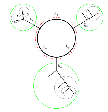
Figure 4: The Casimir equations for $n$-point block $\mathcal{F}^{\,(2,\mathfrak{ch})}_{h,\tilde{h},c}(q,{\bf z})$ with a three-leg necklace sub-diagram. The dashed red line symbolizes three Casimir equations associated to the necklace sub-diagram. The green contours indicate three Casimir equations for three internal dimensions of three segments composing the necklace. Each green contour contains smaller grey contours which define Casimir equations for other internal dimensions of planar sub-diagrams attached to the necklace.

As an example, consider inserting two projectors $\mathbb{P}_{\tilde{h}_{\alpha}}$ and $\mathbb{P}_{\tilde{h}_{\beta}}$ into the $n$-point matrix element

$$\operatorname{Tr}_{\tilde{h}_{1}}\left[q^{L_{0}}\mathcal{O}_{1}\ldots\mathcal{O}_{i-1}\mathbb{P}_{\tilde{h}_{\alpha}}\mathcal{O}_{i}\ldots\mathcal{O}_{j-1}\mathbb{P}_{\tilde{h}_{\beta}}\mathcal{O}_{j}\ldots\mathcal{O}_{n}\right]\,,\qquad j>i\;,$$ (5.3)

that splits a string of $n$ operators into three subgroups, each of which can be further fused by means of OPEs down to a single operator for each subgroup as

$$\operatorname{Tr}_{\tilde{h}_{1}}\left[q^{L_{0}}\tilde{\mathcal{O}}_{s}\,\mathbb{P}_{\tilde{h}_{\alpha}}\tilde{\mathcal{O}}_{t}\,\mathbb{P}_{\tilde{h}_{\beta}}\tilde{\mathcal{O}}_{u}\right],$$ (5.4)

where $\tilde{\mathcal{O}}$ have dimensions $\tilde{h}_{s},\tilde{h}_{t},\tilde{h}_{u}$ and result from particular OPE orderings in each subgroup. In this way we obtain a torus block with a necklace sub-diagram having three legs connected to particular planar diagrams. Following the notation of Section 2.2 this block is denoted $\mathcal{F}^{\,(2,\mathfrak{ch})}_{h,\tilde{h},c}(q,{\bf z})$, where $\mathfrak{ch}$ describes OPE orderings in the three operator groups.

Then, using the relation (5.1) we arrive at the following Casimir equations in the necklace sub-diagram

$$\begin{array}[]{c}\mathcal{C}_{2}[n,1]\,\mathcal{F}^{\,(2,\mathfrak{ch})}_{h,\tilde{h},c}(q,{\bf z})=-\tilde{h}_{1}(\tilde{h}_{1}-1)\,\mathcal{F}^{\,(2,\mathfrak{ch})}_{h,\tilde{h},c}(q,{\bf z})\,,\vspace{2mm}\\ \displaystyle\par\mathcal{C}_{2}[n,i]\,\mathcal{F}^{\,(2,\mathfrak{ch})}_{h,\tilde{h},c}(q,{\bf z})=-\tilde{h}_{\alpha}(\tilde{h}_{\alpha}-1)\,\mathcal{F}^{\,(2,\mathfrak{ch})}_{h,\tilde{h},c}(q,{\bf z})\,,\vspace{2mm}\\ \displaystyle\mathcal{C}_{2}[n,j]\,\mathcal{F}^{\,(2,\mathfrak{ch})}_{h,\tilde{h},c}(q,{\bf z})=-\tilde{h}_{\beta}(\tilde{h}_{\beta}-1)\,\mathcal{F}^{\,(2,\mathfrak{ch})}_{h,\tilde{h},c}(q,{\bf z})\,,\end{array}$$ (5.5)

along with the plane Casimir equations describing OPE orderings $\mathfrak{ch}$ in each of three operator groups

$$\begin{array}[]{l}\displaystyle\tilde{\mathbb{C}}_{2}[1:i-1]\,\mathcal{F}^{\,(2,\mathfrak{ch})}_{h,\tilde{h},c}(q,{\bf z})=-\tilde{h}_{s}(\tilde{h}_{s}-1)\,\mathcal{F}^{\,(2,\mathfrak{ch})}_{h,\tilde{h},c}(q,{\bf z})\,,\vspace{2mm}\\ \displaystyle\tilde{\mathbb{C}}_{2}[i:j-1]\,\mathcal{F}^{\,(2,\mathfrak{ch})}_{h,\tilde{h},c}(q,{\bf z})=-\tilde{h}_{t}(\tilde{h}_{t}-1)\,\mathcal{F}^{\,(2,\mathfrak{ch})}_{h,\tilde{h},c}(q,{\bf z})\,,\vspace{2mm}\\ \displaystyle\tilde{\mathbb{C}}_{2}[j:n]\,\mathcal{F}^{\,(2,\mathfrak{ch})}_{h,\tilde{h},c}(q,{\bf z})=-\tilde{h}_{u}(\tilde{h}_{u}-1)\,\mathcal{F}^{\,(2,\mathfrak{ch})}_{h,\tilde{h},c}(q,{\bf z})\,,\end{array}$$ (5.6)

where similar to (4.5) we introduced the plane Casimir operators

$$\tilde{\mathbb{C}}_{2}[a:b]=\mathbb{L}_{1}\mathbb{L}_{-1}+\mathbb{L}_{0}-(\mathbb{L}_{0})^{2}\,,\qquad\quad\mathbb{L}_{m}=\displaystyle\sum_{k=a}^{b}\mathcal{L}^{(k)}_{m}\,,\quad m=0,\pm 1\,.$$ (5.7)

Of course, this equation system (5.5)-(5.6) is not complete because one has to add Casimir equations describing a particular channel in each of three groups of operators. This can be schematically written as

$$\tilde{\mathbb{C}}_{2}[A:B]\,\mathcal{F}^{\,(2,\mathfrak{ch})}_{h,\tilde{h},c}(q,{\bf z})=-\tilde{h}_{C}(\tilde{h}_{C}-1)\,\mathcal{F}^{\,(2,\mathfrak{ch})}_{h,\tilde{h},c}(q,{\bf z})\,,$$ (5.8)

where $A,B$ are possible labels of primary operators in each subgroup of operators which on fig. 4 correspond to the contours painted in grey, $\tilde{h}_{C}$ stands for an intermediate dimension of the line crossed by a given contour.

The generalization to any number of projectors (legs of the necklace sub-diagram) is obvious. In the case of $n$-point global torus in the OPE channel (see fig. 2 (a)) the above Casimir equations reproduce those ones given in [18].

6 Conclusion and outlooks

In this paper we elaborated on the conformal block decomposition in the torus CFT₂ and recognized the essential role of the necklace channel in building torus conformal blocks in general channels. We explicitly found the Casimir equations for the multipoint global torus block in the necklace channel (3.15). The resulting PDE system is given by 2nd order differential operators both in the modular parameter and local coordinates. The conformal blocks diagonalize these operators with eigenvalues $-\tilde{h}(\tilde{h}-1)$ defined by dimensions of exchange channels. We have also presented the Casimir equations for global torus blocks in any channel.

In particular, the limiting $q\rightarrow 0$ torus blocks with $n$ points in the necklace channel are recognized as plane blocks with $(n+2)$ points in the comb channel. Such an identification can be justified by simple counting of independent variables. The $n$-point torus block depends on $(n-1)$ variables because of global $u(1)$ symmetry. At the same time, the $(n+2)$-point plane block depends on the same $(n-1)$ variables because originally it depends on $(n+2)$ variables but 3 points can be fixed by the global $sl(2,\mathbb{R})$ symmetry. There is also a simple geometric argument underlying this relation: cutting a necklace diagram yields a comb diagram. As a by-product, we obtained the plane Casimir equations as explicit 2nd order differential operators in given coordinates and conformal blocks are their eigenfunctions (4.10).

Our study of global torus conformal blocks was partly motivated by Wilson network realization of conformal blocks in the context of AdS₃/CFT₂ correspondence [48, 49, 50, 18, 51, 52, 53, 54, 55]. On the other hand, semiclassical heavy-light torus blocks dual to geodesic networks in the thermal AdS₃ can be obtained from the large-$h$ (“heavy-light”) expansion of global torus blocks [31, 32, 33, 56]. The Casimir approach could be useful here, see e.g. [18].

Also, from the AdS₃/CFT₂ perspective it would be useful to study $\mathcal{N}=1$ supersymmetric extensions of the Casimir approach for $n$-point superblocks similar to the case of 1-point torus superblocks [27].

Acknowledgements.

Our work was supported by the Foundation for the Advancement of Theoretical Physics and Mathematics “BASIS”.

Appendix A Derivation of the torus Casimir equations for 2-point blocks

In what follows we explicitly derive the Casimir equations in the case $n=2$ and analyze their limits $n=2\to n=1$ at any $q$ and $q\to 0$ at $n=2$.

Derivation of 2-point Casimir equations.

In the 2-point case, the Casimir irreducibility conditions (3.10) are given by two relations

$$\begin{array}[]{c}\displaystyle 1)\;\;\operatorname{Tr}_{\tilde{h}_{1}}[\text{C}_{2}q^{L_{0}}\mathcal{O}_{1}\mathbb{P}_{\tilde{h}_{2}}\mathcal{O}_{2}]=-\tilde{h}_{1}(\tilde{h}_{1}-1)\mathcal{F}_{h,\tilde{h}}\,,\vspace{2mm}\\ \displaystyle 2)\;\;\operatorname{Tr}_{\tilde{h}_{1}}[q^{L_{0}}\mathcal{O}_{1}\mathbb{P}_{\tilde{h}_{2}}\text{C}_{2}\,\mathcal{O}_{2}]=-\tilde{h}_{2}(\tilde{h}_{2}-1)\mathcal{F}_{h,\tilde{h}}\,.\end{array}$$ (A.1)

In order to represent (A.1) as the eigenvalue equations for the 2-point block function $\mathcal{F}_{h,\tilde{h}}$ in the necklace channel (2.11) one substitutes the Casimir operator $\operatorname{C_{2}}=L_{1}L_{-1}-L_{0}-L_{0}^{2}$ (3.9) into the both relations. Each of the three terms in $\operatorname{C_{2}}$ is to be treated separately.

Let us begin with the first relation in (A.1) and consider the term $L_{1}L_{-1}$. The trick is to commute $L_{-1}$ to the right to obtain the following relation

$$\begin{split}\operatorname{Tr}_{\tilde{h}_{1}}[L_{1}L_{-1}q^{L_{0}}\mathcal{O}_{1}\mathbb{P}_{\tilde{h}_{2}}\mathcal{O}_{2}]&=\frac{1}{q}\operatorname{Tr}_{\tilde{h}_{1}}[L_{1}q^{L_{0}}L_{-1}\mathcal{O}_{1}\mathbb{P}_{\tilde{h}_{2}}\mathcal{O}_{2}]=\\ &=\frac{1}{q}\mathcal{L}_{-1}^{(1)}\operatorname{Tr}_{\tilde{h}_{1}}[L_{1}q^{L_{0}}\mathcal{O}_{1}\mathbb{P}_{\tilde{h}_{2}}\mathcal{O}_{2}]+\frac{1}{q}\operatorname{Tr}_{\tilde{h}_{1}}[L_{1}q^{L_{0}}\mathcal{O}_{1}\mathbb{P}_{\tilde{h}_{2}}L_{-1}\mathcal{O}_{2}]\,,\end{split}$$ (A.2)

where we used $L_{n}q^{L_{0}}=q^{L_{0}+n}L_{n}$, $L_{n}\mathbb{P}=\mathbb{P}L_{n}$, and $[L_{n},\mathcal{O}_{i}(z_{i})]=\mathcal{L}_{n}^{(i)}\mathcal{O}_{i}(z_{i})$ (2.4). Commuting $L_{-1}$ with $\mathcal{O}_{2}$ in the last trace in (A.2), using the cyclic property of the trace and then commuting operators $L_{\pm 1}$, we obtain

$$\begin{array}[]{l}\displaystyle\operatorname{Tr}_{\tilde{h}_{1}}[L_{1}L_{-1}q^{L_{0}}\mathcal{O}_{1}\mathbb{P}_{\tilde{h}_{2}}\mathcal{O}_{2}]=\frac{1}{q}(\mathcal{L}_{-1}^{(1)}+\mathcal{L}_{-1}^{(2)})\operatorname{Tr}_{\tilde{h}_{1}}[L_{1}q^{L_{0}}\mathcal{O}_{1}\mathbb{P}_{\tilde{h}_{2}}\mathcal{O}_{2}]\vspace{2mm}\\ \displaystyle\hskip 122.34685pt-\frac{2}{q}\operatorname{Tr}_{\tilde{h}_{1}}[L_{0}q^{L_{0}}\mathcal{O}_{1}\mathbb{P}_{\tilde{h}_{2}}\mathcal{O}_{2}]+\frac{1}{q}\operatorname{Tr}_{\tilde{h}_{1}}[L_{1}L_{-1}q^{L_{0}}\mathcal{O}_{1}\mathbb{P}_{\tilde{h}_{2}}\mathcal{O}_{2}]\,.\end{array}$$ (A.3)

The last step is to calculate the trace $\operatorname{Tr}_{\tilde{h}_{1}}[L_{1}q^{L_{0}}\mathcal{O}_{1}\mathbb{P}_{\tilde{h}_{2}}\mathcal{O}_{2}]$ in the first line of (A.3). Using the same procedure one finds

$$\begin{split}\operatorname{Tr}_{\tilde{h}_{1}}[L_{1}q^{L_{0}}\mathcal{O}_{1}\mathbb{P}_{\tilde{h}_{2}}\mathcal{O}_{2}]&=q\left(\mathcal{L}_{1}^{(1)}+\mathcal{L}_{1}^{(2)}\right)\mathcal{F}_{h,\tilde{h}}+q\operatorname{Tr}_{\tilde{h}_{1}}[q^{L_{0}}\mathcal{O}_{1}\mathbb{P}_{\tilde{h}_{2}}\mathcal{O}_{2}L_{1}]\,.\end{split}$$ (A.4)

By the cyclic property of the trace the last term is similar to the left-hand side term. Substituting it back into (A.3) one obtains

$$\begin{split}\operatorname{Tr}_{\tilde{h}_{1}}[L_{1}L_{-1}q^{L_{0}}\mathcal{O}_{1}\mathbb{P}_{\tilde{h}_{2}}\mathcal{O}_{2}]&=\frac{2}{1-q}q\partial_{q}\mathcal{F}_{h,\tilde{h}}-\frac{q}{(1-q)^{2}}\left(\mathcal{L}_{-1}^{(1)}+\mathcal{L}_{-1}^{(2)}\right)\left(\mathcal{L}_{1}^{(1)}+\mathcal{L}_{1}^{(2)}\right)\mathcal{F}_{h,\tilde{h}}\,.\end{split}$$ (A.5)

Now, $L_{0}$ and $L_{0}^{2}$ terms in the Casimir operator are calculated by using the following obvious relations

$$\operatorname{Tr}_{\tilde{h}_{1}}[L_{0}q^{L_{0}}\mathcal{O}_{1}\mathbb{P}_{\tilde{h}_{2}}\mathcal{O}_{2}]=q\partial_{q}\mathcal{F}_{h,\tilde{h}}\,,\qquad\operatorname{Tr}_{\tilde{h}_{1}}[L^{2}_{0}q^{L_{0}}\mathcal{O}_{1}\mathbb{P}_{\tilde{h}_{2}}\mathcal{O}_{2}]=(q\partial_{q})^{2}\mathcal{F}_{h,\tilde{h}}\,.$$ (A.6)

Finally, the first Casimir equation is cast into the form

$$\begin{split}\left[-q^{2}\partial_{q}^{2}+\frac{2q}{1-q}q\partial_{q}-\frac{q}{(1-q)^{2}}\left(\mathcal{L}_{-1}^{(1)}+\mathcal{L}_{-1}^{(2)}\right)\left(\mathcal{L}_{1}^{(1)}+\mathcal{L}_{1}^{(2)}\right)\right]\mathcal{F}_{h,\tilde{h}}=-\tilde{h}_{1}(\tilde{h}_{1}-1)\mathcal{F}_{h,\tilde{h}}\,,\end{split}$$ (A.7)

which is now the eigenvalue equation for $\mathcal{F}_{h,\tilde{h}}$. This is the first equation in (3.11) at $n=2$.

The same procedure applies to the second relation in (A.1). Isolating the term $L_{1}L_{-1}$ in the Casimir operator (3.9) one obtains

$$\begin{split}\operatorname{Tr}_{\tilde{h}_{1}}[q^{L_{0}}\mathcal{O}_{1}\mathbb{P}_{\tilde{h}_{2}}L_{1}L_{-1}\mathcal{O}_{2}]&=\frac{1}{q}(\mathcal{L}_{-1}^{(1)}+q\mathcal{L}_{-1}^{(2)})\operatorname{Tr}_{\tilde{h}_{1}}[q^{L_{0}}\mathcal{O}_{1}\mathbb{P}_{\tilde{h}_{2}}L_{1}\mathcal{O}_{2}]-\\ &-\frac{2}{q}\operatorname{Tr}_{\tilde{h}_{1}}[q^{L_{0}}\mathcal{O}_{1}\mathbb{P}_{\tilde{h}_{2}}L_{0}\mathcal{O}_{2}]+\frac{1}{q}\operatorname{Tr}_{\tilde{h}_{1}}[q^{L_{0}}\mathcal{O}_{1}\mathbb{P}_{\tilde{h}_{2}}L_{1}L_{-1}\mathcal{O}_{2}]\,,\end{split}$$ (A.8)

where first and second traces on the right-hand side can be cast into the form

$$\begin{array}[]{l}\displaystyle\operatorname{Tr}_{\tilde{h}_{1}}[q^{L_{0}}\mathcal{O}_{1}\mathbb{P}_{\tilde{h}_{2}}L_{1}\mathcal{O}_{2}]=\frac{1}{1-q}\left(\mathcal{L}_{1}^{(2)}+q\mathcal{L}_{1}^{(1)}\right)\mathcal{F}_{h,\tilde{h}}\,,\vspace{2mm}\\ \displaystyle\operatorname{Tr}_{\tilde{h}_{1}}[q^{L_{0}}\mathcal{O}_{1}\mathbb{P}_{\tilde{h}_{2}}L_{0}\mathcal{O}_{2}]=\mathcal{L}_{0}^{(2)}\mathcal{F}_{h,\tilde{h}}+q\partial_{q}\mathcal{F}_{h,\tilde{h}}\,.\end{array}$$ (A.9)

Substituting these expressions into (A.8) yields

$$\begin{split}\operatorname{Tr}_{\tilde{h}_{1}}[q^{L_{0}}\mathcal{O}_{1}\mathbb{P}_{\tilde{h}_{2}}L_{1}L_{-1}\mathcal{O}_{2}]&=\frac{2}{(1-q)}q\partial_{q}\mathcal{F}_{h,\tilde{h}}+\frac{2}{(1-q)}\mathcal{L}_{0}^{(2)}\mathcal{F}_{h,\tilde{h}}-\\ &-\frac{1}{(1-q)^{2}}\left(\mathcal{L}_{-1}^{(1)}+q\mathcal{L}_{-1}^{(2)}\right)\left(\mathcal{L}_{1}^{(2)}+q\mathcal{L}_{1}^{(1)}\right)\mathcal{F}_{h,\tilde{h}}\,.\end{split}$$ (A.10)

Using (A.9) one derives the last term in Casimir operator (3.9) as

$$\begin{split}\operatorname{Tr}_{\tilde{h}_{1}}[q^{L_{0}}\mathcal{O}_{1}\mathbb{P}_{\tilde{h}_{2}}L_{0}^{2}\mathcal{O}_{2}]=\left(\mathcal{L}_{0}^{(2)}\right)^{2}\mathcal{F}_{h,\tilde{h}}+2\mathcal{L}_{0}^{(2)}q\partial_{q}\mathcal{F}_{h,\tilde{h}}+q\partial_{q}(q\partial_{q}\mathcal{F}_{h,\tilde{h}})\,.\end{split}$$ (A.11)

Substituting (A.10), (A.9), (A.11) into (A.1) one finally obtains

$$\begin{array}[]{l}\displaystyle\left[-q^{2}\partial_{q}^{2}+\frac{2q}{1-q}q\partial_{q}-\frac{1}{(1-q)^{2}}\left(\mathcal{L}_{-1}^{(1)}+q\mathcal{L}_{-1}^{(2)}\right)\left(\mathcal{L}_{1}^{(2)}+q\mathcal{L}_{1}^{(1)}\right)\right.\vspace{2mm}\\ \displaystyle\hskip 113.81102pt\left.+\frac{1+q}{1-q}\mathcal{L}_{0}^{(2)}-\left(\mathcal{L}_{0}^{(2)}\right)^{2}-2\mathcal{L}_{0}^{(2)}q\partial_{q}\right]\mathcal{F}_{h,\tilde{h}}=-\tilde{h}_{2}(\tilde{h}_{2}-1)\mathcal{F}_{h,\tilde{h}}\,,\end{array}$$ (A.12)

which is the second equation in (3.11) at $n=2$. It is straightforward to check that the 2-point torus block function (3.2) does solve the Casimir equation system (A.7) and (A.12). The same procedure in the $n$-point case yields the Casimir system (3.11).

Reduction to the 1-point Casimir equation.

Let us show that the 2-point Casimir equations (A.7) and (A.12) are reduced to the 1-point Casimir equation [18]. To this end, we choose the second primary operator to be the identity operator, $\mathcal{O}_{2}(z_{2})=\mathbb{I}$, i.e. $h_{2}=0$. It follows that the intermediate dimensions must be equated, $\tilde{h}_{1}=\tilde{h}_{2}$.

The 2-point conformal block $\mathcal{F}_{h,\tilde{h}}\equiv\mathcal{F}_{h_{1}h_{2},\tilde{h}_{1}\tilde{h}_{2}}$ satisfies the Ward identity (3.12): $(\mathcal{L}_{0}^{(1)}+\mathcal{L}_{0}^{(2)})\mathcal{F}_{h_{1}h_{2},\tilde{h}_{1}\tilde{h}_{2}}=0$, which by using (2.4) takes the form

$$\left(h_{1}+h_{2}+z_{1}\partial_{1}+z_{2}\partial_{2}\right)\mathcal{F}_{h_{1}h_{2},\tilde{h}_{1}\tilde{h}_{2}}=0\,.$$ (A.13)

On the other hand, the $1$-point block $\mathcal{F}_{h_{1},\tilde{h}_{1}}\equiv\mathcal{F}_{h_{1}h_{2},\tilde{h}_{1}\tilde{h}_{2}}\big{|}_{h_{2}=0,\tilde{h}_{2}=\tilde{h}_{1}}$ satisfies the Ward identity $\mathcal{L}_{0}^{(1)}\mathcal{F}_{h_{1},\tilde{h}_{1}}=0$. Then, together with the condition $h_{2}=0$, equation (A.13) gives

$$\partial_{2}\mathcal{F}_{h_{1},\tilde{h}_{1}}=0\,.$$ (A.14)

Thus, the first Casimir equation (A.7) takes the form [18]

$$\left[-q^{2}\partial_{q}^{2}+\frac{2q}{1-q}q\partial_{q}+\frac{q}{(1-q)^{2}}h_{1}(h_{1}-1)\right]\mathcal{F}_{h_{1},\tilde{h}_{1}}=-\tilde{h}_{1}(\tilde{h}_{1}-1)\mathcal{F}_{h_{1},\tilde{h}_{1}}\,.$$ (A.15)

Similarly, using (A.14) and $\tilde{h}_{1}=\tilde{h}_{2}$ one shows that the second Casimir equation (A.12) also reduces to (A.15).

Reduction from the $2$-point torus block to the $4$-point plane block.

Let us illustrate the relation (4.2) for the $2$-point torus block with external dimensions $(h_{1},h_{2})$ and intermediate dimensions $(\tilde{h}_{1},\tilde{h}_{2})$ in the plane limit. Setting $n=j=2$ in (4.3) we find

$$\bigg{[}\tilde{h}_{1}(1-\tilde{h}_{1})-\mathcal{L}_{-1}^{(1)}\mathcal{L}_{1}^{(2)}+(1-2\tilde{h}_{1})\mathcal{L}_{0}^{(2)}-\left(\mathcal{L}_{0}^{(2)}\right)^{2}+\tilde{h}_{2}(\tilde{h}_{2}-1)\bigg{]}\mathcal{F}_{0}(z_{1},z_{2})=0\,.$$ (A.16)

Using (2.4) one directly shows that (A.16) is reduced to the hypergeometric equation and its solution has the following form

$$\mathcal{F}_{0}(z_{1},z_{2})=z_{1}^{-h_{1}}z_{2}^{-h_{2}}\;x^{\tilde{h}_{2}-\tilde{h}_{1}}\;{}_{2}F_{1}\left(\tilde{h}_{2}-\tilde{h}_{1}+h_{1},\tilde{h}_{2}-\tilde{h}_{1}+h_{2},2\tilde{h}_{2}\,\big{|}\,x\right),$$ (A.17)

where $x=z_{2}/z_{1}$. On the other hand, the 4-point plane block is known to be given by the hypergeometric function of external dimensions $(h_{0},h_{1},h_{2},h_{3})$ and intermediate dimension $\tilde{h}$:

$$\begin{array}[]{l}\displaystyle\tilde{\mathcal{F}}(z_{0},z_{1},z_{2},z_{3}|h,\tilde{h})=z_{01}^{-h_{0}-h_{1}}z_{23}^{-h_{2}-h_{3}}z_{02}^{-h_{0}+h_{1}}z_{12}^{h_{0}-h_{1}-h_{2}+h_{3}}z_{13}^{h_{2}-h_{3}}\vspace{2mm}\\ \displaystyle\hskip 85.35826pt\times\,\eta^{\tilde{h}}(1-\eta)^{h_{2}-h_{3}-h_{0}+h_{1}}\;{}_{2}F_{1}\left(\tilde{h}-h_{0}+h_{1},\tilde{h}+h_{2}-h_{3},2\tilde{h}\,\big{|}\,\eta\right),\end{array}$$ (A.18)

where $z_{ij}\equiv z_{i}-z_{j}$ and the cross-ratio $\eta=(z_{01}z_{23})/(z_{02}z_{13})$. Then, (A.17) is indeed related to (A.18) by (4.2) provided that the external/intermediate dimensions in (A.18) are chosen as $(\tilde{h}_{1},h_{1},h_{2},\tilde{h}_{1})$ and $\tilde{h}_{2}$.

Appendix B Explicit expressions for lower-point global torus block

Here we collect a few explicit block functions.

• The $1$-point block reads [23]

  $$\mathcal{F}_{h,\tilde{h}}(q,z)=z^{-h}\sum^{\infty}_{n=0}\frac{\tau_{n,n}(\tilde{h},h,\tilde{h})}{n!(2\tilde{h})_{n}}q^{\tilde{h}+n},$$ (B.1)

  where $\tau$-coefficients are given by (3.3).

• The $2$-point block in the necklace channel is (here and below $x_{j}=z_{j}/z_{j-1}$) [19]

  $$\mathcal{F}_{h_{1}h_{2},\tilde{h}_{1},\tilde{h}_{2}}(q,z_{1},z_{2})=z^{-h_{1}}_{1}z^{-h_{2}}_{2}\sum^{\infty}_{n,m=0}\frac{\tau_{n,m}(\tilde{h}_{1},h_{1},\tilde{h}_{2})\tau_{m,n}(\tilde{h}_{2},h_{2},\tilde{h}_{1})}{n!m!(2\tilde{h}_{1})_{n}(2\tilde{h}_{2})_{m}}q^{\tilde{h}_{1}+n}x_{2}^{\tilde{h}_{2}-\tilde{h}_{1}+m-n}.$$ (B.2)

• Using (B.1) one can find the 2-point and 3-point OPE blocks shown on fig. 3 (c) and (f) given by (3.6) and (3.7), respectively [18, 19]:

  $$\mathcal{F}^{\,(0,\mathfrak{ch}_{1})}_{h_{1}h_{2},\tilde{h}_{1}\tilde{h}_{2}}(q,z_{1},z_{2})=z^{-h_{1}}_{1}z^{-h_{2}}_{2}\sum^{\infty}_{n,m=0}\frac{\tau_{n,n}(\tilde{h}_{1},\tilde{h}_{2},\tilde{h}_{1})\sigma_{m}}{n!m!(2\tilde{h}_{1})_{n}(2\tilde{h}_{2})_{m}}q^{\tilde{h}_{1}+n}(1-x_{2})^{\tilde{h}_{2}-h_{1}-h_{2}+m}x^{h_{2}-\tilde{h}_{2}-m}_{2},$$ (B.3)

  where $\sigma_{m}=(-1)^{m}(\tilde{h}_{2})_{m}(\tilde{h}_{2}+h_{1}-h_{2})_{m}$, and

  $$\begin{array}[]{c}\mathcal{F}^{\,(0,\mathfrak{ch}_{2})}_{h_{1}h_{2}h_{3},\tilde{h}_{1}\tilde{h}_{2}\tilde{h}_{3}}(q,z_{1},z_{2},z_{3})=z^{-h_{1}}_{1}z^{-h_{2}}_{2}z^{-h_{3}}_{3}\displaystyle\sum^{\infty}_{n,m,k=0}\frac{\tau_{n,n}(\tilde{h}_{1},\tilde{h}_{2},\tilde{h}_{1})\sigma_{m,k}}{n!m!k!(2\tilde{h}_{1})_{n}(2\tilde{h}_{2})_{m}(2\tilde{h}_{3})_{k}}q^{\tilde{h}_{1}+n}\\ \times(1-x_{2})^{\tilde{h}_{3}-h_{1}-h_{2}+k}(1-x_{3})^{\tilde{h}_{2}-h_{3}-\tilde{h}_{3}+m-k}x^{h_{2}-\tilde{h}_{3}-k}_{2}x^{-\tilde{h}_{2}-m}_{3},\end{array}$$ (B.4)

  where $\sigma_{m,k}=(-1)^{m+k}(\tilde{h}_{2})_{m}(\tilde{h}_{3}+h_{1}-h_{2})_{k}(\tilde{h}_{2}+\tilde{h}_{3}-h_{3}+m)_{k}(\tilde{h}_{2}+\tilde{h}_{3}-h_{3})_{m}$.

• The mixed channel 3-point block (see fig. 3 (e)) is determined by (B.2) and (3.8)

  $$\begin{array}[]{c}\mathcal{F}^{\,(1,\mathfrak{ch}_{1})}_{h_{1}h_{2}h_{3},\tilde{h}_{1}\tilde{h}_{2}\tilde{h}_{3}}(q,z_{1},z_{2},z_{3})=z^{-h_{1}}_{1}z^{-h_{2}}_{2}z^{-h_{3}}_{3}\displaystyle\sum^{\infty}_{m,n,k=0}\frac{\tau_{m,k}(\tilde{h}_{1},\tilde{h}_{3},\tilde{h}_{2})\tau_{k,m}(\tilde{h}_{2},h_{3},\tilde{h}_{1})\sigma_{m,n,k}}{m!n!k!(2\tilde{h}_{1})_{m}(2\tilde{h}_{2})_{k}(2\tilde{h}_{3})_{n}}\\ \displaystyle\times q^{\tilde{h}_{1}+m}(1-x_{2})^{\tilde{h}_{3}-h_{1}-h_{2}+n}x^{h_{2}-\tilde{h}_{3}}_{2}x_{3}^{\tilde{h}_{2}-\tilde{h}_{1}+k-m}\;,\end{array}$$ (B.5)

  where $\sigma_{m,n,k}=(-1)^{n}(\tilde{h}_{1}-\tilde{h}_{3}-\tilde{h}_{2}+m-k-n+1)_{n}(\tilde{h}_{3}+h_{2}-h_{1})_{n}$. It is a straightforward to check that this function satisfies the Casimir equations in the mixed channel (5.5)-(5.6).

References

- [1] A. Belavin, A. M. Polyakov and A. Zamolodchikov, Infinite Conformal Symmetry in Two-Dimensional Quantum Field Theory, Nucl.Phys. B241 (1984) 333–380.
- [2] E. P. Verlinde, Fusion Rules and Modular Transformations in 2D Conformal Field Theory, Nucl. Phys. B 300 (1988) 360–376.
- [3] D. Poland, S. Rychkov and A. Vichi, The Conformal Bootstrap: Theory, Numerical Techniques, and Applications, Rev. Mod. Phys. 91 (2019) 015002, [1805.04405].
- [4] S. Collier, Y.-H. Lin and X. Yin, Modular Bootstrap Revisited, JHEP 09 (2018) 061, [1608.06241].
- [5] T. Hartman, D. Mazac, D. Simmons-Duffin and A. Zhiboedov, Snowmass White Paper: The Analytic Conformal Bootstrap, in 2022 Snowmass Summer Study, 2, 2022. 2202.11012.
- [6] A. Bissi, A. Sinha and X. Zhou, Selected Topics in Analytic Conformal Bootstrap: A Guided Journey, 2202.08475.
- [7] T. Hartman, Entanglement Entropy at Large Central Charge, 1303.6955.
- [8] A. L. Fitzpatrick, J. Kaplan and M. T. Walters, Universality of Long-Distance AdS Physics from the CFT Bootstrap, JHEP 08 (2014) 145, [1403.6829].
- [9] E. Hijano, P. Kraus and R. Snively, Worldline approach to semi-classical conformal blocks, JHEP 07 (2015) 131, [1501.02260].
- [10] K. B. Alkalaev and V. A. Belavin, Classical conformal blocks via AdS/CFT correspondence, JHEP 08 (2015) 049, [1504.05943].
- [11] E. Hijano, P. Kraus, E. Perlmutter and R. Snively, Witten Diagrams Revisited: The AdS Geometry of Conformal Blocks, JHEP 01 (2016) 146, [1508.00501].
- [12] E. Hijano, P. Kraus, E. Perlmutter and R. Snively, Semiclassical Virasoro blocks from AdS3 gravity, JHEP 12 (2015) 077, [1508.04987].
- [13] P. Banerjee, S. Datta and R. Sinha, Higher-point conformal blocks and entanglement entropy in heavy states, JHEP 05 (2016) 127, [1601.06794].
- [14] J. L. Cardy, Operator Content of Two-Dimensional Conformally Invariant Theories, Nucl. Phys. B270 (1986) 186–204.
- [15] C. Itzykson and J. B. Zuber, Two-Dimensional Conformal Invariant Theories on a Torus, Nucl. Phys. B 275 (1986) 580–616.
- [16] T. Eguchi and H. Ooguri, Conformal and Current Algebras on General Riemann Surface, Nucl. Phys. B 282 (1987) 308–328.
- [17] M. Cho, S. Collier and X. Yin, Recursive Representations of Arbitrary Virasoro Conformal Blocks, JHEP 04 (2019) 018, [1703.09805].
- [18] P. Kraus, A. Maloney, H. Maxfield, G. S. Ng and J.-q. Wu, Witten Diagrams for Torus Conformal Blocks, JHEP 09 (2017) 149, [1706.00047].
- [19] K. B. Alkalaev and V. A. Belavin, Holographic duals of large-c torus conformal blocks, JHEP 10 (2017) 140, [1707.09311].
- [20] J. Ramos Cabezas, Semiclassical torus blocks in the t-channel, JHEP 08 (2020) 151, [2005.04128].
- [21] M. Gerbershagen, Monodromy methods for torus conformal blocks and entanglement entropy at large central charge, JHEP 08 (2021) 143, [2101.11642].
- [22] J. D. Brown and M. Henneaux, Central Charges in the Canonical Realization of Asymptotic Symmetries: An Example from Three-Dimensional Gravity, Commun.Math.Phys. 104 (1986) 207–226.
- [23] L. Hadasz, Z. Jaskolski and P. Suchanek, Recursive representation of the torus 1-point conformal block, JHEP 01 (2010) 063, [0911.2353].
- [24] F. A. Dolan and H. Osborn, Conformal partial waves and the operator product expansion, Nucl. Phys. B 678 (2004) 491–507, [hep-th/0309180].
- [25] F. Dolan and H. Osborn, Conformal Partial Waves: Further Mathematical Results, 1108.6194.
- [26] Y. Gobeil, A. Maloney, G. S. Ng and J.-q. Wu, Thermal Conformal Blocks, SciPost Phys. 7 (2019) 015, [1802.10537].
- [27] K. Alkalaev and V. Belavin, Large- superconformal torus blocks, JHEP 08 (2018) 042, [1805.12585].
- [28] V. Rosenhaus, Multipoint Conformal Blocks in the Comb Channel, JHEP 02 (2019) 142, [1810.03244].
- [29] J.-F. Fortin, W. Ma and W. Skiba, Higher-Point Conformal Blocks in the Comb Channel, JHEP 07 (2020) 213, [1911.11046].
- [30] A. Zamolodchikov, Two-dimensional conformal symmetry and critical four-spin correlation functions in the Ashkin-Teller model, Zh. Eksp. Teor. Fiz. 90 (1986) 1808–1818.
- [31] A. L. Fitzpatrick, J. Kaplan and M. T. Walters, Virasoro Conformal Blocks and Thermality from Classical Background Fields, JHEP 11 (2015) 200, [1501.05315].
- [32] K. B. Alkalaev and V. A. Belavin, From global to heavy-light: 5-point conformal blocks, JHEP 03 (2016) 184, [1512.07627].
- [33] K. B. Alkalaev, R. V. Geiko and V. A. Rappoport, Various semiclassical limits of torus conformal blocks, JHEP 04 (2017) 070, [1612.05891].
- [34] E. Perlmutter, Virasoro conformal blocks in closed form, JHEP 08 (2015) 088, [1502.07742].
- [35] G. Felder and R. Silvotti, Modular Covariance of Minimal Model Correlation Functions, Commun. Math. Phys. 123 (1989) 1–15.
- [36] P. Kraus and A. Maloney, A Cardy formula for three-point coefficients or how the black hole got its spots, JHEP 05 (2017) 160, [1608.03284].
- [37] E. M. Brehm, D. Das and S. Datta, Probing thermality beyond the diagonal, Phys. Rev. D 98 (2018) 126015, [1804.07924].
- [38] P. Menotti, Torus classical conformal blocks, Mod. Phys. Lett. A33 (2018) 1850166, [1805.07788].
- [39] M. Piatek, Classical torus conformal block, twisted superpotential and the accessory parameter of Lame equation, JHEP 03 (2014) 124, [1309.7672].
- [40] J.-F. Fortin, W.-J. Ma and W. Skiba, All Global One- and Two-Dimensional Higher-Point Conformal Blocks, 2009.07674.
- [41] J.-F. Fortin, W.-J. Ma and W. Skiba, Six-point conformal blocks in the snowflake channel, JHEP 11 (2020) 147, [2004.02824].
- [42] J.-F. Fortin, W.-J. Ma and W. Skiba, Seven-point conformal blocks in the extended snowflake channel and beyond, Phys. Rev. D 102 (2020) 125007, [2006.13964].
- [43] D. Simmons-Duffin, The Conformal Bootstrap, in Theoretical Advanced Study Institute in Elementary Particle Physics: New Frontiers in Fields and Strings, pp. 1–74, 2017. 1602.07982.
- [44] R. Blumenhagen and E. Plauschinn, Introduction to Conformal Field Theory: With Applications to String Theory, Springer (2009) .
- [45] J. D. Qualls, Lectures on Conformal Field Theory, 1511.04074.
- [46] D. Simmons-Duffin, Projectors, Shadows, and Conformal Blocks, JHEP 04 (2014) 146, [1204.3894].
- [47] M. Isachenkov and V. Schomerus, Superintegrability of -dimensional Conformal Blocks, Phys. Rev. Lett. 117 (2016) 071602, [1602.01858].
- [48] A. Bhatta, P. Raman and N. V. Suryanarayana, Holographic Conformal Partial Waves as Gravitational Open Wilson Networks, JHEP 06 (2016) 119, [1602.02962].
- [49] A. L. Fitzpatrick, J. Kaplan, D. Li and J. Wang, Exact Virasoro Blocks from Wilson Lines and Background-Independent Operators, JHEP 07 (2017) 092, [1612.06385].
- [50] M. Besken, A. Hegde, E. Hijano and P. Kraus, Holographic conformal blocks from interacting Wilson lines, 1603.07317.
- [51] Y. Hikida and T. Uetoko, Conformal blocks from Wilson lines with loop corrections, Phys. Rev. D 97 (2018) 086014, [1801.08549].
- [52] Y. Hikida and T. Uetoko, Superconformal blocks from Wilson lines with loop corrections, JHEP 08 (2018) 101, [1806.05836].
- [53] K. Alkalaev and V. Belavin, More on Wilson toroidal networks and torus blocks, JHEP 11 (2020) 121, [2007.10494].
- [54] A. Castro, P. Sabella-Garnier and C. Zukowski, Gravitational Wilson Lines in 3D de Sitter, JHEP 07 (2020) 202, [2001.09998].
- [55] V. Belavin and J. R. Cabezas, Wilson lines construction of conformal blocks, 2204.12149.
- [56] K. B. Alkalaev and V. A. Belavin, Holographic interpretation of 1-point toroidal block in the semiclassical limit, JHEP 06 (2016) 183, [1603.08440].