Abstract: Visual and scalar-field (e.g., chemical) sensing are two of the options robot teams can use to perceive their environments when performing tasks. We give the first comparison of the computational characteristic of visual and scalar-field sensing, phrased in terms of the computational complexities of verifying and designing teams of robots to efficiently and robustly perform distributed construction tasks. This is done relative a basic model in which teams of robots with deterministic finite-state controllers operate in a synchronous error-free manner in 2D grid-based environments. Our results show that for both types of sensing, all of our problems are polynomial-time intractable in general and remain intractable under a variety of restrictions on parameters characterizing robot controllers, teams, and environments. That being said, these results also include restricted situations for each of our problems in which those problems are effectively polynomial-time tractable. Though there are some differences, our results suggest that (at least in this stage of our investigation) verification and design problems relative to visual and scalar-field sensing have roughly the same patterns and types of tractability and intractability results.

1 Introduction

“As if I had been totally color-blind before, and suddenly found myself in a world full of color …I had dreamt I was a dog — it was an olfactory dream — and now I awoke to an infinitely redolent world — a world in which all other senses, enhanced as they were, paled before smell.”
— Oliver Sacks, “The Dog Beneath the Skin” [1]

We human beings perceive much of our world by sight, using visible light and binocular vision to determine both the presence and nature of objects in our environment and their distances and orientations relative to ourselves. Visual senses exist that exploit other forms of radiated energy (e.g., infrared light, ultrasound (see [2, Chapters 8 and 9], [3, Sections 2.4 and 2,7], and references). There are also senses such as smell based on the proximal detection of scalar fields. Not greatly developed in modern human beings (but revivable to stunning effect, as shown by the medical student Stephen D. quoted by Sacks), smell is critical in the activities of many creatures (e.g., bacteria following chemical gradients to approach food or flee toxins, moths finding mates by pheromones). Senses also exist that exploit other types of scalar fields (e.g., blue-green bacteria approaching sunlight to optimize photosynthesis, fish using electrical fields to find prey in muddy water, birds navigating using Earth’s magnetic field (see [2, Chapters 6, 7, and 10], [3, Sections 2.2, 2.3, 2.5, and 2.6], and references).

It is perhaps not surprising that when we have built artificial systems, they have first been endowed with visual senses [4, 5] based not only on those seen in nature (e.g., binocular cameras, sonar) but on other forms of radiation as well (e.g., lidar, radar). Much work has also been done on endowing artificial systems with various types of scalar-field-based senses (e.g., the detection and localization of noxious chemical leaks) [6, 7] as well as integrating both types of sensory information to aid in performing tasks (e.g., lidar and GPS in autonomous vehicles).

Visual and scalar-field sensing have different characteristics and thus different advantages and disadvantages. In general, visual sensors are more complex but yield more information (in terms of distance and perceived object characteristics), while scalar-field sensors are simpler but yield less information unless augmented by spatial gradient sensing and the ability to discriminate fine variation in perceived scalar quantities. A finer-grained description of these characteristics would be useful, particularly in applications such as micro- and nano-robotics [8, 9, 10] where conventional types of visual sensing are extremely curtailed or impossible.

Investigations of these issues have previously been done via experiments and simulations [6, 7, 11]. Recent theoretical research [12, 13, 14, 15, 16, 17, 18] complements this work by exploring the computational characteristics of problems associated with the design of robot controllers, teams, and environments for robot teams that perceive using visual and scalar-field senses. This work uses computational [19] and parameterized [20] complexity analysis to characterize those situations in which each of the investigated problems is and is not efficiently solvable, where situations are described in terms of restrictions on sets of one or more aspects characterizing individual robot controllers, robot teams, and operating environments.

It would be of great interest to compare the computational characteristics of visual and scalar-field sensing, as both an aid for robotics researchers in interpreting experimental observations and an alternative perspective on the relative advantages and disadvantages of both kinds of sensing. Characterizations of the computational tractability and intractability of problems are nothing new — indeed, they have been a central part of computer science since the dawn of algorithm design and computational complexity analysis. However, we believe that such work becomes more useful if it also incorporates the following:

1. A focus on determining the mechanisms in problems that interact to produce intractability.

2. A focus on making the results of analyses as well as the techniques by which these results were derived comprehensible to researchers who are not theoretical computer scientists.

Focus (1) implies that the complexity analyses should be done (at least initially) relative to simplified versions of problems that occur in the real world. This is done not only to simplify analysis but also (as in the classic thought experiments of [21]) to allow easier exploration of mechanism interactions in these problems independent of real-world complications. Focus (2) implies that result details (in particular those underlying intractability results) should be part of the presentation of results. This is done to allow robotics researchers to better appreciate the restrictions under which our tractability and intractability results hold and hence more easily collaborate in deriving results for more realistic and useful instances of verification and design problems.

1.1 Previous Work

Various work has been done on the computational complexity of both verifying if a given multi-entity system can perform a task and designing such systems for tasks. The systems so treated include groups of agents [22, 23, 24], robots [25, 26], game-pieces [27], and tiles [28]. Much of this work, e.g. [28, 25, 27, 26], assumes that the entities being moved cannot sense, plan, or move autonomously. In the work where entities do have these abilities, e.g. [22, 23, 24], the formalizations of control mechanisms and environments are very general and powerful (e.g., arbitrary Turing machines or Boolean propositional formulae), rendering both the intractability of these problems unsurprising and the derived results unenlightening with respect to possible restrictions that could yield tractability.

Eight complexity-theoretic papers to date incorporate both autonomous robots and a suitably simple and explicit model of robot architecture and environment [12, 13, 14, 29, 15, 16, 17, 18]. Four of these papers consider navigation tasks performed by robots with deterministic Brooks-style subsumption [13, 15] and finite-state [29, 17] reactive controllers, respectively. The other four consider construction-related tasks performed by robots with deterministic finite-state controllers relative to robot controller and environment design in a given environment where robot controllers are designed from scratch [16, 18], robot team design where teams are designed by selection from a provided library [14, 18], and robot team / environment co-design where robot teams are designed by selection from a provided library [12]. All eight papers use a 2D grid environment model. Seven of these papers have robots that can visually sense the type of any square within a specified Manhattan-distance radius of a robot’s position, with the robots in [17] using single line-of-sight sensors. Only one complexity-theoretic analysis to date has considered environment and robot-team design problems under scalar-field sensing [18]; however, due to conference page limits, no formal proofs of cited results were given.

1.2 Summary of Results

In this paper, we give the first comparison of the computational characteristics of visual and scalar-field sensing. This is phrased in terms of the results of both computational and parameterized complexity analyses of the following five verification and design problems for robot teams and environments:

1. Team / Environment Verification: Does a given team perform a specified task in a given environment?

2. Controller Design by Library Selection: Can a robot controller be constructed from a given library of controller components that allows a team endowed with that controller to perform a specified task in a given environment?

3. Team Design by Library Selection: Can the controllers of the members of a team be selected from a given library of robot controllers such that the resulting team performs a specified task in a given environment?

4. Environment Design: Can an environment be designed such that a given team can perform a specified task in that environment?

5. Team / Environment Co-design by Library Selection: Can the controllers of the members of a team be selected from a given library of robot controllers and an environment be designed such that the resulting team performs a specified task in that environment?

Results for scalar-field sensing are derived relative to a basic model of scalar fields, [18] in which these fields are generated by field-quantities spreading outwards from discrete sources located in the environment. We use the robot team operation and task models proposed in [16] in which teams of robots with finite-state controllers operate in a non-continuous, synchronous, and error-free manner to perform distributed construction tasks [31].

Our results show that for both types of sensing, all of our problems are polynomial-time intractable in general and remain intractable under a variety of restrictions on aspects characterizing robot controllers, teams, and environments, both individually and in many combination and often when aspects are restricted to small constant values. That being said, our results also include restricted situations for each of our problems in which those problems are effectively polynomial-time tractable. Our results show that, though there are some differences, both kinds of sensing have (at least in this stage of our investigation) roughly the same types and patterns of intractability and tractability results.

Before we close out this subsection, clarification is in order regarding the provenance of results reported here. Results for problems (1–5) have been given previously in other papers with proof for visual sensing (Results A.ST.1 and D.ST.1–6 [16]; Result B.ST.1 [29]; Results C.ST.1–3, C.ST.6, and C.ST.7 [14]; Results E.ST.1–6 [12]) and in other papers without proof for scalar-field sensing (Results C.SF.1–7 and D.SF.1–7 [18]). All other results (Result A.SF.1 (Problem (1)); Results B.ST.2–4 and B.SF.1–5 (Problem (2)); Results C.ST.4 and C.ST.5,(Problem (3)); Results E.SF.1–7 (Problem (5)) are new here, as well as the proofs of all results cited previously in [18]. Hence, if one counts the results in [18] as new, there are 19 previous and 32 new results in this paper. Though a number of these new results build on proofs of results described previously, many also involve non-trivial modification of and additions to those previous proofs and hence are not simply incremental extensions of previous work.

1.3 Organization of Paper

This paper is organized as follows. In Section 2, we describe the environment, target structure, robot controller, and robot team models used to formalize our verification and design problems relative to visual and scalar-field sensing. In Section 3, we consider the viable algorithmic options for these problems relative to two popular types of exact and restricted efficient solvability. To allow focus on this comparison and its implications in the main text, all proofs of previously unpublished results are given in an appendix. In Section 4, we discuss the overall implications of our results for our simplified problems and real-world robotics, and propose a metaphor for thinking about comparative computational complexity analyses. Finally, our conclusions and directions for future work are given in Section 5.

2 Formalizing Scalar-field Sensing for Distributed Construction

In this section, we first describe the basic entities in our models (given previously in [16, 18]) of distributed construction relative to visual and scalar-field sensing — namely, environments, structures, individual robots and robot teams. We then formalize the computational problems associated with robot controller, team, and environment design (based on those defined in [12, 14, 16, 18]) that we will analyze in the remainder of this paper.

The basic entities are as follows:

• Environments: Our robots operate in a finite 2D square-based environment $E$ based on a 2D grid $G$; for simplicity, we will assume that there are no obstacles and hence robots can move and fields can propagate freely through any square. Let $E_{i,j}$ denote the square that is in the $i$th column and $j$th row of $E$ such that $E_{1,1}$ is the square in the southwest-most corner of $E$.

  We have two types of environments, square-type and scalar-field, which are associated with visual and scalar-field sensing, respectively. These two types of environments are necessary as the environmental aspects sensed by visual and scalar-field sensing behave in different ways. In a square-type environment, each square in $G$ has a square-type, e.g., grass, gravel, wall, drawn from a set $E_{T}$. An example square-type environment is shown in Figure 1(a). A scalar-field environment has a set of scalar-field instances drawn from a field-set $S$ that are placed within $G$. A scalar field $s\in S$ is defined by a field-quantity $fq$, a field-type, a source-value $s_{s}$ that is a positive real number, and a decay $s_{d}$ that is a non-negative real number. There are two types of fields:

  1. Point-fields that radiate outwards radially from a specified grid-square, and

  2. Edge-fields that radiate outward linearly from a specified grid-edge, which can be North, South, East or West, in the opposite compass direction of the source edge.

  The value of $fq$ for a field-instance $s$ in a square $p$ in scalar-field environment $E$ is $s_{s}-(s_{d}\times z)$, where $z$ is the Manhattan distance between $p$ and the field-source in the case of point-fields and the shortest Manhattan distance between $p$ and the specified grid-edge in the case of edge-fields. As such, our scalar fields are generated by field-quantities spreading outwards from discrete sources in the environment (see Footnote 1). Example point- and edge-fields are shown in Figures 1(b) and 1(c), respectively. Each square in $E$ can have at most one point-field, though each grid-edge may have multiple edge-fields. As there may be multiple instances of fields based on the same field-quantity $fq$ in $E$, the value of $fq$ in a square $p$ in $E$ is the sum of the values of all field-instances based on $fq$ in $E$ at $p$. An example of such an environment summed relative to one edge-field and two point-fields based on the same field-quantity is shown in Figure 1(d).

  

  Figure 1: Example square-type and scalar-field environments (Modified from Figure 1 in [18]). a) A square-type environment based on the square-type set $E_{T}=\{e_{V1},e_{V2},e_{V3},e_{V4},e_{N},e_{S},e_{W},$ $e_{E},e_{M1},e_{M2},e_{M3},e_{T},e_{B}\}$; all blank squares have type $e_{B}$ (adapted from Figure 2 in [14]). b) A scalar-field environment with a point-field based at square $E_{3,3}$ having source-value 1.0 and decay 0.4. c) A scalar-field environment with an East-based edge-field with source-value 2.0 and decay 0.5. d) A scalar-field environment with three fields based on the same field-quantity (a North-based edge-field with source-value 0.3 and decay 0.1; a point-field based at square $E_{4,1}$ with source-value 4.0 and decay 1.0; a point-field based at square $E_{9,4}$ with source-value 2.0 and decay 1.8). The source-region of each field is indicated with a boldfaced box.

  In square-type environments, every square-type set $E_{T}$ contains the special square-types $e_{X}$ (that is used to specify parts of structures) and $e_{robot}$ (that is used to indicate the positions of robots). In scalar-field environments, every field-set $S$ contains special point-fields $s_{X}$ (with source-value 1 and decay-value 0.5 that is used to specify parts of structures) and $s_{robot}$ (with source-value 1 and decay-value 0.5 that is used to indicate the positions of robots).

• Structures: A structure $X$ in an environment $E$ is a two-dimensional pattern of structural elements in an $m\times n$ grid whose location in $E$ is specified relative to the position $p_{X}$ of southwest-most corner of the structure-grid in the environment-grid. The structural elements are squares of type $e_{X}$ and point-fields $s_{X}$ in square-type and scalar-field environments, respectively. An example linear structure is shown in Figure 3.

• Robots: Each robot occupies a square in an environment $E$ and in a basic movement-action can either move exactly one square to the north, south, east or west of its current position or elect to stay at its current position. In square-type environments, a robot can sense the type of any square out to specified Manhattan distance $r$ and modify the type of any square out to Manhattan distance one from the robot’s current position using the predicates $enval()$ and $enmod()$ (see [16] for details); note that the square at Manhattan distance zero (e.g., $r=0$) is the robot’s current position. In this type of environment, square-type modifications correspond to real-world activities such as agents placing construction materials or signs to guide other agents, e.g., “turn right”, “this way to food”, “do not go beyond this point”. Each robot has an associated square-type $e_{robot}$ at its current position.

  In scalar-field environments, a robot can sense both the absolute value of any field-quantity in and the manner in which that quantity changes in any square immediately adjacent to the square in which that robot is currently positioned. These two types of sensing are done using the following predicates:

  1. $fval(fq,rel,val)$, $rel\in\{=,<,>,\leq,\geq\}$, which returns $True$ if $fq~{}rel~{}val$ in the robot’s current position and $False$ otherwise; and

  2. $fgrd(fq,rel,dir)$, $rel\in\{=,<,>,\leq,\geq\}$ and $dir\in\{North,South,East,$ $West\}$, which returns $True$ if $fq~{}rel~{}fq_{dir}$, where $fq_{dir}$ is the value of $fq$ in the square immediately adjacent to the robot’s current position in direction $dir$, and $False$ otherwise.

  We refer to these two types as value and gradient sensing (the latter so named by analogy with the ability of various organisms to sense spatial chemical gradients in their environments). Figure 2 illustrates these kinds of sensing and shows how both types are necessary and useful. One of the fundamental problems with value sensing is that it can only establish that a particular field-source is nearby (Figure 2(a)); to determine the direction to that source, gradient sensing is required (Figure 2(b)). Given appropriate field source- and decay-values and the ability to distinguish small variations in field-quantity values, value and gradient can be used in tandem to implement sensing at a distance (Figure 2(c)) as well as determine appropriate robot actions in complex environments with multiple field-sources (Figure 2(d)); both of these techniques will be exploited frequently in the proofs of our complexity results in Section 3.

  

  Figure 2: Characteristics of value and gradient sensing in scalar-field environments. a) The fundamental problem with value sensing. Given a point-field with source-value and decay (in this case, 1 and 0.5, respectively), value sensing alone (in this case, $fval(fq,=,0.5)$) can determine that the point-field is within a particular Manhattan distance (in this case, 1) of the current position but not the direction to that point-field. b) Appropriate gradient sensing (in this case, $fgrd(fq,>,North)$) can mitigate the problem noted in (a). c) Sensing at a distance can be implemented using a combination of value and gradient sensing. In this case, the point-field of interest has source-value 5 and decay 1; gradient sensing gives the direction to that field and value sensing gives the distance (namely five minus the sensed value). d) Determining appropriate robot actions in a complex environment, in this case the westmost three columns of a point-field version of the square-type environment in Figure 1(a). At positions X, Y, and Z, the wanted robot movements are West, South, and East. Assuming point-fields $s_{W}$, $s_{S}$, and $s_{M1}$ with source-value 1 and decay 0.5, appropriate movement at X and Y can be triggered with $fval(fq_{W},=,0.5)$ and $fval(fq_{S},=,0.5)$ respectively, but this would be contradicted by using $fval(fq_{M1},=,0.5)$ to trigger eastward movement at Z (which would additionally attempt to trigger eastward movement at X and Y). Two correct triggers for movement at Z are thus $(fval(fq_{M1},=,0.5)~{}\rm{and}~{}fval(fq_{S},=,0.0)~{}\rm{and}~{}fval(fq_{W},=,0.0))$ or $(fval(fq_{M1},=,0.5)~{}\rm{and}~{}fgrd(fq_{M1},>,North))$.

  A scalar-field sensing robot can either add a point-field to or modify an existing point-field at any square at any position within Manhattan distance one of the robot’s current position to type $s\in S$ via predicates of the form $fmod(s,pos)$ where $pos$ is specified in terms of a pair $(x,y)$ specifying an environment-square $E_{i+x,j+y}$ if the robot is currently occupying $E_{i,j}$. Analogous to modifications to square-type environments, scalar-field additions and modifications correspond to real-world activities such as agents placing construction materials, e.g., termites dropping pheromone-laden mud pellets, or signs to guide other agents, e.g., “turn right”, “this way to food”, “do not go beyond this point”. Each robot has an associated point-field of type $s_{robot}$ at its current position. For simplicity, we shall assume that the field changes caused by point-field addition or modification or robot motion propagate instantaneously to all squares in $E$.

  Each robot has a finite-state controller and is hence known as a Finite-State Robot (FSR). Each such controller consists of a set $Q$ of states linked by transitions, where each transition $(q,f,x,move,q^{\prime})$ between states $q$ and $q^{\prime}$ has a propositional logic trigger-formula $f$, an environment modification specification $x$, and a movement-specification $move\in\{goNorth,goSouth,goEast,goWest,$ $stay\}$. In robots operating in square-type environments, this formula and modification specification are based on predicates $enval()$ and $enmod()$, respectively; in robots operating in scalar-field environments , the corresponding predicates are $fval()$ and $fmod()$, respectively. The transition trigger-formulas and/or environment modification specifications can also be a special symbol $*$, which is interpreted as follows: (1) if $f\neq x\neq*$ and the transition’s trigger-formula evaluates to $True$, i.e, the transition is enabled, this causes the environment-modification specified by $x$ to occur, the robot to move either one or no square as specified by $move$, and the robot’s state to change from $q$ to $q^{\prime}$; (2) if $f=*$, the transition enables and executes if no other non-$*$ transition is enabled (making this in effect the default transition), and (3) if $x=*$, no environment-modification is made. Note that when assessing the length of a transition-trigger formula, each predicate counts as a single symbol.

  Let $L$ be a library of transition templates of the form $(q,f,x,move,q^{\prime})$ above. Such a library is used in problems ContDesLSSF and ContDesLSST defined below to construct an FSR controller from a specified set of states by instantiating transition templates relative to those states. Note it may be the case that $q=q^{\prime}$ in such a construction, i.e., a transition may loop back on the same state.

• Robot teams: A team $T$ consists of a set of the robots described above, where there may be more than one robot with the same controller on a team. Let $T_{i}$ denote the $i$th robot on the team. Each square in $E$ can hold at most one member of $T$; if at any point in the execution of a task two robots in a team attempt to occupy or modify the same square or a robot attempts to move to a square outside the environment, the execution terminates and is considered unsuccessful. A positioning of $T$ in $E$ is an assignment of the robots in $T$ to a set of $|T|$ squares in $E$. For simplicity, team members move synchronously and do not communicate with each other directly (though they may communicate indirectly through changes they make to the environment, i.e., via stigmergy [32]). Note that once movement is triggered, it is atomic in the sense that the specified movement is completed.

We use the notion of deterministic robot and team operation introduced in [16] as extended in [12] (i.e., requiring that at any time as the team operates in an environment, all transitions enabled in a robot relative to the current state of that robot perform the same environment modifications and progress to the same next state). This ensures that requested structures are created by robot teams reliably.

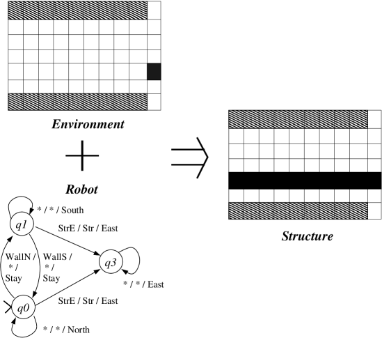
Figure 3: An example of distributed construction by a robot team (Adapted from Figures 1 and 2 in [16]). In the initial and final environments, wall and structure squares are indicated by hatching and black fill, respectively. The team consists of 9 copies of the pictured finite-state robot, which can only sense immediately-adjacent squares. Each transition is labeled with a triple $x/y/z$ where $x$ is the transition-activation formula, $y$ is the square-change (if any), and $z$ is the movement-action performed thereafter. See the main text for further details.

An example of a construction task performed by a team of 3-state FSR is shown in Figure 3. In this example, the initial environment consists of two parallel east-west-oriented walls of length $9$ and a structure seed square in the grid-column to the immediate east of two walls. The task is to construct an east-west oriented freespace-based linear structure (analogous to a painted lane-divider on a highway) extending westwards from the seed to the westmost edge of the environment. The initial position of the $9$ robots on the team is immediately to the north of the southern wall. The subsequent operation of the team creates the requested structure by “growing” it westwards from the initial seed, with the robots progressing eastwards along the seed-line into a holding area to the east (which for space reasons is not shown in the diagram). The required sensing of squares immediately around a robot can be implemented with robot sensory radius $r=1$ (under visual sensing) and scalar fields with source-value 1 and decay-value 0.5 (under scalar-field sensing). Note that this team operates correctly and deterministically as long as the seed square is not either immediately to the southeast of the north wall or immediately to the northeast of the south wall. Otherwise, the eastmost robot on the team will have two transitions enabled on first encountering the seed structure square to its immediate east (namely, $\{(q0,(\#,N),*,stay,q1),(q0,(X,E),(X,U),goNorth,q2)\}$ in the first case and $\{(q1,(\#,S),*,stay,q0),(q1,(X,E),(X,U),goSouth,q2)\}$ in the second case), which by the FSR operation rules discussed earlier will cause the team’s operation to terminate.

We can now formalize the computational problems that we will analyze in the remainder of this paper. Our problems relative to scalar-field environments and sensing are as follows:

Team / scalar-field environment verification (TeamEnvVerSF)
Input: An environment $E$ based on grid $G$ and field-set $S$, an FSR team $T$, a structure $X$, an initial positioning $p_{I}$ of $T$ in $E$, and a position $p_{X}$ of $X$ in $E$.
Question: Does $T$ started at $p_{I}$ in $E$ create $X$ at $p_{X}$?

Controller design by library selection (Scalar-field) (ContDesLSSF)
Input: An environment $E$ based on grid $G$ and field-set $S$, a requested team-size $|T|$, an initial positioning $p_{I}$ of $T$ in $E$, a structure $X$, a position $p_{X}$ of $X$ in $E$, a transition template library $L$, and positive integers $|Q|$ and $d$.
Output: An FSR controller $c$ with at most $|Q|$ states and at most $d$ transitions chosen from $L$ out of any state such that an FSR team with $|T|$ robots based on $c$ started at $p_{I}$ creates $X$ at $p_{X}$, if such a $c$ exists, and special symbol $\bot$ otherwise.

Team design by library selection (Scalar-field) (TeamDesLSSF)
Input: An environment $E$ based on grid $G$ and field-set $S$, a requested team-size $|T|$, an FSR library $L$, an initial region $E_{I}$ of size $T$ in $E$, a structure $X$, and a position $p_{X}$ of $X$ in $E$.
Output: An FSR team $T$ selected from $L$ such that $T$ started in $E_{I}$ creates $X$ at $p_{X}$, if such a a $T$ exists, and special symbol $\bot$ otherwise.

Scalar-field environment design (EnvDesSF)
Input: An environment-grid $G$, a field-set $S$, an FSR team $T$ based on controller $c$, a structure $X$, an initial positioning $p_{I}$ of $T$ in $G$, and a position $p_{X}$ of $X$ in $G$.
Output: An environment $E$ derived from $G$ and $S$ such that $T$ started at $p_{I}$ creates $X$ at $p_{X}$, if such an $E$ exists, and special symbol $\bot$ otherwise.

Team / scalar-field environment co-design by library selection
(TeamEnvDesLSSF)
Input: An environment-grid $G$, a field-set $S$, a team-size $|T|$, an FSR library $L$, a region $E_{I}$ of size $|T|$ in $G$, a structure $X$, and a position $p_{X}$ of $X$ in $G$.
Output: A team $T$ of size $|T|$ selected from $L$ and an environment $E$ derived from $G$ and $S$ such that $T$ started at $E_{I}$ in $E$ creates $X$ at $p_{X}$, if such a $T$ exists, and special symbol $\bot$ otherwise .

The above correspond to the following previously-analyzed problems that are relative to square-type environments and visual sensing:

Team / square-type environment verification (TeamEnvVerST)
Input: An environment $E$ based on square-type set $E_{T}$, a structure $X$, an initial positioning $p_{I}$ of $T$ in $E$, and a position $p_{X}$ of $X$ in $E$.
Question: Does $T$ started at $p_{I}$ in $E$ create $X$ at $p_{X}$?

Controller design by library selection (Square-type) (ContDesLSST)
Input: An environment $E$ based on square-type set $E_{T}$, a requested team-size $|T|$, an initial positioning $p_{I}$ of $T$ in $E$, a structure $X$, a position $p_{X}$ of $X$ in $E$, a transition template library $L$, and positive integers $r$, $|Q|$, and $d$.
Output: An FSR controller $c$ with sensory radius $r$, at most $|Q|$ states, and at most $d$ transitions chosen from $L$ out of any state such that an FSR team with $|T|$ robots based on $c$ started at $p_{I}$ creates $X$ at $p_{X}$, if such a $c$ exists, and special symbol $\bot$ otherwise.

Team design by library selection (Square-type) (TeamDesLSST)
Input: An environment $E$ based on square-type set $E_{T}$, a requested team-size $|T|$, an FSR library $L$, an initial region $E_{I}$ of size $T$ in $E$, a structure $X$, and a position $p_{X}$ of $X$ in $E$.
Output: An FSR team $T$ selected from $L$ such that $T$ started in $E_{I}$ creates $X$ at $p_{X}$, if such a a $T$ exists, and special symbol $\bot$ otherwise.

Square-type environment design (EnvDesST)
Input: An environment-grid $G$, a square-typed set $E_{T}$, an FSR team $T$ based on controller $c$, a structure $X$, an initial positioning $p_{I}$ of $T$ in $G$, and a position $p_{X}$ of $X$ in $G$.
Output: An environment $E$ derived from $G$ and $E_{T}$ such that $T$ started at $p_{I}$ creates $X$ at $p_{X}$, if such an $E$ exists, and special symbol $\bot$ otherwise.

Team / square-type environment co-design by library selection
(TeamEnvDesLSST)
Input: An environment-grid $G$, a square-type set $E_{T}$, a team-size $|T|$, an FSR library $L$, a region $E_{I}$ of size $|T|$ in $G$, a structure $X$, and a position $p_{X}$ of $X$ in $G$.
Output: A team $T$ of size $|T|$ selected from $L$ and an environment $E$ derived from $G$ and $E_{T}$ such that $T$ started at $E_{I}$ in $E$ creates $X$ at $p_{X}$, if such a $T$ exists, and special symbol $\bot$ otherwise .

Problems TeamDesLSSF and EnvDesSF are from [18], problems TeamEnvVerST, TeamDesLSST, EnvDesST, and TeamEnvDesST are the previously-analyzed problems ContEnvVer [16], DesCon [14], EnvDes [16], and CoDesignLS [12] and problem ContDesLSST is essentially problem ContDesLS [29] which was in turn a variation on previously-analyzed problem ContDes [16]. Without loss of generality, we will assume that each member of $T$ starts operating in the initial state $q_{0}$ of its associated controller. Following [14], we shall also assume for problems TeamDesLSST and TeamDesLSSF that (1) all FSR in $L$ are behaviorally distinct and (2) when tasks complete successfully, they do so relative to any positioning $p_{I}$ of the members of $T$ in $E_{I}$.

All of our problems above are simplifications of their associated real-world design problems. Many of these simplifications with respect to FSRs, FSR teams, and square-type environments have already been noted and discussed in [14, 16]. Our conception of scalar-field environments introduces additional simplifications (e.g., quantity-spread from a field source is instantaneous, decays as a linear function of Manhattan distance from the source, and is not affected by obstacles). The extent to which these simplifications affect the applicability of our results to real-world design problems in scalar-field environments can be addressed using arguments analogous to those presented previously in [14, 16] relative to visual sensing (see also Section 4.2). That being said, recall from Section 1 that our intent here is not so much to provide results of immediate use to real-world robots using visual and scalar-field sensors but rather to provide a simple setting in which to examine core computational characteristics of both types of sensing independent of conflating issues arising from errors in robot perception, control, and movement and more complex and realistic models of visual and scalar-field environments. This will be done in the next section.

3 Results

In this section, we first describe two types of efficient solvability, polynomial-time exact solvability and fixed-parameter tractability, and sketch the techniques by which unsolvability results are proven for these types (Section 3.1). Then, in Sections 3.2–3.6, we consider the five verification and design problems listed in Section 1. For each problem, we review previously obtained results for that problem relative to visual sensing in square-type environments as well as the techniques used to prove these results, and then describe what results and techniques carry over for that problem relative to scalar-field sensing and environments. To focus on the patterns in and implications of these results in the main text, all proofs of previously unpublished results are given in an appendix.

3.1 Types of Efficient Solvability

There are two basic questions when analyzing a problem $\Pi$ computationally: (1) is $\Pi$ efficiently solvable in general (i.e., for all possible inputs)?; and, if not, (2) under which restrictions (if any) is $\Pi$ efficiently solvable? These questions are based on the following two types of efficient solvability:

1. Polynomial-time exact solvability: An exact polynomial-time algorithm is a deterministic algorithm whose runtime is upper-bounded by $c_{1}|x|^{c_{2}}$, where $|x|$ is the size of the input $x$ and where $c_{1}$ and $c_{2}$ are constants, and is always guaranteed to produce the correct output for all inputs. A problem that has a polynomial-time algorithm is said to be polynomial-time tractable; otherwise, a problem that does not have such an algorithm is said to be polynomial-time intractable. Polynomial-time tractability is desirable because runtimes increase slowly as input size increases, and hence allow the solution of larger inputs.

2. Effectively polynomial-time exact restricted solvability: Even if a problem is not solvable in the sense above, a restricted version of that problem may be exactly solvable in close-to-polynomial time. Let us characterize restrictions on problem inputs in terms of a set $K=\{k_{1},k_{2},\ldots,k_{|K|}\}$ of aspects of the input. For example, possible restrictions on the inputs of ContDesLSSF could be the number of possible states and outgoing transitions per state in a controller and the number of transitions in the given transition template library (see also Table 1). Let $\langle K\rangle$-$\Pi$ denote a problem $\i$ so restricted relative to an aspect-set $K$.

   One of the most popular ways in which an algorithm can operate in close-to-polynomial time relative to restricted inputs is fixed-parameter (fp-) tractability [20]. Such an algorithm runs in time that is non-polynomial purely in terms of the aspects in $K$, i.e., in time $f(K)|x|^{c}$ where $f()$ is some function, $|x|$ is the size of input $x$, and $c$ is a constant. A problem with such an algorithm for aspect-set $K$ is said to be fixed-parameter (fp-)tractable relative to $K$. Fixed-parameter tractability generalize polynomial-time exact solvability by allowing the leading constant $c_{1}$ of the input size in the runtime upper-bound of an algorithm to be a function of $K$. Though such algorithms run in non-polynomial time in general, for inputs in which all the aspects in $K$ have very small constant values and $f(K)$ thus collapses to a possibly large but nonetheless constant value, such algorithms (particularly if $f()$ is suitably well-behaved, (e.g, $(1.2)^{k_{1}+k_{2}}$) may be acceptable.

The second type is useful in isolating and investigating sources of computational intractability in problems. Following [33], for a set of aspects $K$ of a problem $\Pi$, we say that $K$ is a source of intractability in $\Pi$ if $\langle K\rangle$-$\Pi$ is fp-tractable; if $K$ is such that $\langle K^{\prime}\rangle$-$\Pi$ is not fp-tractable for any subset $K^{\prime}\subset K$, then this source of computational intractability is also minimal. Such sources of intractability (particularly if they are minimal) are very useful in highlighting those mechanisms in a problem that interact and can (if allowed to operate in an unrestricted manner) yield intractability (Section 4.1).

Table 1: Parameters for Design Problems in Square-type (ST) and Scalar-field (SF) Environments. These parameters are divided into four groups: (1) parameters characterizing robot teams ($|T|$, $h$); (2) parameters characterizing individual robots ($|Q|$, $d$, $|f|$, $r$,); (3) parameters characterizing the controller and team design process ($|L|$); and (4) parameters charactering environments and requested structures ($|E|$, $|E_{T}|$, $|S|$, $|S_{E}|$, $|q_{E}|$, $|X|$). The problems to which each parameter is applicable are indicated in the third column of the table.

Parameter	Description	Applicability
$|T|$	# robots in team	All
$h$	# robot-types in team	All
$|Q|$	Max # states per robot	All
$d$	Max # outgoing transitions per state	All
$|f|$	Max length transition-trigger formula	All
$r$	Sensory radius of robot	ST only
$|L|$	# entities in design library	ContDesLSS*,
		TeamDesLSS*,
		TeamEnvDesLSS*
$|E|$	# squares in environment	All
$|E_{T}|$	# environment square-types	ST only
$|S|$	# scalar-field types	SF only
$|S_{E}|$	Max # scalar-fields in environment	SF only
$|q_{E}|$	Max # scalar-fields of type $q$ in environment	SF only
$|X|$	# squares in structure	All

To show solvability of a problem $\Pi$ relative to one of the above types, one need only give an algorithm of that type for $\Pi$. To show unsolvability, we use reductions between pairs of problems, where a reduction from a problem $\Pi$ to a problem $\Pi^{\prime}$ is essentially an efficient algorithm $A$ for solving $\Pi$ which uses a hypothetical algorithm for solving $\Pi^{\prime}$. Reductions are useful in two ways:

1. If $\Pi$ reduces to $\Pi^{\prime}$ and $\Pi^{\prime}$ is efficiently solvable by algorithm $B$ then $\Pi$ is efficiently solvable (courtesy of the algorithm $A^{\prime}$ that invokes $A$ relative to $B$).

2. If $\Pi$ reduces to $\Pi^{\prime}$ and $\Pi$ is not efficiently solvable then $\Pi^{\prime}$ is not efficiently solvable (as otherwise, by the logic of (1) above, $\Pi$ would be efficiently solvable, which would be a contradiction).

Each of our types of efficient solvability has its own associated type of reducibility designed to pass that type of solvability backwards along a reduction by the logic of (1) above. These are the standard reducibilities for polynomial-time exact and fixed-parameter solvability.

Definition 1

[34, Section 3.1.2] Given decision problems $\Pi$ and $\Pi^{\prime}$, i.e., problems whose answers are either “Yes” or “No”, $\Pi$ polynomial-time (Karp) reduces to $\Pi^{\prime}$ if there is a polynomial-time computable function $f()$ such that for any instance $x$ of $\Pi$, the answer to $\Pi$ for $x$ is “Yes” if and only if the answer to $\Pi^{\prime}$ for $f(x)$ is “Yes”.

Definition 2

[20] Given parameterized decision problems $\Pi$ and $\Pi^{\prime}$, $\Pi$ parameterized reduces to $\Pi^{\prime}$ if there is a function $f()$ which transforms instances $\langle x,K\rangle$ of $\Pi$ into instances $\langle x^{\prime},K^{\prime}\rangle$ of $\Pi^{\prime}$ such that $f()$ runs in $f^{\prime}(K)|x|^{c}$ time for some function $f^{\prime}()$ and constant $c$, $k^{\prime}=g_{k^{\prime}}(K)$ for each $k^{\prime}\in K$ for some function $g_{k^{\prime}}()$, and for any instance $\langle x,K\rangle$ of $\Pi$, the answer to $\Pi$ for $\langle x,K\rangle$ is “Yes” if and only if the answer to $\Pi^{\prime}$ for $f(\langle x,K\rangle)$ is “Yes”.

For technical reasons, our reducibilities operate on and establish unsolvability of decision problems. Of the problems defined in Section 2, only TeamEnvVerSF and TeamEnvVerST are currently decision problems. However, this is not an issue if decision versions of the other non-decision problems are formulated such that they can be solved efficiently using algorithms for those non-decision problems, as such algorithms allow unsolvability results for the decision problems to propagate to their associated non-decision problems (see the appendix for details).

Our reductions will be from the following decision problems:

Compact Deterministic Turing Machine computation (CDTMC)
[19, Problem AL3]
Input: A deterministic Turing Machine $M$ with state-set $Q$, tape alphabet $\Sigma$, and transition-function $\delta$, an input $x$, and a positive integer $k$.
Question: Does $M$ accept $x$ in a computation that uses at most $k$ tape squares?

Dominating set [19, Problem GT2]
Input: An undirected graph $G=(V,E)$ and a positive integer $k$.
Question: Does $G$ contain a dominating set of size $k$, i.e., is there a subset $V^{\prime}\subseteq V$, $|V^{\prime}|=k$, such that for all $v\in V$, either $v\in V^{\prime}$ or there is at least one $v^{\prime}\in V^{\prime}$ such that $(v,v^{\prime})\in E$?

3-Satisfiability (3SAT) [19, Problem LO2]
Input: A set $U$ of variables and a set $C$ of disjunctive clauses over $U$ such that each clause $c\in C$ has $|c|=3$.
Question: Is there a satisfying truth assignment for $C$?

Clique [19, Problem GT19]
Input: An undirected graph $G=(V,E)$ and a positive integer $k$.
Question: Does $G$ contain a clique of size $k$, i.e., is there a subset $V^{\prime}\subseteq V$, $|V^{\prime}|=k$, such that for all $u,v\in V^{\prime}$, $(u,v)\in E$?

In addition to the four problems above, we shall also make use of Dominating set^PD3, the version of Dominating set in which the given graph $G$ is planar and each vertex in $G$ has degree at most 3. For each vertex $v\in V$ in a graph $G$, let the complete neighbourhood $N_{C}(v)$ of $v$ be the set composed of $v$ and the set of all vertices in $G$ that are adjacent to $v$ by a single edge, i.e., $v\cup\{u~{}|~{}u~{}\in V~{}\rm{and}~{}(u,v)\in E\}$. We assume below for each instance of Clique and Dominating set an arbitrary ordering on the vertices of $V$ such that $V=\{v_{1},v_{2},\ldots,v_{|V|}\}$. Versions of these problems are only known to be tractably unsolvable modulo the conjectures $P\neq NP$ and $FPT\neq W[1]$; however, this is not a problem in practice as both of these conjectures are widely believed within computer science to be true [36, 37].

There are a variety of techniques for creating reductions from a problem $\Pi$ to a problem $\Pi^{\prime}$ (Section 3.2 of [19]; see also Chapters 3 and 6 of [35]). One of these techniques, component design (in which a constructed instance of $\Pi^{\prime}$ is structured as components that generate candidate solutions for the given instance of $\Pi$ and check these candidates to see if any are actual solutions), will be used extensively in the following subsections. Creating such reductions can be difficult. However, with a bit of forethought, a single reduction can often be constructed such that it yields multiple results. For example, as algorithms that run in polynomial time also run in fixed-parameter tractable time, provided the appropriate relationships specified by the functions $g_{k^{\prime}}()$ in Definition 2 hold between parameters of interest, a polynomial-time reduction can imply both polynomial-time exact and fixed-parameter intractability results. Moreover, given a fp-tractability or intractability result, additional fp-tractability and intractability results can often be derived using the following easily-proven lemmas.

Lemma 1

[38, Lemma 2.1.30] If problem $\Pi$ is fp-tractable relative to parameter-set $K$ then $\Pi$ is fp-tractable for any parameter-set $K^{\prime}$ such that $K\subset K^{\prime}$.

Lemma 2

[38, Lemma 2.1.31] If problem $\Pi$ is fp-intractable relative to parameter-set $K$ then $\Pi$ is fp-intractable for any parameter-set $K^{\prime}$ such that $K^{\prime}\subset K$.

As we shall see later in this paper, these lemmas are of use use both in establishing the minimality of sources of intractability and in more easily establishing the parameterized complexity of a problem relative to all combinations of parameters in a given parameter-set, i.e., performing a systematic parameterized complexity analysis [38] .

In the following subsections, we shall, in addition to our tractability and intractability results, discuss the algorithms and reductions by which we derive these results. To highlight such details is admittedly unusual outside of the theoretical computer science literature. However, we believe that even a basic appreciation of the ways in which a problem’s mechanisms interact in algorithms to yield tractability and in reductions to yield intractability can give useful insights into that problem, with the latter also providing ready targets for subsequent restrictions that may yield additional efficient algorithms.

3.2 Team / Environment Verification

In a team / environment verification problem, both the robot team and the environment are given as part of the problem input, so there is no opportunity to use an unspecified part of the constructed instance of that problem in a candidate-solution generation component for the given instance of $\Pi$ in a reduction from $\Pi$ to that problem. Rather, the operation of the given robot team in its given environment must be structured to effectively simulate the mechanisms in $\Pi$ itself. Such is the case in the following result for TeamEnvVerST.

Result A.ST.1

[16, Result A]: TeamEnvVerST is not polynomial-time exact solvable.

This result was proved by a polynomial-time reduction from CDTMC to TeamEnvVerST, in which an instance of TeamEnvVerST is constructed such that the environment $E$ corresponds to the DTM tape, the square-types in $E_{T}$ correspond to the tape alphabet $\Sigma$, and the single robot in $T$ corresponds to the DTM $M$’s deterministic controller and tape read/write head. The operation of this robot in $E$ thus effectively simulates the computation of $M$ on $x$.

A most useful aspect of this reduction is that as the TM read/write head only views a single tape-square at a time, the robot in $T$ has sensory radius $r=0$. Given this, we can easily modify the reduction sketched above to show the polynomial-time intractability of TeamEnvVerSF — as $r=0$, we can simulate the tape-squares in $E_{T}$ using point-fields with source-value and decay 1 (i.e., the field-quantity in each such point-field is only detectable in the square at which the point-field is positioned) and thus trivially modify the visual sensing robot to create an equivalent scalar-field sensing robot. This yields the following result.

Result A.SF.1:

TeamEnvVerSF is not polynomial-time exact solvable.

Given this, we will restrict our four scalar-field design problems to operate in polynomial time; this is denoted adding the superscript $fast$ to the problem name, e.g., ContDesLSSF^fast. This notion of time-bounded robot team operation, introduced in [16] as $(c_{1},c_{2})$-completability. requires that each robot team complete its task within $c_{1}|E|^{c_{2}}$ timesteps for constants $c_{1}$ and $c_{2}$. We here make two modifications to this notion. First, as was done in [12], we broaden the timestep bound to $c_{1}(|E|+|Q|)^{c_{2}}$ to accommodate FSR that make a number of internal state-changes without moving. Second, as was done in [39], $c_{1}$ and $c_{2}$ are no longer part of problem inputs but are rather fixed beforehand, which allows us to avoid certain technical issues. To ensure generous but nonetheless low-order polynomial runtime bounds, we will assume that $c_{1}=10$ and $c_{2}=3$.

The above demonstrates that even though scalar-field sensing seems simpler than visual sensing, it still has the same degree of computational intractability when it comes to controller / environment verification. Moreover, we have also seen that the two types of sensing are equivalent (in the sense that robots with one type of sensing can simulate robots with the other type) when $|T|=1$ and $r=0$ given appropriately restricted point fields. That being said, as we shall see in the following subsections, this equivalence most decidedly does not hold in general.

3.3 Controller Design by Library Selection

Unlike the team / environment verification problems examined in Section 3.2, a controller design by library selection problem gives the general form but not the exact structure of the robot controller as part of the problem input. Hence, the transition-template library $L$ and the values of $|Q|$ and $d$ can be specified to create a candidate-solution generation component and the environment can be specified to serve as a candidate-solution checking component for the given instance of $\Pi$ in a reduction from $\Pi$ to our controller design by library selection problem.

Such is the case in previous results for controller design that were proved relative to a problem ContDes^fast [16], in which controller transitions were designed from scratch by including $|f|$ as part of the problem input. The polynomial-time exact intractability result for this problem [16, Result B] used a reduction from Dominating set to create a somewhat complex environment for a team composed of a single-state robot (see Figure 4(b)). In order to force the transitions in such a robot to encode a candidate dominating set of size $k$ in the given graph $G$, the robot had to navigate from the southwestmost corner of the environment to the top of the $(k+1)$st column in subgrid SG1 (see Figure 4(c)). From there, the robot navigated the $|V|$ columns of subgrid SG2 (see Figure 4(d)), where each column represented the vertex neighbourhood of a particular vertex in $G$ and the robot could progress eastward from one column to the next if and only if that robot had a transition corresponding to a vertex in the neighbourhood encoded in the first column. Subgrid SG2 thus checked if the robot encoded an actual dominating set of size $k$ in $G$, such that the robot could enter the northeastmost square of the environment and build the requested structure there if and only if the $k$ east-moving transitions in the robot encoded a dominating set of size $k$ in $G$.

Figure 4: A sample graph and its associated team-environment (Modified from Figure 2 in [17]). a) An undirected graph on five vertices. b) The general structure of the team-environment $E$ constructed by the reduction in the proof of Result B in [16] from a given instance $(G=(V,E),k)$ of Dominating set. Note that this environment is not drawn to scale but rather to illustrate the large-scale features of the environment. c) The subgrid SG1 constructed from the graph in part (a) when $k=3$. d) The column-fragments of the subgrid SG2 constructed from the graph in part (a) that correspond to the vertex-neighborhoods of the vertices in that graph.

By using an appropriate transition template library $L$, we can simplify the reduction sketched above as in [29] such that we no longer need the northwest $e_{N}$-based or SG1 subgrids in the environment or the restriction on $|f|$ in the problem input. This yields the following result.

Result B.ST.1 (Modified from [29, Result B]):

ContDesLSST^fast is not polynomial-time exact solvable.

As $|T|=1$ and $r=0$ in this reduction, we can easily employ the techniques sketched in the previous subsection to derive our next result.

Result B.SF.1:

ContDesLSSF^fast is not polynomial-time exact solvable.

Given the above, it is natural to wonder under which restrictions efficient solvability is possible. Let us first consider fixed-parameter intractability results, starting with problem ContDesLSST^fast. Our first result follows directly from the reduction by which we proved polynomial-time intractability.

Result B.ST.2:

$\langle|T|,h,|Q|,d,|f|,r,|X|\rangle$-ContDesLSST^fast is fp-intractable.

We can in turn restrict $E_{T}$ at the cost of unrestricted $r$ by replacing each occurrence of a vertex-symbol in a column of the environment with a $(|V|+1)$-length row, in which the eastmost marker-symbol in the row indicates that a vertex is present in that column’s neighbourhood and the position of a vertex-symbol in one of the first $|V|$ squares indicates which vertex it is (see Figure 5(a)).

Figure 5: Reducing the number of square-types and scalar-field types in complex environments. a) Replacing multiple vertex-symbols with pairs of vertex- and marker-symbols (see main text and proof of Result B.ST.3 for details). This is done relative to a vertex-neighbourhood containing $v_{1}$ and $v_{2}$ when $|V|=4$. b) Interference problems with respect to field-quantity $fq_{V}$ created by straightforward replacement of vertex- and marker-symbols with vertex and marker point-fields (vertex-neighborhood and vertices as in (a)). Note that courtesy of interference, both of these vertices in these rows would be misperceived as non-existent vertex $v_{6}$ at the marker-field positions. c) Proper replacement of vertex- and marker-symbols with vertex and marker point-fields under appropriate row-separation (i.e., $2|V|$ separating rows) to avoid interference (vertex-neighbourhood and vertices as in (a)) (see main text and proof of Result B.SF.4 for details). Vertex and marker positions in all subfigures are indicated by boldfaced boxes.

Result B.ST.3:

$\langle|T|,h,|Q|,d,|f|,|E_{T}|,|X|\rangle$-ContDesLSST^fast is fp-intractable.

Result B.ST.2 also holds for problem ContDesLSSF^fast courtesy of the reduction in the proof of Result B.SF.1. Moreover, if we in turn modify that reduction to reduce from Dominating set^PD3 (in which each vertex appears in at most four vertex neighborhoods, those of its three neighbors and its own) instead of Dominating set, we get a second result for free.

Result B.SF.2:

$\langle|T|,h,|Q|,d,|f|,|X|\rangle$-ContDesLSSF^fast is fp-intractable.

Result B.SF.3:

$\langle|T|,h,|Q|,|f|,|q_{E}|,|X|\rangle$-ContDesLSSF^fast is fp-intractable.

The second of our fp-intractability results for ContDesLSST^fast, however, does not translate over so directly. This is because, for the first time, we must use point-fields whose influence propagates beyond the square in which they are placed — indeed, to encode the vertex-symbols, we need a corresponding vertex point-field that is detectable up to $|V|$ squares from its source (Figure 2(c)). Straightforward implementations of such point-fields in adjacent rows of the environment can interfere to destroy the encodings of vertices associated with these point-fields (Figure 5(b)). This interference can be mitigated by increasing the separations between the rows in which vertex point-fields occur so that these point-fields do not interfere at all (see Figure 5(c)), at the cost of increasing the size of the resulting environment.

Result B.SF.4:

$\langle|T|,h,|Q|,d,|f|,|S|,|X|\rangle$-ContDesLSSF^fast is fp-intractable.

Let us now consider fixed-parameter tractability. In this case, we once again have equivalence of results because the proofs of these results rely only on the combinatorics of combining states and transitions from transition template library $L$ to create controllers, and these combinatorics are identical for problems ContDesLSST^fast and ContDesLSSF^fast.

Result B.ST.4:

$\langle|Q|,|L|\rangle$-ContDesLSST^fast is fp-tractable.

Result B.SF.5:

$\langle|Q|,|L|\rangle$-ContDesLSSF^fast is fp-tractable.

Note that both of these results collapse to fp-tractability relative to $|L|$ alone when $|Q|=1$.

A summary of all of our fixed-parameter results derived in this subsection is given in Table 2. Given our fp-intractability results at this time, neither of our fp-tractability results are minimal in the sense described in Section 3.1.

Table 2: A Detailed Summary of Our Fixed-parameter Results for Controller Design by Library Selection. Each column in this table is a result which holds relative to the parameter-set consisting of all parameters with a @-symbol in that column. If the result holds when a particular parameter has a constant value $c$, that is indicated by $c$ replacing @ for that parameter in that result’s column. Note that within each result-group, intractability results are first and tractability results (shown in bold) are last.

	Square-type (ST)			Scalar-field (SF)
	ST.2	ST.3	ST.4	SF.2	SF.3	SF.4	SF.5
$|T|$	1	1	–	1	1	1	–
$h$	1	1	–	1	1	1	–
$|Q|$	1	1	@	1	1	1	@
$d$	@	@	–	@	–	@	–
$|f|$	1	3	–	1	1	3	–
$r$	0	–	–	N/A	N/A	N/A	N/A
$|L|$	–	–	@	–	–	–	@
$|E|$	–	–	–	–	–	–	–
$|E_{T}|$	–	5	–	N/A	N/A	N/A	N/A
$|S|$	N/A	N/A	–	–	–	5	–
$|S_{E}|$	N/A	N/A	–	–	–	–	–
$|q_{E}|$	N/A	N/A	–	–	4	–	–
$|X|$	1	1	–	1	1	1	–

The above demonstrates that results derived by utilizing perception at a distance relative to visual sensing (i.e., $r>0$) can still hold relative scalar-field sensing; however, this comes at the cost of larger environments to avoid interference between separate fields based on the same field-quantity. This problem with interference will re-occur in many of the results described in the following subsections.

3.4 Team Design by Library Selection

Team design by library selection is unique among the design problems considered in this paper, in that it is the only one that is currently known to have a restricted case that is solvable in polynomial time — namely, for homogeneous robot teams whose members all have the same controller, i.e., $h=1$.

Result C.ST.1

[14, Result A]: TeamDesLSST^fast is polynomial-time exact solvable when $h=1$.

This does not, however, hold when teams are heterogeneous, i.e., $h>1$.

Result C.ST.2

[14, Result B]: TeamDesLSST^fast is not exact polynomial-time solvable when $h>1$.

The reduction underlying this result exploits the fact that the general form but not the exact structure (in terms of individual member FSRs) of the team is given as part of the problem input. Hence, analogous to the case with controller design by library selection in Section 3.3, the FSR library $L$ and the value of $|T|$ can be specified to create a candidate-solution generation component and the environment can be specified to serve as a candidate-solution checking component for the given instance of a suitable problem, which is once again Dominating set.

The reduction works as follows [14]: for a given instance of Dominating set, we construct an environment like that in part (a) of Figure 1 such that a team of $k+1$ robots will be able to co-operatively construct a single-square structure at the square with type $e_{T}$ if and only if there is a dominating set of size at most $k$ in the graph in the given instance of Dominating set. The robots are initially positioned in the top-left corner of the movement-track and move in a counter-clockwise fashion around this track. A functional robot team of $|T|=k+1$ robots, each with sensory radius $r=1$, selected from $L$ consists of at most $k$ “vertex neighbourhood” robots which attempt to fill in a scaffolding of squares in the center of the central line of squares and at least one “checker” robot which determines if all squares in this scaffolding are eventually filled in (which only occurs if the vertex-neighborhood robots encode a dominating set of size at most $k$ in $G$) and, if so, places the single square corresponding to the requested structure at the square with type $e_{T}$. Note that as the two types of robots in this reduction only communicate indirectly via additions to and the sensing of the central scaffolding, this is a good example of communication by stigmergy [32].

The reduction above in turn yields three fixed-parameter intractability results. The first of these follows directly from this reduction, and the second by modifying this reduction to collapse a set of short-triggering-formula transitions between a pair of states into a single long-triggering-formula transition between those states.

Result C.ST.3

[14, Result E]: $\langle|T|,h,|Q|,|f|,r,|X|\rangle$-TeamDesLSST^fast is fp-intractable.

Result C.ST.4:

$\langle|T|,h,|Q|,d,r,|X|\rangle$-TeamDesLSST^fast is fp-intractable.

The third of our fp-intractability results for TeamDesLSST^fast makes two modifications to the reduction in the proof of Result C.ST.2. First, each of the vertex-symbols $e_{Vi}$ in the southmost row of $E$ is replaced with a column of height $\lceil\log_{2}|V|\rceil$ giving a binary encoding of $i$ using symbols $e_{0}$ and $e_{1}$; as such, this is an alternate scheme to that based on vertex- and marker-symbols used in the proof of Result B.ST.3 for restricting $|E_{T}|$. Second, the tradeoff between transition trigger-formula length and number of outgoing transitions per state described above is applied.

Result C.ST.5:

$\langle|T|,h,|Q|,d,|E_{T}|,|X|\rangle$-TeamDesLSST^fast is fp-intractable.

We also have the following fp-tractability results.

Result C.ST.6

[14, Result G]: $\langle|T|,|L|\rangle$-TeamDesLSST^fast is fp-tractable.

Result C.ST.7

[14, Result I]: $\langle|T|,|Q|,r,|E_{T}|\rangle$-TeamDesLSST^fast is fp-tractable.

The first result is analogous to that in Result B.ST.4, in that it relies only on the combinatorics of making $|T|$ choices from $L$ to make teams. The second result in turns modifies the first by using combinatorics based on $|Q|$, $r$, and $|E_{T}|$ to bound the number of possible behaviorally-distinct FSRs in $L$.

Let us now consider to what extent the results above for TeamDesLSST^fast transfer over to TeamDesLSSF^fast. As the algorithm underlying Result C.ST.1 relies only on the timestep-bound on successful team task completion imposed by $(c_{1},c_{2})$ completability, the same result holds for TeamDesLSSF^fast.

Result C.SF.1

[18, Result A.1]: TeamDesLSSF^fast is exact polynomial-time solvable when $h=1$.

An analogue of the polynomial-time exact intractability in Result C.ST.2 when teams are heterogeneous also holds.

Result C.SF.2

[18, Result A.2] TeamDesLSSF^fast is not exact polynomial-time solvable when $h>1$.

There are, however, complications due to point-field interference. Oddly enough, this is not due to environmental point-fields. As $r=1$ in the reduction above, given the structure of the environment shown in Figure 1(a), all squares in both the outer ring and the central scaffolding can readily have their symbols replaced with corresponding point-fields with source-value 1 and decay 0.5. Provided appropriate care is taken (see Figure 2(d)), no robot traveling around the movement-track will ever misperceive any field-quantity related to those squares.

The problem this time (summarized succinctly in Figure 6) is interference generated by the point-fields associated with the robots themselves. The visual sensing robots in the reduction in the proof of Result C.ST.2 need only ensure that there is no robot in a square they want to move into to safely move into that square. Scalar-field sensing robots cannot do this — indeed, as we cannot be sure what other robots are nearby and in what positions, Figure 6 shows that it is difficult even on a linear movement-track for a scalar-field sensing robot to determine whether or not there is a robot already in a square to which it wishes to move. Figures 6(e)-(h) suggest that when $fval(fq_{robot},\leq,1.5)$ is $True$, legal movement to be possible. However, this alone is not sufficient as it would allow illegal movement in the situations shown in Figures 6(c) and (d). We can add a gradient-sensing predicate in the direction $dir$ in which movement is wanted, but there are again problems. If we use $fgrd(fq_{robot},\geq,dir)$, we allow not only the legal movement in Figures 6(e)-(h) but also the illegal movement in Figures 6(b) and (c); on the other hand, if we use use $fgrd(fq_{robot},>,dir)$, we disallow the illegal movement in Figures 6(b) and (c) at the cost of also disallowing the legal movement in Figure 6(h). There does not seem to be a perfect solution. Hence, we here adopt the second alternative, consoling ourselves with the thought that, as the environments constructed in our reduction are big enough that there will always be at least one pair of robots separated by two or more spaces on the movement track, any situation like that shown in Figure 6(h) eventually becomes one of the situations in Figures 6(e) or (g) that are covered by our adopted solution.

Figure 6: Scalar-field sensing of adjacent robots on a linear movement-track (Figure 2 in [18]). This figure shows the eight possible situations when a scalar-field sensing robot on a linear movement-track (indicated by the bold-faced rounded square) is trying to determine if there is already another robot in a square which it is considering moving into. Subfigures (a)-(d) and (e)-(h) depict situations in which movement is illegal and legal, respectively. For simplicity, we only show the case of eastward movement, though movement in all other directions are analogous. We also collapse movement in the middle of tracks and into corners as these too are analogous; the rightmost square in each situation is thus either on the same line as the others squares or one above the third square. In each situation, we show the values of field-quantity $fq_{robot}$ in both the square currently occupied by the robot and the square which that robot is considering moving into.

The reduction above in turn yields several fixed-parameter intractability results. The first pair of fp-intractability results follows directly from this reduction, with the second result in the pair using the tradeoff between transition trigger formula length and number of transitions per state sketched for Result C.ST.4.

Result C.SF.3

[18, Result A.3]: $\langle|T|,h,|Q|,|f|,|X|\rangle$-TeamDesLSST^fast is fp-intractable.

Result C.SF.4

[18, Result A.4]: $\langle|T|,h,|Q|,d,|X|\rangle$-TeamDesLSST^fast is fp-intractable.

The second pair of fp-intractability results modifies the reduction in the proof of Result C.SF.2 along the lines in the proof of Result B.SF.4 to both (1) replace each of the vertex point-fields $s_{Vi}$ in the lower row with a column of height $|V|+1$ and appropriately-positioned vertex and marker point-fields and (2) place $2|V|$ blank columns between each pair of vertex-columns to prevent vertex point-field interference. Once again, the second result in the pair uses the tradeoff between transition trigger formula length and number of transitions per state sketched above.

Result C.SF.5

[18, Result A.5]: $\langle|T|,h,|Q|,|f|,|S|,|X|\rangle$-TeamDesLSST^fast is fp-intractable.

Result C.SF.6

[18, Result A.6]: $\langle|T|,h,|Q|,d,|S|,|X|\rangle$-TeamDesLSST^fast is fp-intractable.

We also have the following fixed-parameter tractability result.

Result C.SF.7

[18, Result A.7]: $\langle|T|,|L|\rangle$-TeamDesLSST^fast is fp-tractable.

This result follows directly from the algorithm in the proof of Result C.ST.6. Unfortunately, we do not have an analogue for TeamDesLSSF^fast of Result C.ST.7 as there does not appear to be a way to combinatorially bound the number of possible behaviorally-distinct scalar-field sensing FSR using the problem-aspects in Table 1.

A summary of all of our fixed-parameter results derived in this subsection is given in Table 3. Given our fp-intractability results at this time, none of our fp-tractability results are minimal in the sense described in Section 3.1.

The above demonstrates that problems with point-field interference can occur with even the simplest non-trivial point-fields that are perceptible out to only Manhattan distance one from the point-field source if point-fields are dynamic (i.e., associated with robots) rather than static (i.e., associated with the environment). Nonetheless, these problems are resolvable. As we shall see in the next section, they are also resolvable (at the cost of more complex robots and environments, including our first use of edge-fields) in cases involving perception at Manhattan distances arbitrarily larger than one.

Table 3: A Detailed Summary of Our Fixed-parameter Results for Team Design by Library Selection. This table is interpreted as described in the caption of Table 2.

	Square-type (ST)					Scalar-field (SF)
	ST.3	ST.4	ST.5	ST.6	ST.7	SF.3	SF.4	ST.5	ST.6	SF.7
$|T|$	@	@	@	@	@	@	@	@	@	@
$h$	@	@	@	–	–	@	@	@	@	–
$|Q|$	3	3	3	–	@	3	3	3	3	–
$d$	–	7	7	–	–	–	7	–	7	–
$|f|$	16	–	–	–	–	27	–	31	–	–
$r$	1	1	–	–	@	N/A	N/A	N/A	N/A	N/A
$|L|$	–	–	–	@	–	–	–	–	–	@
$|E|$	–	–	–	–	–	–	–	–	–	–
$|E_{T}|$	–	–	13	–	@	N/A	N/A	N/A	N/A	N/A
$|S|$	N/A	N/A	N/A	N/A	N/A	–	–	13	13	–
$|S_{E}|$	N/A	N/A	N/A	N/A	N/A	–	–	–	–	–
$|q_{E}|$	N/A	N/A	N/A	N/A	N/A	–	–	–	–	–
$|X|$	1	1	1	–	–	1	1	1	1	–

3.5 Environment Design

Unlike all problems examined so far in this paper, an environment design problem gives the general form but not the exact structure of the environment as part of the problem input. Hence, the environment size $|E|$ and the environment-square contents (either square-type set $E_{T}$ or field-set $S$ in the case of EnvDesST^fast or EnvDesSF^fast, respectively) can be specified to create a candidate-solution generation component and the robot team $T$ can be specified to serve as a candidate-solution checking component for the given instance of $\Pi$ in a reduction from $\Pi$ to our environment design problem.

This was done in [16] for EnvDesST^fast using reductions from 3SAT and Clique in which the environment had the two-column structure shown in Figure 7(a). In the reductions from 3SAT, the candidate solution to the given instance of 3SAT was encoded in the northmost $|V|$ squares of the first column and the sole robot in $T$ was in the southmost square of that column. If this robot determined that the candidate solution so encoded was an actual solution to the given instance of 3SAT, the robot moved one square to the east and created the requested structure $X$ in the southmost square of the second column. This yielded the following result.

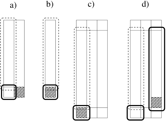
Figure 7: General structures of environments used to encode candidate solutions in environment design problems (Modified from Figure 3 in [18]). a) Environment structure for reductions to EnvDesST^fast. b) Environment structure for reductions to EnvDesSF^fast involving single-robot teams (Results D.SF.1–D.SF.3). c) Environment structure for reductions to EnvDesSF^fast involving single-robot teams (Results D.SF.4 and D.SF.5). d) Environment structure for reduction to EnvDesSF^fast involving multi-robot teams (Results D.SF.6). In each environment, the region encoding the candidate solution is indicated by a dashed box, the initial positioning of the robots is indicated by boldface boxes, and the position of the requested structure is indicated by a cross-hatched box.

Result D.ST.1

[16, Result C]: EnvDesST^fast is not exact polynomial-time solvable.

This reduction in turn gave the first two parameterized intractability results, the second of these by modifying the reduction to apply the tradeoff between transition trigger-formula length and the number of outgoing transitions per state sketched in Section 3.4.

Result D.ST.2

[16, Result H]: $\langle|T|,|f|,d,|E_{T}|,|X|\rangle$-EnvDesST^fast is fp-intractable.

Result D.ST.3

[16, Result I]: $\langle|T|,|Q|,d,|E_{T}|,|X|\rangle$-EnvDesST^fast is fp-intractable.

The remaining two previous parameterized intractability results instead used a reduction from Clique in which the northmost $k$ squares in the first column encoded the vertices in a candidate clique of size $k$. The number of states in the single checking robot was also bounded by a function of $k$ as the number of states required to implement the required solution-checks ($k$ states to verify that the vertices in the encoded candidate solution are all different and $k(k-1)/2$ states to verify that there is an edge between each pair of vertices in the candidate solution in the graph $G$ in the given instance of Clique) was also a function of $k$.

Result D.ST.4

[16, Result J]: $\langle|T|,|Q|,|f|,r,|E|,|X|\rangle$-EnvDesST^fast is fp-intractable.

Result D.ST.5

[16, Result K]: $\langle|T|,|Q|,d,r,|E|,|X|\rangle$-EnvDesST^fast is fp-intractable.

The second of these results used the tradeoff between transition trigger-formula length and number of outgoing transitions per state sketched above. There was a single previous parameterized tractability result,

Result D.ST.6

[16, Result N]: $\langle|E|,|E_{T}|\rangle$-EnvDesST^fast is fp-tractable.

This result was based on the brute-force enumeration of all possible environments and checking of robot team operation in each of those environments.

The intractability results above do not translate over to problem EnvDesSF^fast. This is because the complex sensing at a distance between pairs of elements in the candidate solution encoded in $E$ required by a reduction from Clique is impossible to implement with scalar-field sensing. That being said, the scalar-field sensing at a distance illustrated in Figure 2(c) can work for a reduction from Dominating set using an environment such as that in Figure 7(b). By using different point-fields for each vertex in given graph $G$, a suitably configured scalar-field sensing robot positioned at the southmost end of the single column in the environment can step through a set of single-element checks to see if the encoded candidate solution contains at least one vertex in each vertex neighborhood in given graph $G$. The size of the environment ensures that there are at most $k$ vertices in the candidate solution, and we don’t care if the same element occurs multiple times as (1) this will not interfere with the detection of that element by the robot (i.e., we only care about the presence and not the position of an element) and (2) we are interested in the presence in $G$ of dominating sets with at most and not necessarily exactly $k$ vertices. This reduction yields the following initial result.

Result D.SF.1

[18, Result B.1]: EnvDesSF^fast is not polynomial-time exact solvable.

It also yields our first pair of fixed-parameter intractability results, with the second in the pair using the tradeoff between transition trigger-formula length and number of outgoing transitions per state sketched above.

Result D.SF.2

[18, Result B.2]: $\langle|T|,h,|f|,|E|,|S_{E}|,|q_{E}|,|X|\rangle$-EnvDesSF^fast is fp-intractable.

Result D.SF.3

[18, Result B.3]: $\langle|T|,h,|Q|,d,|E|,|S_{E}|,|q_{E}|,|X|\rangle$-EnvDesSF^fast is fp-intractable.

The sensing at a distance approach sketched above will not work if we want to restrict the number of types of point-fields in $S$, as a static checker-robot cannot verify the positions of sensed point-fields encoding only the presence of vertices in a column of $|V|$ squares. However, taking our cue from the dynamic robots in Sections 3.3 and 3.4, if the encoded candidate solution will not come to the checking robot, the checking robot can go to the encoded solution. An environment suited to this strategy is shown in Figure 7(c), in which the movement-track for the checker robot is the outermost ring of squares. Given a suitable edge-field positioned at the northmost edge of $E$, a checker robot can now assess the positions as well as the presence of vertex point-fields in the candidate solution encoded in the middle $|V|$ squares of the westmost column; moreover, given appropriately placed direction-indicating point-fields on the remainder of the movement-track, the checker robot can move around the movement-track in clockwise fashion as many times as necessary to check that the encoded candidate solution contains at least one vertex in each of the vertex neighborhoods in given graph $G$. This reduction yields our first pair of fixed-parameter intractability results, with the second in the pair once again using the tradeoff between transition trigger-formula length and number of outgoing transitions per state sketched above.

Result D.SF.4

[18, Result B.4]: $\langle|T|,h,|f|,|S|,|S_{E}|,|q_{E}|,|X|\rangle$-EnvDesSF^fast is fp-intractable.

Result D.SF.5

[18, Result B.5]: $\langle|T|,h,d,|S|,|S_{E}|,|q_{E}|,|X|\rangle$-EnvDesSF^fast is fp-intractable.

At this point, it may appear that $|Q|$, $d$, $|f|$, and $|S|$ cannot be restricted simultaneously to get fp-intractability. This is, however, possible if we split the functions in the single robot above over multiple robots — namely, a set of $|V|$ vertex-neighborhood robots (each of which, for a specific vertex $v_{i}$, checks if there is a vertex in the encoded candidate solution that is in neighbourhood of vertex $v_{i}$ in $G$, and if so, places a point-field of type $s_{X}$ at square $E_{2,i+1}$ in the central column of $E$) and a checker robot (which first verifies that $E$ has the proper initial format and then checks if the vertex neighborhood robots have fully filled in middle $|V|$ squares of the central column with point-fields of type $s_{X}$; if so, the encoded candidate solution is in fact a dominating set of size $k$ in $G$ and the requested structure $X$ is created at $p_{X}=E_{3,2}$). Collision avoidance between the various robots in $T$ as they move clockwise around the movement-track in the environment shown in Figure 7(d) is guaranteed by using the formula derived in Section 3.4. This reduction yields the following result.

Result D.SF.6

[18, Result B.6]: $\langle|Q|,|f|,d,|S|,|X|\rangle$-EnvDesSF^fast is fp-intractable.

We also have one fp-tractability result.

Result D.SF.7

[18, Result B.7]: $\langle|E|,|S|\rangle$-EnvDesSF^fast is fp-tractable.

This result is based on the brute-force algorithm underlying Result D.ST.6.

A summary of all of our fixed-parameter results derived in this subsection is given in Table 4. Unlike our previously-examined problems, our fp-intractability results for EnvDesST^fast and EnvDesSF^fast in conjunction with Lemma 2 establish that both of our fp-tractability results above are minimal in the sense described in Section 3.1.

The above demonstrates that problems with point-field interference and sensing at a distance are resolvable (albeit at the cost of more complicated robots and environments, including the first use of edge-fields) if, as in Section 3.4, robots are allowed to move around (in this case, over the encoded candidate solution itself). Moreover, the state-complexity of the robots can be dramatically reduced if we also allow robots to modify the environment to communicate with each other indirectly via stigmergy (by the filling in of the central scaffolding). Both of these strategies will underlie our final set of results derived in the next subsection.

Table 4: A Detailed Summary of Our Fixed-parameter Results for Environment Design. Selection. This table is interpreted as described in the caption of Table 2.

	Square-type (ST)					Scalar-field (SF)
	ST.2	ST.3	ST.4	ST.5	ST.6	SF.2	SF.3	SF.4	SF.5	SF.6	SF.7
$|T|$	1	1	1	1	–	1	1	1	1	–	–
$h$	1	1	1	1	–	1	1	1	1	–	–
$|Q|$	–	1	@	1	–	–	1	–	–	@	–
$d$	2	2	–	2	–	–	1	–	3	4	–
$|f|$	5	–	3	–	–	1	–	3	–	12	–
$r$	–	–	@	@	–	N/A	N/A	N/A	N/A	N/A	N/A
$|L|$	N/A	N/A	N/A	N/A	N/A	N/A	N/A	N/A	N/A	N/A	N/A
$|E|$	–	–	@	@	@	@	@	–	–	–	@
$|E_{T}|$	5	5	–	–	@	N/A	N/A	N/A	N/A	N/A	N/A
$|S|$	N/A	N/A	N/A	N/A	N/A	–	–	8	8	8	@
$|S_{E}|$	N/A	N/A	N/A	N/A	N/A	@	@	@	@	–	–
$|q_{E}|$	N/A	N/A	N/A	N/A	N/A	@	@	@	@	–	–
$|X|$	1	1	1	1	–	1	1	1	1	1	–

3.6 Team / Environment Co-design by Library Selection

In team / environment co-design by library selection, the final type of problem examined in this paper, the general form but not the exact structure of both the environment and the robot team is part of the problem input. This may initially seem too unconstrained to encode anything, as we always had at least one of these entities specified in full in each of our previously examined problems. However, with a bit of forethought and care, the environment size $|E|$ and the environment-square contents (either square-type set $E_{T}$ or field-set $S$ in the case of EnvDesST^fast or EnvDesSF^fast, respectively) can be specified to create a candidate-solution generation component and the robot team size $|T|$ and the robot controller library $L$ can be specified to create a candidate-solution checking component for the given instance of $\Pi$ in a reduction from $\Pi$ to our team / environment co-design problem.

This was done in [16] for TeamEnvDesLSST^fast using reductions from 3SAT and Clique in [12]. The basic reduction used was actually that from Clique seen above in the proof of Result D.ST.4, modified such that the sole robot in $T$ was the only robot in $L$ — given this, the only choice for $E_{I}$ was that robot, and the reduction functioned and was proved correct as was done for Result D.ST.4. This yielded the following result.

Result E.ST.1

[12, Theorem 1]: TeamEnvDesLSST^fast is not polynomial-time exact solvable.

This reduction was directly implied the first of the following three fixed-parameter intractability results. The other two results follow by more complex versions of the tradeoff between transition trigger-formula length and the number of outgoing transitions per state described in previous subsections.

Result E.ST.2

[12, Theorem 3]: $\langle|T|,|Q|,d,r,|L|,|E|,|X|\rangle$-TeamEnvDesLSST^fast is fp-intractable.

Result E.ST.3

[12, Theorem 4]: $\langle|T|,|Q|,|f|,r,|L|,|E|,|X|\rangle$-TeamEnvDesLSST^fast is fp-intractable.

Result E.ST.4

[12, Theorem 5]: $\langle|T|,d,|f|,r,|L|,|E|,|X|\rangle$-TeamEnvDesLSST^fast is fp-intractable.

Fixed-parameter intractability when $|Q|$, $d$, and $|f|$ were simultaneously restricted was done via a reduction from 3SAT in which a candidate variable assignment is encoded in the environment and this assignment is checked by $|C|$ robots, one for each clause in $C$. To ensure that the $|C|$ robots corresponding to all of the given clauses were chosen from $L$, the robot corresponding to clause $i$, $2\leq i\leq|C|-1$, was specified to require that it was located in a square of type $e_{ci}$ and that the squares to its immediate west and east were of type $e_{c(i-1)}$ and $e_{c(i+1)}$ (the robots corresponding to the first and last clauses in $C$ were encoded analogously). This not only forced the choice from $L$ of the robots corresponding to all $|C|$ given clauses in the given instanced of 3SAT but also placed each-clause robot in a unique position from which the location of the three variable-assignments in the candidate variable assignment that it needed to consult to check clause satisfaction were readily known (something that would not have been possible if the clause robots were at arbitrary positions within $E_{I}$). This yielded the following result.

Result E.ST.5

[12, Theorem 6]: $\langle|Q|,d,|f|,|X|\rangle$-TeamEnvDesLSST^fast is fp-intractable.

There was also a single fp-tractability result.

Result E.ST.6

[12, Theorem 7]: $\langle|L|,|E|,|E_{T}|\rangle$-TeamEnvDesLSST^fast is fp-tractable.

This result was based on the brute-force enumeration and checking of both all possible environments and all possible selections of $|T|$ robots from $L$ and all possible orderings of these robots in $E_{I}$.

Given the observation above that environment design and environment / team co-design by library selection are effectively equivalent when $|T|=1$, the first five results derived in Section 3.5 for EnvDesSF^fast directly give us our first five results for TeamEnvDesLSSF^fast.

Result E.SF.1:

TeamEnvDesSF^fast is not polynomial-time exact solvable.

Result E.SF.2:

$\langle|T|,h,|f|,|L|,|E|,|S_{E}|,|q_{E}|,|X|\rangle$-TeamEnvDesSF^fast is fp-intractable.

Result E.SF.3:

$\langle|T|,h,|Q|,d,|L|,|E|,|S_{E}|,|q_{E}|,|X|\rangle$-TeamEnvDesSF^fast is fp-intractable.

Result E.SF.4:

$\langle|T|,h,|f|,|L|,|S|,|S_{E}|,|q_{E}|,|X|\rangle$-TeamEnvDesSF^fast is fp-intractable.

Result E.SF.5:

$\langle|T|,h,d,|L|,|S|,|S_{E}|,|q_{E}|,|X|\rangle$-TeamEnvDesSF^fast is fp-intractable.

The sixth result derived in Section 3.5 for EnvDesSF^fast also holds and by the same reduction, modulo the placing of all robots in $T$ in $L$. We do not need to invoke the interlocked-symbol strategy used in the proof of Result E.ST.5 to choose and position the robots in $L$ to create $T$ because, in the reduction in the proof of Result D.SF.6, (1) courtesy of its transition structure, the checker robot must be selected from $L$ and initially positioned in $E^{\prime}_{1,1}$ in order to both progress around the movement-track and (if the central scaffolding is filled in with point-fields of $s_{X}$) create $X$ at $p_{X}$, and (2) in order for all squares in the central scaffolding to be filled in, all $|V|$ vertex neighbourhood robots from $L$ must be selected from $L$ and can be initially positioned in an arbitrary order in the middle $|V|$ squares of the eastmost column in $E^{\prime}$.

Result E.SF.6:

$\langle|Q|,|f|,d,|S|,|X|\rangle$-TeamEnvDesSF^fast is fp-intractable.

We also have an fp-tractability result.

Result E.SF.7:

$\langle|L|,|E|,|S|\rangle$-TeamEnvDesSF^fast is fp-tractable.

This result is based on the brute-force enumeration and checking algorithm in the proof of Result E.ST.6.

A summary of all of our fixed-parameter results derived in this subsection is given in Table 5. Given the fp-intractability results we have at this time, only our fp-tractability result for TeamEnvDesLSSF^fast is minimal in the sense described in Section 3.1.

The above demonstrates that even apparently totally unconstrained problems may, under certain circumstances, be constrained enough to encode candidate solution generating and checking components in a reduction to show intractability.

Table 5: A Detailed Summary of Our Fixed-parameter Results for Environment / Team Co-design by Library Selection Selection. This table is interpreted as described in the caption of Table 2.

	Square-type (ST)					Scalar-field (SF)
	ST.2	ST.3	ST.4	ST.5	ST.6	SF.2	SF.3	SF.4	SF.5	SF.6	SF.7
$|T|$	1	1	1	–	–	1	1	1	1	–	–
$h$	1	1	1	–	–	1	1	1	1	–	–
$|Q|$	1	5	@	4	–	–	1	–	–	@	–
$d$	3	–	3	3	–	–	1	–	3	4	–
$|f|$	–	3	3	7	–	1	–	3	–	12	–
$r$	@	@	@	–	–	N/A	N/A	N/A	N/A	N/A	N/A
$|L|$	1	1	1	–	@	1	1	1	1	–	@
$|E|$	@	@	@	–	@	@	@	–	–	–	@
$|E_{T}|$	–	–	–	–	@	N/A	N/A	N/A	N/A	N/A	N/A
$|S|$	N/A	N/A	N/A	N/A	N/A	–	–	8	8	8	@
$|S_{E}|$	N/A	N/A	N/A	N/A	N/A	@	@	@	@	–	–
$|q_{E}|$	N/A	N/A	N/A	N/A	N/A	@	@	@	@	–	–
$|X|$	1	1	1	1	–	1	1	1	1	1	–

4 Discussion

The time has now come for a broader look at what the results derived in Section 3 mean. We will first consider what our results say about the algorithmic options for the verification and design problems defined in Section 2 and what this implies about mechanism interactions in these problems and the computational characteristics of visual and scalar-field sensing (Section 4.1). We then look at what our results say about real-world verification and design problems (Section 4.2). Finally, given the insights we have gained doing a comparative computational complexity analysis and the need to make such analyses more accessible, we give some initial thoughts on a metaphor for organizing and reasoning about results derived in such analyses (Section 4.3).

4.1 Implications for Our Defined Problems

Let us first consider what the results given in Sections 3.2–3.6 have to say in general about verification and design problems for teams of visual and scalar-field sensing robots.

• What types of efficient algorithms are (not) possible? As was the case with visual sensing robots in [12, 14, 16], all of our design problems relative to scalar-field sensing robots are polynomial-time intractable in general, even if the robot teams are restricted to finishing their construction tasks in low-order polynomial time (Results B.SF.1, C.SF.2, D.SF.1, and E.SF.1; see also Result A.SF.1). Moreover, as was also the case in [12, 14, 16], this intractability continues to hold when almost all parameters in Table 1 are restricted individually and simultaneously in many combinations, and often when these restrictions are to small constant values (see Tables 2–5). We also have few fixed-parameter tractability results, though there is at least one for each problem examined. All known fixed-parameter algorithms rely on brute-force enumeration and checking of alternatives. It is possible that better types of fixed-parameter algorithms exist relative to known and other combinations of parameters, derivable by techniques described in [40, 41, 42]. It is also possible that they do not.

  Such questions may be resolved in time by establishing the parameterized status of all of our problems relative to all possible combinations of parameters in Table 1, i.e., perform systematic parameterized complexity analyses for our problems relative to the parameters in Table 1 [38]. Such analyses are typically made much easier by exploiting Lemmas 1 and 2 relative to fp-tractability results based on the smallest parameter-sets possible and fp-intractability results based on the largest parameter-sets possible, For now, parameters of immediate interest are:

  • $|L|$ for problems ContDesLSST^fast, ContDesLSSF^fast, TeamDesLSST^fast, and TeamDesLSSF^fast (to determine whether or not the observed fp-tractability of these problems (Results B.ST.5, B.ST.5, C.ST.6, and C.SF.7) is minimal in the sense described in Section 3.1);

  • $|E|$ for the same problems (to determine whether or not environment size can be restricted in some fashion to give fp-tractability, as it can be for our environment design (Results D.ST.6 and D.ST.7) and team / environment co-design by library selection (Results E.ST.6 and E.SF.7) problems); and

  • $|E_{T}|$ for TeamEnvDesST^fast (to determine whether or not the observed fp-tractability of this problem (Result E.ST.6) is minimal).

  The fp-status of our controller and team design problems under scalar-field sensing results relative to $|E|$, $|S|$, $|S_{E}|$, and $|q_{E}|$ is also pressing, as our intractability proofs to date for these problems require large environments with a large number and/or variety of scalar fields. It would be most interesting to see if fp-tractability holds for smaller environments with a small number and/or variety of scalar fields, as these situations may be more typical in real-world instances of scalar-field sensing by robot teams performing certain types of distributed construction [43, 44].

• How do mechanisms interact, and what are the tradeoffs between mechanisms that preserve (in)tractability? The best evidence for mechanism interactions that we currently have are our three minimal fp-tractability results — $\{|E|,|E_{T}|\}$ for EnvDesST^fast (Result D.ST.6), $\{|E|,|S|\}$ for EnvDesSF^fast (Result D.SF.7), and $\{|L|,|E|,|S|\}$ for TeamEnvDesLSSF^fast (Result E.SF.7). In each of these results, it seems that restrictions in any one (or in the case of the third result, two) of the parameters involved leaves the problem fp-intractable but restricting all parameters involved causes a collapse to fp-intractability. These sources of intractability should be investigated in more detail by future research. There are hints of other interactions in our other intractability results. Foremost among these is the interaction between $|f|$ and $d$ which occurs in our team (result-pairs C.ST.3 and C.ST.4, C.SF.3 and C.SF.4, and C.SF.5 and C.SF.6) and environment (results pairs D.ST.3 and D.ST.4, D.SF.2 and D.SF.3, and D.SF.4 and D.SF.5) design problems, which (as was first pointed out in Section 3.4) allows us to preserve fp-intractability by trading short transition-trigger formulas over multiple transitions between a pair of states for a single transition with a long transition-trigger formula between that state-pair. There are also others, notably a possible interaction between $|T|$ and $\{|Q|,d,|f|\}$ seen in result-pairs D.SF.5 and D.SF.6, E.ST.4 and E.ST.5, and E.SF.5 and E.SF.6. Whether these are artifacts of our incomplete knowledge or indicative of actual minimal sources of intractability remains to be seen, and is yet another reason for doing systematic parameterized analyses of our problems relative to the parameters in Table 1.

Given the above, we can now do an initial comparison of the computational characteristics of visual and scalar-field sensing. With respect to the verification and design problems considered here, our proofs suggest that intractability results for scalar-field sensing robots require larger number of states (to accommodate the need to travel to rather than scrutinize from afar aspects of their environments) and larger environments when $|S|$ is reduced (to avoid interference between point-fields) then analogous results for visual sensing robots. That being said, known fp-(in)intractability results under both types of sensing given in Tables 2–5 are nonetheless very similar in terms of the parameters involved and the values of these parameters under which the results hold. It will be interesting to see if this apparent similarity in the computational power of visual and scalar-field sensing increases or decreases as more results are derived in future.

Quite aside from the insights gained above, a comparison of groups of results for related problems like that given in this paper is invaluable methodologically. This is so because research on problems and derivation of results is often done over a period of time, for different venues with different concerns. The gathering together and comparison of results for related problems will thus not only highlight gaps in these sets of results but also suggest techniques for filling these gaps with respect to one problem that were developed with respect to another. For example, two 3SAT-based results for EnvDesST^fast in [16] (Results D.ST.2 and D.ST.3), while not referenced in [12], are actually also applicable to TeamEnvDesLSST^fast — indeed, they supply fp-intractability relative to $|E_{T}|$ which shows that the fp-tractability result for this problem (Result E.ST.6) is in fact minimal. It would also be interesting to see if the techniques used to show fp-intractability of EnvDesSF^fast, TeamEnvDesLSST^fast, and TeamEnvDesLSSF^fast relative to $\{|Q|,d,|f|\}$ here and in [12] (Results D.SF.6, E.ST.5, and E.SF.6, respectively) could be applied with equal effect to EnvDesST^fast (whose results were derived two years earlier in [16]). These and other such examples will greatly aid in the systematic parameterized complexity analyses that need to be done for our problems.

4.2 Implications of Results for Real-World Robotics

The results in this paper have been derived under basic models of square-type and scalar field environments and a basic model of robot team operation where knowledge of the environment is complete and sensing, movement, and action execution are error-free. As shown in Section 4.1, this has enabled insights into core computational aspects of robot team verification and design under visual and scalar-field sensing. However, these insights have been gained at the cost of ignoring real-world applications in which verification and design occur in the face of partial or even untrustworthy knowledge about complex environments when sensing, motion, and action execution are error-ridden. Though accommodating real-world robotics was not a goal of our work reported here, it is nonetheless natural to ask the following:

1. Are our results directly applicable to real-world robotics?

2. If not, can our results be extended to fully accommodate real-world robotics?

In this subsection, we will address each of these questions in turn, as well as the extent to which conclusions drawn from our results in Section 4.1 are applicable to real-world robotics.

It turns out that our intractability results, while not directly applicable to real-world robotics, have a surprisingly broad applicability. This is because (as is discussed in more detail in Section 5 of [14]) our models are special cases of more realistic models, e.g.,

• Our 2D grid-based environments without obstacles are special cases of 2D grid-based environments with obstacles (as the class of all such environments includes the class of environments with no obstacles as a special case).

• Our 2D grid-based environments are special cases of 3D grid-based environments (as 2D grid-based environments can be recoded as special cases of 3D grid-based environments [14, Section 2.1]).

• Our fully-known 2D grid-based environments are special cases of partially known and totally unknown 2D and 3D grid-based environments (as the class of all such environments include fully known environments as a special case).

• Our deterministic FSR model is a special case of probabilistic FSR models [14, Footnote 1].

• Our exact model of FSR motion and sensing is a special case of probabilistic models allowing imprecise FSR motion and sensing (as the class of all such models includes the model with exact motion and sensing as a special case).

• Our team operation model which does not allow direct communication between robots is a special case of team operation models that do allow some form or degree of direct communication between robots (as the class of all such models includes the model with no direct communication as a special case).

More realistic versions of our problems can be created by replacing any combination of simple special-case models with the appropriate combination of more general models, e.g., deterministic robot team operation in a 2D grid-based environment without obstacles $\Rightarrow$ probabilistic robot team operation in a 3D grid-based environment with obstacles. Courtesy of the special-case relationship, any automated system that solves such a more realistic problem $\Pi^{\prime}$ can also solve the original problem $\Pi$ defined relative to the simple special-case models. Intractability results for $\Pi$ then also apply to $\Pi^{\prime}$ as well as the operation of any automated system solving $\Pi^{\prime}$. Tractability results typically do not propagate from special cases to more general problems, as algorithms often exploit particular details of the inputs and outputs in their associated problems to attain efficiency or even work at all. That being said, all of our tractability results also have a broad applicability because the algorithms described in their proofs depend only on the combinatorics of the number of possible controller, team, or environment choices.

The special-case relationship exploited above has other limitations as well, in that it cannot accommodate aspects of real-world robotics that are not generalizations of the simple models considered here, e.g., continuous environments, scalar fields with continuous Gaussian decay over space and/or source-decay over time, continuous asynchronous robot team operation. However, there is no reason to expect that computational complexity proofs cannot be done for fully realistic verification and design problems that incorporate these aspects. A useful aid in this would be a research framework that builds from results for simpler models to results for more complex ones. Such a framework (sketched previously in [18]) could be based on a fusion of the natural language complexity game [45] and the tractable design cycle [35]. In such a framework, more complex aspects would be incrementally built on top of initially simple models in repeated rounds, where each round adds an aspect to the current model, uses computational complexity analysis to find those restrictions under which the augmented model is tractable, and then uses the restricted augmented model as input to the next round. In this way, rather than addressing the computational intractability in real-world applications in an ad hoc top-down manner, this intractability would be dealt with systematically in a reasoned bottom-up manner. Similar frameworks have already been applied to good effect in the development of tractable versions of various natural language processing [45] and cognitive [35] tasks. It seems reasonable to conjecture that the framework above could be successfully applied to tasks in robotics such as those investigated in this paper. If so, the models and results given here would be a good starting point.

What does all this imply for the applicability of conclusions we have drawn from our results in Section 4.1 to real-world robotics? The hard truth is that we don’t know yet. The results on which these conclusions are based are not only incomplete with respect to the simplified problems examined in this paper but could also potentially change when we examine more realistic versions of these problems. For example, as noted previously in Section 6.2 of [14], there are examples of problems where allowing entities to be continuous rather than discrete can cause computational complexity to decrease (e.g., 0/1 integer programming [19, Problem MP1] vs. linear programming [46]) or increase (e.g., finding Steiner trees in graphs [19, Problem ND12] vs. finding Steiner trees in the 2D Euclidean plane [19, Problem ND13]). In the absence of proofs (which would be produced by future research), we cannot be certain which (if any) of our results will survive in more realistic settings. We are not alone in this, however, as such uncertainty is characteristic of the initial stages of many scientific investigations. Hence, with respect to the question beginning this paragraph, we will for now advise cautious optimism and conjecture that (in the absence of proof to the contrary) all conclusions drawn in Section 4.1 are also applicable to real-world robotics.

4.3 Metaphors to Aid Thinking About Comparative
Computational Complexity Analyses

Quite aside from the technical difficulties associated with deriving individual computational complexity results for problems, there are more general conceptual difficulties associated with organizing and reasoning about the sets of results for related problems underlying comparative analyses such as that presented in this paper. Computing is replete with frameworks that abstract away from low-level details to make hardware and software more accessible to non-specialists, e.g., high-level programming languages like FORTRAN, C, and Python, the relational database model, the desktop GUI metaphor. Given our goals of making the results of our analyses more accessible to and hence encouraging closer collaboration of CS theorists with robotics researchers, it would be worth considering similar frameworks for thinking about comparative computational complexity analyses. To this end, we propose in this section a metaphor based on natural history studies in biology [47].

What are the characteristics of natural history studies that would make them a suitable metaphor for our purposes? In biology, natural histories have in common a focus on individual organisms in their natural settings and a reliance on observation of organisms and their behaviour as the most trustworthy tool for learning about them [48, page 3]. A natural history of a biological species seeks to establish basic empirical facts by answering the following questions [49, page 326]:

• What type of organism is it?

• Where does it live?

• How many are there?

• How does it survive and reproduce?

• How does it come to be like it is and live where it does?

Natural histories for related species can be combined to give a natural history for that group of species, e.g., a natural history of South American monkeys. Natural histories have many uses in human health, food security, and conservation and management [50] and are invaluable in comparative studies of species. Given appropriately detailed natural histories, such comparative studies can focus not only on characterizing groups of related organisms, e.g., the finches of the Galapagos islands, but can also be used to investigate the behaviour of the same mechanism or mechanisms in related organisms, e.g., beak structures in the finches of the Galapagos islands. As such, observation-based biological natural histories are a useful precursor to the development of subsequent higher-level biological theories like ecology, taxonomy, and evolutionary theory.

Given the above, what would a computational analogue of biological natural history studies look like? A computational natural history (for want of a better term) would focus on individual computational problems and their basic properties, which would be established by answering the following questions:

• What type of problem is it?

• Where does the problem occur, and in what situations?

• What types of efficient algorithms are (not) possible for the problem?

• How do mechanisms in the problem interact, and what are the tradeoffs between mechanisms that preserve (in)tractability?

In such a framework, algorithm and reduction details for a problem of interest can be seen as analogous to the particulars of species behavior in biological natural histories. Computational natural histories for related problems can be combined to give a computational natural history for that group of problems, e.g., verification and design problems for teams of scalar-field sensing robots. Computational natural histories have many uses in selecting the best possible algorithms and developing new algorithms for real-world applications and are invaluable in comparative studies of problems. Given detailed computational natural histories structured along the lines described above, comparative studies such as those presented in this paper focus not only on characterizing the algorithmic options for groups of related problems, e.g., the verification and design of of teams of scalar-field sensing robots, but can also be used to investigate the behaviour of the same mechanism or mechanisms in related problems, e.g., visual vs. scalar-field sensing in robot team verification and design problems. As such, result-based computational natural histories could be a useful precursor to the development of subsequent higher-level theories addressing issues like the reasons behind tractability and intractability.

The correspondence underlying this metaphor is by no means ideal — biological organisms have a shared evolutionary history and exist in the real world while computational problems (though inspired by real-world activities) are mathematical abstractions, and this must be remembered at all times. Such cautions aside, much as parameterized complexity analysis highlights the interactions of mechanisms within an individual problem to produce tractability and intractability, the metaphor proposed above highlights the comparing of problems and their associated computational characteristics in groups as a first step to gaining deeper understanding of problem mechanisms in particular and the roots of tractability and intractability in general. It is possible that another metaphor may in the end be more appropriate for this purpose — we look forward to the thoughts of other researchers on this.

5 Conclusions and Future Work

In this paper, we have given the first comparison of the computational characteristics of visual and scalar-field sensing relative to five verification and design problems associated with distributed construction tasks performed by robot teams. This was done relative to basic models of square-type and scalar-field environments and a basic model of robot team operation in which teams of robots with deterministic finite-state controllers perform construction tasks in a non-continuous, synchronous, and error-free manner in 2D grid-based environments. Our results show that for both types of sensing, all of our problems are polynomial-time intractable in general and remain intractable under a variety of restrictions on parameters characterizing robot controllers, teams, and environments, both individually and in many combination and often when parameters are restricted to small constant values. That being said, our results also include restricted situations for each of our problems in which those problems are effectively polynomial-time tractable. Though there are differences, these results show that both types of sensing have (at least in this stage of our investigation) roughly the same patterns and types of intractability and tractability results.

There are several promising directions for future research. First among these is to complete the analyses given here along the lines described in Section 4.1 by establishing the parameterized status of all of our problems relative to all possible combinations of the parameters listed in Table 1. The second is to extend our basic model of scalar-field sensing to allow the investigation of computational complexity issues associated with more general types of scalar fields, including both fields not generated by discrete environmental sources (see Footnote 1) and transient fields associated with digital pheromones, as well as quantitative stigmergy [51]. The third is to build on the results derived in this paper to explore algorithmic options for more complex models approximating real-world distributed construction and other tasks by teams of visual and scalar-field sensing robots. This is a longer-term project that may best be accomplished using the research framework described at the end of Section 4.2.

Appendix A Proofs of Results

As mentioned in Section 3.1, for technical reasons, all of our intractability results are proved relative to decision versions of problems, i.e., problems whose solutions are either “yes” or “no”. For example, problems TeamEnvVerSF and TeamEnvVerST defined in Section 2 are decision problems. Though none of the other problems defined in Section 2 are decision problems, each such problem can be made into a decision problem by asking if that problem’s requested output exists; let the decision version for such a problem X be denoted by X_D. The following three easily-proven lemmas will be useful below in transferring results from decision problems to their associated non-decision and parameterized problems; these lemmas follow from the observation that any algorithm for non-decision problem X can be used to solve X_D and the definition of fp-tractability.

Lemma 3

If X_D is not solvable in polynomial time relative to conjecture C then X is not solvable in polynomial time relative to conjecture C.

Lemma 4

Given a parameter-set $K$ for problem X, if $\langle K\rangle$-X_D is not fixed-parameter tractable relative to conjecture C then $\langle K\rangle$-X is not fixed-parameter tractable relative to conjecture C.

Lemma 5

Given a parameter-set $K$ for problem X, if X_D is $NP$-hard when the value of every parameter $k\in K$ is fixed to a constant value, then $\langle K\rangle$-X $\not\in FPT$ unless $P=NP$.

A.1 Proofs for Controller / Environment Verification

Result A.SF.1:

If TeamEnvVerSF is polynomial-time exact solvable then $P=NP$.

Proof: Consider the following reduction from CDTMC to TeamEnvVerSF, based on the reduction from CDTMC to TeamEnvVerST given in Lemma 3 in the supplementary materials of [16]: Given an instance $\langle M=(Q,\Sigma,\delta),x,k\rangle$ of CDTMC, construct an instance $\langle E,S,T,X,p_{I},p_{X}\rangle$ of TeamEnvVerSF as follows: Let $S$ be a set of point-fields based on field-quantities in the set $FQ=\{fq_{y}~{}|~{}y\in\Sigma\}~{}\cup~{}\{fq_{B},fq_{F1},fq_{X}\}$ where each point-field has source-value and decay 1, $E$ be a $\max(k,|x|)+2\times 1$ grid in which the first $|x|$ squares encode $x$ using the first $|\Sigma|$ field-quantities in $FQ$, the next $\max(k-|x|,1)$ squares host point-fields based on field-quantity $fq_{B}$, and the final square hosts a point-field based on field-quantity $fq_{F1}$, $p_{I}=E_{1,1}$, and $X$ is a single square at $p_{X}=E_{\max(k,|x|)+2,1}$. Let $T$ consist of a single FSR such that $Q^{\prime}=Q\cup\{q_{F1}\}$ and $\delta^{\prime}$ consists of the FSR analogues of all transitions in $\delta$ (phrased now in terms of eastward and westward movements in $E$) plus the transitions $\langle q_{A},*,*,goEast,q_{F1}\rangle$, $\langle q_{F1},fval(fq_{F1},=,0.0),*,goEast,q_{F1}\rangle$, $\langle q_{F1},fval(fq_{F1},\geq,1),fmod(s_{X},(0,0)),stay,$ $q_{F1}\rangle$, and $\langle q_{F1},fval(fq_{X},\geq,1),*,stay,q_{F1}\rangle$ where $q_{A}$ is the accepting state of $M$. The TM $M$ underlying the single FSR in $T$ is deterministic in the classical automata-theoretic sense [52] and thus has at most one transition enabled at any time; hence, the operation of that FSR in $E$ is deterministic in the sense defined in this paper. Note that this instance of TeamEnvVerSF can be constructed in time polynomial in the size of the given instance of CDTMC.

Let us now prove that this reduction is correct, in that the answer for the given instance of CDTMC is “Yes” if and only if the answer for the constructed instance of TeamEnvVerSF is “Yes”. If $M$ accepts $x$ using at most $k$ tape squares, the single FSR in $T$ starting from $p_{I}$ (as it is based on the same transitions as $M$) will eventually enter state $q_{A}$ sitting on one of the first $k$ squares of $E$. The extra transitions described above will then ensure that the FSR proceeds to the eastmost square of $E$, i.e., $p_{X}$, replaces $s_{F1}$ with $s_{X}$, i.e., $X$, and then stays there. Conversely, if the single FSR in $T$ can proceed from $p_{I}$ to create $X$ at $p_{X}$ then at some point it must have entered $q_{A}$ (as only the extra transitions added to $M$ originating from $q_{A}$ could have moved eastwards over the second-last square in $E$ to reach $p_{X}$), which would imply that $M$ accepts $x$.

Given that CDTMC is $PSPACE$-complete [19, Problem Al3], the reduction above establishes that TeamEnvVerSF is $PSPACE$-hard when $|T|=1$. The result then follows from the fact that $NP\subseteq PSPACE$,    

A.2 Proofs for Controller Design by Library Selection

Result B.ST.1 (Modified from [29, Result B]):

If ContDesLSST^fast is polynomial-time exact solvable then $P=NP$.

Proof: Consider the following reduction from Dominating set to ContDesLSST${}^{fast}_{D}$, based on the reduction from Dominating set to ContDes${}^{fast}_{D}$ given in Lemma 5 in the supplementary materials of [16] as modified in the proof of Result B in the supplementary materials of [29]. Given an instance $\langle G=(V,E),k\rangle$ of Dominating Set, construct an instance $\langle E^{\prime},E^{\prime}_{T},|T|,p_{I},X,p_{X},|L|,r,|Q|,d\rangle$ of ContDesLSST${}^{fast}_{D}$ as follows: Let $E^{\prime}$ be the environment constructed in Lemma 5 in the supplementary materials of [16] with the northwest $e_{N}$-based and SG1 subgrids removed, $E^{\prime}_{T}$ be the version of $E_{T}$ in that same lemma with $e_{N}$ and $e_{E}$ replaced by $e_{B}$ and $e_{F2}$ replaced by $e_{X}$, $p^{\prime}_{I}=E^{\prime}_{1,1}$, $X$ be a single square of type $e_{X}$ at $p_{X}=E^{\prime}_{|V|+1,|V|^{2}+1}$, $L=\{\langle q,enval(y,(0,0)),*,goEast,q^{\prime}\rangle~{}|~{}y\in\{e_{1},\ldots,e_{|V|}\}\}\cup\{\langle q,enval(e_{F1},(0,0)),$ $enmod(e_{X},(0,0)),$ $stay,q^{\prime}\rangle,\langle q,*,*,goNorth,q^{\prime}\rangle\}$, $|T|=|Q|=1$, $r=0$, and $d=k+2$. This instance of ContDesLSST${}^{fast}_{D}$ can be constructed in time polynomial in the size of the given instance of Dominating Set.

Observe that the use of $L$ means that we no longer need subgrid SG1 and the restrictions on $|f|$ posited in Lemma 5 above to force the created FSR to have $k$ east-moving transitions corresponding to a candidate dominating set of $k$ distinct vertices in $G$. Hence, by slight simplifications and modifications of the proof of correctness of the reduction in Lemma 5 above, it can be shown that there is a dominating set of size $k$ in graph $G$ in the given instance of Dominating set if and only if there is an FSR with the structure specified in the constructed instance of ContDesLSST${}^{fast}_{D}$ such that (1) $X$ can be constructed at $p_{X}$ if this FSR starts at $p_{I}$ and (2) the $k+2$ transitions in this FSR are $k$ east-moving transitions from $L$ whose activation-formula predicates correspond to the vertices in a dominating set of size $k$ in $G$, and the final two transitions in $L$. As each transition in this FSR has an activation-formula consisting of either $*$ or a single predicate evaluating if that square has a particular square-type, there can be at most one transition enabled at a time and the operation of this FSR in $E^{\prime}$ is deterministic. As the single robot in $T$ can only move north or east and does one of either in each move, the number of transitions executed in this construction task is the Manhattan distance from $p_{I}$ to $p_{X}$ in $E$. This distance is $(|V|+1)+(|V|^{2}+1)<|E|=c_{1}|E|^{c_{2}}<c_{1}(|E|+|Q|)^{c_{2}}$ when $c_{1}=c+2=1$ , which means that the construction task is $(c_{1},c_{2})$-completable when $c_{1}=c_{2}=1$.

As Dominating set is $NP$-complete [19, Problem GT2], the reduction above establishes that ContDesLSST${}^{fast}_{D}$ is $NP$-hard; our result then follows from Lemma 3. To complete the proof, note that in the constructed instance of ContDesLSST${}^{fast}_{D}$, $|T|=h=|Q|=|f|=|X|=1$, $r=0$, and $d=k+2$.    

Result B.SF.1:

If ContDesLSSF^fast is polynomial-time exact solvable then $P=NP$.

Proof: As $|T|=1$ and $r=0$ in the instance of ContDesLSST${}^{fast}_{D}$ constructed by the reduction in the proof of Result B.ST.1, we can use the techniques illustrated in the proof of Result A.SF.1 to simulate all square-types in $E^{\prime}_{T}$ with point-fields that have source-value and delay 1 and replace the visual sensing robot in $T$ with an equivalent scalar-field sensing robot. The result then follows by appropriate modifications to the proof of Result B.ST.1. To complete the proof, note that in the constructed instance of ContDesLSSF${}^{fast}_{D}$, $|T|=h=|Q|=|f|=|X|=1$ and $d=k+2$.    

Result B.ST.2:

If $\langle|T|,h,|Q|,d,|f|,r,|X|\rangle$-ContDesLSST^fast is fp-tractable then $FPT=W[1]$.

Proof: Follows from the $W[2]$-hardness of $\langle k\rangle$-Dominating set [20], the reduction from Dominating set to ContDesLSST${}^{fast}_{D}$ in the proof of Result B.ST.1, the fact that $W[1]\subseteq W[2]$, and Lemma 4.    

Result B.ST.3:

If $\langle|T|,h,|Q|,d,|f|,|E_{T}|,|X|\rangle$-ContDesLSST^fast is fp-tractable then $FPT=W[1]$.

Proof: Consider the following reduction from Dominating set to ContDesLSST${}^{fast}_{D}$, based on the reduction from Dominating set to ContDesLSST${}^{fast}_{D}$ given in the proof of Result B.ST.1. Given an instance $\langle G=(V,E),k\rangle$ of Dominating Set, construct an instance $\langle E^{\prime},E^{\prime}_{T},|T|,p_{I},X,p_{X},|L|,r,$ $|Q|,d\rangle$ of ContDesLSST${}^{fast}_{D}$ as follows: Let $E^{\prime}$ be the environment constructed in the proof of Result B.ST.1 with each symbol-entry $x$ in each vertex-neighbourhood column replaced by (1) a row of $|V|+1$ squares in which the $((|V|-i)+1)$st square has type $e_{V}$, the $(|V|+1)$st square has type $e_{M}$, and all other squares have type $e_{B}$ if $x=e_{Vi}$, and (2) a row of $|V|+1$ squares of type $e_{B}$ if $x=e_{B}$ (see Figure 5(a) in the main text), $E^{\prime}_{T}=\{e_{B},e_{M},e_{F1},e_{robot},e_{X}\}$, $p^{\prime}_{I}=E^{\prime}_{1,1}$, $X$ be a single square of type $e_{X}$ at $p_{X}=E^{\prime}_{2|V|+1,|V|^{2}+1}$, $L=\{\langle q,enval(e_{M},(0,0))~{}\rm{and}~{}enval(e_{V},(0,-i)),*,$ $goEast,q^{\prime}\rangle~{}|~{}1\leq i\leq|V|\}~{}\cup~{}\{\langle q,enval(e_{F1},(0,0)),enmod(e_{X},(0,0)),stay,q^{\prime}\rangle,$ $\langle q,*,*,goNorth,q^{\prime}\rangle\}$, $|T|=|Q|=1$, $r=|V|$, and $d=k+2$. This instance of ContDesLSST${}^{fast}_{D}$ can be constructed in time polynomial in the size of the given instance of Dominating Set. By slight modifications to the proof of correctness of the reduction in the proof of Result B.ST.1, it can be shown that there is a dominating set of size $k$ in graph $G$ in the given instance of Dominating set if and only if there is an FSR with the structure specified in the constructed instance of ContDesLSST${}^{fast}_{D}$ such that (1) $X$ can be constructed at $p_{X}$ if this FSR starts at $p_{I}$ and (2) the $k+2$ transitions in this FSR are $k$ east-moving transitions from $L$ whose activation-formula predicates correspond to the vertices in a dominating set of size $k$ in $G$, and the final two transitions in $L$. By the same arguments as those given in the proof of Result B.ST.1, the operation of this FSR in $E^{\prime}$ is deterministic and the construction task is $(c_{1},c_{2})$-completable when $c_{1}=c_{2}=1$.

The result follows from the $W[2]$-hardness of $\langle k\rangle$-Dominating set [20], the reduction above, the fact that $W[1]\subseteq W[2]$, and Lemma 4. To complete the proof, note that in the constructed instance of ContDesLSST${}^{fast}_{D}$, $|T|=h=|Q|=|X|=1$, $|f|=3$, $|E_{T}|=5$, and $d=k+2$.    

Result B.SF.2:

If $\langle|T|,h,|Q|,d,|f|,|X|\rangle$-ContDesLSSF^fast is fp-tractable then $FPT=W[1]$.

Proof: Follows from the $W[2]$-hardness of $\langle k\rangle$-Dominating set [20], the reduction from Dominating set to ContDesLSST${}^{fast}_{D}$ in the proof of Result B.SF.1, the fact that $W[1]\subseteq W[2]$, and Lemma 4.    

Result B.SF.3:

If $\langle|T|,h,|Q|,|f|,|q_{E}|,|X|\rangle$-ContDesLSSF^fast is fp-tractable then $P=NP$.

Proof: If we replace Dominating set with Dominating set^PD3 in the reduction in the proof of Result B.SF.1, as each vertex in $G$ has degree 3, each vertex point-field can occur at most four times (in the vertex-neighbourhood columns of that vertex and its three adjacent vertices) and $|q_{E}|=4$. The result then follows from the $NP$-hardness of Dominating set^PD3 [19, Problem GT2] and Lemma 5.    

Result B.SF.4:

If $\langle|T|,h,|Q|,d,|f|,|S|,|X|\rangle$-ContDesLSSF^fast is fp-tractable then $FPT=W[1]$.

Proof: Consider the following reduction from Dominating set to ContDesLSSF${}^{fast}_{D}$, based on the reduction from Dominating set to ContDesLSST${}^{fast}_{D}$ given in the proof of Result B.ST.3. Given an instance $\langle G=(V,E),k\rangle$ of Dominating Set, construct an instance $\langle E^{\prime},S,|T|,p_{I},X,p_{X},|L|,r,|Q|,$ $d\rangle$ of ContDesLSSF${}^{fast}_{D}$ as follows: Let $E^{\prime}$ be the environment constructed in the proof of Result B.ST.3 with the following modifications: (1) each row is now separated by $2|V|$ blank rows; (2) each marker-symbol $e_{M}$ is replaced by a point-field $s_{M}$ with source-value 1 and decay 1; (3) each vertex-symbol is replaced by a point-field $s_{V}$ with source-value $|V|+1$ and decay 1; and (4) symbol $e_{F1}$ is replaced by a point-field $s_{F1}$ with source-value and decay 1 (see Figure 5(c) in the main text). Let $S=\{s_{M},s_{V},s_{F1},s_{robot},s_{X}\}$, $p^{\prime}_{I}=E^{\prime}_{1,1}$, $X$ be a single point-field of type $s_{X}$ at $p_{X}=E^{\prime}_{2|V|+1,2|V|^{3}+1}$, $L=\{\langle q,fval(fq_{M},\geq,1.0)~{}\rm{and}~{}fval(fq_{V},=,(|V|+1)-i),*,goEast,q^{\prime}\rangle~{}|~{}1\leq i\leq|V|\}~{}\cup~{}\{\langle q,fval(e_{F1},\geq,1.0),fmod(s_{X},(0,0)),stay,q^{\prime}\rangle,\langle q,*,*,goNorth,q^{\prime}\rangle\}$, $|T|=|Q|=1$, and $d=k+2$. This instance of ContDesLSSF${}^{fast}_{D}$ can be constructed in time polynomial in the size of the given instance of Dominating Set. By slight modifications to the proof of correctness of the reduction in the proof of Result B.ST.3, it can be shown that there is a dominating set of size $k$ in graph $G$ in the given instance of Dominating set if and only if there is an FSR with the structure specified in the constructed instance of ContDesLSSF${}^{fast}_{D}$ such that (1) $X$ can be constructed at $p_{X}$ if this FSR starts at $p_{I}$ and (2) the $k$ east-moving transitions in this FSR correspond to the vertices in a dominating set of size $k$ in $G$, and the final two transitions in $L$. By the same arguments as those given in the proof of Result B.ST.1, the operation of this FSR in $E^{\prime}$ is deterministic and the construction task is $(c_{1},c_{2})$-completable when $c_{1}=c_{2}=1$.

The result follows from the $W[2]$-hardness of $\langle k\rangle$-Dominating set [20], the reduction above, the fact that $W[1]\subseteq W[2]$, and Lemma 4. To complete the proof, note that in the constructed instance of ContDesLSSF${}^{fast}_{D}$, $|T|=h=|Q|=|X|=1$, $|f|=3$, $|S|=5$, and $d=k+2$.    

Result B.ST.4:

$\langle|Q|,|L|\rangle$-ContDesLSST^fast is fp-tractable.

Proof: Consider the algorithm that generates all possible controllers and then for each controller $c$ checks in polynomial time if a team $T$ composed of $c$ started at $p_{I}$ will create $X$ at $p_{X}$. The number of controllers is upper-bounded by $|L|^{d|Q|}|Q|^{d|Q|}$, which, as $c$ is deterministic and hence $d\leq|L|$, is in turn upper-bounded by a function of $|Q|$ and $|L|$. As the construction task is assumed to be $(c_{1},c_{2})$-completable, the checking of the team with any such controller can be done in $c_{1}(|E|+|Q|)^{c_{2}}$ multiplied by some polynomial of the input size (i.e., the time required to simulate $T$ in $E$ for one timestep), completing the proof.    

Result B.SF.5:

$\langle|Q|,|L|\rangle$-ContDesLSSF^fast is fp-tractable.

Proof: Follows from the algorithm in the proof of Result B.ST.4.    

A.3 Proofs for Team Design by Library Selection

Result C.ST.4:

If $\langle|T|,h,|Q|,d,r,|X|\rangle$-TeamDesLSST^fast is fp-tractable then $FPT=W[1]$.

Proof: Modify the reduction in the proof of Lemma A.2 in the appendix of [14] such that in transition-groups (5), (6), and (7) for vertex neighborhood robots, instead of having potentially $|V|$ transitions in each group, have a single transition whose transition formula ORs together all of the predicates of the form $enval(e_{vj},(0,-1))$ to create a parenthesis-enclosed subformula that is then ANDed with the other predicates in each existing transition trigger formula. Note that this modified reduction still runs in time polynomial in the size of the given instance of Dominating set; moreover, this reduction is correct by slight modifications of the arguments given for the proof of correctness of the reduction in the proof of Lemma A.2. The result then follows from the $W[2]$-hardness of $\langle k\rangle$-Dominating set [20], the modified reduction above, the fact that $W[1]\subseteq W[2]$, and Lemma 4. To complete the proof, note that in the constructed instance of TeamDesLSST${}^{fast}_{D}$, $r=|X|=1$, $|Q|=3$, $d=7$, and $|T|=h=k+1$.    

Result C.ST.5:

If $\langle|T|,h,|Q|,d,|E_{T}|,|X|\rangle$-TeamDesLSST^fast is fp-tractable then $FPT=W[1]$.

Proof: Modify the reduction in the proof of Lemma A.3 in the appendix of [14] such that in transition-groups (5), (6), and (7) for vertex neighborhood robots, instead of having potentially $|V|$ transitions in each group, have a single transition whose transition formula ORs together all of the subformulas used to recognize $v_{i}$, $1\leq i\leq|V|$, to create a parenthesis-enclosed subformula that is then ANDed with the other predicates in each existing transition trigger formula. Note that this modified reduction still runs in time polynomial in the size of the given instance of Dominating set; moreover, this reduction is correct by slight modifications of the arguments given for the proof of correctness of the reduction in the proof of Lemma A.3. The result then follows from the $W[2]$-hardness of $\langle k\rangle$-Dominating set [20], the modified reduction above, the fact that $W[1]\subseteq W[2]$, and Lemma 4. To complete the proof, note that in the constructed instance of TeamDesLSST${}^{fast}_{D}$, $|X|=1$, $|Q|=3$, $d=7$, $|E_{T}|=13$, and $|T|=h=k+1$.    

Result C.SF.1

[18, Result A.1]: TeamDesLSSF^fast is exact polynomial-time solvable when $h=1$.

Proof: Follows from the algorithm in the proof of Result A in [14].    

Result C.SF.2

[18, Result A.2]: If TeamDesLSSF^fast is exact polynomial-time solvable when $h>1$ then $P=NP$.

Proof: Consider the following reduction from Dominating set to TeamDesLSSF${}^{fast}_{D}$, based on the reduction from Dominating set to DesCon${}^{D}_{syn}$ given in the proof of Lemma A.2 in [14]. Given an instance $\langle G=(V,E),k\rangle$ of Dominating set, construct an instance $\langle E^{\prime},S,|T|,L,E_{I},X,p_{X}\rangle$ of TeamDesLSSF${}^{fast}_{D}$ as follows: Let $E^{\prime}$ be a $(|V|+8)\times 5$ grid containing point-fields from the set $S=\{s_{N},s_{S},s_{E},s_{W},s_{v1},s_{v2},\ldots s_{v|V|},s_{T},s_{M1},s_{M2},s_{M3},s_{robot},s_{X}\}$, each with source-value 1 and decay 0.5, as follows:

• $E^{\prime}_{1,2}=s_{E}$.

• $E^{\prime}_{|V|+8,2}=E^{\prime}_{|V|+8,3}=s_{N}$.

• For $3\leq i\leq(|V|+7)$, $E^{\prime}_{i,5}=s_{W}$.

• $E^{\prime}_{1,3}=E^{\prime}_{1,4}=s_{S}$.

• $E^{\prime}_{3,3}=s_{M1}$.

• $E^{\prime}_{|V|+4,3}=s_{M2}$.

• $E^{\prime}_{|V|+5,3}=s_{T}$.

• $E^{\prime}_{|V|+6,3}=s_{M3}$.

• For $1\leq i\leq|V|$, $E^{\prime}_{i+3,1}=s_{vi}$.

An example environment $E^{\prime}$ when $|V|=5$ and $k=2$ is shown in Figure 1(a) in the main text. Let $|T|=k+1$, $E_{I}=\{E^{\prime}_{j,4}~{}|~{}3\leq j\leq k+3\}$, and FSR library $L=\{r_{v1},r_{v2},\ldots,r_{v|V|},r_{chk}\}$ consist of $|V|$ vertex neighbourhood robots $r_{vi}$, $1\leq i\leq|V|$, and a checker robot $r_{chk}$ that are specified as follows:

• Vertex neighbourhood robot: Each vertex neighbourhood robot $r_{vi}$ is based on a single state $q_{0}$ and has the following transitions:

  1. $\langle q_{0},(fval(fq_{E},=,0.5)$ or $fval(fq_{M1},=,0.5)$ or $fval(fq_{M2},=,0.5)$ or $fval(fq_{T},=,0.5)$ or $fval(fq_{M3},=,0.5)$ or $fval(fq_{X},=,0.5))$ and $(fval(fq_{N},=,0.0)$ and $fval(fq_{S},=,0.0)$ and $fval(fq_{W},=,0.0))$ and $(fval(fq_{robot},\leq,1.5)$ and $fgrd(fq_{robot},>,East)),*,goEast,q_{0}\rangle$.

  2. $\langle q_{0},fval(fq_{N},=,0.5)$ and $(fval(fq_{robot},\leq,1.5)$ and $fgrd(fq_{robot},>,North)),$ $*,goNorth,q_{0}\rangle$.

  3. $\langle q_{0},fval(fq_{W},=,0.5)$ and $(fval(fq_{robot},\leq,1.5)$ and $fgrd(fq_{robot},>,West)),$ $*,goWest,q_{0}\rangle$.

  4. $\langle q_{0},fval(fq_{S},=,0.5)$ and $(fval(fq_{robot},\leq,1.5)$ and $fgrd(fq_{robot},>,South)),$ $*,goSouth,q_{0}\rangle$.

  5. For $v_{j}\in N_{C}(v_{i})$, $\langle q_{0},fval(fq_{vj},=,0.5)$ and $fval(s_{X},=,0.0)$ and $(fval(fq_{robot},\leq,1.5)$ and $fgrd(fq_{robot},>,East)),fmod(s_{X},(0,1)),goEast,q_{0}\rangle$.

  6. For $v_{j}\in N_{C}(v_{i})$, $\langle q_{0},fval(fq_{vj},=,0.5)$ and $fval(s_{X},=,0.5)$ and $(fval(fq_{robot},\leq,1.5)$ and $fgrd(fq_{robot},>,East)),*,goEast,q_{0}\rangle$.

  7. For $v_{j}\not\in N_{C}(v_{i})$, $\langle q_{0},(fval(fq_{vj},=,0.5)$ and $(fval(fq_{robot},\leq,1.5)$ and $fgrd(fq_{robot},>,East)),*,goEast,q_{0}\rangle$.

  The transitions in (2), (3), and (4) allow $r_{vi}$ to progress northwards along the west, westwards along the north, and southwards along the east sides of the movement-track, respectively. All remaining transitions cover movement on the south side of the movement-track. The transitions in (5) allow $r_{vi}$ to put a point-field of type $s_{X}$ in the scaffolding to its immediate north and progress eastwards if there is a point-field to its immediate south whose type corresponds to a vertex in the complete neighbourhood of $v_{i}$ in $G$, while the transitions in (6) and (7) allow eastward progression if either such an $s_{X}$ is already in place or the type of the point-field to the immediate south corresponds to a vertex that is not in the complete neighbourhood of $v_{i}$ in $G$. Finally, transition (1) allows $r_{vi}$ to progress eastwards over all remaining positions on the south side of the movement-track.

• Checker robot: The checker robot $r_{chk}$ is based on three states $q_{0}$, $q_{1}$, and $q_{2}$ and has the following transitions:

  1. $\langle q_{0},fval(fq_{E},=,0.5)$ and $(fval(fq_{robot},\leq,1.5)$ and $fgrd(fq_{robot},>,East)),$ $*,goEast,q_{0}\rangle$.

  2. $\langle q_{0},fval(fq_{N},=,0.5)$ and $(fval(fq_{robot},\leq,1.5)$ and $fgrd(fq_{robot},>,North)),$ $*,$ $goNorth,q_{0}\rangle$.

  3. $\langle q_{0},fval(fq_{W},=,0.5)$ and $(fval(fq_{robot},\leq,1.5)$ and $fgrd(fq_{robot},>,West)),$ $*,$ $goWest,q_{0}\rangle$.

  4. $\langle q_{0},fval(fq_{S},=,0.5)$ and $(fval(fq_{robot},\leq,1.5)$ and $fgrd(fq_{robot},>,South)),$ $*,$ $goSouth,q_{0}\rangle$.

  5. $\langle q_{0},fval(fq_{M1},=,0.5)$ and $(fval(fq_{S},=,0.0)$ and $fval(fq_{W},=,0.0))$ and $(fval(fq_{robot},\leq,1.5)$ and $fgrd(fq_{robot},>,East)),*,goEast,q_{1}\rangle$.

  6. $\langle q_{1},fval(fq_{X},=,0.5)$ and $(fval(fq_{robot},\leq,1.5)$ and $fgrd(fq_{robot},>,East)),$ $*,goEast,q_{1}\rangle$.

  7. $\langle q_{1},fval(fq_{M2},=,0.5)$ and $(fval(fq_{robot},\leq,1.5)$ and $fgrd(fq_{robot},>,East)),$ $*,goEast,q_{1}\rangle$.

  8. $\langle q_{1},fval(fq_{T},=,0.5)$ and $(fval(fq_{robot},\leq,1.5)$ and $fgrd(fq_{robot},>,East)),$ $fmod(s_{X},(0,1)),goEast,q_{1}\rangle$.

  9. $\langle q_{1},fval(fq_{M3},=,0.5)$ and $(fval(fq_{robot},\leq,1.5)$ and $fgrd(fq_{robot},>,East)),$ $*,goEast,q_{0}\rangle$.

  10. $\langle q_{1},fval(fq_{X},=,0.0)$ and $(fval(fq_{robot},\leq,1.5)$ and $fgrd(fq_{robot},>,East)),$ $*,goEast,q_{2}\rangle$.

  11. $\langle q_{2},(fval(fq_{X},=,0.5)$ or $fval(fq_{X},=,0.0)$ or $fval(fq_{M2},=,0.5)$ or $fval(fq_{T},=,0.5))$ and $(fval(fq_{robot},\leq,1.5)$ and $fgrd(fq_{robot},>,East)),$ $*,goEast,q_{2}\rangle$.

  12. $\langle q_{2},fval(fq_{M3},=,0.5)$ and $(fval(fq_{robot},\leq,1.5)$ and $fgrd(fq_{robot},>,East)),$ $*,goEast,q_{0}\rangle$.

  The transitions in (2), (3), and (4) allow $r_{chk}$ to progress northwards along the west, westwards along the north, and southwards along the east sides of the movement-track, respectively. All of this movement is done when $r_{chk}$ is in state $q_{0}$. All remaining transitions cover movement on the south side of the movement-track. On entering the south side, $r_{chk}$ enters state $q_{1}$ (transition (5)) and remains there if the scaffolding has been completely filled in by the vertex neighbourhood robots (transitions in (6–7)). This then allows $r_{chk}$ to create $X$ at $p_{X}$ (transition (8)) and then return to state $q_{0}$ (transition (9)). If at any point $r_{chk}$ finds that part of the scaffolding has not been filled in (transition (10)), it enters state $q_{2}$, skips over the remainder of the scaffolding (transition (11)) and then returns to state $q_{0}$ (transition (12)). Finally, transition (1) allows $r_{chk}$ to progress eastwards from the westmost square on the south side of the movement track.

Note the use in all of the transitions described above of the robot collision-avoidance formula $(fval(fq_{robot},\leq,1,5)$ and $fgrd(fq_{robot},>,dir))$ derived in Section 3.4 that allows moves in direction $dir$ along the movement-track. Finally, let $X$ be a single point-field of type $s_{X}$ at position $p_{X}=E^{\prime}_{|V|+5,3}$. Note that this instance of TeamDesLSSF${}^{fast}_{D}$ can be constructed in time polynomial in the size of the given instance of Dominating set.

By slight modifications to the proof of correctness of the reduction in the proof of Lemma A.2 in [14], it can be shown that there is a dominating set of size at most $k$ in $G$ in the given instance of Dominating set if and only if there is robot team $T$ consisting of $k+1$ robots from $L$ in the constructed instance of TeamDesLSSF${}^{fast}_{D}$ such that, when started at any positioning of the team members in $E_{I}$, $T$ constructs $X$ at $p_{X}$. By the same arguments as those given in the proof of Lemma A.2 in [14], the operation of $T$ in $E^{\prime}$ is deterministic. With respect to $(c_{1},c_{2})$-completability, observe that in the worst case, all vertex neighbourhood robots have to pass below $s_{M1}$ and $s_{M2}$ on the south side of the movement-track (in order to fill in all point-fields of type $s_{X}$ in the scaffolding) and then the checker robot must similarly pass below $s_{M1}$ and $s_{M2}$ on the south side of the movement-track (to ensure that all positions in the scaffolding have been filled in). As the positions of the members of $T$ in $E_{I}$ are not guaranteed, this means that all robots need to progress around the movement-track at most twice relative to their starting positions. As the movement-track is of length $2|V|+14$ and at least one robot moves forward in each timestep (as there will always be at least one robot with a free square in front of it on the movement track that is not situation (h) in Figure 6 in the main text), this means that in the worst case at most $2(2|V|+14)(k+1)\leq(4|V|+28)(|V|+1)$ timesteps are required for $T$ to construct $X$ at $p_{X}$. However, as $|E|=5|V|+40$, when $c_{1}=1$ and $c_{2}=2$, which means that this construction task is $(c_{1},c_{2})$-completable wrt $T$ when $c_{1}=1$ and $c_{2}=2$.

The result follows from the $NP$-hardness of Dominating set [19, Problem GT2], the reduction above, and Lemma 3. To complete the proof, note that in the constructed instance of TeamDesLSSF${}^{fast}_{D}$, $|X|=1$, $|Q|=3$, $|f|=27$, and $|T|=h=k+1$.    

Result C.SF.3

[18, Result A.3]: If $\langle|T|,h,|Q|,|f|,|X|\rangle$-TeamDesLSST^fast is fp-tractable then $FPT=W[1]$.

Proof: Follows from the $W[2]$-hardness of $\langle k\rangle$-Dominating set [20], the reduction from Dominating set to TeamDesLSSF${}^{fast}_{D}$ in the proof of Result C.SF.2, the fact that $W[1]\subseteq W[2]$, and Lemma 4.    

Result C.SF.4

[18, Result A.4]: If $\langle|T|,h,|Q|,d,|X|\rangle$-TeamDesLSST^fast is fp-tractable then $FPT=W[1]$.

Proof: Modify the reduction in the proof of Result C.SF.2 such that in transition-groups (5), (6), and (7) for vertex neighborhood robots, instead of having potentially $|V|$ transitions in each group, have a single transition whose transition formula ORs together all of the predicates of the form $fval(fq_{vj},=,0.5)$ to create a parenthesis-enclosed subformula that is then ANDed with the other three predicates in each existing transition trigger formula. Note that this modified reduction still runs in time polynomial in the size of the given instance of Dominating set; moreover, this reduction is correct by slight modifications of the arguments given for the proof of correctness of the reduction in the proof of Result C.SF.2. The result then follows from the $W[2]$-hardness of $\langle k\rangle$-Dominating set [20], the modified reduction above, the fact that $W[1]\subseteq W[2]$, and Lemma 4. To complete the proof, note that in the constructed instance of TeamDesLSSF${}^{fast}_{D}$, $|X|=1$, $|Q|=3$, $d=7$, and $|T|=h=k+1$.    

Result C.SF.5

[18, Result A.5]: If $\langle|T|,h,|Q|,|f|,|S|,|X|\rangle$-TeamDesLSST^fast is fp-tractable then $FPT=W[1]$.

Proof: Consider the reduction in the proof of Result C.SF.2 relative to the following modifications:

1. Delete all point-fields in the set $\{s_{vi}~{}|~{}1\leq i\leq|V|\}$ from $S$ and add to $S$ point-fields $s_{M}$ and $s_{B}$ with source-value 1 and decay 0.5 and a point-field $s_{V}$ with source-value $|V|+1$ and decay 1.

2. Expand the environment in the north-south direction by $|V|$ squares to replace each square with point-field $s_{vi}$, $1\leq i\leq|V|$ with a vertex column consisting of $|V|+1$ squares with a point-field of type $s_{M}$ in the northmost square of that column and a point-field of type $s_{V}$ $i$ squares below $s_{M}$ to the south.

3. Expand the environment created in (2) above in the east-west direction by $2|V|$ $(|V|-1)$ squares to place between each pair of adjacent vertex-columns an additional $2|V|$ blank columns, each consisting of $|V|+1$ squares, in which the northmost square in the column has a point-field of type $s_{B}$. The northmost square in the environment above each such column will have a point-field $s_{W}$.

4. Alter the positions of all other point-fields in $E^{\prime}$ and the positions in $E_{I}$, and $p_{X}$ accordingly given the environment-expansions in (2) and (3) above.

5. In the transition-set of each vertex neighborhood robot, replace the term $fval(fq_{vi},=0.5)$, $1\leq i\leq|V|$, with the formula $(fval(fq_{M},=,0.5)$ and $fval(fq_{V},$ $=,(|V|+1)-i))$.

6. Add the transition $\langle q_{0},fval(fq_{B},=,0.5),fmod(s_{X},(0,1)),goEast\rangle$ to the transition-set of each neighbourhood robot.

Modifications (1), (2), and (3) above are analogous to those developed in the proof of Result B.SF.4 to reduce the size of $S$. Modifications (5) and (6) are required to make the vertex neighborhood robots fill in the portions of the central scaffolding above the new blank columns and thus allow the checker robot to function as in the proof of Result C.SF.2. Note that this instance of TeamDesLSSF${}^{fast}_{D}$ can be constructed in time polynomial in the size of the given instance of Dominating set.

By slight modifications to the proof of correctness of the reduction in the proof of Lemma A.2 in [14], it can be shown that there is a dominating set of size at most $k$ in $G$ in the given instance of Dominating set if and only if there is robot team $T$ consisting of $k+1$ robots from $L$ in the constructed instance of TeamDesLSSF${}^{fast}_{D}$ such that, when started at any positioning of the team members in $E_{I}$, $T$ constructs $X$ at $p_{X}$. By the same arguments as those given in the proof of Lemma A.2 in [14], the operation of $T$ in $E^{\prime}$ is deterministic. With respect to $(c_{1},c_{2})$-completability, as all robots need to progress around the movement-track twice relative to their starting positions, the movement-track is now of length $2(|V|+2|V|(|V|-1))+14=2(|V|+2|V|^{2}-2|V|)+14=2|V|+4|V|^{2}-2|V|+14=4|V|^{2}+14$, and at least one robot moves forward in each timestep, this means that in the worst case at most $2(4|V|^{2}+14)(k+1)\leq(8|V|^{2}+28)(|V|+1)=8|V|^{3}+8|V|^{2}+28|V|+28$ timesteps are required for $T$ to construct $X$ at $p_{X}$. However, as

$$|E| = (|V|+5)(|V|+2|V|(|V|-1)+8)$$

$$= (|V|+5)(2|V|^{2}-2|V|+8)$$

$$= (2|V|^{3}-2|V|^{2}+8|V|+10|V|^{2}-10|V|+40)$$

$$= 2|V|^{3}+8|V|^{2}-2|V|+40$$

then

$$8|V|^{3}+8|V|^{2}+28|V|+28 < 8|V|^{3}+36|V|^{2}+28$$

$$< 6(2|V|^{3}+8|V|^{2}-2|V|^{2}+40)$$

$$= 6(2|V|^{3}+6|V|^{2}+40)$$

$$= 12|V|^{3}+36|V|^{2}+240$$

$$< c_{1}|E|^{c_{2}}$$

$$< c_{1}(|E|+|Q|)^{c_{2}}$$

when $c_{1}=6$ and $c_{2}=1$, which means that this construction task is $(c_{1},c_{2})$-completable wrt $T$ when $c_{1}=6$ and $c_{2}=1$.

The result follows from the $W[2]$-hardness of $\langle k\rangle$-Dominating set [20], the reduction above, the fact that $W[1]\subseteq W[2]$, and Lemma 4. To complete the proof, note that in the constructed instance of TeamDesLSSF${}^{fast}_{D}$, $|X|=1$, $|Q|=3$, $|S|=13$, $|f|=31$, and $|T|=h=k+1$.    

Result C.SF.6

[18, Result A.6]: If $\langle|T|,h,|Q|,d,|S|,|X|\rangle$-TeamDesLSST^fast is fp-tractable then $FPT=W[1]$.

Proof: Modify the reduction in the proof of Result C.SF.5 such that in the modified transition-groups (5), (6), and (7) for vertex neighborhood robots, instead of having potentially $|V|$ transitions in each group, have a single transition whose transition formula ORs together all of the subformulas of the form $(fval(fq_{M},=,0.5)~{}\rm{and}~{}fval(fq_{V},=(|V|+1)-i))$ to create a parenthesis-enclosed subformula that is then ANDed with the other three predicates in each existing transition trigger formula. Note that this modified reduction still runs in time polynomial in the size of the given instance of Dominating set; moreover, this reduction is correct by slight modifications of the arguments given for the proof of correctness of the reduction in the proof of Result C.SF.5. The result then follows from the $W[2]$-hardness of $\langle k\rangle$-Dominating set [20], the modified reduction above, the fact that $W[1]\subseteq W[2]$, and Lemma 4. To complete the proof, note that in the constructed instance of TeamDesLSSF${}^{fast}_{D}$, $|X|=1$, $|Q|=3$, $d=7$, $|S|=13$, and $|T|=h=k+1$.    

Result C.SF.7

[18, Result A.7]: $\langle|T|,|L|\rangle$-TeamDesLSST^fast is fp-tractable.

Proof: Follows from the algorithm in the proof of Result G in [14].    

A.4 Proofs for Environment Design

Result D.SF.1

[18, Result B.1] If EnvDesSF^fast is polynomial-time exact solvable then $P=NP$.

Proof: Consider the following reduction from Dominating set to EnvDesSF${}^{fast}_{D}$. Given an instance $\langle G=(V,E),k\rangle$ of Dominating set, construct instance $\langle G^{\prime},S,T,$ $p_{I},X,p_{X}\rangle$ of EnvDesSF${}^{fast}_{D}$ as follows: Let $G^{\prime}$ be a $1\times(|V|+1)$ grid, $S=\{s_{S},s_{v1},s_{v2},$ $\ldots,s_{v|V|},s_{robot},s_{X}\}$ be a set of point-fields such that $s_{S}$ has source-value and decay 1 and $s_{vi}$, $1\leq i\leq|V|$, has source-value $|V|+1$ and decay 1, and $T$ consist of a single robot $r$ based on set $Q=\{q_{0},q_{v0},q_{v1},q_{v2},\ldots,q_{v|V|}\}$ with the following transitions:

1. $\langle q_{0},fval(fq_{S},=,1.0)),*,stay,q_{v0}\rangle$

2. $\{\langle q_{v(i-1)},fval(fq_{vj},\geq,1.0),*,stay,q_{vi}\rangle~{}|~{}1\leq i\leq|V|~{}\rm{and}~{}v_{j}\in N_{C}(v_{i})\}$

3. $\langle q_{v|V|},fval(fq_{S},=,1.0),fmod(s_{X},(0,0)),q_{v|V|}\rangle$

Finally, let $p_{I}=E^{\prime}_{1,1}$ and $X$ be a single point-field of type $s_{X}$ at $p_{X}=E^{\prime}_{1,1}$. Note that this instance of EnvDesSF${}^{fast}_{D}$ can be constructed in time polynomial in the size of the given instance of Dominating set.

Let us now prove that this reduction is correct, in that the answer to the given instance of Dominating set is “Yes” if and only if the answer for the constructed instance of EnvDesSF${}^{fast}_{D}$ is “Yes”.

• Suppose there is dominating set of size at most $k$ in the given graph $G$. Let the set $V^{\prime}\subseteq V$ be the vertices in this dominating set; if $|V^{\prime}|<k$, add an arbitrary set of $k-|V^{\prime}|$ vertices in $G$ to $V^{\prime}$. Construct an environment $E^{\prime}$ such that square $E^{\prime}_{1,1}$ contains point-field $s_{S}$ and square $E^{\prime}_{1,i+1}$, $1\leq i\leq k$, contains the point-field $s_{j}$, where $v_{j}$ is the $i$th vertex in $V^{\prime}$. In such an environment, observe that $r$ started at $p_{I}$ will progress from $q_{0}$ to $q_{v|V|}$ and construct $X$ at $p_{X}$. At any point in the operation of $r$, all enabled transitions relative to current state $q$ do the same thing, which means that the operation of $r$ in $E^{\prime}$ is deterministic in the sense described in Section 2. With respect to $(c_{1},c_{2})$-completability, observe that $r$ needs $|Q|+1$ timesteps to progress from $q_{0}$ to $q_{v|V|}$ and then construct $X$ at $p_{X}$. As $|Q|+1<c_{1}(|E|+|Q|)^{c_{2}}$ when $c_{1}=c_{2}=1$, this means that the task of constructing $X$ at $p_{X}$ is $(c_{1},c_{2})$-completable when $c_{1}=c_{2}=1$.

• Conversely, suppose there is an environment $E^{\prime}$ based on $G^{\prime}$ and $S$ such that robot $r$ started at $p_{I}$ constructs $X$ at $p_{X}$. In order to progress from $q_{0}$ to $q_{v0}$, $E^{\prime}_{1,1}$ must contain the point-field $s_{S}$; moreover, for $1\leq i\leq|V|$, by the structure of the transition-set of $r$, $r$ can only progress from $q_{v(i-1)}$ to $q_{i}$ (and hence eventually trigger the transition from $q_{v|V|}$ that constructs $X$ at $p_{X}$) if there is a vertex $v$ in the dominating set encoded in $E^{\prime}$ such that $v\in N_{C}(v_{i})$ in $G$. Thus, $r$ started at $p_{I}$ can construct $X$ at $p_{X}$ in $E^{\prime}$ only if a dominating set of size at most $k$ in $G$ is encoded in the northmost $k$ squares of the first column in $E^{\prime}$.

This proves the correctness of the reduction. The result then follows from the $NP$-hardness of Dominating set [19, Problem GT2], the reduction above, and Lemma 3. To complete the proof, note that in the constructed instance of EnvDesSF${}^{fast}_{D}$, $|T|=h=|f|=|X|=1$ and $|E|=|S_{E}|=|q_{E}|=2(k+1)$.    

Result D.SF.2

[18, Result B.2] If $\langle|T|,h,|f|,|E|,|S_{E}|,|q_{E}|,|X|\rangle$-EnvDesSF^fast is fp-tractable then $FPT=W[1]$.

Proof: Follows from the $W[2]$-hardness of $\langle k\rangle$-Dominating set [20], the reduction in the proof of Result D.SF.1, the fact that $W[1]\subseteq W[2]$, and Lemma 4.    

Result D.SF.3

[18, Result B.3]: If $\langle|T|,h,|Q|,d,|E|,|S_{E}|,|q_{E}|,|X|\rangle$-EnvDesSF^fast is fp-tractable then $FPT=W[1]$.

Proof: Modify the reduction in the proof of Result D.SF.1 such that for $1\leq i\leq|V|$, the set of transitions $\{\langle q_{v(i-1)},fval(fq_{vj},\geq,1.0),*,stay,q_{vi}\rangle~{}|~{}v_{j}\in N_{C}(v_{i})\}$ in transition-set (2) and the single transitions in sets (1) and (3) is replaced by a single transition $\langle q_{0},f,fmod(s_{X},(0,0)),stay,q_{0}\rangle$, where $f$ is the formula AND-ing the subformulas OR-ing all $fval()$ predicates in the trigger formulas of the transitions in the sets for the various $v_{i}$ in transition-set (2) and then AND-ing this with the predicate $fval(fq_{S},=,1.0)$. Note that this modified reduction still runs in time polynomial in the size of the given instance of Dominating set; moreover, this reduction is correct by slight modifications of the arguments given for the proof of correctness of the reduction in the proof of Result D.SF.1. The result then follows from the $W[2]$-hardness of $\langle k\rangle$-Dominating set [20], the modified reduction above, the fact that $W[1]\subseteq W[2]$, and Lemma 4. To complete the proof, note that in the constructed instance of EnvDesSF${}^{fast}_{D}$, $|T|=h=|Q|=d=|X|=1$ and $|E|=|S_{E}|=|q_{E}|=2(k+1)$.    

Result D.SF.4

[18, Result B.4]: If $\langle|T|,h,|f|,|S|,|S_{E}|,|q_{E}|,|X|\rangle$-EnvDesSF^fast is fp-tractable then $FPT=W[1]$.

Proof: Consider the following reduction from Dominating set to EnvDesSF${}^{fast}_{D}$. Given an instance $\langle G=(V,E),k\rangle$ of Dominating set, construct instance $\langle G^{\prime},S,T,$ $p_{I},X,p_{X}\rangle$ of EnvDesSF${}^{fast}_{D}$ as follows: Let $G^{\prime}$ be a $3\times(|V|+2)$ grid, $S=\{s_{P},s_{S},s_{N},$ $s_{E},s_{W},s_{L},s_{robot},s_{X}\}$ be a set of fields such that $s_{P}$, $s_{S}$, $s_{N}$, $s_{E}$, and $s_{W}$ are all point-fields with source-value and decay 1 and $s_{L}$ is an edge-field with source-value $|V|+2$ and decay 1, and $T$ consist of a single robot $r$ based on set $Q=\{q_{c0},q_{c10},q_{c11}\ldots,q_{c1k},$ $q_{c2},q_{c3},q_{c4}\}~{}\cup~{}\{q_{vi0},q_{vi1},\ldots,q_{vi4}~{}|~{}0\leq i\leq|V|\}$ with the following transitions:

1. $\langle q_{c0},fval(fq_{N},=,1.0)~{}\rm{and}~{}fval(fq_{L},=,1,0),*,goNorth,q_{c10}\rangle$

2. $\{\langle q_{c1(i-1)},fval(fq_{P},=,1.0),*,goNorth,q_{c1i}\rangle,\langle q_{c1(i-1)},fval(fq_{P},=,0.0)$
       and $fval(fq_{E},=,0.0),*,goNorth,q_{c1(i-1)}\rangle~{}|~{}1\leq i\leq k\}$

3. $\langle q_{c1k},fval(fq_{E},=,1.0))~{}\rm{and}~{}fval(fq_{L},=,|V|+2,0),*,goEast,q_{c2}\rangle$

4. $\langle q_{c2},fval(fq_{E},=,1.0))~{}\rm{and}~{}fval(fq_{L},=,|V|+2,0),*,goEast,q_{c2}\rangle$

5. $\langle q_{c2},fval(fq_{S},=,1.0))~{}\rm{and}~{}fval(fq_{L},=,|V|+2,0),*,goSouth,q_{c3}\rangle$

6. $\langle q_{c3},fval(fq_{L},<,|V|+2,0)~{}\rm{and}~{}fval(fq_{L},>,1.0),*,goSouth,q_{c3}\rangle$

7. $\langle q_{c3},fval(fq_{W},=,1.0)~{}\rm{and}~{}fval(fq_{L},=,1,0),*,goWest,q_{c4}\rangle$

8. $\langle q_{c4},fval(fq_{W},=,1.0)~{}\rm{and}~{}fval(fq_{L},=,1,0),*,goWest,q_{c4}\rangle$

9. $\langle q_{c4},fval(fq_{N},=,1.0))~{}\rm{and}~{}fval(fq_{L},=,1,0),*,goNorth,q_{v10}\rangle$

10. $\{\langle q_{v(i-1)0},fval(fq_{P},=,1.0)~{}\rm{and}~{}fval(fq_{L},=,j+1.0),*,goNorth,q_{v(i-1)1}\rangle,$
        $\langle q_{v(i-1)0},fval(fq_{P},=,1.0)~{}\rm{and}~{}fval(fq_{L},=,k+1.0),*,goNorth,q_{v(i-1)0}\rangle,$
        $\langle q_{v(i-1)1},fval(fq_{E},=,0.0),*,goNorth,q_{v(i-1)1}\rangle,$
        $\langle q_{v(i-1)0},fval(fq_{P},=,0.0)~{}\rm{and}~{}fval(fq_{E},=,0.0),*,goNorth,q_{v(i-1)0}\rangle$
        $~{}|~{}1\leq i\leq|V|,v_{j}\in N_{C}(v_{1}),~{}\rm{and}~{}v_{k}\not\in N_{C}(v_{i})\}$

11. $\{\langle q_{v(i-1)1},fval(fq_{E},=,1.0)~{}\rm{and}~{}fval(fq_{L},=,|V|+2,0),*,goEast,$ $q_{v(i-1)2}\rangle,$ $\langle q_{v(i-1)2},$ $fval(fq_{E},=,1.0)~{}\rm{and}~{}fval(fq_{L},=,|V|+2,0),*,goEast,q_{v(i-1)2}\rangle$ $~{}|~{}1\leq i\leq|V|\}$

12. $\{\langle q_{v(i-1)2},fval(fq_{S},=,1.0)~{}\rm{and}~{}fval(fq_{L},=,|V|+2,0),*,goSouth,q_{v(i-1)3}\rangle$
        $~{}|~{}1\leq i\leq|V|\}$

13. $\{\langle q_{v(i-1)3},fval(fq_{L},<,|V|+2,0)~{}\rm{and}~{}fval(fq_{L},>,1.0),*,goSouth,q_{v(i-1)3}\rangle$
        $~{}|~{}1\leq i\leq|V|\}$

14. $\{\langle q_{v(i-1)3},fval(fq_{W},=,1.0)~{}\rm{and}~{}fval(fq_{L},=,1,0),*,goWest,q_{v(i-1)4}\rangle,$
        $\langle q_{v(i-1)4},fval(fq_{W},=,1.0)~{}\rm{and}~{}fval(fq_{L},=,1,0),*,goWest,q_{v(i-1)4}\rangle$
          $~{}|~{}1\leq i\leq|V|\}$

15. $\{\langle q_{v(i-1)4},fval(fq_{N},=,1.0)~{}\rm{and}~{}fval(fq_{L},=,1,0),*,goNorth,q_{vi0}\rangle$
        $~{}|~{}1\leq i<|V|\}$

16. $\langle q_{v|V|4},fval(fq_{N},=,1.0)~{}\rm{and}~{}fval(fq_{L},=,1,0),fmod(s_{X},(0,0)),stay,q_{v|V|}\rangle$

The transitions in (1)–(9) ensure that the environment $E^{\prime}$ initially has the proper form, i.e.,

• Square $E^{\prime}_{1,1}$ contains a point-field of type $s_{N}$;

• Squares $E^{\prime}_{1,i}$, $2\leq i\leq|V|+1$, encode a candidate dominating set consisting of $k$ distinct vertices in $G$ (indicated by point-fields of type $s_{P}$ at the appropriate positions);

• Squares $E^{\prime}_{1,|V|+2}$ and $E^{\prime}_{2,|V|+2}$ contain point-fields of type $s_{W}$;

• Square $E^{\prime}_{3,|V|+2}$ contains a point-fields of type $s_{S}$; and

• Squares $E^{\prime}_{2,1}$ and $E^{\prime}_{3,1}$ contain point-fields of type $s_{W}$.

• The north edge of $E^{\prime}$ has an edge-field $s_{L}$.

Point-fields in other squares can be eliminated by setting $|S_{E}|=k+7$ and $|q_{E}|=\max(2,k)$. The transitions in (10)–(15) check if the encoded dominating set contains at least one vertex in each complete vertex-neighbourhood in $G$, i.e., the encoded dominating set is an actual dominating set of size $k$ in $G$; if this is so, transition (16) constructs $X$ at $p_{X}$. Finally, let $p_{I}=E^{\prime}_{1,1}$ and $X$ be a single point-field of type $s_{X}$ at $p_{X}=E^{\prime}_{1,1}$. Note that this instance of EnvDesSF${}^{fast}_{D}$ can be constructed in time polynomial in the size of the given instance of Dominating set.

Let us now prove that this reduction is correct, in that the answer to the given instance of Dominating set is “Yes” if and only if the answer for the constructed instance of EnvDesSF${}^{fast}_{D}$ is “Yes”.

• Suppose there is dominating set of size at most $k$ in the given graph $G$. Let the set $V^{\prime}\subseteq V$ be the vertices in this dominating set; if $|V^{\prime}|<k$, add an arbitrary set of $k-|V^{\prime}|$ vertices in $G$ to $V^{\prime}$. Construct an environment $E^{\prime}$ as described above. In such an environment, observe that $r$ started at $p_{I}$ will progress from $q_{0}$ to $q_{v|V|4}$ and construct $X$ at $p_{X}$; at any point in the operation of $r$, the current state of $r$ indicates how many vertex-neighborhoods in $G$ have been evaluated against the dominating set encoded in $E^{\prime}$. Also at any point in the operation of $r$, at most one transition is enabled, which means that the operation of $r$ in $E^{\prime}$ is deterministic in the sense described in Section 2. With respect to $(c_{1},c_{2})$-completability, observe that in the worst case, $r$ needs to do at most $|V|+1$ complete passes around the movement-track (the first to ensure that $E^{\prime}$ is in the proper initial form and then $|V|$ passes to ensure that each of the complete vertex-neighborhoods in $G$ has at least one vertex in the dominating set encoded in $E^{\prime}$). As there are $2|V|+6$ squares in the movement track, this means that $r$ requires at most $(|V|+1)(2|V|+6)$ timesteps to construct $X$ at $p_{X}$. As in turn $(|V|+1)(2|V|+6)<(3|V|+9)^{2}=|E|^{2}<c_{1}(|E|+|Q|)^{c_{2}}$ when $c_{1}=1$ and $c_{2}=2$, this means that the task of constructing $X$ at $p_{X}$ is $(c_{1},c_{2})$-completable when $c_{1}=1$ and $c_{2}=2$.

• Conversely, suppose there is an environment $E^{\prime}$ based on $G^{\prime}$ and $S$ such that robot $r$ started at $p_{I}$ constructs $X$ at $p_{X}$. In order to progress from $q_{0}$ to $q_{v00}$, $E^{\prime}$ must be in the initial form described above; moreover, for $1\leq i\leq|V|$, by the structure of the transition-set of $r$, $r$ can only progress from $q_{v(i-1)0}$ to $q_{v(i-1)4}$ (and hence eventually trigger the transition from $q_{v|V|}$ that constructs $X$ at $p_{X}$) if there is a vertex $v$ in the dominating set encoded in $E^{\prime}$ such that $v\in N_{C}(v_{i})$ in $G$. Thus, $r$ started at $p_{I}$ can construct $X$ at $p_{X}$ in $E^{\prime}$ only if a dominating set of size at most $k$ in $G$ is encoded in the middle $|V|$ squares of the first column in $E^{\prime}$.

This proves the correctness of the reduction. The result then follows from the $W[2]$-hardness of Dominating set [20], the reduction above, the fact that $W[1]\subseteq W[2]$, and Lemma 4. To complete the proof, note that in the constructed instance of EnvDesSF${}^{fast}_{D}$, $|T|=h=|X|=1$, $|f|=3$, $|S|=8$, $|S_{E}|=k+7$, and $|q_{E}|=\max(2,k)$.    

Result D.SF.5

[18, Result B.5]: If $\langle|T|,h,d,|S|,|S_{E}|,|q_{E}|,|X|\rangle$-EnvDesSF^fast is fp-tractable then $FPT=W[1]$.

Proof: Modify the reduction in the proof of Result D.SF.4 such that for $1\leq i\leq|V|$, the sets of transitions $\{\langle q_{v(i-1)0},fval(fq_{P},=,1.0)~{}\rm{and}~{}fval(fq_{L},=,j+1.0),*,goNorth$ $q_{v(i-1)1}\rangle~{}|~{}v_{j}\in N_{C}(v_{i})\}$ and $\{\langle q_{v(i-1)0},fval(fq_{P},=,1.0)~{}\rm{and}~{}fval(fq_{L},=,k+1.0),*,$ $goNorth,q_{v(i-1)0}\rangle~{}|~{}v_{k}\not\in N_{C}(v_{i})\}$ in transition-set (10) are replaced by the pair of transitions $\langle q_{v(i-1)0},fval(fq_{P},=,1.0)~{}\rm{and}~{}f,*,goNorth,$ $q_{v(i-1)1}\rangle$ and $\langle q_{v(i-1)0},fval(fq_{P},=,1.0)~{}\rm{and}~{}f^{\prime},*,goNorth,q_{v(i-1)0}\rangle$, respectively, where $f$ and $f^{\prime}$ are the formulas OR-ing all formulas of the form $fval(fq_{L},=,j+1.0)$ and $fval(fq_{L},=,k+1.0)$ (each such Or-ed group now enclosed by parentheses) in the trigger formulas of the transitions in their respective sets. Note that this modified reduction still runs in time polynomial in the size of the given instance of Dominating set; moreover, this reduction is correct by slight modifications of the arguments given for the proof of correctness of the reduction in the proof of Result D.SF.1. The result then follows from the $W[2]$-hardness of $\langle k\rangle$-Dominating set [20], the modified reduction above, the fact that $W[1]\subseteq W[2]$, and Lemma 4. To complete the proof, note that in the constructed instance of EnvDesSF${}^{fast}_{D}$, $|T|=h=|X|=1$, $d=3$, $|S|=8$, $|S_{E}|=k+7$, and $|q_{E}|=\max(2,k)$.    

Result D.SF.6

[18, Result B.6]: If $\langle|Q|,|f|,d,|S|,|X|\rangle$-EnvDesSF^fast is fp-tractable then $FPT=W[1]$.

Proof: Consider the following reduction from Dominating set to EnvDesSF${}^{fast}_{D}$, based on the reduction from Dominating set to EnvDesSF${}^{fast}_{D}$ given in the proof of Result D.SF.4. Given an instance $\langle G=(V,E),k\rangle$ of Dominating set, construct instance $\langle G^{\prime},S,T,p_{I},X,p_{X}\rangle$ of EnvDesSF${}^{fast}_{D}$ as follows: Let $G^{\prime}$ be a $3\times(|V|+2)$ grid, $S=\{s_{P},s_{S},s_{N},s_{E},s_{W},s_{L},s_{robot},s_{X}\}$ be a set of fields such that $s_{P}$, $s_{S}$, $s_{N}$, $s_{E}$, and $s_{W}$ are all point-fields with source-value and decay 1 and $s_{L}$ is an edge-field with source-value $|V|+2$ and decay 1. The environment $E^{\prime}$ based on $G^{\prime}$ and $S$ can be split into two regions: a movement track consisting of the outer squares on all edges of $E^{\prime}$ and a central scaffolding composed of squares $E^{\prime}_{2,2},E^{\prime}_{2,3},\ldots,E^{\prime}_{2,|V|+1}$ in the second column of $E^{\prime}$. Let $p_{I}=E^{\prime}_{1,1}~{}\cup~{}\{E^{\prime}_{3,i}~{}|~{}2\leq i\leq|V|+1\}$, $X$ be a single point-field of type $s_{X}$ at $p_{X}=E^{\prime}_{3,2}$, and $T$ consist of $|V|+1$ robots of two basic types:

1)

Vertex neighborhood robots: Each vertex neighborhood robot $r_{vi}$, $1\leq i\leq|V|$, moves clockwise around the movement-track to check if the candidate dominating set encoded in $E^{\prime}$ contains at least one vertex in the complete neighborhood in $G$ of the vertex associated with that robot; if so, $r_{vi}$ places a point-field of type $e_{X}$ at position $i$ in the central scaffolding. For $1\leq i\leq|V|$, robot $r_{vi}$ is initially positioned at $E^{\prime}_{3,i+1}$, is based on state-set $Q=\{q_{0},q_{v1},q_{v1f},q_{v2},q_{v2f},q_{v3},v_{q3f},$ $q_{v4}\}$, and has the following transitions:

1. $\langle q_{0},*,*,stay,q_{v3}\rangle$

2. $\{\langle q_{v1},fval(fq_{P},=,1.0)~{}\rm{and}~{}fval(fq_{L},=,j+1.0)~{}\rm{and}~{}(fval(e_{robot},\leq,1,5)$ and $fgrd(q_{robot},$ $>,North)),*,goNorth,q_{v1f}\rangle,\\ \langle q_{v1},fval(fq_{P},=,1.0)~{}\rm{and}~{}fval(fq_{L},=,k+1.0)~{}\rm{and}~{}(fval(e_{robot},\leq,1,5)$ and $fgrd(q_{robot},$ $>,North)),*,goNorth,q_{v1}\rangle,\\ \langle q_{v1f},fval(fq_{L},<|V|+2.0)~{}\rm{and}~{}(fval(e_{robot},\leq,1,5)$ and $fgrd(q_{robot},>,$ $North)),$ $*,goNorth,q_{v1f}\rangle,\\ \langle q_{v1},fval(fq_{P},=,0.0)~{}\rm{and}~{}fval(fq_{L},<|V|+2.0)~{}\rm{and}~{}(fval(e_{robot},\leq,1,5)$ and $fgrd(q_{robot},$ $>,North)),*,goNorth,q_{v1}\rangle\\ ~{}|~{}v_{j}\in N_{C}(v_{i})~{}\rm{and}~{}v_{k}\not\in N_{C}(v_{i})\}$

3. $\{\langle q_{v1f},fval(fq_{E},=,1.0)~{}\rm{and}~{}fval(fq_{L},=,|V|+2,0)~{}\rm{and}~{}(fval(e_{robot},\leq,1,5)$ and $fgrd(q_{robot},$ $>,East)),*,goEast,q_{v2f}\rangle,\\ \langle q_{v2f},fval(fq_{E},=,1.0)~{}\rm{and}~{}fval(fq_{L},=,|V|+2,0)~{}\rm{and}~{}(fval(e_{robot},\leq,1,5)$ and $fgrd(q_{robot},$ $>,East)),*,goEast,q_{v2f}\rangle,\\ \langle q_{v1},fval(fq_{E},=,1.0)~{}\rm{and}~{}fval(fq_{L},=,|V|+2,0)~{}\rm{and}~{}(fval(e_{robot},\leq,1,5)$ and $fgrd(q_{robot},$ $>,East)),*,goEast,q_{v2}\rangle,\\ \langle q_{v2},fval(fq_{E},=,1.0)~{}\rm{and}~{}fval(fq_{L},=,|V|+2,0)~{}\rm{and}~{}(fval(e_{robot},\leq,1,5)$ and $fgrd(q_{robot},$ $>,East)),*,goEast,q_{v2}\rangle\}$

4. $\{\langle q_{v2f},fval(fq_{S},=,1.0)~{}\rm{and}~{}fval(fq_{L},=,|V|+2,0)~{}\rm{and}~{}(fval(e_{robot},\leq,1,5)$ and $fgrd(q_{robot},$ $>,South)),*,goSouth,q_{v3f}\rangle,\\ \langle q_{v2},fval(fq_{S},=,1.0)~{}\rm{and}~{}fval(fq_{L},=,|V|+2,0)~{}\rm{and}~{}(fval(e_{robot},\leq,1,5)$ and $fgrd(q_{robot},$ $>,South)),*,goSouth,q_{v3}\rangle\}$

5. $\{\langle q_{v3f},fval(fq_{L},<,|V|+2,0)~{}\rm{and}~{}fval(fq_{L},>,1.0)~{}\rm{and~{}not}~{}fval(fq_{L},=,i+1.0)~{}\rm{and}~{}(fval(e_{robot},$ $\leq,1,5)$ and $fgrd(q_{robot},>,South)),*,goSouth,q_{v3f}\rangle,\\ \langle q_{v3f},fval(fq_{L},<,|V|+2,0)~{}\rm{and}~{}fval(fq_{L},>,1.0)~{}\rm{and}~{}fval(fq_{L},=,i+1.0)~{}\rm{and}~{}\linebreak(fval(e_{robot},$ $\leq,1,5)$ and $fgrd(q_{robot},>,South)),fmod(s_{X},(-1,0)),\linebreak goSouth,q_{v3f}\rangle,\\ \langle q_{v3},fval(fq_{L},<,|V|+2,0)~{}\rm{and}~{}fval(fq_{L},>,1.0)~{}\rm{and}~{}(fval(e_{robot},\leq,1,5)$ and $fgrd(q_{robot},$ $>,South)),*,goSouth,q_{v3f}\rangle\}$

6. $\{\langle q_{v3f},fval(fq_{W},=,1.0)~{}\rm{and}~{}fval(fq_{L},=,1,0)~{}\rm{and}~{}(fval(e_{robot},\leq,1,5)$ and $fgrd(q_{robot},$ $>,West)),*,goWest,q_{v4}\rangle,\\ \langle q_{v3},fval(fq_{W},=,1.0)~{}\rm{and}~{}fval(fq_{L},=,1,0)~{}\rm{and}~{}(fval(e_{robot},\leq,1,5)$ and $fgrd(q_{robot},$ $>,West)),*,goWest,q_{v4}\rangle,\\ \langle q_{v4},fval(fq_{W},=,1.0)~{}\rm{and}~{}fval(fq_{L},=,1,0)~{}\rm{and}~{}(fval(e_{robot},\leq,1,5)$ and $fgrd(q_{robot},$ $>,West)),*,goWest,q_{v4}\rangle\}$

7. $\langle q_{v4},fval(fq_{N},=,1.0)~{}\rm{and}~{}fval(fq_{L},=,1,0)~{}\rm{and}~{}(fval(e_{robot},\leq,1,5)$ and $fgrd(q_{robot},$ $>,West)),*,goNorth,q_{v1}\rangle$

The transitions in (2) move $r_{vi}$ north along the first column and, on detecting a vertex $v$ encoded in the candidate dominating set in $E^{\prime}$ such that $v\in N_{C}(v_{i})$, set the state of $r_{vi}$ to $q_{v1f}$. The transitions in (3) and (4) ensure that this state-distinction is preserved until $r_{vi}$ is at position $E^{\prime}_{3,i+1}$ in the third column of $E^{\prime}$, at which point the transitions in (5) places the point-field $s_{X}$ one square to the west in the central scaffolding. All other transitions ensure repeated motion around the outer movement track in a clockwise fashion, provided the correct motion-marker point-fields have been placed on this track (see the description of the checker robot below).

2)

Checker robot: The checker robot $r_{chk}$ moves clockwise around the movement-track to ensure on its first pass around that $E^{\prime}$ has the proper initial form. On its second pass around, it checks if all vertex neighborhood robots have fully filled in the central scaffolding; if so, it creates the requested structure $X$ at $p_{X}$. Robot $r_{chk}$ is initially positioned at $E^{\prime}_{1,1}$, is based on state-set $Q=\{q_{0},q_{ce10},q_{ce11}\ldots,1_{ce1k},q_{ce2},q_{ce3},q_{ce4},q_{cv1},q_{cv2},q_{cv3f},q_{cv3nf},q_{c4}\}$, and has the following transitions:

1. $\langle q_{0},fval(fq_{N},=,1.0)~{}\rm{and}~{}fval(fq_{L},=,1,0)~{}\rm{and}~{}(fval(e_{robot},\leq,1,5)$ and $fgrd(q_{robot},>,$ $North)),*,goNorth,q_{ce10}\rangle$

2. $\{\langle q_{ce1(i-1)},fval(fq_{P},=,1.0)~{}\rm{and}~{}fval(fq_{X},=,0.0)~{}\rm{and}~{}(fval(e_{robot},\leq,1,5)$ and $fgrd(q_{robot},$ $>,North)),*,goNorth,q_{ce1i}\rangle,$
   $\langle q_{ce1(i-1)},fval(fq_{P},=,0.0)\rm{and}~{}fval(fq_{E},=,0.0)~{}\rm{and}~{}fval(fq_{X},=,0.0)~{}\rm{and}~{}\linebreak(fval(e_{robot},\leq,1,5)$ and $fgrd(q_{robot},>,North)),*,goNorth,q_{ce1(i-1)}\rangle$ $~{}|~{}1\leq i\leq k\}$

3. $\langle q_{ce1k},fval(fq_{E},=,1.0)~{}\rm{and}~{}fval(fq_{L},=,|V|+2,0)~{}\rm{and}~{}(fval(e_{robot},\leq,1,5)$ and $fgrd(q_{robot},$ $>,East)),*,goEast,q_{ce2}\rangle$

4. $\langle q_{ce2},fval(fq_{E},=,1.0)~{}\rm{and}~{}fval(fq_{L},=,|V|+2,0)~{}\rm{and}~{}(fval(e_{robot},\leq,1,5)$ and $fgrd(q_{robot},$ $>,East)),*,goEast,q_{ce2}\rangle$

5. $\langle q_{ce2},fval(fq_{S},=,1.0)~{}\rm{and}~{}fval(fq_{L},=,|V|+2,0)~{}\rm{and}~{}(fval(e_{robot},\leq,1,5)$ and $fgrd(q_{robot},$ $>,South)),*,goSouth,q_{ce3}\rangle$

6. $\langle q_{ce3},fval(fq_{L},<,|V|+2,0)~{}\rm{and}~{}fval(fq_{L},>,1.0)~{}\rm{and}~{}fval(fq_{X},=,0.0)$ $~{}\rm{and}~{}\linebreak(fval(e_{robot},\leq,1,5)$ and $fgrd(q_{robot},>,South)),*,goSouth,q_{ce3}\rangle$

7. $\langle q_{ce3},fval(fq_{W},=,1.0)~{}\rm{and}~{}fval(fq_{L},=,1,0)~{}\rm{and}~{}(fval(e_{robot},\leq,1,5)$ and $fgrd(q_{robot},$ $>,West)),*,goWest,q_{ce4}\rangle$

8. $\langle q_{ce4},fval(fq_{W},=,1.0)~{}\rm{and}~{}fval(fq_{L},=,1,0)~{}\rm{and}~{}(fval(e_{robot},\leq,1,5)$ and $fgrd(q_{robot},$ $>,West)),*,goWest,q_{ce4}\rangle$

9. $\langle q_{ce4},fval(fq_{N},=,1.0)~{}\rm{and}~{}fval(fq_{L},=,1,0)~{}\rm{and}~{}(fval(e_{robot},\leq,1,5)$ and $fgrd(q_{robot},$ $>,North)),*,goNorth,q_{cv1}\rangle$

10. $\{\langle q_{cv1},fval(fq_{P},=,1.0)~{}\rm{and}~{}(fval(e_{robot},\leq,1,5)$ and $fgrd(q_{robot},>,North)),\linebreak*,goNorth,q_{cv1}\rangle,\\ \langle q_{cv1},fval(fq_{P},=,0.0)~{}\rm{and}~{}fval(fq_{E},=,0.0)~{}\rm{and}~{}(fval(e_{robot},\leq,1,5)$ and $fgrd(q_{robot},>,$ $North)),*,goNorth,q_{cv1}\rangle\}$

11. $\langle q_{cv1},fval(fq_{E},=,1.0)~{}\rm{and}~{}fval(fq_{L},=,|V|+2,0)~{}\rm{and}~{}(fval(e_{robot},\leq,1,5)$ and $fgrd(q_{robot},$ $>,East)),*,goEast,q_{cv2}\rangle$

12. $\langle q_{cv2},fval(fq_{E},=,1.0)~{}\rm{and}~{}fval(fq_{L},=,|V|+2,0)~{}\rm{and}~{}(fval(e_{robot},\leq,1,5)$ and $fgrd(q_{robot},$ $>,East)),*,goEast,q_{cv2}\rangle$

13. $\langle q_{cv2},fval(fq_{S},=,1.0)~{}\rm{and}~{}fval(fq_{L},=,|V|+2,0)~{}\rm{and}~{}(fval(e_{robot},\leq,1,5)$ and $fgrd(q_{robot},$ $>,South)),*,goSouth,q_{cv3f}\rangle$

14. $\langle q_{cv3f},fval(fq_{L},<,|V|+2,0)~{}\rm{and}~{}fval(fq_{L},>,2.0)~{}\rm{and}~{}fval(fq_{X},=,0.5)~{}\rm{and}~{}\\ (fval(e_{robot},\leq,1,5)$ and $fgrd(q_{robot},>,South)),*,goSouth,q_{cv3f}\rangle$

15. $\langle q_{cv3f},fval(fq_{L},=,2.0)~{}\rm{and}~{}fval(fq_{X},=,0.5)~{}\rm{and}~{}(fval(e_{robot},\leq,1,5)$ and $fgrd(q_{robot},$ $>,South)),fmod(s_{X},(0.0)),goSouth,q_{cv3f}\rangle$

16. $\langle q_{cv3f},fval(fq_{L},<,|V|+2,0)~{}\rm{and}~{}fval(fq_{L},>,2.0)~{}\rm{and}~{}fval(fq_{X},=,0.0)~{}\rm{and}~{}$ $(fval(e_{robot},\leq,1,5)$ and $fgrd(q_{robot},>,South)),*,goSouth,q_{cv3nf}\rangle$

17. $\langle q_{cv3nf},fval(fq_{L},>,1.0)~{}\rm{and}~{}(fval(e_{robot},\leq,1,5)$ and $fgrd(q_{robot},>,South)),\linebreak*,goSouth,$ $q_{cv3nf}\rangle$

18. $\langle q_{cv3f},fval(fq_{W},=,1.0)~{}\rm{and}~{}fval(fq_{L},=,1,0)~{}\rm{and}~{}(fval(e_{robot},\leq,1,5)$ and $fgrd(q_{robot},$ $>,West)),*,goWest,q_{cv4}\rangle$

19. $\langle q_{cv3nf},fval(fq_{W},=,1.0)~{}\rm{and}~{}fval(fq_{L},=,1,0)~{}\rm{and}~{}(fval(e_{robot},\leq,1,5)$ and $fgrd(q_{robot},$ $>,West)),*,goWest,q_{cv4}\rangle$

20. $\langle q_{cv4},fval(fq_{W},=,1.0)~{}\rm{and}~{}fval(fq_{L},=,1,0)~{}\rm{and}~{}(fval(e_{robot},\leq,1,5)$ and $fgrd(q_{robot},$ $>,West)),*,goWest,q_{cv4}\rangle$

21. $\langle q_{cv4},fval(fq_{N},=,1.0))~{}\rm{and}~{}fval(fq_{L},=,1,0)~{}\rm{and}~{}(fval(e_{robot},\leq,1,5)$ and $fgrd(q_{robot},$ $>,North)),*,goNorth,q_{cv1}\rangle$

The transitions in (1)–(9) ensure that the environment $E$ initially has the proper form, i.e.,

• Square $E^{\prime}_{1,1}$ contains a point-field of type $s_{N}$;

• Squares $E^{\prime}_{1,i}$, $2\leq i\leq|V|+1$, encode a candidate dominating set consisting of $k$ distinct vertices in $G$ (indicated by point-fields of type $s_{P}$ at the appropriate positions);

• Squares $E^{\prime}_{1,|V|+2}$ and $E^{\prime}_{2,|V|+2}$ contain point-fields of type $s_{W}$;

• Square $E^{\prime}_{3,|V|+2}$ contains a point-fields of type $s_{S}$;

• Squares $E^{\prime}_{2,1}$ and $E^{\prime}_{3,1}$ contain point-fields of type $s_{W}$;

• The north edge of $E^{\prime}$ has an edge-field $s_{L}$; and

• There are no point-fields of type $e_{X}$ in the middle $|V|$ squares of the second or third column of $E^{\prime}$.

With respect to the final point, there may be other types of point-fields in these squares, but they are ignored by the vertex neighborhood and checker robots. The transitions in (14) check if the central scaffolding has been fully filled in with point-fields of type $e_{X}$ by the vertex neighbourhood robots, i.e., the encoded dominating set is an actual dominating set of size $k$ in $G$; if this is so, the transition (15) constructs $X$ at $p_{X}$. All other transitions ensure repeated motion around the outer movement track in a clockwise fashion, provided the correct motion-marker point-fields have been placed on this track.

Note that all of the transitions described above use the robot collision-avoidance formula $(fval(e_{robot},\leq,1,5)~{}\rm{and}~{}fgrd(q_{robot},>,dir))$ derived in Section 3.4 that allows moves in direction $dir$ along the movement-track. This instance of EnvDesSF${}^{fast}_{D}$ can be constructed in time polynomial in the size of the given instance of Dominating set.

Let us now prove that this reduction is correct, in that the answer to the given instance of Dominating set is “Yes” if and only if the answer for the constructed instance of EnvDesSF${}^{fast}_{D}$ is “Yes”.

• Suppose there is dominating set of size at most $k$ in the given graph $G$. Let the set $V^{\prime}\subseteq V$ be the vertices in this dominating set; if $|V^{\prime}|<k$, add an arbitrary set of $k-|V^{\prime}|$ vertices in $G$ to $V^{\prime}$. Construct an environment $E^{\prime}$ as described above. In such an environment, observe that (1) the vertex neighbourhood robots in $T$ started at the specified positions in $p_{I}$ will, on their first pass around the movement-track, fully fill in the squares in the central scaffolding with point-fields of type $s_{X}$ and (2) the checker robot, on its second pass around the movement-track, will construct $X$ at $p_{X}$. At any point in the operation of $T$, at most one transition is enabled in any robot, which means that the operation of $T$ in $E^{\prime}$ is deterministic in the sense described in Section 2. With respect to $(c_{1},c_{2})$-completability, observe that in the worst case, each of robots in $T$ needs to do at most two passes around the movement-track. As there are $2|V|+6$ squares in the movement track and at least one robot in $T$ moves forward in every timestep, this means that $T$ requires at most $(|V|+1)(2|V|+6)$ timesteps to construct $X$ at $p_{X}$. As in turn $(|V|+1)(2|V|+6)<(3|V|+6)^{2}=|E|^{2}<c_{1}(|E|+|Q|)^{c_{2}}$ when $c_{1}=1$ and $c_{2}=2$, this means that the task of constructing $X$ at $p_{X}$ is $(c_{1},c_{2})$-completable when $c_{1}=1$ and $c_{2}=2$.

• Conversely, suppose there is an environment $E^{\prime}$ based on $G^{\prime}$ and $S$ such that robot team $T$ started at $p_{I}$ constructs $X$ at $p_{X}$. In order for $X$ to be constructed at $p_{X}$, the checker robot the checker robot must have been able to complete its second pass of $E^{\prime}$ and all of the vertex neighborhood robots in $T$ must have fully filled in the squares in the central scaffolding in $E^{\prime}$ with point-fields of type $s_{X}$. However, by the structures of the transition-sets of the vertex neighborhood robots, the latter can only happen if, for each vertex robot $e_{v}$ in $T$, there is a vertex $v^{\prime}$ in the dominating set encoded in $E^{\prime}$ such that $v^{\prime}\in N_{C}(v)$ in $G$. Thus, $T$ started at $p_{I}$ can construct $X$ at $p_{X}$ in $E^{\prime}$ only if a dominating set of size at most $k$ in $G$ is encoded in the middle $|V|$ squares of the first column in $E^{\prime}$.

This proves the correctness of the reduction. The result then follows from the $W[2]$-hardness of Dominating set [20], the reduction above, the fact that $W[1]\subseteq W[2]$, and Lemma 4. To complete the proof, note that in the constructed instance of EnvDesSF${}^{fast}_{D}$, $|X|=1$, $d=4$, $|S|=8$, $|f|=12$, and $|Q|=k+10$.    

Result D.SF.7

[18, Result B.7]: $\langle|E|,|S|\rangle$-EnvDesSF^fast is fp-tractable.

Proof: Follows from the algorithm in the proof of Result N in [16].    

A.5 Proofs for Team / Environment Co-design by Library Selection

Result E.SF.1:

If TeamEnvDesSF^fast is polynomial-time exact solvable then $P=NP$.

Proof: Follows from the reduction in the proof of Result D.SF.1, modified such that $L$ consists of the single robot in $T$.    

Result E.SF.2:

If $\langle|T|,h,|f|,|L|,|E|,|S_{E}|,|q_{E}|,|X|\rangle$-TeamEnvDesSF^fast is fp-tractable then $FPT=W[1]$.

Proof: Follows from the reduction in the proof of Result D.SF.2, modified such that $L$ consists of the single robot in $T$.    

Result E.SF.3:

If $\langle|T|,h,|Q|,d,|L|,|E|,|S_{E}|,|q_{E}|,|X|\rangle$-TeamEnvDesSF^fast is fp-tractable then $FPT=W[1]$.

Proof: Follows from the reduction in the proof of Result D.SF.3, modified such that $L$ consists of the single robot in $T$.    

Result E.SF.4:

If $\langle|T|,h,|f|,|L|,|S|,|S_{E}|,|q_{E}|,|X|\rangle$-TeamEnvDesSF^fast is fp-tractable then $FPT=W[1]$.

Proof: Follows from the reduction in the proof of Result D.SF.4, modified such that $L$ consists of the single robot in $T$.    

Result E.SF.5:

If $\langle|T|,h,d,|L|,|S|,|S_{E}|,|q_{E}|,|X|\rangle$-TeamEnvDesSF^fast is fp-tractable then $FPT=W[1]$.

Proof: Follows from the reduction in the proof of Result D.SF.5, modified such that $L$ consists of the single robot in $T$.    

Result E.SF.6:

If $\langle|Q|,|f|,d,|S|,|X|\rangle$-TeamEnvDesSF^fast is fp-tractable then $FPT=W[1]$.

Proof: Follows from the reduction in the proof of Result D.SF.6, modified such that $L$ consists of the $|V|+1$ robots in $T$. Observe that given its transition structure, the checker robot must be selected from $L$ and initially positioned in $E^{\prime}_{1,1}$ in order to both progress around the movement-track and (if the central scaffolding is filled in with point-fields of $s_{X}$) create $X$ at $p_{X}$. Moreover, in order for all squares in the central scaffolding to be filled in, all $|V|$ vertex neighbourhood robots from $L$ must be selected from $L$ and initially positioned in the middle $|V|$ squares of the eastmost column in $E^{\prime}$. The order of the vertex neighborhood robots in this initial region is immaterial, as all of these roots will have a chance to fill in their respective squares in the central scaffolding before the second pass of the checker robot around the movement-track. The proof of correctness of the reduction follows modulo these observations, as does the result.    

Result E.SF.7:

$\langle|L|,|E|,|S|\rangle$-TeamEnvDesSF^fast is fp-tractable.

Proof: Follows from the algorithm in the proof of Theorem 7 in [12].

References

- [1] O. Sacks, The Man Who Mistook His Wife For A Hat. London, UK: Ed. Gerald Duckworth & Co, 1985.
- [2] D. B. Dusenbery, Sensory Ecology: How Organisms Acquire and Respond to Information. New York, NY: W.H. Freeman and Co, 1992.
- [3] M. Stevens, Sensory Ecology, Behaviour, & Evolution. Oxford University Press, 2013.
- [4] P. Corke, Robotics, Vision and Control: Fundamental Algorithms In MATLAB, 2nd ed. Springer, 2017.
- [5] R. Siegwart, I. R. Nourbakhsh, and D. Scaramuzza, Introduction to autonomous mobile robots. MIT Press, 2011.
- [6] B. Bayat, N. Crasta, A. Crespi, A. M. Pascoal, and A. Ijspeert, “Environmental monitoring using autonomous vehicles: A survey of recent searching techniques,” Current Opinion in Biotechnology, vol. 45, pp. 76–84, 2017.
- [7] H. Ishida, Y. Wada, and H. Matsukura, “Chemical sensing in robotic applications: A review,” IEEE Sensors Journal, vol. 12, no. 11, pp. 3163–3171, 2012.
- [8] A. M. R. Kabir, D. Inoue, and A. Kakugo, “Molecular swarm robots: recent progress and future challenges,” Science and Technology of Advanced Materials, vol. 21, no. 1, pp. 323–332, 2020.
- [9] M. Sitti, Mobile Microrobotics. MIT Press, 2017.
- [10] B. Wang, K. Kostarelos, B. J. Nelson, and L. Zhang, “Trends in micro-/nanorobotics: Materials development, actuation, localization, and system integration for biomedical applications,” Advanced Materials, vol. 33, no. 4, p. 2002047, 2021.
- [11] R. A. Russell, A. Bab-Hadiashar, R. L. Shepherd, and G. G. Wallace, “A comparison of reactive robot chemotaxis algorithms,” Robotics and Autonomous Systems, vol. 45, no. 2, pp. 83–97, 2003.
- [12] M. Timmar and T. Wareham, “The computational complexity of controller-environment co-design using library selection for distributed construction,” in Distributed Autonomous Robotic Systems: The 14th International Symposium, ser. Springer Proceedings in Advanced Robotics, N. Correll, M. Schwager, and M. Otte, Eds., vol. 9. Springer Nature Switzerland AG, 2019, pp. 51–63.
- [13] T. Wareham, “Exploring algorithmic options for the efficient design and reconfiguration of reactive robot swarms,” in Proceedings of the 9th EAI International Conference on Bio-inspired Information and Communication Technologies. Brussels: ICST, 2015, pp. 295–302.
- [14] ——, “Designing robot teams for distributed construction, repair, and maintenance,” ACM Transactions on Autonomous and Adaptive Systems, vol. 14(1), pp. 2:1–2:29, 2019.
- [15] T. Wareham, J. Kwisthout, P. Haselager, and I. van Rooij, “Ignorance is bliss: A complexity perspective on adapting reactive architectures,” in Proceedings of the 1st Joint IEEE International Conference on Development and Learning and on Epigenetic Robotics, vol. 2, 2011, pp. 1–5.
- [16] T. Wareham and A. Vardy, “Putting it together: The computational complexity of designing robot controllers and environments for distributed construction,” Swarm Intelligence, vol. 12, no. 2, pp. 111–128, 2018.
- [17] ——, “Viable algorithmic options for designing reactive robot swarms,” ACM Transactions on Autonomous Adaptive Systems, vol. 13, no. 1, pp. 5:1–5:23, 2018.
- [18] ——, “The computational complexity of designing scalar-field sensing robot teams and environments for distributed construction,” in 2021 IEEE International Conference on Autonomic Computing and Self-Organizing Systems Companion (ACSOS-C). Los Alamitos, CA: IEEE Press, 2021, pp. 232–237.
- [19] M. R. Garey and D. S. Johnson, Computers and Intractability. W.H. Freeman, 1979.
- [20] R. G. Downey and M. R. Fellows, Parameterized Complexity. Berlin: Springer, 1999.
- [21] V. Braitenberg, Vehicles: Experiments in Synthetic Psychology. Cambridge, MA: The MIT Press, 1984.
- [22] P. E. Dunne, M. Laurence, and M. Wooldridge, “Complexity results for agent design,” Annals of Mathematics, Computing & Teleinformatics, vol. 1, no. 1, pp. 19–36, 2003.
- [23] I. A. Stewart, “The complexity of achievement and maintenance problems in agent-based systems,” Artificial Intelligence, vol. 2, no. 146, pp. 175–191, 2003.
- [24] M. Wooldridge and P. E. Dunne, “The computational complexity of agent verification,” in Intelligent Agents VIII. Springer, 2002, pp. 115–127.
- [25] E. Demaine, M. Hajiaghayi, and D. Marx, “Minimizing movement: Fixed-parameter tractability,” ACM Transactions on Algorithms, vol. 11, no. 2, pp. 1–29, 2014.
- [26] J. E. Hopcroft, J. T. Schwartz, and M. Sharir, “On the complexity of motion planning for multiple independent objects: PSPACE-hardness of the “Warehouseman’s Problem”,” The International Journal of Robotics Research, vol. 3, no. 4, pp. 76–88, 1984.
- [27] H. Fernau, T. Hagerup, N. Nishimura, P. Ragde, and K. Reinhardt, “On the parameterized complexity of the generalized Rush Hour puzzle.” in Proceedings of the 15th Canadian Conference on Computational Geometry, 2003, pp. 6–9.
- [28] L. Adleman, Q. Cheng, A. Goel, M.-D. Huang, D. Kempe, P. De Espanes, and P. Rothemund, “Combinatorial optimization problems in self-assembly,” in Proceedings of the 34th Annual ACM Symposium on Theory of Computing, 2002, pp. 23–32.
- [29] T. Wareham, “Creating teams of simple agents for specified tasks: A computational complexity perspective,” 2022, coRR abs/2205.02061 (20 pages). [Online]. Available: https://arxiv.org/abs/2205.02061
- [30] S. F. Frisken and R. N. Perry, “Designing with distance fields,” in ACM SIGGRAPH 2006 Courses. Associating for Computing Machinery, 2006, pp. 60–66.
- [31] K. H. Petersen, N. Napp, R. Stuart-Smith, D. Rus, and M. Kovac, “A review of collective robotic construction,” Science Robotics, vol. 4, no. 28, 2019.
- [32] E. Bonabeau, M. Dorigo, and G. Theraulaz, Swarm Intelligence: From Natural to Artificial Systems. Oxford University Press, 1999.
- [33] I. van Rooij, P. A. Evans, M. Müller, J. Gedge, and T. Wareham, “Identifying Sources of Intractability in Cognitive Models: An Illustration using Analogical Structure Mapping,” in Proceedings of the 30th Annual Conference of the Cognitive Science Society. Austin, TX: Cognitive Science Society, 2008, pp. 915–920.
- [34] O. Goldreich, Computational Complexity: A Conceptual Perspective. Cambridge University Press, 2008.
- [35] I. van Rooij, M. Blokpoel, J. Kwisthout, and T. Wareham, Cognition and Intractability: A Guide to Classical and Parameterized Complexity Analysis. Cambridge, UK: Cambridge University Press, 2019.
- [36] R. G. Downey and M. R. Fellows, Fundamentals of Parameterized Complexity. Berlin: Springer, 2013.
- [37] L. Fortnow, “The Status of the P Versus NP Problem,” Communications of the ACM, vol. 52, no. 9, pp. 78–86, 2009.
- [38] T. Wareham, “Systematic parameterized complexity analysis in computational phonology,” Ph.D. dissertation, University of Victoria, Canada, 1999.
- [39] T. Wareham, R. de Haan, A. Vardy, and I. van Rooij, “Swarm control for distributed construction: A computational complexity perspective,” ACM Transactions on Human-Robot Interaction, Submitted.
- [40] M. Cygan, F. V. Fomin, L. Kowalik, D. Lokshtanov, D. Marx, M. Pilipczuk, M. Pilipczuk, and S. Saurabh, Parameterized Algorithms. Springer, 2015.
- [41] F. V. Fomin, D. Lokshantov, S. Saurabh, and M. Zehavi, Kernalization: Theory of Parameterized Prepreocessing. Cambridge, UK: Cambridge University Press, 2019.
- [42] R. Niedermeier, Invitation to Fixed-Parameter Algorithms. Oxford University Press, 2006.
- [43] A. Vardy, “Orbital construction: Swarms of simple robots building enclosures,” in 3rd International Workshop on Foundations and Applications of Self* Systems (FAS* W). IEEE, 2018, pp. 147–153.
- [44] ——, “Robot distancing: Planar construction with lanes,” in Twelfth International Conference on Swarm Intelligence (ANTS 2020), 2020.
- [45] E. S. Ristad, The Language Complexity Game. MIT Press, 1993.
- [46] N. Karmarkar, “A new polynomial-time algorithm for linear programming,” Combinatorica, vol. 4, no. 4, pp. 373–395, 1984.
- [47] M. Bates, The Nature of Natural History. New York, NY: Charles Scribner’s Sons, 1950.
- [48] T. L. Fleischner, “Natural history and the deep roots of resource management,” Natural Resources Journal, vol. 45, no. 1, pp. 1–13, 2005.
- [49] G. A. Bartholomew, “The role of natural history in contemporary biology,” BioScience, vol. 36, no. 5, pp. 324–329, 1986.
- [50] J. J. Tewksbury, J. G. Anderson, J. D. Bakker, T. J. Billo, P. W. Dunwiddie, M. J. Groom, S. E. Hampton, S. G. Herman, D. J. Levey, N. J. Machnicki et al., “Natural history’s place in science and society,” BioScience, vol. 64, no. 4, pp. 300–310, 2014.
- [51] G. Theraulaz and E. Bonabeau, “A brief history of stigmergy,” Artificial life, vol. 5, no. 2, pp. 97–116, 1999.
- [52] J. E. Hopcroft, R. Motwani, and J. D. Ullman, Introduction to Automata Theory, Languages, and Computation, 2nd ed. Addison-Wesley, 2001.