Generic uniqueness of optimal transportation networks

Gianmarco Caldini, Andrea Marchese, and Simone Steinbrüchel

Abstract. We prove that for the generic boundary, in the sense of Baire categories, there exists a unique minimizer of the associated optimal branched transportation problem.

Keywords: optimal branched transportation, generic uniqueness, normal currents.

MSC : 49Q20, 49Q10.

1. Introduction

Let $K\subset\mathbb{R}^{d}$ be a convex compact set. Given two Radon measures $\mu_{-}$ (source) and $\mu_{+}$ (target) on $K$ with the same mass, i.e. $\mathbb{M}(\mu_{-})=\mathbb{M}(\mu_{+})$, a transport path transporting $\mu_{-}$ onto $\mu_{+}$ is a rectifiable 1-current $T$ on $K$ whose boundary is the 0-current $\partial T=\mu_{+}-\mu_{-}$. For the precise definition of these objects we refer to Section 2. The current $T$ can be identified with a vector valued measure on $K$ which we denoted by $T$ as well. It can be written as $T=\vec{T}\theta\mathscr{H}^{1}\mathchoice{\mathbin{\vrule width=0.51663pt,height=5.16663pt,depth=0.12915pt\vrule width=3.44444pt,height=0.38748pt,depth=0.12915pt}}{\mathbin{\vrule width=0.51663pt,height=5.16663pt,depth=0.12915pt\vrule width=3.44444pt,height=0.38748pt,depth=0.12915pt}}{\mathbin{\hskip 0.6458pt\vrule width=0.38748pt,height=3.61664pt,depth=0.08612pt\vrule width=2.41109pt,height=0.3014pt,depth=0.08612pt}\hskip 0.6458pt}{\mathbin{\vrule width=0.3014pt,height=2.58334pt,depth=0.04303pt\vrule width=1.72218pt,height=0.25832pt,depth=0.04303pt}}E$, where $E$ is a 1-rectifiable set, $\theta\in L^{1}(\mathscr{H}^{1}\mathchoice{\mathbin{\vrule width=0.51663pt,height=5.16663pt,depth=0.12915pt\vrule width=3.44444pt,height=0.38748pt,depth=0.12915pt}}{\mathbin{\vrule width=0.51663pt,height=5.16663pt,depth=0.12915pt\vrule width=3.44444pt,height=0.38748pt,depth=0.12915pt}}{\mathbin{\hskip 0.6458pt\vrule width=0.38748pt,height=3.61664pt,depth=0.08612pt\vrule width=2.41109pt,height=0.3014pt,depth=0.08612pt}\hskip 0.6458pt}{\mathbin{\vrule width=0.3014pt,height=2.58334pt,depth=0.04303pt\vrule width=1.72218pt,height=0.25832pt,depth=0.04303pt}}E)$ and $\vec{T}$ is a unit vector field spanning the tangent ${\rm{Tan}}(E,x)$ at $\mathscr{H}^{1}$-a.e. $x\in E$. The constraint $\partial T=\mu_{+}-\mu_{-}$ is equivalent to the condition that the vector valued measure $T$ has distributional divergence which is a signed Radon measure and satisfies div$(T)=\mu_{-}-\mu_{+}$. Given $\alpha\in(0,1)$, the $\alpha$-mass of a transport path $T$ as above is defined as

$$\mathbb{M}^{\alpha}(T)=\int_{E}|\theta|^{\alpha}d\mathscr{H}^{1}.$$

We denote by $\mathscr{D}_{k}(K)$ the set of $k$-dimensional currents with support in $K$, and letting $b:=\mu_{+}-\mu_{-}\in\mathscr{D}_{0}(K)$, we denote by $\textbf{OTP}(b)$ the set of minimizers of the optimal branched transportation problem with boundary $b$, namely the minimizers of the $\alpha$-mass among rectifiable 1-currents $T$ with boundary $\partial T=b$.

For $\alpha\leq 1-1/d$, there are boundaries $b$ such that $\textbf{OTP}(b)$ degenerates to the set of all currents $T$ with boundary $\partial T=b$, since there is no 1-current $T$ with $\partial T=b$ and $\mathbb{M}^{\alpha}(T)<\infty$, see [25]. In turn, it is well known that there are boundaries $b$ such that $\textbf{OTP}(b)$ contains more than one element of finite $\alpha$-mass; for instance one can exhibit a non-symmetric minimizer $T$ for which $\partial T$ is symmetric, so that the network $T^{\prime}$ symmetric to $T$ is a different minimizer (see Figure 1).

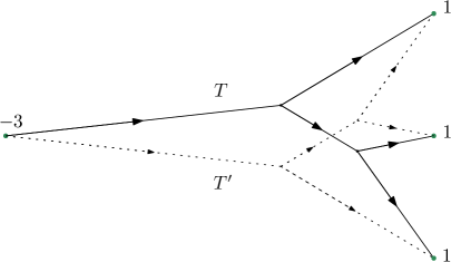
Figure 1. The boundary $\partial T$ is symmetric (with respect to the horizontal axis) and $T\in\textbf{OTP}(\partial T)$ is not symmetric, hence the symmetric copy $T^{\prime}$ is a different minimizer.

The aim of this paper is to prove that for the generic boundary, in the sense of Baire categories, the associated optimal branched transportation problem has a unique minimizer. To this purpose, we denote the set of boundaries by

$${\mathscr{B}}_{0}(K):=\{b\in{\mathscr{D}}_{0}(K):\text{there is an }S\in{\mathscr{D}}_{1}(K)\text{ with }\partial S=b\}\,,$$

we fix an arbitrary constant $C>0$ and we define

$$A_{C}:=\{b\in{\mathscr{B}}_{0}(K):\mathbb{M}(b)\leq C\;{\rm{and}}\;\mathbb{M}^{\alpha}(T)\leq C\mbox{ for every }T\in\textbf{OTP}(b)\}.$$ (1.1)

We metrize $A_{C}$ with the flat norm $\mathbb{F}_{K}$, see (2.2), and we observe that the set $A_{C}$ endowed with the induced distance is a non-trivial complete metric space, see Lemma 2.1. Our main result is the following

Theorem 1.1.

The set of boundaries $b\in A_{C}$, for which $\textbf{OTP}(b)$ is a singleton, is residual.

1.1. Previous results on the well-posedness of the problem

The variational formulations of the optimal branched transportation problem were inspired by the discrete model introduced by Gilbert in [20] and are used to model supply and demand transportation systems which naturally show ramifications as a result of a transportation cost which favors large flows and penalizes diffusion.

In our paper, we adopt the Eulerian formulation proposed by Xia in [32]. Due to a celebrated result by Smirnov, see [31], this is equivalent to the Lagrangian formulation, introduced by Maddalena, Morel and Solimini in [21], see [2, 29]. Existence results and some regularity properties of minimizers have been established for instance in [1, 5, 25, 33, 34]. Recently, another helpful well-posedness property of the problem was established in [14]: the stability of minimizers with respect to variations of the boundary, see [15] for the Lagrangian counterpart. Slightly improving upon the main result of [14], see Theorem A.1, we advance on the study of the well-posedness properties of the branched transportation problem, as we establish the first result on the generic uniqueness of minimizers, in full generality, namely in every dimension $d$ and for every exponent $\alpha\in(0,1)$.

Prior to our work, we are aware of only one elementary result on the uniqueness of minimizing networks. It appeared in the original paper by Gilbert [20], and says that there exists at most one discrete minimum cost communication network with a given Steiner topology.

Several variants and generalizations of the branched transportation problem were proposed and studied by many authors in recent years, see for instance [3, 4, 6, 7, 8, 9, 10, 11, 13, 22, 23, 28, 35]. For the sake of simplicity, we prove the generic uniqueness of minimizers only for the Eulerian formulation introduced in [32].

1.2. Strategy of the proof

Using a small modification of the stability property proved in [14], see Theorem A.1, we show that in order to prove Theorem 1.1, it suffices to prove the density of the set of boundaries $b\in A_{C}$ for which $\textbf{OTP}(b)$ is a singleton, see Lemma 2.2. A similar reduction principle is used in [26, 27] to prove that the generic (higher dimensional) boundary spans a unique minimal hypersurface.

The proof of the density result is based on the following perturbation argument. Firstly, we prove that we can reduce to a finite atomic boundary $b$ with integer multiplicities, exploiting the fact that multiples of such boundaries are dense in $A_{C}$, see Lemma 3.1. For these boundaries, we prove that the solutions to the optimal branched transportation problem are multiples of polyhedral integral currents, see Lemma 3.2. Then we improve the uniqueness result of [20] to suit the discrete branched transportation problem, obtaining as a byproduct that for every finite atomic boundary $b$ as above the set $\textbf{OTP}(b)$ is finite, see Lemma 3.7. We deduce the existence of a set of points $\{p_{1},\dots,p_{h}\}$ in the regular part of the support of a fixed transport path $T\in\textbf{OTP}(b)$ with the property that $T$ is the only element in $\textbf{OTP}(b)$ whose support contains $\{p_{1},\dots,p_{h}\}$, see Lemma 3.8.

Next, we aim to “perturb” the boundary $b$ close to the points $p_{1},\dots,p_{h}$ in order to obtain boundaries with unique minimizers, keeping in mind the fact that the perturbed boundaries should not escape from the set $A_{C}$. More in detail, we define a sequence $(b_{n})_{n\geq 1}\subset A_{C}$ of boundaries for the optimal branched transportation problem with the property that $\mathbb{F}_{K}(b_{n}-b)\to 0$ as $n\to\infty$. Moreover, each $b_{n}$ has points of its support (with small multiplicity) in proximity of $p_{1},\dots,p_{h}$, so that every minimizing transport path $S_{n}$ with boundary $\partial S_{n}=b_{n}$ is forced to have such close-by points in its support. Exploiting again the stability property of Theorem A.1, we deduce that for every choice of $S_{n}\in\textbf{OTP}(b_{n})$ there exists $S\in\textbf{OTP}(b)$ such that, up to subsequences, it holds $\mathbb{F}_{K}(S_{n}-S)\to 0$ and we can infer the Hausdorff convergence of the supports of the $S_{n}$’s to the union of the support of $S$ and the points $p_{1},\dots,p_{h}$, see Lemma 4.2. Notice that at this stage we cannot deduce from Lemma 3.8 that $S=T$, since the portion of $S_{n}$ which is in proximity of some of the $p_{i}$’s might vanish in the limit. In order to exclude this possibility, we perform a fine analysis of the structure of the network $S_{n}$ around the points $p_{1},\dots,p_{h}$, see §4.3: this allows us to exclude all possible local topologies except for two, see (4.18), proving that $p_{1},\dots,p_{h}$ are contained in the support of $S$ (so that in particular $S=T$ by Lemma 3.8) and that $\textbf{OTP}(b_{n})=\{S_{n}\}$, for $n$ sufficiently large, see Lemma 4.3, which concludes the proof of Theorem 1.1.

1.3. Remark.

It is much easier to prove just density in $\bigcup_{C>0}A_{C}$ of the boundaries $b$ for which $\textbf{OTP}(b)$ is a singleton. Indeed, it is significantly simpler to perform the strategy outlined above if one is allowed to choose $b_{n}$ simply satisfying $\mathbb{F}_{K}(b_{n}-b)\to 0$ and $\mathbb{M}^{\alpha}(S_{n})\leq C$, but possibly with $\mathbb{M}(b_{n})>C$: for instance it suffices to choose the perturbation $b_{n}$ as in (4.1) with $k=1$, in which case it is easy to prove that $\textbf{OTP}(b_{n})$ is a singleton. Obviously such type of perturbation is not admissible in order to prove the residuality result of Theorem 1.1, since such boundaries $b_{n}$ do not belong to $A_{C}$. One of the challenges in our proof is therefore to find suitable perturbations $b_{n}$ of $b$ which are internal to the set $A_{C}$ and such that for the boundary $b_{n}$ there exists a unique minimizer of the optimal branched transportation problem, for $n$ sufficiently large.

1.4. Remark.

Following [26, 27], it would be tempting to adopt a seemingly simpler strategy to prove Theorem 1.1. Indeed the density result would be an easy consequence of the following unique continuation principle: if $b$ is a finite atomic boundary with integer multiplicities, then any two elements of $\textbf{OTP}(b)$ which coincide on a neighbourhood of the support of $b$ necessarily coincide globally.
One reason to believe that such a statement could be true is the fact that, knowing the directions and the multiplicities of all the edges colliding at a branch point except for one, it is possible to deduce the information on the last edge, by exploiting a balancing condition which is due to the stationarity of the network for the $\alpha$-mass. The main obstruction to prove the statement is the following. If for a minimizer $T$ in $\textbf{OTP}(b)$ two or more edges emanating from the boundary collide at some branch point, it is not obvious that for another minimizer $T^{\prime}$ which coincides with $T$ on a neighbourhood of the support of $b$ the same edges still collide: it might happen that $T^{\prime}$ has some branch point in the interior of one of these edges. We do not exclude that the statement could be true, but we believe that this cannot be proved only by local properties, which would make a potential proof quite involved. This is the reason why we opted for a completely different strategy, which is based ultimately on local arguments only.
The presence of singularities is not an issue in the framework of minimal surfaces, because the singular set is too small to disconnect the regular part of the surface. We believe that the strategy which we devised is of general interest and can be adapted to prove generic uniqueness of solutions to other variational problems with large singular sets, see [17, 18].

2. Preliminaries

Through the paper $K\subset$ $\mathbb{R}^{d}$ denotes a convex compact set. We denote by $\mathscr{M}(K)$ the space of signed Radon measures on $K$ and by $\mathscr{M}_{+}(K)$ the subspace of positive measures. The total variation measure associated to a measure $\mu\in\mathscr{M}(K)$ is denoted by $\|\mu\|$ and $\mu_{+}:=1/2(\|\mu\|+\mu)$ and $\mu_{-}:=1/2(\|\mu\|-\mu)$ denote respectively the positive and the negative part of $\mu$. The mass of $\mu$ is the quantity $\mathbb{M}(\mu):=\|\mu\|(K)$. We say that a measure is finite atomic if its support is a finite set.

We adopt Xia’s Eulerian formulation [32] of the optimal branched transportation problem. This employs the theory of currents, for which we refer the reader to [19]. We recall that a $k$-dimensional current on $\mathbb{R}^{d}$ is a continuous linear functional on the space $\mathscr{D}^{k}(\mathbb{R}^{d})$ of smooth and compactly supported differential $k$-forms and we denote by $\mathscr{D}_{k}(K)$ the space of $k$-dimensional currents with support in $K$. The space $\mathscr{D}_{k}(K)$ is endowed with a norm which is called mass and denoted by $\mathbb{M}$. By the Riesz representation theorem, a current $T$ with $\mathbb{M}(T)<\infty$ can be identified with vector-valued Radon measures $\vec{T}\mu_{T}$ where $\vec{T}$ is a unit $k$-vector field and $\mu_{T}$ a positive Radon measure. The mass of the current $T$ coincides with the mass of the measure $\mu_{T}$. We denote by $\mathrm{supp}(T)$ the support of a current $T$, which coincides with the support of the measure $\mu_{T}$, if $T$ has finite mass. The boundary of a current $T\in\mathscr{D}_{k}(K)$ is the current $\partial T\in\mathscr{D}_{k-1}(K)$ such that

$$\partial T(\phi)=T(d\phi),\quad\mbox{ for every $\phi\in\mathscr{D}^{k-1}(\mathbb{R}^{d})$}.$$

A current $T$ such that $\mathbb{M}(T)+\mathbb{M}(\partial T)<\infty$ is called a normal current. The space of $k$-dimensional normal currents with support in $K$ is denoted by $\mathscr{N}_{k}(K)$.

We say that a current $T\in\mathscr{D}_{k}(K)$ is rectifiable and we write $T\in\mathscr{R}_{k}(K)$ if we can identify $T$ with a triple $(E,\tau,\theta)$, where $E\subset K$ is a $k$-rectifiable set, $\tau(x)$ is a unit $k$-vector spanning the tangent space Tan$(E,x)$ at $\mathscr{H}^{k}$-a.e. $x$ and $\theta\in L^{1}(\mathscr{H}^{k}\mathchoice{\mathbin{\vrule width=0.51663pt,height=5.16663pt,depth=0.12915pt\vrule width=3.44444pt,height=0.38748pt,depth=0.12915pt}}{\mathbin{\vrule width=0.51663pt,height=5.16663pt,depth=0.12915pt\vrule width=3.44444pt,height=0.38748pt,depth=0.12915pt}}{\mathbin{\hskip 0.6458pt\vrule width=0.38748pt,height=3.61664pt,depth=0.08612pt\vrule width=2.41109pt,height=0.3014pt,depth=0.08612pt}\hskip 0.6458pt}{\mathbin{\vrule width=0.3014pt,height=2.58334pt,depth=0.04303pt\vrule width=1.72218pt,height=0.25832pt,depth=0.04303pt}}E)$, where the identification means that

$$T(\omega)=\int_{E}\langle\omega(x),\tau(x)\rangle\theta(x)d\mathscr{H}^{k}(x),\quad\mbox{ for every $\omega\in\mathscr{D}^{k}(\mathbb{R}^{d})$}.$$

Those currents $T=(E,\tau,\theta)$ which are normal and rectifiable with integer multiplicity $\theta$ are called integral currents. The subgroup of integral currents with support in $K$ is denoted by $\mathscr{I}_{k}(K)$.

A $k$-dimensional polyhedral current is a current $P$ of the form

$$P:=\sum_{i=1}^{N}\theta_{i}\llbracket\sigma_{i}\rrbracket,$$ (2.1)

where $\theta_{i}\in\mathbb{R}\setminus\{0\}$, $\sigma_{i}$ are nontrivial $k$-dimensional simplexes in $\mathbb{R}^{d}$, with disjoint relative interiors, oriented by $k$-vectors $\tau_{i}$ and $\llbracket\sigma_{i}\rrbracket=(\sigma_{i},\tau_{i},1)$ is the multiplicity-one rectifiable current naturally associated to $\sigma_{i}$. The subgroup of polyhedral currents with support in $K$ is denoted $\mathscr{P}_{k}(K)$. A polyhedral current with integer coefficients $\theta_{i}$ is called integer polyhedral.

Given $\alpha\in(0,1)$ and a 1-current $T\in\mathscr{N}_{1}(K)\cup\mathscr{R}_{1}(K)$ we define the $\alpha$-mass

$$\mathbb{M}^{\alpha}(T):=\begin{cases}\int_{E}|\theta|^{\alpha}d\mathscr{H}^{1},&\text{if}\ T=(E,\tau,\theta)\in\mathscr{R}_{1}(K);\\ +\infty,&\text{otherwise.}\end{cases}$$

If $\mu_{-}$ and $\mu_{+}$ are elements of $\mathscr{M}_{+}(K)$ such that $\mathbb{M}(\mu_{-})=\mathbb{M}(\mu_{+})$, the optimal branched transportation problem with boundary $b=\mu_{+}-\mu_{-}$ seeks a normal current $T\in\mathscr{N}_{1}(K)$ which minimizes the $\alpha$-mass $\mathbb{M}^{\alpha}$ among all currents $S$ with boundary $\partial S=b$. Hence, we denote by $\textbf{TP}(b)$ the set of transport paths with boundary $b$ as

$$\textbf{TP}(b):=\{T\in\mathscr{N}_{1}(K):\partial T=b\},$$

and the least transport energy associated to $b$ as

$$\mathbb{E}^{\alpha}(b):=\inf\{\mathbb{M}^{\alpha}(T):T\in\textbf{TP}(b)\}.$$

We define the set of optimal transport paths with boundary $b$ by

$$\textbf{OTP}(b):=\{T\in\textbf{TP}(b):\mathbb{M}^{\alpha}(T)=\mathbb{E}^{\alpha}(b)\}.$$

Let $A_{C}$ be the set of boundaries defined in (1.1). Due to the Baire category theorem, the next lemma ensures that a residual subset of $A_{C}$ (namely a set which contains a countable intersection of open dense subsets) is dense. We recall that the flat norm $\mathbb{F}_{K}(T)$ of a current $T\in\mathscr{D}_{k}(K)$ is the following quantity, see [19, §4.1.12],

$$\mathbb{F}_{K}(T):=\inf\{\mathbb{M}(T-\partial S)+\mathbb{M}(S):S\in\mathscr{D}_{k+1}(K)\}.$$ (2.2)

Lemma 2.1.

The set $A_{C}$ is $\mathbb{F}_{K}$-closed. In particular $(A_{C},\mathbb{F}_{K})$ is a complete metric space.

• The second part of the statement follows from the first part and from the $\mathbb{F}_{K}$-compactness of 0-currents with support in $K$ and mass bounded by $C$, see [19, §4.2.17].

  In order to prove that $A_{C}$ is $\mathbb{F}_{K}$ closed, let $(b_{j})_{j\in\mathbb{N}}$ be a sequence of elements of $A_{C}$ and let $b$ be such that $\mathbb{F}_{K}(b_{j}-b)\to 0$ as $j\to\infty$. We want to prove that $b\in A_{C}$. By the lower semicontinuity of the mass (with respect to the flat convergence), we have $\mathbb{M}(b)\leq C$. For any $j\in\mathbb{N}$, let $T_{j}\in\textbf{OTP}(b_{j})$. By [12, Proposition 3.6], we have $\mathbb{M}(T_{j})\leq C^{1-\alpha}\mathbb{M}^{\alpha}(T_{j})\leq C^{2-\alpha}$. By the compactness theorem for normal currents, there exists $T\in{\mathscr{N}}_{1}(K)$ such that, up to (non relabeled) subsequences $\mathbb{F}_{K}(T_{j}-T)\to 0$. By the continuity of the boundary operator we have $\partial T=b$ and by the lower semicontinuity of the $\alpha$-mass, see [16], we have $\mathbb{M}^{\alpha}(T)\leq C$ and hence $b\in A_{C}$. ∎

Consider the following subset of $A_{C}$, which represents the set of boundaries admitting non-unique minimizers:

$$NU_{C}:=\{b\in A_{C}:\exists\,\,T^{1},T^{2}\in\textbf{OTP}(b)\text{ such that }T^{1}\neq T^{2}\}.$$

Notice that since $b\in A_{C}$ then $\mathbb{M}^{\alpha}(T^{1})=\mathbb{M}^{\alpha}(T^{2})\leq C$. We have the following:

Lemma 2.2.

Assume that the set $A_{C}\setminus NU_{C}$ is $\mathbb{F}_{K}$-dense in $A_{C}$. Then it is residual.

• For $m\in\mathbb{N}\setminus\{0\}$, consider the sets

  $$NU_{C}^{m}:=\{b\in A_{C}:\exists\,\{T^{1},T^{2}\}\subset\textbf{OTP}(b)\;{\rm with}\;\mathbb{F}_{K}(T^{2}-T^{1})\geq m^{-1}\}.$$

  Since $NU_{C}^{m}\subset NU_{C}$, then $(A_{C}\setminus NU_{C}^{m})\supset(A_{C}\setminus NU_{C})$ and hence, by assumption, $A_{C}\setminus NU_{C}^{m}$ is $\mathbb{F}_{K}$-dense in $A_{C}$ for every $m$. Therefore $NU_{C}^{m}$ has empty interior in $A_{C}$ for every $m$.

  To conclude, it is sufficient to prove that $NU_{C}^{m}$ is closed for every $m$. Consider a sequence $(b_{j})_{j\in\mathbb{N}}$ of elements of $NU_{C}^{m}$ and let $b\in A_{C}$ be such that $\mathbb{F}_{K}(b_{j}-b)\to 0$. We need to prove that $b\in NU_{C}^{m}$. For every $j\in\mathbb{N}$, take

  $$\{T^{1}_{j},T^{2}_{j}\}\subset\textbf{OTP}(b_{j})\quad{\mbox{ with }}\quad\mathbb{F}_{K}(T^{2}_{j}-T^{1}_{j})\geq m^{-1}.$$

  As in the proof of Lemma 2.1, we deduce that there exist $T^{1},T^{2}\in{\mathscr{N}}_{1}(K),$ such that $\partial T^{1}=\partial T^{2}=b$ and, up to (non relabeled) subsequences, $\mathbb{F}_{K}(T^{1}_{j}-T^{1})\to 0$, $\mathbb{F}_{K}(T^{2}_{j}-T^{2})\to 0$ as $j\to\infty$. Clearly $\mathbb{F}_{K}(T^{2}-T^{1})\geq m^{-1}$. By Theorem A.1, we have $\{T_{1},T_{2}\}\subset\textbf{OTP}(b)$, hence $b\in NU_{C}^{m}$. ∎

3. Density of boundaries with unique minimizers: preliminary reductions

3.1. Reduction to integral boundaries and integer polyhedral minimizers

Lemma 3.1.

For any $b\in A_{C}$ and $\varepsilon>0$, there exist $\delta>0$ and a boundary $b^{\prime\prime}\in A_{C-\delta}$ with

$$\mathbb{F}_{K}(b-b^{\prime\prime})<\varepsilon\qquad\text{ and }\qquad b^{\prime\prime}=\eta b_{I}$$

for some $\eta>0$ and $b_{I}\in\mathscr{I}_{0}(K)$.

• Without loss of generality and up to rescaling, we can assume $C=1$ and write $A$ instead of $A_{C}$. Let $b\in A$ and $T\in\textbf{OTP}(b)$ and define $T_{\varepsilon}:=(1-\varepsilon/4)T$. Then $b_{\varepsilon}:=\partial T_{\varepsilon}=(1-\varepsilon/4)b$ and $T_{\varepsilon}\in\textbf{OTP}(b_{\varepsilon})$ satisfy

  $$\mathbb{M}^{\alpha}(T_{\varepsilon})\leq(1-\varepsilon/4)^{\alpha}\quad\mbox{ and }\quad\mathbb{M}(b_{\varepsilon})\leq 1-\varepsilon/4.$$ (3.1)

  Since we also have $\mathbb{M}(b-b_{\varepsilon})\leq\varepsilon/4$, we deduce that

  $$\mathbb{F}_{K}(b-b_{\varepsilon})\leq\varepsilon/4.$$ (3.2)

  Now apply [24, Theorem 5] to obtain, possibly after rescaling, a current $T^{\prime}_{\varepsilon}\in\mathscr{P}_{1}(K)$, such that, denoting $b^{\prime}_{\varepsilon}:=\partial T^{\prime}_{\varepsilon}$, we have

  $$\mathbb{M}^{\alpha}(T^{\prime}_{\varepsilon})\leq\mathbb{M}^{\alpha}(T_{\varepsilon}),\quad\mathbb{M}(b^{\prime}_{\varepsilon})\leq\mathbb{M}(b_{\varepsilon})\quad\mbox{and}\quad\mathbb{F}_{K}(T^{\prime}_{\varepsilon}-T_{\varepsilon})\leq\varepsilon/4,$$ (3.3)

  and in particular $\mathbb{F}_{K}(b^{\prime}_{\varepsilon}-b_{\varepsilon})\leq\varepsilon/4$. We can write

  $$T^{\prime}_{\varepsilon}=\sum_{i=1}^{N}\theta_{i}^{\prime}\llbracket\sigma_{i}\rrbracket$$

  as in (2.1). Up to changing the orientation of $\llbracket\sigma_{i}\rrbracket$, we may assume $\theta^{\prime}_{i}>0$ for every $i$. Fix $\eta:=\varepsilon/(16N)$ and denote $\theta_{i}^{\prime\prime}:=\eta\left\lfloor\frac{\theta_{i}^{\prime}}{\eta}\right\rfloor$ (where $\lfloor x\rfloor$ is the largest integer smaller than or equal to $x$) so that

  $$0\leq\theta_{i}^{\prime}-\theta_{i}^{\prime\prime}<\frac{\varepsilon}{16N}\qquad\mbox{for every $i\in\{1,\dots,N\}$}.$$ (3.4)

  Define

  $$T^{\prime\prime}:=\sum_{i=1}^{N}\theta_{i}^{\prime\prime}\llbracket\sigma_{i}\rrbracket$$

  and denote $b^{\prime\prime}=\partial T^{\prime\prime}$. Observe that by (3.4) and (3.3) we have

  $$\mathbb{M}^{\alpha}(T^{\prime\prime})\leq\mathbb{M}^{\alpha}(T^{\prime}_{\varepsilon})\leq\mathbb{M}^{\alpha}(T_{\varepsilon})<1.$$ (3.5)

  For every $i\in\{1,\dots,N\}$, we denote by $x_{i}$ and $y_{i}$ respectively the first and second endpoint of the oriented segment $\sigma_{i}$, so that we can write

  $$b^{\prime}_{\varepsilon}=\sum_{i=1}^{N}\theta_{i}^{\prime}(\delta_{y_{i}}-\delta_{x_{i}})$$

  which we can rewrite as

  $$b^{\prime}_{\varepsilon}=\sum_{j=1}^{M}\beta_{j}^{\prime}\delta_{z_{j}},$$

  where all points $z_{j}$ are distinct and

  $$\beta_{j}^{\prime}:=\left(\sum_{\{i:y_{i}=z_{j}\}}\theta_{i}^{\prime}-\sum_{\{i:x_{i}=z_{j}\}}\theta_{i}^{\prime}\right).$$

  Analogously, we define

  $$\beta_{j}^{\prime\prime}:=\left(\sum_{\{i:y_{i}=z_{j}\}}\theta_{i}^{\prime\prime}-\sum_{\{i:x_{i}=z_{j}\}}\theta_{i}^{\prime\prime}\right),$$

  so that we can write

  $$b^{\prime\prime}=\sum_{j=1}^{M}\beta_{j}^{\prime\prime}\delta_{z_{j}}.$$

  Thus we obtain

  $$\begin{split}\mathbb{M}(b^{\prime\prime}-b^{\prime}_{\varepsilon})=\sum_{j=1}^{M}|\beta_{j}^{\prime\prime}-\beta_{j}^{\prime}|\leq\Bigg{|}\sum_{\{i:x_{i}=z_{j}\}}(\theta_{i}^{\prime\prime}-\theta_{i}^{\prime})\Bigg{|}+\Bigg{|}\sum_{\{i:y_{i}=z_{j}\}}(\theta_{i}^{\prime\prime}-\theta_{i}^{\prime})\Bigg{|}\stackrel{{\scriptstyle(\ref{e:appx})}}{{<}}\frac{\varepsilon}{16}+\frac{\varepsilon}{16}=\frac{\varepsilon}{8}\end{split}$$ (3.6)

  and by (3.1) and (3.3) we deduce

  $$\mathbb{M}(b^{\prime\prime})\leq\mathbb{M}(b^{\prime}_{\varepsilon})+\mathbb{M}(b^{\prime\prime}-b^{\prime}_{\varepsilon})<1.$$ (3.7)

  Combining (3.6) with (3.2) and (3.3), we get $\mathbb{F}_{K}(b-b^{\prime\prime})<\varepsilon$. The conclusion follows denoting $b_{I}:=\eta^{-1}b^{\prime\prime}$ and observing that $b_{I}\in\mathscr{I}_{0}(K)$ (as the $\theta^{\prime\prime}_{i}$ are multiples of $\eta$) and that by (3.5) and (3.7) we have $b^{\prime\prime}\in A_{1-\delta}$ for some $\delta>0$. ∎

Lemma 3.2.

If $b\in\mathscr{I}_{0}(K)$ and $T\in\mathscr{N}_{1}(K)$ is in $\textbf{OTP}(b)$ then $T\in\mathscr{P}_{1}(K)\cap\mathscr{I}_{1}(K)$.

• Combining the good decomposition properties of optimal transport paths [12, Proposition 3.6] and their single path property [2, Proposition 7.4] with the assumption $\partial T\in\mathscr{P}_{0}(K)$, we deduce that there are finitely many Lipschitz simple paths $\gamma_{1},\dots,\gamma_{N}$ of finite length such that $T$ can be written as a $T=\sum_{i=1}^{N}a_{i}\llbracket\gamma_{i}\rrbracket$, where $a_{i}>0$ for every $i$ and $\llbracket\gamma_{i}\rrbracket\in\mathscr{I}_{1}(K)$ is the current $({\rm{Im}}(\gamma_{i}),\gamma_{i}^{\prime}/|\gamma_{i}^{\prime}|,1)$. Moreover, again by [2, Proposition 7.4], one can assume that ${\rm{Im}}(\gamma_{i})\cap{\rm{Im}}(\gamma_{j})$ is connected for every $i,j$, which in turn implies that $T\in\mathscr{P}_{1}(K)$. Hence we can write

  $$T:=\sum_{\ell=1}^{N}\theta_{\ell}\llbracket\sigma_{\ell}\rrbracket,$$

  where $\sigma_{\ell}$ are non-overlapping oriented segments and $\theta_{\ell}\in\mathbb{R}$. We want to prove that $\theta_{\ell}\in\mathbb{Z},\forall\ell$.

  Denote

  $$\mathcal{I}:=\{\ell\in\{1,\dots,N\}:\theta_{\ell}\in\mathbb{R}\setminus\mathbb{Z}\}$$

  and let $\hat{T}:=\sum_{\ell\in\mathcal{I}}\theta_{\ell}\llbracket\sigma_{\ell}\rrbracket$. Assume by contradiction that $\hat{T}\neq 0$. Note that $T-\hat{T}\in\mathscr{I}_{1}(K)$ and therefore, since $b\in\mathscr{I}_{0}(K)$, we have $\partial\hat{T}=b-\partial(T-\hat{T})\in\mathscr{I}_{0}(K)$. Hence, for every point $x$ in the support of $\partial\hat{T}$ there are at least two distinct segments $\sigma_{\ell_{1}}$ and $\sigma_{\ell_{2}}$ having $x$ as an endpoint. This implies that the support of $\hat{T}$, and in particular also the support of $T$, contains a loop, which contradicts [2, Proposition 7.8]. ∎

3.2. Finiteness of the set of minimizers for an integral boundary

Definition 3.3 (Topology and branch points).

Let $b\in\mathscr{I}_{0}(K)$ and let $T,T^{\prime}\in\mathscr{P}_{1}(K)$ with $\partial T=\partial T^{\prime}=b$. We say that $T$ and $T^{\prime}$ have the same topology if there exist two ordered sets, each made of distinct points, $\{x_{1},\dots,x_{M}\}$ and $\{x^{\prime}_{1},\dots,x^{\prime}_{M}\}$ with the following properties:

• for every $p\in\mathrm{supp}(b)$ there exists $i$ such that $x_{i}=p=x^{\prime}_{i}$;

• denoting $\sigma_{ij}$ the segment with first endpoint $x_{i}$ and second endpoint $x_{j}$ and $\sigma^{\prime}_{ij}$ the segment with first endpoint $x^{\prime}_{i}$ and second endpoint $x^{\prime}_{j}$, $T$ and $T^{\prime}$ can be written respectively as

  $$T=\sum_{i<j}a_{ij}\llbracket\sigma_{ij}\rrbracket,\quad T^{\prime}=\sum_{i<j}a^{\prime}_{ij}\llbracket\sigma^{\prime}_{ij}\rrbracket,\quad\mbox{ for some $a_{ij},a^{\prime}_{ij}\in\mathbb{R}$.}$$ (3.8)

• the representations in (3.8), restricted to the nonzero addenda, is of the same type as (2.1). In particular, if $a_{ij}$ and $a_{kl}$ (resp. $a^{\prime}_{ij}$ and $a^{\prime}_{kl}$) are nonzero, then $\sigma_{ij}$ and $\sigma_{kl}$ (resp. $\sigma^{\prime}_{ij}$ and $\sigma^{\prime}_{kl}$) have disjoint interiors. Moreover, the number of nonzero addenda in the representation of $T$ (resp. $T^{\prime}$) given in (3.8) coincides with the smallest number $N$ for which $T$ (resp. $T^{\prime}$) can be written as in (2.1).

• $a_{ij}=0$ if and only if $a^{\prime}_{ij}=0$. In particular, the number $N$ of the previous point is the same for $T$ and $T^{\prime}$.

One can check that the above conditions define an equivalence relation on the set of polyhedral currents. We call the topology of a polyhedral current $T$ the corresponding equivalence class. Notice that the number $M$ depends only on the equivalence class and for every $T$ the (unordered) set $\{x_{1},\dots,x_{M}\}$ is uniquely determined, by property (iii). The set $\{x_{1},\dots,x_{M}\}\setminus\mathrm{supp}(b)$ is called the set of branch points of $T$ and denoted by $\textbf{BR}(T)$. By Lemma 3.2, for every $T\in\textbf{OTP}(b)$ the topology of $T$ and the set $\textbf{BR}(T)$ are well defined.

Lemma 3.4.

Let $0\neq b\in\mathscr{I}_{0}(K)$ and $T\in\textbf{OTP}(b)$. Then $\mathscr{H}^{0}(\textbf{BR}(T))\leq\mathscr{H}^{0}(\mathrm{supp}(b))-2$.

• Suppose without loss of generality that $\mathscr{H}^{0}(\textbf{BR}(T))>0$. Assume by contradiction that the lemma is false and let $n$ be the minimal number such that there exist $b\in\mathscr{I}_{0}(K)$ and $T\in\textbf{OTP}(b)$ such that

  $$\mathscr{H}^{0}(\textbf{BR}(T))+2>n=\mathscr{H}^{0}(\mathrm{supp}(b)).$$

  Notice that $n>2$. Fix $p\in\textbf{BR}(T)$ and let $\varepsilon>0$ be such that

  $$(\overline{B}_{\varepsilon}(p)\setminus\{p\})\cap(\mathrm{supp}(b)\cup\textbf{BR}(T))=\emptyset.$$

  Denote by $T_{1},\dots,T_{m}$ the restriction of $T$ to the connected components of $\mathrm{supp}(T)\setminus B_{\varepsilon}(p)$. We notice that $m\geq 3$. Indeed, if $m=1$ we would have the contradiction $p\in\mathrm{supp}(b)$ and if $m=2$, writing $T$ as in (3.8), the only two segments with nonzero coefficient having $p$ as an endpoint cannot be collinear by property (iii): this contradicts the the fact that $T\in\textbf{OTP}(b)$. Observe that for every $i$ we have that $\mathrm{supp}(\partial T_{i})\setminus\mathrm{supp}(b)$ consists of exactly one point $p_{i}$, so that

  $$n=\sum_{i=1}^{m}\left(\mathscr{H}^{0}(\mathrm{supp}(\partial T_{i}))-1\right).$$ (3.9)

  By minimality of $n$ and the fact that $m\geq 3$, we have

  $$\mathscr{H}^{0}(\textbf{BR}(T_{i}))\leq\mathscr{H}^{0}(\mathrm{supp}(\partial T_{i}))-2\quad\text{ for all $i\in\{1,\dots,m\}$}.$$ (3.10)

  Since $m\geq 3$, the combination of (3.9) and (3.10) leads to a contradiction. ∎

Lemma 3.5.

Let $b\in\mathscr{I}_{0}(K)$ and let $T,T^{\prime}\in\mathscr{P}_{1}(K)$ with $\partial T=b=\partial T^{\prime}$ have the same topology. Assume moreover that $\mathrm{supp}(T)$ and $\mathrm{supp}(T^{\prime})$ do not contain loops. Write $T$ and $T^{\prime}$ as in (3.8) with properties (i)-(iv) and with the same orientation on each segment. Then $a_{ij}=a^{\prime}_{ij}$ for every $i,j$.

• By contradiction, let $T,T^{\prime}$ be nonzero currents with the same topology, $\partial T=b=\partial T^{\prime}$, and minimizing the quantity $M$ in Definition 3.3 among all pairs for which the lemma is false. We claim that there exists a point $p\in\mathrm{supp}(b)$ and (up to reordering) indexes $i,j\in\{1,\dots,M\}$ such that

  • $a_{lj}=0=a^{\prime}_{lj}$ for every $l\neq i$;

  • $x_{j}=p=x^{\prime}_{j}$ and $a_{ij}\neq a^{\prime}_{ij}$, with $a_{ij},a^{\prime}_{ij}\in\mathbb{R}\setminus\{0\}$.

  The validity of (a) follows from the absence of loops. On the other hand, if a point $p$ as in (a) violated (b), one could restrict the currents $T$ and $T^{\prime}$ respectively to the complementary of $\sigma_{ij}$ and $\sigma^{\prime}_{ij}$, thus contradicting the minimality of $M$. The validity of (a) and (b) is a contradiction because the multiplicities $a_{ij}$ and $a^{\prime}_{ij}$ correspond to the multiplicity of $p$ as point in the support of $b$. ∎

Lemma 3.6.

Let $b\in\mathscr{I}_{0}(K)$ and $S,T\in\textbf{OTP}(b)$ with $\mathrm{supp}(S)=\mathrm{supp}(T)$. Then $S=T$.

• Assume by contradiction $S\neq T$. By Lemma 3.2, $S-T\in\mathscr{P}_{1}(K)\cap\mathscr{I}_{1}(K)$ is a nontrivial current with $\partial(S-T)=0$ and by assumption $\mathrm{supp}(S-T)\subset\mathrm{supp}(S)$. As in the proof of Lemma 3.2 we deduce that $\mathrm{supp}(S-T)$ contains a loop. In particular, so does $\mathrm{supp}(S)$, which contradicts [2, Proposition 7.8]. ∎

Lemma 3.7.

Let $b\in\mathscr{I}_{0}(K)$ be a boundary. Then $\textbf{OTP}(b)$ is finite.

• By Lemma 3.4 the range of the integer $M$ of Definition 3.3 among all $T\in\textbf{OTP}(b)$ is finite. In turn this implies that the set of possible topologies of currents $T\in\textbf{OTP}(b)$ is finite. Indeed the topology of a polyhedral current $T$ as in Definition 3.3, up to choosing the order of the points $\{x_{1},\dots,x_{M}\}$, is uniquely determined by the $M\times M$ matrix $A:=(|{\rm{sign}}(a_{ij})|)_{ij}$. Hence it is sufficient to prove that if $T$ and $T^{\prime}$ are in $\textbf{OTP}(b)$ and have the same topology, then $T=T^{\prime}$, and by Lemma 3.6 it suffices to prove that $\mathrm{supp}(T)=\mathrm{supp}(T^{\prime})$.

  By [2, Proposition 7.8] the support of $T$ and $T^{\prime}$ does not contain loops, hence we can apply Lemma 3.5 and we can assume that $T$ and $T^{\prime}$ can be written as in (3.8) with $a_{ij}=a^{\prime}_{ij}$ for every $i,j=1,\dots,M$. This means that the set of competitors for the branched transportation problem with boundary $b$ and a given topology can be reduced to a family of polyhedral currents $T\in\mathscr{P}_{1}(K)$ whose only unknown is the position of the points $\{x_{1},\dots,x_{M}\}\setminus\mathrm{supp}(b)$. Accordingly, we denote $n:=\mathscr{H}^{0}(\mathrm{supp}(b))$ and we order the points $\{x_{1},\dots,x_{M}\}$ in such a way that $\textbf{BR}(T)=\{x_{1},\dots,x_{M-n}\}$. The $\alpha$-mass of such $T$ is computed as

  $$\mathbb{M}^{\alpha}(T)=\sum_{i<j}|a_{ij}|^{\alpha}\mathscr{H}^{1}(\sigma_{ij})$$

  and by the previous discussion, since the vector $(x_{M-n+1},\dots,x_{M})$ is fixed, this is a functional of the vector $(x_{1},\dots,x_{M-n})$ only, which can be written as

  $$\mathbb{M}^{\alpha}(T)=F(x_{1},\dots,x_{M-n}):=\sum_{i<j}|a_{ij}|^{\alpha}|x_{j}-x_{i}|=C+\sum_{i=1}^{M-n}\sum_{j=i+1}^{M}|a_{ij}|^{\alpha}|x_{j}-x_{i}|,$$ (3.11)

  where $C=\sum_{i=M-n+1}^{M}\sum_{i<j}|a_{ij}|^{\alpha}|x_{j}-x_{i}|$. One can immediately see that $F$ is convex, being a sum of convex functions. Moreover each term $|a_{ij}|^{\alpha}|x_{j}-x_{i}|$ in (3.11), as a function of the variable $x_{j}$, is strictly convex on a segment $[s,t]$ whenever $x_{i}$, $s$ and $t$ are not collinear.

  Assume by contradiction that $T\neq T^{\prime}\in\textbf{OTP}(b)$ have the same topology and consider the corresponding sets

  $$\textbf{BR}(T)=\{x_{1},\dots,x_{M-n}\},\quad\textbf{BR}(T^{\prime})=\{x^{\prime}_{1},\dots,x^{\prime}_{M-n}\}.$$

  By Lemma 3.5 there exists $j\in\{1,\dots,M-n\}$ such that $x_{j}\neq x^{\prime}_{j}$. As in the proof of Lemma 3.4 we infer that $x_{j}$ is an endpoint of at least three segments in the support of $T$ which are not collinear. We deduce by the discussion after (3.11) that the function $F$ is strictly convex in the $j$-th variable. Since $F(x_{1},\dots,x_{M-n})=F(x^{\prime}_{1},\dots,x^{\prime}_{M-n})$ we deduce that there exists a point $(y_{1},\dots,y_{M-n})$ with

  $$F(y_{1},\dots,y_{M-n})<F(x_{1},\dots,x_{M-n}).$$ (3.12)

  Denote

  $$z_{i}:=\begin{cases}y_{i}\quad\mbox{if $i\leq M-n$}\\ x_{i}\quad\mbox{otherwise}\end{cases}$$

  and let $S$ be the current

  $$S:=\sum_{i<j}a_{ij}\llbracket\tilde{\sigma}_{ij}\rrbracket,$$ (3.13)

  where $\tilde{\sigma}_{ij}$ is the segment with first endpoint $z_{i}$ and second endpoint $z_{j}$. Notice that in principle it might happen that $S$ does not have the same topology as $T$ and $T^{\prime}$, since (3.13) might fail to have property (iii) of Definition 3.3. However we have $\partial S=b$ and by (3.12)

  $$\mathbb{M}^{\alpha}(S)\leq F(y_{1},\dots,y_{M-n})<F(x_{1},\dots,x_{M-n})=\mathbb{M}^{\alpha}(T),$$

  which contradicts the assumption $T\in\textbf{OTP}(b)$. ∎

Lemma 3.8.

For every boundary $b\in\mathscr{I}_{0}(K)$ and $T\in\textbf{OTP}(b)$, there is a set of distinct points $\{p_{1},\dots,p_{h}\}\subset\mathrm{supp}(T)\setminus(\textbf{BR}(T)\cup\mathrm{supp}(b))$ such that

$$\big{\{}S\in\textbf{OTP}(b):\{p_{1},\dots,p_{h}\}\subset\mathrm{supp}(S)\big{\}}=\{T\}\,.$$

Moreover, the $p_{i}$’s can be chosen so that if $p_{i}\in\mathrm{supp}(T)\cap\mathrm{supp}(S)$ for some $S\in\textbf{OTP}(b)$, then there exists $\rho>0$ such that $\mathrm{supp}(T)\cap B_{\rho}(p_{i})=\mathrm{supp}(S)\cap B_{\rho}(p_{i})$.

• By Lemma 3.7 we have that $\textbf{OTP}(b)$ consists of finitely many polyhedral currents $T^{1},\dots,T^{h}$ and, by Lemma 3.6, the symmetric difference $\mathrm{supp}(T^{i})\triangle\,\mathrm{supp}(T^{j})$ is a relatively open set of positive length for every $i\neq j$. Up to reordering, we assume $T^{1}=T$ and for every $i\in\{2,\dots,h\}$ we consider the set $U_{i}:=\mathrm{supp}(T)\setminus(\mathrm{supp}(T^{i})\cup\textbf{BR}(T))$. We observe, recalling that $\textbf{BR}(T)$ is finite by Lemma 3.4, that each $U_{i}$ is relatively open with positive length. Define the subset

  $$V_{i}:=U_{i}\cap\Big{(}\bigcup_{j\neq i}\textbf{BR}(T^{j})\cup\left\{p\in U_{i}:\text{$\mathrm{supp}(T^{j})$ intersects $U_{i}$ transversally at $p$}\right\}\Big{)}$$

  and observe that $V_{i}$ is finite since every $T^{j}$ is polyhedral. Then choose $p_{i}\in U_{i}\setminus V_{i}$. Clearly $p_{i}\in\mathrm{supp}(T)\setminus(\textbf{BR}(T)\cup\mathrm{supp}(b))$ and $p_{i}\not\in\mathrm{supp}(T^{i})$; moreover if $p_{i}\in\mathrm{supp}(T^{j})$ then locally $\mathrm{supp}(T^{j})$ agrees with $\mathrm{supp}(T)$. ∎

4. Density of boundaries with unique minimizers: perturbation argument

4.1. Construction of the perturbed boundaries

Let us fix a boundary $b\in\mathscr{I}_{0}(K)$, an integer polyhedral current $T\in\textbf{OTP}(b)$, see Lemma 3.2, and points $\{p_{1},\dots,p_{h}\}$ as in Lemma 3.8. For a fixed $k\in\mathbb{N}\setminus\{0\}$ and for $n=1,2,\dots$ we denote

$$\begin{split}T_{n}&:=T-\frac{1}{k}\sum_{i=1}^{h}T\mathchoice{\mathbin{\vrule width=0.51663pt,height=5.16663pt,depth=0.12915pt\vrule width=3.44444pt,height=0.38748pt,depth=0.12915pt}}{\mathbin{\vrule width=0.51663pt,height=5.16663pt,depth=0.12915pt\vrule width=3.44444pt,height=0.38748pt,depth=0.12915pt}}{\mathbin{\hskip 0.6458pt\vrule width=0.38748pt,height=3.61664pt,depth=0.08612pt\vrule width=2.41109pt,height=0.3014pt,depth=0.08612pt}\hskip 0.6458pt}{\mathbin{\vrule width=0.3014pt,height=2.58334pt,depth=0.04303pt\vrule width=1.72218pt,height=0.25832pt,depth=0.04303pt}}B_{n^{-1}}(p_{i})\,,\\ b_{n}&:=\partial T_{n}\,.\end{split}$$ (4.1)

Observe that by [12, Proposition 3.6], the multiplicity of $T$ is bounded from above by $2^{-1}\mathbb{M}(b)$ and moreover, for $n$ sufficiently large, the closed balls $\overline{B}_{n^{-1}}(p_{i})$ are disjoint and do not intersect $\mathrm{supp}(b)\cup\textbf{BR}(T)$, so that we have

$$\mathbb{M}(b_{n})=\mathbb{M}(b)+k^{-1}\sum_{i=1}^{h}\mathbb{M}(\partial(T\mathchoice{\mathbin{\vrule width=0.51663pt,height=5.16663pt,depth=0.12915pt\vrule width=3.44444pt,height=0.38748pt,depth=0.12915pt}}{\mathbin{\vrule width=0.51663pt,height=5.16663pt,depth=0.12915pt\vrule width=3.44444pt,height=0.38748pt,depth=0.12915pt}}{\mathbin{\hskip 0.6458pt\vrule width=0.38748pt,height=3.61664pt,depth=0.08612pt\vrule width=2.41109pt,height=0.3014pt,depth=0.08612pt}\hskip 0.6458pt}{\mathbin{\vrule width=0.3014pt,height=2.58334pt,depth=0.04303pt\vrule width=1.72218pt,height=0.25832pt,depth=0.04303pt}}B_{n^{-1}}(p_{i})))\leq\mathbb{M}(b)+hk^{-1}\mathbb{M}(b)$$ (4.2)

and

$$\mathbb{F}_{K}(b_{n}-b)\leq k^{-1}\sum_{i=1}^{h}\mathbb{M}(T\mathchoice{\mathbin{\vrule width=0.51663pt,height=5.16663pt,depth=0.12915pt\vrule width=3.44444pt,height=0.38748pt,depth=0.12915pt}}{\mathbin{\vrule width=0.51663pt,height=5.16663pt,depth=0.12915pt\vrule width=3.44444pt,height=0.38748pt,depth=0.12915pt}}{\mathbin{\hskip 0.6458pt\vrule width=0.38748pt,height=3.61664pt,depth=0.08612pt\vrule width=2.41109pt,height=0.3014pt,depth=0.08612pt}\hskip 0.6458pt}{\mathbin{\vrule width=0.3014pt,height=2.58334pt,depth=0.04303pt\vrule width=1.72218pt,height=0.25832pt,depth=0.04303pt}}B_{n^{-1}}(p_{i}))\leq h(nk)^{-1}\mathbb{M}(b).$$ (4.3)

For every $n$, we choose $S_{n}\in\textbf{OTP}(b_{n})$ and we apply Lemma 3.2 to the boundaries $kb_{n}$ to deduce that $kS_{n}\in\mathscr{P}_{1}(K)\cap\mathscr{I}_{1}(K)$. By (4.1) we have

$$\mathbb{M}^{\alpha}(S_{n})\leq\mathbb{M}^{\alpha}(T_{n})<\mathbb{M}^{\alpha}(T).$$ (4.4)

The aim of this section is to prove the following:

Proposition 4.1.

There exists $k_{0}=k_{0}(\alpha)$ such that for $(b_{n})_{n}$ as in (4.1) with $k\geq k_{0}$ and for $n$ sufficiently large, $\textbf{OTP}(b_{n})=\{T_{n}\}$.

In the next lemma, for any set $A$ and $\rho>0$ we denote $B_{\rho}(A):=\bigcup_{a\in A}B_{\rho}(a)$.

Lemma 4.2.

For $n\in\mathbb{N}\setminus\{0\}$ let $b_{n}$ be as in (4.1) and $S_{n}\in\textbf{OTP}(b_{n})$. For every subsequence $(S_{n_{j}})_{j\in\mathbb{N}}$ and current $S$ such that $\mathbb{F}_{K}(S_{n_{j}}-S)\to 0$ as $j\to\infty$ we have $S\in\textbf{OTP}(b)$ and moreover for every $\rho>0$ we have $\mathrm{supp}(S_{n_{j}})\subset B_{\rho}(\mathrm{supp}(S)\cup\{p_{1},\dots,p_{h}\})$, for $j$ sufficiently large.

• The first part of the proposition is a direct consequence of Theorem A.1. Towards a proof by contradiction of the second part, assume that there exists $r>0$ and, for every $j$, a point

  $$q_{j}\in\mathrm{supp}(S_{n_{j}})\setminus B_{2r}(\mathrm{supp}(S)\cup\{p_{1},\dots,p_{h}\}).$$ (4.5)

  By [16, Proposition 2.6] we have

  $$\liminf_{j}\mathbb{M}^{\alpha}(S_{n_{j}}\mathchoice{\mathbin{\vrule width=0.51663pt,height=5.16663pt,depth=0.12915pt\vrule width=3.44444pt,height=0.38748pt,depth=0.12915pt}}{\mathbin{\vrule width=0.51663pt,height=5.16663pt,depth=0.12915pt\vrule width=3.44444pt,height=0.38748pt,depth=0.12915pt}}{\mathbin{\hskip 0.6458pt\vrule width=0.38748pt,height=3.61664pt,depth=0.08612pt\vrule width=2.41109pt,height=0.3014pt,depth=0.08612pt}\hskip 0.6458pt}{\mathbin{\vrule width=0.3014pt,height=2.58334pt,depth=0.04303pt\vrule width=1.72218pt,height=0.25832pt,depth=0.04303pt}}B_{r}(\mathrm{supp}(S)\cup\{p_{1},\dots,p_{h}\}))\geq\mathbb{M}^{\alpha}(S).$$ (4.6)

  On the other hand, by (4.1) and (4.5) the current $S_{n_{j}}$ has no boundary in $B_{r}(q_{j})$, for $j$ sufficiently large. Moreover, by [2, Proposition 7.4] the restriction $R_{j}$ of $S_{n_{j}}\mathchoice{\mathbin{\vrule width=0.51663pt,height=5.16663pt,depth=0.12915pt\vrule width=3.44444pt,height=0.38748pt,depth=0.12915pt}}{\mathbin{\vrule width=0.51663pt,height=5.16663pt,depth=0.12915pt\vrule width=3.44444pt,height=0.38748pt,depth=0.12915pt}}{\mathbin{\hskip 0.6458pt\vrule width=0.38748pt,height=3.61664pt,depth=0.08612pt\vrule width=2.41109pt,height=0.3014pt,depth=0.08612pt}\hskip 0.6458pt}{\mathbin{\vrule width=0.3014pt,height=2.58334pt,depth=0.04303pt\vrule width=1.72218pt,height=0.25832pt,depth=0.04303pt}}\,B_{r}(q_{j})$ to the connected component of its support containing $q_{j}$ has non-trivial boundary, and more precisely applying [30, Lemma 28.5] with $f(x)=|x-q_{j}|$ we deduce that $\emptyset\neq\mathrm{supp}(\partial R_{j})\subset\partial B_{r}(q_{j})$. We conclude that $\mathrm{supp}(R_{j})$ contains a path connecting $q_{j}$ to a point of $\partial B_{r}(q_{j})$. By Lemma 3.2 such path has multiplicity bounded from below by $k^{-1}$. This allows to conclude that

  $$\mathbb{M}^{\alpha}(S_{n_{j}}\mathchoice{\mathbin{\vrule width=0.51663pt,height=5.16663pt,depth=0.12915pt\vrule width=3.44444pt,height=0.38748pt,depth=0.12915pt}}{\mathbin{\vrule width=0.51663pt,height=5.16663pt,depth=0.12915pt\vrule width=3.44444pt,height=0.38748pt,depth=0.12915pt}}{\mathbin{\hskip 0.6458pt\vrule width=0.38748pt,height=3.61664pt,depth=0.08612pt\vrule width=2.41109pt,height=0.3014pt,depth=0.08612pt}\hskip 0.6458pt}{\mathbin{\vrule width=0.3014pt,height=2.58334pt,depth=0.04303pt\vrule width=1.72218pt,height=0.25832pt,depth=0.04303pt}}B_{r}(q_{j}))\geq rk^{-\alpha}$$ (4.7)

  Combining (4.5),(4.6), and (4.7), we conclude

  $$\liminf_{j}\mathbb{M}^{\alpha}(S_{n_{j}})\geq\mathbb{M}^{\alpha}(S)+rk^{-\alpha}=\mathbb{M}^{\alpha}(T)+rk^{-\alpha},$$

  which contradicts (4.4). ∎

We dedicate the rest of this section to prove the following:

Lemma 4.3.

There exists $k_{0}=k_{0}(\alpha)$ with the following property. Let $T$ and $(T_{n})_{n}$ be as in (4.1) with $k\geq k_{0}$ and let $S$ and $(S_{n_{j}})_{j}$ be as in Lemma 4.2. Then $S_{n_{j}}=T_{n_{j}}$, for $j$ sufficiently large and in particular $S=T$.

• We divide the proof in three steps. In §4.2 we prove that locally in a box around each point $p\in\{p_{1},\dots,p_{h}\}\cap\mathrm{supp}(S)$ for $j$ sufficiently large the restriction to the box of the current $S_{n_{j}}$ is a minimizer of the $\alpha$-mass for a certain boundary whose support is a set of four almost collinear points. In §4.3 we analyze all the possible topologies for the minimizers with such boundary and we are able to exclude all of them except for two. In §4.4 we combine the local analysis with a global energy estimate to conclude.
  

4.2. Local structure of $S_{n_{j}}$.

Let $\rho$ be sufficiently small, to be chosen later (see (2a), (3a) and (3b) in §4.3). For every $i=1,\dots,h$ and for $p_{i}\in\mathrm{supp}(S)$, by Lemma 3.8 we can choose orthonormal coordinates $(x,y)\in\mathbb{R}\times\mathbb{R}^{d-1}$ such that, up to a dilation with homothety ratio $c$ with

$$c>\frac{8}{\text{dist}(p_{i},\mathrm{supp}(b)\cup\textbf{BR}(S))},$$

denoting $Q:=[-8,8]\times B_{\rho}^{d-1}(0)$ and $B_{j}:=(-cn_{j}^{-1},0)$, $C_{j}:=(cn_{j}^{-1},0)$, for $j=1,2,\dots$, it holds:

• $p_{i}=(0,0)$;

• $S\mathchoice{\mathbin{\vrule width=0.51663pt,height=5.16663pt,depth=0.12915pt\vrule width=3.44444pt,height=0.38748pt,depth=0.12915pt}}{\mathbin{\vrule width=0.51663pt,height=5.16663pt,depth=0.12915pt\vrule width=3.44444pt,height=0.38748pt,depth=0.12915pt}}{\mathbin{\hskip 0.6458pt\vrule width=0.38748pt,height=3.61664pt,depth=0.08612pt\vrule width=2.41109pt,height=0.3014pt,depth=0.08612pt}\hskip 0.6458pt}{\mathbin{\vrule width=0.3014pt,height=2.58334pt,depth=0.04303pt\vrule width=1.72218pt,height=0.25832pt,depth=0.04303pt}}Q=\theta\llbracket\sigma\rrbracket$, where $\theta\in\mathbb{Z}$ and $\sigma:=[-8,8]\times\{0\}^{d-1}$ is positively oriented;

• $\{p_{1},\dots,p_{h}\}\cap\sigma=\{p_{i}\}$;

• for $j$ sufficiently large it holds $b_{n_{j}}\mathchoice{\mathbin{\vrule width=0.51663pt,height=5.16663pt,depth=0.12915pt\vrule width=3.44444pt,height=0.38748pt,depth=0.12915pt}}{\mathbin{\vrule width=0.51663pt,height=5.16663pt,depth=0.12915pt\vrule width=3.44444pt,height=0.38748pt,depth=0.12915pt}}{\mathbin{\hskip 0.6458pt\vrule width=0.38748pt,height=3.61664pt,depth=0.08612pt\vrule width=2.41109pt,height=0.3014pt,depth=0.08612pt}\hskip 0.6458pt}{\mathbin{\vrule width=0.3014pt,height=2.58334pt,depth=0.04303pt\vrule width=1.72218pt,height=0.25832pt,depth=0.04303pt}}Q=k^{-1}\theta(\delta_{B_{j}}-\delta_{C_{j}})$.

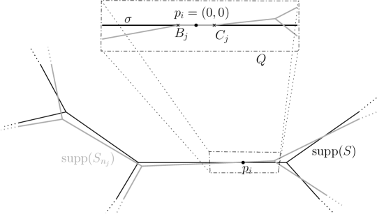
Figure 2. Illustration of our choice of $Q$.

The choice of $Q$ is illustrated in Figure 2. By Lemma 4.2, for this $\rho$, we may choose $j$ large enough such that

$$\mathrm{supp}(S_{n_{j}})\cap\bar{Q}\subset B_{\rho}(\sigma).$$ (4.8)

For $x\in\mathbb{R}$ we denoting by $S_{n_{j}}^{x}$ the slice of $S_{n_{j}}\mathchoice{\mathbin{\vrule width=0.51663pt,height=5.16663pt,depth=0.12915pt\vrule width=3.44444pt,height=0.38748pt,depth=0.12915pt}}{\mathbin{\vrule width=0.51663pt,height=5.16663pt,depth=0.12915pt\vrule width=3.44444pt,height=0.38748pt,depth=0.12915pt}}{\mathbin{\hskip 0.6458pt\vrule width=0.38748pt,height=3.61664pt,depth=0.08612pt\vrule width=2.41109pt,height=0.3014pt,depth=0.08612pt}\hskip 0.6458pt}{\mathbin{\vrule width=0.3014pt,height=2.58334pt,depth=0.04303pt\vrule width=1.72218pt,height=0.25832pt,depth=0.04303pt}}Q$ at the point $x$ with respect to the projection $\pi:\mathbb{R}\times\mathbb{R}^{d-1}\to\mathbb{R}$, see [30, §28] or [19, §4.3]. We infer from the flat convergence of $S_{n_{j}}$ to $S$ that for $\mathscr{H}^{1}$-a.e. $x\in[-8,8]$ it holds

$$\mathbb{F}_{K}(S_{n_{j}}^{x}-\theta\delta_{(x,0)})\to 0\quad\mbox{as $j\to\infty$}$$ (4.9)

and moreover by Lemma 3.2 the multiplicities of $S_{n_{j}}^{x}$ are integer multiples of $k^{-1}$.

We aim to prove that for $j$ sufficiently large there are points $y_{j}^{\pm}\in B^{d-1}_{\rho}(0)$ such that

$$S_{n_{j}}^{\pm 4}=\theta\delta_{(\pm 4,y_{j}^{\pm})},$$ (4.10)

To this aim we seek points $x_{1}(j)\in[-6,-5]$, $x_{2}(j)\in[-2,-1]$, $x_{3}(j)\in[1,2]$ and $x_{4}(j)\in[5,6]$ such that for $i=1,\dots,4$ it holds

$$S_{n_{j}}^{x_{i}(j)}=\theta\delta_{(x_{i}(j),y_{i}(j))},$$ (4.11)

for some points $y_{i}(j)\in B^{d-1}_{\rho}(0)$. If so, by [30, Lemma 28.5], (4.11) and (4.8) imply, denoting

$$Q_{1}^{j}:=(x_{1}(j),x_{2}(j))\times B_{\rho}^{d-1}(0)\quad\mbox{and}\quad Q_{2}^{j}:=(x_{3}(j),x_{4}(j))\times B_{\rho}^{d-1}(0),$$

that

$$\partial(S_{n_{j}}\mathchoice{\mathbin{\vrule width=0.51663pt,height=5.16663pt,depth=0.12915pt\vrule width=3.44444pt,height=0.38748pt,depth=0.12915pt}}{\mathbin{\vrule width=0.51663pt,height=5.16663pt,depth=0.12915pt\vrule width=3.44444pt,height=0.38748pt,depth=0.12915pt}}{\mathbin{\hskip 0.6458pt\vrule width=0.38748pt,height=3.61664pt,depth=0.08612pt\vrule width=2.41109pt,height=0.3014pt,depth=0.08612pt}\hskip 0.6458pt}{\mathbin{\vrule width=0.3014pt,height=2.58334pt,depth=0.04303pt\vrule width=1.72218pt,height=0.25832pt,depth=0.04303pt}}Q_{1}^{j})=S_{n_{j}}^{x_{2}(j)}-S_{n_{j}}^{x_{1}(j)}\quad\mbox{and}\quad\partial(S_{n_{j}}\mathchoice{\mathbin{\vrule width=0.51663pt,height=5.16663pt,depth=0.12915pt\vrule width=3.44444pt,height=0.38748pt,depth=0.12915pt}}{\mathbin{\vrule width=0.51663pt,height=5.16663pt,depth=0.12915pt\vrule width=3.44444pt,height=0.38748pt,depth=0.12915pt}}{\mathbin{\hskip 0.6458pt\vrule width=0.38748pt,height=3.61664pt,depth=0.08612pt\vrule width=2.41109pt,height=0.3014pt,depth=0.08612pt}\hskip 0.6458pt}{\mathbin{\vrule width=0.3014pt,height=2.58334pt,depth=0.04303pt\vrule width=1.72218pt,height=0.25832pt,depth=0.04303pt}}Q_{2}^{j})=S_{n_{j}}^{x_{4}(j)}-S_{n_{j}}^{x_{3}(j)}.$$

In turn, by [2, Proposition 7.4] the latter implies (4.10).

In order to prove (4.11), we focus on the interval $I:=[1,2]$ as the argument for the remaining intervals is identical. Firstly, we observe that by (4.9) we have

$$\liminf_{j}(\mathbb{M}(S_{n_{j}}^{x}))\geq\theta\quad\mbox{for $\mathscr{H}^{1}$-a.e. $x\in I$}.$$ (4.12)

Next, denoting $\Omega:=I\times B_{\rho}^{d-1}(0)$, we claim that for $j$ sufficiently large and for every $C>0$ it holds that

$$\mathscr{H}^{1}(\{x\in I:\mathbb{M}^{\alpha}(S_{n_{j}}^{x})\leq\theta^{\alpha}+C\})>0,$$ (4.13)

where for a 0-current $Z:=\sum_{\ell\in\mathbb{N}}\theta_{\ell}\delta_{z_{\ell}}$ we denoted $\mathbb{M}^{\alpha}(Z):=\sum_{\ell\in\mathbb{N}}|\theta_{\ell}|^{\alpha}$.

Assume by contradiction that (4.13) is false for infinitely many indices $j$. By [14, equation (3.11)], for those indices we have

$$\mathbb{M}^{\alpha}(S_{n_{j}}\mathchoice{\mathbin{\vrule width=0.51663pt,height=5.16663pt,depth=0.12915pt\vrule width=3.44444pt,height=0.38748pt,depth=0.12915pt}}{\mathbin{\vrule width=0.51663pt,height=5.16663pt,depth=0.12915pt\vrule width=3.44444pt,height=0.38748pt,depth=0.12915pt}}{\mathbin{\hskip 0.6458pt\vrule width=0.38748pt,height=3.61664pt,depth=0.08612pt\vrule width=2.41109pt,height=0.3014pt,depth=0.08612pt}\hskip 0.6458pt}{\mathbin{\vrule width=0.3014pt,height=2.58334pt,depth=0.04303pt\vrule width=1.72218pt,height=0.25832pt,depth=0.04303pt}}\bar{\Omega})\geq\theta^{\alpha}+C=\mathbb{M}^{\alpha}(S\mathchoice{\mathbin{\vrule width=0.51663pt,height=5.16663pt,depth=0.12915pt\vrule width=3.44444pt,height=0.38748pt,depth=0.12915pt}}{\mathbin{\vrule width=0.51663pt,height=5.16663pt,depth=0.12915pt\vrule width=3.44444pt,height=0.38748pt,depth=0.12915pt}}{\mathbin{\hskip 0.6458pt\vrule width=0.38748pt,height=3.61664pt,depth=0.08612pt\vrule width=2.41109pt,height=0.3014pt,depth=0.08612pt}\hskip 0.6458pt}{\mathbin{\vrule width=0.3014pt,height=2.58334pt,depth=0.04303pt\vrule width=1.72218pt,height=0.25832pt,depth=0.04303pt}}\bar{\Omega})+C.$$ (4.14)

The latter, combined with (4.4), implies that for the same indices we have

$$\mathbb{M}^{\alpha}(S_{n_{j}}\mathchoice{\mathbin{\vrule width=0.51663pt,height=5.16663pt,depth=0.12915pt\vrule width=3.44444pt,height=0.38748pt,depth=0.12915pt}}{\mathbin{\vrule width=0.51663pt,height=5.16663pt,depth=0.12915pt\vrule width=3.44444pt,height=0.38748pt,depth=0.12915pt}}{\mathbin{\hskip 0.6458pt\vrule width=0.38748pt,height=3.61664pt,depth=0.08612pt\vrule width=2.41109pt,height=0.3014pt,depth=0.08612pt}\hskip 0.6458pt}{\mathbin{\vrule width=0.3014pt,height=2.58334pt,depth=0.04303pt\vrule width=1.72218pt,height=0.25832pt,depth=0.04303pt}}(\mathbb{R}^{d}\setminus\bar{\Omega}))<\mathbb{M}^{\alpha}(S\mathchoice{\mathbin{\vrule width=0.51663pt,height=5.16663pt,depth=0.12915pt\vrule width=3.44444pt,height=0.38748pt,depth=0.12915pt}}{\mathbin{\vrule width=0.51663pt,height=5.16663pt,depth=0.12915pt\vrule width=3.44444pt,height=0.38748pt,depth=0.12915pt}}{\mathbin{\hskip 0.6458pt\vrule width=0.38748pt,height=3.61664pt,depth=0.08612pt\vrule width=2.41109pt,height=0.3014pt,depth=0.08612pt}\hskip 0.6458pt}{\mathbin{\vrule width=0.3014pt,height=2.58334pt,depth=0.04303pt\vrule width=1.72218pt,height=0.25832pt,depth=0.04303pt}}(\mathbb{R}^{d}\setminus\bar{\Omega}))-C,$$

which contradicts [16, Proposition 2.6]. From (4.12) and (4.13) we deduce that for $j$ sufficiently large there exists $x_{1}(j)\in I$ such that

$$\mathbb{M}(S_{n_{j}}^{x_{1}(j)})\geq\theta\quad\mbox{and}\quad\mathbb{M}^{\alpha}(S_{n_{j}}^{x_{1}(j)})\leq\theta^{\alpha}+C.$$ (4.15)

Lastly we prove that if $C$ is sufficiently small, then (4.15) implies

$$S_{n_{j}}^{x_{1}(j)}=\theta\delta_{(x_{1}(j),y_{1}(j))},$$ (4.16)

for some points $y_{1}(j)\in B^{d-1}_{\rho}(0)$, thus completing the proof of (4.11).

Towards a proof by contradiction of (4.16), observe that for every 0-current $Z=\sum_{\ell=1}^{M}\theta_{\ell}\delta_{z_{\ell}}$, with $M\geq 2$, $|\theta_{\ell}|\geq k^{-1}$ and $z_{\ell}$ distinct, satisfying $\mathbb{M}(Z)=\sum_{\ell}|\theta_{\ell}|\geq\theta$, the strict subadditivity of the function $t\mapsto t^{\alpha}$ (for $t>0$) yields the existence of a $\bar{C}=\bar{C}(\alpha,\theta,k)>0$ such that

$$\mathbb{M}^{\alpha}(Z)=|\theta_{1}|^{\alpha}+\sum_{\ell=2}^{M}|\theta_{\ell}|^{\alpha}\geq\min\{(mk^{-1})^{\alpha}+(\theta-mk^{-1})^{\alpha}:m=1,\dots,k\theta-1\}>\theta^{\alpha}+\bar{C}.$$

This contradicts (4.15), by the arbitrariness of $C$.

It follows from (4.10) and [30, Lemma 28.5] that, denoting

$$Q^{\prime}:=(-4,4)\times B_{\rho}^{d-1}(0),\quad A_{j}:=(-4,y_{j}^{-}),\quad D_{j}:=(4,y_{j}^{+}),$$

we have

$$\partial(S_{n_{j}}\mathchoice{\mathbin{\vrule width=0.51663pt,height=5.16663pt,depth=0.12915pt\vrule width=3.44444pt,height=0.38748pt,depth=0.12915pt}}{\mathbin{\vrule width=0.51663pt,height=5.16663pt,depth=0.12915pt\vrule width=3.44444pt,height=0.38748pt,depth=0.12915pt}}{\mathbin{\hskip 0.6458pt\vrule width=0.38748pt,height=3.61664pt,depth=0.08612pt\vrule width=2.41109pt,height=0.3014pt,depth=0.08612pt}\hskip 0.6458pt}{\mathbin{\vrule width=0.3014pt,height=2.58334pt,depth=0.04303pt\vrule width=1.72218pt,height=0.25832pt,depth=0.04303pt}}Q^{\prime})=\theta\left(\delta_{D_{j}}-\delta_{A_{j}}+k^{-1}\big{(}\delta_{B_{j}}-\delta_{C_{j}}\big{)}\right),$$ (4.17)

for $j$ sufficiently large (see Figure 3).

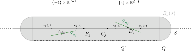
Figure 3. Representation of parts of $S_{n_{j}}\mathchoice{\mathbin{\vrule width=0.51663pt,height=5.16663pt,depth=0.12915pt\vrule width=3.44444pt,height=0.38748pt,depth=0.12915pt}}{\mathbin{\vrule width=0.51663pt,height=5.16663pt,depth=0.12915pt\vrule width=3.44444pt,height=0.38748pt,depth=0.12915pt}}{\mathbin{\hskip 0.6458pt\vrule width=0.38748pt,height=3.61664pt,depth=0.08612pt\vrule width=2.41109pt,height=0.3014pt,depth=0.08612pt}\hskip 0.6458pt}{\mathbin{\vrule width=0.3014pt,height=2.58334pt,depth=0.04303pt\vrule width=1.72218pt,height=0.25832pt,depth=0.04303pt}}Q$.

4.3. Analysis of the possible topologies of $S_{n_{j}}\mathchoice{\mathbin{\vrule width=0.51663pt,height=5.16663pt,depth=0.12915pt\vrule width=3.44444pt,height=0.38748pt,depth=0.12915pt}}{\mathbin{\vrule width=0.51663pt,height=5.16663pt,depth=0.12915pt\vrule width=3.44444pt,height=0.38748pt,depth=0.12915pt}}{\mathbin{\hskip 0.6458pt\vrule width=0.38748pt,height=3.61664pt,depth=0.08612pt\vrule width=2.41109pt,height=0.3014pt,depth=0.08612pt}\hskip 0.6458pt}{\mathbin{\vrule width=0.3014pt,height=2.58334pt,depth=0.04303pt\vrule width=1.72218pt,height=0.25832pt,depth=0.04303pt}}Q^{\prime}$.

Since $S_{n_{j}}\in\textbf{OTP}(b_{n_{j}})$ we must have $S_{n_{j}}\mathchoice{\mathbin{\vrule width=0.51663pt,height=5.16663pt,depth=0.12915pt\vrule width=3.44444pt,height=0.38748pt,depth=0.12915pt}}{\mathbin{\vrule width=0.51663pt,height=5.16663pt,depth=0.12915pt\vrule width=3.44444pt,height=0.38748pt,depth=0.12915pt}}{\mathbin{\hskip 0.6458pt\vrule width=0.38748pt,height=3.61664pt,depth=0.08612pt\vrule width=2.41109pt,height=0.3014pt,depth=0.08612pt}\hskip 0.6458pt}{\mathbin{\vrule width=0.3014pt,height=2.58334pt,depth=0.04303pt\vrule width=1.72218pt,height=0.25832pt,depth=0.04303pt}}Q^{\prime}\in\textbf{OTP}(\partial(S_{n_{j}}\mathchoice{\mathbin{\vrule width=0.51663pt,height=5.16663pt,depth=0.12915pt\vrule width=3.44444pt,height=0.38748pt,depth=0.12915pt}}{\mathbin{\vrule width=0.51663pt,height=5.16663pt,depth=0.12915pt\vrule width=3.44444pt,height=0.38748pt,depth=0.12915pt}}{\mathbin{\hskip 0.6458pt\vrule width=0.38748pt,height=3.61664pt,depth=0.08612pt\vrule width=2.41109pt,height=0.3014pt,depth=0.08612pt}\hskip 0.6458pt}{\mathbin{\vrule width=0.3014pt,height=2.58334pt,depth=0.04303pt\vrule width=1.72218pt,height=0.25832pt,depth=0.04303pt}}Q^{\prime}))$. In general, we will denote by $\sigma_{PR}$ the oriented segment from the point $P$ to the point $R$. We aim to prove that for $k\geq k_{0}(\alpha)$ and for $\rho\leq\rho(k)$ sufficiently small it holds $S_{n_{j}}\mathchoice{\mathbin{\vrule width=0.51663pt,height=5.16663pt,depth=0.12915pt\vrule width=3.44444pt,height=0.38748pt,depth=0.12915pt}}{\mathbin{\vrule width=0.51663pt,height=5.16663pt,depth=0.12915pt\vrule width=3.44444pt,height=0.38748pt,depth=0.12915pt}}{\mathbin{\hskip 0.6458pt\vrule width=0.38748pt,height=3.61664pt,depth=0.08612pt\vrule width=2.41109pt,height=0.3014pt,depth=0.08612pt}\hskip 0.6458pt}{\mathbin{\vrule width=0.3014pt,height=2.58334pt,depth=0.04303pt\vrule width=1.72218pt,height=0.25832pt,depth=0.04303pt}}Q^{\prime}\in\{W_{j},Z_{j}\}$, for $j$ large enough, where

$$W_{j}:=\theta\left(\llbracket\sigma_{A_{j}B_{j}}\rrbracket+\llbracket\sigma_{C_{j}D_{j}}\rrbracket+\frac{k-1}{k}\llbracket\sigma_{B_{j}C_{j}}\rrbracket\right)\quad\mbox{and}\quad Z_{j}:=\theta\left(\llbracket\sigma_{A_{j}D_{j}}\rrbracket+\frac{1}{k}\llbracket\sigma_{C_{j}B_{j}}\rrbracket\right)\,,$$ (4.18)

see Table LABEL:FigONES. We will do this by excluding every other topology comparing angle conditions which are given by the multiplicities of the segments (which depend on $k$) and contradict the choice of $\rho$. Thus, when we say for $\rho$ small enough, we mean implicitly to choose $j$ large enough such that by Lemma 4.2, we have $\mathrm{supp}(S_{n_{j}})\subset B_{\rho}(\mathrm{supp}(S)\cup\{p_{1},\dots,p_{h}\})$ for the desired $\rho$ .

Write $S_{n_{j}}\mathchoice{\mathbin{\vrule width=0.51663pt,height=5.16663pt,depth=0.12915pt\vrule width=3.44444pt,height=0.38748pt,depth=0.12915pt}}{\mathbin{\vrule width=0.51663pt,height=5.16663pt,depth=0.12915pt\vrule width=3.44444pt,height=0.38748pt,depth=0.12915pt}}{\mathbin{\hskip 0.6458pt\vrule width=0.38748pt,height=3.61664pt,depth=0.08612pt\vrule width=2.41109pt,height=0.3014pt,depth=0.08612pt}\hskip 0.6458pt}{\mathbin{\vrule width=0.3014pt,height=2.58334pt,depth=0.04303pt\vrule width=1.72218pt,height=0.25832pt,depth=0.04303pt}}Q^{\prime}=\sum_{i<j}a_{ij}\llbracket\sigma_{ij}\rrbracket$ as in (3.8) and observe that by Lemma 3.4, as $\mathscr{H}^{0}(\partial(S_{n_{j}}\mathchoice{\mathbin{\vrule width=0.51663pt,height=5.16663pt,depth=0.12915pt\vrule width=3.44444pt,height=0.38748pt,depth=0.12915pt}}{\mathbin{\vrule width=0.51663pt,height=5.16663pt,depth=0.12915pt\vrule width=3.44444pt,height=0.38748pt,depth=0.12915pt}}{\mathbin{\hskip 0.6458pt\vrule width=0.38748pt,height=3.61664pt,depth=0.08612pt\vrule width=2.41109pt,height=0.3014pt,depth=0.08612pt}\hskip 0.6458pt}{\mathbin{\vrule width=0.3014pt,height=2.58334pt,depth=0.04303pt\vrule width=1.72218pt,height=0.25832pt,depth=0.04303pt}}Q^{\prime}))=4$, then $\mathscr{H}^{0}(\textbf{BR}(S_{n_{j}}\mathchoice{\mathbin{\vrule width=0.51663pt,height=5.16663pt,depth=0.12915pt\vrule width=3.44444pt,height=0.38748pt,depth=0.12915pt}}{\mathbin{\vrule width=0.51663pt,height=5.16663pt,depth=0.12915pt\vrule width=3.44444pt,height=0.38748pt,depth=0.12915pt}}{\mathbin{\hskip 0.6458pt\vrule width=0.38748pt,height=3.61664pt,depth=0.08612pt\vrule width=2.41109pt,height=0.3014pt,depth=0.08612pt}\hskip 0.6458pt}{\mathbin{\vrule width=0.3014pt,height=2.58334pt,depth=0.04303pt\vrule width=1.72218pt,height=0.25832pt,depth=0.04303pt}}Q^{\prime}))\in\{0,1,2\}$. We thus analyze the three cases separately and we recall that, by Lemma 3.6, in order to prove (4.18) it suffices to prove that

$$\mathrm{supp}(S_{n_{j}}\mathchoice{\mathbin{\vrule width=0.51663pt,height=5.16663pt,depth=0.12915pt\vrule width=3.44444pt,height=0.38748pt,depth=0.12915pt}}{\mathbin{\vrule width=0.51663pt,height=5.16663pt,depth=0.12915pt\vrule width=3.44444pt,height=0.38748pt,depth=0.12915pt}}{\mathbin{\hskip 0.6458pt\vrule width=0.38748pt,height=3.61664pt,depth=0.08612pt\vrule width=2.41109pt,height=0.3014pt,depth=0.08612pt}\hskip 0.6458pt}{\mathbin{\vrule width=0.3014pt,height=2.58334pt,depth=0.04303pt\vrule width=1.72218pt,height=0.25832pt,depth=0.04303pt}}Q^{\prime})=\sigma_{A_{j}B_{j}}\cup\sigma_{B_{j}C_{j}}\cup\sigma_{C_{j}D_{j}}\quad\mbox{or}\quad\mathrm{supp}(S_{n_{j}}\mathchoice{\mathbin{\vrule width=0.51663pt,height=5.16663pt,depth=0.12915pt\vrule width=3.44444pt,height=0.38748pt,depth=0.12915pt}}{\mathbin{\vrule width=0.51663pt,height=5.16663pt,depth=0.12915pt\vrule width=3.44444pt,height=0.38748pt,depth=0.12915pt}}{\mathbin{\hskip 0.6458pt\vrule width=0.38748pt,height=3.61664pt,depth=0.08612pt\vrule width=2.41109pt,height=0.3014pt,depth=0.08612pt}\hskip 0.6458pt}{\mathbin{\vrule width=0.3014pt,height=2.58334pt,depth=0.04303pt\vrule width=1.72218pt,height=0.25832pt,depth=0.04303pt}}Q^{\prime})=\sigma_{A_{j}D_{j}}\cup\sigma_{B_{j}C_{j}}.$$

Table 1. Representation of $W_{j}$ and $Z_{j}$. From now on $\delta:=\theta/k$ and we remove the subscript $j$ from the points.

$W_{j}$
$Z_{j}$

Case 1: $\textbf{BR}(S_{n_{j}}\mathchoice{\mathbin{\vrule width=0.51663pt,height=5.16663pt,depth=0.12915pt\vrule width=3.44444pt,height=0.38748pt,depth=0.12915pt}}{\mathbin{\vrule width=0.51663pt,height=5.16663pt,depth=0.12915pt\vrule width=3.44444pt,height=0.38748pt,depth=0.12915pt}}{\mathbin{\hskip 0.6458pt\vrule width=0.38748pt,height=3.61664pt,depth=0.08612pt\vrule width=2.41109pt,height=0.3014pt,depth=0.08612pt}\hskip 0.6458pt}{\mathbin{\vrule width=0.3014pt,height=2.58334pt,depth=0.04303pt\vrule width=1.72218pt,height=0.25832pt,depth=0.04303pt}}Q^{\prime})=\emptyset$. Recalling [2, Proposition 7.4], $\mathrm{supp}(S_{n_{j}}\mathchoice{\mathbin{\vrule width=0.51663pt,height=5.16663pt,depth=0.12915pt\vrule width=3.44444pt,height=0.38748pt,depth=0.12915pt}}{\mathbin{\vrule width=0.51663pt,height=5.16663pt,depth=0.12915pt\vrule width=3.44444pt,height=0.38748pt,depth=0.12915pt}}{\mathbin{\hskip 0.6458pt\vrule width=0.38748pt,height=3.61664pt,depth=0.08612pt\vrule width=2.41109pt,height=0.3014pt,depth=0.08612pt}\hskip 0.6458pt}{\mathbin{\vrule width=0.3014pt,height=2.58334pt,depth=0.04303pt\vrule width=1.72218pt,height=0.25832pt,depth=0.04303pt}}Q^{\prime})$ must be one of the following sets, sorted alphabetically:

• $\sigma_{A_{j}B_{j}}\cup\sigma_{A_{j}C_{j}}\cup\sigma_{A_{j}D_{j}}$,

• $\sigma_{A_{j}B_{j}}\cup\sigma_{A_{j}C_{j}}\cup\sigma_{B_{j}D_{j}}$,

• $\sigma_{A_{j}B_{j}}\cup\sigma_{A_{j}C_{j}}\cup\sigma_{C_{j}D_{j}}$,

• $\sigma_{A_{j}B_{j}}\cup\sigma_{A_{j}D_{j}}\cup\sigma_{B_{j}C_{j}}$,

• $\sigma_{A_{j}B_{j}}\cup\sigma_{A_{j}D_{j}}\cup\sigma_{C_{j}D_{j}}$,

• $\sigma_{A_{j}B_{j}}\cup\sigma_{B_{j}C_{j}}\cup\sigma_{B_{j}D_{j}}$,

• $\sigma_{A_{j}B_{j}}\cup\sigma_{B_{j}C_{j}}\cup\sigma_{C_{j}D_{j}}$,

• $\sigma_{A_{j}B_{j}}\cup\sigma_{B_{j}D_{j}}\cup\sigma_{C_{j}D_{j}}$,

• $\sigma_{A_{j}B_{j}}\cup\sigma_{C_{j}D_{j}}$,

• $\sigma_{A_{j}C_{j}}\cup\sigma_{A_{j}D_{j}}\cup\sigma_{B_{j}C_{j}}$,

• $\sigma_{A_{j}C_{j}}\cup\sigma_{A_{j}D_{j}}\cup\sigma_{B_{j}D_{j}}$,

• $\sigma_{A_{j}C_{j}}\cup\sigma_{B_{j}C_{j}}\cup\sigma_{B_{j}D_{j}}$,

• $\sigma_{A_{j}C_{j}}\cup\sigma_{B_{j}C_{j}}\cup\sigma_{C_{j}D_{j}}$,

• $\sigma_{A_{j}C_{j}}\cup\sigma_{B_{j}D_{j}}$,

• $\sigma_{A_{j}C_{j}}\cup\sigma_{B_{j}D_{j}}\cup\sigma_{C_{j}D_{j}}$,

• $\sigma_{A_{j}D_{j}}\cup\sigma_{B_{j}C_{j}}$,

• $\sigma_{A_{j}D_{j}}\cup\sigma_{B_{j}C_{j}}\cup\sigma_{B_{j}D_{j}}$,

• $\sigma_{A_{j}D_{j}}\cup\sigma_{B_{j}C_{j}}\cup\sigma_{C_{j}D_{j}}$,

• $\sigma_{A_{j}D_{j}}\cup\sigma_{B_{j}D_{j}}\cup\sigma_{C_{j}D_{j}}$.

Observe that we omitted the cases

• $\sigma_{A_{j}B_{j}}\cup\sigma_{A_{j}C_{j}}\cup\sigma_{B_{j}C_{j}}$,

• $\sigma_{A_{j}B_{j}}\cup\sigma_{A_{j}D_{j}}\cup\sigma_{B_{j}D_{j}}$,

• $\sigma_{A_{j}C_{j}}\cup\sigma_{A_{j}D_{j}}\cup\sigma_{C_{j}D_{j}}$

• $\sigma_{B_{j}C_{j}}\cup\sigma_{B_{j}D_{j}}\cup\sigma_{C_{j}D_{j}}$

because, independently of the position of the points, the support either contains a loop or does not contain one of the four points in the support of the boundary. The only exceptions to this behaviour are (ii) and (iii) only when the four points are collinear, which is not relevant, as we discuss in Sub-case 1-1 below.

Sub-case 1-1. Firstly we observe that when the points $A_{j},B_{j},C_{j},D_{j}$ are collinear the only admissible competitor is $Z_{j}$.

Sub-case 1-2. Next, we analyze the case in which no triples among the points $A_{j},B_{j},C_{j},D_{j}$ are contained in a line.

We immediately exclude those cases for which the corresponding set is not the support of any current with boundary $\partial(S_{n_{j}}\mathchoice{\mathbin{\vrule width=0.51663pt,height=5.16663pt,depth=0.12915pt\vrule width=3.44444pt,height=0.38748pt,depth=0.12915pt}}{\mathbin{\vrule width=0.51663pt,height=5.16663pt,depth=0.12915pt\vrule width=3.44444pt,height=0.38748pt,depth=0.12915pt}}{\mathbin{\hskip 0.6458pt\vrule width=0.38748pt,height=3.61664pt,depth=0.08612pt\vrule width=2.41109pt,height=0.3014pt,depth=0.08612pt}\hskip 0.6458pt}{\mathbin{\vrule width=0.3014pt,height=2.58334pt,depth=0.04303pt\vrule width=1.72218pt,height=0.25832pt,depth=0.04303pt}}Q^{\prime})$. Hence we can exclude (1i) and (1n), because the endpoints of the two segments in the support have different multiplicities. Moreover we exclude (1d), (1j), (1q) and (1r) as well, because the segment $\sigma_{A_{j},D_{j}}$ should have multiplicity $\theta$, being either for $A_{j}$ or $D_{j}$ the only segment in the support containing it. On the other hand, the remaining point (respectively $D_{j}$ or $A_{j}$) is an endpoint also for a different segment of the support, from which we deduce that the multiplicity of the latter segment should be 0 (see Table LABEL:Fig1).

Table 2. Representation of (1d), (1i), (1j), (1n), (1q), (1r).

1d	1i
1j	1n
1q	1r

We exclude the following cases by direct comparison with the $\alpha$-mass of $Z_{j}$, for $j$ sufficiently large (see Table LABEL:Fig2):

• (1a), whose corresponding $\alpha$-mass is

  $$\theta^{\alpha}(\mathscr{H}^{1}(\sigma_{A_{j}D_{j}})+k^{-\alpha}(\mathscr{H}^{1}(\sigma_{A_{j}B_{j}})+\mathscr{H}^{1}(\sigma_{A_{j}C_{j}}))>\mathbb{M}^{\alpha}(Z_{j}).$$

• (1b), whose corresponding $\alpha$-mass is

  $$\theta^{\alpha}((1+k^{-1})^{\alpha}\mathscr{H}^{1}(\sigma_{A_{j}B_{j}})+\mathscr{H}^{1}(\sigma_{B_{j}D_{j}})+k^{-\alpha}\mathscr{H}^{1}(\sigma_{A_{j}C_{j}}))>\mathbb{M}^{\alpha}(Z_{j}).$$

• (1f), whose corresponding $\alpha$-mass is

  $$\theta^{\alpha}(\mathscr{H}^{1}(\sigma_{A_{j}B_{j}})+\mathscr{H}^{1}(\sigma_{B_{j}D_{j}})+k^{-\alpha}\mathscr{H}^{1}(\sigma_{B_{j}C_{j}}))>\mathbb{M}^{\alpha}(Z_{j}).$$

• (1k), whose corresponding $\alpha$-mass is

  $$\theta^{\alpha}((1+k^{-1})^{\alpha}\mathscr{H}^{1}(\sigma_{A_{j}D_{j}})+k^{-\alpha}(\mathscr{H}^{1}(\sigma_{A_{j}C_{j}})+\mathscr{H}^{1}(\sigma_{B_{j}D_{j}})))>\mathbb{M}^{\alpha}(Z_{j}).$$

• (1l), whose corresponding $\alpha$-mass is

  $$\theta^{\alpha}((1+k^{-1})^{\alpha}\mathscr{H}^{1}(\sigma_{B_{j}C_{j}})+\mathscr{H}^{1}(\sigma_{A_{j}C_{j}})+\mathscr{H}^{1}(\sigma_{B_{j}D_{j}}))>\mathbb{M}^{\alpha}(Z_{j}).$$

• (1m), whose corresponding $\alpha$-mass is

  $$\theta^{\alpha}(\mathscr{H}^{1}(\sigma_{A_{j}C_{j}})+\mathscr{H}^{1}(\sigma_{C_{j}D_{j}})+k^{-\alpha}\mathscr{H}^{1}(\sigma_{B_{j}C_{j}}))>\mathbb{M}^{\alpha}(Z_{j}).$$

• (1o), whose corresponding $\alpha$-mass is

  $$\theta^{\alpha}((1+k^{-1})^{\alpha}\mathscr{H}^{1}(\sigma_{C_{j}D_{j}})+\mathscr{H}^{1}(\sigma_{A_{j}C_{j}})+k^{-\alpha}\mathscr{H}^{1}(\sigma_{B_{j}D_{j}}))>\mathbb{M}^{\alpha}(Z_{j}).$$

• (1s), whose corresponding $\alpha$-mass is

  $$\theta^{\alpha}(\mathscr{H}^{1}(\sigma_{A_{j}D_{j}})+k^{-\alpha}(\mathscr{H}^{1}(\sigma_{B_{j}D_{j}})+\mathscr{H}^{1}(\sigma_{C_{j}D_{j}}))>\mathbb{M}^{\alpha}(Z_{j}).$$

Table 3. Representation of (1a), (1b), (1f), (1k), (1l), (1m), (1o), (1s).

1a
1b
1f
1k
1l
1m
1o
1s

For $j$ sufficiently large and for $k\geq k_{0}(\alpha)$, the $\alpha$-mass corresponding to (1c) is (see Table LABEL:Figch)

$$\begin{split}&\theta^{\alpha}(\mathscr{H}^{1}(\sigma_{C_{j}D_{j}})+(1-k^{-1})^{\alpha}\mathscr{H}^{1}(\sigma_{A_{j}C_{j}})+k^{-\alpha}\mathscr{H}^{1}(\sigma_{A_{j}B_{j}}))\\ &>\theta^{\alpha}(\mathscr{H}^{1}(\sigma_{C_{j}D_{j}})+((1-k^{-1})^{\alpha}+k^{-\alpha})\mathscr{H}^{1}(\sigma_{A_{j}B_{j}}))\\ &>\theta^{\alpha}(\mathscr{H}^{1}(\sigma_{C_{j}D_{j}})+\mathscr{H}^{1}(\sigma_{A_{j}B_{j}})+\frac{k^{-\alpha}}{2}\mathscr{H}^{1}(\sigma_{A_{j}B_{j}}))\\ &>\theta^{\alpha}(\mathscr{H}^{1}(\sigma_{C_{j}D_{j}})+\mathscr{H}^{1}(\sigma_{A_{j}B_{j}})+k^{-\alpha}\mathscr{H}^{1}(\sigma_{B_{j}C_{j}}))=\mathbb{M}^{\alpha}(W_{j}).\end{split}$$ (4.19)

Also, for $j$ sufficiently large and for $k\geq k_{0}(\alpha)$, the $\alpha$-mass corresponding to (1h) is (see Table LABEL:Figch)

$$\begin{split}&\theta^{\alpha}(\mathscr{H}^{1}(\sigma_{A_{j}B_{j}})+(1-k^{-1})^{\alpha}\mathscr{H}^{1}(\sigma_{B_{j}D_{j}})+k^{-\alpha}\mathscr{H}^{1}(\sigma_{C_{j}D_{j}}))\\ &>\theta^{\alpha}(\mathscr{H}^{1}(\sigma_{A_{j}B_{j}})+((1-k^{-1})^{\alpha}+k^{-\alpha})\mathscr{H}^{1}(\sigma_{C_{j}D_{j}}))\\ &>\theta^{\alpha}(\mathscr{H}^{1}(\sigma_{A_{j}B_{j}})+\mathscr{H}^{1}(\sigma_{C_{j}D_{j}})+\frac{k^{-\alpha}}{2}\mathscr{H}^{1}(\sigma_{C_{j}D_{j}}))\\ &>\theta^{\alpha}(\mathscr{H}^{1}(\sigma_{A_{j}B_{j}})+\mathscr{H}^{1}(\sigma_{C_{j}D_{j}})+k^{-\alpha}\mathscr{H}^{1}(\sigma_{B_{j}C_{j}}))=\mathbb{M}^{\alpha}(W_{j}).\end{split}$$ (4.20)

Table 4. Representation of (1c), (1h).

1c
1h

Lastly, we exclude case (1e) by direct comparison with the $\alpha$-mass of $Z_{j}$. For $j$ sufficiently large and for $k\geq k_{0}(\alpha)$, the $\alpha$-mass corresponding to (1e) is (see Table LABEL:Fige)

$$\begin{split}&\theta^{\alpha}((1-k^{-1})^{\alpha}\mathscr{H}^{1}(\sigma_{A_{j}D_{j}})+k^{-\alpha}(\mathscr{H}^{1}(\sigma_{A_{j}B_{j}})+\mathscr{H}^{1}(\sigma_{C_{j}D_{j}})))\\ &>\theta^{\alpha}((1-k^{-1})^{\alpha}\mathscr{H}^{1}(\sigma_{A_{j}D_{j}})+k^{-\alpha}\frac{1}{2}\mathscr{H}^{1}(\sigma_{A_{j}D_{j}}))\\ &>\theta^{\alpha}(\mathscr{H}^{1}(\sigma_{A_{j}D_{j}})+\frac{1}{4}k^{-\alpha}\mathscr{H}^{1}(\sigma_{A_{j}D_{j}}))\\ &>\theta^{\alpha}(\mathscr{H}^{1}(\sigma_{A_{j}D_{j}})+k^{-\alpha}\mathscr{H}^{1}(\sigma_{B_{j}C_{j}}))=\mathbb{M}^{\alpha}(Z_{j}).\end{split}$$ (4.21)

Table 5. Representation of (1e).

1e

Sub-case 1-3. The last situation which we need to take into account is when exactly three points are collinear. We will discuss the case in which the collinear points are $A_{j}$, $B_{j}$ and $C_{j}$ or $A_{j},C_{j}$ and $D_{j}$. The remaining cases in which the collinear points are $B_{j}$, $C_{j}$ and $D_{j}$ or $A_{j},B_{j}$ and $D_{j}$ are symmetric and can be treated analogously, therefore we leave the analysis to the reader.

Sub-case 1-3-1: $A_{j}$, $B_{j}$ and $C_{j}$ are collinear.

The cases (1d), (1i), (1j), (1q), (1r) can be excluded for the same reason as in the Sub-case 1-2 (see Table LABEL:Fig_wrong).

We exclude cases (1b), (1f), (1l), (1n), which are coincident (see Table LABEL:Fignall), by direct comparison with the $\alpha$-mass of $Z_{j}$. For $j$ sufficiently large, the $\alpha$-mass corresponding to the above cases is

$$\theta^{\alpha}(\mathscr{H}^{1}(\sigma_{A_{j}B_{j}})+\mathscr{H}^{1}(\sigma_{B_{j}D_{j}})+k^{-\alpha}\mathscr{H}^{1}(\sigma_{B_{j}C_{j}}))>\mathbb{M}^{\alpha}(Z_{j}).$$

Table 6. Representation of (1d), (1i), (1j), (1q), (1r) in the collinear case.

1d	1i
1j	1q
1r

Table 7. Representation of (1b), (1f), (1l), (1n) in the collinear case.

We exclude case (1a), since it coincides with case (1j), which we have already excluded and we exclude cases (1k) and (1o) because they contain a loop (see Table LABEL:Figloop).

Table 8. Representation of (1k) and (1o) in the collinear case.

1k

1o

We do not need to exclude cases (1c) and (1m), since the current coincides with $Z_{j}$ (see Table LABEL:Figcm).

Table 9. Representation of (1c), (1m) in the collinear case.

Lastly, cases (1e), (1h), (1s) can be excluded with the same argument used in Sub-case 1-2, since the segments in the corresponding support are in general position also when $A_{j},B_{j}$, and $C_{j}$ are collinear (see Table LABEL:Fehs).

Table 10. Representation of (1e), (1h), (1s) in the collinear case.

1e	1h
1s

Sub-case 1-3-2: $A_{j}$, $C_{j}$ and $D_{j}$ are collinear.

The cases (1d), (1i), (1n), (1q) can be excluded for the same reason as in the Sub-case 1-2 (see Table LABEL:Fig_wrong2).

Table 11. Representation of (1d), (1i), (1n), (1q) in the collinear case.

1d	1i
1n	1q

We exclude cases (1k), (1o), (1s), which are coincident (see Table LABEL:Fignall2first), by direct comparison with the $\alpha$-mass of $Z_{j}$. For $j$ sufficiently large, the $\alpha$-mass corresponding to the above cases is

$$\theta^{\alpha}((1+k^{-1})^{\alpha}\mathscr{H}^{1}(\sigma_{C_{j}D_{j}})+\mathscr{H}^{1}(\sigma_{A_{j}C_{j}})+k^{-\alpha}\mathscr{H}^{1}(\sigma_{B_{j}D_{j}}))>\mathbb{M}^{\alpha}(Z_{j}).$$

Table 12. Representation of (1k), (1o), (1s) in the collinear case.

We do not exclude cases (1j), (1m) and (1r), since the current coincides with $Z_{j}$ (see Table LABEL:Figcm2).

Table 13. Representation of (1j), (1m), (1r) in the collinear case.

We exclude cases (1a), (1c), (1e), which are coincident (see Table LABEL:Fignall2), by direct comparison with the $\alpha$-mass of $W_{j}$. For $j$ sufficiently large and for $k\geq k_{0}(\alpha)$, the $\alpha$-mass corresponding to the above cases is

$$\begin{split}&\theta^{\alpha}(\mathscr{H}^{1}(\sigma_{C_{j}D_{j}})+(1-k^{-1})^{\alpha}\mathscr{H}^{1}(\sigma_{A_{j}C_{j}})+k^{-\alpha}\mathscr{H}^{1}(\sigma_{A_{j}B_{j}}))\\ &>\theta^{\alpha}(\mathscr{H}^{1}(\sigma_{C_{j}D_{j}})+((1-k^{-1})^{\alpha}+k^{-\alpha})\mathscr{H}^{1}(\sigma_{A_{j}B_{j}}))\\ &>\theta^{\alpha}(\mathscr{H}^{1}(\sigma_{C_{j}D_{j}})+(1+\frac{1}{2}k^{-\alpha})\mathscr{H}^{1}(\sigma_{A_{j}B_{j}}))\\ &>\theta^{\alpha}(\mathscr{H}^{1}(\sigma_{C_{j}D_{j}})+\mathscr{H}^{1}(\sigma_{A_{j}B_{j}})+k^{-\alpha}\mathscr{H}^{1}(\sigma_{B_{j}C_{j}}))=\mathbb{M}^{\alpha}(W_{j}).\end{split}$$ (4.22)

Table 14. Representation of (1a), (1c), (1e) in the collinear case.

Lastly, cases (1b), (1f), (1h), (1l) can be excluded with the same argument used in Sub-case 1-2, since the segments in the corresponding support are in general position also when $A_{j},C_{j}$, and $D_{j}$ are collinear (see Table LABEL:Fehs2).

Table 15. Representation of (1b), (1f), (1h), (1l) in the collinear case.

1b	1f
1h	1l

Case 2: $\textbf{BR}(S_{n_{j}}\mathchoice{\mathbin{\vrule width=0.51663pt,height=5.16663pt,depth=0.12915pt\vrule width=3.44444pt,height=0.38748pt,depth=0.12915pt}}{\mathbin{\vrule width=0.51663pt,height=5.16663pt,depth=0.12915pt\vrule width=3.44444pt,height=0.38748pt,depth=0.12915pt}}{\mathbin{\hskip 0.6458pt\vrule width=0.38748pt,height=3.61664pt,depth=0.08612pt\vrule width=2.41109pt,height=0.3014pt,depth=0.08612pt}\hskip 0.6458pt}{\mathbin{\vrule width=0.3014pt,height=2.58334pt,depth=0.04303pt\vrule width=1.72218pt,height=0.25832pt,depth=0.04303pt}}Q^{\prime})=\{E_{j}\}$. Recalling that $E_{j}$ is the endpoint of at least three segments in the support of $S_{n_{j}}\mathchoice{\mathbin{\vrule width=0.51663pt,height=5.16663pt,depth=0.12915pt\vrule width=3.44444pt,height=0.38748pt,depth=0.12915pt}}{\mathbin{\vrule width=0.51663pt,height=5.16663pt,depth=0.12915pt\vrule width=3.44444pt,height=0.38748pt,depth=0.12915pt}}{\mathbin{\hskip 0.6458pt\vrule width=0.38748pt,height=3.61664pt,depth=0.08612pt\vrule width=2.41109pt,height=0.3014pt,depth=0.08612pt}\hskip 0.6458pt}{\mathbin{\vrule width=0.3014pt,height=2.58334pt,depth=0.04303pt\vrule width=1.72218pt,height=0.25832pt,depth=0.04303pt}}Q^{\prime}$, see the proof of Lemma 3.4, the only possibilities are that $\mathrm{supp}(S_{n_{j}}\mathchoice{\mathbin{\vrule width=0.51663pt,height=5.16663pt,depth=0.12915pt\vrule width=3.44444pt,height=0.38748pt,depth=0.12915pt}}{\mathbin{\vrule width=0.51663pt,height=5.16663pt,depth=0.12915pt\vrule width=3.44444pt,height=0.38748pt,depth=0.12915pt}}{\mathbin{\hskip 0.6458pt\vrule width=0.38748pt,height=3.61664pt,depth=0.08612pt\vrule width=2.41109pt,height=0.3014pt,depth=0.08612pt}\hskip 0.6458pt}{\mathbin{\vrule width=0.3014pt,height=2.58334pt,depth=0.04303pt\vrule width=1.72218pt,height=0.25832pt,depth=0.04303pt}}Q^{\prime})$ is one of the following sets (see Table LABEL:Fig16):

• $\sigma_{A_{j}E_{j}}\cup\sigma_{B_{j}E_{j}}\cup\sigma_{C_{j}E_{j}}\cup\sigma$, with $\sigma\neq\sigma_{D_{j}E_{j}}$,

• $\sigma_{A_{j}E_{j}}\cup\sigma_{B_{j}E_{j}}\cup\sigma_{D_{j}E_{j}}\cup\sigma$, with $\sigma\neq\sigma_{C_{j}E_{j}}$,

• $\sigma_{A_{j}E_{j}}\cup\sigma_{C_{j}E_{j}}\cup\sigma_{D_{j}E_{j}}\cup\sigma$, with $\sigma\neq\sigma_{B_{j}E_{j}}$,

• $\sigma_{B_{j}E_{j}}\cup\sigma_{C_{j}E_{j}}\cup\sigma_{D_{j}E_{j}}\cup\sigma$, with $\sigma\neq\sigma_{A_{j}E_{j}}$,

• $\sigma_{A_{j}E_{j}}\cup\sigma_{B_{j}E_{j}}\cup\sigma_{C_{j}E_{j}}\cup\sigma_{D_{j}E_{j}}$.

We exclude case (2a), indeed by [2, Lemma 12.1 and Lemma 12.2], $E_{j}\in{\rm{conv}}(\{A_{j},B_{j},C_{j}\})$, hence we have for $\rho$ small and $j$ sufficiently large

$$\pi-O(\rho)=\angle{A_{j}B_{j}C_{j}}\leq\angle{A_{j}E_{j}C_{j}}\leq\pi\,.$$ (4.23)

This contradicts [2, Lemma 12.2] for $\rho\leq\rho(k)$, since the modulus of the multiplicity of $\sigma_{A_{j}E_{j}},\sigma_{E_{j}B_{j}}$ and $\sigma_{E_{j}C_{j}}$ belongs to $[k^{-1},\mathbb{M}(b_{n_{j}})]$, which by (4.2) is contained in $[k^{-1},(1+hk^{-1})\mathbb{M}(b)]$.

Cases (2b), (2c) and (2d) are excluded with a similar argument as in case (2a), where the angle $\angle{A_{j}E_{j}C_{j}}$ in (4.23) is replaced respectively by $\angle{A_{j}E_{j}D_{j}}$, $\angle{A_{j}E_{j}D_{j}}$ and $\angle{B_{j}E_{j}D_{j}}$.

We exclude case (2e) by direct comparison with the $\alpha$-mass of $Z_{j}$. The $\alpha$-mass corresponding to (2e) is

$$\begin{split}&\theta^{\alpha}(\mathscr{H}^{1}(\sigma_{A_{j}E_{j}})+\mathscr{H}^{1}(\sigma_{E_{j}D_{j}})+k^{-\alpha}(\mathscr{H}^{1}(\sigma_{B_{j}E_{j}})+\mathscr{H}^{1}(\sigma_{E_{j}C_{j}})))\\ &\geq\theta^{\alpha}(\mathscr{H}^{1}(\sigma_{A_{j}D_{j}})+k^{-\alpha}\mathscr{H}^{1}(\sigma_{B_{j}C_{j}}))=\mathbb{M}^{\alpha}(Z_{j}),\end{split}$$ (4.24)

where the inequality is strict unless $\{E_{j}\}=\sigma_{A_{j}D_{j}}\cap\sigma_{B_{j}C_{j}}$, namely unless the current is $Z_{j}$, which of course we do not need to exclude.

Case 3: $\textbf{BR}(S_{n_{j}}\mathchoice{\mathbin{\vrule width=0.51663pt,height=5.16663pt,depth=0.12915pt\vrule width=3.44444pt,height=0.38748pt,depth=0.12915pt}}{\mathbin{\vrule width=0.51663pt,height=5.16663pt,depth=0.12915pt\vrule width=3.44444pt,height=0.38748pt,depth=0.12915pt}}{\mathbin{\hskip 0.6458pt\vrule width=0.38748pt,height=3.61664pt,depth=0.08612pt\vrule width=2.41109pt,height=0.3014pt,depth=0.08612pt}\hskip 0.6458pt}{\mathbin{\vrule width=0.3014pt,height=2.58334pt,depth=0.04303pt\vrule width=1.72218pt,height=0.25832pt,depth=0.04303pt}}Q^{\prime})=\{E_{j},F_{j}\}$. Recalling [2, Proposition 7.4], and the fact that both $E_{j}$ and $F_{j}$ are the endpoints of at least three segments in the support of $S_{n_{j}}\mathchoice{\mathbin{\vrule width=0.51663pt,height=5.16663pt,depth=0.12915pt\vrule width=3.44444pt,height=0.38748pt,depth=0.12915pt}}{\mathbin{\vrule width=0.51663pt,height=5.16663pt,depth=0.12915pt\vrule width=3.44444pt,height=0.38748pt,depth=0.12915pt}}{\mathbin{\hskip 0.6458pt\vrule width=0.38748pt,height=3.61664pt,depth=0.08612pt\vrule width=2.41109pt,height=0.3014pt,depth=0.08612pt}\hskip 0.6458pt}{\mathbin{\vrule width=0.3014pt,height=2.58334pt,depth=0.04303pt\vrule width=1.72218pt,height=0.25832pt,depth=0.04303pt}}Q^{\prime}$, see the proof of Lemma 3.4, up to switching between $E_{j}$ and $F_{j}$, the only possibilities are that $\mathrm{supp}(S_{n_{j}}\mathchoice{\mathbin{\vrule width=0.51663pt,height=5.16663pt,depth=0.12915pt\vrule width=3.44444pt,height=0.38748pt,depth=0.12915pt}}{\mathbin{\vrule width=0.51663pt,height=5.16663pt,depth=0.12915pt\vrule width=3.44444pt,height=0.38748pt,depth=0.12915pt}}{\mathbin{\hskip 0.6458pt\vrule width=0.38748pt,height=3.61664pt,depth=0.08612pt\vrule width=2.41109pt,height=0.3014pt,depth=0.08612pt}\hskip 0.6458pt}{\mathbin{\vrule width=0.3014pt,height=2.58334pt,depth=0.04303pt\vrule width=1.72218pt,height=0.25832pt,depth=0.04303pt}}Q^{\prime})$ is one of the following sets (see Table LABEL:Fig17):

• $\sigma_{E_{j}F_{j}}\cup\sigma_{A_{j}E_{j}}\cup\sigma_{B_{j}E_{j}}\cup\sigma_{C_{j}F_{j}}\cup\sigma_{D_{j}F_{j}}$,

• $\sigma_{E_{j}F_{j}}\cup\sigma_{A_{j}E_{j}}\cup\sigma_{C_{j}E_{j}}\cup\sigma_{B_{j}F_{j}}\cup\sigma_{D_{j}F_{j}}$,

• $\sigma_{E_{j}F_{j}}\cup\sigma_{A_{j}E_{j}}\cup\sigma_{D_{j}E_{j}}\cup\sigma_{B_{j}F_{j}}\cup\sigma_{C_{j}F_{j}}$.

(3a) Denote by $\pi_{0}$ the affine 2-plane passing through $A_{j}$, $B_{j}$ and $F_{j}$ (and therefore containing $E_{j}$ as well). By [2, Lemma 12.2] the line $\ell$ containing $\sigma_{E_{j}F_{j}}$ divides $\pi_{0}\setminus\ell$ into two open half-planes $\pi_{0}^{-}$ and $\pi_{0}^{+}$ containing respectively $A_{j}$ and $B_{j}$. Let $C^{\prime}_{j}$ and $D^{\prime}_{j}$ denote the orthogonal projections onto $\pi_{0}$ of $C_{j}$ and $D_{j}$ respectively and observe that $C^{\prime}_{j}\in\pi_{0}^{+}$. This follows from the fact that by [2, Lemma 12.2] there exists a positive constant $\kappa$ (depending on $k$) such that $\angle A_{j}E_{j}F_{j}\leq\pi-\kappa$ and assuming $C^{\prime}_{j}\notin\pi_{0}^{+}$ would lead to

$$\angle A_{j}B_{j}C^{\prime}_{j}\leq\angle A_{j}E_{j}F_{j}\leq\pi-\kappa,$$

which is a contradiction, for $\rho$ sufficiently small with respect to $k$, since, due to the fact that $\angle A_{j}B_{j}C_{j}\geq\frac{\pi}{2}$,

$$\angle A_{j}B_{j}C^{\prime}_{j}\geq\angle A_{j}B_{j}C_{j}\geq\pi-O(\rho).$$

On the other hand, the fact that $C^{\prime}_{j}\in\pi_{0}^{+}$ implies that $D^{\prime}_{j}\in\pi_{0}^{-}$, hence

$$\angle A_{j}E_{j}D^{\prime}_{j}\leq\angle A_{j}E_{j}F_{j}\leq\pi-\kappa$$

which is a contradiction, for $\rho$ sufficiently small with respect to $k$, since, as above,

$$\angle A_{j}E_{j}D^{\prime}_{j}\geq\angle A_{j}E_{j}D_{j}\geq\pi-O(\rho).$$

(3b) By [2, Lemma 12.2] applied at the branch point $E_{j}$ we deduce that the angle between the oriented segments $\sigma_{A_{j}E_{j}}$ and $\sigma_{E_{j}F_{j}}$ tends to 0 as $k\to\infty$. By the same argument applied at the branch point $F_{j}$ we deduce the same property for the angle between the oriented segments $\sigma_{E_{j}F_{j}}$ and $\sigma_{F_{j}D_{j}}$. As a consequence, the angle between the oriented segments $\sigma_{A_{j}D_{j}}$ and $\sigma_{E_{j}F_{j}}$ tends to 0 as $k\to\infty$. Again by [2, Lemma 12.2], the angles $\angle C_{j}E_{j}F_{j}$ and $\angle E_{j}F_{j}B_{j}$ are equal to $\frac{\pi}{2}+C(k)$ where $C(k)$ tends to 0 as $k\to\infty$.

Next, using that the angle $\angle E_{j}F_{j}D_{j}$ differs from $\pi$ by a positive constant which depends only on $k$, we observe that the plane containing $A_{j},C_{j},F_{j}$ (and therefore also $E_{j}$) is obtained from the plane containing $D_{j},B_{j},E_{j}$ (and therefore also $F_{j}$) by a rotation $O$ around the line containing $\sigma_{E_{j}F_{j}}$ such that, for any fixed $k$, $\|O-Id\|<f(\rho)$, where $f(\rho)$ tends to 0 as $\rho\to 0$. This implies that the angle between the oriented segments $\sigma_{B_{j}C_{j}}$ and $\sigma_{A_{j}E_{j}}$ is larger than $\frac{\pi}{2}-c(k)$, where $c(k)$ tends to 0 as $k\to\infty$. This is a contradiction for $\rho$ sufficiently small and $k$ sufficiently large, since for any $k$ the angle between the oriented segments $\sigma_{B_{j}C_{j}}$ and $\sigma_{A_{j}D_{j}}$ tends to 0 as $\rho\to 0$ and for any $\rho$ the angle between the oriented segment $\sigma_{A_{j}E_{j}}$ and the oriented segment $\sigma_{A_{j}D_{j}}$ tends to 0 (independently of $\rho$) as $k\to\infty$.

(3c) We exclude this case as the corresponding set is not the support of any current with boundary $\partial(S_{n_{j}}\mathchoice{\mathbin{\vrule width=0.51663pt,height=5.16663pt,depth=0.12915pt\vrule width=3.44444pt,height=0.38748pt,depth=0.12915pt}}{\mathbin{\vrule width=0.51663pt,height=5.16663pt,depth=0.12915pt\vrule width=3.44444pt,height=0.38748pt,depth=0.12915pt}}{\mathbin{\hskip 0.6458pt\vrule width=0.38748pt,height=3.61664pt,depth=0.08612pt\vrule width=2.41109pt,height=0.3014pt,depth=0.08612pt}\hskip 0.6458pt}{\mathbin{\vrule width=0.3014pt,height=2.58334pt,depth=0.04303pt\vrule width=1.72218pt,height=0.25832pt,depth=0.04303pt}}Q^{\prime})$, because both the segments $\sigma_{A_{j}E_{j}}$ and $\sigma_{E_{j}D_{j}}$ should have multiplicity $\theta$, thus the multiplicity of $\sigma_{E_{j}F_{j}}$ would be zero.

4.4. Conclusion.

In order to conclude the proof of Lemma 4.3, for $j$ and $k$ sufficiently large we now exclude the case in which $S_{n_{j}}$ coincides with $Z_{j}$ close to at least one point $p_{i}$. Indeed, should that happen, we could build a better competitor than $T$ for $b$ by adding $\frac{1}{k}\sum_{i=1}^{h}T\mathchoice{\mathbin{\vrule width=0.51663pt,height=5.16663pt,depth=0.12915pt\vrule width=3.44444pt,height=0.38748pt,depth=0.12915pt}}{\mathbin{\vrule width=0.51663pt,height=5.16663pt,depth=0.12915pt\vrule width=3.44444pt,height=0.38748pt,depth=0.12915pt}}{\mathbin{\hskip 0.6458pt\vrule width=0.38748pt,height=3.61664pt,depth=0.08612pt\vrule width=2.41109pt,height=0.3014pt,depth=0.08612pt}\hskip 0.6458pt}{\mathbin{\vrule width=0.3014pt,height=2.58334pt,depth=0.04303pt\vrule width=1.72218pt,height=0.25832pt,depth=0.04303pt}}B_{{n_{j}}^{-1}}(p_{i})$ to $S_{n_{j}}$.

We claim that, for $j$ sufficiently large and for $k\geq k_{0}(\alpha)$, we have

$$\mathbb{M}^{\alpha}\left(S_{n_{j}}+\frac{1}{k}\sum_{i=1}^{h}T\mathchoice{\mathbin{\vrule width=0.51663pt,height=5.16663pt,depth=0.12915pt\vrule width=3.44444pt,height=0.38748pt,depth=0.12915pt}}{\mathbin{\vrule width=0.51663pt,height=5.16663pt,depth=0.12915pt\vrule width=3.44444pt,height=0.38748pt,depth=0.12915pt}}{\mathbin{\hskip 0.6458pt\vrule width=0.38748pt,height=3.61664pt,depth=0.08612pt\vrule width=2.41109pt,height=0.3014pt,depth=0.08612pt}\hskip 0.6458pt}{\mathbin{\vrule width=0.3014pt,height=2.58334pt,depth=0.04303pt\vrule width=1.72218pt,height=0.25832pt,depth=0.04303pt}}B_{{n_{j}}^{-1}}(p_{i})\right)\leq\mathbb{M}^{\alpha}(T),$$ (4.25)

the inequality being strict unless $S$ passes through all the $p_{i}$’s and around every $p_{i}$ the current $S_{n_{j}}$ has the shape $W_{j}$, i.e. (remember that $Q^{\prime}$ depends on $i$)

$$\{i:p_{i}\notin\mathrm{supp}(S)\}=\emptyset=\{i:S_{n_{j}}\mathchoice{\mathbin{\vrule width=0.51663pt,height=5.16663pt,depth=0.12915pt\vrule width=3.44444pt,height=0.38748pt,depth=0.12915pt}}{\mathbin{\vrule width=0.51663pt,height=5.16663pt,depth=0.12915pt\vrule width=3.44444pt,height=0.38748pt,depth=0.12915pt}}{\mathbin{\hskip 0.6458pt\vrule width=0.38748pt,height=3.61664pt,depth=0.08612pt\vrule width=2.41109pt,height=0.3014pt,depth=0.08612pt}\hskip 0.6458pt}{\mathbin{\vrule width=0.3014pt,height=2.58334pt,depth=0.04303pt\vrule width=1.72218pt,height=0.25832pt,depth=0.04303pt}}Q^{\prime}=Z_{j}\}.$$ (4.26)

The validity of the claim would conclude the proof, as the following argument shows. The inequality (4.25) cannot be strict, since $\partial(S_{n_{j}}+\frac{1}{k}\sum_{i=1}^{h}T\mathchoice{\mathbin{\vrule width=0.51663pt,height=5.16663pt,depth=0.12915pt\vrule width=3.44444pt,height=0.38748pt,depth=0.12915pt}}{\mathbin{\vrule width=0.51663pt,height=5.16663pt,depth=0.12915pt\vrule width=3.44444pt,height=0.38748pt,depth=0.12915pt}}{\mathbin{\hskip 0.6458pt\vrule width=0.38748pt,height=3.61664pt,depth=0.08612pt\vrule width=2.41109pt,height=0.3014pt,depth=0.08612pt}\hskip 0.6458pt}{\mathbin{\vrule width=0.3014pt,height=2.58334pt,depth=0.04303pt\vrule width=1.72218pt,height=0.25832pt,depth=0.04303pt}}B_{{n_{j}}^{-1}}(p_{i}))=b$ by (4.1) and $T\in\textbf{OTP}(b)$. We deduce that (4.26) holds, which by Lemma 3.8 implies that $S=T$ and $S_{n_{j}}+\frac{1}{k}\sum_{i=1}^{h}T\mathchoice{\mathbin{\vrule width=0.51663pt,height=5.16663pt,depth=0.12915pt\vrule width=3.44444pt,height=0.38748pt,depth=0.12915pt}}{\mathbin{\vrule width=0.51663pt,height=5.16663pt,depth=0.12915pt\vrule width=3.44444pt,height=0.38748pt,depth=0.12915pt}}{\mathbin{\hskip 0.6458pt\vrule width=0.38748pt,height=3.61664pt,depth=0.08612pt\vrule width=2.41109pt,height=0.3014pt,depth=0.08612pt}\hskip 0.6458pt}{\mathbin{\vrule width=0.3014pt,height=2.58334pt,depth=0.04303pt\vrule width=1.72218pt,height=0.25832pt,depth=0.04303pt}}B_{{n_{j}}^{-1}}(p_{i})=T$ and therefore, recalling (4.1), we conclude that $S_{n_{j}}=T_{n_{j}}$ for $j$ sufficiently large.

In order to prove the claim, let us consider firstly the case $S\neq T$. Let $p\in\{p_{1},\dots,p_{h}\}\setminus\mathrm{supp}(S)$ and take $r>0$ such that

$$p\notin B_{3r}\big{(}\mathrm{supp}(S)\cup(\{p_{1},\dots,p_{h}\}\setminus\{p\})\big{)}.$$ (4.27)

Applying Lemma 4.2, for $j$ sufficiently large we have

$$\begin{split}\mathrm{supp}(S_{n_{j}})&\subset B_{r}(\mathrm{supp}(S)\cup\{p_{1},\dots,p_{h}\})\\ &=B_{r}(\mathrm{supp}(S)\cup\{p_{1},\dots,p_{h}\}\setminus\{p\})\cup B_{r}(p)\,.\end{split}$$ (4.28)

By (4.27) we have that $B_{r}(\mathrm{supp}(S)\cup\{p_{1},\dots,p_{h}\}\setminus\{p\})$ and $B_{2r}(p)$ are disjoint. Define $\tilde{S}_{n_{j}}:=S_{n_{j}}\mathchoice{\mathbin{\vrule width=0.51663pt,height=5.16663pt,depth=0.12915pt\vrule width=3.44444pt,height=0.38748pt,depth=0.12915pt}}{\mathbin{\vrule width=0.51663pt,height=5.16663pt,depth=0.12915pt\vrule width=3.44444pt,height=0.38748pt,depth=0.12915pt}}{\mathbin{\hskip 0.6458pt\vrule width=0.38748pt,height=3.61664pt,depth=0.08612pt\vrule width=2.41109pt,height=0.3014pt,depth=0.08612pt}\hskip 0.6458pt}{\mathbin{\vrule width=0.3014pt,height=2.58334pt,depth=0.04303pt\vrule width=1.72218pt,height=0.25832pt,depth=0.04303pt}}B_{2r}(\{p\})$. By [30, Lemma 28.5] with $f(x)=\mathrm{dist}(x,\{p\})$ and (4.28), we have that for $j$ sufficiently large,

$$\partial\tilde{S}_{n_{j}}=b_{n_{j}}\mathchoice{\mathbin{\vrule width=0.51663pt,height=5.16663pt,depth=0.12915pt\vrule width=3.44444pt,height=0.38748pt,depth=0.12915pt}}{\mathbin{\vrule width=0.51663pt,height=5.16663pt,depth=0.12915pt\vrule width=3.44444pt,height=0.38748pt,depth=0.12915pt}}{\mathbin{\hskip 0.6458pt\vrule width=0.38748pt,height=3.61664pt,depth=0.08612pt\vrule width=2.41109pt,height=0.3014pt,depth=0.08612pt}\hskip 0.6458pt}{\mathbin{\vrule width=0.3014pt,height=2.58334pt,depth=0.04303pt\vrule width=1.72218pt,height=0.25832pt,depth=0.04303pt}}B_{2r}(\{p\})=-\frac{1}{k}\partial(T\mathchoice{\mathbin{\vrule width=0.51663pt,height=5.16663pt,depth=0.12915pt\vrule width=3.44444pt,height=0.38748pt,depth=0.12915pt}}{\mathbin{\vrule width=0.51663pt,height=5.16663pt,depth=0.12915pt\vrule width=3.44444pt,height=0.38748pt,depth=0.12915pt}}{\mathbin{\hskip 0.6458pt\vrule width=0.38748pt,height=3.61664pt,depth=0.08612pt\vrule width=2.41109pt,height=0.3014pt,depth=0.08612pt}\hskip 0.6458pt}{\mathbin{\vrule width=0.3014pt,height=2.58334pt,depth=0.04303pt\vrule width=1.72218pt,height=0.25832pt,depth=0.04303pt}}B_{{n_{j}}^{-1}}(p)),$$ (4.29)

which is supported in exactly two points. Since necessarily $\tilde{S}_{n_{j}}\in\textbf{OTP}(\partial\tilde{S}_{n_{j}})$, we deduce that

$$\tilde{S}_{n_{j}}=-\frac{1}{k}T\mathchoice{\mathbin{\vrule width=0.51663pt,height=5.16663pt,depth=0.12915pt\vrule width=3.44444pt,height=0.38748pt,depth=0.12915pt}}{\mathbin{\vrule width=0.51663pt,height=5.16663pt,depth=0.12915pt\vrule width=3.44444pt,height=0.38748pt,depth=0.12915pt}}{\mathbin{\hskip 0.6458pt\vrule width=0.38748pt,height=3.61664pt,depth=0.08612pt\vrule width=2.41109pt,height=0.3014pt,depth=0.08612pt}\hskip 0.6458pt}{\mathbin{\vrule width=0.3014pt,height=2.58334pt,depth=0.04303pt\vrule width=1.72218pt,height=0.25832pt,depth=0.04303pt}}B_{{n_{j}}^{-1}}(p),$$ (4.30)

for $j$ sufficiently large.

Combining (4.30), (4.18) and (4.4), we obtain that, for $j$ sufficiently large and for $k\geq k_{0}(\alpha)$

$$\begin{split}\mathbb{M}^{\alpha}&\left(S_{n_{j}}+\frac{1}{k}\sum_{i=1}^{h}T\mathchoice{\mathbin{\vrule width=0.51663pt,height=5.16663pt,depth=0.12915pt\vrule width=3.44444pt,height=0.38748pt,depth=0.12915pt}}{\mathbin{\vrule width=0.51663pt,height=5.16663pt,depth=0.12915pt\vrule width=3.44444pt,height=0.38748pt,depth=0.12915pt}}{\mathbin{\hskip 0.6458pt\vrule width=0.38748pt,height=3.61664pt,depth=0.08612pt\vrule width=2.41109pt,height=0.3014pt,depth=0.08612pt}\hskip 0.6458pt}{\mathbin{\vrule width=0.3014pt,height=2.58334pt,depth=0.04303pt\vrule width=1.72218pt,height=0.25832pt,depth=0.04303pt}}B_{{n_{j}}^{-1}}(p_{i})\right)\\ &=\mathbb{M}^{\alpha}(S_{n_{j}})+\sum_{i:S_{n_{j}}\mathchoice{\mathbin{\vrule width=0.36165pt,height=3.61664pt,depth=0.09041pt\vrule width=2.41112pt,height=0.27122pt,depth=0.09041pt}}{\mathbin{\vrule width=0.36165pt,height=3.61664pt,depth=0.09041pt\vrule width=2.41112pt,height=0.27122pt,depth=0.09041pt}}{\mathbin{\hskip 0.45206pt\vrule width=0.27122pt,height=2.53165pt,depth=0.06029pt\vrule width=1.68776pt,height=0.21098pt,depth=0.06029pt}\hskip 0.45206pt}{\mathbin{\vrule width=0.21098pt,height=1.80835pt,depth=0.03012pt\vrule width=1.20552pt,height=0.18082pt,depth=0.03012pt}}Q^{\prime}=W_{j}}(1-(1-k^{-1})^{\alpha})\mathbb{M}^{\alpha}(T\mathchoice{\mathbin{\vrule width=0.51663pt,height=5.16663pt,depth=0.12915pt\vrule width=3.44444pt,height=0.38748pt,depth=0.12915pt}}{\mathbin{\vrule width=0.51663pt,height=5.16663pt,depth=0.12915pt\vrule width=3.44444pt,height=0.38748pt,depth=0.12915pt}}{\mathbin{\hskip 0.6458pt\vrule width=0.38748pt,height=3.61664pt,depth=0.08612pt\vrule width=2.41109pt,height=0.3014pt,depth=0.08612pt}\hskip 0.6458pt}{\mathbin{\vrule width=0.3014pt,height=2.58334pt,depth=0.04303pt\vrule width=1.72218pt,height=0.25832pt,depth=0.04303pt}}B_{{n_{j}}^{-1}}(p_{i}))\\ &\quad-\sum_{i:S_{n_{j}}\mathchoice{\mathbin{\vrule width=0.36165pt,height=3.61664pt,depth=0.09041pt\vrule width=2.41112pt,height=0.27122pt,depth=0.09041pt}}{\mathbin{\vrule width=0.36165pt,height=3.61664pt,depth=0.09041pt\vrule width=2.41112pt,height=0.27122pt,depth=0.09041pt}}{\mathbin{\hskip 0.45206pt\vrule width=0.27122pt,height=2.53165pt,depth=0.06029pt\vrule width=1.68776pt,height=0.21098pt,depth=0.06029pt}\hskip 0.45206pt}{\mathbin{\vrule width=0.21098pt,height=1.80835pt,depth=0.03012pt\vrule width=1.20552pt,height=0.18082pt,depth=0.03012pt}}Q^{\prime}=Z_{j}}k^{-\alpha}\mathbb{M}^{\alpha}(T\mathchoice{\mathbin{\vrule width=0.51663pt,height=5.16663pt,depth=0.12915pt\vrule width=3.44444pt,height=0.38748pt,depth=0.12915pt}}{\mathbin{\vrule width=0.51663pt,height=5.16663pt,depth=0.12915pt\vrule width=3.44444pt,height=0.38748pt,depth=0.12915pt}}{\mathbin{\hskip 0.6458pt\vrule width=0.38748pt,height=3.61664pt,depth=0.08612pt\vrule width=2.41109pt,height=0.3014pt,depth=0.08612pt}\hskip 0.6458pt}{\mathbin{\vrule width=0.3014pt,height=2.58334pt,depth=0.04303pt\vrule width=1.72218pt,height=0.25832pt,depth=0.04303pt}}B_{{n_{j}}^{-1}}(p_{i}))-\sum_{i:p_{i}\notin\mathrm{supp}(S)}k^{-\alpha}\mathbb{M}^{\alpha}(T\mathchoice{\mathbin{\vrule width=0.51663pt,height=5.16663pt,depth=0.12915pt\vrule width=3.44444pt,height=0.38748pt,depth=0.12915pt}}{\mathbin{\vrule width=0.51663pt,height=5.16663pt,depth=0.12915pt\vrule width=3.44444pt,height=0.38748pt,depth=0.12915pt}}{\mathbin{\hskip 0.6458pt\vrule width=0.38748pt,height=3.61664pt,depth=0.08612pt\vrule width=2.41109pt,height=0.3014pt,depth=0.08612pt}\hskip 0.6458pt}{\mathbin{\vrule width=0.3014pt,height=2.58334pt,depth=0.04303pt\vrule width=1.72218pt,height=0.25832pt,depth=0.04303pt}}B_{{n_{j}}^{-1}}(p_{i}))\\ &\leq\mathbb{M}^{\alpha}(T_{n_{j}})+\sum_{i:S_{n_{j}}\mathchoice{\mathbin{\vrule width=0.36165pt,height=3.61664pt,depth=0.09041pt\vrule width=2.41112pt,height=0.27122pt,depth=0.09041pt}}{\mathbin{\vrule width=0.36165pt,height=3.61664pt,depth=0.09041pt\vrule width=2.41112pt,height=0.27122pt,depth=0.09041pt}}{\mathbin{\hskip 0.45206pt\vrule width=0.27122pt,height=2.53165pt,depth=0.06029pt\vrule width=1.68776pt,height=0.21098pt,depth=0.06029pt}\hskip 0.45206pt}{\mathbin{\vrule width=0.21098pt,height=1.80835pt,depth=0.03012pt\vrule width=1.20552pt,height=0.18082pt,depth=0.03012pt}}Q^{\prime}=W_{j}}(1-(1-k^{-1})^{\alpha})\mathbb{M}^{\alpha}(T\mathchoice{\mathbin{\vrule width=0.51663pt,height=5.16663pt,depth=0.12915pt\vrule width=3.44444pt,height=0.38748pt,depth=0.12915pt}}{\mathbin{\vrule width=0.51663pt,height=5.16663pt,depth=0.12915pt\vrule width=3.44444pt,height=0.38748pt,depth=0.12915pt}}{\mathbin{\hskip 0.6458pt\vrule width=0.38748pt,height=3.61664pt,depth=0.08612pt\vrule width=2.41109pt,height=0.3014pt,depth=0.08612pt}\hskip 0.6458pt}{\mathbin{\vrule width=0.3014pt,height=2.58334pt,depth=0.04303pt\vrule width=1.72218pt,height=0.25832pt,depth=0.04303pt}}B_{{n_{j}}^{-1}}(p_{i}))\\ &\leq\mathbb{M}^{\alpha}(T_{n_{j}})+\sum_{i=1}^{h}(1-(1-k^{-1})^{\alpha})\mathbb{M}^{\alpha}(T\mathchoice{\mathbin{\vrule width=0.51663pt,height=5.16663pt,depth=0.12915pt\vrule width=3.44444pt,height=0.38748pt,depth=0.12915pt}}{\mathbin{\vrule width=0.51663pt,height=5.16663pt,depth=0.12915pt\vrule width=3.44444pt,height=0.38748pt,depth=0.12915pt}}{\mathbin{\hskip 0.6458pt\vrule width=0.38748pt,height=3.61664pt,depth=0.08612pt\vrule width=2.41109pt,height=0.3014pt,depth=0.08612pt}\hskip 0.6458pt}{\mathbin{\vrule width=0.3014pt,height=2.58334pt,depth=0.04303pt\vrule width=1.72218pt,height=0.25832pt,depth=0.04303pt}}B_{{n_{j}}^{-1}}(p_{i}))=\mathbb{M}^{\alpha}(T).\end{split}$$ (4.31)

Observe that equality holds if and only if the negative terms above vanish which yields the validity of the claim in the case $S\neq T$. Moreover (4.31) trivially holds also in the case $S=T$, which concludes the validity of the claim in the general case, and of Lemma 4.3. ∎

• Since the conclusion of Lemma 4.3 holds for every converging subsequence $S_{n_{j}}$, we deduce that $S_{n}=T_{n}$ and therefore $\textbf{OTP}(b_{n})=\{T_{n}\}$, for $n$ sufficiently large. ∎

5. Proof of Theorem 1.1.

By Lemma 2.2 it suffices to prove that the set $A_{C}\setminus NU_{C}$ is $\mathbb{F}_{K}$-dense in $A_{C}$. Fix $b\in A_{C}$ and $\varepsilon>0$. Let $\delta>0$ and $b^{\prime\prime}\in A_{C-\delta}$ be obtained by Lemma 3.1. In particular let $b_{I}\in\mathscr{I}_{0}(K)$ be such that $b^{\prime\prime}=\eta b_{I}$ for some $\eta>0$.

Fix $T\in\textbf{OTP}(b_{I})$ and let $p_{1},\dots,p_{h}$ be obtained applying Lemma 3.8 to the current $T$. Observe that $h$ depends on $T$. Let $k\in\mathbb{N}\setminus\{0\}$ be such that $k\geq k_{0}(\alpha)$ given by Proposition 4.1 and moreover $hk^{-1}C\leq\eta^{-1}\delta$. For $n=1,2,\dots$, let $b_{n}$ be obtained as in (4.1), where $b$ is replaced with $b_{I}$. By (4.2), for every $n$ we have

$$\mathbb{M}(\eta b_{n})=\eta\mathbb{M}(b_{n})\leq\eta(\mathbb{M}(b_{I})+hk^{-1}C)\leq\eta(\eta^{-1}(C-\delta)+\eta^{-1}\delta)=C.$$

Moreover, letting $S_{n}\in\textbf{OTP}(b_{n})$, by (4.4) we have $\mathbb{M}^{\alpha}(\eta S_{n})\leq\mathbb{M}^{\alpha}(\eta T)\leq C-\delta$, which allows to conclude that $\eta b_{n}\in A_{C}$ for every $n\in\mathbb{N}\setminus\{0\}$. By Proposition 4.1 we deduce that $\eta b_{n}\in A_{C}\setminus NU_{C}$ for $n$ sufficiently large, and by (4.3), we have

$$\mathbb{F}_{K}(\eta b_{n}-b)\leq\mathbb{F}_{K}(\eta b_{n}-\eta b_{I})+\mathbb{F}_{K}(b^{\prime\prime}-b)<2\varepsilon,$$

for $n$ sufficiently large. By the arbitrariness of $\varepsilon$ we conclude the proof of the density of $A_{C}\setminus NU_{C}$ and hence the proof of the Theorem.

Appendix A Improved stability

The aim of this section is to improve the main result of [14] by proving the following result.

Theorem A.1.

Let $b_{n}\in A_{C}$, see (1.1), and let $S_{n}\in\textbf{OTP}(b_{n})$. For every subsequential limit $T$ of $S_{n}$ we have $T\in\textbf{OTP}(\partial T)$.

• The subsequential convergence $\mathbb{F}(S_{n}-T)\to 0$ implies $\mathbb{F}(b_{n}-\partial T)\to 0$ and writing $b_{n}=\mu^{+}_{n}-\mu^{-}_{n}$ (being $\mu^{+}_{n}$ and $\mu^{-}_{n}$ respectively the positive and the negative part of the signed measure $b_{n}$) and $\mu^{\pm}:=\lim_{n\to\infty}\mu^{\pm}_{n}$, we have $\partial T=\mu^{+}-\mu^{-}$, where $\mu^{+}$ and $\mu^{-}$ are not necessarily mutually singular.

  Hence, with respect to [14, Theorem 1.1] we simply need to remove the assumption that $\mu^{-}$ and $\mu^{+}$ are mutually singular. In fact we observe that such assumption does not have a fundamental role in the proof already given in [14] and, more precisely, we analyze all the points where such assumption is relevant.

  • In [14, equation (4.9)] the assumption is used, but we observe that if we do not assume that $\mu^{-}$ and $\mu^{+}$ are mutually singular, [14, equation (4.9)] would be replaced by

    $$\partial T^{ij}=\int_{\mathrm{Lip}(Q^{i},Q^{j})}\delta_{\gamma(\infty)}-\delta_{\gamma(0)}dP(\gamma),$$

    which suffices to obtain [14, equation (4.23)], which is the only point where [14, equation (4.9)] is (implicitly) used.

  • In [14, pag. 852, line 7], the fact that $\mu^{-}$ and $\mu^{+}$ are mutually singular is actually not necessary.

  • The fact that $\mu^{-}$ and $\mu^{+}$ are mutually singular is necessary to obtain [14, equations (4.16), (4.17)] and more precisely without such assumption the validity of those equations might fail in the cubes $\{Q^{h}:h=1,\dots,N\}$ but it remains true (with the same argument) in the remaining cubes $Q^{i}\in\Lambda(Q,k)$. However, we observe that [14, equations (4.16), (4.17)] are only used to obtain [14, equation (4.18)], which remains valid, precisely because it is stated only for the cubes $Q^{i}\in\Lambda(Q,k)\setminus\{Q^{h}:h=1,\dots,N\}$.

  In conclusion, with the minor modifications listed above, the proof of [14, Theorem 1.1] remains valid even without the assumption that $\mu^{-}$ and $\mu^{+}$ are mutually singular, thus concluding our proof. ∎

Acknowledgments

A.M. acknowledges partial support from PRIN 2017TEXA3H_002 ”Gradient flows, Optimal Transport and Metric Measure Structures”.

Data availability statement

Data sharing not applicable to this article as no dataset were generated or analysed during the current study.

Gianmarco Caldini
Dipartimento di Matematica, Università degli Studi di Trento.
e-mail: gianmarco.caldini@unitn.it

Andrea Marchese
Dipartimento di Matematica, Università degli Studi di Trento.
e-mail: andrea.marchese@unitn.it

Simone Steinbrüchel
Mathematisches Institut, Universität Leipzig.
e-mail: simone.steinbruechel@math.uni-leipzig.de

References

- [1] M. Bernot, V. Caselles, and J.-M. Morel. The structure of branched transportation networks. Calc. Var. Partial Differential Equations, 32 (3), 279–317, 2008.
- [2] M. Bernot, V. Caselles, and J.-M. Morel. Optimal transportation networks. Models and theory. Lecture Notes in Mathematics, 1955. Springer, Berlin, 2009.
- [3] M. Bernot and A. Figalli. Synchronized traffic plans and stability of optima. ESAIM: COCV, 14 (4), 864–878, 2008.
- [4] A. Brancolini, G. Buttazzo, and F. Santambrogio. Path functionals over Wasserstein spaces. J. Eur. Math. Soc., 8 (3), 415–434, 2006.
- [5] A. Brancolini and S. Solimini. Fractal regularity results on optimal irrigation patterns. J. Math. Pures Appl. (9), 102 (5), 854–890, 2014.
- [6] A. Brancolini and B. Wirth. Equivalent formulations for the branched transport and urban planning problems. J. Math. Pures Appl., 106 (4), 695–724, 2016.
- [7] A. Brancolini and B. Wirth. General transport problems with branched minimizers as functionals of 1-currents with prescribed boundary. Calc. Var. Partial Differential Equations, 57:82, 2018.
- [8] L. Brasco, G. Buttazzo, and F. Santambrogio. A Benamou-Brenier approach to branched transport. SIAM J. Math. Anal., 43 (2), 1023–1040, 2011.
- [9] A. Bressan, S.T Gatlung, A. Reigstad, and J. Ridder. Competition models for plant stems. J. Differential Equations, 269 (2) 1571–1611, 2020.
- [10] A. Bressan, M. Palladino, and Q. Sun. Variational problems for tree roots and branches. Calc. Var. Partial Differential Equations, 59 (1), 1-31, 2020.
- [11] A. Bressan and Q. Sun. On the optimal shape of tree roots and branches. Math. Models Methods Appl. Sci., 28 (14), 2763–2801, 2018.
- [12] M. Colombo, A. De Rosa, and A. Marchese. Improved stability of optimal traffic paths. Calc. Var. Partial Differential Equations, 57:28, 2018.
- [13] M. Colombo, A. De Rosa, and A. Marchese. Stability for the mailing problem. J. Math. Pures Appl., 128, 152–182, 2019.
- [14] M. Colombo, A. De Rosa, and A. Marchese. On the well-posedness of branched transportation. Comm. Pure Appl. Math., 74 (4), 833–864, 2020.
- [15] M. Colombo, A. De Rosa, A. Marchese, P. Pegon, and A. Prouff. Stability of optimal traffic plans in the irrigation problem. Discrete Contin. Dyn. Syst., 2022.
- [16] M. Colombo, A. De Rosa, A. Marchese, and S. Stuvard. On the lower semicontinuous envelope of functionals defined on polyhedral chains. Nonlinear Analysis, 163, 201–215, 2017.
- [17] C. De Lellis, J. Hirsch, A. Marchese, S. Stuvard. Regularity of area minimizing currents modulo p. Geom. Funct. Anal. 30, 1224–1336, 2020.
- [18] C. De Lellis, J. Hirsch, A. Marchese, S. Stuvard. Area minimizing currents mod 2Q: linear regularity theory. Comm. Pure Appl. Math. 75, no. 1, 83-127, 2022.
- [19] H. Federer. Geometric measure theory, volume 153 of Die Grundlehren der mathematischen Wissenschaften. Springer-Verlag New York Inc., New York, 1969. xiv+676 pp.
- [20] E. N. Gilbert. Minimum cost communication networks. Bell System Tech. J., 46, 2209–2227, 1967.
- [21] F. Maddalena, S. Solimini, and J.M. Morel. A variational model of irrigation patterns. Interfaces Free Bound., 5, 391–416, 2003.
- [22] A. Marchese, A. Massaccesi, S. Stuvard, and R. Tione. A multi-material transport problem with arbitrary marginals. Calc. Var. Partial Differential Equations 60:88, 2021.
- [23] A. Marchese, A. Massaccesi, and R. Tione. A multi-material transport problem and its convex relaxation via rectifiable G-currents. SIAM J. Math. Anal., 51 (3), 1965–1998, 2019.
- [24] A. Marchese and B. Wirth. Approximation of rectifiable 1-currents and weak- relaxation of the -mass. J. Math. Anal. Appl. 479 (2), 2268–2283, 2019.
- [25] J.-M. Morel and F. Santambrogio. The regularity of optimal irrigation patterns. Arch. Ration. Mech. Anal., 195 (2), 499–531, 2010.
- [26] F. Morgan. Almost every curve in bounds a unique area minimizing surface. Invent. Math., 45 (3), 253–297, 1978.
- [27] F. Morgan. Generic uniqueness for hypersurfaces minimizing the integral of an elliptic integrand with constant coefficients Indiana Univ. Math. J., 30 (1), 29–45, 1981.
- [28] E. Paolini and E. Stepanov. Optimal transportation networks as flat chains. Interfaces Free Bound., 8(4):393–436, 2006.
- [29] P. Pegon. On the Lagrangian branched transport model and the equivalence with its Eulerian formulation. 2016. Topological Optimization and Optimal Transport: In the Applied Sciences. Walter de Gruyter GmbH & Co KG (pp. 281–303).
- [30] L. Simon. Lectures on geometric measure theory, volume 3 of Proceedings of the Centre for Mathematical Analysis. Australian National University, Centre for Mathematical Analysis, Canberra, 1983. vii+272 pp.
- [31] S. K. Smirnov. Decomposition of solenoidal vector charges into elementary solenoids, and the structure of normal one-dimensional flows. Algebra i Analiz, 5, 206–238, 1993.
- [32] Q. Xia. Optimal paths related to transport problems. Commun. Contemp. Math., 5, 251–279, 2003.
- [33] Q. Xia. Interior regularity of optimal transport paths. Calc. Var. Partial Differential Equations, 20, 283–299, 2004.
- [34] Q. Xia. Boundary regularity of optimal transport paths. Adv. Calc. Var., 4 (2), 153–174, 2011.
- [35] Q. Xia and S. Xu. Ramified optimal transportation with payoff on the boundary. Preprint arXiv:2009.07812.