FastHare: Fast Hamiltonian Reduction for Large-scale Quantum Annealing

Abstract

Quantum annealing (QA) that encodes optimization problems into Hamiltonians remains the only near-term quantum computing paradigm that provides sufficient many qubits for real-world applications. To fit larger optimization instances on existing quantum annealers, reducing Hamiltonians into smaller equivalent Hamiltonians provides a promising approach. Unfortunately, existing reduction techniques are either computationally expensive or ineffective in practice. To this end, we introduce a novel notion of non-separable group, defined as a subset of qubits in a Hamiltonian that obtains the same value in optimal solutions. We develop non-separability theory accordingly and propose FastHare, a highly efficient reduction method. FastHare, iteratively, detects and merges non-separable groups into single qubits. It does so within a provable worst-case time complexity of only $O(\alpha n^{2})$, for some user-defined parameter $\alpha$. Our extensive benchmarks for the feasibility of the reduction are done on both synthetic Hamiltonians and 3000+ instances from the MQLIB library. The results show FastHare outperforms the roof duality, the implemented reduction in D-Wave’s library. It demonstrates a high level of effectiveness with an average of 62% qubits saving and 0.3s processing time, advocating for Hamiltonian reduction as an inexpensive necessity for QA.

I Introduction

The last few years has witnessed an exponential growth in quantum and quantum-inspired computing (QC) with a record number of breakthroughs [1, 2, 3, 4, 5]. Instead of encoding information with binary bits as in classical computing, quantum computers use qubits to encode superposition of states [3] to explore exponentially combinations of states at once. QC has paved the way for much faster, more efficient solving of large-scale real-world optimization problems that are challenging for classical computers [1, 3].

One promising near-term avenue for QCs is quantum annealing (QA) [6, 7], a framework that incorporates algorithms and hardware designed to solve computational problems. QA leverages quantum tunneling mechanics to perform quantum evolution toward the ground states of final Hamiltonians that encode classical optimization problems, without necessarily insisting on universality or adiabaticity [6]. QA is the only computing paradigm that provides a large enough number of qubits for real-world applications from RNA folding [8, 9, 10], portfolio optimization [11, 12], car manufacturing scheduling [13] and many others [14, 15, 16]. In addition, the number of Qubits tends to double every 20 months over the last decade [17].

Yet, the limited hardware resource, including the relatively small numbers of both qubits and their couplings, as well as the challenges in mapping the problem Hamiltonian on quantum processing unit (QPU) hardware topology, aka minor-embedding [18], pose significant challenges in scaling the QA to the real-world instances. For example, performing MIMO channel decoding with a 60Tx60R setup on a 64-QAM, a configuration several folds lower than the state-of-the-art hardware, will require about 11,000 physical qubits [19]. This hardware requirement far exceeds the 5000+ qubits offered by the largest commercially available quantum annealer, the D-Wave Advantages platform. Thus, qubits saving techniques to reduce the hardware resource is much needed to reduce hardware resource requirement, as well as increasing the size of solvable instances on existing QPUs.

Only a few qubits reduction techniques have been studied, yet, are not effective for QA. The most popular method is the roof duality [20], implemented in the Ocean SDK by D-Wave. The method aims to find partial assignment to binary variables in quadratic unconstrained binary optimization (QUBO) formulation, an equivalent form to the Hamiltonian. Despite its fast processing time, the method only works in a few special cases that rarely happen in practice, as seen in our comprehensive experiments. Several other methods also target partial assignment of variables in QUBO [21, 22, 23], however, their high time-complexities make them unsuitable for QA, in which a high reduction time can nullify the fast processing advantage of QPUs.

To this end, we investigate the task of reducing (final) Hamiltonian to an “equivalent” albeit smaller Hamiltonian to save on hardware resource. Given an Hamiltonian $H$ that encodes a classical optimization problem, a reduction of $H$ is a pair of a new Hamiltonian $H_{r}$ and a mapping $f$ that maps, in a polynomial time, each ground energy state (aka optimal solution) of $H_{r}$ to a ground energy state of $H$. Thus, the ground energy state of $H$ that encodes an optimal solution to a optimization problem, can be found by finding those of $H_{r}$ and performing a mapping with $f$. An effective Hamiltonian reduction that results in small $H_{r}$ can lead to a huge saving in physical qubits.

We introduce a novel notion of non-separable group, defined as a subset of spins (or logical qubits) in a Hamiltonian that obtains the same value in ground states. A group of non-separable spins can be merged into ones, and the weights associated with them can be combined to result in a Hamiltonian with fewer spins. Thus, the identification of non-separable spins lead to natural methods to reduce Hamiltonian.

Through developing theory on non-separable groups, we develop an efficient Fast Hamiltonian Reduction, or FastHare that, iteratively, detects and merges non-separable groups of spins. It has a provable worst-case time complexity of only $O(\alpha n^{2})$, for some user-defined parameter $\alpha$ while exhibiting linear running time in practice. FastHare focuses on identification of small non-separable groups of size 2 and 3. Further, it utilizes non-separability index, a measure on how ”non-separable” a group is, of small groups to aid in locating larger non-separable groups. Our approach is different than the vast majority of existing reduction techniques that rely on identification of partial assignments on variables and has the lowest time-complexity of all.

We perform the first large-scale benchmarks for the feasibility of the reduction on both synthesized Hamiltonian and 3000+ instances from the MQLib library. The roof duality [24], implemented in D-Wave’s library, cannot reduce any synthesized instances and only reduce 8.9% of MQLib instances. In contrast, FastHare can reduce 100% of synthesized instances and 43% of MQLib instances. And when it does, it shows a high level of effectiveness with an average 62% physical qubits saving and 0.3s processing time. Thus, it makes Hamiltonian reduction techniques an inexpensive necessity and ready to be adopted for QA.

Organization. We begin by introduce Ising model and prelimnaries in Section II. The theory on non-separability and reduction techniques based on identifying non-separable groups are presented in Section III. FastHare is introduced in Section IV and the experiments is discussed in Section V. Finally, Section VI concludes the paper.

II Preliminaries

We present Ising Hamiltonian that encodes combinatorial optimization problems and the quantum annealing process to solve the formulated problem on quantum annealers. Further, we define a new notion of polynomial-time Hamiltonian reduction and the problem of finding efficient Hamiltonian reduction.

II-A Ising model and QUBO

Quantum annealers including D-Wave’s can solve optimization problems formulated as an Ising model [25]. The Ising model describes a physical systems with $n$ sites. Each site $i$ is associated with a discrete variable $s_{i}\in\mathbb{S}=\{-1,+1\}$, representing the site’s spin. Each assignment of spin value $\mathbf{s}\in\mathbb{S}^{n}$, called a spin configuration, associates with an energy of the system, defined through the Ising Hamiltonian

$$H(\mathbf{s})=-\sum_{i=1}^{n}h_{i}s_{i}-\sum_{i,j=1}^{n}J_{ij}s_{i}s_{j}=-\mathbf{h}^{T}s-\mathbf{s}^{T}\mathbf{J}\mathbf{s}$$ (1)

where $h_{i}$ is the external magnetic field at site $i$ and $J_{ij}$ is the coupling strength between sites $i$ and $j$. For a pair $i,j$, $J_{ij}>0$ ($J_{ij}<0$) indicates a ferromagnetic (antiferromagnetic) interaction.

The configuration probability, the probability that the system is in a state with spin configuration $s$ is given by the Boltzmann distribution with inverse temperature $\beta\geq 0$

$$P_{\beta}(s)=\frac{e^{-\beta H(s)}}{Z_{\beta}},$$

where $\beta=(k_{B}T)^{-1}$, and the normalization constant

$$Z_{\beta}=\sum_{s\in\mathbb{S}^{n}}e^{-\beta H(s)}$$

is the partition function.

The ground state of an Hamiltonian associates with the spin configuration of lowest energy

$$\mathbf{s}^{*}=\arg\min_{\mathbf{s}\in\mathbb{S}^{n}}H(\mathbf{s})$$ (2)

and can be searched for using the quantum annealing process.

Quadratic Unconstrained Binary Optimization (QUBO). Another popular formulation to encode optimization problem for quantum annealing is QUBO that minimizes a quadratic polynomial over binary variables

$$\mathbf{x}^{*}=\arg\min_{\mathbf{x}\in\{0,1\}^{n}}Q(\mathbf{x})=\sum_{i,j\in[n]}q_{ij}x_{i}x_{j},$$

where $\mathbf{x}=(x_{1},\cdots,x_{n})\in\{0,1\}^{n}$.

A QUBO can be easily converted back and forth to an Ising Hamiltonian by changing variables $x_{i}=\frac{s_{i}+1}{2}$ [18].

II-B Quantum Annealing (QA)

QA [26, 6] is a class of methods to find global optima in combinatorial optimization problems, especially when optimization landscapes are full with local optima. The method is inspired by the classical simulated annealing (SA) method in which an “annealing schedule” dictates the temperature variation that in turns decides the probability that a candidate state switch to neighboring states.

In QA, quantum-mechanical fluctuation such as quantum annealing is utilized to explore the solution space, mimicking the idea of thermal fluctuations in SA. The system evolves from an initial Hamiltonian ground state that is easy to find and setup to a final Hamiltonian ground state that encodes the optimization problem. QA is closely related to quantum adiabatic evolution, used in adiabatic quantum computation [27, 28], however, the adiabatic conditions are relaxed for faster processing time.

Embedding Hamiltonian to QPU Hardware Topology. Since the qubits in an quantum annealer are not necessarily all-to-all connected, the Ising Hamiltonian for the orginial problem often need to be mapped to a hardware Ising Hamiltonian through a process called minor embedding [18, 29]. The process will map each qubit in the original Hamiltonian, termed logical qubits to one or multiple physical qubits on the annealer. The solution of the embedded Hamiltonian induces the solution to the original Hamiltonian, when sufficiently large coupling strengths are used among physical qubits that associate to the same logical qubit [18]. An example of minor-embedding on the D-Wave annealer can be seen in Fig. 2.

II-C Polynomial-time Hamiltonian Reduction

We introduce a new notion of reduction among Hamiltonians, following the polynomial-time reductions among NP-complete problems [30].

Definition II.1 (Polynomial-time Hamiltonian Reduction).

Given two Ising Hamiltonians $H(\mathbf{x})$ and $H^{\prime}(\mathbf{y})$ with $\mathbf{x}\in\mathbb{S}^{n}$ and $\mathbf{y}\in\mathbb{S}^{l}$, we say that $H(x)$ is polynomial-time reducible to $H^{\prime}(\mathbf{y})$ if and only if

• Efficient mapping. There exists a polynomial-time computable function $f:\mathbb{S}^{l}\rightarrow\mathbb{S}^{n}$, called reduction function, that maps each spin configuration $y\in\mathbb{S}^{l}$ to a spin configuration $x\in\mathbb{S}^{n}$.

• Optimality-preserving. Map each ground state of $H^{\prime}(y)$ to a ground state of $H(x)$. That is for any

  $$\mathbf{y}^{*}=\arg\min_{\mathbf{s}\in\mathbb{S}^{l}}H^{\prime}(\mathbf{y}),$$

  we have

  $$H\left(\mathbf{x}^{*}=f(\mathbf{y}^{*})\right)=\min_{\mathbf{x}\in\mathbb{S}^{n}}H(\mathbf{x}).$$

We use the notation $H(\mathbf{x})\xrightarrow{f}H^{\prime}(\mathbf{y})$ to denote that $H(\mathbf{x})$ is polynomial-time reducible to $H^{\prime}(\mathbf{y})$ with the reduction function $f$. When the context clear, we also use Hamiltonian reduction or reduction in place for polynomial-time Hamiltonian reduction.

The reduction function $f$ in this paper will be, in most cases, a simple linear map that assigns $x^{*}_{i}={-1}^{sg(i)}y^{*}_{\pi(i)},i=1,\ldots,n$ where $\pi(i)\in\{1,\ldots,l\}$ and $sg(i)\in\{0,1\}$.

Composition of reductions. The composition of two or more Hamiltonian reductions is also a Hamiltonian reduction. Given two Hamiltonian reductions $H_{1}(\mathbf{x})\xrightarrow{f_{1}}H_{1}(\mathbf{y})$ and $H_{2}(\mathbf{y})\xrightarrow{f_{2}}H_{3}(\mathbf{z})$, we can verify that $H_{1}(\mathbf{x})\xrightarrow{f_{1}\circ f_{2}}H_{3}(\mathbf{z})$, i.e., $H_{1}(\mathbf{x})$ is also reducible to $H_{3}(\mathbf{z})$ with reduction function $f_{1}\circ f_{2}$.

Reduction ratio. Preferably, we want to reduce each Hamiltonian $H(.)$ to a smaller Hamiltonian $H^{\prime}(.)$. Here, the size of a Hamiltonian $H(.)$, denoted by $size(H)$ can be measured as either the number of logical qubits, the number of couplings, or the number of physical qubits. The reduction ratio of a Hamiltonian reduction is defined as

$$1-\frac{size(H^{\prime})}{size(H)}.$$ (3)

Without otherwise mention, we will measure the size as the number of physical qubits needed to implemented the Hamiltonian on QPU hardware topology, e.g. through minor-embedding. The maximum reduction ratio is 100% when $H(.)$ can be reduced to an empty Hamiltonian, i.e., the ground state of $H(.)$ can be found using the reduction function.

Efficient Hamiltonian reduction problem. Our main goal is to develop Hamiltonian reduction algorithms that maximizes the reduction ratio. It is critical that the proposed reduction algorithm has a low time-complexity to make sure the reduction time does not dominate the solving time on the quantum annealer.

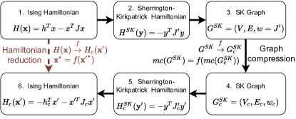
Figure 1: Hamiltonian reduction via compressing non-separable groups in SK graph.

III Non-separability Theory and
Graph-based Hamiltonian Reduction

In this section, we propose a Hamiltonian reduction framework via graph compression as shown in Fig. 1. First, we convert Ising Hamiltonian into Sherrington-Kirkpatrick (SK) Hamiltonian, and then SK graph that minimum-cut induces the ground state for the Hamiltonian. We then develop non-separability theory for SK graph and show how compressing non-separable groups in the graph can lead to efficient Hamiltonian reduction.

III-A Minimum-cut on Sherrington-Kirkpatrick (SK) Graphs

We introduce a new graph, called Sherrington-Kirkpatrick (SK) graph that encloses both the coupling strengths and the external fields in an Ising Hamiltonian. More importantly, finding the weighted mininmum-cut on the SK graph is equivalent to finding the ground state of the Ising Hamiltonian. Thus, the SK graph provides a pure graph theory tool for minimizing the energy of Ising Hamiltonians.

Construction

Given an Ising Hamiltonian $H(\mathbf{x})=\mathbf{h}^{T}\mathbf{x}+\mathbf{x}^{T}\mathbf{J}\mathbf{x}$ with $n$ variables, the SK graph of $H(\mathbf{x})$ is denoted by $G^{SK}_{H}=(V,E,w)$. The set of nodes $V=\{1,2,\ldots,n,n+1\}$ in which nodes $1,2,\ldots,n$ correspond to the variables $x_{1},x_{2},\ldots,x_{n}$ in the Hamiltonian. Node $(n+1)$ is added to capture the external fields $\mathbf{h}$. The set of undirected edges $E$ consists of undirected edges $(i,j)$ with weight $w_{ij}=J_{ij}+J_{ji}$ for $1\leq i,j\leq n$ and $(i,n+1)$ with weights $w_{i,n+1}=h_{i}$. For efficiency, we only retain in $E$ edges with non-zero weights.

We denote by $\mathbf{J^{\prime}}$ the weighted adjacency matrix of $G^{SK}$. $\mathbf{J^{\prime}}$ can be seen as the result of appending the external fields $\mathbf{h}$ to the right of $\mathbf{J}$ (after assigning $J_{ij}=J_{ij}+J_{ji},J_{ji}=0$ for $i<j$). For $\mathbf{y}\in\mathbb{S}^{n+1}$, $\mathbf{J^{\prime}}$ corresponds to a Hamiltonian

$$H^{SK}(\mathbf{y})=-\mathbf{y}^{T}\mathbf{J^{\prime}}\mathbf{y}.$$

$H^{SK}$ contains no external fields and is in a form of a Sherrington-Kirkpatrick Hamiltonian [31], hence, we named the constructed graph SK graph. In fact, we can prove that

$$\min_{\mathbf{y}\in\mathbb{S}^{n+1}}H^{SK}(\mathbf{y}) =\min_{\mathbf{y}\in\mathbb{S}^{n+1}}-\mathbf{y}^{T}\mathbf{J^{\prime}}\mathbf{y}$$

$$=\min_{\mathbf{y}\in\mathbb{S}^{n+1}}-\sum_{1\leq i,j\leq n}J_{ij}y_{i}y_{j}-y_{n+1}\sum_{1\leq i\leq n}h_{i}y_{i}$$

$$=\min_{\mathbf{x}\in\mathbb{S}^{n}}H(\mathbf{x}).$$ (4)

The last equality holds as we can always replace $\mathbf{y}$ with $-\mathbf{y}$ to ensure $y_{n+1}=1$ without changing the energy of the Hamiltonian $H^{SK}(\mathbf{y})$.

Equivalence between minimizing energy and weighted min-cut (WMC) on SK graph

For any subset $S\subseteq V$, $S$ induces a cut $\langle S,V\setminus S\rangle$, consisting of the edges crossing $S$ and $V\setminus S$. The capacity of the cut is defined as

$$c(S)=\sum_{(u,v)\in\langle S,V\setminus S\rangle}w_{uv}.$$

We consider the following variation of the weighted min-cut (WMC) problem of finding

$$mc(G)=\arg\min_{S\subseteq V}c(S).$$

Remark that the cut space includes the empty cut $S=\emptyset$ (or equivalently $S=V$). This is different from the standard minimum-cut problem in which cuts often contain at least one node on each side. For example, since $c(\emptyset)=0$, it follows that,

$$MC(G)=\min_{S\subseteq V}c(S)\leq 0,$$

where $MC(G)$ denotes the minimum capacity of any cut. Thus, min-cuts in WMC often have negative capacities.

There is a one-to-one mapping between the capacity of the cut in $G^{SK}$ to the energy of the Hamiltonian $H^{SK}$. Define for a subset $S\subseteq V$, the corresponding vector $\mathbf{y}^{(S)}\in\mathbb{S}^{n+1}$, in which for $v\in V$

$$y_{v}^{(S)}=\begin{cases}+1&\text{ if }v\in S,\\ -1&\text{ if }v\notin S,.\end{cases}$$

We have,

$$c(S) =\sum_{(u,v)\in\langle S,V\setminus S\rangle}w_{uv}=\frac{1}{4}\sum_{(u,v)\in E}w_{uv}(y_{u}^{(S)}-y_{v}^{(S)})^{2}$$

$$=-\frac{1}{2}\sum_{(u,v)\in E}w_{uv}s_{u}s_{v}+\frac{1}{2}\sum_{(u,v)\in E}w_{uv}$$

$$=H^{SK}(\mathbf{y}^{(S)})+c_{w},$$

where $c_{w}=\frac{1}{2}\sum_{\left(u,v\right)\in E}w_{uv}=\frac{1}{2}\sum_{i,j}J^{\prime}_{ij}$ is a fixed value that depends only on $w$.

Thus, finding the lowest energy of Hamiltonian $H^{SK}$ and $H(\mathbf{x})$ (from Eq. 4) is the same as finding the WMC on $G^{SK}$.

Lemma III.1.

For $c_{w}=\frac{1}{2}\sum_{i,j}J^{\prime}_{ij}$,

$$\min_{\mathbf{x}\in\mathbb{S}^{n}}H(\mathbf{x})=\min_{\mathbf{y}\in\mathbb{S}^{n+1}}H^{SK}(\mathbf{y})=MC(G)-c_{w}.$$

Deriving minimum energy configuration from min-cut

Let $S^{*}=mc(G^{SK})$ and $\mathbf{x}^{(S^{*})}$ be the vector obtained from $\mathbf{y}^{(S^{*})}$ by removing the $(n+1)$th element $y^{(S^{*})}_{n+1}$. If $y^{(S^{*})}_{n+1}=-1$, we multiply $\mathbf{x}^{(S^{*})}$ with $-1$. We can verify that

$$H(\mathbf{x}^{(S^{*})})=\min_{\mathbf{x}\in\mathbb{S}^{n}}H(\mathbf{x})$$ (5)

SK graph vs. Hamiltonian/QUBO graphs

The Hamiltonian graph induced by $\mathbf{J}$ does not contain the information on the external fields and, thus, can not represent the Hamiltonian, standing alone. The QUBO obtained by converting the Hamiltonian to a QUBO formulation has edge weights that are different from the coupling strengths in the hardware. Hence, it may not reflect the physical interactions among the sites. In contrast, the SK graph encloses both the external fields and coupling strengths (that are close to the implemented ones on the hardware). It enables the exploration of the Hamiltonian’s energy landscape via exploring the cut space on the SK graph.

III-B Non-separable Groups (NGs)

We introduce new notions of non-separable groups (NGs) in a weighted undirected graph, non-separability index, and a Hamiltonian reduction framework based on identifying non-separable groups.

Let $G=(V,E,w)$ be a weighted undirected graph, e.g, the SK graph of some Ising Hamiltonian. A subset $X\subseteq V$ is called a non-separable group, if all min-cuts on $G$ will have all nodes in $X$ on one side. Here, we use min-cut to refer to an optimal cut for the WMC problem on $G$. If $X$ stays completely on one side of some (but not all) min-cuts, we say $X$ is a weakly non-separable group. As we will show in the next subsection, all nodes in a (weakly) non-separable group can be merged into a single node, creating a smaller graph. Importantly, any min-cut in the smaller graph can be easily extended to a min-cut in $G$.

Properties of non-separable groups

We show the basic properties of non-separable groups, including hereditary, and the closesure under intersection and union.

Lemma III.2.

Let $X,Y$ be non-separable groups on $G$.

1. Hereditary. Any subset of $S\subseteq X$ is also non-separable. This statement also holds when $X$ is a weakly non-separable group.

2. Closure under intersection and union. Both $X\cap Y$ and $X\cup Y$ are non-separable. The statement also holds when only one of $X$ or $Y$ is non-separable and the other is weakly non-separable.

The proof comes directly from the definition of non-separable and weakly non-separable groups.

Non-separability index

We propose a measure, termed non-separability index, to quantify how “difficult” to separate a group of nodes $X\subseteq V$. Here, we say a cut $S\subseteq V$ separates a set $X$ if there exist two nodes $u,v\in X$ such that $u\in S$ and $v\notin S$. Formally,

Definition III.3 (Separation).

Consider a cut $S\subseteq V$ and a subset $X\subseteq V$, we say $S$ separates $X$, denoted by, $S\ominus X$ iff

$$X\cap S\notin\{\emptyset,X\}.$$

We also denote by $sep(X)=\{S\subseteq V:S\ominus X\}$ the collection of all cuts in $G$ that separate $X$.

The non-separability index of $X$ is defined as the difference between the minimum capacities of the cuts in $sep(X)$ and those outside $sep(X)$.

Definition III.4 (Non-separability index).

Given a graph $G$ and a subset $X\subseteq V$, the non-separability index of $X$ is defined as

$$\nu_{G}(X)=\min_{S^{\prime}\in sep(X)}c(S^{\prime})-\min_{S\subset V,S\notin sep(X)}c(S).$$ (6)

For a non-separable group $X$, the non-separability index is the minimum increase in the cut capacity to turn some min-cut into a new cut that separates $X$. If $G$ is a SK graph for some Hamiltonian $H(\mathbf{x})$, the non-separability index of $X$ corresponds to the energy gap between the ground state and the next excited state that separates $X$, i.e., having two spins in $X$ with opposite signs.

The non-separability index $\nu_{G}(X)$ acts as an indicator on whether node groups are non-separable. When the context is clear, we omit the graph $G$ and write $\nu(X)$.

Theorem III.5 (Non-separability conditions).

Given a group of nodes $X\subseteq V$,

• $X$ is a non-separable group iff $\nu(X)>0$.

• $X$ is a weakly non-separable group iff $\nu(X)=0$.

Proof.

We prove the first statement. If $X$ is a non-separable group, it follows that none of the min-cuts can appear in $sep(X)$. From Eq. 6, we have

$$\nu(X) =\min_{S^{\prime}\in sep(X)}c(S^{\prime})-\min_{S\subset V,S\notin sep(X)}c(S)$$

$$=\min_{S^{\prime}\in sep(X)}c(S^{\prime})-\min_{S\subseteq V}c(S)>0.$$

Vice versa, if $\nu(X)>0$, none of the min-cuts can appear in $sep(X)$ (otherwise $\nu(X)\leq 0$).

Similarly, we can show the second statement by noting that $\nu(X)=0$ iff min-cuts appear both in $sep(X)$ and out of $sep(X)$. ∎

Antipolar pair

Consider a special case when $X$ contains a pair of nodes $u$ and $v$. There are three possible cases for the value of $\nu(X)$: 1) $\nu(X)>0$, $X$ is a non-separable group; 2) $\nu(X)=0$, $X$ is a weakly non-separable group; and 3) $\nu(X)<0$, in this case, we say $u$ and $v$ is an antipolar pair. For an antipolar pair $u,v$, we have, by Eq. 6, all min-cuts must belong to $sep(X)$ (otherwise $\nu(X)\geq 0$). In other words, an antipolar pair always stay in different sides in all min-cuts.

As we will show in next subsection, by negating the weights of all edges incident at $u$ (or $v$), we can turn $u$ and $v$ into a non-separable pair in the new graph.

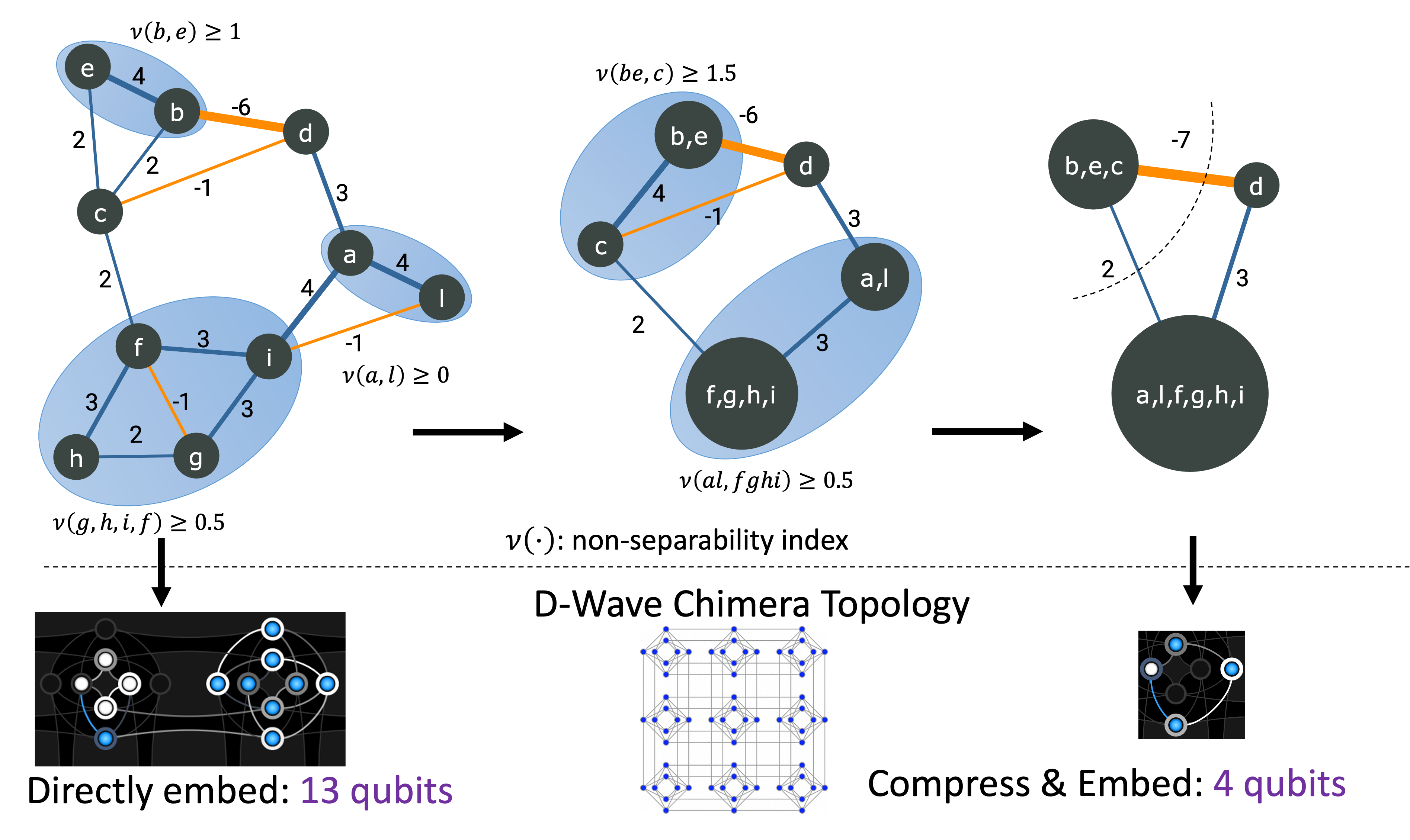
Figure 2: An example of graph compression framework via non-separability theory. The compression reduce the physical qubits by 3+ folds (a 69% reduction ratio).

III-C Hamiltonian Reduction by Compressing NGs

As shown in Fig. 1, after converting an Ising Hamiltonian into a SK graph $G^{SK}=(V,E,w)$, we will compress non-separable groups (NGs) in $G^{SK}$ into a smaller graph $G^{SK}_{c}$ that helps us construct the Hamiltonian reduction.

At a high glance, our graph compression framework consists of three steps. First, we identify NGs and antipolar pairs, for example, using methods presented in Section IV. Second, we apply the non-separability theory, especially the hereditary and the closure under the union, to enlarge NGs. Finally, we merge each NG into a single node then apply a flip operation to turn antipolar pairs into non-separable pairs that are further merged into single nodes. The three steps are repeated until no further NGs or antipolar pairs are detected as shown in Fig. 2.

III-C1 Identification of NGs and antipolar pairs

In this step, we search on $G^{SK}$ to identify NGs, weakly NGs, and antipolar pairs, for example, using the algorithm in Section IV. We denote by $\mathcal{X}_{s}$, $\mathcal{X}_{w},$ and $\mathcal{R}$ the sets of found NGs, weakly NGs, and antipolar pairs, respectively.

III-C2 Enlarging NGs and antipolar pairs

By applying the closure of NGs and weakly NGs under union, we can enlarge and combine the identified NGs, weakly NGs. Specifically, we apply the following rules:

• if $X$ and $Y$ are two NGs, $X\cup Y$ is an NG (Lemma III.2).

• if $x$ and $y$ is an antipolar pair and $y\in Y$ for some NG $Y$, then for all $z\in Y$, $x,z$ is an antipolar pair.

• if $x,y$ and $y,z$ are two antipolar pairs, $\{x,z\}$ is an NG.

We can use a linear-time algorithm, similar to a node coloring algorithm in a bipartite graph, to repeat the above rules until no further extension is possible. In addition, the above rules can also be extended to include weakly NGs.

III-C3 Compression of NGs and antipolar pairs

We present compression of NGs, weakly NGs, and antipolar pairs. In a single round, we will ignore weakly NGs unless there are no NGs nor antipolar pairs. To preserve min-cuts, we can only compress one weakly NG at a time and have to repeat the identification steps. In contrast, multiple NGs and antipolar pairs can be compressed simultaneously in a single round.

Compression of an NG (or weakly NG) to a single node

The compression of an NG (or weakly NG) $X$ is done simply by merging nodes in $X$ into a single nodes. Parallel edges will be resolved by aggregating the weights.

Compression of an antipolar pair

An antipolar pair $u,v$ is compressed by first, flipping node $u$ (or $v$), followed by merging of $u$ and $v$. The flip of node $u$ is done by negating the weights of all edges incident at $u$.

Due to the space limit, we omit the proofs on the correctness of the enlarging and compression steps. However, most of the proofs are due to the fact that compression of NGs will preserve min-cuts as each NG will never be separated by any min-cut in the first place.

IV Fast Hamiltonian Reduction (FastHare)

We propose FastHare algorithm, an instance of the compression framework in Section III with the focus on fast running time. FastHare limits the search to small-size NGs. Further, it uses a nested collection of fast and tight-but-expensive bounds in scanning for potential NGs.

It follows by efficient bounds for small-size NGs of size $2$ and $3$ in Subsection IV-B. Third, we present in Subsection IV-C, the efficient search techniques in FastHare that limit the time complexity to $O(\alpha n^{2})$ IV-B. Finally, Subsection IV-D provides the complexity analysis.

IV-A Bounds to Prove Non-separability

We begin with a lower bound for the non-separability index for groups of any size. The bound will be used in FastHare to determine whether a group is an NG.

We define some necessary notations. Given an undirected and weighted graph $G=(V,E,w)$, we extend $w_{uv}$ to define $w_{uv}=0$ if $(u,v)\notin E$. For a node $u\in V$, we denote by ${\mathbf{w}}^{(u)}=({\mathsf{w}}_{u1},\cdots,{\mathsf{w}}_{un})$ the weight vector of the node $u$ and by $\|{\mathbf{w}}^{(u)}\|=\sum_{v=1}^{n}|{\mathsf{w}}_{uv}|$ the 1-norm of ${\mathbf{w}}^{(u)}$. We also define ${\mathsf{c}_{|.|}}(S,T)=\sum_{u\in S,v\in T}|{\mathsf{w}}_{uv}|$, the total absolute values of weights over all edges between $S$ and $T$.

Lemma IV.1 (Non-separability index lower bound).

Consider a graph $G=(V,E,w)$ and a set $X\subseteq V$, we have

$$\nu_{G}(X)\geq\hat{\nu}_{G}(X)=\min_{Z\subset X,Z\neq\emptyset}({\mathsf{c}}(Z,X\setminus Z)-P_{X}(Z)),$$

where

$$P_{X}(Z)=\min\big{(}\frac{1}{2}\sum_{u\in Y}\left|\sum_{v\in Z}{\mathsf{w}}_{uv}-\sum_{v\in X\setminus Z}{\mathsf{w}}_{uv}\right|,$$

$${\mathsf{c}_{|.|}}(Z,Y),{\mathsf{c}_{|.|}}(X\setminus Z,Y)\big{)},$$

and $Y=\bar{X}=V\setminus X$.

Proof.

Based on Def. III.4, we have,

$$\nu_{G}(X)\geq\min_{S\subseteq V,S\ominus X}\left(C\left(S\right)-\min\left(C\left(S\setminus X\right),C\left(\bar{S}\setminus X\right)\right)\right)$$

For any set $S\subseteq V,s.t.,S\ominus X$, let $T=\bar{S}=V\setminus S$. Let $X_{S}=X\cap S,X_{T}=X\cap T$ be the intersections of $X$ and $S,T$, respectively. Let $Y_{S}=S\setminus X_{S},Y_{T}=T\setminus X_{T}$ be the intersections of $Y$ and $S,T$, respectively.

We have

$${\mathsf{c}}(S)-\min({\mathsf{c}}(S\setminus X),{\mathsf{c}}(T\setminus X))$$

$$=\max({\mathsf{c}}(S)-{\mathsf{c}}(S\setminus X),{\mathsf{c}}(S)-{\mathsf{c}}(T\setminus X))$$

$$=\max({\mathsf{c}}(X_{S},X_{T})+{\mathsf{c}}(X_{S},Y_{T})-{\mathsf{c}}(X_{S},Y_{S}),$$

$$\quad\quad\quad\quad{\mathsf{c}}(X_{T},X_{S})+{\mathsf{c}}(X_{T},Y_{S})-{\mathsf{c}}(X_{T},Y_{T}))$$

$$={\mathsf{c}}(X_{S},X_{T})-\min({\mathsf{c}}(X_{S},Y_{S})-{\mathsf{c}}(X_{S},Y_{T}),$$

$$\quad\quad\quad\quad\quad\quad\quad\quad\quad\quad{\mathsf{c}}(X_{T},Y_{T})-{\mathsf{c}}(X_{T},Y_{S}))$$

Let $Q(S)=\min({\mathsf{c}}(X_{S},Y_{S})-{\mathsf{c}}(X_{S},Y_{T}),{\mathsf{c}}(X_{T},Y_{T})-{\mathsf{c}}(X_{T},Y_{S})).$ We have,

$$Q(S) \leq\frac{1}{2}({\mathsf{c}}(X_{S},Y_{S})-{\mathsf{c}}(X_{S},Y_{T})$$

$$\quad\quad+{\mathsf{c}}(X_{T},Y_{T})-{\mathsf{c}}(X_{T},Y_{S}))$$

$$=\frac{1}{2}\sum_{u\in Y_{S}}\left(\sum_{v\in X_{S}}{\mathsf{w}}_{uv}-\sum_{v\in X_{T}}{\mathsf{w}}_{uv}\right)$$

$$\quad\quad+\frac{1}{2}\sum_{u\in Y_{T}}\left(\sum_{v\in X_{T}}{\mathsf{w}}_{uv}-\sum_{v\in X_{S}}{\mathsf{w}}_{uv}\right)$$

$$\leq\frac{1}{2}\sum_{u\in Y_{S}}\left|\sum_{v\in X_{S}}{\mathsf{w}}_{uv}-\sum_{v\in X_{T}}{\mathsf{w}}_{uv}\right|$$

$$\quad\quad+\frac{1}{2}\sum_{u\in Y_{T}}\left|\sum_{v\in X_{S}}{\mathsf{w}}_{uv}-\sum_{v\in X_{T}}{\mathsf{w}}_{uv}\right|$$

$$\leq\frac{1}{2}\sum_{u\in Y}\left|\sum_{v\in X_{S}}{\mathsf{w}}_{uv}-\sum_{v\in X_{T}}{\mathsf{w}}_{uv}\right|$$

Further, we have,

$$Q(S) \leq\min({\mathsf{c}_{|.|}}(X_{S},Y_{S})+{\mathsf{c}_{|.|}}_{(}X_{S},Y_{T}),$$

$$\quad\quad\quad\quad{\mathsf{c}_{|.|}}(X_{T},Y_{T})+{\mathsf{c}_{|.|}}(X_{T},Y_{S}))$$

$$=\min({\mathsf{c}_{|.|}}(X_{S},V\setminus X),{\mathsf{c}_{|.|}}(X_{T},V\setminus X))$$

Therefore, we have, $Q(S)\leq P_{X}(X_{S}).$

Thus, we have,

$${\mathsf{c}}(S)-\min({\mathsf{c}}(S\setminus X),{\mathsf{c}}(T\setminus X)) ={\mathsf{c}}(X_{S},X_{T})-Q(S)$$

$$\geq{\mathsf{c}}(X_{S},X_{T})-P_{X}(X_{S}).$$

Hence, we have,

$$\nu_{G}(X) \geq\min_{S\subseteq V,S\ominus X}\left(C\left(S\right)-\min\left(C\left(S\setminus X\right),C\left(T\setminus X\right)\right)\right)$$

$$\geq\min_{S\subseteq V,S\ominus X}({\mathsf{c}}(X_{S},X_{T})-P_{X}(X_{S}))$$

$$=\min_{Z\subset X,Z\neq\emptyset}({\mathsf{c}}(Z,X\setminus Z)-P_{X}(Z)).$$

∎

IV-B Efficient search for NGs

Now, we use the non-separability index lower bound in Lemma IV.1 to search for non-separable and antipolar pairs of sizes $2$ and $3$.

Non-separable pair identification. Consider an edges $(u,v)\in E$. Our goal is to determine the relation between $u$ and $v$, whether they make an NG, a weakly NG, or an antipolar pair. For an edge $(u,v)\in E$, we define fast score ${\mathsf{\hat{\nu}_{f}}}$ and similarity score ${\mathsf{\hat{\nu}_{s}}}$ for $(u,v)$ as follows

$${\mathsf{\hat{\nu}_{f}}}(u,v)=2|{\mathsf{w}}_{uv}|-\min(\|{\mathbf{w}}^{(u)}\|,\|{\mathbf{w}}^{(v)}\|),$$ (7)

$${\mathsf{\hat{\nu}_{s}}}(u,v)=\begin{cases}2|{\mathsf{w}}_{uv}|-\frac{1}{2}\|{\mathbf{w}}^{(u)}-{\mathbf{w}}^{(v)}\|&\text{ if }{\mathsf{w}}_{uv}\geq 0,\\ 2|{\mathsf{w}}_{uv}|-\frac{1}{2}\|{\mathbf{w}}^{(u)}+{\mathbf{w}}^{(v)}\|&\text{ if }{\mathsf{w}}_{uv}<0.\\ \end{cases}$$ (8)

Lemma IV.2.

Consider a graph $G=(V,E,w)$. For any edges $(u,v)\in E$, we have:

• If $\max({\mathsf{\hat{\nu}_{f}}}(u,v),{\mathsf{\hat{\nu}_{s}}}(u,v))>0$,

  • if ${\mathsf{w}}_{uv}\geq 0$, $\{u,v\}$ is an NG,

  • if ${\mathsf{w}}_{uv}<0$, $(u,v)$ is an antipolar pair.

• If $\max({\mathsf{\hat{\nu}_{f}}}(u,v),{\mathsf{\hat{\nu}_{s}}}(u,v))=0$ and ${\mathsf{w}}_{uv}\geq 0$, $\{u,v\}$ is classified as a weakly NG.

Proof.

Let $X=\{u,v\}$ and $Y=V\setminus X$. We consider two cases of ${\mathsf{w}}_{uv}$ as follows.

Case 1: ${\mathsf{w}}_{uv}\geq 0$. Based on Lemma IV.1, we have,

$$\nu_{G}(X) \geq{\mathsf{w}}_{uv}-\min(\frac{1}{2}\sum_{z\in Y}|{\mathsf{w}}_{uz}-{\mathsf{w}}_{vz}|,$$

$$\quad\quad\quad\quad\quad\quad{\mathsf{c}_{|.|}}(\{u\},Y),{\mathsf{c}_{|.|}}(\{v\},Y))$$

$$=2{\mathsf{w}}_{uv}-\min(\frac{1}{2}\|{\mathbf{w}}^{(u)}-{\mathbf{w}}^{(v)}\|,\|{\mathbf{w}}^{(u)}\|,\|{\mathbf{w}}^{(v)}\|)$$

$$=\max({\mathsf{\hat{\nu}_{f}}}(u,v),{\mathsf{\hat{\nu}_{s}}}(u,v))$$

Thus, we have:

• If $\max({\mathsf{\hat{\nu}_{f}}}(u,v),{\mathsf{\hat{\nu}_{s}}}(u,v))>0$, $\{u,v\}$ is an NG.

• If $\max({\mathsf{\hat{\nu}_{f}}}(u,v),{\mathsf{\hat{\nu}_{s}}}(u,v))=0$, $\{u,v\}$ is classified as a weakly NG.

Case 2: ${\mathsf{w}}_{uv}<0$. Let $G^{\prime}={\mathsf{flip}}(G,v)$. Similar to Case 1, we have,

$$\nu_{G^{\prime}}(X)\geq\max({\mathsf{\hat{\nu}_{f}}}(u,v),{\mathsf{\hat{\nu}_{s}}}(u,v)).$$

Thus, if $\max({\mathsf{\hat{\nu}_{f}}}(u,v),{\mathsf{\hat{\nu}_{s}}}(u,v))>0$, $\{u,v\}$ is an NG in $G^{\prime}$. In other words, $(u,v)$ is an antipolar pair in $G$. ∎

Non-separable triple identification. Consider a group of three nodes $X=\{u,v,z\}$ that has at least 2 edges among the nodes. Apply the lower bound on the non-separability index $\hat{\nu}_{G}(X)$ in Lemma IV.1 on $X$, we have

$$\hat{\nu}_{G}(X)<\min_{Z\subset X,Z\neq\emptyset}({\mathsf{c}}(Z,X\setminus Z))\leq MC(G[X]),$$

where $G[X]$ is the subgraph induced by $X$ in $G$.

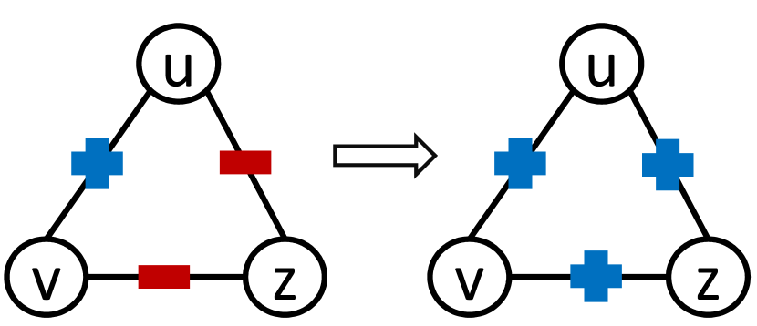
(a) The number of edges with negative weight is even. All edges have non-negative weights after flipping.

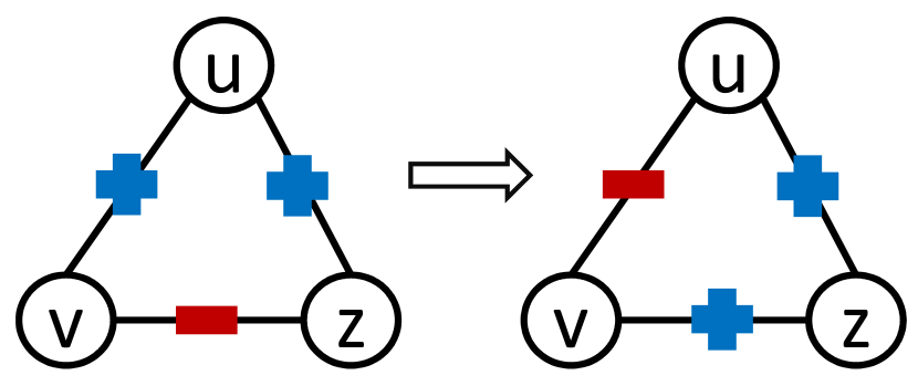
(b) The number of negative weights is odd. The edge $(u,v)$ (with the smallest absolute weight) has a negative weight after flipping.

Figure 3: Flipping nodes in $X=\{u,v,z\}$ to ensure the WMC on the induced graph on $X$ is non-negative.

Recall that, we can only find the relation among the nodes in $X$ if the $\hat{\nu}_{G}(X)\geq 0$. Hence, we will flip the nodes in $X$ such that the WMC in the subgraph induced by $X$ is non-negative. As every time we flip a node in $X$, we always change the signs of two edges in $G[X]$, the parity on the number of negative weight edges remain the same. Thus, we consider two cases based on the number of edges with negative weight (see Fig. 3).

• Case 1: The number of edges with negative weight is even. In this case, we can flip the nodes in $X$ such that all edges in $G[X]$ is non-negative. Thus, the WMC of $G[X]$ is non-negative.

• Case 2: The number of edges with negative weight is even. In this case, we can flip the nodes in $X$ such that only the edge, with the smallest absolute weight, has a negative weight after flipping. Now, the WMC of $G[X]$ is also non-negative.

Let $\bar{X}\subseteq X$ be the set of nodes that we need to flip so that the WMC of $G[X]$ is also non-negative. Let $G^{\prime}={\mathsf{flip}}_{\tilde{X}}(G)$ and $\tilde{{\mathsf{w}}}_{uv},\tilde{{\mathsf{w}}}_{uz},\tilde{{\mathsf{w}}}_{vz}$ be the weight of $(u,v)$, $(u,z)$, $(v,z)$, respectively, on $G^{\prime}$. We define the triangle score ${\mathsf{\hat{\nu}_{t}}}$ as follows.

$${\mathsf{\hat{\nu}_{t}}}(X) =\min_{x\in X}\big{(}\sum_{y\in X\setminus\{x\}}\tilde{{\mathsf{w}}}_{xy}-\min\big{(}\|{\mathbf{w}}^{(x)}\|-\sum_{y\in X\setminus\{x\}}|{\mathsf{w}}_{xy}|,$$

$$\quad\quad\quad\sum_{y\in X\setminus\{x\}}\big{(}\|{\mathbf{w}}^{(y)}\|-\sum_{z\in X\setminus\{y\}}|{\mathsf{w}}_{yz}|\big{)}\big{)}\big{)}$$ (9)

Lemma IV.3.

Consider a graph $G=(V,E,w)$ and any set $X\subseteq V$ of size $3$. Let $\bar{X}\subseteq X$ be the set of nodes that we need to flip so that the WMC of $G[X]$ is also non-negative. If ${\mathsf{\hat{\nu}_{t}}}(X)>0$, we have:

• $\tilde{X}$ and $X\setminus\tilde{X}$ are NG groups.

• $\forall u\in\tilde{X},v\in X\setminus\tilde{X}$, $(u,v)$ is an antipolar pair.

Proof.

Let $G^{\prime}={\mathsf{flip}}_{\tilde{X}}(G)$ and $\tilde{{\mathsf{w}}}_{uv},\tilde{{\mathsf{w}}}_{uz},\tilde{{\mathsf{w}}}_{vz}$ be the weight of $(u,v)$, $(u,z)$, $(v,z)$, respectively, on $G^{\prime}$. Let $Y=V\setminus X$, we have,

$$\hat{\nu}_{G^{\prime}}(X) \geq\min_{x\in X}\big{(}\sum_{y\in X\setminus\{x\}}\tilde{{\mathsf{w}}}_{xy}-\min({\mathsf{c}_{|.|}}(\{x\},Y),$$

$$\quad\quad\quad\quad\quad{\mathsf{c}_{|.|}}(X\setminus\{x\},Y))\big{)}$$

$$=\min_{x\in X}\big{(}\sum_{y\in X\setminus\{x\}}\tilde{{\mathsf{w}}}_{xy}-\min\big{(}\|{\mathbf{w}}^{(x)}\|-\sum_{y\in X\setminus\{x\}}|{\mathsf{w}}_{xy}|,$$

$$\quad\quad\quad\sum_{y\in X\setminus\{x\}}\big{(}\|{\mathbf{w}}^{(y)}\|-\sum_{z\in X\setminus\{y\}}|{\mathsf{w}}_{yz}|\big{)}\big{)}\big{)}$$

$$={\mathsf{\hat{\nu}_{t}}}(X).$$

If ${\mathsf{\hat{\nu}_{t}}}(X)>0$, $X$ is an NG on $G^{\prime}$. Thus, $\tilde{X}$ and $X\setminus\tilde{X}$ are NGs. And $\forall u\in\tilde{X},v\in X\setminus\tilde{X}$, $(u,v)$ is an antipolar pair. ∎

IV-C FastHare algorithm

We now describe the FastHare algorithm to reduce the Hamiltonian. The algorithm follows the compression framework (see Fig 1) in Section III. It transforms the Hamiltonian reduction task into a graph compression problem. Its main algorithm also consists of multiple rounds, each round consists of three steps: 1) identification of NGs, weakly NGs, and antipolar pairs 2) enlarging step, and 3) compression step.

The identification of NGs is done by computing fast scores, the similarity scores, and the triangle scores for groups of 2 and 3 nodes in the graph. The main trick is to levarage fast score, that can be computed and maintained efficiently after merging and flipping, to guide the search for potential edges and triangles and attemp to prove their non-separability with more expensive bounds/scores. The pseudocode of the FastHare algorithm is given in Algorithm 1.

Input : A graph $G=(V,E,w)$ and a parameter $\alpha$

Output : A compressed graph.

1 Compute the fast score ${\mathsf{\hat{\nu}_{f}}}(u,v)\forall(u,v)\in E$  Add top $n\alpha$ edges with the highest fast score to a list $L$

2 Compute the similarity score for all edges in $L$

3 For $(u,v)\in L$ and $w\in{\mathsf{adj}}(u)\cup{\mathsf{adj}}(v)$, compute ${\mathsf{\hat{\nu}_{t}}}(\{u,v,z\}$

4 repeat

5       Obtain $\mathcal{X}_{s},\mathcal{X}_{w},\mathcal{R}$ from pairs and triples with non-negative updated scores (Lemmas IV.2 and IV.3)

6      

7      Compress the graph $G$ based on the list $\mathcal{X}_{s},\mathcal{X}_{w},\mathcal{R}$ using the compression in Subsection III-C3

8       Update the scores and the list $L$ on the new graph

9      

10until  $\mathcal{X}_{s},\mathcal{X}_{w},\mathcal{R}=\emptyset$ ;

Return $G$

Algorithm 1 Algorithm FastHare.

Initialization (Lines 1-3, Alg. 1)

The FastHare algorithm starts with an initialization phase, followed by a loop of iterations to reduce the Hamiltonian. In the initialization phase, we compute the fast score (Eq. 7) for all edges and select the top $n\alpha$ edges with the highest fast score to a list $L$. Then, we compute the similarity score for all edges in $L$ and the triangle score for the groups that have at least one edges in $L$.

Iterative compression (Lines 5-7, Alg. 1)

In each iteration, we obtain the collection of NGs $\mathcal{X}_{s}$, the collection of weakly NGs $\mathcal{X}_{w}$, and the collection of antipolar pairs $\mathcal{R}$ from pairs and triples with non-negative updated scores (Lemmas IV.2 and IV.3). The scores are computed in the previous iteration (or the initialization for the first iteration). Then, we compress the graph $G$ based on the list $\mathcal{X}_{s},\mathcal{X}_{w},\mathcal{R}$ using the compression in Subsection III-C3. Finally, we update the scores and the list $L$ on the new graph.

Efficiently maintaining the score. For each node $v\in V$, we maintain a value $A_{v}=\|{\mathbf{w}}^{(v)}\|.$ Plus, for each edge $(u,v)\in L$, we maintain a value $B_{uv}=B^{\prime}_{uv}-|{\mathsf{w}}_{uz}|-|{\mathsf{w}}_{vz}|$, where

$$B^{\prime}_{uv}=\begin{cases}\sum_{z\in{\mathsf{adj}}_{u}\cap{\mathsf{adj}}_{v}}|{\mathsf{w}}_{uz}-{\mathsf{w}}_{vz}|&\text{ if }{\mathsf{w}}_{uv}\geq 0,\\ \sum_{z\in{\mathsf{adj}}_{u}\cap{\mathsf{adj}}_{v}}|{\mathsf{w}}_{uz}+{\mathsf{w}}_{vz}|&\text{ if }{\mathsf{w}}_{uv}<0,\end{cases}$$

where ${\mathsf{adj}}_{v}$ is the set of neighbors of the node $v$.

For any pair $(u,v)\in E$, we can compute the fast score

$${\mathsf{\hat{\nu}_{f}}}(u,v)=2|{\mathsf{w}}_{uv}|-\min(A_{u},A_{v}).$$

For any pair $(u,v)\in L$, we can compute the similarity score

$${\mathsf{\hat{\nu}_{s}}}(u,v)=2|{\mathsf{w}}_{uv}|-\frac{1}{2}(A_{u}+A_{v}+B_{uv}).$$

The triangle score of a group $X$ can also be computed based on the values of $A$.

Updating the scores after flipping a node. After flipping a node $u$, $\forall v\in V$ the value $A_{v}$ does not change. We only need to update the value of $B_{uv}$ for all $(u,v)\in L$ such that $v\in{\mathsf{adj}}_{u}$. For the edge $(v,z)\in L$ such that $v,z\in{\mathsf{adj}}_{u}$, the value of $B_{uv}$ does not changed since the sign of both ${\mathsf{w}}_{uv}$ and ${\mathsf{w}}_{uz}$ are changed.

Updating the scores after merging two nodes. After merging two nodes $(x,y)$ to a new node $z$. We compute the new value of $A_{z}$ and update the value $A_{u}$ for all $u\in{\mathsf{adj}}_{x}\cup{\mathsf{adj}}_{y}$. For the similarity score, we remove all edges in $L$ that one endpoint is $x$ or $y$. Then we update $B_{uv}$ for all edges $(u,v)\in L$ such that both $u$ and $v$ are adjacent to $x$ or $y$. We also add at most $\alpha$ edges from $z$ with the highest fast score to $L$ and update the value $B$ of those edges. This limitation on the number of updated edges is important to keep the running time bounded by $O(\alpha n^{2}$).

IV-D Complexity analysis

Lemma IV.4.

The time complexity of the FastHare algorithm (Algorithm 1) is $O(n^{2}\alpha)$

Proof.

For the initialization, the time complexity to compute the fast score, the similarity score, and the triangle score is $O(n^{2})$, $O(n^{2}\alpha)$, and $O(n^{2}\alpha)$, respectively.

For the iterative compression, after flipping a node $u$, we only need to compute for all $(u,v)\in L$ such that $v\in{\mathsf{adj}}_{u}$. Thus, the cost to update the scores after a flipping is $O(n\alpha)$. After the merging two nodes $(x,y)$ to a node $z$, we update the score for all edges $(u,v)\in L$ such that both $u$ and $v$ are adjacent to $x$ or $y$ and the top $\alpha$ edges from $z$ with the highest fast score. Thus, the cost to update after a merging is $O(n\alpha)$. In FastHare the total number of flipping/merging is $n$. Thus, the total time complexity to update the score is $O(n^{2}\alpha)$. Plus, in each iteration, we only check for the pairs and triplets that have the scores updated. Thus, the time complexity to check the pairs and triplets is $O(n^{2}\alpha)$.

Therefore, in total, the time complexity of the FastHare algorithm is $O(n^{2}\alpha)$. ∎

V Experiment

We perform numerical experiments to assess the performance of the proposed methods in terms of reduction ratio and processing time. Further, we analyze characteristics of the benchmarked instances to identify factors that are important for the reducibility of Hamiltonian.

V-A Experiments settings

Algorithms. We compare FastHare algorithm, that is described in Section IV with the implementation of D-Wave’s SDK. The implementation of D-Wave’s SDK applies a roof duality technique [20] to minimizing assignments for some of the variables [24, 21]. For the FastHare algorithm, we set the parameter $\alpha=2$.

Instances. We benchmark the algorithms on both synthetic instances and 3000+ instances derived from the popular MQLib collection [32].

• Synthetic instances. We generate a random network and assign uniformly random weights in some interval to all edges. Here, the random network is generated using Erdos-Renyi (ER) network model (each edge has a fixed probability of being present or absent) and scale-free (SF) network model (the networks whose degree distribution follows a power law) using networkX library [33]. We set the number of nodes to $10,000$ and the average degree to $6$, and integral weights are uniformly chosen in $\{-2^{10}..2^{10}\}$.

• MQLib [32]. We also benchmark the algorithm over $3,000+$ instances that provided in [32]. MQLib is a standard instance library for Max-Cut and QUBO. All QUBO instances were converted to Max-Cut instances. The authors collect the data from multiple sources such that Gset [34], Beasley[35]. They also generated a number of random graphs using Culberson random graph generators [36] and convert image segmentation problems to Max-cut using the techniques in [37].

Metrics. We compare the performance of the algorithms based on the following metrics.

Processing time. We measure the time to reduce the size the instances of algorithms. We exclude any time to read or write data from hard drives.

Reduction ratio. We compute the reduction ratio (Eq. 3) with size of Hamiltonian measured in both the number of physical and logical qubits (the number of variables).

We measure the number of physical qubits on the D-wave Advantage QPU’s topology, called Pegasus [38]. A Pegasus topology $P_{M}$ contains $8(3M-1)(M-1)$ qubits, in which each qubit connect to at most $15$ others. The current Advantage QPU is built on a $P_{16}$ Pegasus topology with $5,640$ qubits.

In this work, we use a method called Minorminer (developed by D-Wave) to embed the instance to $P_{100}$ Pegasus topology (with $236,808$ qubits) and measure the number of qubits for the embedding. We set the time limit of the embedding at one hour.

Environment. We implemented our algorithms in C++ and obtained the implementations of others from the corresponding authors. We conducted all experiments on a CentOS machine Intel(R) Xeon(R) CPU E7-8894 v4 2.40GHz.

V-B Benchmark on synthetic instances

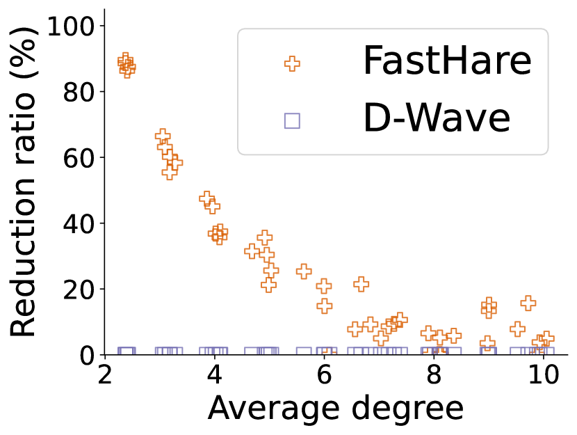
(a) Erdos-Renyi networks

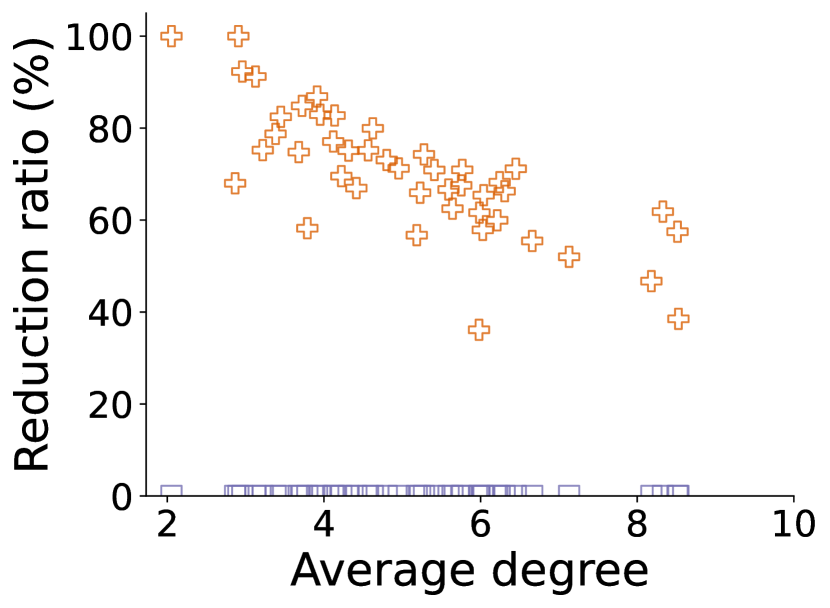
(b) Scale-free networks

Figure 4: Reduction ratio on physical qubits (the higher is better). FastHare provides significant reduction on instances of different sizes with more reduction towards sparser instances. The implemented reduction in D-Wave’s SDK offers no reduction for any instances.

Problem	#tests	#nodes	Deg.	Avg. processing time		#reducible instances		Reduction ratio
								Logical qubits		Physical qubits
				FastHare	D-Wave	FastHare	D-Wave	FastHare	D-Wave	FastHare	D-Wave
Gset [34]	17	5k-20k	2-12	0.0s	0.1s	5	3	6% (19%)	0% (2%)	NA (NA)	NA (NA)
Beasley [35]	60	0k-3k	6-250	0.0s	0.1s	20	3	8% (24%)	0% (2%)	10% (31%)	1% (4%)
Culberson [36]	108	1k-5k	4-2,927	0.1s	0.1s	57	0	8% (15%)	0% (0%)	28% (31%)	0% (0%)
Imgseg [37]	100	1k-28k	2-5	0.1s	0.2s	100	0	79% (79%)	0% (0%)	92% (92%)	0% (0%)
Others	3,111	0k-38k	1-6,965	0.3s	0.5s	1,302	296	21% (50%)	8% (82%)	35% (62%)	10% (84%)
Overall	3,396	0k-38k	1-6,965	0.3s	0.5s	1,484	302	22% (51%)	7% (81%)	36% (62%)	10% (84%)

TABLE I: Comparison on real world problems. Here, we can only embed $2,031$ instances with in an hour. The reduction ratio of physical qubits is reported based on those instances.

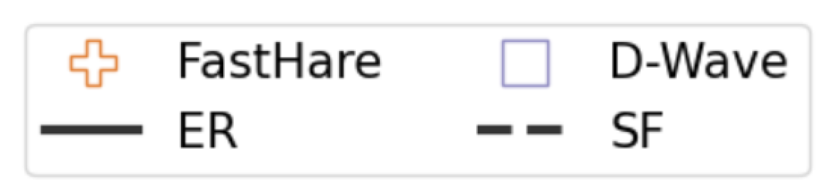
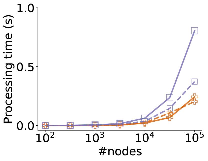
(a) Varying network size

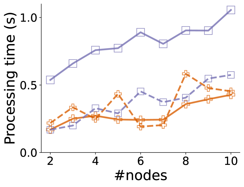
(b) Varying network density

Figure 5: Processing time in seconds on Erdos-Renyi (ER) networks, marked with solid lines, and scale-free (SF) networks, marked with dashed lines.

Reduction ratio. In Fig. 4, we show the reduction ratio on physical qubits for FastHare and D-wave. The roof duality implemented in D-Wave’s SDK offers no reduction for any instances. In contrast, FastHare can reduce all instances with the average reduction ratios on Erdos-Renyi and scale-free networks of $29\%$ and $67\%$, respectively.

The reduction ratio gets lower quickly when the average degree increases. It suggests dense Ising Hamiltonians are generally harder to reduce. In addition, the instances with Erdos-Renyi topology are much harder to reduce comparing to the ones with scale-free topology. This suggests that random Hamiltonian with Erdos-Renyi topology of high degree contain less ‘redundant’ information and, thus, can be used as hard benchmark instances for quantum solvers.

Processing time. Based on Fig. 5, the processing time of FastHare is several folds faster than D-Wave’s. For example, on the largest Erdos-Renyi network with the number of nodes $n=100,000$, the running time of FastHare and D-Wave are $0.2$s and $0.8$s, respectively. Nevertheless, in terms of processing time, both roof duality implemented in D-Wave and FastHare are highly efficient in preprocessing Hamiltonian before mapping to the QPU.

V-C Benchmark on MQLib instances

Our experiments on MQLib [32] is shown in Table I. The results indicate a significant reduction by FastHare algorithm. FastHare outperforms D-Wave in the reduction ratio. It can reduce $1,484$ out of $3,396$ instances, i.e., about 5 times more than that of D-Wave’s roof duality. The average reduction ratio in terms of logical and physical qubits among the reducible instances are $51\%$ and $62\%$, respectively. It suggest a significant qubit savings as a 62% reduction mean we can solve instances that require 2.5 times more qubits than the current limit on the state-of-the-art quantum annealers.

V-D Reducibility prediction

We investigate 70 metrics that are provided in the MQLib to see which characteristics affect the reducibility of the instances. We rank the metrics based on the Pearson correlation coefficient [39] with the reduction ratio. Top $5$ characteristics with the highest correlation for FastHare and D-Wave are shown in Table II.

The top two metrics (log norm ev2 and log norm ev1, respectively) are all calculated from the weighted graph Laplacian matrix: the logarithm of the first and second largest eigenvalues normalized by the average node degree and the logarithm of the ratio of the two largest eigenvalues (log ev ratio). This suggests that Hamiltonian with sparse cut are easier to reduce for FastHare.

The implemented D-Wave’s roof duality seems to work well on instances with constant clustering coefficient (clust_const). This behavior requires further investigation to determine the true reason behind why D-Wave’s roof duality works very well on a few instances but cannot compress for the rest.

FastHare		D-Wave
Metrics	Corr.	Metrics	Corr.
log_norm_ev2	0.73	clust_const	0.42
log_norm_ev1	0.66	clust_log_kurtosis	-0.35
mis	0.59	clust_max	-0.27
log_ev_ratio	-0.47	weight_mean	0.25
clust_stdev	0.46	mis	0.25

TABLE II: Top 5 metrics with the highest correlation with reduction ratio.

We also use logistic regression [40] to identify the metrics that have the most effect on the reducibility of the instances. Here, we remove $12$ time related metrics and normalize the remaining metrics such that the maximum absolute value of each metric equal one. For each algorithm, we set the label of an instance to one if the algorithm can reduce that instance. After running the logistic regression, we normalize the weights of the logistic regression such that the norm two of the weight vector equal one. Table III shows the top $5$ metrics with the highest absolute weights.

FastHare		D-Wave
Metrics	Weight	Metrics	Weight
chromatic	0.33	mis	0.49
weight_log_kurtosis	0.29	weight_max	-0.39
mis	0.27	avg_neighbor_deg_mean	-0.26
avg_neighbor_deg_mean	-0.24	core_log_kurtosis	0.25
log_ev_ratio	-0.20	percent_pos	-0.23

TABLE III: Top 5 metrics that have the highest absolute weights in the logistic regression.

VI Conclusion

We propose FastHare, an algorithm to reduce the size of Ising Hamiltonian, thus, provide qubits saving for quantum annealing. The method is generic and can be applied for Ising Hamiltonian of different applications. We perform the first large-scale benchmarks to measure the reducibility in 3000+ instances from MQLib library and synthesized Hamiltonian, showing significant saving in applying Hamiltonian reduction. Importantly, the fast processing time of FastHare (averaging 0.3s) make it an inexpensive choice for preprocessing. FastHare also outperforms the roof duality reduction, implemented in D-Wave’s Ocean SDK, both in time and quality by several folds. In future, FastHare can be integrated with minor-embedding methods to balance between number of physical qubits, chain lengths, and range of the coupling strengths to further improve the performance of quantum solvers.

References

- [1] F. Arute, K. Arya, R. Babbush, D. Bacon, J. C. Bardin, R. Barends, R. Biswas, S. Boixo, F. G. Brandao, D. A. Buell et al., “Quantum supremacy using a programmable superconducting processor,” Nature, vol. 574, no. 7779, pp. 505–510, 2019.
- [2] T. Honjo, T. Sonobe, K. Inaba, T. Inagaki, T. Ikuta, Y. Yamada, T. Kazama, K. Enbutsu, T. Umeki, R. Kasahara et al., “100,000-spin coherent ising machine,” Science advances, vol. 7, no. 40, p. eabh0952, 2021.
- [3] K. Bharti, A. Cervera-Lierta, T. H. Kyaw, T. Haug, S. Alperin-Lea, A. Anand, M. Degroote, H. Heimonen, J. S. Kottmann, T. Menke et al., “Noisy intermediate-scale quantum algorithms,” Reviews of Modern Physics, vol. 94, no. 1, p. 015004, 2022.
- [4] A. Mills, C. Guinn, M. Gullans, A. Sigillito, M. Feldman, E. Nielsen, and J. Petta, “Two-qubit silicon quantum processor with operation fidelity exceeding 99%,” arXiv preprint arXiv:2111.11937, 2021.
- [5] X. Wang, C. Xiao, H. Park, J. Zhu, C. Wang, T. Taniguchi, K. Watanabe, J. Yan, D. Xiao, D. R. Gamelin et al., “Light-induced ferromagnetism in moiré superlattices,” Nature, vol. 604, no. 7906, pp. 468–473, 2022.
- [6] T. Kadowaki and H. Nishimori, “Quantum annealing in the transverse ising model,” Physical Review E, vol. 58, no. 5, p. 5355, 1998.
- [7] Y. Zhou and P. Zhang, “Noise-resilient quantum machine learning for stability assessment of power systems,” IEEE Transactions on Power Systems, 2022.
- [8] D. M. Fox, K. M. Branson, and R. C. Walker, “mrna codon optimization with quantum computers,” PloS one, vol. 16, no. 10, p. e0259101, 2021.
- [9] V. K. Mulligan, H. Melo, H. I. Merritt, S. Slocum, B. D. Weitzner, A. M. Watkins, P. D. Renfrew, C. Pelissier, P. S. Arora, and R. Bonneau, “Designing peptides on a quantum computer,” BioRxiv, p. 752485, 2020.
- [10] D. M. Fox, C. M. MacDermaid, A. M. Schreij, M. Zwierzyna, and R. C. Walker, “Rna folding using quantum computers,” PLOS Computational Biology, vol. 18, no. 4, p. e1010032, 2022.
- [11] S. Mugel, M. Abad, M. Bermejo, J. Sánchez, E. Lizaso, and R. Orús, “Hybrid quantum investment optimization with minimal holding period,” Scientific Reports, vol. 11, no. 1, pp. 1–6, 2021.
- [12] C. Grozea, R. Hans, M. Koch, C. Riehn, and A. Wolf, “Optimising rolling stock planning including maintenance with constraint programming and quantum annealing,” arXiv preprint arXiv:2109.07212, 2021.
- [13] S. Yarkoni, A. Alekseyenko, M. Streif, D. Von Dollen, F. Neukart, and T. Bäck, “Multi-car paint shop optimization with quantum annealing,” in 2021 IEEE International Conference on Quantum Computing and Engineering (QCE). IEEE, 2021, pp. 35–41.
- [14] A. Mott, J. Job, J.-R. Vlimant, D. Lidar, and M. Spiropulu, “Solving a higgs optimization problem with quantum annealing for machine learning,” Nature, vol. 550, no. 7676, pp. 375–379, 2017.
- [15] F. Neukart, G. Compostella, C. Seidel, D. Von Dollen, S. Yarkoni, and B. Parney, “Traffic flow optimization using a quantum annealer,” Frontiers in ICT, vol. 4, p. 29, 2017.
- [16] M. Kim, D. Venturelli, and K. Jamieson, “Leveraging quantum annealing for large mimo processing in centralized radio access networks,” in Proceedings of the ACM Special Interest Group on Data Communication, 2019, pp. 241–255.
- [17] “D-wave hybrid solver service: An overview,” https://www.dwavesys.com/solutions-and-products/systems/, 2020.
- [18] V. Choi, “Minor-embedding in adiabatic quantum computation: I. the parameter setting problem,” Quantum Information Processing, vol. 7, no. 5, pp. 193–209, 2008.
- [19] Z. I. Tabi, Á. Marosits, Z. Kallus, P. Vaderna, I. Gódor, and Z. Zimborás, “Evaluation of quantum annealer performance via the massive mimo problem,” IEEE Access, vol. 9, pp. 131 658–131 671, 2021.
- [20] P. L. Hammer, P. Hansen, and B. Simeone, “Roof duality, complementation and persistency in quadratic 0–1 optimization,” Mathematical programming, vol. 28, no. 2, pp. 121–155, 1984.
- [21] E. Boros, P. L. Hammer, and G. Tavares, “Preprocessing of unconstrained quadratic binary optimization,” 2006.
- [22] C. Rother, V. Kolmogorov, V. S. Lempitsky, and M. Szummer, “Optimizing binary mrfs via extended roof duality,” 2007 IEEE Conference on Computer Vision and Pattern Recognition, pp. 1–8, 2007.
- [23] J.-H. Lange, B. Andres, and P. Swoboda, “Combinatorial persistency criteria for multicut and max-cut,” in Proceedings of the IEEE/CVF Conference on Computer Vision and Pattern Recognition, 2019, pp. 6093–6102.
- [24] E. Boros and P. L. Hammer, “Pseudo-boolean optimization,” Discrete applied mathematics, vol. 123, no. 1-3, pp. 155–225, 2002.
- [25] A. Lucas, “Ising formulations of many np problems,” Frontiers in physics, p. 5, 2014.
- [26] A. B. Finnila, M. Gomez, C. Sebenik, C. Stenson, and J. D. Doll, “Quantum annealing: A new method for minimizing multidimensional functions,” Chemical physics letters, vol. 219, no. 5-6, pp. 343–348, 1994.
- [27] E. Farhi, J. Goldstone, S. Gutmann, and M. Sipser, “Quantum computation by adiabatic evolution,” arXiv preprint quant-ph/0001106, 2000.
- [28] T. Albash and D. A. Lidar, “Adiabatic quantum computation,” Reviews of Modern Physics, vol. 90, no. 1, p. 015002, 2018.
- [29] V. Choi, “Minor-embedding in adiabatic quantum computation: Ii. minor-universal graph design,” Quantum Information Processing, vol. 10, no. 3, pp. 343–353, 2011.
- [30] M. R. Garey and D. S. Johnson, Computers and Intractability; A Guide to the Theory of NP-Completeness. USA: W. H. Freeman & Co., 1990.
- [31] D. Panchenko, The sherrington-kirkpatrick model. Springer Science & Business Media, 2013.
- [32] I. Dunning, S. Gupta, and J. Silberholz, “What works best when? a systematic evaluation of heuristics for max-cut and QUBO,” INFORMS Journal on Computing, vol. 30, no. 3, 2018.
- [33] D. A. Schult, “Exploring network structure, dynamics, and function using networkx,” in In Proceedings of the 7th Python in Science Conference (SciPy. Citeseer, 2008.
- [34] “Gset.” [Online]. Available: http://web.stanford.edu/~yyye/yyye/Gset/
- [35] J. E. Beasley, “Or-library: distributing test problems by electronic mail,” Journal of the operational research society, vol. 41, no. 11, pp. 1069–1072, 1990.
- [36] J. Culberson, A. Beacham, and D. Papp, “Hiding our colors,” in CP’95 Workshop on Studying and Solving Really Hard Problems. Citeseer, 1995, pp. 31–42.
- [37] S. d. Sousa, Y. Haxhimusa, and W. G. Kropatsch, “Estimation of distribution algorithm for the max-cut problem,” in International Workshop on Graph-Based Representations in Pattern Recognition. Springer, 2013, pp. 244–253.
- [38] K. Boothby, P. Bunyk, J. Raymond, and A. Roy, “Next-generation topology of d-wave quantum processors,” arXiv preprint arXiv:2003.00133, 2020.
- [39] J. Benesty, J. Chen, Y. Huang, and I. Cohen, “Pearson correlation coefficient,” in Noise reduction in speech processing. Springer, 2009, pp. 1–4.
- [40] R. E. Wright, “Logistic regression.” 1995.