Estimating Discrete Games of Complete Information:
Bringing Logit Back in the Game

Abstract

This paper considers the estimation of discrete games of complete information without assumptions on the equilibrium selection rule, which is often viewed as computationally difficult. We propose computationally attractive approaches that avoid simulation and grid search. We show that the moment inequalities proposed by Andrews, Berry, and Jia (2004) can be expressed in terms of multinomial logit probabilities, and the corresponding identified set is convex. When actions are binary, we can characterize the sharp identified set using closed-form inequalities. We also propose a simple approach to inference. Two real-data experiments illustrate that our methodology can be several orders of magnitude faster than the existing approaches.

Keywords: Estimation of games, partial identification, complete information

JEL Codes: C13, C57, L10

1 Introduction

With the increasing access to rich data and computational capabilities, empirical analysis of game-theoretic models has become standard in economics, especially in the field of empirical industrial organization. However, estimation of games with multiple equilibria remains computationally challenging since the parameters are usually partially identified. When the model is “incomplete” à la Tamer (2003), traditional statistical approaches such as the maximum likelihood estimation are not applicable. While assumptions that “complete” the model (e.g., assuming a particular equilibrium selection mechanism or the order of moves) can lead to point-identification, ad hoc assumptions may lead to model misspecification.

A series of important works have proposed practical algorithms for estimating games with weak assumptions on equilibrium selection rules (e.g., Ciliberto and Tamer (2009), Bajari, Hong, and Ryan (2010b), Galichon and Henry (2011), Beresteanu, Molchanov, and Molinari (2011), Henry, Méango, and Queyranne (2015), Pakes, Porter, Ho, and Ishii (2015), and Koh (2022)). However, the existing methods are often costly to implement because they require a combination of (i) simulation to approximate model-implied probabilities, (ii) repeatedly solving for the equilibria at each game, and/or (iii) a grid search over the parameter space. For example, Ciliberto and Jäkel (2021), who use the Ciliberto and Tamer (2009) algorithm to study the entry game by superstar exporters, report that the estimation algorithm took a week to run.

This paper contributes to the literature on the econometric analysis of games by proposing a novel estimation algorithm that is fast and simple to implement. Our approach applies to static discrete games of complete information with finite actions and finite players. It assumes pure strategy Nash equilibrium, and makes no assumption on the equilibrium selection rule. The main innovation stems from the characterization of identifying inequalities in closed forms to avoid (i)–(iii).

Let us preview the main results. We leverage the result of Galichon and Henry (2011) that characterizes the sharp identified set using a finite set of moment inequalities. Roughly speaking, Galichon and Henry (2011) show that a candidate parameter enters the sharp identified set when the conditional choice probabilities (observed by the analyst) are dominated by the generalized likelihood functions (which represent the maximal probability of outcomes predicted by the model) at all subsets of action profiles.

We obtain a tractable identified set by taking a subset of the sharp identifying restrictions that are particularly easy to handle under certain assumptions. Specifically, rather than considering all identifying inequalities that characterize the sharp identified set, we choose a subset based on the singleton class. When each player’s payoff function is additively separable and the action-specific idiosyncratic payoff shocks independently follow the type 1 extreme value distribution, each inequality in the subset admits a closed-form expression in terms of the multinomial logit probabilities. Moreover, when the payoff functions are linear in the parameters, the corresponding identified set is convex. The identified set is equivalent to that of Andrews, Berry, and Jia (2004). However, while Andrews, Berry, and Jia (2004) use the normal distribution assumption on the latent payoff shocks and resort to simulation to approximate the generalized likelihoods, we observe that the computation can be greatly simplified when the distributional assumption is replaced with the type 1 extreme value distribution. The characterization holds regardless of the number of players and actions in so far as they are finite. Although the identified set is potentially non–sharp, it yields tractable estimation routines applicable to a large class of empirical problems.

Many empirical applications in the discrete games literature have focused on games with binary actions. In the special case where players’ actions are binary, it turns out we can express the sharp identifying restrictions using a finite number of closed-form inequalities. Our characterization of the sharp identified set for binary action games is new.

Given the closed form characterizations of (sharp or non-sharp) identifying restrictions, we propose computationally tractable approaches for estimation and inference. Determining whether a candidate parameter enters the identified set amounts to numerically evaluating closed-form expressions. To quickly find a point in the identified set or the projection intervals, we cast the problems as optimization problems that can be solved efficiently using the state-of-the-art algorithms. In our benchmark Monte Carlo experiment, we measure the time to compute the projections of the identified set and find that our strategy can be approximately one million times faster than the Ciliberto and Tamer (2009) algorithm (although the relative speed gain depends on the simulation parameters such as the number of simulation draws and the number of points used to approximate the parameter space). Finally, we also propose a simple and computationally attractive approach to constructing confidence sets for the identified sets by leveraging the key insights from Horowitz and Lee (2021); the main idea is to account for the sampling uncertainty by constructing simultaneous confidence intervals for the conditional choice probabilities.

We illustrate the usefulness of our approach using two real-data experiments. We apply our methodology to the empirical models in Kline and Tamer (2016) and Ellickson and Misra (2011) and compute the confidence set for the sharp identified set without assumptions on the equilibrium selection rule. We also incorporate unobserved market-level common payoff shocks that are publicly observable to the players but not to the analyst. We find that our approach generates results that are qualitatively similar to the original papers. Moreover, in both examples, it takes less than five minutes to obtain the final table; all computation was done without parallelization in Julia v1.6.1 on a 2020 13-inch MacBook Pro device with Apple M1 chip and 16GB memory, using solver Knitro v13.0.1 with four starting points for each optimization problem.

The main innovation of this paper is to develop a fast and simple approach that dramatically lowers the costs of estimating static games of complete information without assumptions on the equilibrium selection rule. Compared to the existing estimation algorithms such as Ciliberto and Tamer (2009) that work under general assumptions on payoff functions and distribution of latent variables, our approach obtains speed gains by imposing assumptions that are stronger but quite standard and empirically relevant. To the best of our knowledge, there is no algorithm for estimating complete information games that leverages the multinomial logit formula when the parameters are partially identified. Thus, this paper brings logit “back in the game” to speed up estimation.

The rest of the paper is organized as follows. Section 2 introduces the model and propose an identified set that is characterizable with closed-form inequalities. Section 3 specializes to games with binary actions and shows that the sharp identified set can be characterized using a finite number of closed-form inequalities. Section 4 presents computational strategies for estimation problems. Section 5 proposes a computationally tractable approach to constructing confidence sets. Section 6 shows the performance of our methodology when applied to real-world datasets. Section 7 concludes. All proofs are in Appendix A.

2 Theory

2.1 Preliminaries

Our framework follows the exposition in Galichon and Henry (2011) (henceforth GH). An econometric model is specified as

$$y\in G\left(\varepsilon|x;\theta\right).$$

$y\in\mathcal{Y}$ denotes outcome variables; $x\in\mathcal{X}$ denotes a vector of exogenous covariates observable to the researcher; $\varepsilon\in\mathcal{E}$ is a vector of latent variables, unobserved by the researcher, whose distribution is denoted as $\nu\left(\cdot|x;\theta\right)$; $\theta\in\Theta\subseteq\mathbb{R}^{d}$ denotes a vector of structural parameters that the econometrician wants to identify; $G:\mathcal{E}\times\mathcal{X}\times\Theta\rightrightarrows\mathcal{Y}$ represents an incomplete econometric model that specifies the set of possible outcomes given state $\left(x,\varepsilon\right)$ and parameter $\theta$. The econometrician observes $\left\{y_{m},x_{m}\right\}_{m=1}^{n}$ where $m$ indexes independent observations and $n$ is the total number of observations. We assume that as $n\to\infty$, the econometrician can identify the conditional choice probabilities (CCP) $\phi\equiv\left\{\phi\left(y|x\right)\right\}_{y\in\mathcal{Y},x\in\mathcal{X}}$ where each $\phi\left(y|x\right)$ denotes the probability of observing outcome $y\in\mathcal{Y}$ given covariates $x\in\mathcal{X}$.

Static Discrete Games of Complete Information

Let us specialize to static discrete games of complete information with finite players and finite actions. We assume observations come from independent markets. Let $i\in\mathcal{I}=\left\{1,...,I\right\}$ index the players. Player $i$’s action is denoted by $y_{i}\in\mathcal{Y}_{i}$ where $\mathcal{Y}_{i}$ is finite. An action profile is denoted by $y=\left(y_{1},y_{2},...,y_{I}\right)\in\mathcal{Y}\equiv\times_{i=1}^{I}\mathcal{Y}_{i}$, and we use the convention $y=\left(y_{i},y_{-i}\right)$ where $y_{-i}=\left(y_{1},...,y_{i-1},y_{i+1},...,y_{I}\right)$ denotes the actions of $i$’s opponents. Covariates are denoted by a vector $x\in\mathcal{X}$ where $\mathcal{X}$ is assumed to be finite. Finally, $\varepsilon\in\mathcal{E}$ captures all latent variables that enter the players’ payoff functions. As is standard in the empirical literature, we assume that $\varepsilon=\left(\varepsilon_{1},...,\varepsilon_{I}\right)$ where each $\varepsilon_{i}$ enters only $i$’s payoff. Each player’s payoff functions are given by $u_{i}:\mathcal{Y}\times\mathcal{X}\times\mathcal{E}_{i}\times\Theta\to\mathbb{R}$. The game is common knowledge to the players.

We assume that information is complete, i.e., the realized state of the world $\left(x,\varepsilon\right)$ is common knowledge to the players. The solution concept is pure strategy Nash equilibrium. Thus, $G\left(\varepsilon|x;\theta\right)\subseteq\mathcal{Y}$ describes the set of all complete information pure strategy Nash equilibrium action profiles at state $\left(x,\varepsilon\right)$ and parameter $\theta$.

Throughout the paper, we assume that the CCP $\phi$ is generated by a mixture of pure strategy Nash equilibria at some true parameter vector with arbitrary equilibrium selection rule. The econometrician’s objective is to estimate the parameters of the model without assumptions on the equilibrium selection rule. The parameters are typically partially identified.

We use a two-player entry game as a running example throughout the paper. The empirical models in Section 6 are extensions of the example. Section C considers a numerical example with two players, each of whom can choose from three actions.

Example 1 (Two-player entry game).

There are two players $i=1,2$. Each player $i$ can choose to $y_{i}=1$ (enter) or $y_{i}=0$ (stay out), so $\mathcal{Y}_{i}=\left\{0,1\right\}$. The set of possible outcomes is $\mathcal{Y}=\left\{\left(0,0\right),\left(0,1\right),\left(1,0\right),\left(1,1\right)\right\}$. Let $\varepsilon_{i}=\left(\varepsilon_{i}\left(0\right),\varepsilon_{i}\left(1\right)\right)\in\mathbb{R}^{2}$ describes action-specific payoff shocks. After the players observe the realized state of the world $\left(x,\varepsilon\right)$, they choose actions simultaneously. Each player $i$ receives the following payoff:

$$u_{i}\left(y_{i},y_{-i},x,\varepsilon_{i};\theta\right)=\begin{cases}\beta_{i}^{T}x_{i}+\Delta_{i}y_{j}+\varepsilon_{i}\left(1\right)&\text{if }y_{i}=1\\ \varepsilon_{i}\left(0\right)&\text{if }y_{i}=0\end{cases}$$

The parameter $\Delta_{i}\in\mathbb{R}$ is the “competition effect” parameter that captures how much the opponent’s presence increases or decreases $i$’s profit when $i$ is operating in the market. The parameters to be estimated are $\theta=\left(\beta_{1},\beta_{2},\Delta_{1},\Delta_{2}\right)$.

When the solution concept is pure strategy Nash equilibrium, $y_{i}=1$ if and only if $x_{i}^{T}\beta_{i}+\Delta_{i}y_{j}+\xi_{i}\geq 0$ where $\xi_{i}\equiv\varepsilon_{i}\left(1\right)-\varepsilon_{i}\left(0\right)$. For expositional simplicity, we assume $\Delta_{i}\leq 0$ for $i=1,2$, implying that the set of equilibria at each realization of $\left(\xi_{1},\xi_{2}\right)$ are given by Figure 1 (see, e.g., Tamer (2003), Ciliberto and Tamer (2009), or Aradillas-López (2020)). The $\xi$’s at the center region admits two outcomes, $\left(0,1\right)$ and $\left(1,0\right)$, as Nash equilibria, i.e., $G\left(\xi|x;\theta\right)=\left\{\left(0,1\right),\left(1,0\right)\right\}$ if $\xi\in\times_{i=1}^{2}\left(-x_{i}^{T}\beta_{i},-x_{i}^{T}\beta_{i}-\Delta_{i}\right)$. The other region admits a unique equilibrium. $\blacksquare$

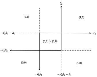
Figure 1: Structure of equilibria in a two-player entry game when $\Delta_{i}\leq 0$

Galichon and Henry (2011)’s Characterization of the Sharp Identified Set

We build on GH’s characterization of the sharp identified set. For clarity, let us review their main findings. For any subset $A\subseteq\mathcal{Y}$, let $G^{-1}\left(A|x;\theta\right):=\left\{\varepsilon\in\mathcal{E}:G\left(\varepsilon|x;\theta\right)\cap A\neq\emptyset\right\}$ which represents a collection of all state $\varepsilon$ at which an outcome in $A$ is a possible equilibrium. Define the generalized likelihood function (also called Choquet capacity) as $\mathcal{L}\left(A|x;\theta\right)=\nu\left(G^{-1}\left(A|x;\theta\right)|x;\theta\right)$, which can be interpreted as the maximal probability of observing some outcome in $A$.

Theorem 1 of GH states that the sharp identified set, denoted $\Theta_{I}^{sharp}$, is a collection of $\theta$’s such that the true conditional choice probabilities are dominated by the generalized likelihood for every possible subset $A$ of $\mathcal{Y}$ (or, more formally, true conditional choice probabilities lie in the core of the Choquet capacity $\mathcal{L}$).

Theorem 1 (Galichon and Henry (2011)).

The sharp identified set $\Theta_{I}^{sharp}$ is equal to the set of parameters such that the true distribution of the observable variables lies in the core of the generalized likelihood predicted by the model. Hence,

$$\Theta_{I}^{sharp}=\left\{\theta\in\Theta:\ \text{for every subset $A$ of $\mathcal{Y}$, }\sum_{y\in A}\phi\left(y|x\right)\leq\mathcal{L}\left(A|x;\theta\right),\ x-\text{a.s.}\right\}.$$ (1)

The significance of Theorem 1 is that it provides an operational characterization of the sharp identified set: for any candidate $\theta$, one can determine whether $\theta\in\Theta_{I}^{\text{sharp}}$ using a finite number of moment inequalities without resorting to an (unknown) equilibrium selection rule, which is an infinite-dimensional nuisance parameter.

However, numerically computing $\Theta_{I}^{sharp}$ using (1) can be costly. Existing works approximate each $\mathcal{L}\left(A|x;\theta\right)$ by simulating a large number of $\varepsilon$’s and computing $G\left(\varepsilon|x;\theta\right)$ at each draw by solving for all equilibria. The simulation procedure is repeated at a large number of points in the parameter space in order to numerically approximate the identified set. High computational burden due to a a combination of simulation and grid search is a common feature of the existing approaches (e.g., Ciliberto and Tamer (2009), Bajari, Hong, and Ryan (2010b), Beresteanu, Molchanov, and Molinari (2011), Galichon and Henry (2011), and Henry, Méango, and Queyranne (2015)).

2.2 A Tractable Identified Set

We propose an (non-sharp) identified set that is highly tractable. The key idea is to use, out of all inequalities in (1), only those based on the singleton class (subsets of $\mathcal{Y}$ that are singletons). When combined with the assumption that the payoff shocks are additive and independently follow the type 1 extreme value distribution, we are able to express the inequalities in closed form. The identifying restrictions are identical to those used by Andrews, Berry, and Jia (2004) (henceforth ABJ) who use the fact that $\phi\left(y|x\right)$ cannot be larger than the probability that $y$ is a possible equilibrium outcome to generate moment inequalities.

Assumption 1.

Each player’s payoff function takes an additively separable form

$$u_{i}\left(y_{i},y_{-i},x,\varepsilon_{i};\theta\right)=v_{i}\left(y_{i},y_{-i},x;\theta\right)+\varepsilon_{i}\left(y_{i}\right).$$

Each $\varepsilon_{i}\left(y_{i}\right)\in\mathbb{R}$ independently follows the type 1 extreme value distribution.

Assumption 1 is quite standard. Note that the assumption implies $\varepsilon=\left(\varepsilon_{1},...,\varepsilon_{I}\right)$ and that $\varepsilon_{i}=\left(\varepsilon_{i}\left(y_{i}\right)\right)_{y_{i}\in\mathcal{Y}_{i}}$, i.e., the latent variable of the model is a vector of player specific shocks, each of which is a vector of action-specific shocks.

We claim that, under Assumption 1, the generalized likelihood functions $\mathcal{L}\left(A|x;\theta\right)$ admit closed-form expressions when $A$ is a singleton. Let us slightly abuse the notation and write $\mathcal{L}\left(y|x;\theta\right)\equiv\mathcal{L}\left(\left\{y\right\}|x;\theta\right)$. When we restrict attention to the singleton class, we obtain an outer set defined as

$$\Theta_{I}^{ABJ}:=\left\{\theta\in\Theta:\ \phi\left(y|x\right)\leq\mathcal{L}\left(y|x;\theta\right)\quad\forall y\in\mathcal{Y},x\in\mathcal{X}\right\}.$$ (2)

Clearly $\Theta_{I}^{sharp}\subseteq\Theta_{I}^{ABJ}$. Although $\Theta_{I}^{ABJ}$ does not exploit all identifying contents of the model, the following result shows that it is easy to compute the set.

Theorem 2.

Under Assumption 1, the identified set in (2) can be rewritten as

$$\Theta_{I}^{ABJ}=\left\{\theta\in\Theta:\ \phi\left(y|x\right)\leq\prod_{i=1}^{I}\frac{\exp\left(v_{i}\left(y,x;\theta\right)\right)}{\sum_{y_{i}^{\prime}\in\mathcal{Y}_{i}}\exp\left(v_{i}\left(y_{i}^{\prime},y_{-i},x;\theta\right)\right)},\quad\forall y\in\mathcal{Y},x\in\mathcal{X}\right\}.$$ (3)

Let us explain the intuition. Recall that $\mathcal{L}\left(y|x;\theta\right)\equiv\text{Pr}\left(\varepsilon\in G^{-1}\left(y|x;\theta\right)\right)$. Since $\varepsilon_{i}$ only enter’s agent $i$’s payoff, we have $\varepsilon\in G^{-1}\left(y|x;\theta\right)$ if and only if $\varepsilon_{i}\in M_{i}\left(y_{i}|y_{-i},x;\theta\right)$ for all $i=1,...,I$ where

$$M_{i}\left(y_{i}|y_{-i},x;\theta\right)\equiv\left\{\varepsilon_{i}:\ v_{i}\left(y_{i},y_{-i},x;\theta\right)+\varepsilon_{i}\left(y_{i}\right)\geq v_{i}\left(y_{i}^{\prime},y_{-i},x;\theta\right)+\varepsilon_{i}\left(y_{i}^{\prime}\right)\right\}.$$

So $\mathcal{L}\left(y|x;\theta\right)=\text{Pr}\left(\times_{i=1}^{I}M_{i}\left(y_{i}|y_{-i},x;\theta\right)\right)=\prod_{i=1}^{I}\text{Pr}\left(M_{i}\left(y_{i}|y_{-i},x;\theta\right)\right)$, where $\times_{i=1}^{I}$ denotes the Cartesian product, and the last equality follows from the independence assumption. But the probability of $M_{i}\left(y_{i}|y_{-i},x;\theta\right)$ is simply the probability that $y_{i}$ is optimal to agent $i$ who takes $y_{-i}$ as exogenous. Under the type 1 extreme value distribution assumption, $\text{Pr}\left(M_{i}\left(y_{i}|y_{-i},x;\theta\right)\right)$ takes the multinomial logit form.

Suppose that $\phi$ is identified from the data and that $v_{i}\left(y,x;\theta\right)$ is a closed-form function of $\theta$. Theorem 2 shows that, for each candidate $\theta$, determining whether $\theta\in\Theta_{I}^{ABJ}$ can be done using closed-form inequalities. The researcher does not need to simulate $\varepsilon$’s nor solve for the equilibrium even once. Checking whether $\theta\in\Theta_{I}^{ABJ}$ is extremely easy. Section 4 shows that, if $v_{i}\left(y,x;\theta\right)$ is also linear in $\theta$, the projection of $\Theta_{I}^{ABJ}$ in a given direction $p\in\mathbb{R}^{\dim\left(\theta\right)}$ can be obtained by solving a single convex program.

Example.

(Example 1 continued) In Figure 2, we show $G^{-1}\left(y|x;\theta\right)$ for each $y\in\mathcal{Y}$ in the $\left(\xi_{1},\xi_{2}\right)$-space. For example, Figure 2-(a) shows the set of $\left(\xi_{1},\xi_{2}\right)$ that supports the outcome $y=\left(0,0\right)$ (both players do not enter) as a possible Nash equilibrium. Similarly, Figure 2-(b) represents the set of $\left(\xi_{1},\xi_{2}\right)$ which supports $\left(y_{1},y_{2}\right)=\left(0,1\right)$ as a possible Nash equilibrium. A common feature of $G^{-1}\left(y|x;\theta\right)$ for each $y$ is that they are rectangles whose probabilities are extremely easy to compute when each $\xi_{i}$ follows the standard logistic distribution.

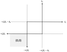
Figure 2: Computing probability of rectangles

(a) $G^{-1}\left(\left(0,0\right)|x;\theta\right)$

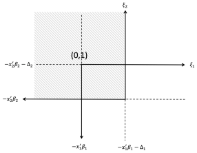
(b) $G^{-1}\left(\left(0,1\right)|x;\theta\right)$

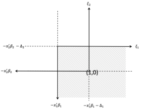
(c) $G^{-1}\left(\left(1,0\right)|x;\theta\right)$

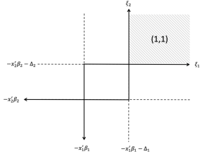
(d) $G^{-1}\left(\left(1,1\right)|x;\theta\right)$

According to (3), $\theta=\left(\beta_{1},\beta_{2},\Delta_{1},\Delta_{2}\right)\in\Theta_{I}^{ABJ}$ if and only if for all $x\in\mathcal{X}$,

$$\phi\left(0,0|x\right) \leq F\left(-\beta_{1}^{T}x_{1}\right)F\left(-\beta_{2}^{T}x_{2}\right)$$

$$\phi\left(1,1|x\right) \leq\left(1-F\left(-\beta_{1}^{T}x_{1}-\Delta_{1}\right)\right)\left(1-F\left(-\beta_{2}^{T}x_{2}-\Delta_{2}\right)\right)$$

$$\phi\left(1,0|x\right) \leq\left(1-F\left(-\beta_{1}^{T}x_{1}\right)\right)F\left(-\beta_{2}^{T}x_{2}-\Delta_{2}\right)$$

$$\phi\left(0,1|x\right) \leq F\left(-\beta_{1}^{T}x_{1}-\Delta_{1}\right)\left(1-F\left(-\beta_{2}^{T}x_{2}\right)\right)$$

where $F\left(z\right)\equiv 1/\left(1+e^{-z}\right)$ is the cumulative distribution function of the standard logistic random variable. The above inequalities are intuitive: conditional on $x$, the probability of outcome $y$ cannot be larger the maximal probability of $y$ predicted by the model. $\blacksquare$

Comparison to the Sharp Identified Set

Using an outer set may result in unnecessary loss of information compared to the sharp set, which exhausts all information available to the researcher. However, at the minimum, the ABJ-identified set can help quickly rule out parameters that are rejected by the model. It is natural to ask how much loss of identifying power the outer set entails. We use a numerical example to examine this question.

Let us continue with Example 1. Set $\theta=\left(\beta_{1},\beta_{2},\Delta_{1},\Delta_{2}\right)=\left(0.0,0.0,-0.5,-0.5\right)$. Assume that the equilibrium selection rule is symmetric. The model yields the choice probability vector $\left(\phi_{00},\phi_{10},\phi_{01},\phi_{11}\right)=\left(0.250,0.304,0.304,0.142\right)$.

Table 1: Comparison of the projected identified sets

			Sharp		ABJ
		$\beta_{1}$	$[-0.214,0.193]$		$[-0.217,0.196]$
		$\beta_{2}$	$[-0.214,0.193]$		$[-0.217,0.196]$
		$\Delta_{1}$	$[-0.936,-0.014]$		$[-0.945,-0.005]$
		$\Delta_{2}$	$[-0.936,-0.014]$		$[-0.945,-0.005]$

Table 1 reports the projection intervals of $\Theta_{I}^{sharp}$ and $\Theta_{I}^{ABJ}$. The four parameters are estimated jointly without using the knowledge that $\beta_{1}=\beta_{2}$ and $\Delta_{1}=\Delta_{2}$. Comparing the intervals reveals that the outer set generates projection intervals that are essentially identical to those of the sharp set.

Convexity of the ABJ Set

Theorem 2 is quite general in that it makes no assumption on the structure of $v_{i}\left(y,x;\theta\right)$. It turns out that if $v_{i}\left(y,x;\theta\right)$ is linear in $\theta$, we can facilitate computation even further because $\Theta_{I}^{ABJ}$ becomes a convex set described by a finite set of inequalities.

Assumption 2.

For each $y\in\mathcal{Y}$ and $x\in\mathcal{X}$, $v_{i}\left(y,x;\theta\right)$ is linear in $\theta$.

Lemma 1.

Under Assumptions 1 and 2, for each $y\in\mathcal{Y}$ and $x\in\mathcal{X}$, $\mathcal{L}\left(y|x;\theta\right)$ is log-concave in $\theta$.

Let us rearrange the inequalities (3) so that we can leverage Assumption 2. Rewrite the inequalities in (3) as

$$\phi\left(y|x\right)\leq\mathcal{L}\left(y|x;\theta\right)\quad\forall y\in\mathcal{Y},x\in\mathcal{X}$$ (4)

$$\Leftrightarrow g_{y,x}^{ABJ}\left(\theta;\phi\right)\leq 0,\quad\forall y\in\mathcal{Y},x\in\mathcal{X}$$ (5)

where

$$g_{y,x}^{ABJ}\left(\theta;\phi\right) :=\log\left(\phi\left(y|x\right)\right)-\log\left(\mathcal{L}\left(y|x;\theta\right)\right)$$ (6)

$$=\log\left(\phi\left(y|x\right)\right)-\sum_{i=1}^{I}\left\{v_{i}\left(y,x;\theta\right)-\log\left(\sum_{y_{i}^{\prime}\in\mathcal{Y}_{i}}\exp\left(v_{i}\left(y_{i}^{\prime},y_{-i},x;\theta\right)\right)\right)\right\}$$

is obtained by taking logs on both sides of (4) and rearranging the terms. Thus, we have

$$\Theta_{I}^{ABJ}\equiv\left\{\theta\in\Theta:\ g_{y,x}^{ABJ}\left(\theta;\phi\right)\leq 0,\quad\forall y\in\mathcal{Y},x\in\mathcal{X}\right\}.$$ (7)

Since $\phi$ is a constant and $\mathcal{L}\left(y|x,\theta\right)$ is log-concave, $g_{y,x}^{ABJ}\left(\theta;\phi\right)$ is convex in $\theta$, which in turn implies that $\Theta_{I}^{ABJ}$ is convex.

Theorem 3.

Under Assumptions 1 and 2, $\Theta_{I}^{ABJ}$ is convex.

Example.

(Example 1 continued) Let us continue to consider the example considered in Section 2.2, but now suppose that the researcher knows $\beta_{i}=0$ for $i=1,2$ and wants to identify $\Delta_{i}$ for $i=1,2$. Figure 3 plots $\Theta_{I}^{ABJ}$ in blue, $\Theta_{I}^{sharp}$ in red, and the location of the true parameter is shown in a star. Clearly, we have $\theta_{0}\in\Theta_{I}^{sharp}\subseteq\Theta_{I}^{ABJ}$, and $\Theta_{I}^{ABJ}$ is convex as implied by Theorem 3. While $\Theta_{I}^{ABJ}$ is much wider than $\Theta_{I}^{sharp}$, they deliver essentially identical projection intervals in each dimension. $\blacksquare$

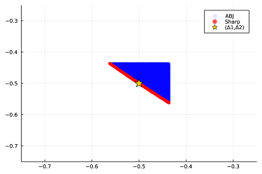
Figure 3: Convex identified set

2.3 Lower Bounds Using Probability of Strictly Dominant Strategies

In the previous section, we have characterized easy-to-use upper bounds on $\phi$. We can also find easy-to-use lower-bounds on each $\phi$ based on the probabilities of dominant actions.

The probability that $y_{i}$ is a strictly dominant strategy for player $i$ can be characterized in closed-form as follows.

Theorem 4.

Let Assumption 1 hold. Let $x\in\mathcal{X}$ and $\theta\in\Theta$ be given. The probability that an action $y_{i}\in\mathcal{Y}_{i}$ is a strictly dominant strategy for player $i$ is given by

$$\frac{1}{\sum_{\tilde{y}_{i}\in\mathcal{Y}_{i}}\exp\left(-h_{i}\left(y_{i},\tilde{y}_{i},x;\theta\right)\right)}$$

where $h_{i}\left(y_{i},\tilde{y}_{i},x;\theta\right)\equiv\min_{y_{-i}\in\mathcal{Y}_{-i}}\left\{v_{i}\left(y_{i},y_{-i},x;\theta\right)-v_{i}\left(\tilde{y}_{i},y_{-i},x;\theta\right)\right\}$.

Since player $i$’s probability of playing $y_{i}$ cannot be lower than the probability that $y_{i}$ is a strictly dominant strategy, Theorem 4 implies the following lower bounds on the conditional choice probabilities:

$$\phi\left(y|x\right)\geq\prod_{i=1}^{I}\frac{1}{\sum_{\tilde{y}_{i}\in\mathcal{Y}_{i}}\exp\left(-h_{i}\left(y_{i},\tilde{y}_{i},x;\theta\right)\right)},\quad\forall y\in\mathcal{Y},x\in\mathcal{X}.$$ (8)

Remark 1.

Combining the ABJ upper bounds (2) and the lower bounds (8) for the conditional choice probabilities defines an (non-sharp) identified set for the parameters. The identified set is weakly larger than the identified set proposed by Ciliberto and Tamer (2009) who also combine model-implied upper bounds and lower bounds to generate identifying restrictions. The upper bounds are identical across the two identified sets. However, the lower bounds (8) are weakly lower than the Ciliberto and Tamer (2009) lower bounds that find the probability of an outcome being a unique equilibrium. The reason is simply that when each action in an action profile is a dominant action, the action profile must be a unique pure strategy Nash equilibrium, but not vice versa. $\blacksquare$

Example.

(Example 1 continued) We have

$$h_{i}\left(y_{i},\tilde{y}_{i},x;\theta\right) =\min_{y_{j}}\left(y_{i}-\tilde{y}_{i}\right)\left(\beta_{i}^{T}x_{i}+\Delta_{i}y_{j}\right).$$

Given the assumption that $\Delta_{i}\leq 0$, we can obtain

$$\frac{1}{\sum_{\tilde{y}_{i}\in\mathcal{Y}_{i}}\exp\left(-h_{i}\left(y_{i},\tilde{y}_{i},x;\theta\right)\right)}=\begin{cases}F\left(-\beta_{i}^{T}x_{i}\right)&\text{if }y_{i}=0\\ 1-F\left(-\beta_{i}^{T}x_{i}-\Delta_{i}\right)&\text{if }y_{i}=1\end{cases}.$$

Thus, we obtain the following lower bounds on the conditional choice probabilities

$$F\left(-\beta_{1}^{T}x_{1}\right)F\left(-\beta_{2}^{T}x_{2}\right) \leq\phi\left(0,0|x\right)$$

$$\left(1-F\left(-\beta_{1}^{T}x_{1}-\Delta_{1}\right)\right)\left(1-F\left(-\beta_{2}^{T}x_{2}-\Delta_{2}\right)\right) \leq\phi\left(1,1|x\right)$$

$$\left(1-F\left(-\beta_{1}^{T}x_{1}-\Delta_{1}\right)\right)F\left(-\beta_{2}^{T}x_{2}\right) \leq\phi\left(1,0|x\right)$$

$$F\left(-\beta_{1}^{T}x_{1}\right)\left(1-F\left(-\beta_{2}^{T}x_{2}-\Delta_{2}\right)\right) \leq\phi\left(0,1|x\right).$$

$\blacksquare$

2.4 Unobserved Heterogeneity

In empirical applications, it is important to incorporate market-level characteristics that are commonly observed by the players but not by the researcher. A common approach is to make a parametric assumption on the market-level shocks (see, e.g., Aguirregabiria and Mira (2007), Ciliberto and Tamer (2009), Ciliberto et al. (2016), and Ciliberto and Jäkel (2021)). It is straightforward to accommodate such an assumption into our framework.

Let $\omega\in\Omega$ be market-level characteristics that are common knowledge to the players but unobservable to the researcher. Let us augment the payoff function to accommodate $\omega$ and write $u_{i}\left(y,x,\omega,\varepsilon;\theta\right)=v_{i}\left(y,x,\omega;\theta\right)+\varepsilon_{i}\left(y_{i}\right)$. Suppose $\omega$ is drawn i.i.d. from a distribution $H$ whose parameter also enters $\theta$.

Suppose the model implies inequalities of the form

$$L\left(A,x,\omega;\theta\right)\leq q\left(A|x,\omega\right)\leq U\left(A,x,\omega;\theta\right),\quad\forall A\in\mathcal{A},x\in\mathcal{X},\omega\in\Omega$$

where $\mathcal{A}\subseteq 2^{\mathcal{Y}}$, $q\left(A|x,\omega\right)\equiv\sum_{y\in A}q\left(y|x,\omega\right)$, $q\left(y|x,\omega\right)$ is the true CCP generated by the model, and $L\left(y,x,\omega;\theta\right)$ and $U\left(y,x,\omega;\theta\right)$ are available in closed forms. Since the researcher does not observe $q\left(A|x,\omega\right)$, but observes $\phi\left(A|x\right)\equiv\int q\left(A|x,\omega\right)dH\left(\omega;\theta\right)$, the identifying restrictions are obtained by integrating out $\omega$:

$$\int L\left(A,x,\omega;\theta\right)dH\left(\omega;\theta\right)\leq\phi\left(A|x\right)\leq\int U\left(y,x,\omega;\theta\right)dH\left(\omega;\theta\right),\quad\forall A\in\mathcal{A},x\in\mathcal{X}.$$

The moment inequalities can be approximated by using simulation:

$$\frac{1}{S}\sum_{s=1}^{S}L\left(A,x,\omega^{s};\theta\right)\leq\phi\left(A|x\right)\leq\frac{1}{S}\sum_{s=1}^{S}U\left(A,x,\omega^{s};\theta\right),\quad\forall A\in\mathcal{A},x\in\mathcal{X}.$$

Example.

(Example 1 continued) In a two-player entry game, let $v_{i}\left(y_{i},y_{-i},x,\omega;\theta\right)=y_{i}\left(\beta_{i}^{T}x_{i}+\Delta_{i}y_{j}+\sigma_{\omega}\omega\right)$ and assume that $\omega\overset{iid}{\sim}Logistic\left(0,1\right)$. The parameters to estimate are $\theta=\left(\beta_{1},\beta_{2},\Delta_{1},\Delta_{2},\sigma_{\omega}\right)$. The identifying restrictions implied by the ABJ inequalities yield

$$\phi\left(y|x\right)\leq\int\mathcal{L}\left(y|x,\omega;\theta\right)dH\left(\omega\right),\quad\forall y\in\mathcal{Y},x\in\mathcal{X}$$

where

$$\mathcal{L}\left(y|x,\omega\right)=\prod_{i=1}^{I}\frac{\exp\left(v_{i}\left(y,x,\omega;\theta\right)\right)}{\sum_{y_{i}^{\prime}\in\mathcal{Y}}\exp\left(v_{i}\left(y_{i}^{\prime},y_{-i},x,\omega;\theta\right)\right)}.$$

$\blacksquare$

3 Games with Binary Actions

The previous section has provided easy-to-use identifying restrictions that are agnostic about the number of actions available to the players. When players’ actions are binary, we obtain a stronger result: we are able to characterize the sharp identified set using a finite set of closed-form inequalities. Our characterization of the sharp identified set for games with binary actions is new.

Assumption 3.

For each player $i=1,...,I$, the action set is $\mathcal{Y}_{i}=\left\{0,1\right\}$. The payoff function is $u_{i}\left(y_{i},y_{-i},x,\xi_{i};\theta\right)=y_{i}\left(w_{i}\left(y_{-i},x;\theta\right)+\xi_{i}\right)$ where each $\xi_{i}$ is i.i.d. with cumulative distribution function $F$.

Assumption 3 normalizes $i$’s payoff from $y_{i}=0$ (“staying out”) to zero. The payoff from $y_{i}=1$ (“staying in”) is $w_{i}\left(y_{-i},x;\theta\right)+\xi_{i}$. In practice, it will be convenient to assume that each $\xi_{i}$ follows a standard logistic distribution since $F\left(c\right)\equiv\text{Pr}\left(\xi_{i}\leq c\right)$ is available in closed form.

We prove the following claim.

Claim 1.

Under Assumption 3, for any $A\subseteq\mathcal{Y}$, $x\in\mathcal{X}$, and $\theta\in\Theta$, $\mathcal{L}\left(A|x;\theta\right)$ admits a closed-form expression.

In the previous section, we showed that each $\mathcal{L}\left(A|x;\theta\right)$ admits a closed-form expression if $A$ is a singleton. Claim 1 says that, if actions are binary, $\mathcal{L}\left(A|x;\theta\right)$ admits a closed-form expression for any $A\in 2^{\mathcal{Y}}$ regardless of its cardinality.

Let us derive the expressions for each $\mathcal{L}\left(A|x;\theta\right)$. First, note that we can rewrite the generalized likelihood function as

$$\mathcal{L}\left(A|x;\theta\right) \equiv\text{Pr}\left(\left\{\xi:\ G\left(\xi|x;\theta\right)\cap A\neq\emptyset\right\}\right)=\text{Pr}\left(\bigcup_{\tilde{y}\in A}G^{-1}\left(\left\{\tilde{y}\right\}|x;\theta\right)\right).$$

Next, define

$$\mathcal{R}\left(A|x;\theta\right) \equiv\text{Pr}\left(\left\{\xi:\ A\subseteq G\left(\xi|x;\theta\right)\right\}\right)=\text{Pr}\left(\bigcap_{\tilde{y}\in A}G^{-1}\left(\left\{\tilde{y}\right\}|x;\theta\right)\right).$$

In words, $\mathcal{L}\left(A|x;\theta\right)$ measures the probability over the $\xi$’s that support some outcome in $A$ as a possible equilibrium whereas $\mathcal{R}\left(A|x;\theta\right)$ measures the probability over the $\xi$’s that support all outcomes in $A$ as (a subset of) possible equilibria. Observe that (i) $\mathcal{L}\left(A|x;\theta\right)$ represents the probability of a union of events whereas $\mathcal{R}\left(A|x;\theta\right)$ represents the probability of an intersection of events, and (ii) $\mathcal{L}\left(A|x;\theta\right)=\mathcal{R}\left(A|x;\theta\right)$ if $A$ is a singleton.

Example.

(Example 1 continued) In the running example, we have

$$\mathcal{L}\left(\left\{\left(0,1\right)\right\}|x;\theta\right)=\mathcal{R}\left(\left\{\left(0,1\right)\right\}|x;\theta\right)=\text{Pr}\left(\xi_{1}\leq-x_{1}^{T}\beta_{1}-\Delta_{1},\xi_{2}>-x_{2}^{T}\beta_{2}\right)$$

but

$$\mathcal{L}\left(\left\{\left(0,1\right),\left(1,0\right)\right\}|x;\theta\right)= 1-\text{Pr}\left(\xi_{1}\leq-x_{1}^{T}\beta_{1},\xi_{2}\leq-x_{2}^{T}\beta_{2}\right)$$

$$-\text{Pr}\left(\xi_{1}>-x_{1}^{T}\beta_{1}-\Delta_{1},\xi_{2}>-x_{2}^{T}\beta_{2}-\Delta_{2}\right)$$

$$\mathcal{R}\left(\left\{\left(0,1\right),\left(1,0\right)\right\}|x;\theta\right)= \text{Pr}\left(-x_{1}^{T}\beta_{1}\leq\xi_{1}\leq-x_{1}^{T}\beta_{1}-\Delta_{1},-x_{2}^{T}\beta_{2}\leq\xi_{2}\leq-x_{2}^{T}\beta_{2}-\Delta_{2}\right).$$

$\blacksquare$

Claim 1 is proven in two steps. First, we show that $\mathcal{R}\left(A|x;\theta\right)$ is available in closed form for any $A\subseteq\mathcal{Y}$, $x\in\mathcal{X}$, and $\theta\in\Theta$. Second, we use the inclusion-exclusion principle to express $\mathcal{L}\left(A|x;\theta\right)$ as a known function of $\left\{\mathcal{R}\left(B|x;\theta\right)\right\}_{B\subseteq A}$.

Let us derive $\mathcal{R}\left(A|x;\theta\right)$ in closed form. We first focus on the case where $A$ is a singleton, and then generalize the result to the case where $A$ has more than one element.

By the pure strategy Nash equilibrium assumption, player $i$ chooses $y_{i}=1$ if and only if $w_{i}\left(y_{-i},x;\theta\right)+\xi_{i}\geq 0$, so player $i$’s decision rule can be summarized as

$$y_{i}=\begin{cases}1&\text{if }-w_{i}\left(y_{-i},x;\theta\right)\leq\xi_{i}\leq+\infty\\ 0&\text{if }-\infty\leq\xi_{i}\leq-w_{i}\left(y_{-i},x;\theta\right)\end{cases}$$

This shows that the set of $\xi_{i}$’s that support $y_{i}$ as a best-response with respect to $y_{-i}$ can be expressed as

$$\left\{\xi_{i}:\ l_{i}\left(y,x,\theta\right)\leq\xi_{i}\leq r_{i}\left(y,x,\theta\right)\right\}\quad\text{where}$$

$$l_{i}\left(y,x,\theta\right)\equiv\left(-w_{i}\left(y_{-i},x;\theta\right)\right)^{y_{i}}\left(-\infty\right)^{1-y_{i}}$$

$$r_{i}\left(y,x,\theta\right)\equiv\left(-w_{i}\left(y_{-i},x;\theta\right)\right)^{1-y_{i}}\left(+\infty\right)^{y_{i}}.$$

This allows us to write $\mathcal{R}\left(A|x;\theta\right)$ when $A$ is a singleton as follows:

$$\mathcal{R}\left(\left\{y\right\}|x;\theta\right) =\text{Pr}\left(G^{-1}\left(\left\{y\right\}|x;\theta\right)\right)$$

$$=\text{Pr}\left(\times_{i=1}^{I}\left\{\xi_{i}:\ l_{i}\left(y,x,\theta\right)\leq\xi_{i}\leq r_{i}\left(y,x,\theta\right)\right\}\right)$$

$$=\prod_{i=1}^{I}\text{Pr}\left(\left\{\xi_{i}:\ l_{i}\left(y,x,\theta\right)\leq\xi_{i}\leq r_{i}\left(y,x,\theta\right)\right\}\right)$$

$$=\prod_{i=1}^{I}\left(F\left(r_{i}\left(y,x,\theta\right)\right)-F\left(l_{i}\left(y,x,\theta\right)\right)\right)$$

where $F\left(z\right)=\text{Pr}\left(\xi_{i}\leq z\right)$ is the cdf of each $\xi_{i}$.

We can generalize the above to the case where $A$ has more than one element. Suppose $A=\left\{y^{1},y^{2},...,y^{K}\right\}$. What is the set of $\xi$’s that support all $\left\{y^{1},y^{2},...,y^{K}\right\}$ as (a subset of) possible equilibria of the model? It is straightforward to see that

$$\bigcap_{k=1}^{K}G^{-1}\left(\left\{y^{k}\right\}|x;\theta\right) =\bigcap_{k=1}^{K}\times_{i=1}^{I}\left\{\xi_{i}:\ l_{i}\left(y^{k},x,\theta\right)\leq\xi_{i}\leq r_{i}\left(y^{k},x,\theta\right)\right\}$$

$$=\times_{i=1}^{I}\left\{\xi_{i}:\ \max_{k}l_{i}\left(y^{k},x,\theta\right)\leq\xi_{i}\leq\min_{k}r_{i}\left(y^{k},x,\theta\right)\right\}$$

because we are taking intersection over intervals. When $\max_{k}l_{i}\left(y^{k},x,\theta\right)>\min_{k}r_{i}\left(y^{k},x,\theta\right)$, we consider the corresponding interval to be empty. Thus,

$$\mathcal{R}\left(\left\{y^{1},...,y^{K}\right\}|x;\theta\right) =\text{Pr}\left(\bigcap_{k=1}^{K}G^{-1}\left(\left\{y^{k}\right\}|x;\theta\right)\right)$$

$$=\prod_{i=1}^{I}\max\left\{0,F\left(\min_{k}r_{i}\left(y^{k},x,\theta\right)\right)-F\left(\max_{k}l_{i}\left(y^{k},x,\theta\right)\right)\right\}$$

where the max operator guards against the possibility of having $\max_{k}l_{k}\left(y^{k},x,\theta\right)>\min_{k}r_{i}\left(y^{k},x,\theta\right)$. Thus, it becomes clear that for any $A\subseteq\mathcal{Y}$, $x\in\mathcal{X}$, and $\theta\in\Theta$, we can express $\mathcal{R}\left(A|x,\theta\right)$ in closed form.

Lemma 2.

Under Assumption 3, for each $A\subseteq\mathcal{Y}$, $x\in\mathcal{X}$, and $\theta\in\Theta$,

$$\mathcal{R}\left(A|x,\theta\right)=\prod_{i=1}^{I}\max\left\{0,F\left(\min_{\tilde{y}\in A}r_{i}\left(\tilde{y},x,\theta\right)\right)-F\left(\max_{\tilde{y}\in A}l_{i}\left(\tilde{y},x,\theta\right)\right)\right\}.$$ (9)

The final step for proving Claim 1 is to appeal to the inclusion-exclusion principle which allows us to express $\mathcal{L}\left(\cdot|x,\theta\right)$ (union of events) as known functions of $\mathcal{R}\left(\cdot|x,\theta\right)$ (intersection of events). The following lemma is an immediate consequence of the inclusion-exclusion principle.

Lemma 3.

For each $A\subseteq\mathcal{Y}$, $\mathcal{L}\left(A|x;\theta\right)$ can be expressed as a known function of $\left\{\mathcal{R}\left(B|x;\theta\right)\right\}_{B\subseteq A}$.

Lemma 2 and Lemma 3 establish Claim 1. We formally state the result as follows.

Theorem 5.

Under Assumption 3, the sharp identified set can be characterized using a finite number of closed-form inequalities.

Example.

(Example 1 continued) Consider $A=\left\{\left(0,1\right),\left(1,0\right)\right\}$. To obtain $\mathcal{L}\left(A|x;\theta\right)$, we can use

$$\mathcal{L}\left(\left\{\left(0,1\right),\left(1,0\right)\right\}|x;\theta\right)=\mathcal{R}\left(\left\{\left(0,1\right)\right\}|x;\theta\right)+\mathcal{R}\left(\left\{\left(1,0\right)\right\}|x;\theta\right)-\mathcal{R}\left(\left\{\left(0,1\right),\left(1,0\right)\right\}|x;\theta\right)$$

where

$$\mathcal{R}\left(\left\{\left(0,1\right)\right\}|x;\theta\right) =F\left(-x_{1}^{T}\beta_{1}-\Delta_{1}\right)\left\{1-F\left(-x_{2}^{T}\beta_{2}\right)\right\}$$

$$\mathcal{R}\left(\left\{\left(1,0\right)\right\}|x;\theta\right) =\left\{1-F\left(-x_{1}^{T}\beta_{1}\right)\right\}F\left(-x_{2}^{T}\beta_{2}-\Delta_{2}\right)$$

$$\mathcal{R}\left(\left\{\left(0,1\right),\left(1,0\right)\right\}|x;\theta\right) =\left\{F\left(-x_{1}^{T}\beta_{1}-\Delta_{1}\right)-F\left(-x_{1}^{T}\beta_{1}\right)\right\}\left\{F\left(-x_{2}^{T}\beta_{2}-\Delta_{2}\right)-F\left(-x_{2}^{T}\beta_{2}\right)\right\}.$$

Similarly, if $A=\left\{\left(0,0\right),\left(0,1\right),\left(1,0\right)\right\}$, we can use

$$\mathcal{L}\left(\left\{\left(0,0\right),\left(0,1\right),\left(1,0\right)\right\}|x,\theta\right)$$

$$= \mathcal{R}\left(\left\{\left(0,0\right)\right\}|x,\theta\right)+\mathcal{R}\left(\left\{\left(0,1\right)\right\}|x,\theta\right)+\mathcal{R}\left(\left\{\left(1,0\right)\right\}|x,\theta\right)$$

$$-\mathcal{R}\left(\left\{\left(0,0\right),\left(0,1\right)\right\}|x,\theta\right)-\mathcal{R}\left(\left\{\left(0,0\right),\left(1,0\right)\right\}|x,\theta\right)$$

$$-\mathcal{R}\left(\left\{\left(0,1\right),\left(1,0\right)\right\}|x,\theta\right)+\mathcal{R}\left(\left\{\left(0,0\right),\left(0,1\right),\left(1,0\right)\right\}|x,\theta\right)$$

where each term on the right hand side can be computed using (9). $\blacksquare$

Eliminating Redundant Inequalities

While (1) shows that the sharp identified set can be characterized with a finite number of moment inequalities, the number of inequalities may be large since it grows exponentially with the number of outcomes. For example, if there are four players with binary actions, $|\mathcal{Y}|=2^{4}$, so the number of inequalities to check at each $x$ given $\theta$ is $2^{2^{4}}-2=65534$.

We propose a novel approach for eliminating redundant inequalities. GH and Henry, Méango, and Queyranne (2015) propose computational approaches for reducing the number of inequalities to check. However, their methods assume the knowledge of the mapping $G\left(\varepsilon|x;\theta\right)$ at each $\varepsilon$, which usually requires simulating $\varepsilon$ and enumerating all pure strategy Nash equilibria at each simulated $\varepsilon$. In contrast, our approach is feasible without the knowledge of $G\left(\varepsilon|x;\theta\right)$ since it only uses (9), which is available in closed form.

Let a candidate $\theta$ be given. For any $A\subseteq\mathcal{Y}$, define $G^{-1}\left(A|x;\theta\right)\equiv\cup_{\tilde{y}\in A}G^{-1}\left(\tilde{y}|x;\theta\right)$. Our strategy for eliminating redundant inequalities is based on the following lemma.

Lemma 4.

Let $B^{1}$ and $B^{2}$ be two disjoint subsets of $\mathcal{Y}$ such that $G^{-1}\left(B^{1}|x;\theta\right)\cap G^{-1}\left(B^{2}|x;\theta\right)=\emptyset$. Then $\mathcal{L}\left(B^{1}\cup B^{2}|x;\theta\right)=\mathcal{L}\left(B^{1}|x;\theta\right)+\mathcal{L}\left(B^{2}|x;\theta\right)$.

Intuitively, $G^{-1}\left(B^{1}|x;\theta\right)\cap G^{-1}\left(B^{2}|x;\theta\right)=\emptyset$ means that $B^{1}$ and $B^{2}$ are “disconnected” in the sense that there is no $\xi$ that can support an outcome in $B^{1}$ and an outcome in $B^{2}$ simultaneously as equilibrium outcomes. Note that

$$G^{-1}\left(B^{1}|x;\theta\right)\bigcap G^{-1}\left(B^{2}|x;\theta\right) =\left(\bigcup_{y\in B^{1}}G^{-1}\left(y|x;\theta\right)\right)\bigcap\left(\bigcup_{\tilde{y}\in B^{2}}G^{-1}\left(\tilde{y}|x;\theta\right)\right)$$

$$=\bigcup_{y\in B^{1}}\bigcup_{\tilde{y}\in B^{2}}\left(G^{-1}\left(y|x;\theta\right)\bigcap G^{-1}\left(\tilde{y}|x;\theta\right)\right).$$

Since $\mathcal{R}\left(\left\{y,\tilde{y}\right\}|x;\theta\right)=\text{Pr}\left(G^{-1}\left(y|x;\theta\right)\cap G^{-1}\left(\tilde{y}|x;\theta\right)\right)$, we can check whether $G^{-1}\left(B^{1}|x;\theta\right)\cap G^{-1}\left(B^{2}|x;\theta\right)=\emptyset$ by checking $\mathcal{R}\left(\left\{y,\tilde{y}\right\}|x;\theta\right)=0$ for each pair $\left(y,\tilde{y}\right)\in B^{1}\times B^{2}$ using (9).

At each $\left(x,\theta\right)$, we can obtain a core-determining class as follows. First, define a class $\mathcal{B}_{x,\theta}^{*}$: for an arbitrary set $A\subseteq\mathcal{Y}$, let $A\in\mathcal{B}_{x,\theta}^{*}$ if and only if there exist non-empty disjoint $B^{1}\subseteq\mathcal{Y}$ and $B^{2}\subseteq\mathcal{Y}$ such that $A=B^{1}\cup B^{2}$ and $G^{-1}\left(B^{1}|x;\theta\right)\cap G^{-1}\left(B^{2}|x;\theta\right)=\emptyset$. Next, define $\mathcal{A}_{x,\theta}^{*}\equiv 2^{\mathcal{Y}}\backslash\mathcal{B}_{x,\theta}^{*}$. Then, by construction, each inequality $\phi\left(A|x\right)\leq\mathcal{L}\left(A|x;\theta\right)$ is non-redundant if $A\in\mathcal{A}_{x,\theta}^{*}$ and redundant otherwise. Thus, $\mathcal{A}_{x,\theta}^{*}$ is core-determining.

Theorem 6.

$\Theta_{I}^{sharp}=\left\{\theta\in\Theta:\ \phi\left(A|x\right)\leq\mathcal{L}\left(A|x;\theta\right),\quad\forall A\in\mathcal{A}_{x,\theta}^{*},x\in\mathcal{X}\right\}$.

Admittedly, the above algorithm may require a large number of evaluations since, for each $A$, it requires enumeration over all combinations of nonempty disjoint $B^{1}$ and $B^{2}$ such that $A=B^{1}\cup B^{2}$. If the cardinality of $\mathcal{Y}$ is large, then a way to reduce computational burden is consider only subsets of $\mathcal{Y}$ with cardinality less than or equal to $K$ with $K<|\mathcal{Y}|$. If $K=1$, we obtain the ABJ-identified set. As we increase $K$, the identified set gets tighter. If $K=|\mathcal{Y}|$, then the identified set is sharp.

Example.

(Example 1 continued). Fix $x$ and $\theta$. From Figure 1, it is easy to see that

$$\mathcal{A}_{x,\theta}^{*}=\left\{\left\{\left(0,0\right)\right\},\left\{\left(0,1\right)\right\},\left\{\left(1,0\right)\right\},\left\{\left(1,1\right)\right\},\left\{\left(0,1\right),\left(1,0\right)\right\}\right\}.$$

Therefore, the following five inequalities are sufficient to find the sharp identified set:

$$\phi\left(0,0|x\right) \leq\mathcal{L}\left(0,0|x;\theta\right)$$ (10)

$$\phi\left(0,1|x\right) \leq\mathcal{L}\left(0,1|x;\theta\right)$$

$$\phi\left(1,0|x\right) \leq\mathcal{L}\left(1,0|x;\theta\right)$$

$$\phi\left(\left\{\left(0,1\right),\left(1,0\right)\right\}|x\right) \leq\mathcal{L}\left(\left\{\left(0,1\right),\left(1,0\right)\right\}|x;\theta\right)$$

$$\phi\left(1,1|x\right) \leq\mathcal{L}\left(1,1|x;\theta\right).$$

It is easy to verify that all the other inequalities from (1) are redundant. $\blacksquare$

4 Computation

In this section, we discuss computational strategies for numerically computing the identified set, assuming that the identified set is characterized by a finite number of closed-form inequalities. In a large class of discrete games, the researcher can use the characterizations provided in Section 2, which are not necessary sharp but very convenient to use. If players’ actions are binary, the researcher can use the characterizations in Section 3 to obtain the sharp identified set.

For the rest of the section, let us assume that the identified set of interest is given by

$$\Theta_{I}=\left\{\theta\in\Theta:\ g_{A,x}\left(\theta;\phi\right)\leq 0,\ A\in\mathcal{A},x\in\mathcal{X}\right\}$$

where $\mathcal{A}\subseteq 2^{\mathcal{Y}}$, and each $g_{A,x}\left(\theta;\phi\right)$ is available in closed form.

4.1 Computational Approaches

Grid Search

The simplest and common method to approximate the identified set is to check whether each candidate parameter enters the identified set at a large number of points. Given that $g_{A,x}\left(\theta;\phi\right)$ is available in closed form, evaluating whether $\theta\in\Theta_{I}$ is straightforward. At the minimum, using moment inequalities in closed forms distinguishes our approach from the existing approaches that use simulations to approximate each $g_{A,x}\left(\theta;\phi\right)$.

It is also useful to define a criterion function $Q\left(\theta\right)$ that measures the degree to which the moment inequalities are violated. Let $Q\left(\theta\right)\equiv\max_{A\in\mathcal{A},x\in\mathcal{X}}g_{A,x}\left(\theta;\phi\right)$ so that $Q\left(\theta\right)$ measures the maximal violation of the moment inequalities. Then $\theta\in\Theta_{I}$ if and only if $Q\left(\theta\right)\leq 0$. The gradient of $Q\left(\cdot\right)$, if it exists, can also be informative about which directions to descend in order to reduce the violations.

$Q\left(\theta\right)$ is also the value function of the following linear program

$$\min_{t}t\quad\text{subject to }$$ (11)

$$g_{A,x}\left(\theta;\phi\right)\leq t,\quad\forall A\in\mathcal{A},x\in\mathcal{X}.$$

The formulation (11) will be useful for our inference strategy in Section 5.

Identifying a Point in the Identified Set

Given that $\Theta_{I}=\left\{\theta:\ Q\left(\theta\right)\leq 0\right\}$, we can identify a point in $\Theta_{I}$ by finding $\arg\min_{\theta}Q\left(\theta\right)$. If each $g_{A,x}\left(\theta;\phi\right)$ is differentiable in $\theta$, we can obtain $\arg\min_{\theta}Q\left(\theta\right)$ by solving the following program.

$$\min_{t,\theta}t\quad\text{subject to }$$ (12)

$$g_{A,x}\left(\theta;\phi\right)\leq t,\quad\forall A\in\mathcal{A},x\in\mathcal{X}$$

This approach is similar in spirit to the mathematical program with equilibrium constraints (MPEC) approach Su and Judd (2012) and Dubé, Fox, and Su (2012). When $g_{A,x}\left(\theta;\phi\right)$ are known and differentiable, we can use optimization solvers to efficiently identify a point in $\Theta_{I}$. Then, starting from a point in $\Theta_{I}$, one can iteratively “expand” the identified set by checking whether neighboring points are accepted. This approach avoids brute force grid search over the entire parameter space, which can be particularly useful when the dimension of $\theta$ is large or $\Theta_{I}$ is tight.

If $g_{A,x}\left(\theta;\phi\right)$ is convex in $\theta$, (12) is a convex program. In particular, we have shown that the $g_{A,x}\left(\theta;\phi\right)$’s corresponding to the ABJ moment inequalities (see (6) and (7)) are convex in $\theta$ (when unobserved common market-level shocks are absent).

Projections of the Identified Set

When the parameters are partially identified, it is common to report the projections of the identified set. However, we can avoid brute force grid search by using the MPEC approach.

The projection of $\Theta_{I}$ in direction $p\in\mathbb{R}^{\dim\left(\theta\right)}$ can be obtained by solving

$$\min_{\theta}p^{T}\theta\quad\text{subject to }\theta\in\Theta_{I}$$ (13)

But (13) is equivalent to

$$\min_{\theta}p^{T}\theta\quad\text{subject to }$$ (14)

$$g_{A,x}\left(\theta;\phi\right)\leq 0,\quad\forall A\in\mathcal{A},x\in\mathcal{X}.$$

If each $g_{A,x}\left(\theta;\phi\right)$ is differentiable in $\theta$, (12) can be solved efficiently using optimization solvers. As before, (14) is convex if each $g_{A,x}\left(\theta;\phi\right)$ is convex in $\theta$. Thus, obtaining the projections of the ABJ-identified set (in the absence of common market-level heterogeneity) amounts to solving convex programs.

Unobserved Heterogeneity

When there are unobserved market-level heterogeneity, the model-implied conditional choice probabilities are indexed by $\left(x,\omega\right)$ and must be integrated with respect to $\omega$. Incorporating unobserved market-level heterogeneity entails a slight modification to the above programs.

Let $q\left(y|x,\omega\right)$ denote the probability of outcome $y$ when the market variables are $\left(x,\omega\right)$. In this case, the identifying restrictions can be summarized as

$$g_{A,x,\omega}\left(\theta;q\right)\leq 0,\quad\forall A\in\mathcal{A},x\in\mathcal{X},\omega\in\Omega$$ (15)

$$\phi\left(y|x\right)=\int q\left(y|x,\omega\right)dH\left(\omega\right),\quad\forall y\in\mathcal{Y},x\in\mathcal{X}.$$

Thus, $Q\left(\theta\right)$ is the value to

$$\min_{t,q}t\quad\text{subject to}$$

$$g_{A,x,\omega}\left(\theta;q\right)\leq t,\quad\forall A\in\mathcal{A},x\in\mathcal{X},\omega\in\Omega$$

$$\phi\left(y|x\right)=\int q\left(y|x,\omega\right)dH\left(\omega\right),\quad\forall y\in\mathcal{Y},x\in\mathcal{X}$$

$$0\leq q\left(y|x,\omega\right)\leq 1,\quad\forall y\in\mathcal{Y},x\in\mathcal{X},\omega\in\Omega$$

$$\sum_{y\in\mathcal{Y}}q\left(y|x,\omega\right)=1,\quad\forall x\in\mathcal{X},\omega\in\Omega.$$

The programs for minimizing $Q\left(\theta\right)$ and finding the projections of the identified set can be formulated in a similar manner.

Remark 2.

Incorporating unobserved heterogeneity might break the convexity of the ABJ-identified set. Although each $g_{A,x,\omega}\left(\theta;q\right)$ is convex in $\theta$ for a fixed $q$, the above program requires that $q$ also become part of the optimization variables. Unless each $g_{A,x,\omega}\left(\theta;q\right)$ is jointly convex in $\left(\theta,q\right)$, the identified set may no longer be convex in $\theta$. $\blacksquare$

Remark 3.

Numerical optimization packages such as JuMP in Julia (Dunning et al. (2017)) facilitate easy and quick implementation of the proposed approach. The user does not have to provide analytic gradients (due to the automatic differentiation feature) nor have to reformulate the optimization problems in standard forms (e.g., vectorization or stacking the coefficients to matrices). $\blacksquare$

4.2 Computation Time

We quantify the computational advantage of our approach by comparing it to the estimation algorithm of Ciliberto and Tamer (2009) (henceforth CT). The CT algorithm is popular because it is easy to implement and applicable to a large class of problems. Recent papers that use the CT algorithm for empirical studies include Ciliberto and Jäkel (2021) and Ciliberto, Murry, and Tamer (2021).

The CT-identified set is defined as $\Theta_{I}^{CT}=\left\{\theta\in\Theta:\ Q^{CT}\left(\theta\right)\leq 0\right\}$ where $Q^{CT}:\Theta\to\mathbb{R}_{+}$ is a criterion function that quantifies the violation of inequalities

$$H_{1}\left(y|x;\theta\right)\leq\phi\left(y|x\right)\leq H_{2}\left(y|x;\theta\right),\quad\forall y\in\mathcal{Y},x\in\mathcal{X}.$$

Here, $H_{1}\left(y|x;\theta\right)$ represents the probability that the model predicts $y$ as a unique equilibrium, and $H_{2}\left(y|x;\theta\right)$ represents the probability that $y$ is a possible equilibrium. To evaluate $Q^{CT}\left(\theta\right)$ at each $\theta$, we follow the algorithm described in the supplementary material of Ciliberto and Tamer (2009). Note that $H_{2}\left(y|x;\theta\right)=\mathcal{L}\left(y|x;\theta\right)$, so $\Theta_{I}^{sharp}\subseteq\Theta_{I}^{CT}\subseteq\Theta_{I}^{ABJ}$.

Our experiment extends Example 1 as follows. To capture increasing computational complexity with respect to the number of points in $\mathcal{X}$, we draw common market shocks $\omega^{k}\sim U\left[0,1\right]$ for $k=1,...,K$. We then generate CCPs $\phi^{k}\in\mathbb{R}^{4}$ at each $k$ assuming that the payoff functions are given by $u_{i}\left(y_{i},y_{j},\xi_{i};\theta,\omega^{k}\right)=y_{i}\left(\beta_{i}+\Delta_{i}y_{j}+\omega^{k}+\xi_{i}\right)$. Finally, we assume that the values of $\phi^{k}$ and $\omega^{k}$, $k=1,...,K$, are known to the researcher and compute the identified sets.

We compare the computational time for obtaining the projection intervals of $\Theta_{I}^{ABJ}$, $\Theta_{I}^{sharp}$, and $\Theta_{I}^{CT}$. We use (10) to characterize $\Theta_{I}^{sharp}$. The projection intervals of $\Theta_{I}^{ABJ}$ and $\Theta_{I}^{sharp}$ are obtained via the optimization approach described in the previous section. To estimate the computation time for obtaining the projection intervals of $\Theta_{I}^{CT}$, we use the formula $T^{CT}=\tau^{CT}\times K\times\#\left(\Theta\right)$ where $\tau^{CT}$ is the average time to evaluate $Q^{CT}\left(\theta\right)$ at a single point $\theta$, and $\#\left(\Theta\right)$ denotes the number of points used to approximate the parameter space $\Theta$. To obtain $\tau^{CT}$, we use $R=10,000$ pseudo-random draws of $\xi$’s to approximate $H_{1}$ and $H_{2}$. We assume that $\#\left(\Theta\right)=100,000$.

Table 2: Comparison of computation time

			$K$	1	10	100	1000
			ABJ	0.023	0.035	0.171	2.852
			Sharp	0.029	0.067	0.543	7.490
			CT	3.8e4	3.8e5	3.8e6	3.8e7

• Notes: All reported values are measured in seconds. The entries for the rows labeled "ABJ" and "Sharp" represent the CPU time to find projection intervals of the four parameters, averaged over 100 simulations. The entries for the row labeled "CT" is the expected CPU time.

Table 2 reports the expected computational time for obtaining the projection intervals under various values of $K$. The rows “ABJ” and “Sharp” report the average CPU time for computing projection intervals of all four parameters. The row “CT” measures the expected time to numerically approximate the CT-identified set via grid search. The table shows that our approach is dramatically faster than CT in our simple experiment. The speed gain is mostly attributable to avoiding grid search. When the dimension of $\theta$ is larger, the computational advantage of our approach is likely to be greater because grid search over the parameter space becomes exponentially harder.

Although we have used binary game examples to illustrate the usefulness our methodology, our approach can be applied in settings with more than binary actions. When each player can choose from three or more actions, computing the ABJ-identified set is particularly tractable. In Section C, we consider a three actions game which is motivated by the empirical analysis in Zhu, Singh, and Manuszak (2009) that studies a discrete game by Wal-Mart, Kmart, and Target. The example shows that computing the projection intervals of the ABJ-identified set is straightforward and fast even when there are more than two actions for each player.

5 Inference

We propose a simple approach to inference that leverages the key insights from Horowitz and Lee (2021). The main idea is to observe that sampling uncertainty arises only from the estimation of CCPs. Therefore, we can construct confidence sets for the identified set by constructing the confidence sets for the CCPs. Our approach aligns with approaches that increase computational tractability by avoiding simulation, e.g., Cox and Shi (2022). It is also similar in spirit to Hsieh, Shi, and Shum (2022) that propose inference procedure for estimators defined as optimizers of mathematical programming problems.

5.1 Theory

Let $\phi\equiv\left(\phi\left(y|x\right)\right)_{y\in\mathcal{Y},x\in\mathcal{X}}$ be the population CCPs. Let $\Theta_{I}\equiv\Theta_{I}\left(\phi\right)$ to make the dependence of the identified set on $\phi$ explicit. Let $\Phi_{n}^{\alpha}$ be the confidence set for $\phi$ with the property that the asymptotic probability of $\phi\in\Phi_{n}^{\alpha}$ is bounded below by $1-\alpha$.

Assumption 4.

Let $\alpha\in\left(0,1\right)$. A set $\Phi_{n}^{\alpha}$ such that

$$\underset{n\to\infty}{\lim\inf}\text{Pr}\left(\phi\in\Phi_{n}^{\alpha}\right)\geq 1-\alpha$$

is available.

Following Horowitz and Lee (2021), we construct the confidence set as

$$\widehat{\Theta}_{I}^{\alpha}:=\bigcup_{\tilde{\phi}\in\Phi_{n}^{\alpha}}\Theta_{I}\left(\tilde{\phi}\right).$$ (16)

In other words, we accept each candidate $\theta$ as an element in $\widehat{\Theta}_{I}^{\alpha}$ if we can find some $\phi^{*}$ in $\Phi_{n}^{\alpha}$ such that $\theta\in\Theta_{I}\left(\phi^{*}\right)$. Clearly, if $\Phi_{n}^{\alpha}$ contains the true CCP with high probability, then $\widehat{\Theta}_{I}^{\alpha}$ covers the true identified set with high probability.

Theorem 7.

Let $\Phi_{n}^{\alpha}$ satisfy Assumption 4. Then

$$\underset{n\to\infty}{\lim\inf}\text{Pr}\left(\Theta_{I}\subseteq\widehat{\Theta}_{I}^{\alpha}\right)\geq 1-\alpha.$$

5.2 Implementation

Let

$$\Theta_{I}\left(\phi\right)=\left\{\theta:\ g_{A,x}\left(\theta;\phi\right)\leq 0,\ A\in\mathcal{A},x\in\mathcal{X}\right\}.$$

By definition, $\theta\in\widehat{\Theta}_{I}^{\alpha}$ if and only if there exists $\tilde{\phi}\in\Phi_{n}^{\alpha}$ such that $\theta\in\Theta_{I}\left(\tilde{\theta}\right)$. Equivalently, $\theta\in\widehat{\Theta}_{I}^{\alpha}$ if and only if there exists $\phi$ such that

$$g_{A,x}\left(\theta;\phi\right)\leq 0,\quad\forall A\in\mathcal{A},x\in\mathcal{X}$$ (17)

$$0\leq\phi\left(y|x\right)\leq 1,\quad\forall y\in\mathcal{Y},x\in\mathcal{X}$$ (18)

$$\sum_{y\in\mathcal{Y}}\phi\left(y|x\right)=1,\quad\forall x\in\mathcal{X}$$ (19)

$$\phi\in\Phi_{n}^{\alpha}.$$ (20)

It is straightforward to extend the computational approaches described in Section 4 to the current setting. For example, we can define a criterion function $\widehat{Q}^{\alpha}\left(\theta\right)$ such that $\widehat{\Theta}_{I}^{\alpha}=\left\{\theta\in\Theta:\ \widehat{\Theta}_{I}^{\alpha}\left(\theta\right)\leq 0\right\}$ as the value function to the following program:

$$\min t\quad\text{subject to }$$ (21)

$$g_{A,x}\left(\theta;\phi\right)\leq t,\quad\forall A\in\mathcal{A},x\in\mathcal{X}$$

$$\eqref{eq:confidence formulation 1},\ \eqref{eq:confidence formulation 2},\ \eqref{eq:confidence formulation 3}.$$

(21) is particularly tractable if $g_{A,x}\left(\theta;\phi\right)$ is convex in $\phi$ and $\phi\in\Phi_{n}^{\alpha}$ is described by a set of convex constraints. For example, (21) is a linear program if $g_{A,x}\left(\theta;\phi\right)$ is linear in $\phi$ (which happens when $\mathcal{A}=2^{\mathcal{Y}}$ and $g_{A,x}\left(\theta;\phi\right)=\phi\left(A|x\right)-\mathcal{L}\left(A|x;\theta\right)$) and $\phi\in\Phi_{n}^{\alpha}$ is a set of constraints that are linear in $\phi$.

5.3 Simultaneous Confidence Intervals

Given that $\phi$ is a vector of multinomial proportion parameters, we propose constructing $\Phi_{n}^{\alpha}$ as simultaneous confidence intervals proposed by Fitzpatrick and Scott (1987).

Fitzpatric-Scott Simultaneous Confidence Sets

Let $\hat{\phi}\left(y|x\right)$ be the frequency estimators of the CCPs. Let $\beta_{\alpha}=1-\left(1-\alpha\right)^{1/|\mathcal{X}|}$; $\beta_{\alpha}$ is a Šidák correction factor that controls the nominal level when multiple hypotheses are being tested. Let

$$\hat{\phi}^{L}\left(y|x\right) \equiv\max\left\{\hat{\phi}\left(y|x\right)-\frac{z\left(\beta_{\alpha}/4\right)}{2\sqrt{n^{x}}},0\right\}$$

$$\hat{\phi}^{U}\left(y|x\right) \equiv\min\left\{\hat{\phi}\left(y|x\right)+\frac{z\left(\beta_{\alpha}/4\right)}{2\sqrt{n^{x}}},1\right\}$$

where $z\left(\tau\right)\in\mathbb{R}$ denotes the upper $100\left(1-\tau\right)\%$ quantile of the standard normal distribution, and $n^{x}$ denotes the number of observations at bin $x\in\mathcal{X}$. Fitzpatrick and Scott (1987) shows that the asymptotic probability of the event $\left\{\hat{\phi}^{L}\left(y|x\right)\leq\phi\left(y|x\right)\leq\hat{\phi}^{U}\left(y|x\right),\ \forall y\in\mathcal{Y}\right\}$ is approximately bounded below by $1-\beta_{\alpha}$ if $\beta_{\alpha}\leq 0.05$.

Let

$$\Phi_{n}^{\alpha}=\left\{\phi\in\Delta_{y|x}:\hat{\phi}^{L}\left(y|x\right)\leq\phi\left(y|x\right)\leq\hat{\phi}^{U}\left(y|x\right),\quad\forall y\in\mathcal{Y},x\in\mathcal{X}\right\}$$ (22)

where $\phi\in\Delta_{y|x}$ represents the condition that $\phi\left(\cdot|x\right)$ is an element of $\left(|\mathcal{Y}|-1\right)$-dimensional simplex at each $x\in\mathcal{X}$ (i.e., $\phi\left(y|x\right)\in\left[0,1\right]$ for all $y\in\mathcal{Y},x\in\mathcal{X}$, and $\sum_{y\in\mathcal{Y}}\phi\left(y|x\right)=1$ for all $x\in\mathcal{X}$). Then the asymptotic probability of the event $\phi\in\Phi_{n}^{\alpha}$ is bounded below by $1-\alpha$. Thus, $\Phi_{n}^{\alpha}$ in (22) satisfies Assumption 4.

5.4 Monte Carlo Simulation

To examine the tightness of the proposed confidence set, we conduct a simulation study using Example 1. As before, we set $\left(\beta_{1},\beta_{2},\Delta_{1},\Delta_{2}\right)=\left(0.0,0.0,-0.5,-0.5\right)$, and simulate data assuming that the equilibrium selection rule is symmetric. Given each simulated data, we estimate the conditional choice probability using the nonparametric frequency estimator and find the projections of the confidence set with $\alpha=0.05$ by following the procedure described in Sections 5.2 and 5.3.

Table 3: Projection intervals of confidence sets ($\alpha=0.05$)

	True value		$n=\infty$		$n=200$		$n=500$		$n=2000$		$n=10000$
$\beta_{1}$	$0.0$		$\left[-0.22,0.19\right]$		$\left[-0.91,0.82\right]$		$\left[-0.64,0.58\right]$		$\left[-0.42,0.38\right]$		$\left[-0.30,0.27\right]$
$\beta_{2}$	$0.0$		$\left[-0.22,0.19\right]$		$\left[-0.91,0.82\right]$		$\left[-0.64,0.58\right]$		$\left[-0.42,0.38\right]$		$\left[-0.30,0.27\right]$
$\Delta_{1}$	$-0.5$		$\left[-0.95,0.00\right]$		$\left[-1.99,0.00\right]$		$\left[-1.87,0.00\right]$		$\left[-1.41,0.00\right]$		$\left[-1.15,0.00\right]$
$\Delta_{2}$	$-0.5$		$\left[-0.95,0.00\right]$		$\left[-1.99,0.00\right]$		$\left[-1.87,0.00\right]$		$\left[-1.41,0.00\right]$		$\left[-1.15,0.00\right]$
Coverage Prob			-		0.995		0.996		0.998		0.995

• Notes: The table reports the average projection intervals of the confidence sets for the sharp identified set. Each interval is the average of the projection intervals obtained over 1,000 simulations. The bottom row reports the probability that the confidence set covers the true identified set.

Table 3 reports the average intervals over 1,000 simulations given each sample size. Clearly, the width of each interval is decreasing in the number of observations. Note that each estimated projection interval, obtained as the projection of the confidence set for the identified set, can be conservative (see, e.g., Kaido, Molinari, and Stoye (2019)).

The bottom row reports the overall coverage probability (i.e., the probability of $\Theta_{I}\subseteq\widehat{\Theta}_{I}$) measured by whether each projection interval of $\widehat{\Theta}_{I}$ covers the population interval. The coverage probability is significantly higher than $1-\alpha=0.95$. Thus, while our strategy provides a quick and easy approach to constructing the confidence set for the identified set, the confidence set can be quite conservative.

6 Empirical Applications

We illustrate the usefulness of our methodology using real-world datasets. The first example uses the model and data of Kline and Tamer (2016), and the second example uses those of Ellickson and Misra (2011); both examples estimate a two-player entry game. In both cases, our methodology is quick and easy to implement and produces estimates that are qualitatively similar to the original papers. The details of the estimation procedure are described in Appendix B.

6.1 Empirical Application to Kline and Tamer (2016) Dataset

In the two-player entry game model of Kline and Tamer (2016), player 1 is LCC (low cost carriers) and player 2 is OA (other airlines). Each market $m$ is defined as a trip between two airports irrespective of intermediate stops. The data contain $n=7882$ markets. The payoff of player $i$ in market $m$ is

$$u_{im}\left(y_{im},y_{jm},x_{m},\xi_{im};\theta\right)=y_{im}\left(\beta_{i}^{cons}+\beta_{i}^{size}x_{m,size}+\beta_{i}^{pres}x_{im,pres}+\Delta_{i}y_{jm}+\sigma_{\omega}\omega_{m}+\xi_{im}\right).$$

where $x_{m,size}\in\mathbb{R}$, $x_{LCCm,pres}\in\mathbb{R}$, and $x_{OAm,pres}\in\mathbb{R}$ are binary variables. We assume that each $\omega_{m}$ and $\xi_{im}$ are drawn independently from the standard logistic distribution.

In the estimation stage, we impose $\sigma_{\omega}=1$ because $\sigma_{\omega}$ is not well-identified, as also reported in Kline and Tamer (2016). Moreover, we also impose $\beta_{1}^{pres}/\sqrt{\text{Var}\left(\omega_{m}\right)+\text{Var}\left(\xi_{im}\right)}\leq 3$ since otherwise $\beta_{1}^{pres}$ and $\beta_{1}^{cons}$ are unidentified. The partially identified parameter is $\theta=\left(\beta_{i}^{cons},\beta_{i}^{size},\beta_{i}^{pres},\Delta_{i}\right)_{i=1,2}$ which is 8-dimensional.

Table 4: Projections of the confidence set ($\alpha=0.05$)

			Parameter		Projection Interval
			$\beta_{LCC}^{cons}$		$\left[-2.89,-0.66\right]$
			$\beta_{OA}^{cons}$		$\left[0.35,0.53\right]$
			$\beta_{LCC}^{size}$		$\left[0.06,0.43\right]$
			$\beta_{OA}^{size}$		$\left[0.31,0.73\right]$
			$\beta_{LCC}^{pres}$		$\left[1.15,3.00\right]$
			$\beta_{OA}^{pres}$		$\left[0.49,0.66\right]$
			$\Delta_{LCC}$		$\left[-1.22,-0.42\right]$
			$\Delta_{OA}$		$\left[-1.03,-0.55\right]$

• Notes: The table reports the projection intervals of the confidence sets ($\alpha=0.05$). The parameters are estimated with the restriction $\sigma_{\omega}=1$ and then are rescaled so that each player’s unobserved shock has unit variance.

Table 4 reports the projection intervals of the 95% confidence set. The parameters are scaled by $\sqrt{\text{Var}\left(\omega_{m}\right)+\text{Var}\left(\xi_{im}\right)}=\sqrt{2\pi^{2}/3}$ so that the unobserved component of each player’s payoffs (i.e., $\varepsilon_{im}\equiv\omega_{m}+\xi_{im}$) has unit variance. The results are qualitatively similar to the estimates reported in Figure 2 of Kline and Tamer (2016).

For each projection problem, we used Knitro with four starting points without parallelization (which corresponding to solving 8 (number of parameters) $\times$ 2 (left end and right end) $\times$ 4 (number of starting points) = 64 nonlinear programs). It took less than two minutes to obtain the final table.

6.2 Empirical Application to Jia (2008) Dataset

Ellickson and Misra (2011) (henceforth EM) use Jia (2008)’s dataset to illustrates different methodologies for estimating static games that have been proposed in the literature. EM consider methodologies that render the traditional likelihood approaches applicable by imposing assumptions that ensure unique equilibrium. In contrast, we take a partial identification approach that allows heterogeneous players and arbitrary equilibrium selection rule among multiple equilibria.

The dataset includes observations on the entry decisions of Walmart and Kmart in $n=2,065$ local markets. Before estimating the conditional choice probabilities, we discretize each continuous explanatory variable to a binary variable. Specifically, we find the median of each variable, classify each observation to above or below the median, and replace each value with the group mean. The set of continuous covariates includes population, retail sales per capita, urban, and distance to Bentonville, but not South and Midwest which are indicator variables. After dropping covariate bins with no observations, we have $|\mathcal{X}|=40$. The competition effect parameter is $\delta\equiv-\Delta_{i}$ (so that $\delta>0$ if the opponent’s presence decreases $i$’s profit) which is assumed to be identical across players.

Table 5: Comparison of estimation results

	Ellickson and Misra (2011)					This paper
		Berry	Berry	Berry		Projection Intervals
Variable	BR	(Profit)	(Walmart)	(Kmart)		$\left(\alpha=0.05\right)$
Common effects
Population	$1.32$	$1.69$	$1.67$	$1.69$		$\left[1.06,1.65\right]$
Retail sales per capita	$1.13$	$1.54$	$1.52$	$1.54$		$\left[0.51,2.03\right]$
Urban	$1.03$	$1.20$	$1.19$	$1.20$		$\left[0.45,2.92\right]$
$\delta$	$0.65$	$0.39$	$0.40$	$0.38$		$\left[0.49,1.37\right]$
Walmart-specific effects
Intercept (Walmart)	$-14.03$	$-11.87$	$-11.76$	$-11.90$		$\left[-21.66,-7.51\right]$
Distance to Bentonville, AK		$-1.07$	$-1.06$	$-1.07$		$\left[-0.17,-0.11\right]$
South		$0.72$	$0.72$	$0.71$		$\left[0.03,1.05\right]$
Kmart-specific effects
Intercept (Kmart)	$-14.03$	$-19.76$	$-19.56$	$-19.57$		$\left[-23.25,-9.38\right]$
Midwest		$0.37$	$0.37$	$0.37$		$\left[-0.05,0.40\right]$

• Notes: The numbers under the column Ellickson and Misra (2011) are from Table 1 of their paper. The last column reports the projection intervals of the confidence set with $\alpha=0.05$ under no assumption on equilibrium selection. The parameters estimated with restriction $\sigma_{\omega}=1$ and then are rescaled so that each player’s unobserved shock has unit variance.

Table 5 compares the estimation results reported in EM and ours. The columns under “Ellickson and Misra (2011)” are copied from Table 1 of the paper. The column denoted “BR” uses the methodology of Bresnahan and Reiss (1991) which assumes that the players are symmetric. The column denoted “Berry” uses the methodology in Berry (1992) which relies on assumptions on the order of moves: the specification “Profit” assumes that a more profitable firm moves first; “Walmart” assumes that Walmart is the first mover; “Kmart” assumes that Kmart is the first mover. Finally, the last column reports the projection intervals of the confidence set obtained by applying our methodology. Clearly, our estimates are qualitatively similar to the numbers reported in EM, indicating that our approach seems to work well in practice. As in the earlier empirical exercise, we used four starting points for each projection problem without parallelization. It took less than five minutes to obtain all projection intervals.

7 Conclusion

This paper proposes a novel approach to estimating static discrete games of complete information with finite actions and finite players and no assumptions on the equilibrium selection rule. We propose identifying restrictions can be expressed in a finite number of closed-form inequalities. When the actions are binary, we are able to characterize the sharp identified set using a finite number of closed-form inequalities. We also propose computational strategies for computing the confidence set. Numerical examples show that our method performs well in terms of speed and tightness.

Some of the proposed identified sets are non-sharp. At the minimum, however, our approach can be used to quickly rule out parameters that are rejected by the model. Then, given the outer set, the researcher can use existing approaches for obtaining the sharp set (e.g., Beresteanu, Molchanov, and Molinari (2011), Galichon and Henry (2011), and Henry, Méango, and Queyranne (2015)).

We conclude with suggestions on future directions. First, finding closed-form characterizations of the sharp identifying restrictions in a more general setting will be fruitful. Second, it will be interesting to explore whether our approach can be extended to other applications such as games on networks. Third, incorporating richer form of unobserved heterogeneity while maintaining computational tractability will be important. Finally, finding an alternative approach to inference that is easy to implement and tight will be useful for practitioners.

Appendix A Proofs

A.1 Proof of Theorem 2

Before proceeding with the proof, it is helpful to review the logit probability formula (see Train (2009) Chapter 3). Let there be a decision maker who chooses from a finite set of alternatives. Let $U_{j}=V_{j}+\eta_{j}$ for alternatives $j=1,...,J$ where $U_{j}$ is the payoff from choosing alternative $j$, $V_{j}$ is the deterministic part of the payoff, and $\eta_{j}$ is the stochastic part. If each $\eta_{k}$ is independently and identically distributed as type 1 extreme value, then the probability of choosing alternative $j$ is

$$P_{j}=\text{Pr}\left(\left\{\eta:\ V_{j}+\eta_{j}>V_{k}+\eta_{k},\ \forall k\neq j\right\}\right)=\frac{e^{V_{j}}}{\sum_{l}e^{V_{l}}}$$ (23)

which is the logit choice probability.

Now let us show that $\mathcal{L}\left(y|x;\theta\right)$ admits a closed-form expression. For each given $y,x,\theta$, we have

$$G^{-1}\left(y|x;\theta\right)$$

$$= \left\{\varepsilon\in\mathcal{E}:\ y\in G\left(\varepsilon|x;\theta\right)\right\}$$

$$= \left\{\varepsilon\in\mathcal{E}:\ u_{i}\left(y,x,\varepsilon_{i};\theta\right)\geq u_{i}\left(y_{i}^{\prime},y_{-i},x,\varepsilon_{i};\theta\right),\quad\forall i,y_{i}^{\prime}\neq y_{i}\right\}$$ (24)

$$= \left\{\varepsilon\in\mathcal{E}:\ v_{i}\left(y,x;\theta\right)+\varepsilon_{i}\left(y_{i}\right)\geq v_{i}\left(y_{i}^{\prime},y_{-i},x;\theta\right)+\varepsilon_{i}\left(y_{i}^{\prime}\right),\quad\forall i,y_{i}^{\prime}\neq y_{i}\right\}$$ (25)

$$= \times_{i=1}^{I}\left\{\varepsilon_{i}\in\mathcal{E}_{i}:\ v_{i}\left(y,x;\theta\right)+\varepsilon_{i}\left(y_{i}\right)\geq v_{i}\left(y_{i}^{\prime},y_{-i},x;\theta\right)+\varepsilon_{i}\left(y_{i}^{\prime}\right),\quad\forall y_{i}^{\prime}\neq y_{i}\right\}$$ (26)

$$\equiv \times_{i=1}^{I}M_{i}\left(y_{i}|y_{-i},x;\theta\right)$$ (27)

where

$$M_{i}\left(y_{i}|y_{-i},x;\theta\right):=\left\{\varepsilon_{i}\in\mathcal{E}_{i}:\ v_{i}\left(y,x;\theta\right)+\varepsilon_{i}\left(y_{i}\right)\geq v_{i}\left(y_{i}^{\prime},y_{-i},x;\theta\right)+\varepsilon_{i}\left(y_{i}^{\prime}\right),\quad\forall y_{i}^{\prime}\neq y_{i}\right\}.$$

In the above, (24) follows from the definition of pure strategy Nash equilibrium, (25) follows from the additive separability of the payoff functions (Assumption 1), (26) follows from the assumption that $\varepsilon_{i}$ only enters player $i$’s payoff, but not the payoff of player $j\neq i$, and (27) follows from the definition of $M_{i}\left(y_{i}|y_{-i},x;\theta\right)$.

Now the generalized likelihood function for each outcome $y$ is

$$\mathcal{L}\left(y|x;\theta\right)$$

$$= \nu\left(\left\{\varepsilon\in\mathcal{E}:\ y\in G\left(\varepsilon|x;\theta\right)\right\}|x;\theta\right)$$

$$= \text{Pr}\left(\times_{i=1}^{I}M_{i}\left(y_{i}|y_{-i},x;\theta\right)\right)$$

$$= \prod_{i=1}^{I}\text{Pr}\left(M_{i}\left(y_{i}|y_{-i},x;\theta\right)\right)$$ (28)

$$= \prod_{i=1}^{I}\frac{\exp\left(v_{i}\left(y,x;\theta\right)\right)}{\sum_{y_{i}^{\prime}\in\mathcal{Y}_{i}}\exp\left(v_{i}\left(y_{i}^{\prime},y_{-i},x;\theta\right)\right)}$$ (29)

where (28) follows from the independence of $\varepsilon_{i}$’s across the players $i=1,...,I$, and (29) follows from the familiar logit choice probability formula (23). $\square$

A.2 Proof of Lemma 1

Given Assumption 1, we had

$$\mathcal{L}\left(y|x,\theta\right)=\prod_{i=1}^{I}\frac{\exp\left(v_{i}\left(y,x;\theta\right)\right)}{\sum_{y_{i}^{\prime}\in\mathcal{Y}_{i}}\exp\left(v_{i}\left(v_{i}^{\prime},y_{-i},x;\theta\right)\right)}.$$

Taking log gives

$$\log\left(\mathcal{L}\left(y|x,\theta\right)\right) =\log\left(\prod_{i=1}^{I}\frac{\exp\left(v_{i}\left(y,x;\theta\right)\right)}{\sum_{y_{i}^{\prime}\in\mathcal{Y}_{i}}\exp\left(v_{i}\left(y_{i}^{\prime},y_{-i},x;\theta\right)\right)}\right)$$

$$=\sum_{i=1}^{I}\left\{v_{i}\left(y,x;\theta\right)-\log\left(\sum_{y_{i}^{\prime}\in\mathcal{Y}_{i}}\exp\left(v_{i}\left(y_{i}^{\prime},y_{-i},x;\theta\right)\right)\right)\right\}.$$

Note that $\log\left(\sum_{y_{i}^{\prime}\in\mathcal{Y}_{i}}\exp\left(v_{i}\left(y_{i}^{\prime},y_{-i},x;\theta\right)\right)\right)$ is convex in $\theta$ because (i) the log-sum-exp function $f\left(z\right)=\log\left(\sum_{l=1}^{L}\exp\left(z_{l}\right)\right)$ is convex in $z$ (see p.72 of Boyd and Vandenberghe (2004)), (ii) The composition of a convex function with affine function is convex, i.e., $g\left(z\right)\equiv f\left(Az+b\right)$ is convex in $z$ if $f\left(z\right)$ is convex in $z$ (see p.79 of Boyd and Vandenberghe (2004)).

Finally, since $v_{i}\left(y,x;\theta\right)$ is linear in $\theta$, and the sum of concave functions is concave, the statement follows. $\square$

A.3 Proof of Theorem 3

Since $g_{y,x}^{ABJ}\left(\theta;\phi\right)$ is convex function in $\theta$, the feasible set of $\theta$’s satisfying $g_{y,x}^{ABJ}\left(\theta;\phi\right)\leq 0$ for a given $y,x$ is convex. Then, since $\Theta_{I}^{ABJ}\equiv\left\{\theta\in\Theta:\ g_{y,x}^{ABJ}\left(\theta\right)\leq 0,\quad\forall y\in\mathcal{Y},x\in\mathcal{X}\right\}$ is simply the intersection of the feasible sets at each $y$ and $x$, it follows that $\Theta_{I}^{ABJ}$ is convex. $\square$

A.4 Proof of Theorem 4

Before proceeding with the proof, it is convenient to recall that

$$\text{Pr}\left(V_{jk}+\varepsilon_{j}>\varepsilon_{k}\ \forall k\neq j\right) =\frac{1}{1+\sum_{k\neq j}\exp\left(-V_{jk}\right)}$$ (30)

where each $V_{jk}$ is an arbitrary scalar and each $\varepsilon_{k}$ is assumed to follow the type 1 extreme value distribution. To see this, let $F$ and $f$ denote the cdf and pdf of T1EV distribution. The following derivation is standard and can be found in any textbook on discrete choice. Note that

$$\text{Pr}\left(V_{jk}+\varepsilon_{j}>\varepsilon_{k},\quad\forall k\neq j\right) =\int_{-\infty}^{\infty}\prod_{k\neq j}F\left(V_{jk}+\varepsilon_{j}\right)f\left(\varepsilon_{j}\right)d\varepsilon_{j}$$

$$=\int_{-\infty}^{\infty}\prod_{k\neq j}\exp\left\{-\exp\left[-\left(V_{jk}+\varepsilon_{j}\right)\right]\right\}\exp\left[-\varepsilon_{j}-\exp\left(-\varepsilon_{j}\right)\right]d\varepsilon_{j}$$

$$=\int_{-\infty}^{\infty}\prod_{k\neq j}\exp\left\{-\exp\left(-V_{jk}\right)\exp\left(-\varepsilon_{j}\right)-\exp\left(-\varepsilon_{j}\right)\right\}\exp\left(-\varepsilon_{j}\right)d\varepsilon_{j}$$

Let $z_{jk}=\exp\left(-V_{jk}\right)$ and apply a change of variable $\gamma_{j}=\exp\left(-\varepsilon_{j}\right)$ to get

$$=\int_{0}^{\infty}\exp\left[-\left(1+\sum_{k\neq j}z_{jk}\right)\gamma_{j}\right]d\gamma_{j}=\frac{1}{1+\sum_{k\neq j}z_{jk}}=\frac{1}{1+\sum_{k\neq j}\exp\left(-V_{jk}\right)},$$

where we have used the fact that $\int_{0}^{\infty}\exp\left(ax\right)dx=-1/a$ when $a<0$.

Now let us prove the statement of the theorem. The probability that $y_{i}$ is a dominant strategy can be derived using steps similar to the derivation of multinomial choice probabilities. First, observe that $y_{i}$ is a dominant strategy at $\varepsilon_{i}$’s satisfying

$$v_{i}\left(y_{i},y_{-i},x\right)+\varepsilon_{i}\left(y_{i}\right)>v_{i}\left(\tilde{y}_{i},y_{-i},x\right)+\varepsilon_{i}\left(\tilde{y}_{i}\right),\quad\forall\tilde{y}_{i}\neq y_{i},\ \forall y_{-i}$$

$$\Leftrightarrow h_{i}\left(y_{i},\tilde{y}_{i},x\right)+\varepsilon_{i}\left(y_{i}\right)>\varepsilon_{i}\left(\tilde{y}_{i}\right),\quad\forall\tilde{y}_{i}\neq y_{i}$$

where $h_{i}\left(y_{i},\tilde{y}_{i},x\right)=\min_{y_{-i}}\left\{v_{i}\left(y_{i},y_{-i},x\right)-v_{i}\left(\tilde{y}_{i},y_{-i},x\right)\right\}$. Note that $h_{i}\left(y_{i},\tilde{y}_{i},x\right)=0$ if $y_{i}=\tilde{y}_{i}$.

Next, we have

$$\text{Pr}\left(\left\{\varepsilon_{i}:\ h_{i}\left(y_{i},\tilde{y}_{i},x\right)+\varepsilon_{i}\left(y_{i}\right)>\varepsilon_{i}\left(\tilde{y}_{i}\right)\right\}\right) =\frac{1}{1+\sum_{\tilde{y}_{i}\neq y_{i}}\exp\left(-h_{i}\left(y_{i},\tilde{y}_{i},x\right)\right)}$$

$$=\frac{1}{\sum_{\tilde{y}_{i}\in\mathcal{Y}_{i}}\exp\left(-h_{i}\left(y_{i},\tilde{y}_{i},x\right)\right)}$$

where the first equality follows from comparison with (30), and the second equality uses the fact that $h_{i}\left(y_{i},\tilde{y}_{i},x\right)=0$ when $y_{i}=\tilde{y}_{i}$. $\square$

A.5 Proof of Lemma 4

We have

$$\mathcal{L}\left(B^{1}\cup B^{2}|x;\theta\right) =\text{Pr}\left(\cup_{\tilde{y}\in B^{2}\cup B^{2}}G^{-1}\left(\tilde{y}|x;\theta\right)\right)$$

$$=\text{Pr}\left(G^{-1}\left(B^{1}|x;\theta\right)\cup G^{-1}\left(B^{2}|x;\theta\right)\right)$$

$$=\text{Pr}\left(G^{-1}\left(B^{1}|x;\theta\right)\right)+\text{Pr}\left(G^{-1}\left(B^{2}|x;\theta\right)\right)$$

$$\quad-\text{Pr}\left(G^{-1}\left(B^{1}|x;\theta\right)\cap G^{-1}\left(B^{2}|x;\theta\right)\right).$$

But since $G^{-1}\left(B^{1}|x;\theta\right)\cap G^{-1}\left(B^{2}|x;\theta\right)=\emptyset$ by assumption, the statement follows. $\square$

A.6 Proof of Theorem 6

Fix $x$ and $\theta$. Consider any $\bar{A}\subseteq\mathcal{Y}$. It is enough to show that $\phi\left(\bar{A}|x\right)\leq\mathcal{L}\left(\bar{A}|x;\theta\right)$ can be derived using the inequalities $\phi\left(A|x\right)\leq\mathcal{L}\left(A|x;\theta\right)$, $A\in\mathcal{A}_{x,\theta}^{*}$. If $\bar{A}\in\mathcal{A}_{x,\theta}^{*}$, we are done. So suppose $\bar{A}\not\in\mathcal{A}_{x,\theta}^{*}$, i.e., there exist non-empty disjoint $B^{1}$ and $B^{2}$ such that $A=B^{1}\cup B^{2}$ and $G^{-1}\left(B^{1}|x;\theta\right)\cap G^{-1}\left(B^{2}|x;\theta\right)=\emptyset$. Then we have

$$\phi\left(\bar{A}|x\right)\leq\mathcal{L}\left(\bar{A}|x;\theta\right)=\mathcal{L}\left(B^{1}|x;\theta\right)+\mathcal{L}\left(B^{2}|x;\theta\right).$$

If $B^{1}\in\mathcal{A}_{x,\theta}^{*}$ and $B^{2}\in\mathcal{A}_{x,\theta}^{*}$, we are done. If either $B^{1}$ or $B^{2}$ is not an element of $\mathcal{A}_{x,\theta}^{*}$, we repeat the process. The steps should terminate in finite steps because each step involving partitioning a set into two smaller sets and $\mathcal{A}_{x,\theta}^{*}$ contains all subsets of $\mathcal{Y}$ that are singletons. $\square$

A.7 Proof of Theorem 7

Observe that

$$\text{Pr}\left(\Theta_{I}\subseteq\widehat{\Theta}_{I}^{\alpha}\right) =\text{Pr}\left(\Theta_{I}\left(\phi\right)\subseteq\bigcup_{\tilde{\phi}\in\Phi_{n}^{\alpha}}\Theta_{I}\left(\tilde{\phi}\right)\right)$$

$$\geq\text{Pr}\left(\tilde{\phi}\in\Phi_{n}^{\alpha}\right).$$

Taking the $\lim\inf$ on both sides yields the desired result. $\square$

Appendix B Estimation Details for the Empirical Applications

In this section, we explain the estimation procedures used in the empirical applications.

In both experiments, we first estimate the conditional choice probabilities using frequency estimators. We then construct confidence sets $\Phi_{n}^{\alpha}$ for the CCPs as simultaneous confidence intervals using the procedure described in Section 5.

We estimate the sharp identified sets using the following formulations. Let $q\left(y|x,\omega\right)$ be the model-implied conditional choice probability of $y$ at $\left(x,\omega\right)$. At each $\left(x,\omega\right)$, the sharp restrictions reduce to

$$q\left(0,0|x,\omega\right) \leq\mathcal{L}\left(0,0|x,\omega;\theta\right)$$ (31)

$$q\left(1,1|x,\omega\right) \leq\mathcal{L}\left(1,1|x,\omega;\theta\right)$$

$$q\left(0,1|x,\omega\right) \leq\mathcal{L}\left(0,1|x,\omega;\theta\right)$$

$$q\left(1,0|x,\omega\right) \leq\mathcal{L}\left(1,0|x,\omega;\theta\right)$$

$$q\left(0,1|x,\omega\right)+q\left(1,0|x,\omega\right) \leq\mathcal{L}\left(\left\{\left(0,1\right),\left(1,0\right)\right\}|x,\omega;\theta\right).$$

Each $\mathcal{L}\left(\cdot|x,\omega;\theta\right)$ on the right hand side of (31) can be characterized in closed form. Thus, $\theta\in\widehat{\Theta}_{I}$ if and only if there exist $q$ and $\phi$ such that (31),

$$0\leq q\left(y|x,\omega\right)\leq 1\quad\forall y\in\mathcal{Y},x\in\mathcal{X},\omega\in\Omega,$$

$$\sum_{y\in\mathcal{Y}}q\left(y|x,\omega\right)=1\quad\forall x\in\mathcal{X},\omega\in\Omega,$$

$$\phi\left(y|x\right)=\int q\left(y|x,\omega\right)dH\left(\omega\right)\quad\forall y\in\mathcal{Y},x\in\mathcal{X},$$

$$0\leq\phi\left(y|x\right)\leq 1\quad\forall y\in\mathcal{Y},x\in\mathcal{X},$$

$$\sum_{y\in\mathcal{Y}}\phi\left(y|x\right)=1\quad\forall x\in\mathcal{X},$$

$$\phi\in\Phi_{n}^{\alpha}.$$

When obtaining the projection intervals of the confidence set, we solve

$$\min_{\theta,q,\phi}p^{T}\theta$$

subject to the constraints given above.

For each nonlinear optimization problem, we use four random starting points. Optimization problems are solved sequentially without parallelization when measuring the total computation time.

Appendix C Three Actions Example

In the main text, we have used binary action games to illustrate our methodology. In this section, we use a numerical example with three actions and find the projection intervals of the ABJ-identified set. Our example is motivated by Zhu, Singh, and Manuszak (2009), which estimates a discrete game by Wal-Mart, Kmart, and Target to study market structure and competition in the retail discount industry. The authors impose a timing assumption on players’ actions in order to obtain unique predictions and allow the use of the traditional maximum likelihood estimation method. Our methodology does not require ad hoc assumptions on the order of moves and is agnostic about the equilibrium selection rule.

Suppose there are two players $i=1,2$. Each player can choose not to have a store ($y_{i}=o$) in a local market or can operate a discount store ($y_{i}=d$) or a supercenter ($y_{i}=s$). Thus, each player’s action set is $\mathcal{Y}_{i}=\left\{o,d,s\right\}$. Player $i$’s payoff is specified as follows

$$u_{i}\left(y_{i},y_{j},\varepsilon_{i};\theta\right) =\mathbb{I}\left\{y_{i}=o\right\}\times\left(\varepsilon_{i}\left(o\right)\right)$$

$$+\mathbb{I}\left\{y_{i}=d\right\}\times\left(\beta^{d}+\mathbb{I}\left\{y_{j}=d\right\}\Delta^{d}+\mathbb{I}\left\{y_{j}=s\right\}\Delta^{s}+\varepsilon_{i}\left(d\right)\right)$$

$$+\mathbb{I}\left\{y_{i}=s\right\}\times\left(\beta^{s}+\mathbb{I}\left\{y_{j}=d\right\}\Delta^{d}+\mathbb{I}\left\{y_{j}=s\right\}\Delta^{s}+\varepsilon_{i}\left(s\right)\right)$$

where each $\varepsilon_{i}\left(y_{i}\right)\in\mathbb{R}$ is independently drawn from the type 1 extreme value distribution. The payoff from staying out is normalized to zero. The monopoly profit when player $i$ operates as a discount store (resp. supercenter) is $\beta^{d}$ (resp. $\beta^{s}$). If presence of opponent $j$ with store format $d$ (resp. $s$) affects $i$’s profit by amount $\Delta^{d}$ (resp. $\Delta^{s}$).

Let the true parameter be $\left(\beta^{d},\beta^{s},\Delta^{d},\Delta^{s}\right)=\left(0.5,0.1,-0.3,-0.5\right)$. The payoff parameters need not be symmetric across players, but we set them symmetric for simplicity.

We obtain the conditional choice probabilities as follows. We simulate one million draws of $\varepsilon=\left(\varepsilon_{1},\varepsilon_{2}\right)\in\mathbb{R}^{6}$. Then, at each $\varepsilon$, we find all pure strategy Nash equilibria and assign equal selection probability on each equilibrium. For example, if $\left(y_{1},y_{2}\right)$ and $\left(\tilde{y}_{1},\tilde{y}_{2}\right)$ are the two equilibria at $\varepsilon$, we assign weights 0.5 on each equilibrium. Finally, the conditional choice probabilities are computed by finding the average of the weights over the simulation draws. The resulting conditional choice probability matrix is

$$\left[\begin{array}[]{ccc}p_{oo}&p_{od}&p_{os}\\ p_{do}&p_{dd}&p_{ds}\\ p_{so}&p_{sd}&p_{ss}\end{array}\right]=\left[\begin{array}[]{ccc}0.07&0.14&0.10\\ 0.14&0.16&0.10\\ 0.10&0.10&0.06\end{array}\right]$$

where $p_{y_{1}y_{2}}$ is the probability of observing outcome $\left(y_{1},y_{2}\right)\in\mathcal{Y}$.

Finding the projection interval of $\Theta_{I}^{ABJ}$ is straightforward using the characterizations in Section 2 and the optimization algorithm described in Section 4. The projection intervals are given in Table 6. The total time to compute the four projection intervals took 0.06 seconds in CPU time.

Table 6: Projections of the ABJ-Identified Set

	True value	Projections of $\Theta_{I}^{ABJ}$
$\beta^{d}$	$0.5$	$\left[0.468,0.505\right]$
$\beta^{s}$	$0.1$	$\left[0.069,0.107\right]$
$\Delta^{d}$	$-0.3$	$\left[-0.307,-0.266\right]$
$\Delta^{s}$	$-0.5$	$\left[-0.509,-0.463\right]$

References

- Aguirregabiria and Mira (2007) Aguirregabiria, V. and P. Mira (2007): “Sequential Estimation of Dynamic Discrete Games,” Econometrica, 75, 1–53.
- Andrews et al. (2004) Andrews, D. W. K., S. T. Berry, and P. Jia (2004): “Confidence Regions for Parameters in Discrete Games with Multiple Equilibria, with an Application to Discount Chain Store Location,” Mimeo. URL: https://barwick.economics.cornell.edu/ABJ_2004.pdf.
- Aradillas-López (2020) Aradillas-López, A. (2020): “The Econometrics of Static Games,” Annual Review of Economics, 12, 135–165.
- Bajari et al. (2010a) Bajari, P., H. Hong, J. Krainer, and D. Nekipelov (2010a): “Estimating Static Models of Strategic Interactions,” Journal of Business & Economic Statistics, 28, 469–482.
- Bajari et al. (2010b) Bajari, P., H. Hong, and S. P. Ryan (2010b): “Identification and Estimation of a Discrete Game of Complete Information,” Econometrica, 78, 1529–1568.
- Beresteanu et al. (2011) Beresteanu, A., I. Molchanov, and F. Molinari (2011): “Sharp Identification Regions in Models With Convex Moment Predictions,” Econometrica, 79, 1785–1821.
- Berry (1992) Berry, S. T. (1992): “Estimation of a Model of Entry in the Airline Industry,” Econometrica, 60, 889–917.
- Boyd and Vandenberghe (2004) Boyd, S. and L. Vandenberghe (2004): Convex optimization, Cambridge: Cambridge university press.
- Bresnahan and Reiss (1991) Bresnahan, T. F. and P. C. Reiss (1991): “Empirical models of discrete games,” Journal of Econometrics, 48, 57–81.
- Ciliberto and Jäkel (2021) Ciliberto, F. and I. C. Jäkel (2021): “Superstar exporters: An empirical investigation of strategic interactions in Danish export markets,” Journal of International Economics, 129, 103405.
- Ciliberto et al. (2016) Ciliberto, F., A. R. Miller, H. S. Nielsen, and M. Simonsen (2016): “Playing the Fertility Game at Work: An Equilibrium Model of Peer Effects,” International Economic Review, 57, 827–856.
- Ciliberto et al. (2021) Ciliberto, F., C. Murry, and E. Tamer (2021): “Market Structure and Competition in Airline Markets,” Journal of Political Economy, 129, 2995–3038.
- Ciliberto and Tamer (2009) Ciliberto, F. and E. Tamer (2009): “Market Structure and Multiple Equilibria in Airline Markets,” Econometrica, 77, 1791–1828.
- Cox and Shi (2022) Cox, G. and X. Shi (2022): “Simple Adaptive Size-Exact Testing for Full-Vector and Subvector Inference in Moment Inequality Models,” The Review of Economic Studies, rdac015.
- de Paula (2013) de Paula, Á. (2013): “Econometric Analysis of Games with Multiple Equilibria,” Annual Review of Economics, 5, 107–131.
- Dubé et al. (2012) Dubé, J.-P., J. T. Fox, and C.-L. Su (2012): “Improving the Numerical Performance of Static and Dynamic Aggregate Discrete Choice Random Coefficients Demand Estimation,” Econometrica, 80, 2231–2267.
- Dunning et al. (2017) Dunning, I., J. Huchette, and M. Lubin (2017): “JuMP: A modeling language for mathematical optimization,” SIAM Review, 59, 295–320.