Stable Outcomes and Information in Games:
An Empirical Framework

Abstract

Empirically, many strategic settings are characterized by stable outcomes in which players’ decisions are publicly observed, yet no player takes the opportunity to deviate. To analyze such situations in the presence of incomplete information, we build an empirical framework by introducing a novel solution concept that we call Bayes stable equilibrium and computationally tractable approaches for estimation and inference. Our framework allows the researcher to be agnostic about players’ information and the equilibrium selection rule. In an application, we study the strategic entry decisions of McDonald’s and Burger King in the US. While the Bayes stable equilibrium identified set is always (weakly) tighter than the Bayes correlated equilibrium identified set, our results show that the former can be substantially tighter in practice. In a counterfactual experiment, we examine the impact of increasing access to healthy food on the market structures in Mississippi food deserts.

Keywords: Estimation of games, Bayes stable equilibrium, informational robustness, partial identification, burger industry

JEL Codes: C57, L10

1 Introduction

In dynamic strategic settings where firms can react after observing their opponents’ choices, our intuitions suggest that firms’ actions would change over time. Interestingly, we often see firms reach a certain steady state in which no firm changes its decision even when it can. For example, major exporters’ decisions to export products to specific markets remain unchanged for a long period (Ciliberto and Jäkel, 2021). Airline firms’ decisions to operate between cities tend to be persistent (Ciliberto and Tamer, 2009). Food-service retailers operate in a local market over a long horizon, knowing precisely the identities of the competitors operating nearby. In all these examples, each firm’s action constitutes a best response to the observed actions of the opponents.

The prevalence of incomplete information in the real world makes the phenomenon particularly interesting. If opponents’ actions are observable at the steady state, rational firms will use the observation to update their beliefs. For example, while a coffee chain’s own research might find a given neighborhood unattractive, observing that Starbucks—a chain known to have leading market research technology—enter the neighborhood may make it think twice. If there is no further revision of actions, it must be that each firm holds beliefs refined by their observations of opponents’ actions, but no further updating is possible.

Although stable outcomes in the presence of information asymmetries are common in the real world, it is not straightforward to model the data generating process. The main difficulty arises from requiring that the firms’ beliefs and actions be consistent with each other. On the one hand, firms’ beliefs must support the realized actions as optimal. On the other hand, each firm’s beliefs must incorporate its private information as well as the information extracted from observing its opponents’ decisions. Static Bayes Nash equilibrium, although a popular modeling choice, does not account for the possible revision of actions after opponents’ actions are observed. Modeling convergence to stable outcomes via a dynamic games framework may be feasible but is likely non-trivial and reliant on ad hoc assumptions. In this paper, we develop a tractable equilibrium notion that satisfies the consistency requirement and facilitates econometric analysis when the analyst observes a cross-section of stable outcomes at some point in time.

We propose a solution concept dubbed Bayes stable equilibrium as a basis for analyzing stable outcomes in the presence of incomplete information. Bayes stable equilibrium is described as follows. A decision rule specifies a distribution over action profiles for each realization of the state of the world and players’ private signals. Suppose that, after the state of the world and private signals are realized, an action profile is drawn from the decision rule, and the action profile is publicly recommended to the players. The decision rule is a Bayes stable equilibrium if the players always find no incentives to deviate from the publicly recommended action profile after observing their private signals and the action profile.

We justify Bayes stable equilibrium using a version of rational expectations equilibrium à la Radner (1979). First, we argue that rational expectations equilibrium, appropriately defined for our setting, provides a simple approach to rationalizing stable outcomes under incomplete information. We define rational expectations equilibrium by adopting the “outcome function” approach of Liu (2020), who uses a similar approach to define the notion of stability in two-sided markets with incomplete information. Next, we show that Bayes stable equilibrium characterizes the implications of rational expectations equilibria when the analyst can only specify the minimal information available to the players. Thus, Bayes stable equilibrium is useful as it allows the analyst to be “informationally robust” in the same sense as the Bayes correlated equilibrium of Bergemann and Morris (2016). The informational robustness property is attractive since it is often difficult for the analyst to know the true information structure governing the data generating process.

Assuming that the analyst observes a cross-section of stable outcomes, we characterize the identified set of parameters using Bayes stable equilibrium as a solution concept. The corresponding identified set has a number of attractive properties. First, the identified set is valid for arbitrary equilibrium selection rules and robust to the possibility that the players actually observed more information than specified by the analyst. We let the model be “incomplete” in the sense of Tamer (2003), and the parameters are typically partially identified. Second, when strong assumptions on information are made, the Bayes stable equilibrium identified set collapses to the pure strategy Nash equilibrium identified set studied in Beresteanu, Molchanov, and Molinari (2011) and Galichon and Henry (2011). Third, everything else equal, the Bayes stable equilibrium identified set is (weakly) tighter than the Bayes correlated equilibrium identified set studied in Magnolfi and Roncoroni (forthcoming). While Bayes stable equilibrium and Bayes correlated equilibrium both facilitate estimation of games with weak assumptions on players’ information, the former is stronger as it leverages the assumption that players’ actions are observable to each other at equilibrium situations.

We propose a computationally tractable approach to estimation and inference. We show that checking whether a candidate parameter enters the identified set (asking whether we can find an equilibrium consistent with data) solves a linear program. Furthermore, we propose a simple approach to constructing confidence sets for the identified set by leveraging the insights from Horowitz and Lee (forthcoming). The key idea is to construct convex confidence sets for the conditional choice probabilities, which are the only source of sampling uncertainty. Checking whether a candidate parameter belongs to the confidence set amounts to solving a convex program.

As an empirical application, we use our framework to analyze the strategic entry decisions of McDonald’s and Burger King in the US. We estimate the model parameters using Bayes stable equilibrium and explore the role of informational assumptions on identification. We also use the model to simulate the impact of increasing access to healthy food in Mississippi food deserts. We find that popular assumptions on players’ information may be too strong, as the corresponding identified set can be empty. On the other hand, making no assumption on players’ information produces an identified set that is too large, indicating that some assumptions on information are necessary to produce informative results. We show that an informative identified set can be obtained under an intermediate assumption, which is also credible; this specification assumes that McDonald’s has accurate information about its payoff shocks while Burger King may minimally observe nothing. We also compute the identified sets under the Bayes correlated equilibrium assumption and find that the Bayes stable equilibrium identified sets are substantially tighter under the same assumptions on players’ information: the volume—measured as the product of the projection intervals—under Bayes stable equilibrium is at most 5% of that under Bayes correlated equilibrium.

Related Literature

Our work adds to the literature on the econometric analysis of game-theoretic models by designing a framework that applies to a class of situations characterized by stable outcomes (see de Paula (2013) and Aradillas-López (2020) for recent surveys). Our framework would be well-suited when (i) it is reasonable to assume that the realized actions represent best responses to the observed decisions of the opponents, (ii) the stability of outcomes is not driven by high costs of revising actions, and (iii) the analyst observes cross-sectional data of firms’ stable decisions at some point in time.

Our framework differs from the usual Nash framework. To account for stable outcomes, we assume players can observe opponents’ actions and react. In contrast, in static Nash frameworks, players are not allowed to change their “one-shot” actions and therefore may be subject to regrets after observing the realized actions of their opponents. Furthermore, we are not aware of dynamic models (e.g., frameworks based on Markov perfect equilibrium) that can straightforwardly handle stable outcomes in incomplete information environment.

Bayes stable equilibrium allows the researcher to work with weak assumptions on players’ information. An early work in this spirit is Grieco (2014), which considers a parametric class of information structures that nests standard assumptions. Our work is most closely related to recent papers that use Bayes correlated equilibrium as a basis for informationally robust econometric analysis: Magnolfi and Roncoroni (forthcoming) applies Bayes correlated equilibrium to static entry games (which are also considered in this paper), Syrgkanis, Tamer, and Ziani (2021) to auctions, and Gualdani and Sinha (2020) to static, single-agent models.

We contribute to the literature on the econometrics of moment inequality models by proposing a simple approach to constructing confidence sets based on the idea of Horowitz and Lee (forthcoming). Our approach is new in the context of econometric analysis of game-theoretic models and applicable under alternative solution concepts such as pure strategy Nash equilibrium or Bayes correlated equilibrium.

Our work also relates to the game theory literature in two dimensions. First, our solution concept adopts the idea of rational expectations equilibrium pioneered by Radner (1979) to capture how players refine their information based on market observables in equilibrium situations. Our approach closely follows the logic in Liu (2020), which uses the same idea to define the notion of stability in two-sided markets with incomplete information. Compared to other works that study solution concepts based on rational expectations equilibrium (e.g., Green and Laffont (1987), Minehart and Scotchmer (1999), Minelli and Polemarchakis (2003), and Kalai (2004)), we do not assume that actions are generated by a product of individual strategy mappings nor that players’ types are fully revealed after actions are realized. Second, our solution concept also adds to the recent literature that studies solution concepts with informational robustness properties (e.g., Bergemann and Morris (2013; 2016; 2017) and Doval and Ely (2020)).

Finally, our empirical application contributes to the literature on entry competition in the fast-food industry. Existing empirical works that study strategic entries by the top burger chains include Toivanen and Waterson (2005), Thomadsen (2007), Yang (2012), Gayle and Luo (2015), Igami and Yang (2016), Yang (2020), and Aguirregabiria and Magesan (2020). In particular, Yang (2020), which studies strategic entries in the Canadian hamburger industry, shares a similar motivation that players extract information from the opponents’ actions, but uses a dynamic games framework to explicitly model the learning process. Our empirical work is distinguished by the use of novel datasets and its focus on exploring the role of informational assumptions. To the best of our knowledge, we are the first to study the impact of local food environment on burger chains’ strategic entry decisions.

The rest of the paper is organized as follows. Section 2 introduces the notion of Bayes stable equilibrium in a general finite game of incomplete information and studies its property. Section 3 sets up the econometric model and provides identification results. Section 4 provides econometric strategies for computationally tractable estimation and inference. Section 5 applies our framework to the entry game played by McDonald’s and Burger King in the US. Section 6 concludes. All proofs are in Appendix A.

Notation.

Throughout the paper, we will use the following notation to express discrete probability distributions in a compact manner. When $\mathcal{Y}$ is a finite set, and $p\left(y\right)$ denotes the probability of $y\in\mathcal{Y}$, we will use $p_{y}\equiv p\left(y\right)$. Similarly, $q_{y|x}\equiv q\left(y|x\right)$ will be used to denote conditional probability of $y$ given $x$. We let $\Delta_{y}\equiv\Delta\left(\mathcal{Y}\right)$ denote the probability simplex on $\mathcal{Y}$, so that $p\in\Delta_{y}$ if and only if $p_{y}\geq 0$ for all $y\in\mathcal{Y}$ and $\sum_{y\in\mathcal{Y}}p_{y}=1$. Similarly, we let $\Delta_{y|x}$ denote the set of all probability distributions on $\mathcal{Y}$ conditional on $x$, so that $q\in\Delta_{y|x}$ if and only if $q_{y|x}\geq 0$ for all $y$ and $\sum_{y\in\mathcal{Y}}q\left(y|x\right)=1$. We also use the convention that writes an action profile as $a=\left(a_{1},...,a_{I}\right)=\left(a_{i},a_{-i}\right)$.

2 Model

We consider empirical settings characterized by two properties. First, the setting is dynamic in the sense that players can revise their actions after observing the opponents’ actions. Second, players’ actions are readily and publicly observed by others. In other words, we focus on certain “steady-state” situations in which all players publicly observe each other’s realized actions, yet no deviation occurs even when they have the opportunity to do so. Our objective is to describe such situations as a static equilibrium. When conducting econometric analysis, we will assume that the analyst observes a cross-section of stable outcomes.

In this section, we introduce Bayes stable equilibrium as a solution concept that solves the consistency problem and facilitates econometric analysis while allowing for weak assumptions on players’ information. Throughout the paper, we assume that the state of the world remains persistent enough to abstract away from transitions over time, and that the costs of revising actions are sufficiently low so that we can ignore them. We formalize the idea in a general class of discrete games of incomplete information, following the notation of Bergemann and Morris (2016).

We proceed as follows. In Section 2.1, we lay out the game environment. In Section 2.2, we formalize the notion of stable outcomes and motivate our solution concept. In Section 2.3, we argue that rational expectations equilibrium à la Radner (1979) can be used as a baseline solution concept for rationalizing stable outcomes in the presence of incomplete information. In Section 2.4, we introduce Bayes stable equilibrium. Then, in Section 2.5, we show that Bayes stable equilibrium characterizes the implications of rational expectations equilibria when the players might observe more information than assumed by the analyst. In Section 2.6, we compare the proposed solution concepts to pure strategy Nash equilibrium and Bayes correlated equilibrium. Finally, in Section 2.7, we discuss issues around the existence and uniqueness of the proposed solution concepts.

2.1 Discrete Games of Incomplete Information

Let $\mathcal{I}=\left\{1,2...,I\right\}$ be the set of players. The players interact in a finite game of incomplete information $\left(G,S\right)$. A basic game $G=\langle\mathcal{E},\psi,\left(\mathcal{A}_{i},u_{i}\right)_{i=1}^{I}\rangle$ specifies the payoff-relevant primitives: $\mathcal{E}$ is a finite set of unobserved states; $\psi\in\Delta\left(\mathcal{E}\right)$ is a common prior distribution with full support; $\mathcal{A}_{i}$ is a finite set of actions available to player $i$, and $\mathcal{A}\equiv\times_{i=1}^{I}\mathcal{A}_{i}$ is the set of action profiles; $u_{i}:\mathcal{A}\times\mathcal{E}\to\mathbb{R}$ is player $i$’s von Neumann–Morgenstern utility function. An information structure $S=\langle\left(\mathcal{T}_{i}\right)_{i=1}^{I},\pi\rangle$ specifies the information-related primitives: $\mathcal{T}_{i}$ is a finite set of signals (or types), and $\mathcal{T}\equiv\times_{i=1}^{I}\mathcal{T}_{i}$ is the set of signal profiles; $\pi:\mathcal{E}\to\Delta\left(\mathcal{T}\right)$ is a signal distribution, which allows players’ signals to be arbitrarily correlated. The interpretation is that the state of the world $\varepsilon\in\mathcal{E}$, which is drawn from the prior $\psi$, is not directly observed by the players, but each player $i$ receives a private signal $t_{i}\in\mathcal{T}_{i}$ whose informativeness about $\varepsilon$ depends on the signal distribution $\pi$. The game is common knowledge to the players. As highlighted by Bergemann and Morris (2016), the separation between the basic game and the information structure facilitates the analysis on the role of information structures.

In empirical applications, there is a finite set of exogenous observable covariates $\mathcal{X}$. We can augment the notation and let $\left(G^{x},S^{x}\right)$ describe the game in markets with characteristics $x\in\mathcal{X}$. Indexing each game by $x$ is justified by assuming that $x$ is common-knowledge to the players and that the game primitives are functions of $x$. We suppress the dependence on $x$ for now.

The following two-player entry game serves as a running example as well as a baseline model for our empirical application.

Example 1 (Two-player entry game).

The basic game $G$ is described as follows. There are two players, $i=1,2$. The state of the world $\varepsilon\in\mathcal{E}$ is a vector of payoff shocks, $\varepsilon=\left(\varepsilon_{1},\varepsilon_{2}\right)\in\mathbb{R}^{2}$, where $\varepsilon_{i}$ enters player $i$’s payoff. Assume $\varepsilon\sim\psi$ for some distribution $\psi$, e.g., bivariate normal; $\varepsilon_{i}$’s may be correlated. Firm $i$’s action set is $\mathcal{A}_{i}=\left\{0,1\right\}$, where $a_{i}=1$ represents staying in the market and $a_{i}=0$ represents staying out. The payoff function is $u_{i}\left(a_{i},a_{j},\varepsilon_{i}\right)=a_{i}\left(\beta_{i}+\kappa_{i}a_{j}+\varepsilon_{i}\right)$, where $\beta_{i}\in\mathbb{R}$ is the intercept and $\kappa_{i}\in\mathbb{R}$ is the “spillover effect” parameter; $\kappa_{i}$ may be negative or positive depending on the nature of competition. Then, $\beta_{i}+\varepsilon_{i}$ is the monopoly profit, $\beta_{i}+\kappa_{i}+\varepsilon_{i}$ is the duopoly profit, and the profit from staying out is zero.

Next, we provide examples of information structures to which we will pay special attention in our empirical application:

• In $S^{complete}$, each player observes the realization of $\varepsilon$. Formally, we have $\mathcal{T}_{i}\equiv\mathcal{E}$ for all player $i$, and $\pi\left(t_{1}=\varepsilon,t_{2}=\varepsilon|\varepsilon\right)=1$ for each $\varepsilon$;

• In $S^{private}$, $\varepsilon_{i}$ is private information to player $i$. We have $\mathcal{T}_{i}\equiv\mathcal{E}_{i}$ for all player $i$, and $\pi\left(t_{1}=\varepsilon_{1},t_{2}=\varepsilon_{2}|\varepsilon\right)=1$ for each $\varepsilon$;

• In $S^{1P}$, player 1 observes $\varepsilon_{1}$, but player 2 observes nothing. We have $\mathcal{T}_{1}\equiv\mathcal{E}_{1}$, $\mathcal{T}_{2}\equiv\left\{0\right\}$, and $\pi\left(t_{1}=\varepsilon_{1},t_{2}=0|\varepsilon\right)=1$ for each $\varepsilon$. Player 2’s signal is uninformative;

• Finally, in $S^{null}$, both players observe nothing. We have $\mathcal{T}_{1}\equiv\mathcal{T}_{2}\equiv\left\{0\right\}$.

Note that the information structures described above can be ordered from the most informative to the least informative: $S^{complete}$, $S^{private}$, $S^{1P}$, $S^{null}$. For example, $S^{complete}$ is “more informative” than $S^{private}$ since each player is allowed to “observe more.” We will formally define a partial order on the set of information structures following Bergemann and Morris (2016) in Section 2.5. $\blacksquare$

2.2 Stable Outcomes

Let us formalize the notion of stable outcomes and motivate our solution concept. Suppose that, at some point in time, the state of the world is $\varepsilon$, the private signals are $t=\left(t_{1},...,t_{I}\right)$, and the players’ decisions are $a=\left(a_{1},...,a_{I}\right)$. Assume that each player $i$ observes her private signal $t_{i}$ as well as the outcome $a$. What are the conditions for having no deviation at this situation? A necessary condition is that each player $i$ holds a belief $\mu^{i}\in\Delta\left(\mathcal{E}\right)$ that gives no incentive to deviate from the status quo outcome $a$ unilaterally.

Definition 1 (Stable outcome).

An outcome $a=\left(a_{1},...,a_{I}\right)$ is stable with respect to a system of beliefs $\mu=\left(\mu^{i}\right)_{i=1}^{I}$ if, for each player $i=1,...,I$,

$$\mathbb{E}_{\varepsilon\sim\mu^{i}}\left[u_{i}\left(a,\varepsilon\right)\right]\geq\mathbb{E}_{\varepsilon\sim\mu^{i}}\left[u_{i}\left(a_{i}^{\prime},a_{-i},\varepsilon\right)\right]$$ (1)

for all $a_{i}^{\prime}\in\mathcal{A}_{i}$.

In addition to actions being optimal with respect to the beliefs, a sensible equilibrium would require that the beliefs reflect each player’s private information as well as the information revealed from observing opponents’ decisions.

But how do these beliefs arise? In general, static Bayes Nash equilibrium will not generate stable outcomes and stable beliefs; players may have incentives to revise their actions after directly observing opponents’ decisions and updating beliefs by inverting the equilibrium strategies. While it is natural to ask whether we can use a noncooperative dynamic game to model convergence to a pair of stable decisions and stable beliefs, such route is likely to be non-trivial and dependent on ad hoc assumptions. In the following sections, we propose a simple and pragmatic approach to the problem.

2.3 Rational Expectations Equilibrium

Before introducing Bayes stable equilibrium, which will be the solution concept we take to econometric analysis, we define a version of rational expectations equilibrium à la Radner (1979) that offers a simple conceptual framework for rationalizing stable outcomes in the presence of incomplete information. To define rational expectations equilibrium appropriately in our setting, we follow Liu (2020) and use the “outcome function” approach described as follows.

Let a game $\left(G,S\right)$ be given. Let $\delta:\mathcal{T}\to\Delta\left(\mathcal{A}\right)$ be an outcome function in $\left(G,S\right)$; an outcome function specifies a probability distribution over action profiles at each realization of players’ signals.

Example 2 (Continued).

Let us provide an example of an outcome function. Suppose that the information structure is given by $S^{private}$ so that player $i$ observes $\varepsilon_{i}$. Let $\delta\left(a_{1},a_{2}|t_{1},t_{2}\right)\in\mathbb{R}$ denote the probability of outcome $\left(a_{1},a_{2}\right)$ when player 1 observes $t_{1}$ and player 2 observes $t_{2}$. Let

$$\delta\left(\varepsilon_{1},\varepsilon_{2}\right)\equiv\delta\left(\left(0,0\right),\left(1,0\right),\left(0,1\right),\left(1,1\right)|t_{1}=\varepsilon_{1},t_{2}=\varepsilon_{2}\right)\in\mathbb{R}^{4}$$

be the corresponding probability vector. An example of an outcome function is given by

$$\delta\left(\varepsilon_{1},\varepsilon_{2}\right)=\begin{cases}\left(1,0,0,0\right)&\varepsilon_{1}<\bar{\varepsilon}_{1},\varepsilon_{2}<\bar{\varepsilon}_{2}\\ \left(0,1,0,0\right)&\varepsilon_{1}\geq\bar{\varepsilon}_{1},\varepsilon_{2}<\bar{\varepsilon}_{2}\\ \left(0,0,1,0\right)&\varepsilon_{1}<\bar{\varepsilon}_{1},\varepsilon_{2}\geq\bar{\varepsilon}_{2}\\ \left(0,0,0,1\right)&\varepsilon_{1}\geq\bar{\varepsilon}_{1},\varepsilon_{2}\geq\bar{\varepsilon}_{2}\end{cases}$$

where $\bar{\varepsilon}_{i}\in\mathbb{R}$, $i=1,2$, represents some threshold value. The above outcome function dictates that player $i$ is present in the market if $\varepsilon_{i}$ is above $\bar{\varepsilon}_{i}$ and absent otherwise. $\blacksquare$

Assume that $\delta$ is common knowledge to the players. Suppose that, after the state of the world $\varepsilon\in\mathcal{E}$ and the signal profile $t\in\mathcal{T}$ are realized according to the prior distribution $\psi\left(\cdot\right)$ and the signal distribution $\pi\left(\cdot|\varepsilon\right)$, an action profile $a\in\mathcal{A}$ is drawn from the outcome function $\delta\left(\cdot|t\right)$, and the players publicly observe $a$. Each player $i$, having observed his private signal and the realized action profile $\left(t_{i},a_{i},a_{-i}\right)$, updates his beliefs about the state of the world $\varepsilon$ using Bayes’ rule, and decides whether to adhere to the observed outcome (play $a_{i}$) or not (deviate to $a_{i}^{\prime}\neq a_{i}$). If $\delta$ is such that the players always find the realized action profiles optimal, we call it a rational expectations equilibrium of $\left(G,S\right)$. Let $\mathbb{E}_{\varepsilon}^{\delta}\left[u_{i}\left(a_{i}^{\prime},a_{-i},\varepsilon\right)|t_{i},a_{i},a_{-i}\right]$ denote the expected payoff to player $i$ from choosing $a_{i}^{\prime}$ conditional on observing private signal $t_{i}$ and action profile $\left(a_{i},a_{-i}\right)$.

Definition 2 (Rational expectations equilibrium).

An outcome function $\delta$ is a rational expectations equilibrium for $\left(G,S\right)$ if, for each $i=1,...,I$, $t_{i}\in\mathcal{T}_{i}$, $\left(a_{i},a_{-i}\right)\in\mathcal{A}$ such that $\text{Pr}^{\delta}\left(t_{i},a_{i},a_{-i}\right)>0$, we have

$$\mathbb{E}_{\varepsilon}^{\delta}\left[u_{i}\left(a_{i},a_{-i},\varepsilon\right)|t_{i},a_{i},a_{-i}\right]\geq\mathbb{E}_{\varepsilon}^{\delta}\left[u_{i}\left(a_{i}^{\prime},a_{-i},\varepsilon\right)|t_{i},a_{i},a_{-i}\right]$$ (2)

for all $a_{i}^{\prime}\in\mathcal{A}_{i}$.

The outcome function $\delta:\mathcal{T}\to\Delta\left(\mathcal{A}\right)$ represents a reduced-form relationship between players’ information and the outcome of the game. We are agnostic about the details on how $\delta$ came about. However, it is assumed that the players agree on $\delta$, and use it to infer opponents’ information after observing the realized decisions. Thus, $\delta$ serves as the players’ “model” for connecting the uncertainties to the observables.

There is nothing conceptually new; we simply apply the idea of rational expectations equilibrium to our setting. Rational expectations equilibrium refers to a mapping from agents’ information to observable market outcomes such that the agents do not have incentives to deviate after observing the realized market outcomes. The key idea is that if the final market outcome is observable and depends on agents’ signals about the state of the economy, then the agents must be able to learn others’ information based on their observation of the market outcome. The agents are said to have “rational expectations” because they refine their information based on the information available at the equilibrium situation. In Radner (1979), there is a price function (or a forecast function) that maps agents’ signals to market price. The agents use their observation of their price to not only calculate their budget but also to infer others’ information via the price function. In Liu (2020), there is a matching function that maps agents’ signals to a (two-sided) match. The agents use their observation of a match to infer others’ information before assessing whether they have (unilateral and pairwise) incentives to deviate from a given match. Although the exact definition varies by economic environment—depending on endogenous outcomes of the model and agents’ optimality conditions—the logic is parallel.

In a rational expectations equilibrium, outcomes and beliefs are determined simultaneously such that the stability condition (1) is satisfied. If the environment—the state of the world and the players’ signals—stays unchanged and the outcomes are generated by a rational expectations equilibrium, the realized decisions persist over time. In the econometric analysis, we assume that the analyst observes these decisions at some point in time.

2.4 Bayes Stable Equilibrium

Let us introduce Bayes stable equilibrium. Let $\left(G,S\right)$ be given. A decision rule in $\left(G,S\right)$ is a mapping $\sigma:\mathcal{E}\times\mathcal{T}\to\Delta\left(\mathcal{A}\right)$ that specifies a probability distribution over action profiles at each realization of state and signals. Assume that $\sigma$ is common knowledge to the players. Suppose the data generating process is described as follows. First, the state of the world $\varepsilon\in\mathcal{E}$ is drawn from $\psi\left(\cdot\right)$, and the profile of private signals $t\in\mathcal{T}$ is drawn from $\pi\left(\cdot|\varepsilon\right)$. Next, an action profile $a\in\mathcal{A}$ is drawn from $\sigma\left(\cdot|\varepsilon,t\right)$ and publicly observed by the players. Then, each player $i$, having observed her private signal and the realized action profile $\left(t_{i},a_{i},a_{-i}\right)$, updates her belief about the state of the world $\varepsilon$ using Bayes’ rule and decides whether to adhere to the observed outcome (play $a_{i}$) or not (deviate to $a_{i}^{\prime}\neq a_{i}$). If the players always have no incentives to deviate from the realized action profiles, we call $\sigma$ a Bayes stable equilibrium.

Definition 3 (Bayes Stable Equilibrium).

A decision rule $\sigma$ is a Bayes stable equilibrium for $\left(G,S\right)$ if, for each $i=1,...,I$, $t_{i}\in\mathcal{T}_{i}$, $\left(a_{i},a_{-i}\right)\in\mathcal{A}$ such that $\text{Pr}^{\sigma}\left(t_{i},a_{i},a_{-i}\right)>0$, we have

$$\mathbb{E}_{\varepsilon}^{\sigma}\left[u_{i}\left(a_{i},a_{-i},\varepsilon\right)|t_{i},a_{i},a_{-i}\right]\geq\mathbb{E}_{\varepsilon}^{\sigma}\left[u_{i}\left(a_{i}^{\prime},a_{-i},\varepsilon\right)|t_{i},a_{i},a_{-i}\right]$$ (3)

for all $a_{i}^{\prime}\in\mathcal{A}_{i}$.

It is helpful to interpret $\sigma$ as the recommendation strategy of an omniscient mediator. The mediator commits to $\sigma$ and announces it to the players at the beginning of the game. Then, after observing the realized $\left(\varepsilon,t\right)$, the mediator draws an action profile $a$ from $\sigma\left(\cdot|\varepsilon,t\right)$ and publicly recommends it to the players. The Bayes stable equilibrium condition requires that the publicly recommended action profiles are always incentive compatible to the players.

Note that an outcome function $\delta$ does not depend on the state of the world $\varepsilon$ whereas a decision rule $\sigma$ can. The measurability of an outcome function with respect to players’ information reflects the requirement that if any outcome is to be achieved, it cannot depend on what they do not know. On the other hand, a decision rule allows the realized action profiles to be correlated with the unobserved state. In the next section, we show that the correlation arises because Bayes stable equilibrium captures the implications of rational expectations equilibria when the players might observe extra signals about the state of the world that are unknown to the analyst.

We can simplify the obedience condition (3) so that the equilibrium conditions are linear in the decision rule. Given that player $i$ observes signal $t_{i}$ and recommendation $\left(a_{i},a_{-i}\right)$, the expected payoff from choosing $a_{i}^{\prime}$ is

$$\mathbb{E}_{\varepsilon}^{\sigma}\left[u_{i}\left(a_{i}^{\prime},a_{-i},\varepsilon\right)|t_{i},a_{i},a_{-i}\right] =\sum_{\varepsilon}u_{i}\left(a_{i}^{\prime},a_{-i},\varepsilon\right)\text{Pr}^{\sigma}\left(\varepsilon|t_{i},a_{i},a_{-i}\right)$$

$$=\sum_{\varepsilon}u_{i}\left(a_{i}^{\prime},a_{-i},\varepsilon\right)\left(\frac{\sum_{t_{-i}}\psi\left(\varepsilon\right)\pi\left(t_{i},t_{-i}|\varepsilon\right)\sigma\left(a_{i},a_{-i}|\varepsilon,t_{i},t_{-i}\right)}{\sum_{\tilde{\varepsilon},\tilde{t}_{-i}}\psi\left(\tilde{\varepsilon}\right)\pi\left(t_{i},\tilde{t}_{-i}|\tilde{\varepsilon}\right)\sigma\left(a_{i},a_{-i}|\tilde{\varepsilon},t_{i},\tilde{t}_{-i}\right)}\right).$$

Then, after cancelling out the denominator, which is constant across all possible realizations of $\varepsilon\in\mathcal{E},t_{-i}\in\mathcal{T}_{-i}$, the obedience condition (3) can be rewritten as

$$\sum_{\varepsilon,t_{-i}}\psi_{\varepsilon}\pi_{t|\varepsilon}\sigma_{a|\varepsilon,t}u_{i}\left(a,\varepsilon\right)\geq\sum_{\varepsilon,t_{-i}}\psi_{\varepsilon}\pi_{t|\varepsilon}\sigma_{a|\varepsilon,t}u_{i}\left(a_{i}^{\prime},a_{-i},\varepsilon\right),\quad\forall i\in\mathcal{I},t_{i}\in\mathcal{T}_{i},a\in\mathcal{A},a_{i}^{\prime}\in\mathcal{A}_{i}.$$ (4)

Since $\sigma$ enters the expression linearly, finding a Bayes stable equilibrium solves a linear feasibility program, a feature that renders estimation computationally tractable.

2.5 Informational Robustness of Bayes Stable Equilibrium

In Section 2.3, we have argued that an analyst can use rational expectations equilibrium as a description of stable outcomes under incomplete information situations. More often than not, however, it is difficult for the analyst to know the true information structure governing the data generating process. Attempts to characterize all feasible predictions (joint distribution on states, signals, and actions) of a model by a direct enumeration over all possible information structures are likely to be futile since the set of information structures is large. How might the analyst proceed without making strong assumptions on players’ information?

We show that Bayes stable equilibrium provides a tractable characterization of all rational expectations equilibrium predictions that can arise when the players might observe more information than assumed by the analyst. Thus, Bayes stable equilibrium serves as a tool for analyzing stable outcomes with weak assumptions on players’ information. The informational robustness property closely resembles that of Bayes correlated equilibrium (established in Theorem 1 of Bergemann and Morris (2016)), namely that Bayes correlated equilibrium provides a shortcut to charactering all Bayes Nash equilibrium predictions that can arise when the players might observe more information than specified by the analyst.

We formalize the idea as follows. First, to capture the idea that players observe more information under one information structure than under another, we introduce the notion of expansion defined in Bergemann and Morris (2016).

Definition 4 (Expansion).

Let $S=\left(\mathcal{T},\pi\right)$ be an information structure. $S^{*}=\left(\mathcal{T}^{*},\pi^{*}\right)$ is an expansion of $S$, or $S^{*}\succsim_{E}S$, if there exists $\left(\tilde{\mathcal{T}}_{i}\right)_{i=1}^{I}$ and $\lambda:\mathcal{E}\times\mathcal{T}\to\Delta\left(\tilde{\mathcal{T}}\right)$ such that $\mathcal{T}_{i}^{*}=\mathcal{T}_{i}\times\tilde{\mathcal{T}_{i}}$ for all $i=1,...,I$ and $\pi^{*}\left(t,\tilde{t}|\varepsilon\right)=\pi\left(t|\varepsilon\right)\lambda\left(\tilde{t}|\varepsilon,t\right)$.

Intuitively, $S^{*}$ is an expansion of $S$ if each player is allowed to observe more signals under $S^{*}$ than under $S$. In other words, in $S$, each player $i$ observes a private signal $t_{i}$, whereas in $S^{*}$, each $i$ gets to observe an additional signal $\tilde{t}_{i}$ generated by an augmenting signal distribution $\lambda$. The notion of expansion defines a partial order $\succsim_{E}$ on the set of information structures.

Example 3 (Continued).

Clearly, $S^{complete}\succsim_{E}S^{private}\succsim_{E}S^{1P}\succsim_{E}S^{null}$. For example, to show $S^{private}\succsim_{E}S^{1P}$, take $\mathcal{T}_{1}^{private}=\mathcal{E}_{1}$, $\mathcal{T}_{2}^{private}=\mathcal{E}_{2}$, $\mathcal{T}_{1}^{1P}=\mathcal{E}_{1}$, $\mathcal{T}_{2}^{1P}=\left\{0\right\}$, $\tilde{\mathcal{T}}_{1}=\left\{0\right\}$, $\tilde{\mathcal{T}}_{2}=\mathcal{E}_{2}$, and $\lambda\left(\tilde{t}_{1}=0,\tilde{t}_{2}=\varepsilon_{2}|\varepsilon_{2}\right)=1$, i.e., in $S^{private}$, Player 2 receives an extra signal that informs him the realization of $\varepsilon_{2}$. $\blacksquare$

Let $\mathcal{P}_{\varepsilon,t,a}^{BSE}\left(G,S\right)$ be the set of joint distributions on $\mathcal{E}\times\mathcal{T}\times\mathcal{A}$ that can arise in a Bayes stable equilibrium of $\left(G,S\right)$. Let $\mathcal{P}_{\varepsilon,t,a}^{REE}\left(G,S\right)$ be defined similarly. Note that if $S^{*}\succsim_{E}S$, a joint distribution on $\mathcal{E}\times\mathcal{T}^{*}\times\mathcal{A}$ induce a marginal on $\mathcal{E}\times\mathcal{T}\times\mathcal{A}$. The following theorem states that by considering Bayes stable equilibrium of $\left(G,S\right)$, we can capture all joint distributions on $\mathcal{E}\times\mathcal{T}\times\mathcal{A}$ that can arise in a rational expectations equilibrium under some information structure that is more informative than $S$.

Theorem 1 (Informational robustness).

For any basic game $G$ and information structure $S$, $\mathcal{P}_{\varepsilon,t,a}^{BSE}\left(G,S\right)=\bigcup_{S^{*}\succsim_{E}S}\mathcal{P}_{\varepsilon,t,a}^{REE}\left(G,S^{*}\right)$.

The proof of the theorem closely follows that of Bergemann and Morris (2016) Theorem 1. The “$\subseteq$” direction is established by taking the equilibrium decision rule $\sigma:\mathcal{E}\times\mathcal{T}\to\Delta\left(\mathcal{A}\right)$ as an augmenting signal function that generates a “public signal” $a$ that is commonly observed by the agents. We then construct a trivial outcome function $\delta$ that places unit mass on the recommended outcome, i.e., $\delta\left(\tilde{a}|a\right)=1$ if and only if $\tilde{a}=a$. Then the rational expectations equilibrium condition for $\delta$ in the game with augmented information structure is implied by the obedience condition for $\sigma$. Conversely, the “$\supseteq$” direction is established by integrating out the “extra signals” $\tilde{t}_{i}$ from the rational expectations equilibrium condition, which directly implies the obedience condition for the induced decision rule $\sigma\left(a|\varepsilon,t\right)\equiv\sum_{\tilde{t}}\lambda\left(\tilde{t}|\varepsilon,t\right)\delta\left(a|t,\tilde{t}\right)$.

Theorem 1 can be framed in terms of marginal distributions on the action profiles. This characterization is more relevant for econometric analysis since typical data contain information on players’ decisions but not the signals nor the state of the world. Let $\mathcal{P}_{a}^{BSE}\left(G,S\right)$ be the set of marginal distributions on $\mathcal{A}$ that can arise in a Bayes stable equilibrium of $\left(G,S\right)$. Let $\mathcal{P}_{a}^{REE}\left(G,S\right)$ be defined similarly.

Corollary 1 (Observational equivalence).

For any basic game $G$ and information structure $S$, $\mathcal{P}_{a}^{BSE}\left(G,S\right)=\bigcup_{S^{*}\succsim_{E}S}\mathcal{P}_{a}^{REE}\left(G,S^{*}\right)$.

Intuitively, allowing more information to the players should shrink the set of equilibria because it tightens the obedience constraints. The following corollary formalizes the idea.

Corollary 2.

For any basic game $G$ and information structures $S$ and $S^{\prime}$ such that $S\succsim_{E}S^{\prime}$, $\mathcal{P}_{\varepsilon,t,a}^{BSE}\left(G,S\right)\subseteq\mathcal{P}_{\varepsilon,t,a}^{BSE}\left(G,S^{\prime}\right)$.

2.6 Relationship to Other Solution Concepts

In this section, we compare our solution concepts to other existing solution concepts that have been frequently employed for empirical analysis. First, we compare rational expectations equilibrium and pure strategy Nash equilibrium, which are decentralized solution concepts. We show that our framework attains pure strategy Nash equilibrium as a special case. Second, we compare Bayes stable equilibrium and Bayes correlated equilibrium, which are centralized solution concepts that rely on a mediator analogy. We show that Bayes stable equilibrium refines Bayes correlated equilibrium as the former imposes stronger restrictions than the latter. We also provide an overview of how our framework relates to the literature.

2.6.1 Comparison to Pure Strategy Nash Equilibrium

The following theorem says that pure strategy Nash equilibrium arises as a special case of rational expectations equilibrium (or Bayes stable equilibrium) when strong assumptions on players’ information are made.

Theorem 2 (Relationship to pure strategy Nash equilibrium).

1. Let $G$ be an arbitrary basic game and let $S^{complete}$ be an information structure in which the state of the world $\varepsilon$ is publicly observed by the players. An outcome function $\delta:\mathcal{E}\to\Delta\left(\mathcal{A}\right)$ is a rational expectations equilibrium of $\left(G,S^{complete}\right)$ if and only if, for every $\varepsilon\in\mathcal{E}$, $\delta_{\tilde{a}|\varepsilon}>0$ implies $\tilde{a}$ is a pure-strategy Nash equilibrium action profile at $\varepsilon$. Furthermore, $\delta$ is a rational expectations equilibrium of $\left(G,S^{complete}\right)$ if and only if it is a Bayes stable equilibrium of $\left(G,S^{complete}\right)$.

2. Suppose that the basic game $G$ is such that $\varepsilon=\left(\varepsilon_{1},...,\varepsilon_{I}\right)$ and $u_{i}\left(a,\varepsilon\right)=u_{i}\left(a,\varepsilon_{i}\right)$, and let $S^{private}$ be an information structure in which each player $i$ observes $\varepsilon_{i}$. Then an outcome function $\delta:\mathcal{E}\to\Delta\left(\mathcal{A}\right)$ is a rational expectations equilibrium of $\left(G,S^{private}\right)$ if and only if it is a rational expectations equilibrium of $\left(G,S^{complete}\right)$. Furthermore, $\delta$ is a rational expectations equilibrium of $\left(G,S^{private}\right)$ if and only if it is a Bayes stable equilibrium of $\left(G,S^{private}\right)$.

Theorem 2.1 states that when information is complete, rational expectations equilibrium is observationally equivalent to pure strategy Nash equilibrium. A rational expectations equilibrium outcome function $\delta$ is just a selection device over pure strategy Nash outcomes. It also implies that, when players have complete information, a rational expectations equilibrium exists if and only if there is at least one pure strategy Nash equilibrium action profile at each $\varepsilon\in\mathcal{E}$ (on the support of $\psi$).

Theorem 2.2 states that when $\varepsilon$ is simply a vector of player-specific payoff shocks—a common assumption for empirical models of discrete games—we can use weaker informational assumptions to rationalize pure strategy Nash outcomes. Intuitively, when each player $i$ observes his type $\varepsilon_{i}$ and an outcome $a$ in an equilibrium situation, opponents’ types $\varepsilon_{-i}$ are payoff-irrelevant. In a pure strategy Nash equilibrium, $i$ uses its knowledge of $\varepsilon_{-i}$ to predict $a_{-i}$. However, in a rational expectations equilibrium, $i$ observes $a_{-i}$, so $\varepsilon_{-i}$ plays no role for $i$. Therefore, under the rational expectations equilibrium assumption, it is sufficient that player $i$ observes $\varepsilon_{i}$ in order to support pure strategy Nash outcomes.

Note that under the assumptions in the theorem, there is no material difference between an outcome function and a decision rule because players’ signals exhaust information about the state of the world, so Bayes stable equilibrium and rational expectations equilibrium are equivalent.

2.6.2 Comparison to Bayes Correlated Equilibrium

Bayes stable equilibrium refines Bayes correlated equilibrium because equilibrium conditions for the former are stronger. To describe Bayes correlated equilibrium, suppose that an omniscient mediator commits to a decision rule $\sigma:\mathcal{E}\times\mathcal{T}\to\Delta\left(\mathcal{A}\right)$ in $\left(G,S\right)$ and announces it to the players so that $\sigma$ is common knowledge to the players. After the state $\varepsilon$ and signal profile $t$ are drawn from $\psi$ and $\pi$ respectively, the mediator observes $\left(\varepsilon,t\right)$ and draws an action profile $a$ from the decision rule $\sigma\left(\cdot|\varepsilon,t\right)$. Then, the mediator privately recommends $a_{i}$ to each player $i$. Each player $i$, having observed his private signal $t_{i}$ and the privately recommended action $a_{i}$, decides whether to follow the recommendation (play $a_{i}$) or not (deviate to $a_{i}^{\prime}\neq a_{i}$). If the players are always obedient, then the decision rule is a Bayes correlated equilibrium of $\left(G,S\right)$.

Formally, a decision rule $\sigma:\mathcal{E}\times\mathcal{T}\to\Delta\left(\mathcal{A}\right)$ in $\left(G,S\right)$ is a Bayes correlated equilibrium if for each $i\in\mathcal{I}$, $t_{i}\in\mathcal{T}_{i}$, and $a_{i}\in\mathcal{A}_{i}$, we have

$$\mathbb{E}_{\left(\varepsilon,a_{-i}\right)}^{\sigma}\left[u_{i}\left(a_{i},a_{-i},\varepsilon\right)|t_{i},a_{i}\right]\geq\mathbb{E}_{\left(\varepsilon,a_{-i}\right)}^{\sigma}\left[u_{i}\left(a_{i}^{\prime},a_{-i},\varepsilon\right)|t_{i},a_{i}\right]$$

for all $a_{i}^{\prime}\in\mathcal{A}_{i}$ whenever $\text{Pr}^{\sigma}\left(t_{i},a_{i}\right)>0$, or more compactly,

$$\sum_{\varepsilon,t_{-i},a_{-i}}\psi_{\varepsilon}\pi_{t|\varepsilon}\sigma_{a|\varepsilon,t}u_{i}\left(a_{i},a_{-i},\varepsilon\right)\geq\sum_{\varepsilon,t_{-i},a_{-i}}\psi_{\varepsilon}\pi_{t|\varepsilon}\sigma_{a|\varepsilon,t}u_{i}\left(a_{i}^{\prime},a_{-i},\varepsilon\right),\quad\forall i,t_{i},a_{i},a_{i}^{\prime}.$$ (5)

The only difference between Bayes stable equilibrium and Bayes correlated equilibrium is that the former assumes each player $i$ observes $\left(a_{i},a_{-i}\right)$ whereas the latter assumes each $i$ observes only $a_{i}$, but not $a_{-i}$. While the Bayes correlated equilibrium conditions (5) integrate out opponents’ actions $a_{-i}$ since each player $i$ needs to form expectation over $a_{-i}$, Bayes stable equilibrium conditions (4) condition on $a_{-i}$ because $a_{-i}$ is observed to $i$ at the equilibrium situation. The following is immediate.

Theorem 3 (Relationship to Bayes correlated equilibrium).

If a decision rule $\sigma$ is a Bayes stable equilibrium of $\left(G,S\right)$, it is a Bayes correlated equilibrium of $\left(G,S\right)$.

Outcomes generated by a Bayes correlated equilibrium may be subject to regret; a player who observes the realized decisions of the opponents might want to revise her action. In contrast, Bayes stable equilibrium explicitly requires that such regret is absent. When information is complete, Bayes correlated equilibrium reduces to the canonical correlated equilibrium, whereas Bayes stable equilibrium reduces to pure strategy Nash equilibrium in the sense described in Theorem 2. When there is a single player, the two solution concepts are identical because there is no informational feedback from observing opponents’ actions.

2.6.3 Relationship to the Literature

Although the relationship between our solution concepts and static Nash equilibrium can be gleaned from the above theorems, we provide a compact review and discuss connections to the related literature for the readers.

Let $\mathcal{P}_{\varepsilon,a}^{SC}\left(G,S\right)$ denote the set of predictions (joint distributions on $\mathcal{E}\times\mathcal{A}$) that can arise in game $\left(G,S\right)$ under solution concept $SC$. We use $\mathcal{P}_{\varepsilon,a}^{NE}\left(G,S\right)$ and $\mathcal{P}_{\varepsilon,a}^{PSNE}\left(G,S\right)$ to represent the set of (mixed-strategy) Bayes Nash equilibrium predictions and pure strategy Bayes Nash equilibrium predictions respectively. Note that $\mathcal{P}_{\varepsilon,a}^{PSNE}\left(G,S\right)\subseteq\mathcal{P}_{\varepsilon,a}^{NE}\left(G,S\right)$ since pure strategies are special cases of mixed strategies. The predictions of various solution concepts are related to each other in the following way.

Corollary 3 (Relationships among predictions).

Let $G$ be an arbitrary basic game.

1. For any information structure $S$, $\mathcal{P}_{\varepsilon,a}^{BSE}\left(G,S\right)=\bigcup_{\tilde{S}\succsim_{E}S}\mathcal{P}_{\varepsilon,a}^{REE}\left(G,\tilde{S}\right)$, and $\mathcal{P}_{\varepsilon,a}^{BCE}\left(G,S\right)=\bigcup_{\tilde{S}\succsim_{E}S}\mathcal{P}_{\varepsilon,a}^{NE}\left(G,\tilde{S}\right)$.

2. If $S\succsim_{E}S^{\prime}$, then $\mathcal{P}_{\varepsilon,a}^{BSE}\left(G,S\right)\subseteq\mathcal{P}_{\varepsilon,a}^{BSE}\left(G,S^{\prime}\right)$, and $\mathcal{P}_{\varepsilon,a}^{BCE}\left(G,S\right)\subseteq\mathcal{P}_{\varepsilon,a}^{BCE}\left(G,S^{\prime}\right)$. However, if $S\neq S^{\prime}$ (even if one is an expansion of the other), no clear relationship exists between $\mathcal{P}_{\varepsilon,a}^{REE}\left(G,S\right)$ and $\mathcal{P}_{\varepsilon,a}^{REE}\left(G,S^{\prime}\right)$, nor between $\mathcal{P}_{\varepsilon,a}^{NE}\left(G,S\right)$ and $\mathcal{P}_{\varepsilon,a}^{NE}\left(G,S^{\prime}\right)$.

3. For any information structure $S$, $\mathcal{P}_{\varepsilon,a}^{BSE}\left(G,S\right)\subseteq\mathcal{P}_{\varepsilon,a}^{BCE}\left(G,S\right)$.

4. If $S=S^{complete}$, then $\mathcal{P}_{\varepsilon,a}^{BSE}\left(G,S\right)=\mathcal{P}_{\varepsilon,a}^{REE}\left(G,S\right)=\mathcal{P}_{\varepsilon,a}^{PSNE}\left(G,S\right)$, but $\mathcal{P}_{\varepsilon,a}^{BCE}\left(G,S\right)$ is the set of complete information correlated equilibrium predictions.

In the literature on econometric models of games, it has been common to assume that the unobserved state variable $\varepsilon$ is a vector of $\varepsilon_{i}$’s that only enter firm $i$’s payoff (see our running example and Theorem 2.2). Under this structure on payoffs and states, most papers have assumed that the data generating process can be described by a Nash equilibrium with information structure set to either $S^{complete}$ or $S^{incomplete}$ (an important exception is Grieco (2014) who considers a flexible, but parametric, information structure that nests both). Examples of works that use pure strategy Nash equilibrium under $S^{complete}$, which is a special case of our framework, include Bresnahan and Reiss (1990; 1991a; 1991b), Tamer (2003), Ciliberto and Tamer (2009), Bajari et al. (2010b), Kline (2015), and Aradillas-Lopez and Rosen (2022). Examples of works that use pure strategy (Bayes) Nash equilibrium under $S^{private}$ include Seim (2006), Pesendorfer and Schmidt-Dengler (2008), Sweeting (2009), Aradillas-Lopez (2010), and Bajari et al. (2010a). Since generally $\mathcal{P}_{\varepsilon,a}^{PSNE}\left(G,S^{complete}\right)\neq\mathcal{P}_{\varepsilon,a}^{PSNE}\left(G,S^{private}\right)$, the two sets of papers rely on different model predictions.

Magnolfi and Roncoroni (forthcoming) motivate their analysis by arguing that researchers often do not know whether the true information structure is $S^{complete}$ or $S^{private}$ and propose using Bayes correlated equilibrium under $S^{private}$. Bayes correlated equilibrium summarizes the implications of Nash equilibrium with unknown information structure in the sense that $\mathcal{P}_{\varepsilon,a}^{BCE}\left(G,S^{private}\right)=\bigcup_{\tilde{S}\succsim S^{priavte}}\mathcal{P}_{\varepsilon,a}^{NE}\left(G,\tilde{S}\right)$, as established by Bergemann and Morris (2016). Syrgkanis, Tamer, and Ziani (2021) apply Bayes correlated equilibrium to common-value and private-value auctions.

There has been no work that develops an empirical framework to tackle the regret problem associated with Nash equilibrium. Rational expectations equilibrium provides a simple framework for capturing steady state situations in which players observe opponents’ actions but do not deviate. Similarly to Bayes correlated equilibrium, Bayes stable equilibrium provides robustness to informational assumptions because $\mathcal{P}_{\varepsilon,a}^{BSE}\left(G,S\right)=\bigcup_{\tilde{S}\succsim_{E}S}\mathcal{P}_{\varepsilon,a}^{REE}\left(G,\tilde{S}\right)$. Complete information pure strategy Nash equilibrium arises as a special case of our framework because $\mathcal{P}_{\varepsilon,a}^{PSNE}\left(G,S^{complete}\right)=\mathcal{P}_{\varepsilon,a}^{BSE}\left(G,S^{complete}\right)\subseteq\mathcal{P}_{\varepsilon,a}^{BSE}\left(G,S\right)$ for any information structure $S$. However, the predictions under rational expectations equilibrium or Bayes stable equilibrium are generally unrelated to incomplete information Nash equilibrium predictions, e.g., $\mathcal{P}_{\varepsilon,a}^{PSNE}\left(G,S^{private}\right)\not\in\mathcal{P}_{\varepsilon,a}^{BSE}\left(G,S^{private}\right)$. Bayes stable equilibrium predictions are tighter than Bayes correlated equilibrium predictions ($\mathcal{P}_{\varepsilon,a}^{BSE}\left(G,S\right)\subseteq\mathcal{P}_{\varepsilon,a}^{BCE}\left(G,S\right)$ for any $\left(G,S\right)$). In the empirical application, we show that Bayes stable equilibrium can lead to a substantially tighter identified set compared to Bayes correlated equilibrium; leveraging the assumption that market outcomes are readily observed by the players can add substantial identifying power.

2.7 Existence and Uniqueness of Bayes Stable Equilibrium

The reader may wonder about high-level conditions for the existence and uniqueness of Bayes stable equilibrium. Unfortunately, we do not have results applicable to a large class of games relevant to empirical work. The existence and uniqueness of Bayes stable equilibrium are generally not guaranteed. For instance, in the matching pennies game, there is no Bayes stable equilibrium because there is always one player who wants to deviate. In the battle of the sexes game, there is a continuum of Bayes stable equilibria because any decision rule that represents a mixture over the two pure strategy Nash equilibrium action profiles corresponds to a Bayes stable equilibrium.

The task is actually non-trivial even for complete information pure strategy Nash equilibrium (which Bayes stable equilibrium boils down to when information is complete) in discrete games environment because we cannot use the standard fixed point theorems that depend on continuity, convexity, and compactness. Existence and uniqueness of pure strategy Nash equilibria in discrete games are typically checked numerically (e.g., Ciliberto and Tamer (2009)’s algorithm enumerates over all action profiles at each state to find all pure strategy Nash equilibria). Similarly, the existence and uniqueness of Bayes stable equilibrium should be checked on a case-by-case basis.

Fortunately, this paper provides positive results. First, knowledge about the existence and uniqueness of complete information pure strategy Nash equilibrium can be used to infer the existence and uniqueness of Bayes stable equilibrium (see Theorem 2). The researcher can apply this result when dealing with a class of games for which the existence and uniqueness of pure strategy Nash equilibrium are well-understood (e.g., two-player entry games). Second, numerically checking for existence of a Bayes stable equilibrium (or a rational expectations equilibrium) can be done quickly by solving a linear program. To the best of our knowledge, a linear programming approach to checking the existence of complete information pure strategy Nash equilibrium is new.

3 Econometric Model and Identification

In this section, we describe the econometric model. We characterize the identified set under the assumption that data are generated by a Bayes stable equilibrium and discuss its properties.

3.1 Setup

Let us denote observable market covariates as $x\in\mathcal{X}$ where $\mathcal{X}$ is a finite set; $x$ is common knowledge to the players and observed by the econometrician. At each $x\in\mathcal{X}$, the player interact in a game $\left(G^{x,\theta},S^{x}\right)$ where $G^{x,\theta}=\langle\mathcal{E},\psi^{x,\theta},\left(\mathcal{A}_{i},u_{i}^{x,\theta}\right)_{i=1}^{I}\rangle$ is the basic game, $S^{x}=\langle\left(\mathcal{T}_{i}\right)_{i=1}^{I},\pi^{x}\rangle$ is the information structure, and $\theta\in\Theta$ is a finite-dimensional parameter the analyst wish to identify. We maintain the assumption that the set $\mathcal{E}$ is finite in order to make estimation feasible. The parameter $\theta$ enters the prior distributions $\psi^{x,\theta}\in\Delta\left(\mathcal{E}\right)$ and the payoff functions $u_{i}^{x,\theta}:\mathcal{A}\times\mathcal{E}\to\mathbb{R}$. As standard in the empirical literature, we assume that the state of the world is a vector of player-specific payoff shocks, i.e., $\varepsilon=\left(\varepsilon_{1},\varepsilon_{2},...,\varepsilon_{I}\right)$ and $u_{i}^{x,\theta}\left(a,\varepsilon\right)=u_{i}^{x,\theta}\left(a,\varepsilon_{i}\right)$.

The data $\left\{\left(a_{m},x_{m}\right)\right\}_{m=1}^{n}$ represent a cross-section of action profiles and covariates in markets $m=1,...,n$ that are independent from each other. Let $\phi^{x}\in\Delta\left(\mathcal{A}\right)$ denote the conditional choice probabilities that represent the probability of observing each action profile conditional on covariate value $x$. We assume that the econometrician can identify $\phi^{x}$ at each $x\in\mathcal{X}$ as $n\to\infty$. The set of baseline assumptions for identification analysis is summarized below.

Assumption 1 (Baseline assumption for identification).

1. The set of covariates $\mathcal{X}$ and the set of states $\mathcal{E}$ are finite.

2. The prior distribution $\psi^{x,\theta}\in\Delta\left(\mathcal{E}\right)$ and the payoff functions $u_{i}^{x,\theta}\left(\cdot\right)$ are known up to a finite-dimensional parameter $\theta$.

3. The state of the world is a vector of player-specific payoff shocks, i.e., $\varepsilon=\left(\varepsilon_{1},...,\varepsilon_{I}\right)$ and $u_{i}^{x,\theta}\left(a,\varepsilon\right)=u_{i}^{x,\theta}\left(a,\varepsilon_{i}\right)$.

4. Conditional choice probabilities $\phi^{x}\in\Delta\left(\mathcal{A}\right)$, $x\in\mathcal{X}$, are identified from the data.

Example.

(Continued) In the baseline example, there are no observable covariates. The econometrician assumes that the prior distribution is $\varepsilon_{i}\overset{\text{iid}}{\sim}N\left(0,1\right)$ (which will be discretized). The payoff function is $u_{i}^{\theta}\left(a_{i},a_{j},\varepsilon_{i}\right)=a_{i}\left(\kappa_{i}a_{j}+\varepsilon_{i}\right)$ where $\theta=\left(\kappa_{1},\kappa_{2}\right)\in\mathbb{R}^{2}$ is the parameter of interest. The econometrician observes the conditional choice probabilities $\phi=\left(\phi_{\left(0,0\right)},\phi_{\left(0,1\right)},\phi_{\left(1,0\right)},\phi_{\left(1,1\right)}\right)$ whose elements represent the probability of each action profile, e.g., $\phi_{\left(1,0\right)}$ is the probability that firm 1 stays in $\left(a_{1}=1\right)$ but firm 2 stays out $\left(a_{2}=0\right)$. $\blacksquare$

Given Assumption 1, the identified set of parameters can be defined when the solution concept and the information structure are specified. For any game $\left(G^{x,\theta},S^{x}\right)$, let $\mathcal{P}_{a}^{SC}\left(G^{x,\theta},S^{x}\right)$ be the set of feasible probability distributions over action profiles under solution concept $SC$.

Definition 5 (Identified set of parameters).

Given Assumption 1, a solution concept $SC$, and information structures $\tilde{S}=\left(\tilde{S}^{x}\right)_{x\in\mathcal{X}}$, the identified set of parameters is defined as:

$$\Theta_{I}^{SC}\left(\tilde{S}\right)\equiv\left\{\theta\in\Theta:\ \forall x\in\mathcal{X},\ \phi^{x}\in\mathcal{P}_{a}^{SC}\left(G^{x,\theta},\tilde{S}^{x}\right)\right\}.$$

In words, a candidate parameter $\theta$ enters the identified set $\Theta_{I}^{SC}\left(\tilde{S}\right)$ if at each $x\in\mathcal{X}$, the observed conditional choice probabilities $\phi^{x}$ can arise under some equilibrium.

3.2 Identification and Informational Robustness

Let us translate the observational equivalence between rational expectations equilibrium and Bayes stable equilibrium (Corollary 1) in terms of identified sets. Consider the following assumption.

Assumption 2 (Identification under rational expectations equilibrium).

In each market with covariates $x\in\mathcal{X}$, the data are generated by a rational expectations equilibrium of $\left(G^{x,\theta_{0}},\tilde{S}^{x,0}\right)$ for some information structure $\tilde{S}^{x,0}$ that is an expansion of $S^{x}$ ($\tilde{S}^{x,0}\succsim_{E}S^{x}$).

Assumption 2 says that there is a true parameter $\theta_{0}$ underlying the data generating process, and that at each $x\in\mathcal{X}$, the true information structure is some $\tilde{S}^{x,0}$ that is an expansion of $S^{x}$. In practice, we will consider a scenario where the econometrician knows the baseline information structure $S^{x}$, which describes the minimal information available to the players but not the true information structure $\tilde{S}^{x,0}$. Then, under Assumptions 1 and 2, the econometrician has to admit all information structures that are expansions of $S^{x}$. This approach contrasts with the traditional approach that assumes the econometrician knows the true information structure exactly.

However, directly working with Assumption 2 is computationally infeasible because it requires searching over the set of information structures, which is large. We show that Assumption 2 can be replaced with the following assumption, which does not rely on unknown information structures.

Assumption 3 (Identification under Bayes stable equilibrium).

In each market with covariates $x\in\mathcal{X}$, the data are generated by a Bayes stable equilibrium of $\left(G^{x,\theta_{0}},S^{x}\right)$.

The following theorem is the consequence of Corollary 1; Assumption 2 and Assumption 3 are observationally equivalent.

Theorem 4 (Equivalence of identified sets).

The identified set under Assumptions 1 and 2 is equal to the identified set under Assumptions 1 and 3.

Theorem 4 says that in order to compute the identified set when the data are generated by some rational expectations equilibrium but with an unknown information structure, we can proceed as if the data are generated by a Bayes stable equilibrium with known information structure.

Magnolfi and Roncoroni (forthcoming) and Syrgkanis, Tamer, and Ziani (2021) develop a similar approach for informationally robust estimation of games, but use Bayes correlated equilibrium as the solution concept. They assume that the underlying data generating process is described by Bayes Nash equilibria, whereas we rely on rational expectations equilibria. Also see Gualdani and Sinha (2020) for the single-agent case.

Our identification results make no assumptions on the equilibrium selection rule. The Bayes stable equilibrium identified set under Assumptions 1 and 3 is valid even when the data are generated from a mixture of multiple equilibria. The convexity of the set of Bayes stable equilibria (readily verified from the equilibrium conditions (4) since $\sigma$ enters the expression linearly) makes the single equilibrium assumption innocuous. For example, if the data are generated by two equilibria $\sigma^{1}$ and $\sigma^{2}$ with mixture probability $\lambda$ and $\left(1-\lambda\right)$, then since $\sigma^{\lambda}\equiv\lambda\sigma^{1}+\left(1-\lambda\right)\sigma^{2}$ is another equilibrium that generates the same joint distributions, it is as if the data were generated by a single equilibrium $\sigma^{\lambda}$.

3.3 Relationship Between Identified Sets

Recall from Example 1 that in $S^{complete}$ each player $i$ observes the realization of $\varepsilon$, and in $S^{private}$ each player $i$ observes the realization of $\varepsilon_{i}$. We let $\Theta_{I}^{SC}\left(S^{complete}\right)$ denote the identified set when $S^{x}=S^{complete}$ at every $x\in\mathcal{X}$; $\Theta_{I}^{SC}\left(S^{private}\right)$ is defined similarly. Finally, we write $S^{1}\succsim_{E}S^{2}$ if and only if $S^{1,x}\succsim_{E}S^{2,x}$ at every $x\in\mathcal{X}$. The following theorem shows the relationship between identified sets.

Theorem 5 (Relationship between identified sets).

Suppose Assumption 1 holds.

1. If $S\succsim_{E}S^{\prime}$, then $\Theta_{I}^{BSE}\left(S\right)\subseteq\Theta_{I}^{BSE}\left(S^{\prime}\right)$.

2. $\Theta_{I}^{BSE}\left(S^{complete}\right)=\Theta_{I}^{PSNE}\left(S^{complete}\right)=\Theta_{I}^{BSE}\left(S^{private}\right)$.

3. For any information structure $S$, $\Theta_{I}^{BSE}\left(S\right)\subseteq\Theta_{I}^{BCE}\left(S\right)$.

First, Theorem 5.1 says that a stronger assumption on information leads to a tighter identified set. The result directly follows from Corollary 2, which says that the feasible set of equilibria shrinks when more information is available to the players. A consequence of Theorem 5.1 is that we will have $\Theta_{I}^{BSE}\left(S^{complete}\right)\subseteq\Theta_{I}^{BSE}\left(\tilde{S}\right)\subseteq\Theta_{I}^{BSE}\left(S^{null}\right)$ for any $\tilde{S}$, i.e., the tightest identified set is obtained when $S^{complete}$ is assumed and the loosest identified set is obtained when $S^{null}$ is assumed. Note that $\Theta_{I}^{BSE}\left(S^{null}\right)$ corresponds to the identified set that makes no assumption on players’ information.

Second, Theorem 5.2, which is a consequence of Theorem 2, says that Bayes stable equilibrium and pure strategy Nash equilibrium are observationally equivalent when $S^{complete}$ is assumed. Furthermore, due to Assumption 1.3, Bayes stable equilibrium can deliver the same identified set under $S^{private}$ which is weaker than $S^{complete}$. Thus, if the researcher takes Bayes stable equilibrium (or rational expectations equilibrium) to be a reasonable notion for the given empirical setting, pure strategy Nash equilibrium outcomes can be rationalized with informational assumptions that are weaker than the complete information assumption.

Finally, Theorem 5.3, which follows from Theorem 3, says that for any baseline assumption on players’ information, the Bayes stable equilibrium identified set is a subset of the Bayes correlated equilibrium identified set.

3.4 Identifying Power of Informational Assumptions

We use a two-player entry game (our running example) to numerically illustrate the identifying power of various informational assumptions in the spirit of Aradillas-Lopez and Tamer (2008). We also compare the identifying power to that of Bayes correlated equilibrium studied in Magnolfi and Roncoroni (forthcoming).

Each player’s payoff function is $u_{i}^{\theta}\left(a_{i},a_{j},\varepsilon_{i}\right)=a_{i}\left(\kappa_{i}a_{j}+\varepsilon_{i}\right)$. We assume $\left(\varepsilon_{1},\varepsilon_{2}\right)$ follows a bivariate normal distribution with zero mean, unit variance, and zero correlation. As a discrete approximation to the prior distribution, we use a grid of 30 points for each $\mathcal{E}_{i}$ and a Gaussian copula to assign appropriate probability mass on each grid point $\left(\varepsilon_{1},\varepsilon_{2}\right)$. We set $\theta=\left(\kappa_{1},\kappa_{2}\right)=\left(-1.0,-1.0\right)$ and generate choice probabilities using the pure strategy Nash equilibrium assumption with arbitrary selection rule.

To construct the identified sets, we take the distribution of unobservables as known, and collect all points $\left(\kappa_{1},\kappa_{2}\right)$ compatible with the given solution concept and informational assumptions. We plot the convex hulls of the identified sets in Figure 1.

Figure 1: Convex Hulls of Identified Sets

(a) BSE

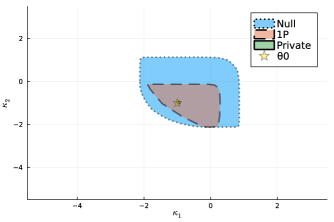
(b) BCE

Figure 1-(a) shows the BSE identified sets obtained under different baseline information structures. The identified sets shrink as the informational assumptions get stronger. We omit the complete information case since $\Theta_{I}^{BSE}\left(S^{private}\right)=\Theta_{I}^{BSE}\left(S^{complete}\right)$. Setting the baseline information structure as $S^{null}$ generates an identified set that is quite permissive while using $S^{private}$ generates a tight identified set. Note that $\Theta_{I}^{BSE}\left(S^{null}\right)$ amounts to making no assumption on what the players minimally observe, and $\Theta_{I}^{BSE}\left(S^{private}\right)$ is equal to the PSNE identified set. Similarly, Figure 1-(b) plots the BCE identified sets obtained under different baseline information structures. It shows that stronger assumptions on information lead to tighter identified sets. Assumptions on players’ information play a crucial role in determining the size of the identified set. In this sense, imposing strong assumption on players’ information may be far from innocuous because it places strong restrictions for identification.

As stated in Theorem 5.3, comparing Figure 1-(a) and 1-(b) shows that, for any given baseline information structure, the corresponding BSE identified set is a subset of the corresponding BCE identified set. In our example, under the same informational assumption, the BSE identified set can be substantially tighter than the BCE identified set, illustrating the identifying power of leveraging observability of opponents’ actions in the equilibrium conditions.

4 Estimation and Inference

We propose a computationally attractive approach for estimation and inference. In Section 4.1, we show that whether a candidate parameter enters the identified set can be determined by solving a single linear feasibility program. In Section 4.2, we show that this property can be combined with the insights from Horowitz and Lee (forthcoming) to make construction of confidence sets simple and computationally tractable: determining whether a candidate parameter enters the confidence set amounts to solving a convex feasibility program. Finally, in Section 4.3, we provide some practical suggestions for computational implementations.

4.1 A Linear Programming Characterization

We provide a computationally attractive characterization of the identified set. Syrgkanis, Tamer, and Ziani (2021) uses a similar characterization, but with Bayes correlated equilibrium. Bayes stable equilibrium and Bayes correlated equilibrium share similar computational property since decision rules enter the equilibrium conditions linearly in both cases.

Let $\Theta_{I}\equiv\Theta_{I}^{BSE}\left(S\right)$ denote the sharp identified set. Let $\partial u_{i}^{x,\theta}\left(a_{i}^{\prime},a,\varepsilon_{i}\right)\equiv u_{i}^{x,\theta}\left(a_{i}^{\prime},a_{-i},\varepsilon_{i}\right)-u_{i}^{x,\theta}\left(a_{i},a_{-i},\varepsilon_{i}\right)$ denote the gains from unilaterally deviating to $a_{i}^{\prime}$ from outcome $\left(a_{i},a_{-i}\right)$ given $\varepsilon_{i}$. Recall our notation that $\sigma^{x}\in\Delta_{a|\varepsilon,t}$ if and only if $\sigma_{a|\varepsilon,t}^{x}\geq 0$ for all $a,\varepsilon,t$ and $\sum_{a\in\mathcal{A}}\sigma_{a|\varepsilon,t}^{x}=1$.

Theorem 6 (Linear programming characterization).

Under Assumptions 1 and 3, $\theta\in\Theta_{I}$ if and only if, for each $x\in\mathcal{X}$, there exists $\sigma^{x}\in\Delta_{a|\varepsilon,t}$ such that

1. (Obedience) For all $i\in\mathcal{I}$, $t_{i}\in\mathcal{T}_{i}$, $a\in\mathcal{A}$, $a_{i}^{\prime}\in\mathcal{A}_{i}$,

   $$\sum_{\varepsilon\in\mathcal{E},t_{-i}\in\mathcal{T}_{-i}}\psi_{\varepsilon}^{x,\theta}\pi_{t|\varepsilon}^{x}\sigma_{a|\varepsilon,t}^{x}\partial u_{i}^{x,\theta}\left(a_{i}^{\prime},a,\varepsilon_{i}\right)\leq 0.$$ (6)

2. (Consistency) For all $a\in\mathcal{A}$,

   $$\phi_{a}^{x}=\sum_{\varepsilon\in\mathcal{E},t\in\mathcal{T}}\psi_{\varepsilon}^{x,\theta}\pi_{t|\varepsilon}^{x}\sigma_{a|\varepsilon,t}^{x}.$$ (7)

Theorem 6 says that for any candidate $\theta\in\Theta$, whether $\theta\in\Theta_{I}$ can be determined by solving a single linear feasibility program. The first condition (6) states that the nuisance parameter $\sigma^{x}$ should be a decision rule that satisfies the Bayes stable equilibrium conditions. The second condition (7) states that the observed conditional choice probabilities must be consistent with those induced by the equilibrium decision rule. Given a candidate $\theta$ as fixed, $\psi_{\varepsilon}^{x,\theta}$, $\pi_{t|\varepsilon}^{x}$, $\partial u_{i}^{x,\theta}$, and $\phi_{a}^{x}$ are known objects. Also note that $\sigma^{x}\in\Delta_{a|\varepsilon,t}$ represent constraints that are linear in $\sigma^{x}$. Then, since the variables of optimization $\sigma^{x}$ enter the constraints linearly, the program is linear.

Since our empirical framework obtains pure strategy Nash equilibrium as a special case, the complete information pure strategy Nash equilibrium identified set can be computed using linear programs as well. Let $\Theta_{I}^{PSNE}$ be the sharp identified set obtained under the pure strategy Nash equilibrium assumption and no assumption on the equilibrium selection rule. As a corollary to Theorem 5 and Theorem 6, whether $\theta\in\Theta_{I}^{PSNE}$ can also be determined via a single linear feasibility program. Thus, Bayes stable equilibrium identified sets embed the pure strategy Nash equilibrium identified set studied in Beresteanu, Molchanov, and Molinari (2011) and Galichon and Henry (2011) as a special case.

Corollary 4 (Linear programming characterization of PSNE identified set).

$\theta\in\Theta_{I}^{PSNE}$ if and only if, for each $x\in\mathcal{X}$, there exists $\sigma^{x}\in\Delta_{a|\varepsilon}$ such that

1. (Obedience) For all $i\in\mathcal{I}$, $\varepsilon_{i}\in\mathcal{E}_{i}$, $a\in\mathcal{A}$, $a_{i}^{\prime}\in\mathcal{A}_{i}$,

   $$\sum_{\varepsilon_{-i}\in\mathcal{E}_{-i}}\psi_{\varepsilon}^{x,\theta}\sigma_{a|\varepsilon}^{x}\partial u_{i}^{x,\theta}\left(a_{i}^{\prime},a,\varepsilon_{i}\right)\leq 0.$$

2. (Consistency) For all $a\in\mathcal{A}$,

   $$\phi_{a}^{x}=\sum_{\varepsilon\in\mathcal{E}}\psi_{\varepsilon}^{x}\sigma_{a|\varepsilon}^{x}.$$

Example (Continued).

Suppose the econometrician wants to identify $\theta=\left(\kappa_{1},\kappa_{2}\right)\in\mathbb{R}^{2}$ based on the population choice probabilities $\phi=\left(\phi_{\left(0,0\right)},\phi_{\left(0,1\right)},\phi_{\left(1,0\right)},\phi_{\left(1,1\right)}\right)\in\mathbb{R}^{4}$. Then $\theta\in\Theta_{I}^{PSNE}$ if and only if there exists $\sigma\in\Delta_{a|\varepsilon}$ such that

$$\sum_{\varepsilon_{-i}}\psi_{\varepsilon}\sigma_{a|\varepsilon}\left(\left(a_{i}^{\prime}-a_{i}\right)\left(\kappa_{i}a_{-i}+\varepsilon_{i}\right)\right)\leq 0,\quad\forall i,\varepsilon_{i},a_{i},a_{-i},a_{i}^{\prime}$$ (8)

$$\phi_{a}=\sum_{\varepsilon}\psi_{\varepsilon}\sigma_{a|\varepsilon},\quad\forall a.$$

which is a linear feasibility program. $\blacksquare$

4.2 A Simple Approach to Inference

We leverage the insights from Horowitz and Lee (forthcoming) and propose a simple approach to inference on the structural parameters. The key idea behind our approach is summarized as follows. In discrete games, all information in the data is summarized by the conditional choice probabilities, as apparent in Theorem 6. The statistical sampling uncertainty arises only from the estimation of the unknown population conditional choice probabilities, which are multinomial proportion parameters. Then, if we control for the sampling uncertainty associated with the estimation of the conditional choice probabilities, we can conduct inference on the structural parameters of interest. This strategy is feasible given that the number of multinomial proportion parameters to estimate is small relative to the sample size. Thus, we construct a confidence set for the conditional choice probabilities, and translate inference on the conditional choice probabilities to inference on the structural parameters using the characterizations in Theorem 6.

Let $\phi\equiv\left(\phi^{x}\right)_{x\in\mathcal{X}}$ be the population choice probabilities. Let us make the dependence of the identified set on $\phi$ explicit by writing

$$\Theta_{I}\equiv\Theta_{I}\left(\phi\right).$$

In other words, the identified set is constructed by inverting the mapping from the structural parameters to the conditional choice probabilities; if we know $\phi$ accurately, then we can obtain the population identified set.

When there is a finite number of observations, $\phi$ is unknown. However, we are able to construct a confidence set for $\phi$ that accounts for the sampling uncertainty. Let $\alpha\in\left(0,1\right)$. We assume that the econometrician can construct a convex confidence set $\Phi_{n}^{\alpha}$ that covers $\phi$ with high probability asymptotically.

Assumption 4 (Convex confidence set for CCP).

Let $\alpha\in\left(0,1\right)$. A set $\Phi_{n}^{\alpha}$ such that

$$\lim\inf_{n\to\infty}\text{Pr}\left(\phi\in\Phi_{n}^{\alpha}\right)\geq 1-\alpha$$

is available. Moreover, $\phi\in\Phi_{n}^{\alpha}$ can be expressed as a collection of convex constraints.

Leading examples of $\Phi_{n}^{\alpha}$ are box constraints or ellipsoid constraints; the former will be characterized by constraints that are linear in $\phi^{x}$ and the latter will be characterized by those quadratic in $\phi^{x}$. For example, we can construct simultaneous confidence intervals for each $\phi_{a}^{x}\in\mathbb{R}$ such that the probability of covering all $\left\{\phi_{a}^{x}\right\}_{a\in\mathcal{A},x\in\mathcal{X}}$ simultaneously is asymptotically no smaller than $1-\alpha$.

Define the confidence set for the identified set as

$$\widehat{\Theta}_{I}^{\alpha}\equiv\bigcup_{\tilde{\phi}\in\Phi_{n}^{\alpha}}\Theta_{I}\left(\tilde{\phi}\right).$$ (9)

By construction, if $\Phi_{n}^{\alpha}$ covers $\phi$ with high probability, then $\widehat{\Theta}_{I}^{\alpha}$ covers $\Theta_{I}$ with high probability.

Theorem 7 (Inference).

Suppose $\Phi_{n}^{\alpha}$ satisfies Assumption 4 and $\widehat{\Theta}_{I}^{\alpha}$ is constructed as (9).

1. $\lim\inf_{n\to\infty}\text{Pr}\left(\Theta_{I}\subseteq\widehat{\Theta}_{I}^{\alpha}\right)\geq 1-\alpha$.

2. For each $\theta$, determining $\theta\in\widehat{\Theta}_{I}^{\alpha}$ solves a convex program.

Theorem 7.1 follows directly from (9) and the assumption on $\Phi_{n}^{\alpha}$. To understand Theorem 7.2, note that $\theta\in\widehat{\Theta}_{I}^{\alpha}$ if and only if, for all $x\in\mathcal{X}$, there exist $\sigma^{x}:\mathcal{E}\times\mathcal{T}\to\Delta\left(\mathcal{A}\right)$ and $\phi^{x}\in\Delta\left(\mathcal{A}\right)$ such that (6), (7), and $\phi\in\Phi_{n}^{\alpha}$ are satisfied. Compared to the population program described in Theorem 6, which treated $\phi$ as known constants, we make $\phi$ part of the optimization variables and impose convex constraints $\phi\in\Phi_{n}^{\alpha}$. Since all equality constraints are linear in $\left(\sigma,\phi\right)$ and inequality constraints are convex in $\left(\sigma,\phi\right)$, the feasibility program is convex (see Boyd and Vandenberghe (2004)). Note that the computational tractability comes from the fact that $\phi$ enters the restrictions in Theorem 6 in an additively separable manner; letting $\phi$ be part of the optimization variable does not disrupt the linearity of the constraints with respect to the variables of optimization.

Finally, we note that computation can be made faster by constructing $\Phi_{n}^{\alpha}$ as linear constraints since then $\theta\in\widehat{\Theta}_{I}^{\alpha}$ can be determined via a linear program. In our empirical application, we construct $\Phi_{n}^{\alpha}$ as simultaneous confidence intervals for the multinomial proportion parameters $\phi$ using the results in Fitzpatrick and Scott (1987).

4.3 Implementation

We propose a practical routine for obtaining the confidence set $\widehat{\Theta}_{I}^{\alpha}$. Theorem 7 says that for any candidate $\theta$, we can determine whether $\theta\in\widehat{\Theta}_{I}^{\alpha}$ by solving a convex (feasibility) program. This feature is attractive, but it only provides us a binary answer (“yes” or “no”).

As commonly done in existing works on partially identified game-theoretic models (e.g., Ciliberto and Tamer (2009), Syrgkanis, Tamer, and Ziani (2021), Magnolfi and Roncoroni (forthcoming)), we define a non-negative criterion function $\widehat{Q}_{n}^{\alpha}\left(\theta\right)\geq 0$ with the property that $\widehat{Q}_{n}^{\alpha}\left(\theta\right)=0$ if and only if $\theta\in\widehat{\Theta}_{I}^{\alpha}$. The value of $\widehat{Q}_{n}^{\alpha}\left(\theta\right)$ for each $\theta$ can be obtained by solving a convex program. The advantage of using a criterion function is that the value of $\widehat{Q}_{n}^{\alpha}\left(\theta\right)$ gives us information on the distance between $\theta$ and the identified set. Moreover, the gradients of the criterion functions provide information on which directions to descend in order to spot a local minimum.

Let $\left\{w^{x}\right\}_{x\in\mathcal{X}}$ be the set of strictly positive weights for each bin $x\in\mathcal{X}$. The choice of weights can be arbitrary although we will choose values proportional to the number of observations at each bin $x$. Let $q^{x}\in\mathbb{R}$ and $q\equiv\left(q^{x}\right)_{x\in\mathcal{X}}$. Let $\widehat{Q}_{n}^{\alpha}\left(\theta\right)$ be the value of the following convex program.

$$\min_{q,\sigma,\phi}\sum_{x\in\mathcal{X}}w^{x}q^{x}\quad\text{subject to }$$ (10)

$$\sum_{\varepsilon,t_{-i}}\psi_{\varepsilon}^{x,\theta}\pi_{t|\varepsilon}^{x}\sigma_{a|\varepsilon,t}^{x}\partial u_{i}^{x,\theta}\left(\tilde{a}_{i},a,\varepsilon_{i}\right)\leq q^{x},\quad\forall i,x,t_{i},a,\tilde{a}_{i}$$

$$\phi_{a}^{x}=\sum_{\varepsilon,t}\psi_{\varepsilon}^{x,\theta}\pi_{t|\varepsilon}^{x}\sigma_{a|\varepsilon,t}^{x},\quad\forall a,x$$

$$q^{x}\geq 0,\ \sigma^{x}\in\Delta_{a|\varepsilon,t},\ \phi^{x}\in\Delta_{a},\quad\forall x$$

$$\phi\in\Phi_{n}^{\alpha}.$$

Intuitively, $q^{x}\geq 0$ measures the minimal violation of the inequalities necessary at bin $x$; when all equilibrium conditions can be satisfied, the solver will drive the value of $q^{x}$ to zero. The solution to (10) measures the weighted average of the minimal violations of the equilibrium conditions required to make $\theta$ compatible with data. Also note that the choice of weights do not affect the results if the researcher is only interested in the set of $\theta$’s whose criterion function values are exactly zero.

The following summarizes the properties of the criterion function approach.

Theorem 8 (Implementation).

1. For any $\theta\in\Theta$, program (10) is feasible and convex.

2. $\widehat{Q}_{n}^{\alpha}\left(\theta\right)=0$ if and only if $\theta\in\widehat{\Theta}_{I}^{\alpha}$.

3. If the gradient $\nabla\widehat{Q}_{n}^{\alpha}\left(\theta\right)$ exists at $\theta$, it can be obtained as a byproduct to program (10) via the envelope theorem.

In particular, Theorem 8.3 says that, due to the envelope theorem, we can obtain the gradients for free when we evaluate the criterion function at each point (assuming the analytic derivatives of $\psi^{x,\theta}$ and $u_{i}^{x,\theta}$ are available). In practice, we need to identify the minimizers of $\widehat{Q}_{n}^{\alpha}\left(\theta\right)$ in order to numerically approximate $\widehat{\Theta}_{I}^{\alpha}$. However, doing so by conducting an extensive grid search over the whole parameter space can be computationally costly especially when the dimension of $\theta$ is high. Due to Theorem 8.3, one can use gradient-based optimization algorithms to identify a minimizer of the criterion function. The ability to quickly identify $\arg\min_{\theta}\widehat{Q}_{n}^{\alpha}\left(\theta\right)$ is advantageous since we can quickly test whether the identified set is empty, or restrict the search to points near the minimizer.

For our empirical application, we use a heuristic approach to approximate $\widehat{\Theta}_{I}^{\alpha}$. The idea is to identify a minimizer of the criterion function and run a random walk process starting from the minimizer in order to collect nearby points that have zero criterion function values. This way we avoid the need to evaluate points that are far from the identified set. See Appendix B.3 for details.

5 Empirical Application: Entry Game by McDonald’s and Burger King in the US

We apply our framework to study the entry game by McDonald’s and Burger King in the US using rich datasets. Entry competition in the fast food industry fits our framework well due to two stylized facts. First, the decisions on whether or not to operate outlets are highly persistent, indicating that the firms’ decisions are publicly observed. Tables 1 and 2 report the three-year transition probability of the firms’ decisions and the market outcomes $\left(a_{MD},a_{BK}\right)$ (where $a_{i}=1$ if firm $i$ is present in the market and $a_{i}=0$ otherwise), measured for all urban census tracts (which correspond to our definition of markets) in the contiguous US over 1997-2019. For instance, the probability that McDonald’s has an outlet in operation in a local market three years later conditional on it having an outlet in operation today is 0.95. Together with the assumption that the costs of revising decisions are sufficiently low, the evidence supports the claim that firms’ decisions are best-responses to opponents’ decisions that are readily observed.

Table 1: Three-year Transition Probability of Decisions

McDonald’s				Burger King
$t\backslash t+3$	Out	In		$t\backslash t+3$	Out	In
Out	0.98	0.02		Out	0.99	0.01
In	0.05	0.95		In	0.08	0.92

• Notes: Measured for urban tracts in the contiguous US, 1997-2019.

Table 2: Three-year Transition Probability of Market Outcomes $\left(a_{MD},a_{BK}\right)$

$t$\$t+3$	$\left(0,0\right)$	$\left(0,1\right)$	$\left(1,0\right)$	$\left(1,1\right)$
$\left(0,0\right)$	0.97	0.01	0.02	0.00
$\left(0,1\right)$	0.09	0.87	0.00	0.04
$\left(1,0\right)$	0.06	0.00	0.92	0.02
$\left(1,1\right)$	0.00	0.04	0.08	0.88

• Notes: Measured for urban tracts in the contiguous US, 1997-2019.

Second, information asymmetries and information spillover from observing others’ decisions are common features in the industry. It is well-documented that competitors take extra scrutiny over the locations where McDonald’s opens new outlets in order to take advantage of McDonald’s leading market research technology. Our notion of equilibrium accounts for this phenomenon.

Using the proposed framework, we estimate the entry game under different baseline information structures in order to explore the role of informational assumptions on identification. We also compare our results to those obtained under Bayes correlated equilibrium, which also allows estimation with weak assumptions on players’ information. We then perform a counterfactual policy exercise that studies how the market structures in Mississippi food deserts respond after increasing access to healthy food.

5.1 Data Description

We combine multiple datasets to construct the final dataset for structural estimation of the entry game. In the final dataset, the unit of observation is a market (urban tract). Each observation contains information on the firms’ market entry decisions and the observable characteristics of the firms and the market.

Our primary dataset comes from Data Axle Historical Business Database, which contains a (approximately) complete list of fast-food chain outlets operating in the US between 1997 and 2019 at an annual level. The advantage of this dataset is that it provides the address information of the burger outlets across all regions of the US. The use of this dataset to study strategic entry decisions is new.

Although we use panel data to investigate the persistence of decisions over time, we use cross-section data to estimate the structural model. The idea is to illustrate that the econometrician can use cross-sectional data as a snapshot of the stable outcomes of the markets at some point in time. We use the 2010 cross-section since it was the last year for which decennial census data were available. We describe the main features of our dataset below. Further details on data construction are provided in Appendix C.

Market Definition

Markets are defined as 2010 urban census tracts in the contiguous US. A census tract is classified as urban if its geographic centroid is in an urbanized area defined by the Census. The final data contain 54,944 markets. We code $a_{i}=1$ if firm $i$ had an outlet operating in the market. The unconditional probabilities of market outcomes are $\left(\hat{\phi}_{00},\hat{\phi}_{01},\hat{\phi}_{10},\hat{\phi}_{11}\right)=\left(0.74,0.06,0.15,0.05\right)$ where $\hat{\phi}_{a}$ is the sample frequency of outcome $a=\left(a_{MD},a_{BK}\right)$.

Exclusion Restrictions

We use two firm-specific variables that have been used in existing works: distance to headquarters (Zhu et al. (2009), Zhu and Singh (2009), Yang (2012)) and own outlets in nearby markets (Toivanen and Waterson (2005), Igami and Yang (2016), Yang (2020)). Variable distance to headquarter measures the distance between the center of each market to the firms’ respective headquarters. The associated exclusion restriction is valid if the cost of operating an outlet increases with its distance to own headquarter, but is unrelated to the distance to opponents’ headquarters. Variable own outlets in neighboring markets is constructed by finding all outlets in tracts that are adjacent to a given tract. The underlying assumption is that an outlet’s profit can be affected by an own-brand outlet in a neighboring market, but not by a competing brand’s outlet in a neighboring market; competition with opponents occur only within each market.

Summary Statistics

Summary statistics are provided in Table 3. Continuous variables are discretized to binary variables by using cutoffs around their medians. Clearly, the entry probability of McDonald’s is higher. McDonald’s is more likely to have an outlet present in adjacent markets. The distance to headquarter is higher for Burger King on average because Burger King has its headquarter in Florida while McDonald’s has its headquarter in Chicago.

Table 3: Summary Statistics

	Mean	Std dev	Min	Max	N
Decision variables
MD Entry	0.196	0.397	0.00	1.00	54940
BK Entry	0.106	0.307	0.00	1.00	54940
Firm-specific variables
MD outlets present in nearby markets	0.720	0.449	0.00	1.00	54940
BK outlets present in nearby markets	0.483	0.500	0.00	1.00	54940
Long distance to MD HQ (>1.6K km)	0.285	0.451	0.00	1.00	54940
Long distance to BK HQ (>1.6K km)	0.712	0.453	0.00	1.00	54940
Market environment variables
Many eating/drinking places (>7 stores)	0.465	0.499	0.00	1.00	54940
High income per capita (>25K dollars)	0.502	0.500	0.00	1.00	54940
Low access to healthy food	0.856	0.351	0.00	1.00	54940
Food desert	0.334	0.472	0.00	1.00	54940

• Notes: All variables are binary. Each observation corresponds to urban census tracts.

Market environment variables control for the determinants of profitability that are common across firms. We obtain the following variables to describe market environments. First, we have an indicator for whether a tract has many eating or drinking places; the variable is obtained from the National Neighborhood Data Archive (NaNDA) which provides business activity information at the tract-level. Second, we have an indicator for whether a tract has high income per capita; the variable is from the census. Finally, from the Food Access Research Atlas, we obtain indicators for whether a tract has low access to healthy food and whether a tract is classified as a food desert. A tract is classified as having low access to healthy food if at least 500 or 33 percent of the population lives more than 1/2 mile from the nearest supermarket, supercenter, or large grocery store. A tract is classified as a food desert if it has low income and low access to healthy food, where the criteria for low-income are from the U.S. Department of Treasury’s New Markets Tax Credit program.

The last rows of Table 3 shows that 85% of all urban census tracts are classified as having low access to healthy food and 33% are classified as food deserts. In the counterfactual analysis, we select food deserts in Mississippi and investigate the impact of increasing access to healthy food on the strategic entry decisions of the firms.

5.2 Preliminary Analysis

Before estimating the structural model, we examine the data patterns using simple probit regressions. Each market $m$ contains binary decisions of each firm $a_{im}\in\left\{0,1\right\}$ where $a_{im}=0$ if firm $i$ stays out in market $m$ and $a_{im}=1$ if $i$ stays in. We pool the decisions of the firms in each market (so that the unit of observation is $\left(i,m\right)$) and regress the binary decisions on market characteristics. Table 4 reports the average marginal effects computed from the regression results.

Table 4: Average Marginal Effects from Simple Probit Models

	(1)	(2)	(3)
	In	In	In
Own-brand outlets present in nearby markets	-0.067	-0.076	-0.096
	(0.002)	(0.002)	(0.002)
Long distance to HQ (> 1.6K km)	-0.083	-0.083	-0.010
	(0.003)	(0.003)	(0.003)
Many eating/drinking places (>7)		0.203	0.203
		(0.002)	(0.002)
High income per capita (>25K dollars)		-0.038	-0.037
		(0.002)	(0.002)
Low access to healthy food		0.039	0.041
		(0.004)	(0.004)
McDonald’s			0.109
			(0.002)
State Dummies	Yes	Yes	Yes
N	107,042	107,042	107,042

• Notes: Each observation corresponds to a firm-market pair. Standard errors, which are given in the parentheses, are clustered at the market-level. All variables are binary.

Table 4 conveys three messages. First, the presence of own outlets in neighboring markets and distance to headquarter are negatively correlated with entry decisions. This appears to be consistent with our prior that these variables have a negative impact on potential profits. Second, the number of eating and drinking places strongly affects the burger chains’ entries. This is presumably because districts with high concentration of food services are also places with high traffic of people who eat out. Finally, low access to healthy food is positively correlated with entry decisions. That is, the burger chains are more likely to enter a market when there are fewer healthy substitutes for food.

While Table 4 provides a helpful snapshot for what drives the chains’ entry decisions, the estimates are likely to be biased since they ignore the fact that firms’ decisions affect each other. Such consideration is crucial not only for estimating the parameters of the model but also for studying a policy experiment. In the next section, we estimate the entry game using Bayes stable equilibrium as a solution concept.

5.3 Entry Game Setup

We posit a canonical entry game that extends the running example to incorporate covariates in the payoff functions. Let us recall the notation. We use $i=1,2$ to denote McDonald’s and Burger King respectively. In each market $m$, firm $i$ can choose a binary action $a_{im}\in\left\{0,1\right\}$ where $a_{im}=1$ if $i$ stays in and $a_{im}=0$ if $i$ stays out. The payoff function is specified as

$$u_{i}^{x_{m},\theta}\left(a_{im},a_{jm},\varepsilon_{im}\right)=a_{im}\left(\beta_{i}^{T}x_{im}+\kappa_{i}a_{jm}+\varepsilon_{im}\right).$$

That is, the payoff from operating in the market is $\beta_{i}^{T}x_{im}+\kappa_{i}a_{jm}+\varepsilon_{im}$ where $x_{im}$ represents market covariates, $a_{jm}$ represents whether the opponent is present, and $\varepsilon_{im}$ is firm $i$’s payoff shock that is not observed by the econometrician. Each $\varepsilon_{im}$ can include firm-specific payoff determinants (e.g., customers’ loyalty to brand and managerial ability) and common payoff determinants (e.g., local food preference, local price level, the degree of competition from other restaurants). We model $\left(\varepsilon_{1m},\varepsilon_{2m}\right)\in\mathbb{R}^{2}$ as being normally distributed with zero mean, unit variance, and correlation coefficient $\rho\in[0,1)$. The payoff from staying out is normalized to zero. Our specification of the payoff functions is quite standard in the literature.

We estimate the parameters under the baseline information assumptions specified previously in Example 1: $S^{null}$, $S^{1P}$, and $S^{private}$. To recap, $S^{null}$ is the information structure in which each player observes nothing; in $S^{1P}$, Player 1 observes (only) $\varepsilon_{1}$ whereas Player 2 observes nothing; in $S^{private}$, Player 1 observes $\varepsilon_{1}$ and Player 2 observes $\varepsilon_{2}$.

Under the Bayes stable equilibrium assumption, the baseline information structures should be interpreted as specifying what the players minimally observe. Then estimating the model with $S^{null}$ as the baseline information structure amounts to making no assumption on players’ information. On the other hand, if the baseline information structure is set to $S^{private}$, then the identified set is robust to all cases in which the players observe at least their payoff shocks. Finally, setting the baseline information structure to $S^{1P}$ amounts to assuming that McDonald’s has good information about its payoff shocks whereas Burger King might minimally have no information about its payoff shock. This assumption relaxes the standard assumption on information (namely the information structure is fixed at either $S^{private}$ or $S^{complete}$) and is consistent with the anecdotal evidence that McDonald’s is a leader in the market research technology.

5.4 Estimation Results

In order to keep the model parsimonious and reduce the computational burden, we take some steps before estimation, which are described as follows (see Appendix B for further details). First, we assume that the coefficients for common market-level variables (eating places, income per capita, and low access to healthy food) are identical across the two players. We also assume that the coefficients of the firm-specific variables (distance to headquarter and the presence of own-brand outlets in nearby markets) are non-positive. Second, while the benchmark distribution of the latent variables $\left(\varepsilon_{1m},\varepsilon_{2m}\right)$ is continuous, we use discretized normal distribution for feasible estimation. Third, we discretize each variable to binary bins; since there are 7 variables in the covariates, this gives $2^{7}=128$ discrete covariate bins. Conditional choice probabilities are non-parametrically estimated using the observations within each bin. Fourth, to construct confidence sets for the conditional choice probabilities, we used simultaneous confidence bands based on the method described in Fitzpatrick and Scott (1987); using simultaneous confidence bands makes the evaluation of the criterion function a linear program.

5.4.1 The Role of Informational Assumptions on Identification

Table 5: Bayes Stable Equilibrium Identified Sets

Baseline Information	$S^{null}$	$S^{1P}$	$S^{private}$
McDonald’s Variables
Spillover Effects	$[-1.83,1.62]$	$[-0.89,-0.14]$	-
Constant	$[-1.64,0.32]$	$[-1.46,-1.04]$	-
Nearby Outlets	$[-1.24,-0.00]$	$[-0.56,-0.25]$	-
Distance to HQ	$[-1.23,-0.00]$	$[-0.26,-0.00]$	-
Burger King Variables
Spillover Effects	$[-1.81,1.22]$	$[-1.19,-0.25]$	-
Constant	$[-2.38,0.44]$	$[-1.48,-0.76]$	-
Nearby Outlets	$[-1.44,-0.00]$	$[-0.53,-0.00]$	-
Distance to HQ	$[-1.41,-0.00]$	$[-0.52,-0.00]$	-
Common Market-level Variables
Eating Places	$[-0.31,1.87]$	$[0.82,1.21]$	-
Income Per Capita	$[-1.02,0.75]$	$[-0.54,-0.18]$	-
Low Access	$[-0.71,1.31]$	$[0.25,0.54]$	-
Correlation parameter $\rho$	$[0.00,0.99]$	$[0.42,0.91]$	-
Number of Markets	54940	54940	54940

• Notes: Table reports the projections of confidence sets obtained with nominal level $\alpha=0.05$. The identified set for $S^{private}$ not reported because it is empty.

Table 5 reports projections of the 95% confidence sets obtained under the Bayes stable equilibrium assumption with different baseline information structures. There are three main findings related to the role of informational assumption. First, making no assumption on players’ information leads to an uninformative identified set. The confidence set under $S^{null}$ is quite large, and we cannot determine the signs of the parameters. Therefore, being utterly agnostic about players’ information does not give us enough identifying power to draw meaningful conclusions.

Second, standard assumptions on information may be too strong. It is quite standard to assume that each player $i$ observes (exactly) $\varepsilon_{i}$ or $\left(\varepsilon_{i},\varepsilon_{-i}\right)$. Setting baseline information structure as $S^{private}$ nests all these cases. However, we find that the identified set under $S^{private}$ is empty, suggesting the possibility of misspecification. Thus, assuming that each player observes at least their $\varepsilon_{i}$ may be too strong. Since the Bayes stable equilibrium identified set under $S^{private}$ is equivalent to the pure strategy Nash equilibrium identified set (see Theorem 5.2), the pure strategy Nash equilibrium assumption would also be rejected.

Third, we find that setting the baseline information structure to $S^{1P}$ can produce an informative identified set. Recall that the identified set under $S^{1P}$ makes the assumption that McDonald’s has accurate information about its payoff shock, but Burger King’s information can be arbitrary. This assumption is consistent with the anecdotal evidence that McDonald’s has superior information on the potential profitability of each market, and Burger King tries to free-ride on McDonald’s information by observing what McDonald’s does. Table 5 shows that, even if we substantially relax the assumption on Burger King’s information, we can determine the signs of the most parameters. For example, we can see that burger chains are more likely to enter in markets that have low access to healthy food. We can also learn that the firms’ payoff shocks are highly correlated to each other.

In conclusion, we find that the informativeness of the identified set crucially depends on the underlying assumption on players’ information. At least in our empirical application, it is difficult to draw a meaningful economic conclusion without making assumptions on players’ information. On the other hand, under the maintained solution concept, the model rejects the popular assumptions made in the literature, namely that each firm $i$ observes at least its $\varepsilon_{i}$. A credible intermediate case $S^{1P}$, which is consistent with our knowledge of the market research technology in the fast food industry, delivers strong identifying power.

5.4.2 Comparison to Bayes Correlated Equilibrium Identified Sets

Table 6: Bayes Correlated Equilibrium Identified Sets

Baseline Information	$S^{null}$	$S^{1P}$	$S^{private}$
McDonald’s Variables
Spillover Effects	$[-4.83,1.92]$	$[-4.85,-0.17]$	$[-4.85,-2.11]$
Constant	$[-1.64,0.34]$	$[-1.53,0.29]$	$[-1.37,0.31]$
Nearby Outlets	$[-1.33,-0.00]$	$[-1.11,-0.00]$	$[-0.97,-0.00]$
Distance to HQ	$[-1.35,-0.00]$	$[-1.10,-0.00]$	$[-0.88,-0.00]$
Burger King Variables
Spillover Effects	$[-3.84,3.33]$	$[-3.98,0.72]$	$[-3.38,-1.03]$
Constant	$[-3.71,0.61]$	$[-1.65,0.62]$	$[-1.62,0.44]$
Nearby Outlets	$[-1.71,-0.00]$	$[-1.23,-0.00]$	$[-1.11,-0.00]$
Distance to HQ	$[-1.70,-0.00]$	$[-1.03,-0.00]$	$[-0.86,-0.00]$
Common Market-level Variables
Eating Places	$[-0.24,1.98]$	$[0.51,1.76]$	$[0.49,1.68]$
Income Per Capita	$[-1.32,0.84]$	$[-1.16,0.14]$	$[-1.08,0.11]$
Low Access	$[-0.59,1.49]$	$[-0.37,1.31]$	$[-0.28,1.07]$
Correlation parameter $\rho$	$[0.00,0.99]$	$[0.00,0.99]$	$[0.00,0.97]$
BSE volume/BCE volume	0.05036	0.00000	-
Number of Markets	54940	54940	54940

• Notes: Table reports the projections of confidence sets obtained with nominal level $\alpha=0.05$. BSE/BCE volume computed by taking products of projected intervals.

We compare the Bayes stable equilibrium identified sets to the Bayes correlated equilibrium identified sets studied in Magnolfi and Roncoroni (forthcoming). The Bayes correlated equilibrium identified sets are reported in Table 6. We can readily see that the Bayes correlated equilibrium assumption produces a much larger set for each baseline information structure. Even when we set $S^{private}$ as the baseline information structure, it is not easy to learn the signs of many parameters. For example, we cannot determine whether low access to healthy food promotes or deters entries by the burger chains.

Comparing Tables 5 and 6 suggests that if the researcher is willing to accept the Bayes stable equilibrium assumption, it can add significant identifying power while providing the same kind of informational robustness as Bayes correlated equilibria. At least in the context of our empirical application, we believe it is reasonable to assume that McDonald’s decisions that we observe in the data represent best-responses to the observed decisions of Burger King and vice versa.

5.5 Counterfactual Analysis: The Impact of Increasing Access to Healthy Food on Market Structure

Consumption of fast food is driven not only by consumers’ taste for fast food but also the availability of food substitutes in the neighborhood. Following the recent surge of interest on the relationship between food deserts and food consumption patterns (see, e.g., Allcott et al. (2019) and Kolb (2021)), we study the impact of accessibility to healthy food on the entry decisions of fast-food chains. Specifically, we consider a policy experiment to predict changes in market structure in Mississippi food deserts after increasing access to healthy food measured by supermarket entries. Mississippi is often called one of the “hungriest” states in the US. Mississippi had 664 census tracts in 2010, and 329 of them are classified as urban tracts, which correspond to our definition of markets. Out of 329 urban tracts, 185 tracts (approximately 56%) are classified as food deserts, according to the U.S. Department of Agriculture. According to the definition of food deserts, all of these tracts are classified as having low access to healthy food.

We conduct a policy experiment as follows. We select the 185 tracts classified as food deserts in Mississippi and then increase access to healthy food. This amounts to changing the low access indicator from one (low access) to zero (high access) in all these markets. In reality, such policy would correspond to increasing healthy food providers (large grocery stores, supermarkets, or supercenters) by providing subsidies or tax breaks. We then recompute the equilibria in these markets and report the weighted average of the bounds associated with each measure of market structure. See Appendix B.4 for computational details.

We report the results of the counterfactual analysis in Table 7. The first column reports the estimates obtained from the data of the 185 markets corresponding to Mississippi food deserts. For example, the probability of observing McDonald’s enter the market in Mississippi food deserts is 0.30, much larger than the unconditional probability obtained using all markets, which was around 0.20.

Table 7: The Impact of Increasing Access to Healthy Food in Mississippi Food Deserts

			$BSE(S^{1P})$			$BCE(S^{1P})$
	Data		Pre	Post		Pre	Post
Expected number of entrants	$0.47$		$[0.28,1.01]$	$[0.15,0.79]$		$[0.10,1.18]$	$[0.03,1.17]$
Probability of MD entry	$0.30$		$[0.11,0.32]$	$[0.04,0.23]$		$[0.00,0.71]$	$[0.00,0.67]$
Probability of BK entry	$0.17$		$[0.00,0.84]$	$[0.00,0.72]$		$[0.00,1.00]$	$[0.00,1.00]$
Probability of no entrant	$0.64$		$[0.15,0.74]$	$[0.28,0.85]$		$[0.00,0.90]$	$[0.00,0.97]$

• Notes: Data column represents the sample estimates obtained using markets corresponding to Mississippi food deserts. Final bounds obtained by simulating equilibria at each parameter in the identified set, and then taken union over all bounds. Each number is obtained by taking a weighted average with weights proportional to the number of markets in each covariate bin.

The second and third columns report the bounds obtained before (“Pre” has low access indicators set to one) and after the counterfactual policy (“Post” has low access indicators set to zero) using the $S^{1P}$-Bayes stable equilibrium identified set. The bounds are pretty wide because we have considered all parameters in the identified set and made no assumption on the equilibrium selection. However, they shift in the expected directions. For example, the bounds on the expected number of entrants shift from $[0.28,1.01]$ to $[0.15,0.79]$. Since the mean number of entrants in the data was $0.47$ and the post-counterfactual bounds are $\left[0.15,0.79\right]$, the maximal change we can expect is $0.15-0.47=-0.32$. In some cases, we can make a stronger statement: while the unconditional probability of observing McDonald’s enter in data was 0.30, the upper bound in the Post-regime decreases to 0.23, so we can expect that the probability of McDonald’s enter to decrease by at least 0.07.

Our results suggest that meaningful counterfactual statements may be made even with weak assumptions on players’ information. The bounds do not depend on specific assumptions on equilibrium selection and admit all information structures that are expansions of the baseline information structure. Hence our approach can also serve as a useful tool to conduct sensitivity analysis for researchers who want to see whether their predictions are driven by assumptions on equilibrium selection or what the players know.

For comparison, in the last two columns, we report the counterfactual results obtained using the $S^{1P}$-Bayes correlated equilibrium identified set. One can readily see that the bounds are quite large compared to the Bayes stable equilibrium counterpart. For example, we cannot make any statement about the probability of Burger King’s entry after the counterfactual policy is implemented. Table 7 shows that Bayes correlated equilibrium predictions can be too permissive, especially when no assumption is imposed on what equilibrium might be selected in the counterfactual world.

6 Conclusion

This paper presents an empirical framework for analyzing stable outcomes with weak assumptions on players’ information. We propose Bayes stable equilibrium as a framework for analyzing stable outcomes, which appear in various empirical settings. Our framework can be an attractive alternative to existing methods for practitioners who want to work with an empirical game-theoretic model and be robust to informational assumptions. Furthermore, we believe the proposed computational algorithms can also be helpful in similar settings, especially since reducing computational burden remains a fundamental challenge in the literature.

We believe there are many exciting avenues for future research. First, providing a non-cooperative foundation to our solution concepts remains an open question. While we can imagine a dynamic adjustment process that converges to stable outcomes, how to formalize this idea is yet unclear. Second, it will be interesting to find reasonable ways of imposing equilibrium selection. While Bayes stable equilibrium (or Bayes correlated equilibrium) has the informational robustness property, the set of predictions may be too large, limiting our ability to make sharp predictions for counterfactual analysis. Finding ways to sharpen predictions without sacrificing robustness to information will be helpful. Third, our counterfactual analysis is limited to a partial equilibrium analysis. It will be interesting to think about ways to model the strategic interactions of healthy food providers and unhealthy food providers together. Finally, there are other forms of informational robustness that our model cannot handle but is empirically interesting. For example, it might be natural to assume that McDonald’s has superior information relative to Burger King while being agnostic about their specific information structure. Our model only specifies what the players minimally observe and is agnostic about the relative information across players. Studying alternative forms of informational robustness and corresponding econometric frameworks should be interesting.

Appendix

Appendix A Proofs

A.1 Proof of Theorem 1

Let $S^{*}$ be an expansion of $S$. Let $\delta:\mathcal{T}\times\tilde{\mathcal{T}}\to\Delta\left(\mathcal{A}\right)$ be an outcome function in $\left(G,S^{*}\right)$. We say that an outcome function $\delta$ in $\left(G,S^{*}\right)$ induces a decision rule $\sigma:\mathcal{E}\times\mathcal{T}\to\Delta\left(\mathcal{A}\right)$ in $\left(G,S\right)$ if

$$\sigma\left(a|\varepsilon,t\right)=\sum_{\tilde{t}}\lambda\left(\tilde{t}|\varepsilon,t\right)\delta\left(a|t,\tilde{t}\right)$$

for each $a$ whenever $\text{Pr}\left(\varepsilon,t\right)>0$.

Lemma 1.

A decision rule $\sigma$ is a Bayes stable equilibrium of $\left(G,S\right)$ if and only if, for some expansion $S^{*}$ of $S$, there is a rational expectations equilibrium of $\left(G,S^{*}\right)$ that induces $\sigma$.

The proof of Lemma 1 closely follows the proof in Theorem 1 of Bergemann and Morris (2016). The only if $\left(\Rightarrow\right)$ direction is established by (i) letting the Bayes stable equilibrium decision rule $\sigma$ a signal function that generates public signals (recommendations of outcomes) for every given $\left(\varepsilon,t\right)$, and (ii) constructing an outcome function $\delta$ as a degenerate self-map that places unit mass on $a$ whenever $a$ is drawn from $\sigma\left(\cdot|\varepsilon,t\right)$. Conversely, the if $\left(\Leftarrow\right)$ direction is established by constructing a decision rule by integrating out the players’ signals from a given outcome function.

Proof of Lemma 1.

$\left(\Rightarrow\right)$ Suppose $\sigma$ is a Bayes stable equilibrium of $\left(G,S\right)$. That is,

$$\sum_{\varepsilon,t_{-i}}\psi_{\varepsilon}\pi_{t|\varepsilon}\sigma_{a|\varepsilon,t}u_{i}\left(a,\varepsilon\right)\geq\sum_{\varepsilon,t_{-i}}\psi_{\varepsilon}\pi_{t|\varepsilon}\sigma_{a|\varepsilon,t}u_{i}\left(a_{i}^{\prime},a_{-i},\varepsilon\right),\quad\forall i,t_{i},a,a_{i}^{\prime}.$$

We want to find an expansion $S^{*}$ of $S$ and a rational expectations equilibrium outcome function $\delta$ in $\left(G,S^{*}\right)$ that induces $\sigma$. Construct an expansion $S^{*}$ of $S$ as follows. With some abuse in notation, let $\lambda$ be a signal distribution that generates a public signal such that

$$\lambda\left(\tilde{t}^{p}=a|\varepsilon,t\right)=\sigma\left(a|\varepsilon,t\right).$$

where $\tilde{t}^{p}$ denotes a public signal. Let an outcome function be degenerate as follows:

$$\delta\left(\tilde{a}|t,\tilde{t}^{p}=a\right)=\begin{cases}1&\text{if }\tilde{a}=a\\ 0&\text{if }\tilde{a}\neq a\end{cases}.$$

That is, when the players observe $\tilde{t}^{p}=a$ as a public signal, the outcome function dictates that $a$ be played as an outcome of the game. It remains to show that every outcome $a$ generated by the outcome function $\delta$ is optimal to the players. The rational expectations equilibrium condition is

$$\sum_{\varepsilon,t_{-i}}\psi_{\varepsilon}\pi_{t|\varepsilon}\lambda_{\tilde{t}^{p}|\varepsilon,t}\delta_{\tilde{a}|t,\tilde{t}^{p}}u_{i}\left(\tilde{a},\varepsilon\right)\geq\sum_{\varepsilon,t_{-i}}\psi_{\varepsilon}\pi_{t|\varepsilon}\lambda_{\tilde{t}^{p}|\varepsilon,t}\delta_{\tilde{a}|t,\tilde{t}^{p}}u_{i}\left(\tilde{a}_{i}^{\prime},\tilde{a}_{-i},\varepsilon\right),\quad\forall i,t_{i},\tilde{t}^{p},\tilde{a},\tilde{a}_{i}^{\prime}$$

But since $\lambda\left(\tilde{t}^{p}=a|\varepsilon,t\right)=\sigma\left(a|\varepsilon,t\right)$ and the inequality is trivially satisfied when $\tilde{t}^{p}\neq\tilde{a}$ (both sides become zero), the rational expectations equilibrium condition reduces to

$$\sum_{\varepsilon,t_{-i}}\psi_{\varepsilon}\pi_{t|\varepsilon}\sigma_{a|\varepsilon,t}u_{i}\left(a,\varepsilon\right)\geq\sum_{\varepsilon,t_{-i}}\psi_{\varepsilon}\pi_{t|\varepsilon}\sigma_{a|\varepsilon,t}u_{i}\left(\tilde{a}_{i}^{\prime},a_{-i},\varepsilon\right),\quad\forall i,t_{i},a,\tilde{a}_{i}^{\prime}$$

which holds by the assumption that $\sigma$ is a Bayes stable equilibrium of $\left(G,S\right)$.

$\left(\Leftarrow\right)$ Suppose that $\delta$ is a rational expectations equilibrium of $\left(G,S^{*}\right)$ and $\delta$ induces $\sigma$ in $\left(G,S\right)$. That is, we have

$$\sum_{\varepsilon,t_{-i},\tilde{t}_{-i}}\psi_{\varepsilon}\pi_{t|\varepsilon}\lambda_{\tilde{t}|\varepsilon,t}\delta_{a|t,\tilde{t}}u_{i}\left(a,\varepsilon\right)\geq\sum_{\varepsilon,t_{-i},\tilde{t}_{-i}}\psi_{\varepsilon}\pi_{t|\varepsilon}\lambda_{\tilde{t}|\varepsilon,t}\delta_{a|t,\tilde{t}}u_{i}\left(a_{i}^{\prime},a_{-i},\varepsilon\right),\quad\forall i,t_{i},\tilde{t}_{i},a,a_{i}^{\prime}$$

Integrating out $\tilde{t}_{i}$ from both sides gives

$$\sum_{\varepsilon,t_{-i}}\psi_{\varepsilon}\pi_{t|\varepsilon}\left(\sum_{\tilde{t}}\lambda_{\tilde{t}|\varepsilon,t}\delta_{a|t,\tilde{t}}\right)u_{i}\left(a,\varepsilon\right)\geq\sum_{\varepsilon,t_{-i}}\psi_{\varepsilon}\pi_{t|\varepsilon}\left(\sum_{\tilde{t}}\lambda_{\tilde{t}|\varepsilon,t}\delta_{a|t,\tilde{t}}\right)u_{i}\left(a_{i}^{\prime},a_{-i},\varepsilon\right),\quad\forall i,t_{i},a,a_{i}^{\prime}$$

$$\Leftrightarrow\sum_{\varepsilon,t_{-i}}\psi_{\varepsilon}\pi_{t|\varepsilon}\sigma_{a|\varepsilon,t}u_{i}\left(a,\varepsilon\right)\geq\sum_{\varepsilon,t_{-i}}\psi_{\varepsilon}\pi_{t|\varepsilon}\sigma_{a|\varepsilon,t}u_{i}\left(a_{i}^{\prime},a_{-i},\varepsilon\right),\quad\forall i,t_{i},a,a_{i}^{\prime}$$

which is the Bayes stable equilibrium condition for $\sigma$ in $\left(G,S\right)$. ∎

The statement of the theorem then follows directly from Lemma 1 because any decision rule $\sigma:\mathcal{E}\times\mathcal{T}\to\Delta\left(\mathcal{A}\right)$ in $\left(G,S\right)$ pins down the joint distribution on $\mathcal{E}\times\mathcal{T}\times\mathcal{A}$ (the prior distribution $\psi$ on $\mathcal{E}$ is fixed by $G$ and the signal distribution $\pi:\mathcal{E}\to\Delta\left(\mathcal{T}\right)$ is fixed by $S$). $\square$

A.2 Proof of Corollary 1

$\left(\subseteq\right)$ Take any $\phi\in\text{$\mathcal{P}_{a}^{BSE}\left(G,S\right)$}$. By definition, there is a BSE $\sigma$ in $\left(G,S\right)$ that induces $\phi$. By Theorem 1, there exists an expansion $S^{*}$ of $S$ and a REE $\delta$ of $\left(G,S^{*}\right)$ that induces $\sigma$. Since $\delta$ induces $\sigma$ and $\sigma$ induces $\phi$, $\delta$ induces $\phi$. It follows that $\phi\in\bigcup_{S^{*}\succsim_{E}S}\mathcal{P}_{a}^{REE}\left(G,S^{*}\right)$.

$\left(\supseteq\right)$ Take any $\phi\in\bigcup_{S^{*}\succsim_{E}S}\mathcal{P}_{a}^{REE}\left(G,S^{*}\right)$. By definition, there exists some $S^{*}\succsim_{E}S$ and a REE $\delta$ of $\left(G,S^{*}\right)$ such that $\delta$ induces $\phi$, (i.e., $\phi_{a}=\sum_{\varepsilon,t,\tilde{t}}\psi_{\varepsilon}\pi_{t|\varepsilon}\lambda_{\tilde{t}|\varepsilon,t}\delta_{a|t,\tilde{t}}$ for all $a\in\mathcal{A}$). Since $S^{*}\succsim_{E}S$ and $\delta$ is a REE of $\left(G,S^{*}\right)$, by Theorem 1, $\delta$ induces a decision rule $\sigma$ in $\left(G,S\right)$ that is a BSE of $\left(G,S\right)$. Since $\delta$ induces $\sigma$, it follows that $\sigma$ induces $\phi$. Therefore, we have $\phi\in\text{$\mathcal{P}_{a}^{BSE}\left(G,S\right)$}$. $\square$

A.3 Proof of Corollary 2

Take $\sigma\in\mathcal{P}_{t,\varepsilon,a}^{BSE}\left(G,S\right)$. We want to show that $\sigma\in\mathcal{P}_{\varepsilon,t,a}^{BSE}\left(G,S^{\prime}\right)$. From Theorem 1, we have $\mathcal{P}_{\varepsilon,t,a}^{BSE}\left(G,S\right)=\bigcup_{\tilde{S}\succsim_{E}S}\mathcal{P}_{\varepsilon,t,a}^{REE}\left(G,\tilde{S}\right)$, so there exists some $S^{*}$ such that $\sigma\in\mathcal{P}_{\varepsilon,t,a}^{REE}\left(G,S^{*}\right)$. But since $S^{*}\succsim_{E}S\succsim_{E}S^{\prime}$, we have $\mathcal{P}_{\varepsilon,t,a}^{REE}\left(G,S^{*}\right)\subseteq\bigcup_{\tilde{S}\succsim_{E}S^{\prime}}\mathcal{P}_{\varepsilon,t,a}^{REE}\left(G,\tilde{S}\right)$, so it follows that

$$\sigma\in\bigcup_{\tilde{S}\succsim_{E}S^{\prime}}\mathcal{P}_{\varepsilon,t,a}^{REE}\left(G,\tilde{S}\right)=\mathcal{P}_{\varepsilon,t,a}^{BSE}\left(G,S^{\prime}\right)$$

which is what we wanted. $\square$

A.4 Proof of Theorem 2

1. We first prove the first statement:
   $\left(\Rightarrow\right)$ Since $\delta$ is a REE of $\left(G,S^{complete}\right)$, it satisfies

   $$\psi_{\varepsilon}\delta_{a|\varepsilon}u_{i}\left(a,\varepsilon\right)\geq\psi_{\varepsilon}\delta_{a|\varepsilon}u_{i}\left(a_{i}^{\prime},a_{-i},\varepsilon\right),\quad\forall i,\varepsilon,a,a_{i}^{\prime}.$$

   Fix any $\varepsilon^{*}\in\mathcal{E}$ such that $\psi_{\varepsilon^{*}}>0$ (with the full support assumption, we have $\psi_{\varepsilon}>0$ for all $\varepsilon$). Consider any $a^{*}\in\mathcal{A}$ such that $\delta$ places a positive mass at $\varepsilon^{*}$, i.e., $\delta_{a^{*}|\varepsilon^{*}}>0$. Since $\psi_{\varepsilon^{*}}\delta_{a^{*}|\varepsilon^{*}}>0$, the REE condition reduces to

   $$u_{i}\left(a^{*},\varepsilon^{*}\right)\geq u_{i}\left(a_{i}^{\prime},a_{-i}^{*},\varepsilon^{*}\right),\quad\forall i,a_{i}^{\prime}$$

   which is exactly the PSNE condition of $a^{*}$ at state $\varepsilon^{*}$.

   $\left(\Leftarrow\right)$ Suppose that $\delta:\mathcal{E}\to\Delta\left(\mathcal{A}\right)$ is constructed in a way such that $\delta_{a|\varepsilon}>0$ implies that $a$ is a PSNE outcome at $\varepsilon$. Since any on-path outcome $a$ at $\varepsilon$ is a PSNE at $\varepsilon$, it immediately follows that the outcome is optimal to each player who observes $\left(a_{i},a_{-i}\right)$ and $\varepsilon$, satisfying the REE condition.
   The second statement follows by observing that an outcome function and a decision rule are equivalent (i.e., $\delta\left(a|\varepsilon\right)\equiv\sigma\left(a|\varepsilon,t=\varepsilon\right)$) when the signal distribution is degenerate ($\pi\left(t=\varepsilon|\varepsilon\right)=1$). In this case, the Bayes stable equilibrium conditions reduces to the rational expectations equilibrium conditions. $\square$

2. The first statement is proven as follows:
   ($\Leftarrow$) Let $\delta:\mathcal{E}\to\Delta\left(\mathcal{A}\right)$ be a REE of $\left(G,S^{complete}\right)$. By definition, we have

   $$\psi_{\varepsilon}\delta_{a|\varepsilon}u_{i}\left(a,\varepsilon_{i}\right)\geq\psi_{\varepsilon}\delta_{a|\varepsilon}u_{i}\left(a_{i}^{\prime},a_{-i},\varepsilon_{i}\right),\quad\forall i,\varepsilon,a,a_{i}^{\prime}$$

   Integrating both sides with respect to $\varepsilon_{-i}$ gives

   $$\sum_{\varepsilon_{-i}}\psi_{\varepsilon}\delta_{a|\varepsilon}u_{i}\left(a,\varepsilon_{i}\right)\geq\sum_{\varepsilon_{-i}}\psi_{\varepsilon}\delta_{a|\varepsilon}u_{i}\left(a_{i}^{\prime},a_{-i},\varepsilon_{i}\right),\quad\forall i,\varepsilon_{i},a,a_{i}^{\prime}$$

   which is exactly the REE condition for $\left(G,S^{private}\right)$.

   $\left(\Rightarrow\right)$ Conversely, let $\delta:\mathcal{E}\to\Delta\left(\mathcal{A}\right)$ be a REE of $\left(G,S^{private}\right)$. To show that $\delta$ is a REE of $\left(G,S^{complete}\right)$, by Theorem 2.1, it is enough to show that for each $\varepsilon$, $\delta_{a|\varepsilon}>0$ implies that $a$ is a PSNE of $\Gamma_{\varepsilon}$.
   Since $\delta$ is a REE of $\left(G,S^{private}\right)$, by definition, we have

   $$\sum_{\varepsilon_{-i}}\psi_{\varepsilon}\delta_{a|\varepsilon}u_{i}\left(a,\varepsilon_{i}\right)\geq\sum_{\varepsilon_{-i}}\psi_{\varepsilon}\delta_{a|\varepsilon}u_{i}\left(a_{i}^{\prime},a_{-i},\varepsilon_{i}\right),\quad\forall i,\varepsilon_{i},a,a_{i}^{\prime}$$

   $$\Leftrightarrow\varphi\left(a,\varepsilon_{i}\right)u_{i}\left(a,\varepsilon_{i}\right)\geq\varphi\left(a,\varepsilon_{i}\right)u_{i}\left(a_{i}^{\prime},a_{-i},\varepsilon_{i}\right),\quad\forall i,\varepsilon_{i},a,a_{i}^{\prime}$$

   where $\varphi\left(a,\varepsilon_{i}\right):=\sum_{\varepsilon_{-i}}\psi_{\varepsilon}\delta_{a|\varepsilon}$.
   Now fix $\varepsilon$ and consider any $a$ such that $\delta_{a|\varepsilon}>0$. But $\delta_{a|\varepsilon}>0$ implies $\varphi\left(a,\varepsilon_{i}\right)>0$ which in turn implies that

   $$u_{i}\left(a,\varepsilon_{i}\right)\geq u_{i}\left(a_{i}^{\prime},a_{-i},\varepsilon_{i}\right),\quad\forall i,a_{i}^{\prime}$$

   which is exactly the PSNE condition of $a$ at $\varepsilon$.
   The second statement follows similarly as above; under $S^{private}$, outcome functions and decision rules are equivalent since players’ signals exhaust information about the state of the world.$\square$

A.5 Proof of Theorem 4

Let $S\equiv\left(S^{x}\right)_{x\in\mathcal{X}}$ and $\tilde{S}\equiv\left(\tilde{S}^{x}\right)_{x\in\mathcal{X}}$. Let $\tilde{S}\succsim_{E}S$ if and only if $\tilde{S}^{x}\succsim_{E}S^{x}$ for each $x\in\mathcal{X}$. We want to show

$$\Theta_{I}^{BSE}\left(S\right)=\bigcup_{\tilde{S}\succsim_{E}S}\Theta_{I}^{REE}\left(\tilde{S}\right).$$

Note that

$$\Theta_{I}^{BSE}\left(S\right)\equiv\left\{\theta\in\Theta:\ \forall x\in\mathcal{X},\ \phi^{x}\in\mathcal{P}_{a}^{BSE}\left(G^{x,\theta},S^{x}\right)\right\}$$ (11)

and

$$\bigcup_{\tilde{S}\succsim_{E}S}\Theta_{I}^{REE}\left(\tilde{S}\right) \equiv\bigcup_{\tilde{S}\succsim_{E}S}\left\{\theta\in\Theta:\ \forall x\in\mathcal{X},\ \phi^{x}\in\mathcal{P}_{a}^{REE}\left(G^{x,\theta},\tilde{S}^{x}\right)\right\}$$

$$=\left\{\theta\in\Theta:\ \forall x\in\mathcal{X},\ \phi^{x}\in\bigcup_{\tilde{S}^{x}\succsim_{E}S^{x}}\mathcal{P}_{a}^{REE}\left(G^{x,\theta},\tilde{S}^{x}\right)\right\}.$$ (12)

By Corollary 1, for any given $\theta\in\Theta$ and $x\in\mathcal{X}$, we have

$$\mathcal{P}_{a}^{BSE}\left(G^{x,\theta},S^{x}\right)=\bigcup_{\tilde{S}^{x}\succsim_{E}S^{x}}\mathcal{P}_{a}^{REE}\left(G^{x,\theta},\tilde{S}^{x}\right).$$ (13)

That (11) and (12) are equal follows from (13), which is what we wanted. $\square$

A.6 Proof of Theorem 5

1. Let $G$ be an arbitrary basic game. We suppress the covariates $x$ since they do not play a role. Let $S^{1}$ and $S^{2}$ be arbitrary information structures such that $S^{1}\succsim_{E}S^{2}$. It is enough to show that a BSE in $\left(G,S^{1}\right)$ always induces a BSE in $\left(G,S^{2}\right)$ because it will imply that the set of feasible CCPs in $\left(G,S^{1}\right)$ is a subset of the feasible CCPs in $\left(G,S^{2}\right)$. But this directly follows from Corollary 2. $\square$

2. The statement follows from Theorem 2. In particular, note that when pure strategy Nash equilibrium is the relevant solution concept, the decision rule (or the outcome function) simply represents an arbitrary equilibrium selection mechanism; no assumption is placed on the equilibrium selection rule. Since the set of probability distributions over $\mathcal{A}$ on each realization of $\varepsilon$ is the same across Bayes stable equilibria and pure strategy Nash equilibria, the resulting identified set of parameters must be identical. $\square$

3. The statement follows from Theorem 3. Theorem 3 says that for any $\left(G,S\right)$, if a decision rule $\sigma$ in $\left(G,S\right)$ is a Bayes stable equilibrium of $\left(G,S\right)$, then it is a Bayes correlated equilibrium of $\left(G,S\right)$. This implies that we will have $\mathcal{P}_{a}^{BSE}\left(G,S\right)\subseteq\mathcal{P}_{a}^{BCE}\left(G,S\right)$ for any $\left(G,S\right)$, which leads to the statement. $\square$

A.7 Proof of Theorem 7

1. The first statement follows directly from construction:

   $$\text{Pr}\left(\Theta_{I}\subseteq\widehat{\Theta}_{I}^{\alpha}\right) =\text{Pr}\left(\Theta_{I}\left(\phi\right)\subseteq\bigcup_{\tilde{\phi}\in\Phi_{n}^{\alpha}}\Theta_{I}\left(\tilde{\phi}\right)\right)\geq\text{Pr}\left(\phi\in\Phi_{n}^{\alpha}\right)$$

   (The inequality follows from the possibility that there may exist $\bar{\phi}\neq\phi$ such that $\bar{\phi}\in\Phi_{n}^{\alpha}$ but $\Theta_{I}\left(\phi\right)\subseteq\Theta_{I}\left(\bar{\phi}\right)$.) Taking the limits on both sides gives the desired result. $\square$

2. The second statement follows from the fact that $\phi$ enters the population program (see Theorem 6) in an additively separable manner, and that $\phi\in\Phi_{n}^{\alpha}$ represents a set of convex constraints. To see this, note that $\theta\in\widehat{\Theta}_{I}^{\alpha}$ if and only if the following program is feasible: For each $x\in\mathcal{X}$, find $\sigma^{x}\in\Delta_{a|\varepsilon,t}$ and $\phi^{x}\in\Delta_{a}$ such that

   $$\sum_{\varepsilon,t_{-i}}\psi_{\varepsilon}^{x,\theta}\pi_{t|\varepsilon}^{x}\sigma_{a|\varepsilon,t}^{x}\partial u_{i}^{x,\theta}\left(a_{i}^{\prime},a,\varepsilon_{i}\right)\leq 0,\quad\forall i,t_{i},a,a_{i}^{\prime}$$

   $$\phi_{a}^{x}=\sum_{\varepsilon,t}\psi_{\varepsilon}^{x,\theta}\pi_{t|\varepsilon}^{x}\sigma_{a|\varepsilon,t}^{x},\quad\forall a,x$$

   $$\phi\in\Phi_{n}^{\alpha}.$$

   That is, compared to the population program which treats $\phi$ as known, we let $\phi$ be a variable of optimization and add convex constraints $\phi\in\Phi_{n}^{\alpha}$. Under the assumption that $\phi\in\Phi_{n}^{\alpha}$ represents convex constraints, the above program is convex. $\square$

A.8 Proof of Theorem 8

1. First, let use show that (10) is always feasible for any $\theta$. Pick any $\bar{\phi}\in\Phi_{n}^{\alpha}$. For any $\bar{\phi}$, we can find a $\bar{\sigma}$ satisfying $\bar{\phi}_{a}^{x}=\sum_{\varepsilon,t}\psi_{\varepsilon}^{x,\theta}\pi_{t|\varepsilon}^{x}\sigma_{a|\varepsilon,t}^{x}$ for all $a,x$. Finally, there exists a non-negative vector of $\left\{q_{x}\right\}_{x\in\mathcal{X}}$ such that $\sum_{\varepsilon,t_{-i}}\psi_{\varepsilon}^{x,\theta}\pi_{t|\varepsilon}^{x}\sigma_{a|\varepsilon,t}^{x}\partial u_{i}^{x,\theta}\left(\tilde{a}_{i},a,\varepsilon_{i}\right)\leq q_{x}$ for all $i,x,t_{i},a,\tilde{a}_{i}$. Therefore, the feasible set of $\left(q,\sigma,\phi\right)$ is always non-empty. Second, convexity of program (10) follows from the fact that all the constraints are linear in $\left(q,\sigma,\phi\right)$ and that $\phi\in\Phi_{n}^{\alpha}$ represents a set of convex constraints. $\square$

2. It is straightforward to show that $\hat{Q}_{n}^{\alpha}\left(\theta\right)=0$ if and only if $\theta\in\widehat{\Theta}_{I}^{\alpha}$. If $\hat{Q}_{n}^{\alpha}\left(\theta\right)=0$, then it must be that $q_{x}^{*}=0$ for all $x\in\mathcal{X}$, implying that $\theta\in\widehat{\Theta}_{I}^{\alpha}$. Conversely, if $\theta\in\widehat{\Theta}_{I}^{\alpha}$, then we can get $\hat{Q}_{n}^{\alpha}\left(\theta\right)=0$ by plugging in $q_{x}=0$ for all $x\in\mathcal{X}$. $\square$

3. Finally, we can obtain $\nabla\widehat{Q}_{n}^{\alpha}\left(\theta\right)$ as a byproduct to the convex program using the envelope theorem. $\square$

Supplementary Materials (Online Appendix)

Appendix B Computational Details

B.1 Discretization of Unobservables

Our approach to econometric analysis requires a discrete approximation to the distribution of payoff shocks, which are often assumed to be continuous. We follow a discretization approach similar to that taken in Magnolfi and Roncoroni (forthcoming), which requires finding a finite set of representative points on the support, and assigning appropriate probability mass on each point of the discretized support. The only difference is that Magnolfi and Roncoroni (forthcoming) uses equally spaced quantiles of the distribution of $\varepsilon_{i}$’s to find the discretized support whereas we use the approach introduced in Kennan (2006) to find the discretized support.

First, to discretize the space of each $\varepsilon_{i}\in\mathbb{R}$, we adopt the recommendations by Kennan (2006), which have been used in several works, e.g., Kennan and Walker (2011), Lee and Seshadri (2019), and Aizawa and Fang (2020). Let us briefly describe the procedure. Let $F_{0}$ be the true continuous distribution of a scalar random variable $\varepsilon_{i}$ with support $\mathcal{E}_{0}$. Suppose we want to find an $N$-point discrete approximation to $F_{0}$. Specifically, we want to find a pair $\left(\mathcal{E},F\right)$ where $\mathcal{E}$ contains $N$ points and $F$ describes the probability mass on each of the $n$ points. How should we choose $\mathcal{E}$ and $F$?

Kennan (2006) characterizes the “best” discrete approximation $\left(\mathcal{E},F\right)$ to $\left(\mathcal{E}_{0},F_{0}\right)$, measured in $L^{p}$ norm (for any $p>0$) when the researcher can choose $N$ points. We restate the proposition introduced in Kennan (2006).

Proposition (Kennan 2006).

The best $N$-point approximation $F$ to a given distribution $F_{0}$ has equally-weighted support points $\mathcal{E}\equiv\left\{x_{j}^{*}\right\}_{j=1}^{N}$ given by

$$F\left(x_{j}^{*}\right)=\frac{2j-1}{2N}$$

for $j=1,...,N$.

Following the proposition, we discretize unobservables as follows. In a two-player game with binary actions, we take the benchmark distribution of firm $i$’s random shock $\varepsilon_{i}$ to be the standard normal distribution. We fix the number of grid points $N$ (we use $N=10$ for empirical application) and find $\mathcal{E}_{i}\equiv\left\{x_{j}^{*}\right\}_{j=1}^{N}$ as described above. Then we take the Cartesian product of $\mathcal{E}_{1}$ and $\mathcal{E}_{2}$ to set the discrete support of $\left(\varepsilon_{1},\varepsilon_{2}\right)$. In the baseline case where $\varepsilon_{1}$ is uncorrelated with $\varepsilon_{2}$, we construct the discretized prior distribution $\psi$ as an $N\times N$ matrix whose entries are constant at $\frac{1}{N\times N}$. Thus, $\psi\left(\varepsilon_{1},\varepsilon_{2}\right)=\frac{1}{N\times N}$ for any $\left(\varepsilon_{1},\varepsilon_{2}\right)\in\mathcal{E}\equiv\mathcal{E}_{1}\times\mathcal{E}_{2}$. For example, when each $\varepsilon_{i}$ is approximated with $N=20$ points, we have $20^{2}=400$ points in $\mathcal{E}$ with $\psi$ assigning mass $1/400$ to each point in $\mathcal{E}$.

Second, to capture correlated unobservables, we apply weights to each point in $\mathcal{E}$ where the weights are generated using the density of the Gaussian copula. Specifically, we find the weight at each point $\varepsilon=\left(\varepsilon_{1},\varepsilon_{2}\right)\in\mathcal{E}$ to be proportional to the density of bivariate Gaussian copula evaluated at the point with correlation matrix $R=\left[\begin{array}[]{cc}1&\rho\end{array};\begin{array}[]{cc}\rho&1\end{array}\right]$. In the special case $\rho=0$, the approach applies uniform weights to each point on $\mathcal{E}$, and we return to the case where $\psi$ has constant mass on every point on $\mathcal{E}$. Extension to the case with more than two players is straightforward.

In Figure 2, we plot the true correlation coefficient against the estimated correlation coefficient obtained using the discretization approach with $N_{E}=10$. The figure shows that discretized distribution has estimated correlation coefficient slightly smaller than the true (input) correlation coefficient $\rho$.

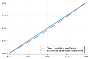
Figure 2: True Correlation vs. Estimated Correlation ($N_{E}=10$)

Note that whereas Kennan (2006) shows an “optimal” way of discretizing the support of a univariate random variable, we do not have such optimality result for a multivariate case. Thus, our approach should be understood as being heuristic.

B.1.1 Maximal Error from Discrete Approximation

Given that our approach relies on discrete approximations (as done in Syrgkanis, Tamer, and Ziani (2021) and Magnolfi and Roncoroni (forthcoming)), a natural question is how accurate the approximation is. We provide a simple numerical evidence which supports the claim that the approximation error is at most mild.

Consider a two-player entry game with payoff $u_{i}\left(a_{i},a_{j},\varepsilon_{i}\right)=a_{i}\left(\kappa_{i}a_{j}+\varepsilon_{i}\right)$. We generate observed choice probability data at $\left(\kappa_{1},\kappa_{2}\right)=\left(-0.5,-0.5\right)$ using a continuous distribution $\varepsilon_{i}\overset{\text{iid}}{\sim}N\left(0,1\right)$, and symmetric equilibrium selection probability. The population choice probability is $\left(\phi_{00},\phi_{01},\phi_{10},\phi_{11}\right)\approx\left(0.25,0.3274,0.3274,0.0952\right)$.

If we use the discrete approximation procedure described above, how much error can there be? Our measure of discrepancy is the solution to

$$\min_{t\in\mathbb{R},\sigma\in\Delta_{a|\varepsilon}}t\quad\text{subject to}$$

$$\sum_{\varepsilon_{-i}}\psi_{\varepsilon}\sigma_{a|\varepsilon}\partial u_{i}\left(\tilde{a}_{i},a,\varepsilon_{i}\right)\leq t,\quad\forall i,\varepsilon_{i},a,\tilde{a}_{i}$$

$$\sum_{\varepsilon}\psi_{\varepsilon}\sigma_{a|\varepsilon}-\phi_{a}\leq t,\quad\forall a$$

$$\phi_{a}-\sum_{\varepsilon}\psi_{\varepsilon}\sigma_{a|\varepsilon}\leq t,\quad\forall a$$

The solution $t^{*}$ measures the maximal relaxation required for the equilibrium conditions and the consistency conditions. If $t^{*}=0$, there is no approximation error. In general, we can expect $t^{*}>0$. Let $N_{E}$ be the number of grid points used for approximating $N\left(0,1\right)$. (We use $N_{E}=10$ for $\varepsilon_{1}$ and $\varepsilon_{2}$ in our empirical application which produces $10^{2}=100$ points for the support of $\psi$.)

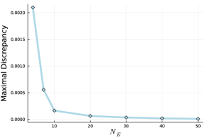
Figure 3: Discrete approximation error

Figure 3 plots $t^{*}$ (“maximal discrepancy”) against $N_{E}$. The figure shows that the discrepancy is decreasing in $N_{E}$ and at most modest after $N_{E}=10$. Since we construct confidence sets for the conditional choice probabilities when we do inference, it is likely that the approximation error will be controlled together. For this reason, it seems quite unlikely that discretization error will contaminate the estimation results.

B.2 Construction of Convex Confidence Sets for Conditional Choice Probabilities

In this section, we describe a simple approach to constructing confidence sets for the conditional choice probabilities, which we use for the empirical application. We construct simultaneous confidence intervals based on Fitzpatrick and Scott (1987). The basic idea is to construct confidence intervals for each multinomial proportion parameter so that the confidence set for the conditional choice probabilities can be characterized as a set of constraints that are linear in the population conditional choice probabilities. While there are many ways of constructing simultaneous confidence bands for a vector of means (e.g., see Olea and Plagborg-Møller (2019) and the references therein), we follow Fitzpatrick and Scott (1987) because it provides a very simple approach to constructing simultaneous confidence intervals for multinomial proportion parameters.

Let $\mathcal{X}$ be a finite set of covariates and $|\mathcal{X}|$ its cardinality. Let $\phi_{a}^{x}\in\mathbb{R}$ be the population choice probability of outcome $a\in\mathcal{A}$ at bin $x\in\mathcal{X}$. At each bin $x$, the conditional choice probabilities $\phi^{x}\equiv\left(\phi_{a}^{x}\right)_{a\in\mathcal{A}}\in\mathbb{R}^{|\mathcal{A}|}$ represent the proportion parameters of a multinomial distribution. The entire vector of conditional choice probabilities is denoted $\phi\equiv\left(\phi^{x}\right)_{x\in\mathcal{X}}\in\mathbb{R}^{|\mathcal{A}|\times|\mathcal{X}|}$. Let $n^{x}\in\mathbb{Z}$ be the number of observations at each bin $x$, and let $n\equiv\sum_{x\in\mathcal{X}}n^{x}$ be the total number of observations in the data.

Our strategy is described as follows. Our objective is to construct a confidence set $\Phi_{n}^{\alpha}$ that covers $\phi$ with probability at least $1-\alpha$ asymptotically where $\alpha\in\left(0,1\right)$. To do so, we will construct a confidence set $\Phi_{n^{x}}^{x,\beta_{\alpha}}$ at each bin $x$ that covers $\phi^{x}$ with probability at least $1-\beta_{\alpha}$ asymptotically where $\beta_{\alpha}=1-\left(1-\alpha\right)^{1/|\mathcal{X}|}$ ($\beta_{\alpha}$ arises from applying the Šidák correction for testing $|\mathcal{X}|$ number of independent hypotheses with family-wise error rate $\alpha$; note that the samples in each bin $x$ are independent from each other when the data are generated from independent markets). Next, we will construct $\Phi_{n}^{\alpha}$ by taking intersections of $\Phi_{n^{x}}^{x,\beta_{\alpha}}$ across $x$; making the coverage probability for $\phi^{x}$ at each $x$ be no less than $1-\beta_{\alpha}$ ensures that the overall coverage probability for $\phi$ is no less than $1-\alpha$. Moreover, if, for each $x$, $\Phi_{n^{x}}^{x,\beta_{\alpha}}$ can be represented by a set of constraints linear in $\phi^{x}$, then $\Phi_{n}^{\alpha}$ will be represented by a set of constraints linear in $\phi$ by construction.

At each $x\in\mathcal{X}$, we define the confidence set for $\phi^{x}$ as follows. Let $\hat{\phi}_{a}^{x}\equiv n_{a}^{x}/n^{x}\in\mathbb{R}$ be the nonparametric frequency estimator of $\phi_{a}^{x}$ where $n_{a}^{x}\in\mathbb{Z}$ is the number of observations with outcome $a$ at bin $x$. Then construct $\Phi_{n^{x}}^{x,\beta_{\alpha}}$ as:

$$\Phi_{n^{x}}^{x,\beta_{\alpha}}\equiv\left\{\phi^{x}:\ \phi_{a}^{x}\in\hat{\phi}_{a}^{x}\pm\frac{z\left(\beta_{\alpha}/4\right)}{2\sqrt{n^{x}}},\quad\forall a\in\mathcal{A}\right\},$$ (14)

where $z\left(\tau\right)\in\mathbb{R}$ denotes the upper $100\left(1-\tau\right)\%$ quantile of the standard normal distribution. Note that $\Phi_{n^{x}}^{x,\beta_{\alpha}}$ consists of $|\mathcal{A}|$ number of confidence intervals.

Finally, we define a confidence region for $\phi$ as:

$$\Phi_{n}^{\alpha}\equiv\left\{\phi:\ \phi^{x}\in\Phi_{n^{x}}^{x,\beta_{\alpha}},\quad\forall x\in\mathcal{X}\right\}.$$ (15)

The following proposition states that, under regular conditions, $\Phi_{n}^{\alpha}$ constructed as (15) has the desired asymptotic coverage probabilities for the population conditional choice probabilities $\phi$.

Proposition 1.

Let $\Phi_{n}^{\alpha}$ be defined as (15). Suppose that samples are independent across $x\in\mathcal{X}$, and $n^{x}\to\infty$ for each $x\in\mathcal{X}$ as $n\to\infty$. If $\alpha$ is sufficiently low or $|\mathcal{X}|$ is sufficiently large so that $\beta_{\alpha}\leq 0.032$, we have

$$\lim_{n\to\infty}\text{Pr}\left(\phi\in\Phi_{n}^{\alpha}\right)\geq 1-\alpha.$$

To prove Proposition 1, we use Theorem 1 of Fitzpatrick and Scott (1987) as a lemma. The lemma characterizes the asymptotic lower bounds on the coverage probabilities of $\Phi_{n^{x}}^{x,\beta_{\alpha}}$ for $\phi^{x}$ when the intervals of form (14) are used.

Lemma 2 (Fitzpatrick and Scott (1987) Theorem 1).

Let $\Phi_{n^{x}}^{x,\beta_{\alpha}}$ be defined as (14). Then

$$\lim_{n^{x}\to\infty}\text{Pr}\left(\phi^{x}\in\Phi_{n^{x}}^{x,\beta_{\alpha}}\right)\geq\mathcal{L}\left(\beta_{\alpha}\right)$$

where

$$\mathcal{L}\left(\beta_{\alpha}\right)=\begin{cases}1-\beta_{\alpha},&\text{if }\beta_{\alpha}\leq 0.032\\ 6\Phi\left(\frac{3z\left(\beta_{\alpha}/4\right)}{\sqrt{8}}\right)-5,&\text{if $0.032\leq\beta_{\alpha}\leq 0.3$}\end{cases}.$$

Now let us prove Proposition 1. The proof uses the fact that (i) the samples are independent across $x\in\mathcal{X}$, (ii) $\Phi_{n^{x}}^{x,\beta_{\alpha}}$ covers $\phi^{x}$ with probability no less than $\beta_{\alpha}$ asymptotically, and (iii) $\beta_{\alpha}$ is chosen in a way that ensures the overall coverage probability for $\phi$ becomes no less than $1-\alpha$ asymptotically (Šidak correction).

Proof.

We have

$$\text{Pr}\left(\phi\in\Phi_{n}^{\alpha}\right) =\text{Pr}\left(\phi^{x}\in\Phi_{n^{x}}^{x,\beta_{\alpha}},\quad\forall x\in\mathcal{X}\right)$$

$$=\prod_{x\in\mathcal{X}}\text{Pr}\left(\phi^{x}\in\Phi_{n^{x}}^{x,\beta_{\alpha}}\right)$$ (16)

where (16) follows from the independence across $x\in\mathcal{X}$. Given that $\beta_{\alpha}$ is sufficiently small, taking the limit gives

$$\lim_{n\to\infty}\prod_{x\in\mathcal{X}}\text{Pr}\left(\phi^{x}\in\Phi_{n^{x}}^{x,\beta_{\alpha}}\right) =\prod_{x\in\mathcal{X}}\lim_{n^{x}\to\infty}\text{Pr}\left(\phi^{x}\in\Phi_{n^{x}}^{x,\beta_{\alpha}}\right)$$ (17)

$$\geq\prod_{x\in\mathcal{X}}\left(1-\beta_{\alpha}\right)$$ (18)

$$=\left(1-\beta_{\alpha}\right)^{|\mathcal{X}|}$$

$$=\left(1-\left\{1-\left(1-\alpha\right)^{1/|\mathcal{X}|}\right\}\right)^{|\mathcal{X}|}$$ (19)

$$=1-\alpha.$$

where (17) follows from the product rule of limits, (18) follows from Fitzpatrick and Scott (1987) Theorem 1, and (19) follows from the definition of $\beta_{\alpha}$. ∎

The main advantage of using Fitzpatrick and Scott (1987) is its simplicity. The method is easily applicable even when there are zero count cells, i.e., $n_{a}^{x}=0$ for some $a\in\mathcal{A}$ and $x\in\mathcal{X}$. Zero count cells often occur when the sample size is small and may require some correction if other popular approaches (e.g., normal approximation for each $\phi_{a}^{x}$ taken as a Bernoulli parameter) were used. The simultaneous confidence bands can be conservative, but retains a linear structure, which is computationally attractive.

Example 4.

Suppose there are two bins $\mathcal{X}=\left\{l,h\right\}$, and that the number of observations at each bin is $n^{l}=400$ and $n^{h}=600.$ Suppose that $\mathcal{A}=\left\{00,01,10,11\right\}$ so that $\phi^{x}=\left(\phi_{00}^{x},\phi_{01}^{x},\phi_{10}^{x},\phi_{11}^{x}\right)$ and that we obtained $\hat{\phi}^{l}=\left(0.1,0.1,0.4,0.4\right)$ and $\hat{\phi}^{h}=\left(0.2,0.3,0.3,0.2\right)$ using nonparametric frequency estimators at each bin. If $\alpha=0.05$, then $\beta_{\alpha}=1-\left(1-\alpha\right)^{1/2}=0.0253$. Then $z\left(\beta_{\alpha}/4\right)=z\left(1-0.0253/4\right)=2.4931$. Finally, since $z\left(\beta_{\alpha}/4\right)/\left(2\sqrt{400}\right)=0.0623$ and $z\left(\beta_{\alpha}/4\right)/\left(2\sqrt{600}\right)=0.0509$, our $\Phi_{n}^{\alpha}$ is defined by the following inequalities:

$$\hat{\phi}_{a}^{l}-0.0623 \leq\phi_{a}^{l}\leq\hat{\phi}_{a}^{l}+0.0623,\quad\forall a\in\mathcal{A}$$

$$\hat{\phi}_{a}^{h}-0.0509 \leq\phi_{a}^{h}\leq\hat{\phi}_{a}^{h}+0.0509,\quad\forall a\in\mathcal{A}.$$

$\blacksquare$

B.2.1 Monte Carlo Experiment

We conduct Monte Carlo experiments to examine whether the simultaneous confidence bands have correct coverage probabilities and confirm that the approach works well. Let $\mathcal{X}=\left\{1,2,...,N_{\mathcal{X}}\right\}$ be a finite set indices (covariates). The following constitutes a single trial. We randomly generate a probability vector $\phi^{x}\in\mathbb{R}^{4}$ for $x=1,...,N_{\mathcal{X}}$ by taking a 4-dimensional uniform vector and normalize the vector so that it sums to one. Then, at each $x\in\mathcal{X}$, we generate a random sample by taking a draw from a multinomial distribution with parameter $\left(n^{x},\phi^{x}\right)$ where $n^{x}$ is the number trials. Finally, we test whether the simultaneous confidence bands, constructed as described above, covers $\phi^{x}$. We repeat this procedure for $100,000$ times and find the coverage probability.

Table 8: Coverage Probability of Simultaneous Confidence Bands from Simulation

	(A) $\alpha=0.05$						(B) $\alpha=0.01$
$N_{\mathcal{X}}\backslash n^{x}$	100	200	500	1000	10000		100	200	500	1000	10000
4	0.9697	0.9707	0.9713	0.9744	0.9837		0.9950	0.9948	0.9957	0.9956	0.9975
10	0.9735	0.9731	0.9748	0.9754	0.9854		0.9955	0.9954	0.9957	0.9960	0.9978
50	0.9760	0.9760	0.9777	0.9797	0.9885		0.9958	0.9962	0.9962	0.9968	0.9981
100	0.9779	0.9788	0.9791	0.9811	0.9886		0.9959	0.9961	0.9964	0.9969	0.9982
200	0.9776	0.9783	0.9794	0.9816	0.9902		0.9964	0.9962	0.9966	0.9971	0.9984

Table 8 reports the results of the Monte Carlo experiment. It shows that the confidence sets obtain desired coverage probabilities although they can be conservative. We conclude that the proposed approach works well.

B.3 Random Walk Surface Scanning Algorithm

Let $\Theta_{I}$ be the identified set of parameters. The identified set is defined as the level set

$$\Theta_{I}\equiv\left\{\theta\in\Theta:Q\left(\theta\right)\leq 0\right\}$$

where $Q\left(\theta\right)$ is a non-negative valued criterion function. (To obtain the confidence set, simply replace $Q\left(\theta\right)$ with $\widehat{Q}_{n}^{\alpha}\left(\theta\right)$.) Except for special cases (e.g., when $\Theta_{I}$ is convex), we need to approximate $\Theta_{I}$ by collecting a large number of points in $\Theta_{I}$. A naive approach is to conduct an extensive grid search: draw a fine grid on the parameter space $\Theta$ (e.g., by taking quasi-Monte Carlo draws) and evaluate the criterion function at all point on the grid. However, a naive grid search can be computationally burdensome especially when the dimension of $\theta$ is large.

In our setup, Theorem 8 says that we can get the gradient information for free due to the envelope theorem. That is, once we evaluate $Q\left(\theta\right)$ at any $\theta$, we can get $\nabla Q\left(\theta\right)$ as well. Exploiting the gradient information allows us to find a minimizer of $Q\left(\theta\right)$ far more efficiently because we can use gradient-based optimization algorithms (e.g., gradient descent or (L-)BFGS) as opposed to gradient-free algorithms. However, since we need to find all minimizers of $Q\left(\theta\right)$, solving $\min_{\theta}Q\left(\theta\right)$ is insufficient.

We propose a heuristic approach. First, we identify $\theta^{0}=\arg\min_{\theta}Q\left(\theta\right)$ by using a gradient-based optimization algorithm. Second, we iteratively explore the neighbors of the identified set by running a random walk process from $\theta^{0}$ and accepting points at which the criterion function is zero-valued. Being able to quickly identify a point in the identified set gives a considerable advantage over grid search algorithms because we do not have to explore points that are “far” from the identified set. The required assumption is that $\Theta_{I}$ is a connected set.

We use a random walk surface scanning algorithm described as follows. Let $\theta^{0}=\arg\min_{\theta}Q\left(\theta\right)$ be the identified parameter and assume that $Q\left(\theta^{0}\right)=0$ (otherwise the identified set is empty). From $\theta^{0}$, we take a random candidate

$$\tilde{\theta}^{1}\leftarrow\theta^{0}+\eta$$

where $\eta\sim N\left(0,\sigma_{\eta}^{2}\right)$ is a vector of random shocks. We then evaluate $Q\left(\tilde{\theta}^{1}\right)$ and check whether the value is equal to zero. If $Q\left(\tilde{\theta}^{1}\right)=0$, we accept the candidate $\tilde{\theta}^{1}$ and let $\theta^{1}\leftarrow\tilde{\theta}^{1}$. If $Q\left(\tilde{\theta}^{1}\right)>0$, then we draw a new $\tilde{\theta}^{1}$ until we find a point that is accepted. Iterating this process generates a random sequence of points $\theta^{0},\theta^{1},\theta^{2},...$ that “bounces” inside the level set $\Theta_{I}$. We iterate this process until we find a large number of points in $\Theta_{I}$.

To control the step size, we let $\sigma_{\eta}$ adjust adaptively. Specifically, if a candidate point is accepted, we increase $\sigma_{\eta}$ before a new draw is taken to make the search more aggressive. If a candidate point is rejected, we decrease $\sigma_{\eta}$ to make the search more conservative (a lower bound can be placed to prevent excessively small step size).

B.4 Counterfactual Analysis

In this section, we explain the implementation details for counterfactual analysis. Let us first lay out the counterfactual prediction problem. Let us call the game before and after the counterfactual policy pre-game and post-game respectively. Suppose we have a counterfactual policy that changes the pre-game $\left(G^{pre},S\right)$ to post-game $\left(G^{post},S\right)$ (we assume that a counterfactual policy only changes the payoff-relevant primitives, but not the information structure). In our application, we assume the counterfactual policy changes the covariates from $x^{pre}$ to $x^{post}$ so that the payoff function changes from $u_{i}^{pre}\left(a,\varepsilon_{i};\theta\right)\equiv u_{i}^{x^{pre},\theta}\left(a,\varepsilon_{i}\right)$ to $u_{i}^{post}\left(a,\varepsilon_{i};\theta\right)\equiv u_{i}^{x^{post},\theta}\left(a,\varepsilon_{i}\right)$. We assume that the prior distribution $\psi$ and the baseline information structure $S$ do not change.

Let $h:\mathcal{A}\times\mathcal{E}\to\mathbb{R}$ be the counterfactual objective of interest, which is a function of realized state of the world and action profiles (see examples provided below). At a fixed $x\in\mathcal{X}$, we can obtain the lower/upper bounds on the expected value of $h$ by finding the equilibria that will minimize/maximize the expected value of $h$:

$$\min/\max_{\sigma^{x}\in\Delta_{a|\varepsilon,t}}\sum_{\varepsilon,t,a}\psi_{\varepsilon}^{x}\pi_{t|\varepsilon}^{x}\sigma_{a|\varepsilon,t}^{x}h\left(a,\varepsilon\right)\quad\text{subject to }$$ (20)

$$\sum_{\varepsilon,t_{-i}}\psi_{\varepsilon}^{x}\pi_{t|\varepsilon}^{x}\sigma_{a|\varepsilon,t}^{x}\partial u_{i}^{x,\theta}\left(\tilde{a}_{i},a,\varepsilon\right)\leq 0,\quad\forall i,t_{i},a,\tilde{a}_{i}.$$

Note that (20) is a linear program.

We now connect the characterizations to the empirical application. Let $\mathcal{X}^{pre}$ be the set of covariates corresponding to the food deserts in Mississippi; there can be multiple values of $x^{pre}\in\mathcal{X}^{pre}$ because there are multiple markets with different observable covariates. By the definition of food deserts, all Mississippi food deserts have covariates with the low access to healthy food indicator equal to 1. For each market $m$, we define the counterfactual covariates as the vector obtained by changing the low access indicator from 1 to 0. For example, if $x^{pre}=\left(x^{highipc},x^{lowaccess}\right)=\left(1,1\right)$ for a particular market, we set $x^{post}=\left(1,0\right)$. This changes the game since the players’ payoff functions are changed. Then the set of covariates for the post-regime $\mathcal{X}^{post}$ is constructed by taking each $x^{pre}\in\mathcal{X}^{pre}$ and changing the low access indicator from 1 to 0.

We use four measures of market structure:

Counterfactual objective	$h\left(a,\varepsilon\right)$
Number of entrants	$1\times\left(\mathbb{I}\left\{a=\left(0,1\right)\right\}+\mathbb{I}\left\{a=\left(1,0\right)\right\}\right)+2\times\mathbb{I}\left\{a=\left(1,1\right)\right\}$
McDonald’s entry	$\mathbb{I}\left\{a=\left(1,0\right)\right\}+\mathbb{I}\left\{a=\left(1,1\right)\right\}$
Burger King entry	$\mathbb{I}\left\{a=\left(0,1\right)\right\}+\mathbb{I}\left\{a=\left(1,1\right)\right\}$
No entry	$\mathbb{I}\left\{a=\left(0,0\right)\right\}$

Suppose $\theta$ is given. At a fixed covariate $x$, we can obtain bounds on the expected value of $h$ by solving (20). However, since $\mathcal{X}^{pre}$ is non-singleton, we find the weighted average of the bounds. Let $\left\{w^{x}\right\}_{x\in\mathcal{X}^{pre}}$ be the weights at each covariate vector where $w^{x}$ is proportional to the number of markets corresponding to Mississippi food deserts in covariate bin $x\in\mathcal{X}^{pre}$; we scale the weights so that $\sum_{x\in\mathcal{X}^{pre}}w^{x}=1$. The weighted average on $h$ can be found by solving:

$$\min/\max_{\sigma}\sum_{x\in\mathcal{X}^{post}}w^{x}\sum_{\varepsilon,t,a}\psi_{\varepsilon}^{x}\pi_{t|\varepsilon}^{x}\sigma_{a|\varepsilon,t}^{x}h\left(a,x\right)\quad\text{subject to }$$

$$\sum_{\varepsilon,t_{-i}}\psi_{\varepsilon}^{x}\pi_{t|\varepsilon}^{x}\sigma_{a|\varepsilon,t}^{x}\partial u_{i}^{x,\theta}\left(\tilde{a}_{i},a,\varepsilon\right)\leq 0,\quad\forall x\in\mathcal{X}^{post},i,t_{i},a,\tilde{a}_{i}$$

$$\sigma^{x}\in\Delta_{a|\varepsilon,t},\quad\forall x\in\mathcal{X}^{post}$$

The bounds for the pre-counterfactual regime can be found by replacing $\mathcal{X}^{post}$ with $\mathcal{X}^{pre}$.

Finally, since $\Theta_{I}$ is set-valued, we repeat the above process for each $\theta$ in $\Theta_{I}$ and take the union of the bounds. Since there is a large number of points in $\Theta_{I}$, to save computation time, we use $k$-means clustering on $\Theta_{I}$ to find a set of points that approximate $\Theta_{I}$ (we choose $k$ equal to 2000 or larger and compare the projection of the original set to the projection of the approximating set to see if the approximation is accurate).

B.5 Overview of the Implementation

We provide a brief overview of how we obtain the confidence sets in the empirical application section. To prepare data for structural estimation, we use Stata to obtain discretized bins of covariates. We use estimate the conditional choice probabilities via nonparametric frequency estimator. We also compute the number of observations in each bin $x\in\mathcal{X}$ (which are inputs to constructing simultaneous confidence intervals for the CCPs) and define weights at each $x$ (which are inputs to criterion function) as being proportional to the number of observations. The final dataset has $|\mathcal{X}|$ rows, where each row contains vector of covariate values corresponding to bin $x$, CCP estimates $\hat{\phi}_{a}^{x}$ for each outcome $a\in\mathcal{A}$, and the number of observations at the covariate bin. We then export the data to Julia where all computations for structural estimation are done.

To prepare feasible optimization programs, we discretize the space of shocks using the approach described in Section B.1. We then declare optimization program using JuMP interface (Dunning et al., 2017). We construct the simultaneous confidence sets for the conditional choice probabilities using the approach described in B.2. This makes evaluation of the criterion functions $\widehat{Q}_{n}^{\alpha}\left(\theta\right)$ for each point $\theta\in\Theta$ a linear program. We use Gurobi to solve linear programs.

To approximate the confidence set $\widehat{\Theta}_{I}^{\alpha}$, we need to collect many points in $\Theta$ that satisfy the condition $\hat{Q}_{n}^{\alpha}\left(\theta\right)=0$. Collecting these points are done by the random walk surface scanning algorithm described in Section B.3. To use this approach, it is important to quickly identify an initial point $\theta^{0}$ such that $\hat{Q}_{n}^{\alpha}\left(\theta^{0}\right)=0$ by solving $\min_{\theta}\hat{Q}_{n}^{\alpha}\left(\theta\right)$. This can be done efficiently by using gradients of $\hat{Q}_{n}^{\alpha}\left(\theta\right)$ obtained by the envelope theorem (see Theorem 8). We recommend using many initial points to increase the chance of convergence, and decreasing the tolerance for optimality conditions ($\|\nabla\hat{Q}_{n}^{\alpha}\left(\theta\right)\|<\varepsilon^{tol}$) for higher accuracy. We use Knitro to solve nonlinear programs.

Specifically, we identify $\arg\min_{\theta}\hat{Q}_{n}^{\alpha}\left(\theta\right)$ by solving the minimization problem in two steps:

$$\min_{\theta}\hat{Q}_{n}^{\alpha}\left(\theta\right)=\min_{\theta^{\rho}}\left(\min_{\theta^{u}}\hat{Q}_{n}^{\alpha}\left(\theta^{u};\theta^{\rho}\right)\right)$$

where $\theta^{u}$ represent the parameters associated with the payoff functions and $\theta^{\rho}$ represent the correlation coefficient parameter for the distribution of payoff shocks. In the outer loop, we search for the minimum over a grid of $\theta^{\rho}$ on $\left[0,1\right]$. In the inner loop, taking $\theta^{\rho}$ as fixed, we solve $\min_{\theta^{u}}\hat{Q}_{n}^{\alpha}\left(\theta^{u};\theta^{\rho}\right)$ by minimizing (10) jointly with $\theta^{u}$. Solving the nested optimization program (the outer loop minimizes over $\theta^{u}$ and the inner loop minimizes over $q,\sigma,\phi$) as a single optimization program is faster when the number of variables is manageable; this is similar to the key idea of Su and Judd (2012). Although we can obtain $\psi^{x,\theta^{\rho}}$ in closed form so that the minimization problem can be solved jointly in $\left(\theta^{u},\theta^{\rho}\right)$, we chose to divide the minimization problem as above because $\psi^{x,\theta^{\rho}}$ can be highly non-linear in $\theta^{\rho}$.

Appendix C Data Appendix

This section describes the datasets used for our empirical application, which studies the entry game between McDonald’s and Burger King in the US. The following table provides an overview of the datasets used in this paper.

Dataset Name	Description
Data Axle (Infogroup) Historical Business Database	Proprietary; accessed via Wharton Research Data Services https://wrds-www.wharton.upenn.edu/ using institutional subscription. Data Axle (formerly known as Infogroup) is a data analytics marketing firm that provides digital and traditional marketing data on millions of consumers and businesses. Address-level records on business entities operating in the US are available for 1997-2019 at the annual level. We obtain the addresses of burger outlets in operation, which in turn are translated into tract-level entry decisions for each calendar year using the census shapefiles.
US Census Shapefiles	Accessible from https://www.census.gov/geographies/mapping-files/time-series/geo/tiger-line-file.html. Used to get 2010 census tract boundaries. Shapefiles are needed to find tract IDs corresponding to each physical store given their location coordinates.
Longitudinal Tract Data Base (LTDB)	Accessible from https://s4.ad.brown.edu/projects/diversity/researcher/bridging.htm. LTDB provides tract-level demographic information (from the census) for 1970-2010 harmonized to 2010 tract boundaries. We obtain population and income per capita for year 2000 and 2010 from here.
National Neighborhood Data Archive (NaNDA)	Accessible from https://www.openicpsr.org/openicpsr/nanda. NaNDA provides measures of business activities at each tract. We obtain the number of eating and drinking places for year 2010 at the tract level. Other variable such as the number of grocery stores (per square miles), the number of super-centers, and the number of retail stores are available.
Food Access Research Atlas	Accessible from https://www.ers.usda.gov/data-products/food-access-research-atlas/. Food Access Research Atlas provides information on whether a census tract has limited access to supermarkets, super-centers, grocery stores, or other sources of healthy and affordable food. We obtain indicators for “low access to healthy food” and “food deserts” at the tract level for year 2010. A census tract is classified as a food desert if it is identified as having low access to healthy food and low income. A census tract is classified as low-access tract if at least 500 people or at least 33 percent of the population is greater than 1/2 mile from the nearest supermarket, supercenter, or large grocery store for an urban area or greater than 10 miles for a rural area. The criteria for identifying a census tract as low-income are from the Department of Treasury’s New Markets Tax Credit (NMTC) program.

C.1 Data Construction

We merge multiple datasets to construct the final sample used for structural estimation. The details are described as follows.

Panel data at tract-year level

Although we use 2010 cross-section for estimation of the structural model, we construct a panel dataset at a tract-year level to track the openings and closings of fast-food outlets in the US. We make the sample period run from 1997 to 2019, corresponding to the period for which business location data from Data Axle Historical Business Database are available.

We define the units for markets as 2010 census tracts designated by the US Census Bureau. (We define potential markets as 2010 urban tracts. See below for the definition of urban tracts.) Year 2010 was selected since it was the latest year for which the decennial census data was available when we started the empirical analysis. For all years in the sample period, we fix markets as 2010 census tracts; although census tract boundaries change slightly every decade, we fixed the boundaries for consistency across time.

To construct tract-level data, we first download the 2010 census shapefiles from the US Census to obtain the list of all 2010 census tracts (there are 74,134 tracts defined for the 2010 decennial census in the US and its territories). Next, we exclude all tracts outside the contiguous US: Alaska, Hawaii, American Samoa, Guam, Northern Mariana Islands, Puerto Rico, and the Virgin Islands. We drop these regions since the data generating process (specifically how the game depends on observable market characteristics) is likely to differ from the rest.

Using the market-year panel data as a “blank sheet”, we append relevant variables that include the firms’ entry decisions in each tract for a given year and observable tract characteristics such as population. At this stage, we can create a variable distance to headquarter by measuring the distance between the location of a firm’s headquarter and the centroid of a tract (McDonald’s and Burger King have their headquarters in Chicago and Florida respectively).

In the final dataset used for the empirical application, we restrict attention to 2010 urban census tracts (i.e., we drop all rural tracts). A census tract is defined as urban if its population-weighted centroid is in an “urban area” as defined in the Census Bureau’s urbanized area definition; a census tract is rural if not urban. We obtain the urban tract indicator from the Food Access Research Atlas.

Coding Entry Decisions

The primary source of data for our empirical application is Data Axle’s Historical Business Database. The dataset contains the list of local business establishments operating in the US over 1997-2019 at an annual level. Each establishment is assigned a unique identification number which can be used to construct establishment-level panel data. In addition, the dataset contains information such as company name, parent company, location of the establishment in coordinates, number of employees, industry codes.

We first need to download the entire list of burger outlets that were in operation. We download raw data from Wharton Research Data Services (WRDS) using the qualifier “SIC code=58” (retail eating places). We then identify relevant burger chains using company (brand) names and their parent number. In principle, each burger chain should have a unique parent number by the data provider. For example, all McDonald’s outlets have parent number “001682400”. Ideally, one can identify all burger chains that belong to a brand using their names and parent numbers. However, there are some errors due to misclassifications, which makes identifying all relevant burger chains more difficult. For example, McDonald’s outlets will have different company names such as “MC DONALD’S”, “MCDONALDS”, and “MC DONALD”. In addition, some McDonald’s outlets have parent numbers missing for some subset of years, or some establishments have duplicate observations.

To overcome this issue, we rely on the coordinates information to identify unique establishments. Since the same establishment can have different coordinates assigned over time depending on which point of place is used to measure the coordinates, we put each establishment in blocks approximately 250 meters in height and width. The idea is to put all observations whose coordinates are very close to each other in a single bin. Then we assign a unique establishment id to the stores in each block, i.e., we treat them as corresponding to a single store. We find that while it is challenging to avoid minor classification errors, the total number of burger chains outlets identified by our procedure closely is very close to the total number of outlets reported by other sources (e.g., reports in Statista https://www.statista.com/). Identifying unique establishments allows the construction of establishment-level panel data, which can be used to track firm entries and exits in each market.

The final step is to reshape the establishment-level panel data to market-level data to tabulate the number of burger chains operating in each market-year pair. We accomplish this with the help of Stata’s geocoding function, which helps identify census tract id’s corresponding to each coordinate (location of establishments). We then tabulate the number of outlets by each brand at a year-tract level.

In each market, we code entry decisions as binary variables. There were very few cases of a firm having more than one outlet in a single tract (approximately 1.5% of markets for McDonald’s and 0.3% for Burger King). We also construct a firm-specific variable own outlets in nearby markets. This variable records the number of own-brand outlets operating in adjacent markets (neighboring markets that share the same borders). For example, if for market $m$, McDonald’s nearby outlets are 2, it means that there were a total of 2 outlets operating in markets adjacent to market $m$. We constructed this variable with the help of a dataset downloaded from Diversity and Disparities project website that provides the list of 2010 census tracts and adjacent tracts.

Market Characteristics

We obtain tract-level characteristics from multiple sources described in the table above. All of these datasets provide variables at tract-level for the year 2010. We append tract-level characteristics to the main dataset that has entry decisions and firm-specific variables at tract-level.

Appendix D Adjustment Costs

D.1 Adjustment Costs in the Model

Throughout the paper, we have assumed that adjustment costs (e.g., sunk entry costs) are zero. The assumption is very common for static entry models (see, e.g., Bresnahan and Reiss (1990; 1991b), Ciliberto and Tamer (2009), Ciliberto and Jäkel (2021), Ciliberto et al. (2021), and Magnolfi and Roncoroni (forthcoming)). The assumption is also commonly used in other econometric frameworks, e.g., matching, network formation, and consumer choice. Whether the zero-adjustment costs assumption is appropriate or realistic depends on the research question, empirical setting, and the empirical model. If the researcher believes that adjustment costs (might) drive the observed decisions, then the researcher should model the adjustment costs. For instance, adjustment costs may play an important role in firms’ decision timings in a dynamic model. However, in static entry games, static profit functions are often interpreted as a reduced-form representation of long-run profit associated with the firms’ decisions. In this case, one-time sunk payment associated with changing the operating status (e.g., from “staying out” to “staying in”) is likely to be small relative to long-run profit. Although adjustment costs can be introduced in the model, the zero-adjustment costs assumption helps us motivate the main topic of this paper and simplify the exposition. Finally, we remark that we cannot identify adjustment costs with typical cross-sectional data that do not provide information on how firms switched from one state to another.

We note that our main results up to the econometrics section are not affected by the zero-adjustment costs assumption. If there are adjustment costs, then we can treat the realized action profile as a state variable and introduce adjustment costs as a function of a player’s current action and new action. Introducing adjustment costs do not affect the form of outcome functions, which serve as players’ model of the relationship between signal profiles and outcomes. Thus, the definition of rational expectations equilibrium is unaffected; the presence of adjustment costs only makes deviation from the realized outcome more difficult. The relationship between Bayes stable equilibrium and rational expectations equilibrium (Theorem 1) also remains intact. However, it should be clear that introducing adjustment costs in a static model requires assumptions about the timing and speed of firms’ actions as well as the size of the adjustment costs relative to long-run profits. Also note that an outcome function would be silent on how the players reached a certain outcome in the presence of adjustment costs.

D.2 Adjustment Costs in the Fast-Food Industry

In the empirical section, we assume that the burger chains can revise their actions costlessly. One-time sunk costs incurred for revising a decision (from “in” to “out” or vice versa) are likely negligible relative to the discounted sum of payoffs over long horizon, especially when the one-time payments are not significant and firms tend to adhere to a certain decision for a long period. In fact, the one-time payments associated with adjusting the operating status of a restaurant seem non-significant in the fast-food industry.

When a fast-food outlet opens or closes, the store has to incur one-time sunk costs that would not be incurred in the absence of adjustments. For example, a store that is opening has to pay legal fees for obtaining licenses to operate a restaurant. A store that intends to close might be constrained by terms of contract at least in the short run. The total amount of adjustment costs varies, but our investigation of fast-food restaurants suggests that adjustment costs are generally small relative to the long-run profits in the industry. While the details of the cost structure of McDonald’s and Burger King are proprietary, their franchise disclosure documents provide a rough idea of the relative magnitude of sunk entry costs. The 2021 McDonald’s Franchise Disclosure Document (FDD) reports that the average annual sales volume of domestic (US) traditional McDonald’s restaurants was $3,487,000 (the average profit per store is not reported since rents vary considerably depending on the outlet’s location). Operating expenses include food costs, labor costs, rent/lease, loan payments, equipment leases, fixed salaries, taxes, advertising fee, promotion, utilities, insurance, office supplies/postage/shipping, etc. A typical opening costs for a restaurant include those for construction, remodeling, licenses/permits, and professional/legal services. The FDD reports that expenses on signs, seating, equipment, and decor typically ranges between $1,000,000 and $1,600,000. However, a subset of these expenses is not sunk as they include purchase of capital that can be resold or used in other outlets. Exit costs are less well-documented. However, when a fast-food restaurant decides to close, it is likely that land, buildings, equipment and furniture can be sold at a fair market value or used in other outlets. Thus, it seems reasonable to assume that adjustment costs do not play an important role in shaping firms’ long run decision.

The profit function parameter estimates from Aguirregabiria and Magesan (2020) also support our assumption that the adjustment costs are negligible. In their empirical application, they study the dynamic entry game played by McDonald’s and Burger King in the UK during the period 1991–1995. The estimates of structural payoff parameters, reported in Table 9 of their paper, show that the sunk entry costs are small relative to the estimated annual variable profits, implying that sunk entry costs are likely to be negligible in the long run. They do not estimate exit costs because there were no exists during the period they study.

Appendix E Outcome Functions

Rational expectations equilibrium assumes that players refine their information via a commonly agreed outcome function. In this section, we further examine the role of outcome functions by allowing each player to hold a different outcome function and studying the implications. We discuss minimal conditions that must be imposed on outcome functions in equilibrium and how outcome functions relate to players’ ability to process information.

E.1 The Role of Outcome Functions

In the baseline version of the rational expectations equilibrium, it is assumed that all players agree on a single outcome function $\delta:\mathcal{T}\to\Delta\left(\mathcal{A}\right)$. In this case, $\delta$ plays multiple roles. First, $\delta$ represents the true data generating process in a reduced form. While the model is silent on how $\delta$ comes about, the use of $\delta$ reflects the fact that some relationship between exogenous signals and endogenous outcomes exists. Second, $\delta$ represents players’ subjective model of how signals relate to actions. The rational expectations equilibrium assumes that players’ models are correct. Third, $\delta$ represents players’ information updating rule. Each player use $\delta$ to assess if deviation from a given outcome can be profitable. Clearly, such assumption on information updating is strong as it ignores how the players might have updated their information along the interaction process before stable actions are determined and realized, but it substantially simplifies the characterization of the equilibrium.

E.2 Heterogeneous Outcome Functions

Relaxing the symmetry assumption and allowing players to hold heterogenous outcome functions disentangles the roles. Suppose that each player $i$ uses outcome function $\delta_{i}:\mathcal{T}\to\Delta\left(\mathcal{A}\right)$. Each $\delta_{i}$ represents $i$’s subjective model of how players’ information relates to market outcomes. We maintain the “rational expectations” assumption—that each player refines her information after observing $a$ using Bayes’ rule with $\delta_{i}$—since the players can observe opponents’ actions at stable outcomes. However, we relax the baseline assumption that $\delta_{i}$’s be identical across players.

E.2.1 Data Generating Process

To say that $\delta_{i}$ is correct or incorrect requires reference to the true data generating process, so we need to introduce $\delta^{*}:\mathcal{T}\to\Delta\left(\mathcal{A}\right)$ to denote the true data generating process. Each $\delta_{i}$ represents player $i$’s subjective model, whereas $\delta^{*}$ represents the objective model. If $\delta_{i}\neq\delta^{{}^{*}}$, then player $i$’s model is misspecified.

E.2.2 Minimal Consistency Requirements

Although $\delta_{i}$’s are subjective, any reasonable notion of equilibrium will require that $\delta_{i}$’s cannot be too arbitrary. First, we should require that $\delta_{i}$’s generate no deviation incentives. This requires evaluating whether $i$ finds deviation incentives at every information set that can be realized with positive probability under $\delta^{*}$. Second, a player’s subjective belief cannot contradict information available at equilibrium. The true data generating process $\delta^{*}$ should be consistent with the actual behavior induced by $\delta_{i}$’s. Moreover, the empirical distribution over a player’s information set should be consistent with the distribution implied by $\delta_{i}$ since the player can detect inconsistency otherwise. Complete characterization of the equilibrium conditions with heterogeneous beliefs depends on the analyst’s assumptions, but it is clear that any reasonable concept of equilibrium will constrain players’ subjective beliefs from being too arbitrary because rational players will use information available at equilibrium to refine their beliefs.

E.2.3 Processing Information

In rational expectations equilibrium, $\delta_{i}$ represents a channel through which player $i$ refines her information upon observing market outcomes. Given that $\delta_{i}$ is subjective, it is natural to ask whether $\delta_{i}$’s can be used to reflect differences in the ability to process information. For example, can we capture differences in McDonald’s and Burger King’s ability to process information by setting $\delta_{i}$’s appropriately? It turns out that this is quite difficult because the model imposes minimal level of sophistication on players, which in turn constrains $\delta_{i}$’s from being too arbitrary in equilibrium. While the analyst may consider setting $\delta_{i}$ so as to mimic limited ability to update information (e.g., by setting $\delta_{i}:\mathcal{T}\to\Delta\left(\mathcal{A}\right)$ to a constant function or controlling the degree of misspecification), such approach is constrained by the consistency requirements discussed above (i.e., that $\delta_{i}$ cannot contradict what $i$ can observe or learn in equilibrium). Thus, in the rational expectations equilibrium framework, the assumptions on players’ rationality limits the analyst’s freedom in manipulating $\delta_{i}$ to capture potential heterogeneity in players’ ability to process information.

References

- Aguirregabiria and Jeon (2020) Aguirregabiria, V. and J. Jeon (2020): “Firms’ Beliefs and Learning: Models, Identification, and Empirical Evidence,” Review of Industrial Organization, 56, 203–235.
- Aguirregabiria and Magesan (2020) Aguirregabiria, V. and A. Magesan (2020): “Identification and Estimation of Dynamic Games When Players’ Beliefs Are Not in Equilibrium,” The Review of Economic Studies, 87, 582–625.
- Aizawa and Fang (2020) Aizawa, N. and H. Fang (2020): “Equilibrium Labor Market Search and Health Insurance Reform,” Journal of Political Economy, 128, 4258–4336.
- Allcott et al. (2019) Allcott, H., R. Diamond, J.-P. Dubé, J. Handbury, I. Rahkovsky, and M. Schnell (2019): “Food Deserts and the Causes of Nutritional Inequality,” The Quarterly Journal of Economics, 134, 1793–1844.
- Aradillas-Lopez (2010) Aradillas-Lopez, A. (2010): “Semiparametric estimation of a simultaneous game with incomplete information,” Journal of Econometrics, 157, 409–431.
- Aradillas-López (2020) Aradillas-López, A. (2020): “The Econometrics of Static Games,” Annual Review of Economics, 12, 135–165.
- Aradillas-Lopez and Rosen (2022) Aradillas-Lopez, A. and A. M. Rosen (2022): “Inference in ordered response games with complete information,” Journal of Econometrics, 226, 451–476.
- Aradillas-Lopez and Tamer (2008) Aradillas-Lopez, A. and E. Tamer (2008): “The Identification Power of Equilibrium in Simple Games,” Journal of Business & Economic Statistics, 26, 261–283.
- Bajari et al. (2010a) Bajari, P., H. Hong, J. Krainer, and D. Nekipelov (2010a): “Estimating Static Models of Strategic Interactions,” Journal of Business & Economic Statistics, 28, 469–482.
- Bajari et al. (2010b) Bajari, P., H. Hong, and S. P. Ryan (2010b): “Identification and Estimation of a Discrete Game of Complete Information,” Econometrica, 78, 1529–1568.
- Beresteanu et al. (2011) Beresteanu, A., I. Molchanov, and F. Molinari (2011): “Sharp Identification Regions in Models With Convex Moment Predictions,” Econometrica, 79, 1785–1821.
- Bergemann and Morris (2013) Bergemann, D. and S. Morris (2013): “Robust Predictions in Games With Incomplete Information,” Econometrica, 81, 1251–1308.
- Bergemann and Morris (2016) ——— (2016): “Bayes correlated equilibrium and the comparison of information structures in games,” Theoretical Economics, 11, 487–522.
- Bergemann and Morris (2017) ——— (2017): “Belief-free rationalizability and informational robustness,” Games and Economic Behavior, 104, 744–759.
- Boyd and Vandenberghe (2004) Boyd, S. and L. Vandenberghe (2004): Convex optimization, Cambridge: Cambridge university press.
- Bresnahan and Reiss (1990) Bresnahan, T. F. and P. C. Reiss (1990): “Entry in Monopoly Markets,” The Review of Economic Studies, 57, 531.
- Bresnahan and Reiss (1991a) ——— (1991a): “Empirical models of discrete games,” Journal of Econometrics, 48, 57–81.
- Bresnahan and Reiss (1991b) ——— (1991b): “Entry and competition in concentrated markets,” Journal of Political Economy, 99, 977–1009.
- Canay and Shaikh (2017) Canay, I. A. and A. M. Shaikh (2017): “Practical and Theoretical Advances in Inference for Partially Identified Models,” in Advances in Economics and Econometrics: Eleventh World Congress, ed. by B. Honoré, A. Pakes, M. Piazzesi, and L. Samuelson, Cambridge: Cambridge University Press, vol. 2 of Econometric Society Monographs, chap. 9, 271–306.
- Chernozhukov et al. (2007) Chernozhukov, V., H. Hong, and E. Tamer (2007): “Estimation and Confidence Regions for Parameter Sets in Econometric Models,” Econometrica, 75, 1243–1284.
- Chiappori and Salanié (2016) Chiappori, P.-A. and B. Salanié (2016): “The Econometrics of Matching Models,” Journal of Economic Literature, 54, 832–861.
- Ciliberto and Jäkel (2021) Ciliberto, F. and I. C. Jäkel (2021): “Superstar exporters: An empirical investigation of strategic interactions in Danish export markets,” Journal of International Economics, 129, 103405.
- Ciliberto et al. (2021) Ciliberto, F., C. Murry, and E. Tamer (2021): “Market Structure and Competition in Airline Markets,” Journal of Political Economy, 129, 2995–3038.
- Ciliberto and Tamer (2009) Ciliberto, F. and E. Tamer (2009): “Market Structure and Multiple Equilibria in Airline Markets,” Econometrica, 77, 1791–1828.
- de Paula (2013) de Paula, Á. (2013): “Econometric Analysis of Games with Multiple Equilibria,” Annual Review of Economics, 5, 107–131.
- De Paula (2020) De Paula, Á. (2020): “Econometric models of network formation,” Annual Review of Economics, 12, 775–799.
- Doval and Ely (2020) Doval, L. and J. C. Ely (2020): “Sequential Information Design,” Econometrica, 88, 2575–2608.
- Draganska et al. (2008) Draganska, M., S. Misra, V. Aguirregabiria, P. Bajari, L. Einav, P. Ellickson, D. Horsky, S. Narayanan, Y. Orhun, P. Reiss, K. Seim, V. Singh, R. Thomadsen, and T. Zhu (2008): “Discrete choice models of firms’ strategic decisions,” Marketing Letters, 19, 399–416.
- Dunning et al. (2017) Dunning, I., J. Huchette, and M. Lubin (2017): “JuMP: A modeling language for mathematical optimization,” SIAM Review, 59, 295–320.
- Einav (2010) Einav, L. (2010): “Not All Rivals Look Alike: Estimating an Equilibrium Model of the Release Date Timing Game,” Economic Inquiry, 48, 369–390.
- Ellickson and Misra (2011) Ellickson, P. B. and S. Misra (2011): “Structural workshop paper—Estimating discrete games,” Marketing Science, 30, 997–1010.
- Fitzpatrick and Scott (1987) Fitzpatrick, S. and A. Scott (1987): “Quick Simultaneous Confidence Intervals for Multinomial Proportions,” Journal of the American Statistical Association, 82, 875–878.
- Fudenberg and Levine (1993) Fudenberg, D. and D. K. Levine (1993): “Self-Confirming Equilibrium,” Econometrica, 61, 523–545.
- Galichon and Henry (2011) Galichon, A. and M. Henry (2011): “Set Identification in Models with Multiple Equilibria,” The Review of Economic Studies, 78, 1264–1298.
- Gayle and Luo (2015) Gayle, P. G. and Z. Luo (2015): “Choosing between Order-of-Entry Assumptions in Empirical Entry Models: Evidence from Competition between Burger King and McDonald’s Restaurant Outlets,” The Journal of Industrial Economics, 63, 129–151.
- Goll (2000) Goll, D. (2000): “Seattle’s ’other’ coffee giant moves in,” The Business Journals.
- Green and Laffont (1987) Green, J. R. and J.-J. Laffont (1987): “Posterior Implementability in a Two-Person Decision Problem,” Econometrica, 55, 69–94.
- Grieco (2014) Grieco, P. L. E. (2014): “Discrete games with flexible information structures: an application to local grocery markets,” The RAND Journal of Economics, 45, 303–340.
- Gualdani and Sinha (2020) Gualdani, C. and S. Sinha (2020): “Identification and inference in discrete choice models with imperfect information,” arXiv:1911.04529 [econ], arXiv: 1911.04529.
- Ho and Rosen (2017) Ho, K. and A. M. Rosen (2017): “Partial Identification in Applied Research: Benefits and Challenges,” in Advances in Economics and Econometrics: Eleventh World Congress, ed. by B. Honoré, A. Pakes, M. Piazzesi, and L. Samuelson, Cambridge: Cambridge University Press, vol. 2 of Econometric Society Monographs, chap. 10, 307–359.
- Horowitz and Lee (forthcoming) Horowitz, J. L. and S. Lee (forthcoming): “Inference in a class of optimization problems: Confidence regions and finite sample bounds on errors in coverage probabilities,” Journal of Business and Economic Statistics.
- Igami and Yang (2016) Igami, M. and N. Yang (2016): “Unobserved heterogeneity in dynamic games: Cannibalization and preemptive entry of hamburger chains in Canada,” Quantitative Economics, 7, 483–521.
- Kalai (2004) Kalai, E. (2004): “Large Robust Games,” Econometrica, 72, 1631–1665.
- Kennan (2006) Kennan, J. (2006): “A Note on Discrete Approximations of Continuous Distributions,” Unpublished Manuscript. URL: https://www.ssc.wisc.edu/~jkennan/research/DiscreteApprox.pdf (Last accessed: October 2021).
- Kennan and Walker (2011) Kennan, J. and J. R. Walker (2011): “The Effect of Expected Income on Individual Migration Decisions,” Econometrica, 79, 211–251.
- Kline (2015) Kline, B. (2015): “Identification of complete information games,” Journal of Econometrics, 189, 117–131.
- Kline and Tamer (2016) Kline, B. and E. Tamer (2016): “Bayesian inference in a class of partially identified models,” Quantitative Economics, 7, 329–366.
- Kolb (2021) Kolb, K. H. (2021): Retail Inequality: Reframing the Food Desert Debate, Univ of California Press.
- Lee and Seshadri (2019) Lee, S. Y. T. and A. Seshadri (2019): “On the Intergenerational Transmission of Economic Status,” Journal of Political Economy, 127, 855–921.
- Leung (2003) Leung, S. (2003): “A Glutted Market Is Leaving Food Chains Hungry for Sites: Finding Spots for New Outlets Takes Heaps of Research, an Eye for Details,” The Wall Street Journal.
- Liu (2020) Liu, Q. (2020): “Stability and Bayesian Consistency in Two-Sided Markets,” American Economic Review, 110, 2625–2666.