pyspeckit: A spectroscopic analysis and plotting package

Abstract

pyspeckit is a toolkit and library for spectroscopic analysis in Python. We describe the pyspeckit package and highlight some of its capabilities, such as interactively fitting a model to data, akin to the historically widely-used splot function in IRAF. pyspeckit employs the Levenberg-Marquardt optimization method via the mpfit and lmfit implementations, and important assumptions regarding error estimation are described here. Wrappers to use pymc and emcee as optimizers are provided. A parallelized wrapper to fit lines in spectral cubes is included. As part of the astropy affiliated package ecosystem, pyspeckit is open source and open development and welcomes input and collaboration from the community.

1 Introduction and Background

Spectroscopy is an important tool for astronomy. Spectra are represented as the number of photons, or total energy in photons, arriving over a specified wavelength (or equivalently, frequency or energy) range. Emission and absorption lines caused by transitions between states in ions, atoms, and molecules bear important information in their observed intensity, width, and velocity centroid. These parameters are typically measured from model fits to the data, such as Gaussian, Lorentzian, and Voigt profiles. Historically, IRAF (Tody, 1986) provided the astronomy community with easy-to-use tools for line fitting, but IRAF development has mostly ceased in the last several years. The lack of an equivalent available tool in Python prompted the creation of pyspeckit.

pyspeckit development began in 2009 with a script called ‘showspec’ in the agpy package hosted on Google Code. It was created and used by a graduate student to plot and sometimes fit profiles to spectra in python. At the time, IDL was still more popular than python at most institutes (the first evidence that python had overtaken IDL in popularity among astronomers was presented in Momcheva & Tollerud, 2015), and there were no publicly available and advertised tools for spectral plotting, fitting, and general manipulation (astropysics, Tollerud 2012, was developed contemporaneously and solved many of the same problems as pyspeckit). The astropy package (Astropy Collaboration et al., 2013, 2018) had its first commit in 2011, so even the basic infrastructure for such analysis was not yet established.

pyspeckit’s graphical user interface (GUI) features were inspired by IRAF’s splot tool, while the fitting features were inspired in part by xspec (https://heasarc.gsfc.nasa.gov/xanadu/xspec/). Over subsequent years, pyspeckit grew by incorporating more sophisticated models and improving its internal structure. The package was moved out of agpy and into its own repository in 2011, first spending a few years on Bitbucket in a mercurial repository, then finally moved to GitHub in 2012, where it currently resides (https://github.com/pyspeckit/pyspeckit/). Release v1.0 is available on Zenodo (Ginsburg et al., 2022).

Because pyspeckit’s initial development preceded astropy, some features were included that later became redundant with astropy. Most notably, pyspeckit included a limited system for spectroscopic unit conversion. In 2015, this system was completely replaced with astropy’s unit system. Around the same time, the Doppler conversion tools (converting from frequency or wavelength to velocity) that existed in pyspeckit were pushed upstream into astropy, highlighting the mutually beneficial role of astropy’s affiliated packaged system (Astropy Collaboration et al., 2018). pyspeckit became an astropy affiliated package in 2017 (An affiliated package is an astronomy-related Python package that is not part of the astropy core package, and is not managed by the project but is a part of the Astropy Project community).

In this paper we briefly outline pyspeckit’s architecture and highlight its key capabilities. In Section 2, we outline the structure of the package. In Section 3, we describe the GUI system. In Sections 4 and 5, we outline pyspeckit’s cube handling capabilities and model library. The appendices describe parameter error estimation for Gaussians (Appendix A) and for the ammonia model B). Appendix C describes a benchmarking test of the N₂H+ model against the CLASS version. Appendix D describes a framework for local-thermodynamic-equilibrium-based multi-transition modeling. Finally, Appendix E describes the integration of pyspeckit into ScousePy.

2 Package structure

The central object in pyspeckit is a Spectrum, which has associated data (e.g., flux), error (assumed to be symmetric, 1$\sigma$, Gaussian uncertainty), and xarr (e.g., wavelength, frequency, energy), the latter of which represents the spectroscopic axis. A Spectrum object has several attributes that are themselves classes that can be called as functions: the plotter, the fitter specfit, and the continuum fitter baseline.

There are several subclasses of Spectrum: Spectra is a collection of spectra intended to be stitched together (i.e., with non-overlapping spectral axes, e.g., for Echelle spectra), ObsBlock is a collection of spectra with identical spectral axes intended to be operated on as a group, e.g., to take an average spectrum, and Cube is a 3D spatial-spatial-spectral cube.

2.1 Supported data formats

pyspeckit supports a variety of open and proprietary data formats that have been traditionally used to store spectroscopic data products in astronomy. It is always possible to create a Spectrum object from numpy (van der Walt et al., 2011; Harris et al., 2020) arrays representing the wavelength, flux, and error of the spectrum, but the supported file formats listed below make the reading process easier.

• ASCII: Text files with wavelength, flux, and optional error columns can be read using the astropy.io.ascii module.

• FITS: The Flexible Image Transport System (FITS; Wells et al., 1981; Greisen et al., 2006; Pence et al., 2010) format is supported in pyspeckit with astropy.io.fits. FITS spectra are expected to have their spectral axis defined using the WCS keywords in the FITS header. FITS binary tables with the same wavelength, flux, and optional error column layout as text files can also be read.

• SDFITS: Data files following the Single Dish FITS (SDFITS; Garwood, 2000) convention for radio astronomy data as produced by the Green Bank Telescope are partly supported in pyspeckit.

• HDF5: If the h5py package is installed, pyspeckit will support read access to files containing spectra in the HDF5 format, where the data columns can be specified using keyword arguments.

• CLASS: pyspeckit is capable of reading files from some versions of the GILDAS Continuum and Line Analysis Single-dish Software format (CLASS; Gildas Team, 2013). The CLASS reader has been tested with data files from the Arizona Radio Observatory telescopes (12-m and 10-m Submillimeter Telescope) and the Atacama Pathfinder Experiment (APEX) radio telescope.

2.2 Plotter

The plotter is a basic plot tool that comprises pyspeckit’s main graphical user interface. It is described in more detail in the GUI section (§3).

2.3 Fitter

The fitting tool in pyspeckit is the Spectrum.specfit object. This object is a class that is created for every Spectrum object. The fitter can be used with any of the models included in the model registry, or a custom model can be created and registered.

To fit a profile to a spectrum, several optimizers are available. Two implementations of the Levenberg-Marquardt optimization method (Levenberg, 1944; Marquardt, 1963) are provided, mpfit and lmfit (Newville et al., 2014). Wrappers of pymc (Salvatier et al., 2016) and emcee are also available, though these tools are better for parameter error analysis than for optimization.

Once a fit is performed, the results of the fit are accessible through the parinfo object, which is a dictionary-like structure containing the parameter values, errors, and other metadata (e.g., information about whether the parameter is fixed, tied to another parameter, or limited). Other information about the fit, such as the $\chi^{2}$ value, are available as attributes of the specfit object.

Optimal $\chi^{2}$

Specfit computes the ‘optimal’ $\chi^{2}$, which is the $\chi^{2}$ value computed only over the range where the model contains statistically significant signal. This measurement is intended to provide a more accurate estimate of the $\chi^{2}$ value by excluding pixels that are not described by the model. By default, the function selects all pixels where the model value is greater (in absolute value) than the corresponding error. In principle, this optimal $\chi^{2}$ may be helpful for obtaining correctly scaled errors (see Section 2.6.1), though this claim has never been rigorously tested.

2.4 Data Selection

An important feature of the spectral fitter is the ability to select the region of the spectrum to be fit. This selection process can either be done manually, using the selectregion method to set one or more ranges of data to include in the fit, or interactively using the GUI. The selected regions are then highlighted in the plot window if one is open.

2.5 Continuum Fitting

The fitting process in pyspeckit is capable of treating line and continuum independently or jointly. If a model includes continuum, e.g., for the case of a four-parameter Gaussian profile that includes an additive constant, it can be fitted through the standard specfit fitter.

However, it is common practice to fit the continuum independently prior to fitting lines. Such practice is necessary when fitting absorption lines (the equivalent width is defined relative to a normalized continuum) and practically necessary for heterodyne radio observations where the continuum is usually poorly measured and corrupted by instrumental effects. Following radio convention, the pyspeckit continuum fitting tool is called baseline. This module supports polynomial, spline, and power-law fitting. It is common in radio astronomy to have wide instrumental residual features in the data that need to be fitted and removed; this process is called ‘baseline subtraction’. In other wavelength regimes, this would typically be referred to as continuum fitting or continuum subtraction. In practical algorithmic terms, fitting a true astrophysical continuum and a residual instrumental baseline are indistinguishable.

2.6 Error Treatment

The Spectrum objects used by pyspeckit have an attached error array, which is meant to hold the $1\sigma$ independent Gaussian errors on each pixel. While this error representation may be a dramatic oversimplification of the true errors for almost all instruments (since it ignores correlations between pixels), it is also the most commonly used assumption in astronomical applications.

The error array is used to determine the best-fit parameters and their uncertainties (see §2.3). They can be displayed as error bars on individual pixels or as shaded regions around those pixels using different display modes.

A typical example is given below, where we generate a spectrum and error array using numpy (Harris et al., 2020) and astropy tools (Astropy Collaboration et al., 2013, 2018).

⬇

from astropy import units as u

import numpy as np

import pyspeckit

\parxaxis = np.linspace(-25, 25)*u.km/u.s

sigma_width = 3.0*u.km/u.s

data = 5*np.exp(-xaxis**2 /

(2*sigma_width**2))*u.Jy

error = np.ones_like(data) * 0.2

sp = pyspeckit.Spectrum(xarr=xaxis,

data=data,

error=error)

\parsp.plotter(errstyle=’fill’)

\parsp.plotter.savefig(”example_fig_1.pdf”)

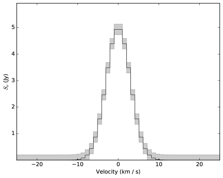
Figure 1: An example plotted spectrum showing the automated unit labeling and errors. The errors are shown with the ‘fill’ style and represent symmetric $1-\sigma$ Gaussian errors.

2.6.1 Automatic Error Estimation

In the case where there are portions of the spectrum that have no signal peaks, a common approach in spectroscopy is to estimate the errors from the standard deviation of those signal-free pixels. This approach assumes the noise is constant across the spectrum.

If all of the peaks present in the spectrum are fitted well by the model, the standard deviation of the residual spectrum from the model fit will accurately represent the uniform errors. If a fit is performed with uninitialized errors, they will initially default to a constant value of unity. pyspeckit will then automatically replace the errors with the standard deviation of the residuals, so they remain constant but will have a value that is related to the data. This means that performing a fit on the same data (without associated errors) twice will result in the same parameter values both times but different errors the second time.

2.6.2 Parameter error estimation

Parameter errors are adopted from the mpfit or lmfit fit results. The Levenberg-Marquardt algorithm finds a local minimum in parameter space, and one of its returns is the parameter covariance matrix. This covariance matrix is not directly the covariance of the parameters, and must be rescaled to deliver an approximate error.

The standard rescaling is to multiply the covariance by the sum of the squared errors divided by the degree of freedom of the fit, usually referred to as $\chi^{2}/N$. The number of degrees of freedom is assumed to be equal to the number of free parameters, e.g., for a one-dimensional Gaussian, there would be three: the amplitude, width, and center. This approach implicitly assumes that the model describes the data well and is an optimal fit. It also assumes that the model is linear with all of the parameters, at least in the region immediately surrounding the optimal fit. These requirements are frequently not satisfied; see Andrae et al. (2010) and Andrae (2010) for details. We show a demonstration of this approximation process in Appendix A for the case of a simple Gaussian line profile.

3 Graphical Design

3.1 GUI development

Many astronomers are familiar with IRAF’s splot tool, which is useful for fitting Gaussian profiles to spectral lines. It uses keyboard interaction to specify the fitting region and guesses for fitting the line profile, but for most use cases, these parameters could only be accessed through the GUI.

The fitting GUI in pyspeckit was built to match splot’s functionality but with additional means of interacting with the fitter. In splot, reproducing any given fit is challenging, since subtle changes in the cursor position (i.e., the input guess) can significantly change the fit result. In pyspeckit, it is possible to record the results of fits programmatically and re-fit using those same results.

The GUI was built using matplotlib’s canvas interaction tools. These tools are limited to the GUI capabilities that are compatible with all platforms (e.g., Qt, Tk, Gtk) and therefore exclude some of the more sophisticated fitting tools found in other software (e.g., glue; Beaumont et al., 2014).

An example walking through typical interactive GUI usage is in the online documentation at https://pyspeckit.readthedocs.io/en/latest/interactive.html.

3.2 Plotting

Plotting in pyspeckit is designed to provide a short path to publication-quality figures. The default plotting mode uses histogram-style line plots and labels axes with LaTeX-formatted versions of units.

When the plotter is active and a model is fit, the model parameters are displayed with LaTeX formatting in the plot legend. The errors on the parameters, if available, are also shown, and these uncertainties are used to decide on the number of significant figures to display.

4 Models

Some of pyspeckit’s internal functions may be replaced by the astropy  specutils package in the future. However, the rich suite modeling in pyspeckit is likely to remain useful indefinitely. This model library includes some of the most useful general spectral model functions (e.g., Gaussian, Lorentzian, and Voigt profiles) and a wide range of specific model types (e.g., ammonia and formaldehyde hyperfine models, the $\mathrm{H}_{2}$ rotational ladder, and recombination line models). These models can be easily used within pyspeckit, but they can also be used completely independent from it (e.g., https://nestfit.readthedocs.io/en/latest/quickstart.html, Svoboda 2021). Several of the models rely on scipy (Virtanen et al., 2020) for either special functions or multidimensional interpolation.

The base Model class and fitting framework in pyspeckit provide some generally useful features that do not need to be re-implemented. Any model is generalized to a multi-component form automatically; e.g., the Gaussian model only describes a single Gaussian spectral component, but the fitting tools allow any number of independent Gaussians to be fit.

Models are customizable, and examples of registering a new or modified model in pyspeckit are included in the online documentation.

A list of the included models, and their parent class when relevant, is given in Table 1

Table 1: Summary of Models

Model	Module Name	Parent class
Hyperfine	hyperfine	$\cdots$
Gaussian	inherited_gaussfitter	$\cdots$
Lorentzian	inherited_lorentzian	$\cdots$
Voigt	inherited_voigtfitter	$\cdots$
NH3	ammonia	Hyperfine
NH2D	ammonia	Hyperfine
N2H+	n2hp	Hyperfine
N2D+	n2dp	Hyperfine
DCO+	dcop	Hyperfine
LTE Molecule	lte_molecule	$\cdots$
H2CO (cm)	formaldehyde	Hyperfine
H2CO (mm)	formaldehyde_mm	$\cdots$
Hydrogen	hydrogen	$\cdots$

Hyperfine Line Models

In radio and millimeter spectroscopy, there are many molecular line groups that are well modelled as Gaussian profiles separated by fixed frequency offsets. These hyperfine line groups are often unique probes of physical parameters because these features have different, known relative optical depths. In this case, the measured relative amplitudes of these different features allow the optical depth (and, in turn, the column density) to be measured from a single spectrum. pyspeckit provides the hyperfine model class to handle this class of molecular line transitions, and it includes several molecular species implementations (e.g., HCN, N₂H⁺, NH₃, H₂CO). In this implementation, the excitation temperature of each of the hyperfine components is assumed to be the same, which is the most commonly used assumption but may be violated in some cases.

5 Cubes

Spectral cubes have become important in radio astronomy, since they are the natural data products produced by interferometers like ALMA and the JVLA. Optical and infrared data cubes are growing more common from integral field units (IFUs) like MUSE on the VLT, OSIRIS on Keck, NIFS on Gemini, and NIRSpec and MIRI on JWST.

The cube visualization tools built into pyspeckit are limited to spectral and spatial plots. The mapplot viewer makes a 2D image of a slice of the cube, if given a slice number, or a projection along the spectral axis if given a function or function name. Once active, the mapplot viewer can be used interactively: clicking on a pixel will display that pixel’s spectrum in a separate window; clicking and dragging will produce a circular region whose average spectrum will be plotted in that window. The plots shown in the separate window correspond to a spectrum accessible as the cube’s .spectrum object. This basic interaction allows for data exploration, but is not efficient for fitting each spectrum of a cube.

While many cube operations are handled well by numpy-based packages like spectral-cube (Robitaille et al., 2016; Ginsburg et al., 2019), it is sometimes desirable to fit a profile to each spectrum in a cube. The Cube.fiteach method is a tool for automated line fitting that includes parallelization of the fit. Examples can be found in the online documentation. This tool has seen significant use in custom made survey pipelines, where the library of spectral models is particularly useful (e.g, Friesen et al., 2017, https://github.com/GBTAmmoniaSurvey/GAS). It has also been incorporated into other tools, e.g., multicube, SCOUSE (Henshaw et al., 2016, 2019, see Appendix E), make_cube (Youngblood et al., 2016), and pyspecnest (Sokolov et al., 2020).

6 Summary

pyspeckit is a versatile tool for spectroscopic analysis in python and is one of the astropy affiliated packages.

Appendix A Parameter Error Estimation for a simple 1D Gaussian profile

As discussed in Section 2.6.2, parameter errors are estimated in pyspeckit by the underlying lmfit or mpfit tools using the approximation that the reduced chi-squared is unity, $\chi^{2}/n=1$. We demonstrate here that, for a simple one-dimensional Gaussian profile, this approximation results in an excellent recovery of the underlying parameter errors.

In Figure 2, we show a synthetic spectrum with uniform Gaussian random noise and perfectly-measured uncorrelated data errors. The fitted model is a one-dimensional Gaussian profile with free parameters amplitude, center, and width. The fit results are given in the figure.

To produce a good error estimate under the $\chi^{2}/n=1$ approximation, the error distribution must be Gaussian, the model must be linear in all parameters, and the model must be the correct underlying model (Andrae, 2010).

Figure 3 shows the $\chi^{2}$ values in parameter space surrounding the best-fit value. Along the diagonal, we show the $\chi^{2}$ values for the individual parameters with all others marginalized over by taking the minimum $\chi^{2}$ value over the explored parameter space. The vertical dashed lines show the estimated $1\sigma$ errors reported by the mpfit optimizer, while the horizontal dashed lines show the value $\Delta\chi^{2}=1$, which corresponds to the 68% confidence interval for that parameter. If the $\chi^{2}/n=1$ approximation is perfect, the dashed lines should intersect with the blue curves, and in this case, they do for all parameters.

Off of the diagonal of Figure 3, we show the two-dimensional marginal distributions. Contours are shown at $\Delta\chi^{2}=1,2.3,6.2,11.8$, corresponding to 39.3%, 68%, 95%, and 99.5% confidence regions (the first value corresponds to $1\sigma$ uncertainty when marginalized to a single parameter, while the others correspond to $1\sigma$, $2\sigma$, and $3\sigma$ for two parameters, respectively, assuming a normal distribution) . The vertical and horizontal dashed lines show the estimates from the $\chi^{2}/n=1$ approximation for a single parameter; these are expected to intersect the innermost 1$\sigma$ contour when marginalized to a single parameter. The shift vs amplitude and shift vs width diagrams are both well-behaved, with error contours tracing out a symmetric distribution centered on the true parameters marked with an ‘x’. However, the width vs amplitude plot indicates that the single-parameter errorbars are partly driven by the significantly correlated uncertainty between these parameters. This information is captured in the covariance matrix that is used to compute the single-parameter errors, as it has significant values in the off-diagonal parts of the matrix.

The source code for this example can be found in the pyspeckit github repository in examples/synthetic_spectrum_example_witherrorestimates.py.

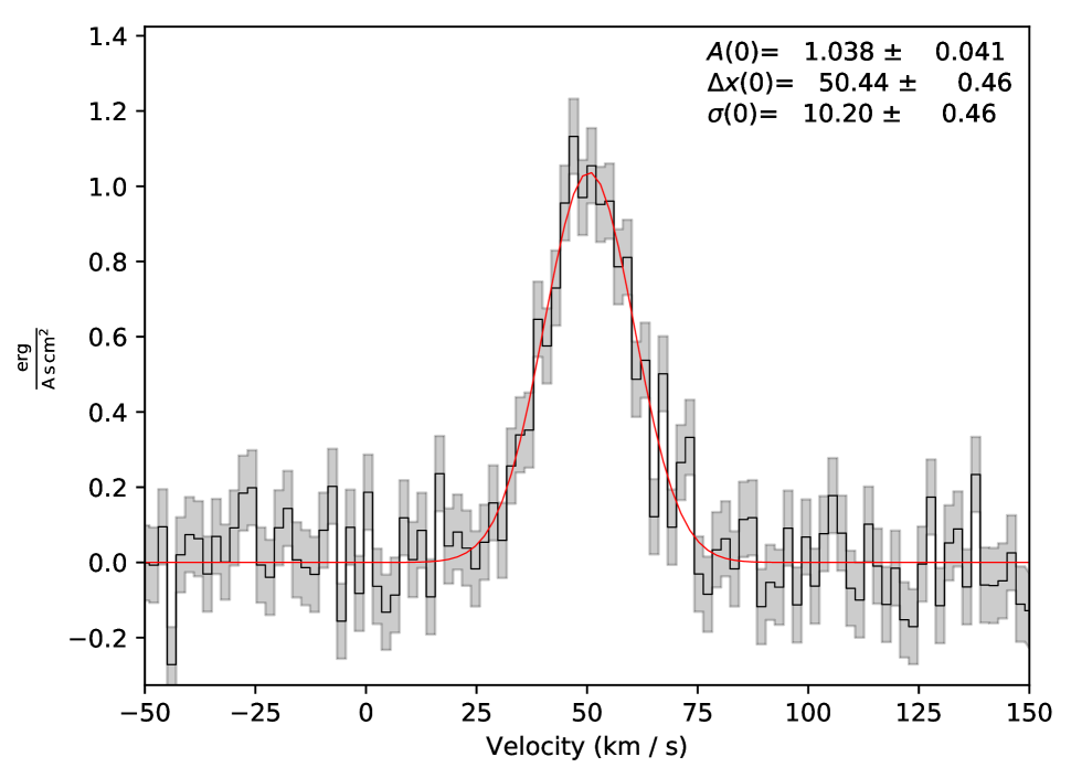
Figure 2: One-dimensional Gaussian profile fit to a synthetic spectrum. The parameter values and errors are shown in the upper right. The number of significant figures displayed in both the value and the error is automatically set to one digit more than the last significant digit in the error.

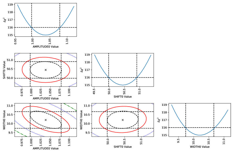
Figure 3: Error estimate figure. In all panels, the vertical dashed lines show the estimated $1\sigma$ errors from the optimizer, while the horizontal dashed lines show the value $\Delta\chi^{2}=1$, which corresponds to the 68% confidence interval for that parameter. In the off-diagonal panels, contours are shown at $\Delta\chi^{2}=1,2.3,6.2,11.8$ (black dashed, red, blue dotted, green dash-dot), corresponding to 39.3%, 68%, 95%, and 99.5% confidence regions ($1\sigma$ for a single parameter, then $1\sigma$, $2\sigma$, and $3\sigma$ for two parameters). See Appendix A for details and interpretation.

Appendix B Parameter Error Estimation for Ammonia

In Appendix A, we showed the parameter estimation results in the case of a modeled 1-dimensional Gaussian. One of the most commonly used models in pyspeckit is the ammonia ($\mathrm{NH}_{3}$) hyperfine model, which has several additional emission lines and several parameters governing those lines.

The ammonia inversion transitions are notable for having spectrally resolved hyperfine components under typical Galactic molecular gas conditions, the relative weights of which are governed by quantum mechanics (Mangum & Shirley, 2015). The existence of these additional components often allows for direct estimates of the optical depth of the central line, which is optically thicker than the other components, thereby making column density estimates from a single spectral band relatively straightforward.

The model for these lines is more complicated than that for a single Gaussian. The model must include a simplified version of the radiative transfer equation and must simultaneously produce the predicted emission of several lines. Additionally, there are several approximations for the relative line strengths that are convenient to use under different circumstances, so pyspeckit implements several different variants of the $\mathrm{NH}_{3}$ model.

In this section, we show parameter estimates analogous to those in Section A. We examine a case where the fitted lines are in local thermodynamic equilibrium (LTE), such that the ratios of the $(J,K)=(1,1)$ to $(2,2)$ line is governed by the rotational temperature $T_{\mathrm{R}}$ but the individual lines both have $T_{\mathrm{ex}}=T_{\mathrm{R}}$.

The free parameters in the ammonia model are the rotational temperature, $T_{\mathrm{R}}$, which governs the relative populations of the rotational states, the excitation temperature $T_{\mathrm{ex}}$, which governs the relative populations of the two levels within a single inversion transition, the column density, $N(\mathrm{NH}_{3})$, which specifies the total column density of $\mathrm{NH}_{3}$ integrated over all states (note that this parameter enters the model as $10^{N}$, i.e., we optimize the log of the column density), the line-of-sight velocity $v_{\mathrm{LoS}}$, the line width $\sigma_{v}$, and the ortho-to-para ratio parameterized as the fraction of ortho-$\mathrm{NH}_{3}$ $F_{ortho}$. In the examples below, we fix $F_{ortho}=0$ and treat only para-$\mathrm{NH}_{3}$ lines.

The fit results from the first case are shown in Figures 4 and 5. The fit recovers the input parameters, but reveals one of the important caveats when using any optimization algorithm: in some models, parameters are degenerate, and therefore using the diagonal of the covariance matrix to estimate the variance can result in incorrect error estimates. While the errors on most parameters appear reasonable, there is a very large error on the excitation temperature $T_{\mathrm{ex}}$, which is driven by the degeneracy of $T_{\mathrm{ex}}$ with $N_{\mathrm{tot}}$. The asymmetry of the error on $T_{\mathrm{ex}}$ is apparent in Figure 5, but it is not captured by the optimizer’s reported error results; the asymmetry occurs because $T_{ex}$ is in the exponent in the model equations.

In such situations, it can be beneficial to measure the parameter errors in different ways. Using the emcee and pymc wrappers can help do this. Examples of how to use these Monte Carlo samplers to acquire better parameter errors once an optimization has already been performed are available in the online documentation: see http://pyspeckit.readthedocs.io/en/latest/example_pymc.html.

More sophisticated examples, including fitting of a non-LTE ammonia spectrum in which $T_{\mathrm{ex}}<T_{R}$, are available in the example directory of pyspeckit (https://github.com/pyspeckit/pyspeckit/tree/master/examples), specifically https://github.com/pyspeckit/pyspeckit/tree/master/examples/synthetic_LTE_ammonia_spectrum_example_witherrorestimates.py and https://github.com/pyspeckit/pyspeckit/tree/master/examples/synthetic_nLTE_ammonia_spectrum_example_witherrorestimates.py.

These examples also include demonstrations of how to force the optimizer to ignore nonphysical values while still obtaining useful constraints on the free parameters. Constrained fitting approaches can be helpful in cases like the ammonia fit, where high values of $T_{ex}$ where $T_{ex}>T_{rot}$ are statistically likely given the model, but physically disallowed; constrained fitting allows the known physical limits to rule out bad portions of parameter space.

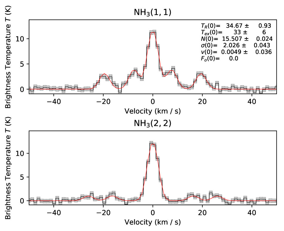
Figure 4: Ammonia model profile fit to a synthetic spectrum. The parameter values and errors are shown in the upper right. The associated error estimate triangle diagram is shown in Figure 5. The correct parameters are $T_{\mathrm{R}}=T_{\mathrm{ex}}=35$, $N=15$, $\sigma_{v}=2$, and $v=0$, all of which are reasonably recovered. However, note that $T_{\mathrm{ex}}>T_{\mathrm{R}}$ is generally nonphysical, yet the allowed parameter space for $T_{\mathrm{ex}}$ includes such values. This two-panel plot was produced automatically using the pyspeckit.wrappers.fitnh3.plot_nh3 command.

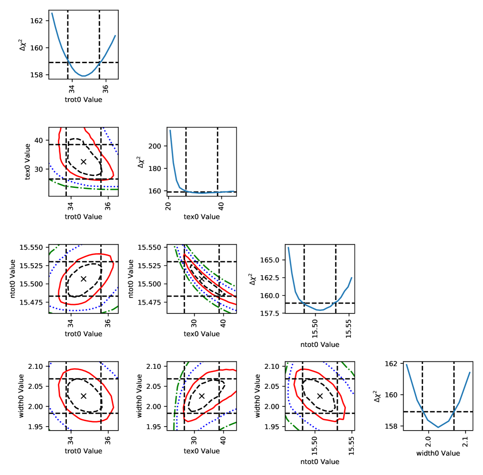
Figure 5: Error estimate figure for the default $\mathrm{NH}_{3}$ model. The panels are labeled as in Figure 3. The centroid velocity panel is excluded from this plot because it is independent of the other parameters, exhibiting no degeneracy. The most relevant panel is the ntot0 vs tex0 panel, which plots the column $N$ against the excitation temperature $T_{\mathrm{ex}}$: both of these parameters govern the peak amplitude of the spectrum, so they are degenerate. The vertical and horizontal dashed lines represent the $\delta\chi^{2}=1$ and $\pm 1\sigma$ computed errors, respectively. Their intersection points also intersect the blue marginalized $\delta\chi^{2}$ curve in all of the displayed cases, indicating that the approximation of the errors using the $\chi^{2}/n=1$ assumption is excellent. However, the asymmetry seen in the blue $T_{ex}$ curve suggests that the approximation for that parameter is likely to break down in some cases because the true errors are asymmetric.

Appendix C Comparison of N₂H⁺ (1-0) results with CLASS

One of the most frequently used line transitions for the study of dense gas kinematics is N₂H⁺ (1-0) at 93.17 GHz. The transition displays several hyperfine components with well determined relative frequencies and weights. The standard approach for analyzing this line has been to use the HFS mode within CLASS. Here we show that using the N₂H⁺ hyperfine model in pyspeckit, we obtain the same results in both optically thin and thick models.

The main difference between the CLASS and pyspeckit parametrization is that the former does not report excitation temperature ($T_{ex}$), but the area of the line profile. The reported area is $\tau\times T_{ant}$, where

$$T_{ant}=J(T_{ex})-J(T_{background})~{},$$ (C1)

where

$$J_{\nu}(T)=\frac{h\,\nu}{k_{B}}\frac{1}{(e^{h\,\nu/k_{B}\,T}-1)}~{}.$$ (C2)

We derive the equivalent $T_{ex}$ from the reported line fit parameters. Moreover, in the optically thin case both fits are performed using the common assumption of $\tau=0.1$ as a fixed parameter.

Tables 2 and 3 show the results of fitting an example spectrum in both CLASS and pyspeckit. The resulting fits differ by $<1\%$ in most parameters, with a slightly greater discrepancy in the velocity centroid but consistent within the reported fit uncertainties.

Table 2: Best fit parameters in optically thin model (3 parameters)

Parameter	Input value	pyspeckit fit	CLASS fit
Tex	9.0	3.454$\pm$0.014	3.451
$V_{c}$	0.0	0.0016	0.0028$\pm$0.0068
$\sigma_{v}$	0.3	0.2942$\pm$0.0062	0.2930$\pm$0.0060
$\tau_{all}$	0.01	0.1	0.1
$Area$			0.0607$\pm$0.0012

Table 3: Best fit parameters in optically thick model (4 parameters)

Parameter	Input value	pyspeckit fit	CLASS fit
Tex	9.0	9.19$\pm$0.19	9.1833
$V_{c}$	0.0	0.00042	-0.000$\pm$0.0063
$\sigma_{v}$	0.3	0.3047$\pm$0.0062	0.3041$\pm$0.0063
$\tau_{all}$	9.0	8.13$\pm$0.59	8.10$\pm$0.59
$Area$			49.0$\pm$2.25

Appendix D LTE Model

pyspeckit includes tools to model generic local thermodynamic equilibrium (LTE) emission lines. The modeling tools include wrappers to retrieve the appropriate molecular line parameters from the JPL (Pickett et al., 1998) or CDMS (Müller et al., 2005) spectroscopy databases via their astroquery interfaces (Ginsburg et al., 2019).

The main modeling function, LTE_molecule.generate_model, operates on the combination of line parameters (centroid, width), physical parameters (excitation temperature $T_{ex}$, total column density $N_{tot}$), and molecular line parameters (rest frequency $\nu_{rest}$, Einstein A value $A_{ij}$, degeneracy $g_{u}$, upper state energy level $E_{U}$, and the partition function $Q(T_{ex})$). It implements the equations:

$$\tau_{\nu}=\frac{c^{2}}{8\pi\nu^{2}}A_{ij}N_{u}\phi_{\nu}\left[\exp\left(\frac{h\nu}{k_{B}T_{ex}}\right)-1\right]$$ (D1)

where $c$ is the speed of light, $k_{B}$ is Boltzmann’s constant, $h$ is Planck’s constant, $N_{u}$ is given by

$$N_{u}=N_{tot}\frac{g_{u}}{Q}\exp\left(\frac{-E_{u}}{k_{B}T_{ex}}\right)$$ (D2)

and $\phi_{\nu}$ is assumed to be a Gaussian such that

$$\phi_{\nu}=\frac{1}{\sqrt{2\pi}\sigma_{\nu}}\exp\left[-\frac{(\nu-\nu_{0})^{2}}{2\sigma_{\nu}^{2}}\right]$$ (D3)

where $\sigma_{\nu}$ is the Gaussian line width (not the FWHM) in frequency units, $\sigma_{\nu}=\frac{\sigma_{v}}{c}\nu_{rest}$ and $\sigma_{v}$ is the Gaussian line width in velocity units. The above is based on Equations 11 and 29 of Mangum & Shirley (2015). The returned spectral model is then calculated as

$$\begin{array}[]{lll}I_{\nu}&=&J_{\nu}(T_{ex})\left[1-e^{-\tau}\right]+J_{\nu}(T_{BG})e^{-\tau}-J_{\nu}(T_{BG})\\ &=&\left[J_{\nu}(T_{ex})-J_{\nu}(T_{BG})\right]\left[1-e^{-\tau}\right]\\ \end{array}$$ (D4)

where $T_{BG}$ is the background temperature (assumed 2.73 for the default CMB temperature). We have split the equation into two lines to indicate that the return is explicitly background-subtracted. $J_{\nu}$ is the Rayleigh-Jeans equivalent brightness temperature

$$J_{\nu}=\frac{h\nu}{k_{B}}\left[\exp\left(\frac{-h\nu}{k_{B}T}\right)-1\right]^{-1}$$ (D5)

. The partition function can be specified as an array, which enables modeling lines from different species simultaneously.

To verify the accuracy of these models, we benchmarked the pyspeckit models against both XCLASS (Möller et al., 2017) and molsim (Lee, 2021). The benchmark notebook is provided here: https://github.com/pyspeckit/pyspeckit-tests/blob/master/xclass-benchmark/CO_Benchmark.ipynb. We modeled the lowest 12 transitions of CO. We obtain good agreement ($<1\%$ difference) with XCLASS at the line peak for all transitions when using option Interf_Flag = False. In the low-J transitions, we see significant fractional differences in the line wings, but with very small absolute values (the difference in the integral is $<10^{-4}$); these appear to come from rounding errors in the evaluation of the Gaussian function. These small differences are very unlikely to affect any modeling. We obtain significantly different answers with Interf_Flag = True; in this case, XCLASS returns a peak that is lower by the CMB temperature.

We additionally benchmarked two more complicated molecules, CH₃OH and CH₃CN, and again found excellent agreement.

Appendix E ScousePy

ScousePy is a tool for the decomposition of data cubes with multi-component spectral lines, and makes use of pyspeckit’s fitting functionality (§2.3). Broadly speaking, spectral decomposition algorithms can be divided into two classes: bottom-up and top-down. The former treat the decomposition of individual spectra independently from one another, while the latter approach uses spatial averaging to estimate initial guesses for the decomposition of individual spectra. ScousePy follows the latter of these two approaches. ScousePy

1. breaks a data cube into sub-regions of user-defined size. A spatially averaged spectrum is extracted from each sub-region.

2. uses derivative spectroscopy to estimate the number of components and the properties of those individual components in each spatially-averaged spectrum. These initial guesses are passed to pyspeckit’s specfit to perform the fit.

3. uses the output solution (specfit.fitter.params) from the average spectrum as new initial guesses for fitting the individual spectra contained within the averaging region.

4. displays the results in an interface that enables quality assessment and re-fitting if necessary.

ScousePy makes use of pyspeckit’s specfit in two main ways. First, non-interactively, with initial guesses supplied to specfit via specfit.guesses. Second, ScousePy also makes use of pyspeckit’s interactive fitting functionality, which uses keyboard and mouse interaction to provide specfit.guesses.

An example of the ScousePy.ScouseFitter GUI is shown in Figure 6. This figure shows the Gaussian decomposition of a two component spectrum. ScousePy provides initial guesses to pyspeckit’s specfit using derivative spectroscopy, in which:

1. the input spectrum is smoothed using astropy.convolution.Gaussian1DKernel (see ScousePy.DSpec).

2. the first to fourth order derivatives of the smoothed spectrum are computed and used to determine the number of components and their amplitudes, centroids, and widths (see lollipops in the top left panel).

These values are then supplied to specfit via specfit.guesses. The fit is performed using lmfit, and the result is displayed in the information panel. The buttons on the right hand side of the GUI can be used to enter pyspeckit’s interactive fitter functionality via “fit (manual)” . The relevant fit information produced by pyspeckit (or further derived from the quantities output by specfit) are located in a dictionary called ScousePy.ScouseFitter.modelstore. Further information on the pyspeckit methodology used by ScousePy can be found in the documentation for ScousePy.ScouseFitter and ScousePy.Decomposer (see https://scousepy.readthedocs.io/en/latest/).

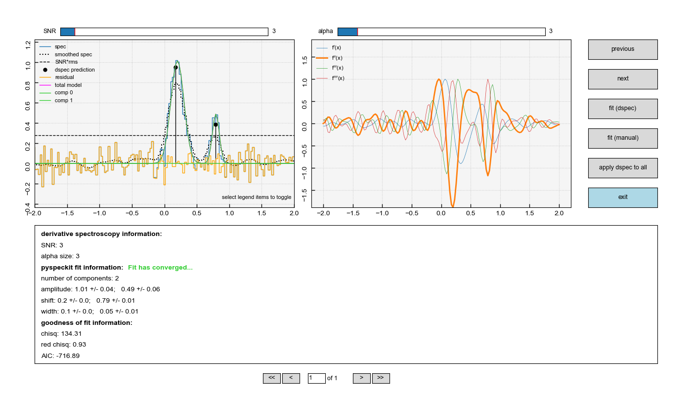
Figure 6: Gaussian decomposition of a two-component spectrum performed by ScousePy using pyspeckit. The top-left panel shows the spectrum (black), the same spectrum smoothed with a Gaussian 1D kernel (dotted black line) using astropy.convolution.Gaussian1DKernel, which is used for the derivative spectroscopy (right panel), the location and amplitude of the initial guesses determined from derivative spectroscopy (black lollipops) and supplied to specfit, the best fitting model solution (green and magenta lines indicate individual components and the total model), the residual spectrum after subtracting the model (orange line), and the $3\sigma$ noise level determined from ScousePy.getnoise. The top-right panel shows the first to fourth derivatives of the smoothed spectrum (dotted black line). These derivatives are used to estimate the number of components and their amplitudes, widths, and centroids (ScousePy.DSpec). The information panel at the bottom shows the output information from pyspeckit. This information includes the model parameters and their uncertainties and goodness-of-fit statistics. The buttons on the right can be used to control pyspeckit either non-interactively using “fit (dspec)” or interactively using “fit (manual)”.

References

- Andrae (2010) Andrae, R. 2010, arXiv e-prints, arXiv:1009.2755. https://arxiv.org/abs/1009.2755
- Andrae et al. (2010) Andrae, R., Schulze-Hartung, T., & Melchior, P. 2010, arXiv e-prints, arXiv:1012.3754. https://arxiv.org/abs/1012.3754
- Astropy Collaboration et al. (2013) Astropy Collaboration, Robitaille, T. P., Tollerud, E. J., et al. 2013, A&A, 558, A33, doi: 10.1051/0004-6361/201322068
- Astropy Collaboration et al. (2018) Astropy Collaboration, Price-Whelan, A. M., Sipőcz, B. M., et al. 2018, AJ, 156, 123, doi: 10.3847/1538-3881/aabc4f
- Beaumont et al. (2014) Beaumont, C., Robitaille, T., & Borkin, M. 2014, Glue: Linked data visualizations across multiple files, Astrophysics Source Code Library, record ascl:1402.002. http://ascl.net/1402.002
- Foreman-Mackey et al. (2013) Foreman-Mackey, D., Hogg, D. W., Lang, D., & Goodman, J. 2013, PASP, 125, 306, doi: 10.1086/670067
- Friesen et al. (2017) Friesen, R. K., Pineda, J. E., co-PIs, et al. 2017, ApJ, 843, 63, doi: 10.3847/1538-4357/aa6d58
- Garwood (2000) Garwood, R. W. 2000, in Astronomical Society of the Pacific Conference Series, Vol. 216, Astronomical Data Analysis Software and Systems IX, ed. N. Manset, C. Veillet, & D. Crabtree, 243
- Gildas Team (2013) Gildas Team. 2013, GILDAS: Grenoble Image and Line Data Analysis Software, Astrophysics Source Code Library, record ascl:1305.010. http://ascl.net/1305.010
- Ginsburg et al. (2019) Ginsburg, A., Sipőcz, B. M., Brasseur, C. E., et al. 2019, AJ, 157, 98, doi: 10.3847/1538-3881/aafc33
- Ginsburg et al. (2022) Ginsburg, A., Mirocha, J., Sokolov, V., et al. 2022, pyspeckit/pyspeckit, v1.0.0, Zenodo, doi: 10.5281/zenodo.6470904. https://doi.org/10.5281/zenodo.6470904
- Greisen et al. (2006) Greisen, E. W., Calabretta, M. R., Valdes, F. G., & Allen, S. L. 2006, A&A, 446, 747, doi: 10.1051/0004-6361:20053818
- Harris et al. (2020) Harris, C. R., Millman, K. J., van der Walt, S. J., et al. 2020, Nature, 585, 357, doi: 10.1038/s41586-020-2649-2
- Harris et al. (2020) Harris, C. R., Millman, K. J., van der Walt, S. J., et al. 2020, Nature, 585, 357, doi: 10.1038/s41586-020-2649-2
- Henshaw et al. (2016) Henshaw, J. D., Longmore, S. N., Kruijssen, J. M. D., et al. 2016, MNRAS, 457, 2675, doi: 10.1093/mnras/stw121
- Henshaw et al. (2019) Henshaw, J. D., Ginsburg, A., Haworth, T. J., et al. 2019, MNRAS, 485, 2457, doi: 10.1093/mnras/stz471
- Lee (2021) Lee, K. 2021, bmcguir2/molsim: Updated contributor list, v0.1.2a, Zenodo, doi: 10.5281/zenodo.4560750
- Levenberg (1944) Levenberg, K. 1944, Quarterly of Applied Mathematics, 2, 164, doi: 10.1090/qam/10666
- Mangum & Shirley (2015) Mangum, J. G., & Shirley, Y. L. 2015, PASP, 127, 266, doi: 10.1086/680323
- Markwardt (2009) Markwardt, C. B. 2009, in Astronomical Society of the Pacific Conference Series, Vol. 411, Astronomical Data Analysis Software and Systems XVIII, ed. D. A. Bohlender, D. Durand, & P. Dowler, 251
- Marquardt (1963) Marquardt, D. W. 1963, Journal of the Society for Industrial and Applied Mathematics, 11, 431, doi: 10.1137/0111030
- Möller et al. (2017) Möller, T., Endres, C., & Schilke, P. 2017, A&A, 598, A7, doi: 10.1051/0004-6361/201527203
- Momcheva & Tollerud (2015) Momcheva, I., & Tollerud, E. 2015, ArXiv e-prints
- Müller et al. (2005) Müller, H. S. P., Schlöder, F., Stutzki, J., & Winnewisser, G. 2005, Journal of Molecular Structure, 742, 215, doi: 10.1016/j.molstruc.2005.01.027
- Newville et al. (2014) Newville, M., Stensitzki, T., Allen, D. B., & Ingargiola, A. 2014, LMFIT: Non-Linear Least-Square Minimization and Curve-Fitting for Python, 0.8.0, Zenodo, doi: 10.5281/zenodo.11813
- Pence et al. (2010) Pence, W. D., Chiappetti, L., Page, C. G., Shaw, R. A., & Stobie, E. 2010, A&A, 524, A42, doi: 10.1051/0004-6361/201015362
- Pickett et al. (1998) Pickett, H. M., Poynter, R. L., Cohen, E. A., et al. 1998, J. Quant. Spec. Radiat. Transf., 60, 883, doi: 10.1016/S0022-4073(98)00091-0
- Robitaille et al. (2016) Robitaille, T., Ginsburg, A., Beaumont, C., Leroy, A., & Rosolowsky, E. 2016, spectral-cube: Read and analyze astrophysical spectral data cubes, Astrophysics Source Code Library, record ascl:1609.017. http://ascl.net/1609.017
- Salvatier et al. (2016) Salvatier, J., Wieckiâ, T. V., & Fonnesbeck, C. 2016, PyMC3: Python probabilistic programming framework, doi: 10.7717/peerj-cs.55
- Sokolov et al. (2020) Sokolov, V., Pineda, J. E., Buchner, J., & Caselli, P. 2020, ApJ, 892, L32, doi: 10.3847/2041-8213/ab8018
- Svoboda (2021) Svoboda, B. 2021, autocorr/nestfit: Initial public release, v0.2, Zenodo, doi: 10.5281/zenodo.4470028. https://urldefense.proofpoint.com/v2/url?u=https-3A__doi.org_10.5281_zenodo.4470028&d=DwIGAg&c=sJ6xIWYx-zLMB3EPkvcnVg&r=Z1XKDJQAeQrijyDtjaW9Wgu01lnkYrUgUcy1mQEqN5M&m=GPa5YygYSU5myWqo_ooDDI-f16r16bIMGSpxN_pjT7_YqNng4UTOOsO-DTx27IQk&s=8m9VVLbHI3KlUkzDWW57LfumtvEXB1xWsXCYq_jZAs0&e=
- Tody (1986) Tody, D. 1986, in Society of Photo-Optical Instrumentation Engineers (SPIE) Conference Series, Vol. 627, Instrumentation in astronomy VI, ed. D. L. Crawford, 733
- Tollerud (2012) Tollerud, E. 2012, Astropysics: Astrophysics utilities for python, Astrophysics Source Code Library, record ascl:1207.007. http://ascl.net/1207.007
- van der Walt et al. (2011) van der Walt, S., Colbert, S. C., & Varoquaux, G. 2011, Computing in Science and Engineering, 13, 22, doi: 10.1109/MCSE.2011.37
- Virtanen et al. (2020) Virtanen, P., Gommers, R., Oliphant, T. E., et al. 2020, Nature Methods, 17, 261, doi: 10.1038/s41592-019-0686-2
- Wells et al. (1981) Wells, D. C., Greisen, E. W., & Harten, R. H. 1981, A&AS, 44, 363
- Youngblood et al. (2016) Youngblood, A., Ginsburg, A., & Bally, J. 2016, AJ, 151, 173, doi: 10.3847/0004-6256/151/6/173