The first 7 months of the 2020 X-ray outburst of the magnetar SGR J1935+2154
Abstract
The magnetar SGR J1935+2154 underwent a new active episode on 2020 April 27–28, when a forest of hundreds of X-ray bursts and a large enhancement of the persistent flux were detected. For the first time, a radio burst with properties similar to those of fast radio bursts and with a X-ray counterpart was observed from this source, showing that magnetars can power at least a group of fast radio bursts. In this paper, we report on the X-ray spectral and timing properties of SGR J1935+2154 based on a long-term monitoring campaign with Chandra, XMM–Newton, NuSTAR, Swift and NICER covering a time span of months since the outburst onset. The broadband spectrum exhibited a non-thermal power-law component () extending up to keV throughout the campaign and a blackbody component with temperature decreasing from keV at the outburst peak to keV in the following months. We found that the luminosity decay is well described by the sum of two exponential functions, reflecting the fast decay (1 d) at the early stage of the outburst followed by a slower decrease (30 d). The source reached quiescence about days after the outburst onset, releasing an energy of erg during the outburst. We detected X-ray pulsations in the XMM–Newton data sets and derived an average spin-down rate of s s-1 using the spin period measurements derived in this work and three values reported previously during the same active period. Moreover, we report on simultaneous radio observations performed with the Sardinia Radio Telescope. No evidence for periodic or single-pulse radio emission was found.
keywords:
Magnetars; Neutron stars; Radio pulsars; Transient sources; X-ray bursts1 Introduction
Among isolated neutron stars, magnetars are the most active, with a distinctive high-energy phenomenology (see, e.g., Kaspi & Beloborodov, 2017; Esposito et al., 2021, for recent reviews). Powered by their own magnetic energy, which is stored in a superstrong field (up to 1015 G at the surface), these objects emit X-ray/gamma-ray bursts that last from milliseconds to tens of minutes and reach a wide range of X-ray peak luminosities, 1039 – 1045 erg s-1. These flaring events are often accompanied by long-lived (up to years) enhancements of the persistent X-ray luminosity, the so-called outbursts (see http://magnetars.ice.csic.es; Coti Zelati et al., 2018).
Discovered in 2014 (Stamatikos et al., 2014), SGR J1935+2154 (henceforth SGR J1935) has a spin period s and a spin-down rate s s-1, implying a surface dipolar magnetic field G at the pole (Israel et al., 2016). Since its discovery, SGR J1935 has been one of the most active magnetars, showing outbursts in 2015 February, 2016 May and June, and frequent bursting episodes (see, e.g., Younes et al., 2017; Lin et al., 2020b). Its latest reactivation dates back to 2020 April 27, when several X-ray and gamma-ray instruments detected a burst storm and an increase of the persistent X-ray flux (e.g., Palmer, 2020; Younes et al., 2020). A day after the initial trigger, the Canadian Hydrogen Intensity Mapping Experiment (CHIME) and the Survey for Transient Astronomical Radio Emission 2 (STARE2) independently detected an extremely bright radio burst (Andersen et al., 2020; Bochenek et al., 2020), with morphology reminiscent of that of Fast Radio Bursts (FRBs; see, e.g., Caleb & Keane, 2021, for a review). The energy released was about three orders of magnitude larger than that of any radio pulse from the Crab pulsar (the source emitting the brightest Galactic radio pulses; Bera & Chengalur 2019) and any giant pulse detected from the radio magnetar XTE J1810–197 (Caleb et al., 2022), and 50 times smaller than that released by the weakest extragalactic FRB observed so far (e.g., Marcote et al., 2020). This detection strengthened the hypothesis that at least a sub-group of FRBs can be powered by magnetars at cosmological distances (Beloborodov, 2017; Margalit et al., 2020). Moreover, the radio burst was temporally coincident with a hard X-ray burst (Mereghetti et al., 2020; Tavani et al., 2021; Ridnaia et al., 2021), showing for the first time that magnetar bursts can have a bright radio counterpart. Furthermore, analysis of simultaneous radio and X-ray archival observations of magnetars revealed two FRB-like bursts from another source, 1E 1547.0–5408 (Israel et al., 2021). One of the radio bursts was anticipated by 1 s by a short X-ray burst, resulting in a radio-to-X-ray fluence ratio of 10-9, proving that magnetars can emit radio bursts with fluences spanning over a wide range.
No pulsed radio emission from SGR J1935 was detected in the immediate aftermath of the FRB-like event (Lin et al., 2020a). Coordinated radio and X-ray monitoring campaigns were initiated. While no other simultaneous radio and X-ray bursts were observed, SGR J1935 emitted a few more fainter radio bursts (Kirsten et al., 2020; Zhang et al., 2020) and several X-ray short bursts (see http://enghxmt.ihep.ac.cn/bfy/331.jhtml and Table 2 by Borghese et al. 2020). On 2020 October 8, CHIME detected three additional radio bursts from the direction of SGR J1935, all clustered within one rotational period cycle (Good & Chime/Frb Collaboration, 2020). Follow-up observations with the Five-hundred-metre Aperture Sperical Telescope (FAST) caught numerous single pulses from the source and also detected pulsed radio emission (Zhu et al., 2020). These detections indicated that SGR J1935 can emit radio bursts with energies spanning nearly seven orders of magnitude and switch on/off in the radio band.
Here, we report on the results of the X-ray long-term monitoring campaign of SGR J1935 covering the first 7 months of the outburst decay since its reactivation on 2020 April 27. We first summarise the data analysis procedure in Section 2. We then present the timing and spectral analysis, as well as a search for short bursts in Section 3. Simultaneous radio observations are described in Section 4. Finally, we discuss our findings in Section 5.
| X-ray Instrumenta | Obs.ID | Start | Stop | Exposure | Count Rateb | Fluxc | ||
|---|---|---|---|---|---|---|---|---|
| YYYY-MM-DD hh:mm:ss (TT) | (ks) | (counts s-1) | (keV) | (km) | (10-12 cgs) | |||
| Chandra/ACIS (TE) | 22431 | 2020-04-30 20:30:28 | 2020-05-01 02:44:51 | 19.8 | 0.1470.003 | 0.510.03 | 2.10.2 | 4.60.4 |
| Chandra/ACIS (TE) | 22432 | 2020-05-02 08:58:14 | 2020-05-02 23:29:51 | 49.9 | 0.1370.002 | 0.560.01 | 1.340.05 | 4.00.1 |
| XMM–Newton/EPIC-pn (FF) | 0871190201 | 2020-05-13 21:43:24 | 2020-05-14 10:54:26 | 28.3 | 0.3880.004 | 0.450.01 | 1.70.1 | 2.50.1 |
| Chandra/ACIS (TE) | 23251 | 2020-05-18 10:48:14 | 2020-05-18 16:32:19 | 18.8 | 0.1160.002 | 0.500.01 | 1.50.1 | 3.00.1 |
| NICER/XTI | 3655010201 | 2020-05-18 05:36:06 | 2020-05-18 13:38:40 | 4.7 | 0.290.01 | 0.490.02 | 1.30.2 | 0.90.1 |
| NICER/XTI | 3020560105d1 | 2020-05-19 21:53:47 | 2020-05-19 22:10:40 | 0.9 | 0.500.03 | 0.51 | 1.50.2 | 1.70.1 |
| NICER/XTI | 3020560106d1 | 2020-05-20 07:39:40 | 2020-05-20 15:37:20 | 0.6 | 0.670.04 | 0.51 | 1.50.2 | 1.70.1 |
| NICER/XTI | 3020560107 | 2020-05-22 00:59:19 | 2020-05-22 22:54:46 | 5.1 | 0.490.01 | 0.470.02 | 1.50.1 | 2.10.1 |
| NICER/XTI | 3020560108 | 2020-05-23 00:13:19 | 2020-05-23 09:42:50 | 3.2 | 0.390.02 | 0.450.02 | 1.80.2 | 1.00.1 |
| NICER/XTI | 3020560109d2 | 2020-05-25 14:13:00 | 2020-05-25 15:55:32 | 0.8 | 0.530.03 | 0.440.02 | 1.80.1 | 1.80.1 |
| Swift/XRT (PC) | 00033349067 | 2020-05-28 12:10:39 | 2020-05-28 16:59:54 | 2.0 | 0.0240.004 | 0.37 | 1.8 | 1.9 |
| NICER/XTI | 3020560110d2 | 2020-05-28 21:10:39 | 2020-05-28 23:00:55 | 1.7 | 0.430.02 | 0.440.02 | 1.80.1 | 1.80.1 |
| NICER/XTI | 3020560111d3 | 2020-05-29 03:22:38 | 2020-05-29 03:39:46 | 0.9 | 0.380.03 | 0.480.04 | 1.50.02 | 1.70.1 |
| NICER/XTI | 3020560112d3 | 2020-05-30 05:42:03 | 2020-05-30 18:18:57 | 1.3 | 0.490.03 | 0.480.04 | 1.50.02 | 1.70.1 |
| NICER/XTI | 3020560113d4 | 2020-05-31 01:50:42 | 2020-05-31 11:24:40 | 1.1 | 0.490.03 | 0.430.02 | 1.60.02 | 2.60.2 |
| NICER/XTI | 3020560114d4 | 2020-06-01 02:37:42 | 2020-06-01 21:50:40 | 2.7 | 0.430.02 | 0.430.02 | 1.60.02 | 2.60.2 |
| NICER/XTI | 3020560115d4 | 2020-06-02 23:34:38 | 2020-06-02 23:51:40 | 1.0 | 0.470.03 | 0.430.02 | 1.60.02 | 2.60.2 |
| NICER/XTI | 3020560116d5 | 2020-06-03 04:12:40 | 2020-06-03 04:25:13 | 0.7 | 0.410.04 | 0.500.02 | 1.20.1 | 0.90.1 |
| NICER/XTI | 3020560117d5 | 2020-06-04 12:45:40 | 2020-06-04 13:10:23 | 1.4 | 0.370.02 | 0.500.02 | 1.20.1 | 0.90.1 |
| Swift/XRT (PC) | 00033349068 | 2020-06-05 03:37:29 | 2020-06-05 09:53:53 | 1.5 | 0.0210.004 | 0.4 | 1.6 | 2.6 |
| NICER/XTI | 3020560118d5 | 2020-06-05 04:14:56 | 2020-06-05 16:59:23 | 1.2 | 0.300.02 | 0.500.02 | 1.20.1 | 0.90.1 |
| NICER/XTI | 3020560119d5 | 2020-06-06 05:03:57 | 2020-06-06T05:22:00 | 1.0 | 0.200.02 | 0.500.02 | 1.20.1 | 0.90.1 |
| Swift/XRT (PC) | 00033349069 | 2020-06-11 01:14:49 | 2020-06-11 14:16:52 | 2.5 | 0.0230.003 | 0.55 | 0.9 | 2.90.4 |
| NuSTAR FPMA/B | 80602313006e | 2020-06-14 06:46:09 | 2020-06-14 23:21:09 | 30.1/29.4 | 0.0730.002 | 0.440.04 | 2.00.1 | |
| Swift/XRT (PC) | 00089040001e | 2020-06-14 10:25:15 | 2020-06-1413:49:53 | 1.9 | 0.0290.004 | 0.440.04 | 2.00.1 | |
| NICER/XTI | 3655010301d6 | 2020-06-17 21:38:39 | 2020-06-17 22:06:40 | 1.2 | 0.330.03 | 0.460.01 | 1.40.1 | 1.40.1 |
| Swift/XRT (PC) | 00033349070 | 2020-06-18 08:23:18 | 2020-06-18 23:11:53 | 2.7 | 0.0290.003 | 0.50 | 1.4 | 1.40.2 |
| NICER/XTI | 3655010302d6 | 2020-06-18 08:29:43 | 2020-06-18 21:21:20 | 6.6 | 0.380.01 | 0.460.01 | 1.40.1 | 1.40.1 |
| NICER/XTI | 3655010303d6 | 2020-06-18 23:59:32 | 2020-06-19 09:45:00 | 4.1 | 0.210.01 | 0.460.01 | 1.40.1 | 1.40.1 |
| NICER/XTI | 3020560120d7 | 2020-06-20 21:05:40 | 2020-06-20 21:23:40 | 0.9 | 0.460.03 | 0.420.01 | 1.80.2 | 1.70.1 |
| NICER/XTI | 3020560121d7 | 2020-06-21 00:01:20 | 2020-06-21 00:29:20 | 0.8 | 0.310.03 | 0.420.01 | 1.80.2 | 1.70.1 |
| NICER/XTI | 3020560122d7 | 2020-06-22 10:17:00 | 2020-06-22 10:49:20 | 1.7 | 0.410.02 | 0.420.01 | 1.80.2 | 1.70.1 |
| NICER/XTI | 3020560123 | 2020-06-23 01:36:00 | 2020-06-23 17:48:20 | 3.2 | 0.310.01 | 0.450.01 | 1.50.1 | 0.80.1 |
| NICER/XTI | 3020560124d8 | 2020-06-24 22:41:19 | 2020-06-24 23:13:11 | 1.8 | 0.350.02 | 0.470.02 | 1.50.01 | 1.00.1 |
| Swift/XRT (PC) | 00033349071 | 2020-06-25 01:30:52 | 2020-06-25 17:43:52 | 3.2 | 0.0250.003 | 0.380.06 | 1.9 | 1.6 |
| NICER/XTI | 3020560125d8 | 2020-06-25 21:57:00 | 2020-06-25 22:29:00 | 1.6 | 0.370.03 | 0.470.02 | 1.50.01 | 1.00.1 |
-
a
The instrumental setup is indicated in brackets: TE = timed exposure, FF = full frame, PC = photon counting, WT = windowed timing.
-
b
Count rate, computed after removing bursts, in the 0.3–10 keV range for Swift and XMM–Newton, in the 0.3–8 keV interval for Chandra, in the 1–5 keV band for NICER, and in the 3–20 keV range for NuSTAR summing up the two FPMs. Uncertainties are at 1 c.l.
-
c
Observed 0.3–10 keV flux in units of 10-12 erg cm-2 s-1.
-
d,e,f
The spectra extracted from these observations were fitted jointly, tying up all model parameters (see Section 3.2.1 for details).
| X-ray Instrumenta | Obs.ID | Start | Stop | Exposure | Count Rateb | Fluxc | ||
|---|---|---|---|---|---|---|---|---|
| YYYY-MM-DD hh:mm:ss (TT) | (ks) | (counts s-1) | (keV) | (km) | (10-12 cgs) | |||
| NICER/XTI | 3020560126d9 | 2020-06-27 14:29:00 | 2020-06-27 14:45:20 | 0.8 | 0.380.03 | 0.450.03 | 1.50.2 | 1.10.1 |
| NICER/XTI | 3020560127d9 | 2020-06-28 16:31:00 | 2020-06-28 17:04:51 | 1.7 | 0.290.02 | 0.450.03 | 1.50.2 | 1.10.1 |
| NICER/XTI | 3020560128d9 | 2020-06-29 18:53:20 | 2020-06-29 19:24:40 | 1.7 | 0.310.02 | 0.450.03 | 1.50.2 | 1.10.1 |
| NICER/XTI | 3020560129d10 | 2020-06-30 16:19:20 | 2020-06-30 17:03:20 | 2.1 | 0.290.02 | 0.460.01 | 1.50.1 | 0.90.1 |
| NICER/XTI | 3020560130d10 | 2020-07-01 12:25:57 | 2020-07-01 12:40:50 | 0.6 | 0.410.04 | 0.460.01 | 1.50.1 | 0.90.1 |
| NICER/XTI | 3020560131d10 | 2020-07-02 11:41:29 | 2020-07-02 12:03:20 | 1.2 | 0.270.02 | 0.460.01 | 1.50.1 | 0.90.1 |
| Swift/XRT (PC) | 00033349072 | 2020-07-02 16:24:24 | 2020-07-02 18:27:52 | 3.2 | 0.0260.003 | 0.51 | 1.2 | 3.40.4 |
| NICER/XTI | 3020560132d10 | 2020-07-03 14:01:00 | 2020-07-03 14:22:40 | 1.1 | 0.370.02 | 0.460.01 | 1.50.1 | 0.90.1 |
| NICER/XTI | 3020560133d10 | 2020-07-04 19:30:37 | 2020-07-04 19:47:06 | 0.8 | 0.330.03 | 0.460.01 | 1.50.1 | 0.90.1 |
| NICER/XTI | 3020560134d11 | 2020-07-08 18:21:40 | 2020-07-08 18:32:57 | 0.5 | 0.310.05 | 0.430.02 | 1.60.2 | 0.70.1 |
| Swift/XRT (PC) | 00033349073 | 2020-07-09 11:17:01 | 2020-07-09 21:01:52 | 3.4 | 0.0270.003 | 0.440.05 | 1.6 | 1.40.2 |
| NICER/XTI | 3020560135d11 | 2020-07-10 05:43:00 | 2020-07-10 05:50:07 | 0.4 | 0.280.04 | 0.430.02 | 1.60.2 | 0.70.1 |
| NICER/XTI | 3020560136d11 | 2020-07-11 10:02:40 | 2020-07-11 11:47:40 | 1.3 | 0.260.03 | 0.430.02 | 1.60.2 | 0.70.1 |
| NICER/XTI | 3020560137d11 | 2020-07-12 20:07:20 | 2020-07-12 20:19:40 | 0.7 | 0.310.03 | 0.430.02 | 1.60.2 | 0.70.1 |
| NICER/XTI | 3020560138d12 | 2020-07-15 16:02:00 | 2020-07-15 19:35:40 | 3.1 | 0.230.02 | 0.420.01 | 1.80.1 | 0.70.1 |
| NICER/XTI | 3020560139d12 | 2020-07-16 06:07:56 | 2020-07-16 17:17:00 | 1.4 | 0.320.02 | 0.420.01 | 1.80.1 | 0.70.1 |
| Swift/XRT (PC) | 00033349074 | 2020-07-16 12:20:27 | 2020-07-16 23:36:52 | 1.5 | 0.0260.004 | 0.55 | 1.0 | 1.20.2 |
| NICER/XTI | 3020560140d12 | 2020-07-17 03:22:40 | 2020-07-17 03:40:40 | 0.9 | 0.120.03 | 0.420.01 | 1.80.1 | 0.70.1 |
| NICER/XTI | 3020560141d12 | 2020-07-19 00:23:40 | 2020-07-19 00:40:20 | 0.8 | 0.330.03 | 0.420.01 | 1.80.1 | 0.70.1 |
| Swift/XRT (PC) | 00033349075 | 2020-07-21 22:49:04 | 2020-07-21 23:02:54 | 0.8 | 0.0340.006 | 0.40.1 | 1.5 | 1.10.3 |
| Swift/XRT (WT) | 00033349076 | 2020-07-24 00:01:53 | 2020-07-24 01:46:56 | 2.9 | 0.020.01 | – | – | – |
| Swift/XRT (PC) | 00033349077 | 2020-07-30 04:17:06 | 2020-07-30 20:35:54 | 2.4 | 0.0240.003 | 0.53 | 1.1 | 2.40.6 |
| NICER/XTI | 3020560143d13 | 2020-07-31 19:03:58 | 2020-07-31 20:50:03 | 1.3 | 0.330.02 | 0.430.03 | 1.7 | 1.20.3 |
| NICER/XTI | 3020560144d13 | 2020-08-01 16:45:40 | 2020-08-01 17:12:36 | 1.4 | 0.320.02 | 0.430.03 | 1.7 | 1.20.3 |
| NICER/XTI | 3020560146d14 | 2020-08-03 09:22:40 | 2020-08-03 18:48:54 | 1.9 | 0.520.02 | 0.390.03 | 1.7 | 3.30.3 |
| Swift/XRT (PC) | 00033349078 | 2020-08-04 01:59:14 | 2020-08-04 02:07:53 | 0.5 | 0.0130.005 | 0.7 | 0.5 | 6.9 |
| NICER/XTI | 3020560147d14 | 2020-08-04 20:40:00 | 2020-08-04 21:07:36 | 0.8 | 0.340.03 | 0.390.03 | 1.7 | 3.30.3 |
| Swift/XRT (PC) | 00033349079 | 2020-08-06 06:40:52 | 2020-08-06 23:07:52 | 2.9 | 0.0150.002 | 0.26 | 4.8 | 0.8 |
| NICER/XTI | 3020560148d14 | 2020-08-06 12:56:23 | 2020-08-06 16:27:29 | 2.2 | 0.370.02 | 0.390.03 | 1.7 | 3.30.3 |
| Swift/XRT (PC) | 00033349080 | 2020-08-13 18:54:37 | 2020-08-13 19:07:52 | 0.8 | 0.0200.005 | 0.50.2 | 1.2 | 2.3 |
| Swift/XRT (PC) | 00033349081 | 2020-08-15 20:17:15 | 2020-08-15 23:51:54 | 2.4 | 0.0270.003 | 0.440.07 | 1.6 | 2.20.6 |
| Swift/XRT (PC) | 00033349082 | 2020-08-25 17:37:39 | 2020-08-25 19:35:53 | 2.9 | 0.0210.003 | 0.40 | 1.7 | 1.3 |
| NICER/XTI | 3020560149d15 | 2020-08-28 21:22:25 | 2020-08-28 21:41:20 | 0.3 | 0.540.06 | 0.440.04 | 1.60.2 | 1.40.5 |
| Swift/XRT (PC) | 00033349083 | 2020-09-05 00:49:21 | 2020-09-05 05:33:54 | 2.0 | 0.0270.003 | 0.43 | 1.7 | 1.40.2 |
| Swift/XRT (WT) | 00033349084 | 2020-09-10 22:39:20 | 2020-09-10 23:59:56 | 1.5 | 0.050.01 | – | – | – |
| NICER/XTI | 3020560151d15 | 2020-09-11 05:55:00 | 2020-09-11 07:51:00 | 2.1 | 0.320.02 | 0.440.04 | 1.60.2 | 1.40.5 |
| Swift/XRT (WT) | 00033349085 | 2020-09-11 09:43:06 | 2020-09-11 11:15:56 | 2.2 | 0.0340.008 | – | – | – |
| Swift/XRT (WT) | 00033349086 | 2020-09-17 16:52:17 | 2020-09-17 23:20:56 | 3.3 | 0.0490.006 | – | – | – |
| Swift/XRT (WT) | 00033349087 | 2020-09-18 00:50:43 | 2020-09-18 02:34:56 | 1.7 | 0.0390.008 | – | – | – |
-
a
The instrumental setup is indicated in brackets: TE = timed exposure, FF = full frame, PC = photon counting, WT = windowed timing.
-
b
Count rate, computed after removing bursts, in the 0.3–10 keV range for Swift and XMM–Newton, in the 0.3–8 keV interval for Chandra, in the 1–5 keV band for NICER, and in the 3–20 keV range for NuSTAR summing up the two FPMs. Uncertainties are at 1 c.l.
-
c
Observed 0.3–10 keV flux in units of 10-12 erg cm-2 s-1.
-
d,e,f
The spectra extracted from these observations were fitted jointly, tying up all model parameters (see Section 3.2.1 for details).
| X-ray Instrumenta | Obs.ID | Start | Stop | Exposure | Count Rateb | Fluxc | ||
|---|---|---|---|---|---|---|---|---|
| YYYY-MM-DD hh:mm:ss (TT) | (ks) | (counts s-1) | (keV) | (km) | (10-12 cgs) | |||
| NICER/XTI | 3020560152d16 | 2020-09-19 01:50:25 | 2020-09-19 02:13:40 | 1.2 | 0.300.02 | 0.500.04 | 1.20.2 | 1.30.4 |
| Swift/XRT (WT) | 00033349088 | 2020-09-19 21:18:08 | 2020-09-19 23:07:56 | 1.5 | 0.060.01 | – | – | – |
| NICER/XTI | 3020560153d16 | 2020-09-25 05:05:56 | 2020-09-25 09:55:17 | 1.4 | 0.360.02 | 0.500.04 | 1.20.2 | 1.30.4 |
| XMM–Newton/EPIC-pn (FF) | 0871191301f | 2020-10-01 17:22:30 | 2020-10-02 16:05:13 | 55.7 | 0.2440.002 | 0.440.01 | 1.60.1 | 1.30.1 |
| NuSTAR FPMA/B | 80602313008f | 2020-10-04 06:31:09 | 2020-10-05 04:51:09 | 40.6/40.2 | 0.0630.002 | 0.440.01 | 1.60.1 | 1.30.1 |
| NICER/XTI | 3655010401d17 | 2020-10-06 01:24:13 | 2020-10-06 23:32:20 | 9.1 | 0.460.01 | 0.450.01 | 1.40.1 | 1.70.1 |
| NICER/XTI | 3655010402d17 | 2020-10-07 00:17:19 | 2020-10-07 11:27:40 | 14.6 | 0.300.01 | 0.450.01 | 1.40.1 | 1.70.1 |
| Swift/XRT (PC) | 00033349089 | 2020-10-08 21:26:39 | 2020-10-08 23:05:37 | 2.0 | 0.0260.003 | 0.32 | 2.6 | 1.2 |
| NICER/XTI | 3020560154d18 | 2020-10-09 12:55:44 | 2020-10-09 22:19:00 | 0.9 | 0.370.03 | 0.460.02 | 1.50.1 | 1.00.1 |
| Swift/XRT (WT) | 00033349090 | 2020-10-09 22:31:00 | 2020-10-10 00:19:00 | 2.5 | 0.320.01 | – | – | – |
| NICER/XTI | 3020560155d18 | 2020-10-10 02:50:21 | 2020-10-10 21:33:20 | 1.9 | 0.370.02 | 0.460.02 | 1.50.1 | 1.00.1 |
| Swift/XRT (WT) | 00033349092 | 2020-10-11 16:07:14 | 2020-10-11 18:12:11 | 3.4 | 0.0450.004 | – | – | – |
| Swift/XRT (PC) | 00033349093 | 2020-10-12 03:20:14 | 2020-10-12 13:07:52 | 1.8 | 0.0260.004 | 0.54 | 1.0 | 1.30.2 |
| NICER/XTI | 3020560157d18 | 2020-10-13 06:47:59 | 2020-10-13 19:24:51 | 2.1 | 0.310.02 | 0.460.02 | 1.50.1 | 1.00.1 |
| Swift/XRT (PC) | 00033349094 | 2020-10-13 13:01:52 | 2020-10-13 20:59:52 | 1 | 0.0230.005 | 0.41 | 1.7 | 0.90.2 |
| Swift/XRT (PC) | 00033349095 | 2020-10-14 07:46:27 | 2020-10-14 22:24:52 | 0.9 | 0.0250.005 | 0.40.1 | 1.40.5 | 1.4 |
| NICER/XTI | 3020560159d19 | 2020-10-16 21:40:00 | 2020-10-16 23:33:51 | 1.4 | 0.410.02 | 0.470.01 | 1.40.1 | 0.90.1 |
| NICER/XTI | 3020560160d19 | 2020-10-17 00:37:21 | 2020-10-17 08:36:42 | 11.1 | 0.340.01 | 0.470.01 | 1.40.1 | 0.90.1 |
| NICER/XTI | 3020560161d19 | 2020-10-18 18:13:20 | 2020-10-18 23:33:00 | 5.8 | 0.270.01 | 0.470.01 | 1.40.1 | 0.90.1 |
| NICER/XTI | 3020560162d20 | 2020-10-19 00:25:24 | 2020-10-19 22:46:00 | 13.5 | 0.370.01 | 0.470.01 | 1.40.1 | 1.20.1 |
| NICER/XTI | 3020560163d20 | 2020-10-19 23:40:02 | 2020-10-20 21:59:40 | 16.8 | 0.330.01 | 0.470.01 | 1.40.1 | 1.20.1 |
| NICER/XTI | 3020560164d21 | 2020-10-21 00:27:02 | 2020-10-21 22:46:00 | 6.6 | 0.350.01 | 0.480.01 | 1.30.1 | 1.30.1 |
| NICER/XTI | 3020560165d21 | 2020-10-21 23:44:35 | 2020-10-22 20:26:40 | 4.4 | 0.380.01 | 0.480.01 | 1.30.1 | 1.30.1 |
| NICER/XTI | 3020560166d22 | 2020-10-24 13:42:00 | 2020-10-24 23:22:12 | 7.4 | 0.480.01 | 0.440.02 | 1.30.1 | 3.50.2 |
| NICER/XTI | 3020560167d22 | 2020-10-25 11:20:59 | 2020-10-25 22:36:29 | 6.0 | 0.500.01 | 0.440.02 | 1.30.1 | 3.50.2 |
| NICER/XTI | 3020560168d23 | 2020-10-25 23:44:58 | 2020-10-26 23:25:40 | 8.4 | 0.460.01 | 0.450.02 | 1.20.1 | 3.30.1 |
| NICER/XTI | 3020560169d23 | 2020-10-28 12:12:01 | 2020-10-28 21:45:40 | 2.3 | 0.490.02 | 0.450.02 | 1.20.1 | 3.30.1 |
| NICER/XTI | 3020560170d24 | 2020-11-12 15:06:40 | 2020-11-12 21:36:12 | 2.6 | 0.470.01 | 0.480.01 | 1.30.1 | 0.90.1 |
| NICER/XTI | 3020560171d24 | 2020-11-13 12:39:00 | 2020-11-13 22:38:00 | 6.7 | 0.330.01 | 0.480.01 | 1.30.1 | 0.90.1 |
| NICER/XTI | 3020560172d25 | 2020-11-19 11:10:56 | 2020-11-19 22:26:49 | 4.4 | 0.320.01 | 0.440.01 | 1.50.1 | 1.80.1 |
| NICER/XTI | 3020560173d25 | 2020-11-20 11:55:00 | 2020-11-20 23:33:00 | 11.6 | 0.400.01 | 0.440.01 | 1.50.1 | 1.80.1 |
| Radio Instrument | Frequency | Bandwidth | Start | Stop | Exposure | Flux Density Upper Limitg | Fluence Upper Limitg | |
|---|---|---|---|---|---|---|---|---|
| (GHz) | (MHz) | YYYY-MM-DD hh:mm:ss (TT) | (hr) | Periodic Emission (mJy) | Single Pulse (mJy ms) | |||
| SRT | 1.5 | 460 | 2020-10-09 15:51:30 | 2020-10-09 19:04:12 | 0.1 | 800 | ||
| SRT | 1.5 | 460 | 2020-10-10 16:31:12 | 2020-10-10 13:49:30 | 0.1 | 800 | ||
-
a
The instrumental setup is indicated in brackets: TE = timed exposure, FF = full frame, PC = photon counting, WT = windowed timing.
-
b
Count rate, computed after removing bursts, in the 0.3–10 keV range for Swift and XMM–Newton, in the 0.3–8 keV interval for Chandra, in the 1–5 keV band for NICER, and in the 3–20 keV range for NuSTAR summing up the two FPMs. Uncertainties are at 1 c.l.
-
c
Observed 0.3–10 keV flux in units of 10-12 erg cm-2 s-1.
-
∗
These observations were merged in the spectral analysis.
-
d,e,f
The spectra extracted from these observations were fitted jointly, tying up all model parameters (see Section 3.2.1 for details).
-
g
Upper limits are computed using the radiometer equation (Lorimer & Kramer, 2004), assuming a pulse duty cycle of 5%.
2 X-ray observations and data reduction
Table 2 reports a log of the X-ray observations of SGR J1935 analysed in this work. These comprise three Chandra pointings (two of which unpublished) and one XMM–Newton pointing carried out in 2020 between April 30 and May 18 (see also Göğü\textcommabelows et al. 2020), and subsequent multi-instrument observations performed until 2020 November 20. These data sets complement those already presented by Borghese et al. (2020), and provide a total time coverage spanning about 7 months since the source reactivation on 2020 April 27.
Data reduction was performed using tools in the HEASoft package (v. 6.29c), the Science Analysis Software (v. 19) and the Chandra Interactive Analysis of Observations (v. 4.12) with the most recent calibration files. We referred photon arrival times to the Solar system barycenter using the Chandra position. (R.A. = 19h34m55598, decl. = +21∘53′4779, J2000.0; Israel et al. 2016) and the JPL planetary ephemeris DE 200. In the following, we derive all quantities assuming a distance of 6.6 kpc (Zhou et al., 2020) and all uncertainties are quoted at 1 confidence level (c.l.).
Diffuse emission, due to a scattering halo around the source, was detected at the outburst onset (Mereghetti et al., 2020). A detailed analysis of this component is beyond the scope of this work and will be presented in a future paper (Tiengo et al., in preparation). To avoid any contamination from the diffuse emission, we selected the background region far from the source (at an angular separation of at least 150 arcsec).
2.1 Swift
The Swift X-ray Telescope (XRT; Burrows et al., 2005) observed the source 29 times in 2020 between May 28 and October 14, with single exposures ranging from 0.5 to 3.4 ks. The Swift/XRT was configured in photon counting (PC) mode in 21 observations, giving a readout time of about 2.5 s. The remaining observations were performed in windowed timing mode (WT; readout time of 1.8 ms). We reprocessed the data using standard prescriptions111See https://www.swift.ac.uk/analysis/xrt/index.php. For the PC-mode observations, we extracted source photons from a circle centered on the source with a radius of 20 pixels, and background photons from an annulus with radii of 40 and 80 pixels, free of sources (1 XRT pixel corresponds to about 236). For the WT-mode observations, we collected the source photons from a box of size 2040 pixels centered on the source, and estimated the background from a region of the same size located far from the source. Net count rates are listed in Table 2. Only the data sets collected in the PC-mode were used for the spectral analysis, whereas the WT-mode data were inspected only for the presence of short bursts.
2.2 XMM–Newton
SGR J1935 was observed with the European Photon Imaging Camera (EPIC) on board the XMM–Newton satellite on 2020 May 13–14 and October 1–2 for an exposure time of 47.5 ks and 81.5 ks, respectively (for completeness, we included the observation ID 0871190201, already published by Göğü\textcommabelows et al. 2020). In both pointings, the EPIC-pn (Strüder et al., 2001) was operating in Full Frame mode (FF; timing resolution of 73.4 ms). The MOS cameras (Turner et al., 2001) were set in FF mode (timing resolution of 2.6 s) in the first observation and in Small Window mode (SW; timing resolution of 0.3 s) during the second one. Here, we used only the data acquired with the EPIC-pn, which provides the data set with the highest counting statistics owing to its larger effective area compared to the MOS cameras.
Standard analysis procedures were applied in the extraction of the scientific products. We cleaned the observations for periods of high background activity, resulting in a net exposure of 28.3 ks and 55.7 ks for the two observations. We collected the source photons from a circle of radius 30 arcsec. The background level was estimated from a 60-arcsec-radius circle far from the source, on the same CCD. We checked for the potential impact of pile-up through the epatplot tool and found a negligible pile-up fraction of 0.3%. The response matrices and ancillary files were generated by means of the rmfgen and arfgen tasks, respectively. Background-subtracted and exposure-corrected light curves were extracted using epiclccorr.
2.3 Chandra
Three observations of SGR J1935 were carried out by Chandra using the Advanced CCD Imaging Spectrometer (ACIS; Garmire et al. 2003) since the onset of the latest outburst in 2020 April for a total on-source exposure time of 88.5 ks. The ACIS was set in timed exposure (TE) mode with a frame readout time of 3.14 s and the source was always positioned on the back-illuminated S3 chip. The timing resolution is too coarse to study the magnetar timing properties, therefore we include these data sets only in the spectral analysis. The observation ID 23251 was already presented by Göğü\textcommabelows et al. (2020). However, we re-analysed it consistently with our approach.
Source photons were selected from a 1.5-arcsec circular region centered on the source, while the background counts were extracted from a circle with a radius of 40 arcsec far from the source. We estimated the impact of pile-up with WebPimms222https://heasarc.gsfc.nasa.gov/cgi-bin/Tools/w3pimms/w3pimms.pl. and found that its fraction ranges from 13% to 18% across the different observations. Hence, pile-up is not negligible in our data. We created the source and background spectra, the associated redistribution matrices and ancillary response files using the specextract script, and accounted for the effects of pile-up as explained in Section 3.2.1.
2.4 NuSTAR
NuSTAR (Harrison et al., 2013) observed SGR J1935 at two epochs, in 2020 June and in 2020 October. The total on-source exposure times were 70.7 ks and 69.6 ks for the focal plane module A and B (FPMA and FPMB hereafter), respectively. We processed the event lists and filtered out passages of the satellite through the South Atlantic Anomaly using the tool nupipeline. Both source and background counts were accumulated within a circular region of radius 100 arcsec. We then applied the script nuproducts to extract light curves and spectra, and generate response files for both FPMs. The source was detected up to 20 keV in both observations at a net count rate of 0.07 counts s-1 and 0.06 counts s-1 in 2020 June and October (summing up the two FPMs), respectively.
2.5 NICER
The X-ray Timing Instrument (XTI) of the NICER mission (Gendreau et al., 2012) monitored SGR J1935 intensively in 2020, starting from its reactivation on April 27. In this work, we focus on 71 observations, performed between 2020 May and November, for a total on-source exposure time of 220 ks. The pointings acquired between 2020 April 28 and July 26 were already presented by Younes et al. (2020). However, we decided to re-analyse them adopting a consistent approach with ours.
We processed the data via the nicerdas pipeline, using the nicerl2 tool and adopting standard filtering criteria. We created the ancillary response and response matrix files with the tools nicerarf and nicerrmf, respectively. The background count rates and spectra are computed through the nibackgen3C50 tool.
3 X-ray analysis and results
3.1 Timing Analysis
The arrival times of the XMM–Newton/EPIC-pn photons extracted from the source and background regions were corrected to the barycenter of the Solar system. Coherent pulsations were detected in the power spectra of both data sets at a high significance level (11; Israel & Stella 1996). By means of a phase-fitting timing analysis in each pointing, we inferred the following best period: s for observation ID 0871190201 (EPIC-pn data only; 2020 May 13) and s for observation ID 0871191301 (EPIC-pn plus EPIC-MOSs merged data; 2020 October 1). The former period is in agreement, within the uncertainties, with that reported by Göğü\textcommabelows et al. (2020). Figure 1 shows the corresponding light curves folded on the above periods as a function of energy for the two epochs. The pulse profile exhibits a quasi-sinusoidal shape below 1 keV, well-fit by a sine function, and evolves to a more complex morphology with increasing energy, requiring a second sine to properly model the shape and displaying two peaks separated by 0.47 in phase in the 5–10 keV range. The pulsed fraction (defined as the semi-amplitude of the fundamental divided by the average count rate) increased from (142)% in the 0.3–1 keV interval to (30)% in the 5–10 keV interval in 2020 May, while we detected pulsations till 5 keV during the second observation. We set a 3 upper limit of 16% in the 5–10 keV band in 2020 October. Moreover, the broad-band (0.3–10 keV) pulsed fraction dropped from (181)% to (101)% between the two epochs.
A similar procedure was followed for NuSTAR data sets (we selected photons in the 3–12 keV and 3–5 keV ranges) and the pulsar signal was searched in a narrow period interval around the value inferred from the XMM–Newton data. No significant signal was detected and 3 upper limits in the 24%–40% range were obtained for the pulsed fraction.
Based on the above inferred periods and those already reported by Borghese et al. (2020), hence covering a time span of 5 months from 2020 April 28 till October 1, we inferred a first period derivative = 3.5(1)10-11 s s-1. This estimate is a factor 2.5 higher than the period derivative derived during the first four months of the 2014 outburst with a phase-coherent analysis ( s s-1; Israel et al., 2016).

3.2 Spectral Analysis
The spectral fitting was performed using Xspec (Arnaud, 1996). We adopted the Tbabs model with cross-sections of Verner et al. (1996) and elemental abundances of Wilms et al. (2000) to calculate the effects of the photoelectric absorption along the line of sight. Following our previous work (Borghese et al., 2020), we fixed the hydrogen column density to = 2.3 1022 cm-2, that is, the value inferred from a systematic analysis of high quality data acquired during the previous outbursts of SGR J1935 (Coti Zelati et al. 2018; see also Younes et al. 2017).
Due to the low photon counting statistics, the Swift/XRT background-subtracted spectra were grouped to have at least five counts in each spectral channel and the W-statistic was employed for model parameter estimation and error calculation. For NuSTAR, XMM–Newton, Chandra and NICER, we binned the spectra to guarantee at least 50 background-subtracted counts per energy bin so as to use the statistics, unless otherwise specified.
3.2.1 Phase-averaged spectral analysis
We fit the XMM–Newton and Swift/XRT spectra in the 0.5–10 keV energy range, and the Chandra and NICER ones in the 0.3–8 keV and 1–5 keV intervals, respectively. For the NuSTAR pointings, the spectral analysis was limited to the 3–20 keV energy band owing to the very low source signal-to-noise ratio above 20 keV.
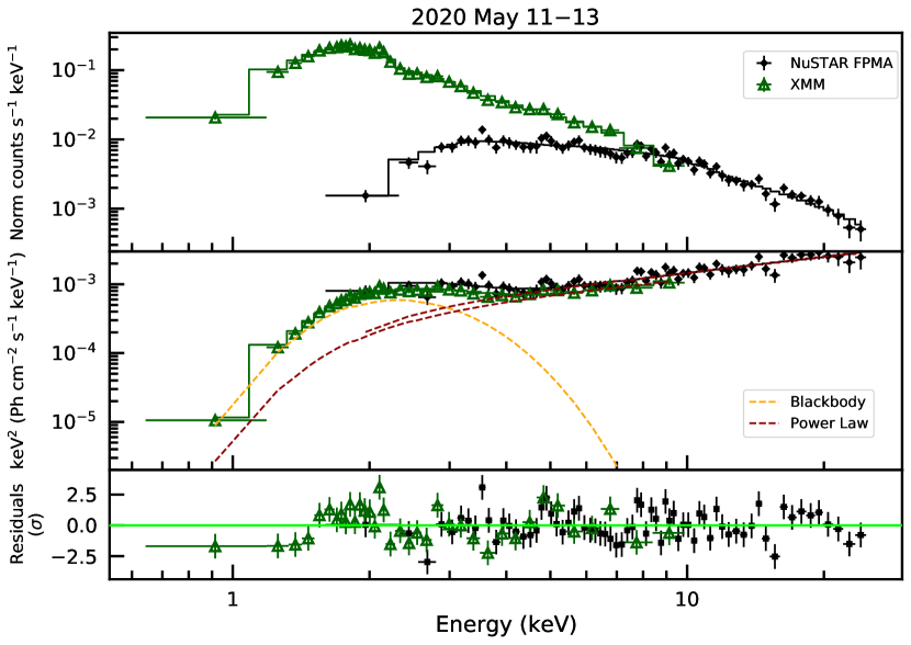
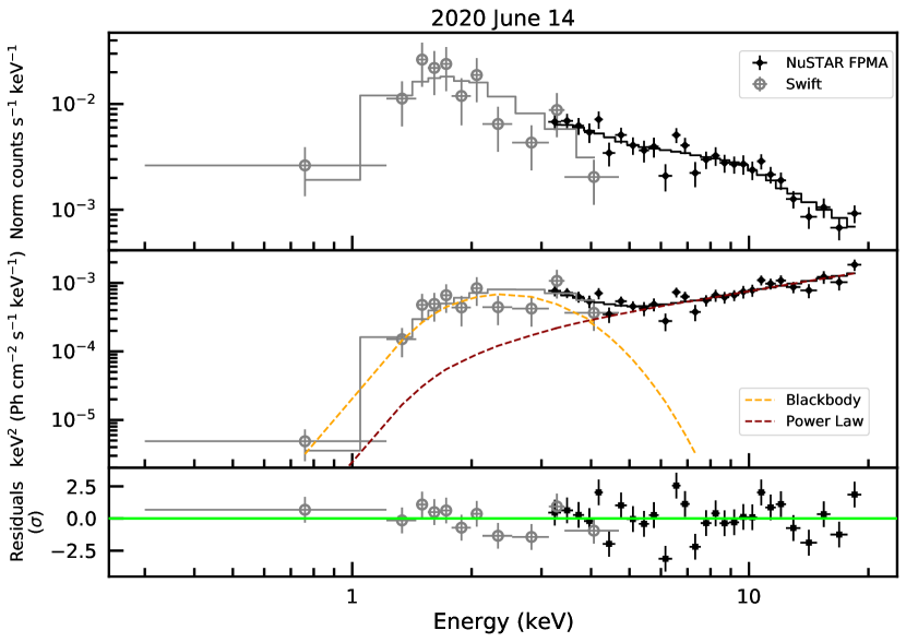
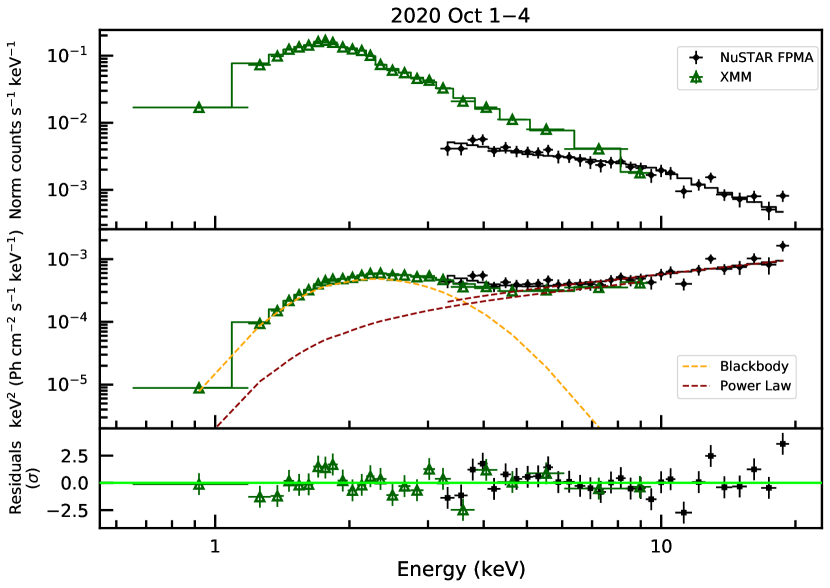
We start the fitting procedure by modelling the broadband spectra for the epochs 2020 May 11–13333We fit jointly the spectra extracted from the observations XMM–Newton ID 0871190201 and NuSTAR ID 80602313004. The latter was already presented in our previous work (Borghese et al., 2020)., June 14 and October 1–4. For each epoch, we fit the spectra jointly, forcing the model parameters to be the same across the data sets. Moreover, we include a multiplicative normalization which was frozen to one for the NuSTAR/FPMA spectrum, and allowed to vary for the other instruments. This term takes into account cross-calibration uncertainties between different instruments. Similarly as in the early stages of the outburst (Borghese et al., 2020), the spectra are well described by an absorbed blackbody plus a power-law component (BB+PL; see Figure 2). The best-fitting parameters are listed in Table 4, where we also include the results of the broadband spectral analysis of the observations performed close to the outburst onset (2020 May 2). The 0.3–20 keV luminosity decreased from (4.0 0.3) 1034 erg s-1 on 2020 May 2 to (2.3 0.1) 1034 erg s-1 on Oct 1–4, with a contribution of the power-law component of 75% and 45% respectively, in the same energy band ( is the source distance in units of 6.6 kpc). We did not detect a clear time evolution of the photon index , which attained a value of 1.2, and of the radius of the thermal emitting region, with an average value of 1.4 km. On the other hand, the PL normalization decreased by a factor of 2.5 and decreased from 0.59 keV to 0.440.01 keV during the time span covered by the broadband observations (2020 May 2 – October 4).
We then fit the same model to the Swift/XRT spectra jointly, freezing the to the above value. We allowed the other parameters to vary, although the photon index was not constrained over the energy range covered by Swift. Hence, we fixed this parameter to =1.2, that is, the averaged value derived from the broadband spectral analysis including NuSTAR spectra. The same procedure was applied to the NICER spectra. To increase the source signal-to-noise, we fitted together NICER spectra extracted from observations performed a few days apart, tying up all model parameters (see Table 2). Given the limited energy interval (1–5 keV), was frozen to 1.2 in this fit as well. We obtained a W-stat = 856.55 for 881 degrees of freedom (d.o.f.) for the Swift data and / = 3092.3 for 2495 d.o.f. for the NICER data sets.
For the Chandra spectra, we estimated a pile-up fraction of 13–18%. To correct for this effect, we included the multiplicative pile-up model (Davis, 2001), as implemented in Xspec, in the spectral fitting procedure. Following ‘The Chandra ABC guide to Pileup’444See http://cxc.harvard.edu/ciao/download/doc/pileup_abc.pdf., we allowed the grade migration parameter to vary and fixed the parameter psffrac equal to 0.95, that is, we assumed that 95% of events are contained within the central, piled-up portion of the source point spread function. We fit simultaneously the three spectra adopting an absorbed BB+PL model corrected by the pile-up model. As before, we fixed =2.3 1022 cm-2 and =1.2. The fit yielded = 177.83 for 181 d.o.f.
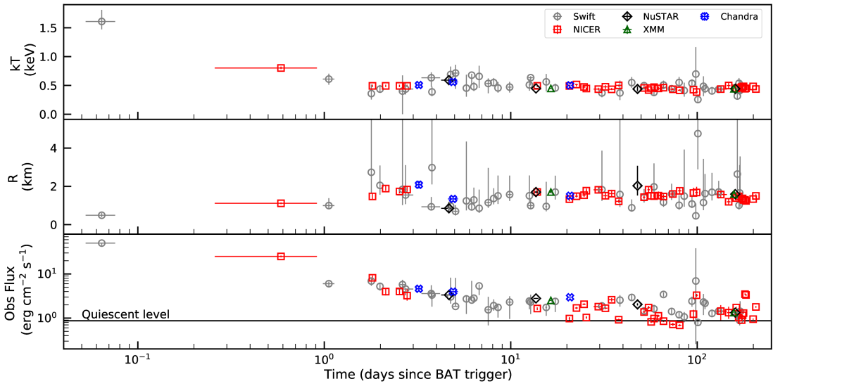
The best-fitting values for the radius and temperature of the blackbody component and the total observed flux (0.3–10 keV) corresponding to each observation are reported in Table 2. Figure 3 shows the temporal evolution of these quantities. After an initial rapid decrease over the course of a few days, the blackbody temperature settled on a steady value of 0.45 keV; while the blackbody radius did not show a strong variability, attaining an average value of 1.6 km during the 200 days covered by the monitoring campaign. These values are consistent with those derived for the BB component during the previous outbursts, when the soft (10 keV) spectra were described by a BB+PL model and did not show any spectral variability, except for the brightness (Younes et al., 2017). Moreover, they are compatible also with the averaged spectral parameters of the BB component ( 0.45 keV and 1.5 km) as obtained from NICER observations carried out during 2017–2019 (Younes et al., 2020).
3.2.2 Quiescent level
The quiescent level of SGR J1935 is still unknown. In our previous work (Borghese et al., 2020), we assumed the value derived from the Swift/XRT observation performed 4 days before the outburst onset (ID 00033349044; 2020 April 23). The source signal-to-noise ratio was not high enough to perform a sensitive spectral analysis, therefore we used WebPIMMS to derive an estimate of the observed flux, 4.510-13 erg cm-2 s-1 (0.3–10 keV; assuming a BB spectrum with =2.31022 cm-2 and =0.5 keV). Younes et al. (2020) used the average obtained from the NICER 2017–2019 monitoring campaign as a flux reference value (6.710-13 erg cm-2 s-1 adopting a BB model with =2.41022 cm-2, =0.45 keV and unabsorbed flux of 210-12 erg cm-2 s-1; 0.3–10 keV). Finally, Coti Zelati et al. (2018) performed a systematic spectral study of the major magnetar outbursts occurred up to the end of 2016 and identified the quiescent level of SGR J1935 with the flux measured in the XMM–Newton observation performed on 2014 October 4, (8.60.2)10-13 erg cm-2 s-1 (0.3–10 keV; 2BB). XMM–Newton/EPIC provides the most accurate characterization of the spectrum of SGR J1935 at the faint flux levels observed outside the outburst episodes. Hence, we deem that the last observation provides the most reliable approximation to the true quiescent level for this source. To be consistent with our analysis, we re-fit the XMM–Newton/EPIC-pn spectrum with a BB+PL model freezing =2.31022 cm-2. The fit gave an overall satisfactory description with keV, km and ( = 25.8 for 27 d.o.f.). We estimated the quiescent level of the observed flux to be equal to (8.70.3)10-13 erg cm-2 s-1, that corresponds to a quiescent luminosity of (1.30.1)1034 erg s-1 (0.3–10 keV).
| Epoch | Norm PL | Fluxa (Obs / Unabs) | Fluxa Unabs BB / PL | /d.o.f. | |||
|---|---|---|---|---|---|---|---|
| (keV) | (km) | (pho keV-1 cm-2 s-1) | (10-12 erg cm-2 s-1) | ||||
| 2020 May 2b | 0.59 | 0.85 | 1.170.06 | (2.50.4)10-4 | 5.80.1 / 7.80.6 | 2.20.5 / 5.60.2 | 148.4/139 |
| 2020 May 11–13 | 0.450.01 | 1.70.1 | 1.240.04 | (2.50.2)10-4 | 5.20.1 / 7.90.2 | 2.80.1 / 5.10.1 | 232.9/232 |
| 2020 Jun 14b | 0.440.04 | 2.0 | 1.070.11 | (9.12.1)10-5 | 3.40.1 / 6.20.5 | 3.71.3 / 2.50.1 | 53.17/49 |
| 2020 Oct 1–4 | 0.440.01 | 1.60.1 | 1.230.07 | (9.91.4)10-5 | 2.50.1 / 4.40.2 | 2.40.1 / 1.90.1 | 184.6/152 |
-
a
The fluxes are estimated in the 0.3–20 keV energy range.
-
b
For these two epochs, the NuSTAR spectrum is fitted together with a Swift spectrum taken almost simultaneously. For the latter, the W-stat=7 for 7 d.o.f. for May 2 and W-stat=6.8 for 10 d.o.f. for Jun 14.
3.2.3 Phase-resolved spectroscopy
We performed a phase-resolved spectral analysis using the two XMM–Newton/EPIC-pn data sets, where we detected the source spin period signal with high significance. We extracted spectra from three phase intervals (see Figure 1, bottom panels) and fitted them using an absorbed BB+PL model. Similarly to the phase-averaged spectral analysis, the column density was held fixed at = 2.31022 cm-2 for all the fits.
Firstly, for each epoch, we allowed only the normalizations of each component to vary, while the blackbody temperature and photon index were frozen at their best-fitting values for the corresponding phase-averaged spectrum (see Table 4). The fit yielded = 206.9 for 159 d.o.f. and = 187.9 for 169 d.o.f. for the data sets acquired on 2020 May 13 and October 1, respectively. We obtained statistically equivalent fits by allowing all parameters to vary among the phase-resolved spectra, with = 205.1 for 153 d.o.f. (2020 May) and 179.8 for 163 d.o.f. (2020 October). The best-fitting values are listed in Table 5. The blackbody radius and temperature do not show significant variations with the spin phase, while some hints for a phase dependence of the power-law index may be present.
| 2020 May 13 | |||
| Phase | |||
| (keV) | (km) | ||
| I | 0.470.01 | 1.60.1 | 0.9 |
| II | 0.450.01 | 1.50.1 | 1.00.2 |
| III | 0.430.02 | 1.60.1 | 1.40.2 |
| 2020 Oct 1 | |||
| Phase | |||
| (keV) | (km) | ||
| I | 0.440.01 | 1.50.1 | 1.20.3 |
| II | 0.460.01 | 1.40.1 | 0.90.3 |
| III | 0.430.01 | 1.50.1 | 1.20.3 |
3.3 Burst Search and Spectral Modelling
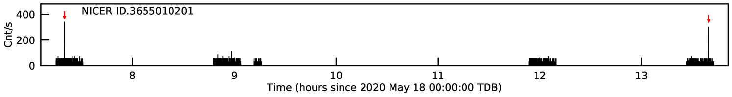
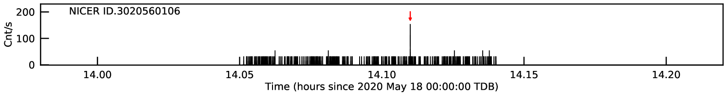
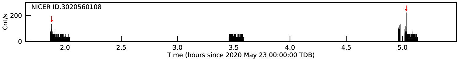
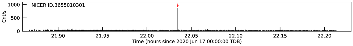
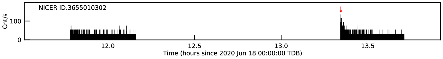
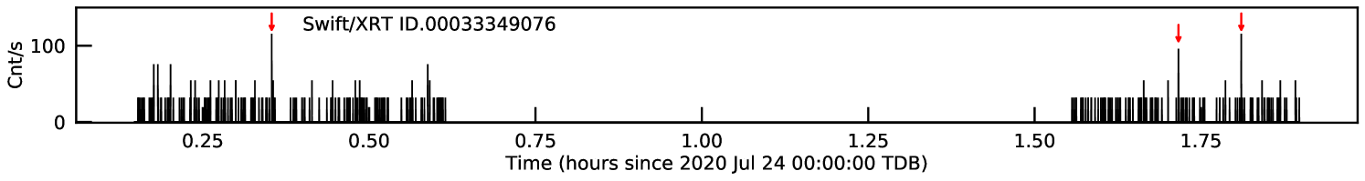
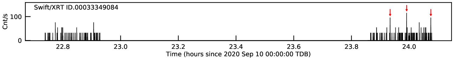
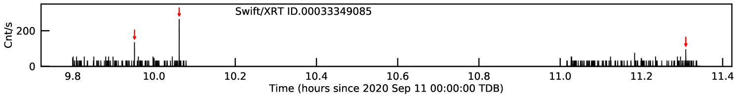
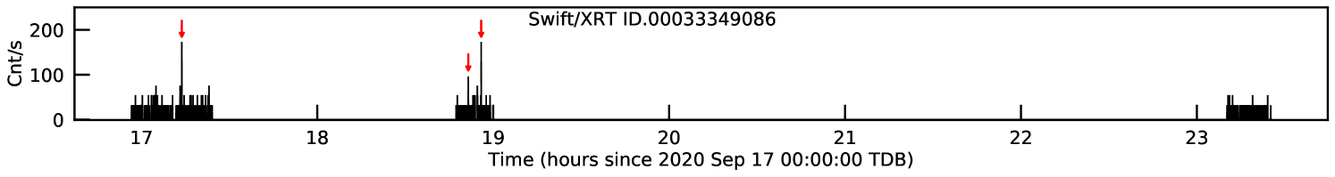
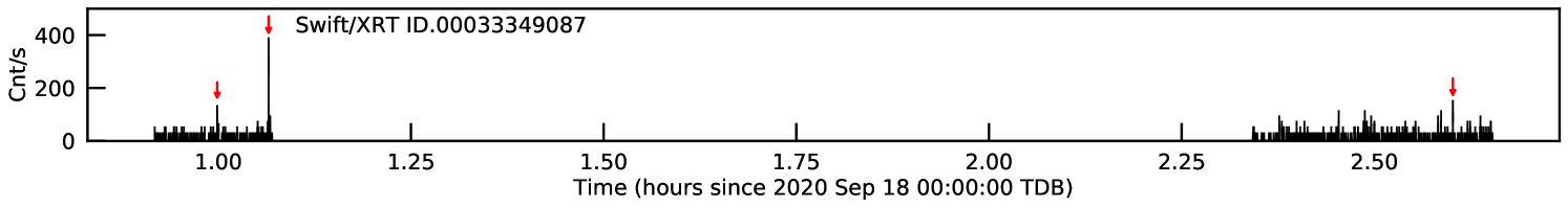
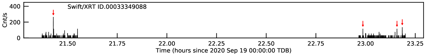
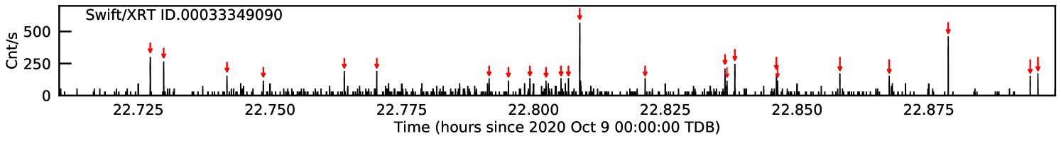
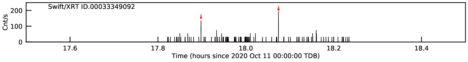
A search for short X-ray bursts was performed on all available data sets, using the same method outlined by Borghese et al. (2020) (see also, e.g., Gavriil et al. 2004). We extracted the time series with time resolutions of 2.5073 s for the Swift/XRT PC-mode data, of 73.36 ms for the XMM–Newton/EPIC-pn data sets, and of 1/16, 1/32 and 1/64 s in all other cases. We labelled as bursts the bins with a probability 10-4()-1, where is the total number of time bins in a given light curve and corresponds to the number of timing resolutions used in the search. In Table 7, we list the epochs of the bursts referred to the Solar system barycenter and Figure 6 displays their light curves.
On 2020 October 8–9, SGR J1935 entered a new radio active phase with the detection of multiple radio bursts and, for the first time, of pulsed radio emission at the X-ray spin period (Good & Chime/Frb Collaboration, 2020; Zhu et al., 2020). On 2020 October 9, Swift/XRT observed the source for 2.5 ks and we detected 24 bursts clustered within about ten minutes, corresponding to a burst rate of 0.04 burst s-1. Unfortunately, no meaningful spectral analysis could be carried out on the bursts detected using Swift/XRT owing to severe pile-up and saturation effects at the measured count rates.
On the other hand, meaningful spectra could be extracted for a couple of bursts detected by NICER, that is, those dubbed 3655010201 #2 and 3655010301 #1 in Table 7 (these are actually the events with the largest number of counts among the NICER sample; see also Table 8). For these events, the background level was estimated from the persistent emission detected in a close-in-time 10-s chunk of the data sets and the spectra were grouped to contain a minimum of 3 counts per spectral bin, allowing us to use the -statistic. The averaged spectra of these bursts were then fitted with an absorbed power-law model, fixing the column density to = 2.3 1022 cm-2. We obtained the following best-fitting parameters: and averaged unabsorbed flux erg cm-2 s-1 (0.3–10 keV) for burst 3655010201 #2 (W-stat = 4.90 for 9 d.o.f.); 0.3 and erg cm-2 s-1 (0.3–10 keV) for burst 3655010301 #1 (W-stat = 46.83 for 42 d.o.f.).
No significant bursts were detected in the XMM–Newton/EPIC-pn light curves.
4 Simultaneous radio observations
SGR J1935 was observed with the Sardinia Radio Telescope (SRT; Bolli et al. 2015; Prandoni et al. 2017) at 1.5 GHz in 2020 on October 9 and 10, simultaneously with NICER, for two consecutive 1.3-hr sessions each day (see Table 2 for details). Data were recorded with the ATNF digital backend PDFB3555See http://www.srt.inaf.it/media/uploads/astronomers/dfb.pdf in search mode over a bandwidth of 460 MHz split into 1 MHz channels. Total intensity data were 2-bit sampled every 100 s, except for the first half of the October 10 run, where full Stokes data were recorded every 256 s (the backend showed signs of overheating and the previous configuration was restored for the second part of the run).
The data were folded (with the software dspsr; van Straten & Bailes 2011) using the ephemeris obtained from X-ray data and using a dispersion measure DM = 332.8 pc cm-3 (Andersen et al., 2020), and blindly searched (with the package presto666https://github.com/scottransom/presto; Ransom 2011) over a DM range from 300 to 360 pc cm-3. A search spanning ms around the nominal period of the pulsar and the same DM range as the blind search was done on the folded data using pdmp (from the software package psrchive; Hotan et al. 2004). No persistent radio pulsations were found down to a flux density limit of mJy.
A search for single pulses was performed on the data using the spandak pipeline777https://github.com/gajjarv/PulsarSearch (Gajjar et al., 2018) The pipeline uses rfifind from the presto package for high-level radio frequency interference (RFI) excision. The search for bursts/single pulses is conducted through Heimdall (Barsdell et al., 2012) to quickly search across a DM range from 0 to 1000 pc cm-3. The de-dispersed time-series were searched for pulses using a matched-filtering technique with a maximum window size of 400 ms. Each candidate found by Heimdall at DMs within the range 300–400 pc cm-3 was scrutinized against all other candidates for each given observation to validate and identify only the genuine ones. A single candidate not resembling RFI was found at a DM compatible with that of the previously observed bursts (see e.g. Kirsten et al. 2021): DM = 332.42 pc cm-3. The candidate had a signal-to-noise ratio . In order to verify the genuineness of this candidate, a 1-s segment of data around the candidate has been reprocessed with an ad-hoc program with more sensitive RFI excision procedures taking into account lower level RFI. Firstly, a search for the most corrupted frequency channels in the DM zero data was carried out using the spectral kurtosis algorithm (Nita et al., 2016) as provided by the software package your888https://github.com/thepetabyteproject/your/ (Aggarwal et al., 2020). We used a spectral kurtosis thresholding of . Subsequently, we applied baseline subtraction and the data were normalized for the average bandpass. A check for possible corrupted temporal bins due to the presence of impulsive RFI was then performed with inter-quantile range (IQR) mitigation, similarly to Rajwade et al. (2020). The reprocessed data were then de-dispersed to the derived DM and smoothed via a 2-dimensional Gaussian filter. After this cleaning procedure, the candidate did not display any FRB-like characteristics either in the dynamic spectrum, or in the DM vs time plot, and we concluded that it was originated by RFI corrupted data. With no candidates found, we set an upper limit of 800 mJy on the fluence of a ms-long burst happening during these observations.
Since the data are uncalibrated, all upper limits reported above have been estimated using the modified radiometer equation (see e.g. Lorimer & Kramer 2004) adopting an antenna gain of 0.55 K/Jy, a system temperature of 35 K, a sky temperature of 25 K (accounting also for the supernova remnant hosting SGR J1935), a threshold of 7, and, for the periodic emission, a duty cycle of 5%.
5 Discussion
On 2020 April 27, SGR J1935 entered its fifth recorded outburst phase, placing itself in the short list of magnetars showing recurrent outbursts and frequent bursting activity, including e.g., 1E 1048.15937, SGR 162741 and CXOU J16474552 (An et al., 2018; Borghese et al., 2019; Archibald et al., 2020). This latest outburst stood out from the previous events experienced by SGR J1935 because it was accompanied by a remarkable X-ray burst forest (with more than 200 bursts detected in 20 minutes; Younes et al. 2020), and the emission of an intense radio burst with properties resembling those of FRBs and a X-ray counterpart (e.g., Andersen et al., 2020; Mereghetti et al., 2020).
Here we presented the temporal evolution of the spectral and timing properties of the source as tracked by an intensive X-ray monitoring campaign over 200 days since the outburst onset, as well as simultaneous radio observations.
5.1 Light curve modelling
To characterise the post-outburst luminosity decay, we modelled the temporal evolution of the 0.3–10 keV luminosity with a phenomenological model consisting of a constant and two exponential functions:
| (1) |
where is the quiescent level, is the epoch of the outburst onset and the -folding time can be considered as an estimate of the decay timescale. We fixed to MJD 58966.7683 (2020 April 27, 18:26:20 UTC), that is, the epoch at which Swift/BAT triggered on the first burst emitted from SGR J1935 during this latest active period (Barthelmy et al., 2020). For the quiescent luminosity, we assumed the value derived fitting a BB+PL model to the spectrum extracted from the XMM–Newton observation performed on 2014 October 4, (1.30.1)1034 erg s-1 (see Sec. 3.2.2). A 10 per cent error was assigned to each luminosity. The best-fitting values for the -folding times are =0.620.09 d and =31.23.5 d, highlighting an initial fast decay followed by a slower decrease. The source reached quiescence about 80 days after the outburst onset, releasing an energy of 5.81040 erg. Note that the quiescent level of SGR J1935 is not known yet and the true value could be lower than that assumed in this work. Therefore, the released energy and decay timescales should only be considered as a rough estimate. Younes et al. (2020) modelled the flux evolution over a period of three months after the outburst onset. Similar to our results, they found two decay trends described by very different -folding times. The initial rapid decay is characterized by =0.650.08 d, which is consistent with our findings. However, the long-term flux decay has an -folding time of =755 d, which differs from our results. The discrepancy might be due to the different quiescent level we assumed (see Sec. 3.2.2) and/or to the fact that our monitoring campaign extends over a longer period.
Younes et al. (2017) derived the energy emitted for the previous four outbursts within 10 days since the onset (see Table 5 of their paper). The energy released in the first 10 days of the 2020 outburst is equal to 2.61040 erg, second only to the 2016 June event when the energy was estimated to be 3.61040 erg. For the first two outbursts in 2014 and 2015, the emitted energy in the first 10 days was 1.21040 erg, while for the 2016 May episode it was slightly higher, 21040 erg.
Overall, the values for the decay timescale and the total energy released for the latest outburst of SGR J1935 fall at the low end of the range of values measured for magnetar outbursts. As a matter of fact, the decay time scale of 30 d is among the shortest measured so far. Yet, they are still compatible with the trend of the correlation measured previously, according to which the shorter the outburst, the less energetic. These results imply that the decay pattern of this outburst is not dissimilar from those observed in other magnetars (Coti Zelati et al., 2018).
| Epoch | Norm | |||
|---|---|---|---|---|
| (keV) | (rad) | |||
| May 2 | 0.670.05 | 0.610.04 | 0.490.01 | 0.0260.002 |
| May 11 | 0.480.01 | 0.650.02 | 0.4520.002 | 0.0340.001 |
| Jun14 | 0.500.03 | 0.720.06 | 0.430.01 | 0.0300.005 |
| Oct 1 | 0.480.01 | 0.710.04 | 0.4230.002 | 0.0240.001 |
5.2 Spectral evolution
About five days after its reactivation, SGR J1935 was observed with NuSTAR and Swift, revealing a hardening of the spectrum with the appearance of a non-thermal component extending up to 25 keV. In the following months, three additional broadband observations were performed and still detected hard X-ray emission till 20 keV. At each epoch, the non-thermal component was well modeled by a PL with a photon index of 1.2. Its contribution to the total 0.3–20 keV luminosity decreased from 75% at the outburst peak to 45% after 5 months (Table 4). During the whole monitoring campaign, besides the PL component, a blackbody was required to properly model the spectrum. Its temperature rapidly decayed during the first day of the outburst from 1.5 keV to 0.6 keV and decreased only slightly down to 0.45 keV over the following months. The corresponding emitting area was rather steady in time, with a radius of 1.6 km (Figure 3).
The spectral hardening and the detection of a power law at hard X-rays are ubiquitous properties of magnetars in outburst. The decomposition of the spectral model as a blackbody plus a power-law component is generally interpreted in terms of thermal emission from the cooling neutron star surface that gets affected by physical mechanisms taking place in the magnetosphere, such as Resonant Cyclotron Scattering (RCS; see e.g., Nobili et al., 2008a). The thermal photons produced at the surface gain energy via repeated scatterings onto charged particles flowing along the magnetic field lines, leading to the formation of a tail at higher energies. During an outburst, magnetic stresses and instabilities induce crustal displacements that can implant a strong twist of the magnetic field lines. The detection of a hot spot suggests that the magnetic twist is localized to a restricted portion of the magnetosphere, most likely to a current-carrying bundle of field lines (Beloborodov, 2009).
However, explaining the spectral evolution of SGR J1935 along the outburst within the RCS scenario poses some challenges. In fact, while the blackbody temperature quickly drops as expected (Beloborodov, 2009; Pons & Rea, 2012), the blackbody radius undergoes little changes and, even more strikingly, the power-law index remains almost constant. Actually, as recent 3D simulations have shown, the heated region can indeed cool without much shrinking (De Grandis et al., 2021) but the power-law should become softer as the twist subsides (Beloborodov, 2009). To investigate this further, we fitted the spectra with the NTZ model (Nobili et al., 2008a, b), which accounts for resonant cyclotron up-scattering of the soft seed photons (see Table 6). Taken at face value, the results of the NTZ spectral fits seem to indicate that, while the luminosity of the source is decaying, the decrease in the twist angle is accompanied by an increase in the velocity of the magnetospheric charges. Since both these quantities control the efficiency of the scattering process and hence the steepness of the power-law tail, this may in turn result in a nearly constant power-law index. The decrease in flux of the non-thermal component may reflect the fact that a smaller fraction of the photons from the thermal emitting area is intercepted by the currents in the bundle.
5.3 Timing properties and pulse profile simulations
Regarding the timing properties, we detected the spin period signal in the two XMM–Newton data sets (2020 May 13 and October 1). The pulse profile displays a variable morphology with energy. In the 5–10 keV interval, the profile exhibits a double-peaked shape, as observed in the previous NuSTAR observations performed close to the outburst onset (Borghese et al., 2020); while it evolves to a nearly sinusoidal shape at lower energies. The broadband pulsed fraction decreased by a factor of 2 between the two epochs. These behaviours are at odds with that observed during the first months of the 2014 outburst, when the pulse profile attained a quasi-sinusoidal shape, with no variation in time and energy, and the broadband pulsed fraction was in the 17–21 % range. These differences may suggest that distinct regions on the neutron star surface are heated during each outburst. By combining the two XMM–Newton spin period measurements with those presented by Borghese et al. (2020) ( = 3.24731(1) s on 2020 April 29–30, 3.247331(3) s on May 2 and 3.24731(1) s on May 11), we inferred a long-term average spin-down rate equal to = 3.5(1)10-11s s-1, that is a factor 2.5 larger than the measured in 2014 (=1.43(1)10-11s s-1; Israel et al. 2016). Changes in the pulse profile morphology and in the timing parameters are common during magnetar outbursts, mirroring the magnetosphere variations that follow flaring activity (for a more detailed discussion about the timing behavior of SGR J1935 during 2020 October 1 and November 27 see Younes et al., to be subm.).
Pulsations below keV were detected in both XMM–Newton pointings with a pulsed fraction of on 2020 May 13 and on October 1 (this value is however compatible with zero at the 3 level; Figure 1), and the unabsorbed BB flux decreased of about between the two epochs (Table 4). The low measured pulsed fraction is consistent with the (nearly) constant values of the BB parameters over the pulse phase, as derived from the phase-resolved spectroscopy (Section 3.2.3 and Table 5). To gain some insight on the source geometry and on its evolution over the outburst decay, we introduce a simple model according to which thermal photons are produced by a circular cap on the star surface heated at the outburst onset. We assume that the cap is at uniform temperature, as suggested by the lack of multiple BB components in the observed spectrum (this is at variance with, e.g., the case of XTE J1810197, Borghese et al., 2021). The cap properties are fixed by the measured blackbody temperature ( keV) and radius ( km which results in a semi-aperture for km); these values are representative of both the XMM–Newton observations of 2020 May 13 and October 1 since they do not change significantly between the two epochs. We computed the pulse profiles of the thermal component, as seen by an observer at infinity, as a function of the two geometrical angles and which measure the inclination of the line-of-sight (LOS) and of the cap axis with respect to the rotation axis, respectively. General-relativistic effects are taken into account (see Turolla & Nobili, 2013, for details)999Interstellar absorption and the detector response function were not accounted for. However, for the particular case we are dealing with (a constant temperature blackbody which changes in phase because of the varying visible area), the pulse profile is independent on both effects and the pulsed fraction is independent on the blackbody temperature.. Results for the pulsed fraction are shown in Figure 4 where the green/white, labeled contour marks the value of the pulsed fraction derived in the XMM observation ID 0871190201 (2020 May 13) and ID 0871191301 (2020 Oct 1), and respectively; the dashed contours are drawn in correspondence to errors. Results are not particularly constraining for the source geometry. However, we note that despite the fact that no significant changes in the emission properties of the hot spot were detected, the two values of the PF do not appear to be consistent, at least within uncertainties. While this can simply reflect measurement errors, taken face value it may suggest that the hot spot (slightly) changed its position on the surface without sensible variations in size and temperature.
During the X-ray monitoring campaign, the SRT observed SGR J1935 twice, on 2020 October 9 and 10, after the detection of three additional radio bursts by CHIME on October 8 (Good & Chime/Frb Collaboration, 2020). Moreover, on October 9, the FAST telescope detected multiple radio pulses with fluence up to 40 mJy ms and pulsed radio emission at a period of 3.24 s. During the SRT observations, we did not detect either pulsed emission or radio bursts, setting an upper limit on the flux density for the former of 0.1 mJy and on the fluence for the latter of 800 mJy ms. Furthermore, a dedicated multi-frequency campaign was initiated with multiple radio facilities after the 2020 April FRB-like radio burst (Bailes et al., 2021) without any successful detections. This phenomenology indicates that SGR J1935 can swing between a radio-loud and a radio-quiet states, although the connection with the X-ray activity currently remains not well understood and will need to be investigated with more coordinated radio and X-ray observations.
| Instrument | Obs.IDa | Burst epoch |
|---|---|---|
| YYYY-MM-DD hh:mm:ss (TDB) | ||
| NICER/XTI | 3655010201 #1 | 2020-05-18 07:19:55 |
| #2 | 13:39:39 | |
| NICER/XTI | 3020560106 #1 | 2020-05-20 14:06:36 |
| NICER/XTI | 3020560108 #1 | 2020-05-23 01:52:53 |
| #2 | 05:01:59 | |
| NICER/XTI | 3655010301 #1 | 2020-06-17 22:02:05 |
| NICER/XTI | 3655010302 #1 | 2020-06-18 13:20:40 |
| Swift/XRT (WT) | 00033349076 #1 | 2020-07-24 00:21:13 |
| #2 | 01:42:58 | |
| #3 | 01:48:38 | |
| Swift/XRT (WT) | 00033349084 #1 | 2020-09-10 23:56:02 |
| #2 | 23:59:28 | |
| #3 | 00:04:29 | |
| Swift/XRT (WT) | 00033349085 #1 | 2020-09-11 09:57:07 |
| #2 | 10:03:43 | |
| #3 | 11:18:33 | |
| Swift/XRT (WT) | 00033349086 #1 | 2020-09-17 17:13:47 |
| #2 | 18:51:31 | |
| #3 | 18:55:54 | |
| Swift/XRT (WT) | 00033349087 #1 | 2020-09-18 00:59:54 |
| #2 | 01:03:55 | |
| #3 | 02:36:07 | |
| Swift/XRT (WT) | 00033349088 #1 | 2020-09-19 21:25:43 |
| #2 | 22:59:11 | |
| #3 | 23:09:29 | |
| #4 | 23:11:05 | |
| Swift/XRT (WT) | 00033349090 #1 | 2020-10-09 22:43:38 |
| #2 | 22:43:47 | |
| #3 | 22:44:30 | |
| #4 | 22:44:55 | |
| #5 | 22:45:51 | |
| #6 | 22:46:13 | |
| #7 | 22:47:29 | |
| #8 | 22:47:43 | |
| #9 | 22:47:58 | |
| #10 | 22:48:08 | |
| #11 | 22:48:19 | |
| #12 | 22:48:24 | |
| #13 | 22:48:31 | |
| #14 | 22:49:16 | |
| #15 | 22:50:10 | |
| #16 | 22:50:12 | |
| #17 | 22:50:17 | |
| #18 | 22:50:46 | |
| #19 | 22:50:47 | |
| #20 | 22:51:29 | |
| #21 | 22:52:03 | |
| #22 | 22:52:43 | |
| #23 | 22:53:39 | |
| #24 | 22:53:44 | |
| Swift/XRT (WT) | 00033349092 #1 | 2020-10-11 17:53:53 |
| #2 | 18:04:27 |
-
a
The notation #N corresponds to the burst number in a given observation.
6 Acknowledgments
AB thanks George Younes for useful discussions and suggestions. We thank the referee, T. Güver, for his helpful comments. This research is based on observations with Chandra (NASA), NICER (NASA), NuSTAR (CaltTech/NASA/JPL), Swift (NASA/ASI/UK), XMM–Newton (ESA/NASA) and the Sardinia Radio Telescope (SRT). We thank N. Schartel for approving a Target of Opportunity observation with XMM–Newton in the Director’s Discretionary Time, and the XMM–Newton SOC for carrying out the observation. We also thank the NICER, NuSTAR and Swift teams for promptly scheduling our observations as well as the CHIME/FRB collaboration and the NICER team for asking part of the observations presented in this work. The SRT is funded by the Department of University and Research (MIUR), ASI, and the Autonomous Region of Sardinia (RAS) and is operated as National Facility by the National Institute for Astrophysics (INAF). A.B. and F.C.Z. are supported by Juan de la Cierva fellowships. A.B., F.C.Z., and N.R. are supported by grants SGR2017-1383, PGC2018-095512-BI00, and the ERC Consolidator grant “MAGNESIA" (No. 817661). G.L.I., S.M., R.T. and A.T. acknowledge financial support from the Italian MUR through grant PRIN 2017LJ39LM, “UNIAM". G.L.I. also acknowledges funding from ASI-INAF agreements I/037/12/0 and 2017-14-H.O. This work was partially supported by the program Unidad de Excelencia María de Maeztu CEX2020-001058-M. We also acknowledge support from the PHAROS COST Action (CA16214). This research has made use of the following software: CIAO (v4.12; Fruscione et al. 2006, MARX (v5.5.1), SAS (v19; Gabriel et al. 2004); HEASoft (v6.28), FTOOLS (v6.28; Blackburn 1995), XSPEC (v12.11.0h; Arnaud 1996), NICERDAS (v7a), NuSTARDAS (v2.0.0), MATPLOTLIB (v3.2.1; Hunter 2007), NUMPY (v1.18.4; Harris et al. 2020).
7 Data availability
Radio data can be provided by the authors upon reasonable request. Data from NICER, Swift, XMM–Newton, Chandra and NuSTAR observations are publicly available.
References
- Aggarwal et al. (2020) Aggarwal K., et al., 2020, Journal of Open Source Software, 5, 2750
- An et al. (2018) An H., Cumming A., Kaspi V. M., 2018, ApJ, 859, 16
- Andersen et al. (2020) Andersen B. C., et al., 2020, Nature, 587, 54
- Archibald et al. (2020) Archibald R. F., Scholz P., Kaspi V. M., Tendulkar S. P., Beardmore A. P., 2020, ApJ, 889, 160
- Arnaud (1996) Arnaud K. A., 1996, in Jacoby G. H., Barnes J., eds, Astronomical Data Analysis Software and Systems V Vol. 101, XSPEC: The First Ten Years. ASP, San Francisco, pp 17–20
- Bailes et al. (2021) Bailes M., et al., 2021, MNRAS, 503, 5367
- Barsdell et al. (2012) Barsdell B. R., Bailes M., Barnes D. G., Fluke C. J., 2012, MNRAS, 422, 379
- Barthelmy et al. (2020) Barthelmy S. D., et al., 2020, GRB Coordinates Network, 27657, 1
- Beloborodov (2009) Beloborodov A. M., 2009, ApJ, 703, 1044
- Beloborodov (2017) Beloborodov A. M., 2017, ApJ, 843, L26
- Bera & Chengalur (2019) Bera A., Chengalur J. N., 2019, MNRAS, 490, L12
- Blackburn (1995) Blackburn J. K., 1995, in Shaw R. A., Payne H. E., Hayes J. J. E., eds, Astronomical Data Analysis Software and Systems IV. Vol. 77, FTOOLS: A FITS Data Processing and Analysis Software Package. ASP Conf. Ser., San Francisco, CA, p. 367
- Bochenek et al. (2020) Bochenek C. D., Ravi V., Belov K. V., Hallinan G., Kocz J., Kulkarni S. R., McKenna D. L., 2020, Nature, 587, 59
- Bolli et al. (2015) Bolli P., et al., 2015, Journal of Astronomical Instrumentation, 4, 1550008
- Borghese et al. (2019) Borghese A., et al., 2019, MNRAS, 484, 2931
- Borghese et al. (2020) Borghese A., Coti Zelati F., Rea N., Esposito P., Israel G. L., Mereghetti S., Tiengo A., 2020, ApJ, 902, L2
- Borghese et al. (2021) Borghese A., et al., 2021, MNRAS, 504, 5244
- Burrows et al. (2005) Burrows D. N., et al., 2005, Space Science Reviews, 120, 165
- Caleb & Keane (2021) Caleb M., Keane E., 2021, Universe, 7, 453
- Caleb et al. (2022) Caleb M., et al., 2022, MNRAS, 510, 1996
- Coti Zelati et al. (2018) Coti Zelati F., Rea N., Pons J. A., Campana S., Esposito P., 2018, MNRAS, 474, 961
- Davis (2001) Davis J. E., 2001, ApJ, 562, 575
- De Grandis et al. (2021) De Grandis D., Taverna R., Turolla R., Gnarini A., Popov S. B., Zane S., Wood T. S., 2021, ApJ, 914, 118
- Esposito et al. (2021) Esposito P., Rea N., Israel G. L., 2021, Magnetars: A Short Review and Some Sparse Considerations. Springer Berlin Heidelberg, Berlin, Heidelberg, pp 97–142, doi:10.1007/978-3-662-62110-3_3, https://doi.org/10.1007/978-3-662-62110-3_3
- Fruscione et al. (2006) Fruscione A., et al., 2006, in Silva D. R., Doxsey R. E., eds, SPIE Conference Series Vol. 6270, Observatory Operations: Strategies, Processes, and Systems. SPIE, Bellingham, p. 62701V, doi:10.1117/12.671760
- Gabriel et al. (2004) Gabriel C., et al., 2004, in Ochsenbein F., Allen M. G., Egret D., eds, Astronomical Data Analysis Software and Systems (ADASS) XIII Vol. 314, The XMM-Newton SAS - Distributed Development and Maintenance of a Large Science Analysis System: A Critical Analysis. San Francisco, CA: ASP, p. 759
- Gajjar et al. (2018) Gajjar V., et al., 2018, ApJ, 863, 2
- Garmire et al. (2003) Garmire G. P., Bautz M. W., Ford P. G., Nousek J. A., Ricker Jr. G. R., 2003, in Truemper J. E., Tananbaum H. D., eds, Proceedings of the SPIE. Vol. 4851, X-Ray and Gamma-Ray Telescopes and Instruments for Astronomy.. SPIE, Bellingham, pp 28–44, doi:10.1117/12.461599
- Gavriil et al. (2004) Gavriil F. P., Kaspi V. M., Woods P. M., 2004, ApJ, 607, 959
- Gendreau et al. (2012) Gendreau K. C., Arzoumanian Z., Okajima T., 2012, in Proc. SPIE. p. 844313, doi:10.1117/12.926396
- Good & Chime/Frb Collaboration (2020) Good D., Chime/Frb Collaboration 2020, The Astronomer’s Telegram, 14074, 1
- Göğü\textcommabelows et al. (2020) Göğü\textcommabelows E., et al., 2020, ApJ, 905, L31
- Harris et al. (2020) Harris C. R., et al., 2020, Nature, 585, 357
- Harrison et al. (2013) Harrison F. A., et al., 2013, ApJ, 770, 103
- Hotan et al. (2004) Hotan A. W., van Straten W., Manchester R. N., 2004, Publ. Astron. Soc. Australia, 21, 302
- Hunter (2007) Hunter J. D., 2007, Computing in Science & Engineering, 9, 90
- Israel & Stella (1996) Israel G. L., Stella L., 1996, ApJ, 468, 369
- Israel et al. (2016) Israel G. L., et al., 2016, MNRAS, 457, 3448
- Israel et al. (2021) Israel G. L., et al., 2021, ApJ, 907, 7
- Kaspi & Beloborodov (2017) Kaspi V. M., Beloborodov A. M., 2017, ARA&A, 55, 261
- Kirsten et al. (2020) Kirsten F., Snelders M. P., Jenkins M., Nimmo K., van den Eijnden J., Hessels J. W. T., Gawroński M. P., Yang J., 2020, Nature Astronomy,
- Kirsten et al. (2021) Kirsten F., Snelders M. P., Jenkins M., Nimmo K., van den Eijnden J., Hessels J. W. T., Gawroński M. P., Yang J., 2021, Nature Astronomy, 5, 414
- Lin et al. (2020a) Lin L., et al., 2020a, Nature, 587, 63
- Lin et al. (2020b) Lin L., Göğü\textcommabelows E., Roberts O. J., Baring M. G., Kouveliotou C., Kaneko Y., van der Horst A. J., Younes G., 2020b, ApJ, 902, L43
- Lorimer & Kramer (2004) Lorimer D. R., Kramer M., 2004, Handbook of Pulsar Astronomy. Cambridge, UK: Cambridge University Press
- Marcote et al. (2020) Marcote B., et al., 2020, Nature, 577, 190
- Margalit et al. (2020) Margalit B., Beniamini P., Sridhar N., Metzger B. D., 2020, ApJ, 899, L27
- Mereghetti et al. (2020) Mereghetti S., et al., 2020, ApJ, 898, L29
- Nita et al. (2016) Nita G. M., Gary D. E., Hellbourg G., 2016, in 2016 Radio Frequency Interference (RFI). pp 75–80, doi:10.1109/RFINT.2016.7833535
- Nobili et al. (2008a) Nobili L., Turolla R., Zane S., 2008a, MNRAS, 386, 1527
- Nobili et al. (2008b) Nobili L., Turolla R., Zane S., 2008b, MNRAS, 389, 989
- Palmer (2020) Palmer D., 2020, The Astronomer’s Telegram, 14208, 1
- Pons & Rea (2012) Pons J. A., Rea N., 2012, ApJ, 750, L6
- Prandoni et al. (2017) Prandoni I., et al., 2017, A&A, 608, A40
- Rajwade et al. (2020) Rajwade K., et al., 2020, in Evans C. J., Bryant J. J., Motohara K., eds, Vol. 11447, Ground-based and Airborne Instrumentation for Astronomy VIII. SPIE, pp 78 – 85, doi:10.1117/12.2559937, https://doi.org/10.1117/12.2559937
- Ransom (2011) Ransom S., 2011, PRESTO: PulsaR Exploration and Search TOolkit (ascl:1107.017)
- Ridnaia et al. (2021) Ridnaia A., et al., 2021, Nature Astronomy,
- Stamatikos et al. (2014) Stamatikos M., Malesani D., Page K. L., Sakamoto T., 2014, GRB Coordinates Network, 16520, 1
- Strüder et al. (2001) Strüder L., et al., 2001, A&A, 365, L18
- Tavani et al. (2021) Tavani M., et al., 2021, Nature Astronomy,
- Turner et al. (2001) Turner M. J. L., et al., 2001, A&A, 365, L27
- Turolla & Nobili (2013) Turolla R., Nobili L., 2013, ApJ, 768, 147
- Verner et al. (1996) Verner D. A., Ferland G. J., Korista K. T., Yakovlev D. G., 1996, ApJ, 465, 487
- Wilms et al. (2000) Wilms J., Allen A., McCray R., 2000, ApJ, 542, 914
- Younes et al. (2017) Younes G., et al., 2017, ApJ, 847, 85
- Younes et al. (2020) Younes G., et al., 2020, ApJ, 904, L21
- Zhang et al. (2020) Zhang C. F., et al., 2020, The Astronomer’s Telegram, 13699, 1
- Zhou et al. (2020) Zhou P., Zhou X., Chen Y., Wang J.-S., Vink J., Wang Y., 2020, arXiv e-prints, p. arXiv:2005.03517
- Zhu et al. (2020) Zhu W., et al., 2020, The Astronomer’s Telegram, 14084, 1
- van Straten & Bailes (2011) van Straten W., Bailes M., 2011, Publ. Astron. Soc. Australia, 28, 1
Appendix A NICER bursts: fluence and duration
In Table 8, we list the fluence and durations for the bursts detected in the NICER/XTI light curves. Owing to uncertainties related to the detector saturation limits, we do not report these quantities for the bursts identified in the Swift/XRT data sets.
In the table, the fluence refers to the 0.3–10 keV range and the duration has to be considered as an approximate value. We estimated it by summing the 15.625-ms time bins showing enhanced emission for the structured bursts, and by setting it equal to the coarser time resolution at which the burst is detected in all the other cases.
| Obs.ID | Burst epoch | Fluence | Duration |
|---|---|---|---|
| YYYY-MM-DD hh:mm:ss (TDB) | (counts) | (ms) | |
| 3655010201 #1 | 2020-05-18 07:19:55 | 11 | 62.5 |
| #2 | 13:39:39 | 15 | 62.5 |
| 3020560106 #1 | 2020-05-20 14:06:36 | 7 | 62.5 |
| 3020560108 #1 | 2020-05-23 01:52:53 | 6 | 31.25 |
| #2 | 05:01:59 | 7 | 62.5 |
| 3655010301 #1 | 2020-06-17 22:02:05 | 47 | 62.5 |
| 3655010302 #1 | 2020-06-18 13:20:40 | 6 | 62.5 |