Colouring Strong Products

Abstract

Recent results show that several important graph classes can be embedded as subgraphs of strong products of simpler graphs classes (paths, small cliques, or graphs of bounded treewidth). This paper develops general techniques to bound the chromatic number (and its popular variants, such as fractional, clustered, or defective chromatic number) of the strong product of general graphs with simpler graphs classes, such as paths, and more generally graphs of bounded treewidth. We also highlight important links between the study of (fractional) clustered colouring of strong products and other topics, such as asymptotic dimension in metric geometry and topology, site percolation in probability theory, and the Shannon capacity in information theory.

1 Introduction

The past few years have seen a renewed interest in the structure of strong products of graphs. One motivation is the Planar Graph Product Structure Theorem (see Section 1.2), which shows that every planar graph is a subgraph of the strong product of a graph with bounded treewidth and a path. As a consequence, results on the structure of planar graphs can be simply deduced from the study of the structure of strong products of graphs (and in particular from the study of the strong product of a graph with a path). This theorem was preceded by several results that can be also stated as product structure theorems (where the host graph is the strong product of paths, trees, or small complete graphs); see Section 1.2 below. Note that grids in finite-dimensional euclidean spaces can be expressed as the strong product of finitely many paths, and colouring properties of these grids are related to important topological or metric properties of these spaces; see Section 1.3 and Section 1.4.

It turns out that the study of colouring properties of strong products of graphs has interesting connections with various problems in combinatorics, which we highlight below. In particular, in order to understand the chromatic number (or the clustered or defective chromatic number) of strong products, it is very helpful to understand the fractional versions of such colourings, which have strong ties with site percolation in probability theory (see Section 1.6) and Shannon capacity in information theory (see Section 1.7).

We start with the definitions of various graph products, as well as various graph colouring notions that are studied in this paper. We then give an overview of our main results in Section 1.8.

1.1 Definitions

The cartesian product of graphs $A$ and $B$, denoted by $A\mathbin{\square}B$, is the graph with vertex set $V(A)\times V(B)$, where distinct vertices $(v,x),(w,y)\in V(A)\times V(B)$ are adjacent if: $v=w$ and $xy\in E(B)$, or $x=y$ and $vw\in E(A)$. The direct product of graphs $A$ and $B$, denoted by $A\times B$, is the graph with vertex set $V(A)\times V(B)$, where distinct vertices $(v,x),(w,y)\in V(A)\times V(B)$ are adjacent if $vw\in E(A)$ and $xy\in E(B)$. The strong product of graphs $A$ and $B$, denoted by $A\boxtimes B$, is the graph $(A\mathbin{\square}B)\cup(A\times B)$. For graph classes $\mathcal{G}_{\_}1$ and $\mathcal{G}_{\_}2$, let

$$\mathcal{G}_{\_}1\mathbin{\square}\mathcal{G}_{\_}2 :=\{G_{\_}1\mathbin{\square}G_{\_}2:G_{\_}1\in\mathcal{G}_{\_}1,G_{\_}2\in\mathcal{G}_{\_}2\}$$

$$\mathcal{G}_{\_}1\times\mathcal{G}_{\_}2 :=\{G_{\_}1\times G_{\_}2:G_{\_}1\in\mathcal{G}_{\_}1,G_{\_}2\in\mathcal{G}_{\_}2\}$$

$$\mathcal{G}_{\_}1\boxtimes\mathcal{G}_{\_}2 :=\{G_{\_}1\boxtimes G_{\_}2:G_{\_}1\in\mathcal{G}_{\_}1,G_{\_}2\in\mathcal{G}_{\_}2\}.$$

A colouring of a graph $G$ is simply a function $f:V(G)\to\mathcal{C}$ for some set $\mathcal{C}$ whose elements are called colours. If $|\mathcal{C}|\leqslant k$ then $f$ is a $k$-colouring. An edge $vw$ of $G$ is $f$-monochromatic if $f(v)=f(w)$. An $f$-monochromatic component, sometimes called a monochromatic component, is a connected component of the subgraph of $G$ induced by $\{v\in V(G):f(v)=\alpha\}$ for some $\alpha\in\mathcal{C}$. We say $f$ has clustering $c$ if every $f$-monochromatic component has at most $c$ vertices. The $f$-monochromatic degree of a vertex $v$ is the degree of $v$ in the monochromatic component containing $v$. Then $f$ has defect $d$ if every $f$-monochromatic component has maximum degree at most $d$ (that is, each vertex has monochromatic degree at most $d$). There have been many recent papers on clustered and defective colouring [57, 65, 36, 11, 23, 24, 19, 46, 33, 56, 48, 47, 50, 49, 51, 58, 20]; see [70] for a survey.

The general goal of this paper is to study defective and clustered chromatic number of graph products, with the focus on minimising the number of colours with bounded defect or bounded clustering a secondary goal.

The clustered chromatic number of a graph class $\mathcal{G}$, denoted by $\raisebox{1.55pt}{\scalebox{1.2}{$\chi$}}_{\star}(\mathcal{G})$, is the minimum integer $k$ for which there exists an integer $c$ such that every graph in $\mathcal{G}$ has a $k$-colouring with clustering $c$. If there is no such integer $k$, then $\mathcal{G}$ has unbounded clustered chromatic number. The defective chromatic number of a graph class $\mathcal{G}$, denoted by $\raisebox{1.55pt}{\scalebox{1.2}{$\chi$}}_{\Delta}(\mathcal{G})$, is the minimum integer $k$ for which there exists $c\in\mathbb{N}$ such that every graph in $\mathcal{G}$ has a $k$-colouring with defect $c$. If there is no such integer $k$, then $\mathcal{G}$ has unbounded defective chromatic number. Every colouring of a graph with clustering $c$ has defect $c-1$. Thus $\raisebox{1.55pt}{\scalebox{1.2}{$\chi$}}_{\Delta}(\mathcal{G})\leqslant\raisebox{1.55pt}{\scalebox{1.2}{$\chi$}}_{\star}(\mathcal{G})\leqslant\raisebox{1.55pt}{\scalebox{1.2}{$\chi$}}(\mathcal{G})$ for every class $\mathcal{G}$.

Obviously, for all graphs $G$ and $H$,

$$\max\{\chi(G),\chi(H)\}\leqslant\chi(G\boxtimes H)\leqslant\chi(G)\,\chi(H).$$

The upper bound is tight if $G$ and $H$ are complete graphs, for example. The lower bound is tight if $G$ or $H$ has no edges. However, Vesztergombi [66] proved that $\chi(G\boxtimes K_{\_}2)\geqslant\chi(G)+2$, implying that if $E(H)\neq\emptyset$ then

$$\chi(G\boxtimes H)\geqslant\chi(G)+2.$$

More generally, Klavžar and Milutinović [40] proved that

$$\chi(G\boxtimes H)\geqslant\chi(G)+2\omega(H)-2.$$

Žerovnik [68] studied the chromatic numbers of the strong product of odd cycles.

A classical result of Sabidussi [60] states that for any graphs $G$ and $H$, $\chi(G\Box H)=\max\{\chi(G),\chi(H)\}$, while a famous conjecture of Hedetniemi stated that $\chi(G\times H)=\min\{\chi(G),\chi(H)\}$. This conjecture was recently disproved by Shitov [63]. The remainder of the paper focuses on the strong product $\boxtimes$ of graphs rather than $\Box$ and $\times$.

1.2 Subgraphs of Strong Products

The study of colourings of strong products is partially motivated from the following results that show that natural classes of graphs are subgraphs of certain strong products. Thus, colouring results for the product imply an analogous result for the original class. Later in the paper we use Theorem 2, while Theorems 1 and 3 are not used. Nevertheless, these results provide further motivation for studying colouring of strong graph products, since they show that several classes with a complicated structure can be expressed as subgraphs of the strong product of significantly simpler graph classes.

For a graph $G$ and an integer $d\geqslant 1$, let $\boxtimes_{\_}dG$ denote the $d$-fold strong product $G\boxtimes\dots\boxtimes G$.

Theorem 1 ([44]).

For every $c\in\mathbb{N}$ there exists $d\in O(c\log c)$, such that if $G$ is a graph with $|\{w\in V(G):\operatorname{dist}(v,w)\leqslant r\}|\leqslant r^{c}$ for every vertex $v\in V(G)$ and integer $r\geqslant 2$, then $G\subseteq\boxtimes_{\_}dP$.

Theorem 2 ([13, 69, 15]).

Every graph with maximum degree $\Delta\in\mathbb{N}^{+}$ and treewidth less than $k\in\mathbb{N}^{+}$ is a subgraph of $T\boxtimes K_{\_}{20k\Delta}$ for some tree $T$ with maximum degree at most $20k\Delta^{2}$.

Theorem 3 ([16, 64]).

Every planar graph is a subgraph of:

1. $H\boxtimes P$ for some planar graph $H$ of treewidth at most $6$ and for some path $P$;

2. $H\boxtimes P\boxtimes K_{\_}3$ for some planar graph $H$ of treewidth at most $3$ and for some path $P$.

The interested reader is referred to [16, 17, 14, 34, 35, 10] for extensions of this result to graphs of bounded genus, and other natural generalisations of planar graphs.

1.3 Hex Lemma

The famous Hex Lemma says that the game of Hex cannot end in a draw; see [31] for an account of the rich history of this game. As illustrated in Figure 1, the Hex Lemma is equivalent to saying that in every 2-colouring of the vertices of the $n\times n$ triangulated grid, there is a monochromatic path from one side to the opposite side.

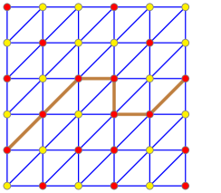
Figure 1: A Hex game.

This result generalises to higher dimensions as follows. Let $G_{\_}n^{d}$ be the graph with vertex-set $\{1,\dots,n\}^{d}$, where distinct vertices $(v_{\_}1,\dots,v_{\_}d)$ and $(w_{\_}1,\dots,w_{\_}d)$ are adjacent in $G^{d}_{\_}n$ whenever $w_{\_}i\in\{v_{\_}i,v_{\_}i+1\}$ for each $i\in\{1,\dots,d\}$, or $v_{\_}i\in\{w_{\_}i,w_{\_}i+1\}$ for each $i\in\{1,\dots,d\}$. Note that if each vertex $(v_{\_}1,\dots,v_{\_}d)$ is coloured $(\sum_{\_}iv_{\_}i)\bmod{(d+1)}$, then adjacent vertices $(v_{\_}1,\dots,v_{\_}d)$ and $(w_{\_}1,\dots,w_{\_}d)$ are assigned distinct colours, since $|(\sum_{\_}iv_{\_}i)-(\sum_{\_}iw_{\_}i)|\leqslant d$. Thus $\raisebox{1.55pt}{\scalebox{1.2}{$\chi$}}(G_{\_}n^{d})\leqslant d+1$. In fact, $\raisebox{1.55pt}{\scalebox{1.2}{$\chi$}}(G^{d}_{\_}n)=d+1$ since $\{(v_{\_}1,\dots,v_{\_}d),(v_{\_}1+1,v_{\_}2,\dots,v_{\_}d),(v_{\_}1+1,v_{\_}2+1,v_{\_}3,\dots,v_{\_}d),\dots,(v_{\_}1+1,v_{\_}2+1,\dots,v_{\_}d+1)\}$ is a $(d+1)$-clique. The $d$-dimensional Hex Lemma provides a stronger lower bound: in every $d$-colouring of $G_{\_}n^{d}$ there is a monochromatic path from one ‘side’ of $G^{d}_{\_}n$ to the opposite side [27]. Thus

$$\raisebox{1.55pt}{\scalebox{1.2}{$\chi$}}_{\star}(\{G^{d}_{\_}n:n\in\mathbb{N}\})=d+1.$$

See [27, 45, 54, 7, 54, 53, 37] for related results. For example, Gale [27] showed that this theorem is equivalent to the Brouwer Fixed Point Theorem.

These results are related to clustered colourings of strong products, as we now explain. Let $P_{\_}n$ denote the $n$-vertex path and $\boxtimes_{\_}dP_{\_}{n}$ be the $d$-dimensional grid $P_{\_}n\boxtimes\cdots\boxtimes P_{\_}n$. Then $G_{\_}n^{d}$ is a subgraph of $\boxtimes_{\_}dP_{\_}{n}$. So

$$\raisebox{1.55pt}{\scalebox{1.2}{$\chi$}}_{\star}(\{\boxtimes_{\_}dP_{\_}{n}:n\in\mathbb{N}\})\geqslant\raisebox{1.55pt}{\scalebox{1.2}{$\chi$}}_{\star}(\{G^{d}_{\_}n:n\in\mathbb{N}\})=d+1.$$

A corollary of our main result is that equality holds here. In particular, Corollary 25 shows that there is a $(d+1)$-colouring of $P^{\boxtimes d}_{\_}{n}$ with clustering $d!$. Thus

$$\raisebox{1.55pt}{\scalebox{1.2}{$\chi$}}_{\star}(\{\boxtimes_{\_}dP_{\_}{n}:n\in\mathbb{N}\})=d+1.$$

1.4 Asymptotic Dimension

Given a graph $G$ and an integer $\ell\geqslant 1$, $G^{\ell}$ is the graph obtained from $G$ by adding an edge between each pair of distinct vertices $u,v$ at distance at most $\ell$ in $G$. Note that $G^{1}=G$. We say that a subset $S$ of vertices of a graph $G$ has weak diameter at most $d$ in $G$ if any two vertices of $S$ are at distance at most $d$ in $G$.

The asymptotic dimension of a metric space was introduced by Gromov [29] in the context of geometric group theory. For graph classes (and their shortest paths metric), it can be defined as follows [8]: the asymptotic dimension of a graph class $\mathcal{F}$ is the minimum $m\in\mathbb{N}_{\_}0$ for which there is a function $f:\mathbb{N}\rightarrow\mathbb{N}$ such that for every $G\in\mathcal{F}$ and $\ell\in{\mathbb{N}}$, $G^{\ell}$ has an $(m+1)$-colouring in which each monochromatic component has weak diameter at most $f(\ell)$ in $G^{\ell}$. (If no such integer $m$ exists, the asymptotic dimension of $\mathcal{F}$ is said to be $\infty$).

Taking $\ell=1$, we see that graphs from any graph class $\mathcal{F}$ of asymptotic dimension at most $m$ have an $(m+1)$-colouring in which each monochromatic component has bounded weak diameter. If, in addition, the graphs in $\mathcal{F}$ have bounded maximum degree, then all graphs in $\mathcal{F}$ have $(m+1)$-colourings with bounded clustering [8], implying $\raisebox{1.55pt}{\scalebox{1.2}{$\chi$}}_{\star}(\mathcal{F})\leqslant m+1$.

It is well-known that the class of $d$-dimensional grids (with or without diagonals) has asymptotic dimension $d$ (see [29]), and since they also have bounded degree, it directly follows from the remarks above that $d$-dimensional grids have $(d+1)$-colourings with bounded clustering.

An important problem is to bound the dimension of the product of topological or metric spaces as a function of their dimensions. It follows from the work of Bell and Dranishnikov [6] and Brodskiy et al. [9] that if $\mathcal{F}_{\_}1$ and $\mathcal{F}_{\_}2$ are classes of asymptotic dimension $m_{\_}1$ and $m_{\_}2$, respectively, then the class $\mathcal{F}_{\_}1\boxtimes\mathcal{F}_{\_}2:=\{G_{\_}1\boxtimes G_{\_}2\,:\,G_{\_}1\in\mathcal{F}_{\_}1,G_{\_}2\in\mathcal{F}_{\_}2\}$ has asymptotic dimension at most $m_{\_}1+m_{\_}2$. For example, that $d$-dimensional grids have asymptotic dimension at most $d$ can be deduced from this product theorem by induction, using the fact that the family of paths has asymptotic dimension 1. In particular, if two classes $\mathcal{F}_{\_}1$ and $\mathcal{F}_{\_}2$ have asymptotic dimension $m_{\_}1$ and $m_{\_}2$, respectively, and have uniformly bounded maximum degree, then the graphs in $\mathcal{F}_{\_}1\boxtimes\mathcal{F}_{\_}2$ have $(m_{\_}1+m_{\_}2+1)$-colourings with bounded clustering. Since graphs of bounded treewidth have asymptotic dimension at most 1 [8], this implies the following.

Theorem 4.

If $G_{\_}1,\dots,G_{\_}d$ are graphs with treewidth at most $k\in\mathbb{N}$ and maximum degree at most $\Delta\in\mathbb{N}$, then $G_{\_}1\boxtimes\dots\boxtimes G_{\_}d$ is $(d+1)$-colourable with clustering at most some function $c(d,\Delta,k)$.

Similarly, using the fact that graphs excluding some fixed minor have asymptotic dimension at most 2 [8], we have the following.

Theorem 5.

Let $H$ be a graph. If $G_{\_}1,\dots,G_{\_}d$ are $H$-minor free graphs with maximum degree at most $\Delta\in\mathbb{N}$, then $G_{\_}1\boxtimes\dots\boxtimes G_{\_}d$ is $(2d+1)$-colourable with clustering at most some function $c(d,\Delta,H)$.

The conditions that $\mathcal{F}_{\_}1$ and $\mathcal{F}_{\_}2$ have bounded asymptotic dimension and degree are quite strong, and instead we would like to obtain conditions only based on the fact that $\mathcal{F}_{\_}1$ and $\mathcal{F}_{\_}2$ are themselves colourable with bounded clustering with few colours, and if possible, without the maximum degree assumption.

1.5 Fractional Colouring

Let $G$ be a graph. For $p,q\in\mathbb{N}$ with $p\geqslant q$, a $(p\!:\!q)$-colouring of $G$ is a function $f:V(G)\to\binom{C}{q}$ for some set $C$ with $|C|=p$. That is, each vertex is assigned a set of $q$ colours out of a palette of $p$ colours. For $t\in\mathbb{R}$, a fractional $t$-colouring is a $(p\!:\!q)$-colouring for some $p,q\in\mathbb{N}$ with $\frac{p}{q}\leqslant t$. A $(p\!:\!q)$-colouring $f$ of $G$ is proper if $f(v)\cap f(w)=\emptyset$ for each edge $vw\in E(G)$.

The fractional chromatic number of $G$ is

$$\raisebox{1.55pt}{\scalebox{1.2}{$\chi$}}^{f}(G):=\inf\left\{t\in\mathbb{R}\,:\,\text{$G$ has a proper fractional $t$-colouring}\right\}.$$

The fractional chromatic number is widely studied; see the textbook [61], which includes a proof of the fundamental property that $\raisebox{1.55pt}{\scalebox{1.2}{$\chi$}}^{f}(G)\in\mathbb{Q}$.

The next result relates $\raisebox{1.55pt}{\scalebox{1.2}{$\chi$}}^{f}(G)$ and $\alpha(G)$, the size of the largest independent set in $G$.

Lemma 6 ([61]).

For every graph $G$,

$$\raisebox{1.55pt}{\scalebox{1.2}{$\chi$}}^{f}(G)\,\alpha(G)\geqslant|V(G)|,$$

with equality if $G$ is vertex-transitive.

The following well-known observation shows an immediate connection between fractional colouring and strong products.

Observation 7.

A graph $G$ is properly $(p\!:\!q)$-colourable if and only if $G\boxtimes K_{\_}q$ is properly $p$-colourable.

7 is normally stated in terms of the lexicographic product $G[K_{\_}q]$, which equals $G\boxtimes K_{\_}q$ (although $G[H]\neq G\boxtimes H$ for other graphs $H$). See [41, 39] for results on the fractional chromatic number and the lexicographic product.

Fractional 1-defective colourings were first studied by Farkasová and Soták [26]; see [28, 55, 43] for related results. Fractional clustered colourings were introduced by Dvořák and Sereni [20] and subsequently studied by Norin et al. [58] and Liu and Wood [51].

The notions of clustered and defective colourings introduced in Section 1.1 naturally extend to fractional colouring as follows. For a $(p\!:\!q)$-colouring $f:V(G)\to\binom{C}{q}$ of $G$ and for each colour $\alpha\in C$, the subgraph $G[\{v\in V(G):\alpha\in f(v)\}]$ is called an $f$-monochromatic subgraph or monochromatic subgraph when $f$ is clear from the context. A connected component of an $f$-monochromatic subgraph is called an $f$-monochromatic component or monochromatic component. Note that $f$ is proper if and only if each $f$-monochromatic component has exactly one vertex.

A $(p\!:\!q)$-colouring has defect $c$ if every monochromatic subgraph has maximum degree at most $c$. A $(p\!:\!q)$-colouring has clustering $c$ if every monochromatic component has at most $c$ vertices.

The fractional clustered chromatic number $\raisebox{1.55pt}{\scalebox{1.2}{$\chi$}}^{f}_{\star}(\mathcal{G})$ of a graph class $\mathcal{G}$ is the infimum of all $t\in\mathbb{R}$ such that, for some $c\in\mathbb{N}$, every graph in $\mathcal{G}$ is fractionally $t$-colourable with clustering $c$. The fractional defective chromatic number $\raisebox{1.55pt}{\scalebox{1.2}{$\chi$}}^{f}_{\Delta}(\mathcal{G})$ of a graph class $\mathcal{G}$ is the infimum of $t>0$ such that, for some $c\in\mathbb{N}$, every graph in $\mathcal{G}$ is fractionally $t$-colourable with defect $c$.

Dvořák [18] proved that every hereditary class admitting strongly sublinear separators and bounded maximum degree has fractional clustered chromatic number 1 (see also [20]). Using, this result, Liu and Wood [51] proved that for every hereditary graph class $\mathcal{G}$ admitting strongly sublinear separators,

$$\raisebox{1.55pt}{\scalebox{1.2}{$\chi$}}^{f}_{\star}(\mathcal{G})=\raisebox{1.55pt}{\scalebox{1.2}{$\chi$}}^{f}_{\Delta}(\mathcal{G}).$$

Liu and Wood [51] also proved that for every monotone graph class $\mathcal{G}$ admitting strongly sublinear separators and with $K_{\_}{s,t}\not\in\mathcal{G}$,

$$\raisebox{1.55pt}{\scalebox{1.2}{$\chi$}}^{f}_{\star}(\mathcal{G})=\raisebox{1.55pt}{\scalebox{1.2}{$\chi$}}^{f}_{\Delta}(\mathcal{G})\leqslant\raisebox{1.55pt}{\scalebox{1.2}{$\chi$}}_{\Delta}(\mathcal{G})\leqslant s.$$

Norin et al. [58] determined $\raisebox{1.55pt}{\scalebox{1.2}{$\chi$}}^{f}_{\Delta}$ and $\raisebox{1.55pt}{\scalebox{1.2}{$\chi$}}^{f}_{\star}$ for every minor-closed class. In particular, for every proper minor-closed class $\mathcal{G}$,

$$\raisebox{1.55pt}{\scalebox{1.2}{$\chi$}}^{f}_{\Delta}(\mathcal{G})=\raisebox{1.55pt}{\scalebox{1.2}{$\chi$}}^{f}_{\star}(\mathcal{G})=\min\{k\in\mathbb{N}:\exists n\,C_{\_}{k,n}\not\in\mathcal{G}\},$$

where $C_{\_}{n,k}$ is a specific graph (see Section 3 for the definition of $C_{\_}{n,k}$ and for more details about this result). As an example, say $\mathcal{G}_{\_}t$ is the class of $K_{\_}t$-minor-free graphs. Hadwiger [30] famously conjectured that $\raisebox{1.55pt}{\scalebox{1.2}{$\chi$}}(\mathcal{G}_{\_}t)=t-1$. It is even open whether $\raisebox{1.55pt}{\scalebox{1.2}{$\chi$}}^{f}(\mathcal{G}_{\_}t)=t-1$. The best known upper bound is $\raisebox{1.55pt}{\scalebox{1.2}{$\chi$}}^{f}(\mathcal{G}_{\_}t)\leqslant 2t-2$ due to Reed and Seymour [59]. Edwards et al. [21] proved that

$$\raisebox{1.55pt}{\scalebox{1.2}{$\chi$}}_{\Delta}(\mathcal{G}_{\_}t)=t-1.$$

It is open whether $\raisebox{1.55pt}{\scalebox{1.2}{$\chi$}}_{\star}(\mathcal{G}_{\_}t)=t-1$. The best known upper bound is $\raisebox{1.55pt}{\scalebox{1.2}{$\chi$}}_{\star}(\mathcal{G}_{\_}t)\leqslant t+1$ due to Liu and Wood [47]. Dvořák and Norin [19] have announced that a forthcoming paper will prove that $\raisebox{1.55pt}{\scalebox{1.2}{$\chi$}}_{\star}(\mathcal{G}_{\_}t)=t-1$. The above result of Norin et al. [58] implies that

$$\raisebox{1.55pt}{\scalebox{1.2}{$\chi$}}^{f}_{\Delta}(\mathcal{G}_{\_}t)=\raisebox{1.55pt}{\scalebox{1.2}{$\chi$}}^{f}_{\star}(\mathcal{G}_{\_}t)=t-1.$$

As another example, the result of Norin et al. [58] implies that the class of graphs embeddable in any fixed surface has fractional clustered chromatic number and fractional defective chromatic number 3.

1.6 Site percolation

There is an interesting connection between percolation and fractional clustered colouring. Consider a graph $G$ and a real number $x>0$, and let $S$ be a random subset of vertices of $G$, such that $\,\mathbb{P}(v\in S)\geqslant x$ for every $v\in V(G)$. Then $S$ is a site percolation of density at least $x$. If the events $(v\in S)_{\_}{v\in V(G)}$ are independent and $\,\mathbb{P}(v\in S)=x$ for every $v\in V(G)$, then $S$ is called a Bernouilli site percolation, but in general the events $(v\in S)_{\_}{v\in V(G)}$ can be dependent. Each connected component of $G[S]$ is called a cluster of $S$, and $S$ has bounded clustering (for a family of graphs $G$) if all clusters have bounded size. An important problem in percolation theory is to understand when $S$ has finite clusters (when $G$ is infinite), or when $S$ has bounded clustering, independent of the size of $G$ (when $G$ is finite). Assume that all clusters of $S$ have bounded size almost surely. Then, by discarding the vanishing proportion of sets of unbounded clustering in the support of $S$, we obtain a probability distribution over the subsets of vertices of bounded clustering in $G$, such that each $v\in V(G)$ is in a random subset (according to the distribution) with probability at least $x-\epsilon$, for any $\epsilon>0$. If all graphs $G$ in some class $\mathcal{G}$ satisfy this property (with uniformly bounded clustering), this implies that $\raisebox{1.55pt}{\scalebox{1.2}{$\chi$}}^{f}_{\star}(\mathcal{G})\leqslant\tfrac{1}{x-\epsilon}$, for any $\epsilon>0$, and thus $\raisebox{1.55pt}{\scalebox{1.2}{$\chi$}}^{f}_{\star}(\mathcal{G})\leqslant\tfrac{1}{x}$. Conversely, if a class $\mathcal{G}$ satisfies $\raisebox{1.55pt}{\scalebox{1.2}{$\chi$}}^{f}_{\star}(\mathcal{G})\leqslant\tfrac{1}{x}$, then this clearly gives a site percolation of bounded clustering for $\mathcal{G}$, with density at least $x$.

As an example, Csóka et al. [12] recently proved that in any cubic graph of sufficiently large (but constant) girth, there is a percolation of density at least $0.534$ in which all clusters are bounded almost surely. It follows that for this class of graphs, $\raisebox{1.55pt}{\scalebox{1.2}{$\chi$}}^{f}_{\star}(\mathcal{G})\leqslant\tfrac{1}{0.534}\leqslant 1.873$.

Note that percolation in finite dimensional lattices (and in particular the critical probability at which an infinite cluster appears) is a well-studied topic in probability theory. Finite dimensional lattices themselves are easily expressed as a strong product of paths.

1.7 Shannon Capacity

Motivated by connections to communications theory, Shannon [62] defined what is now called the Shannon capacity of a graph $G$ to be

$$\Theta(G)=\sup_{\_}{d}(\alpha(\boxtimes_{\_}dG))^{1/d}=\lim_{\_}{d\rightarrow\infty}(\alpha(\boxtimes_{\_}dG))^{1/d}.$$

Lovász [52] famously proved that $\Theta(C_{\_}5)=\sqrt{5}$. See [4, 2, 1, 66, 40, 67, 25, 32, 40, 38] for more results.

By Lemma 6, for any graph $G$ we have $\alpha(G)\geqslant|V(G)|/\raisebox{1.55pt}{\scalebox{1.2}{$\chi$}}^{f}(G)$, with equality if $G$ is vertex-transitive. It follows that for any integer $d\geqslant 1$,

$$\alpha(\boxtimes_{\_}dG)\geqslant|V(\boxtimes_{\_}dG)|/\raisebox{1.55pt}{\scalebox{1.2}{$\chi$}}^{f}(\boxtimes_{\_}dG)=|V(G)|^{d}/\raisebox{1.55pt}{\scalebox{1.2}{$\chi$}}^{f}(\boxtimes_{\_}dG),$$

with equality if $\boxtimes_{\_}dG$ is vertex-transitive, and in particular if $G$ itself is vertex-transitive. As a consequence, we have the following alternative definition of the Shannon capacity of vertex-transitive graphs in terms of the fractional chromatic number of their strong products.

Observation 8.

For any graph $G$,

$$\Theta(G)\geqslant\frac{|V(G)|}{\inf_{\_}{d}(\raisebox{1.55pt}{\scalebox{1.2}{$\chi$}}^{f}(\boxtimes_{\_}dG))^{1/d}}=\frac{|V(G)|}{\lim_{\_}{d\rightarrow\infty}(\raisebox{1.55pt}{\scalebox{1.2}{$\chi$}}^{f}(\boxtimes_{\_}dG))^{1/d}},$$

with equality if $G$ is vertex-transitive.

As a consequence, results on the Shannon capacity of graphs imply lower bounds (or exact bounds) on the fractional chromatic number of strong products of graphs.

1.8 Our results

We start by recalling basic results on the chromatic number of the product $G_{\_}1\boxtimes\cdots\boxtimes G_{\_}d$ in Section 2.1: the chromatic number of the product is at most the product of the chromatic numbers. We show that the same holds for the fractional version and for the clustered version (for graph classes). While complete graphs show that the result on proper colouring is tight in general, other constructions are needed for (fractional) clustered chromatic number. In Section 3, we show that for products of tree-closures, the (fractional) defective and clustered chromatic number is equal to the product of the (fractional) defective and clustered chromatic numbers.

In Section 4, we introduce consistent (fractional) colouring and use it to combine any proper $(p\!:\!q)$-colouring of a graph $G$ with a $(q\!:\!r)$-colouring of a graph $H$ with bounded clustering into a $(p\!:\!r)$-colouring of $G\boxtimes H$ of bounded clustering. Using consistent $(k+1\!:\!k)$-colourings of paths (and more generally bounded degree trees) with bounded clustering, we prove general results on the clustered chromatic number of the product of a graph with a path (and more generally a bounded degree tree, or a graph of bounded treewidth and maximum degree). We also study the fractional clustered chromatic number of graphs of bounded degree, showing that the best known lower bound for the non-fractional case also holds for the fractional relaxation.

In Section 4.3, we prove that many of our results on the clustered colouring of graph products can be extended to the broader setting of general graph parameters.

2 Basics

2.1 Product Colourings

We start with the following folklore result about proper colourings of strong products; see the informative survey about proper colouring of graph products by Klavžar [42].

Lemma 9.

For all graphs $G_{\_}1,\dots,G_{\_}d$,

$$\chi(G_{\_}1\boxtimes\cdots\boxtimes G_{\_}d)\leqslant\prod_{\_}{i=1}^{d}\chi(G_{\_}i).$$

Proof.

Let $\phi_{\_}i$ be a $\chi(G_{\_}i)$-colouring of $G_{\_}i$. Assign each vertex $(v_{\_}1,\dots,v_{\_}d)$ of $G_{\_}1\boxtimes\cdots\boxtimes G_{\_}d$ the colour $(\phi_{\_}1(v_{\_}1),\dots,\phi_{\_}d(v_{\_}d))$. If $(v_{\_}1,\dots,v_{\_}d)(w_{\_}1,\dots,w_{\_}d)$ is an edge of $G_{\_}1\boxtimes\cdots\boxtimes G_{\_}d$, then $v_{\_}iw_{\_}i$ is an edge of $G_{\_}i$ for some $i$, implying $\phi_{\_}i(v_{\_}i)\neq\phi_{\_}i(w_{\_}i)$ and $G_{\_}1\boxtimes\cdots\boxtimes G_{\_}d$ is properly coloured with $\prod_{\_}{i=1}^{d}\chi(G_{\_}i)$ colours. ∎

We have the following similar result for fractional colouring.

Lemma 10.

For all graphs $G_{\_}1,\dots,G_{\_}d$,

$$\raisebox{1.55pt}{\scalebox{1.2}{$\chi$}}^{f}(G_{\_}1\boxtimes\cdots\boxtimes G_{\_}d)\leqslant\prod_{\_}{i=1}^{d}\raisebox{1.55pt}{\scalebox{1.2}{$\chi$}}^{f}(G_{\_}i).$$

Proof.

$\raisebox{1.55pt}{\scalebox{1.2}{$\chi$}}^{f}(G_{\_}i)=\frac{p_{\_}i}{q_{\_}i}$ for some $p_{\_}i,q_{\_}i\in\mathbb{N}$. By 7, $\chi(G_{\_}i\boxtimes K_{\_}{q_{\_}i})\leqslant p_{\_}i$. Let $P:=\prod_{\_}ip_{\_}i$ and $Q:=\prod_{\_}iq_{\_}i$. By Lemma 9, $\chi((G_{\_}1\boxtimes K_{\_}{q_{\_}1})\cdots(G_{\_}d\boxtimes K_{\_}{q_{\_}d}))\leqslant P.$ Since $(G_{\_}1\boxtimes K_{\_}{q_{\_}1})\cdots(G_{\_}d\boxtimes K_{\_}{q_{\_}d})\cong(G_{\_}1\boxtimes\cdots\boxtimes G_{\_}d)\boxtimes K_{\_}Q$, we have $\chi((G_{\_}1\boxtimes\cdots\boxtimes G_{\_}d)\boxtimes K_{\_}Q)\leqslant P$. By 7 again, $G_{\_}1\boxtimes\cdots\boxtimes G_{\_}d$ is $(P\!:\!Q)$-colourable, and $\raisebox{1.55pt}{\scalebox{1.2}{$\chi$}}^{f}(G_{\_}1\boxtimes\cdots\boxtimes G_{\_}d)\leqslant P/Q=\prod_{\_}{i=1}^{d}\raisebox{1.55pt}{\scalebox{1.2}{$\chi$}}^{f}(G_{\_}i)$. ∎

Equality holds in Lemma 10 when $G_{\_}1,\dots,G_{\_}d$ are complete graphs, for example. However, equality does not always hold in Lemma 10. For example, if $G=H=C_{\_}5$ then $\raisebox{1.55pt}{\scalebox{1.2}{$\chi$}}^{f}(C_{\_}5)=\frac{5}{2}$ but $\raisebox{1.55pt}{\scalebox{1.2}{$\chi$}}^{f}(C_{\_}5\boxtimes C_{\_}5)\leqslant\chi(C_{\_}5\boxtimes C_{\_}5)\leqslant 5$, where a proper 5-colouring of $C_{\_}5\boxtimes C_{\_}5$ is shown in Figure 2. In fact, a simple case-analysis shows that $\alpha(C_{\_}5\boxtimes C_{\_}5)=5$, implying that $\raisebox{1.55pt}{\scalebox{1.2}{$\chi$}}^{f}(C_{\_}5\boxtimes C_{\_}5)=\raisebox{1.55pt}{\scalebox{1.2}{$\chi$}}(C_{\_}5\boxtimes C_{\_}5)=5$ (since $\alpha(G)\,\raisebox{1.55pt}{\scalebox{1.2}{$\chi$}}^{f}(G)\geqslant|V(G)|$ for every graph $G$). Note that using 8, the classical result of Lovász [52] stating that $\Theta(C_{\_}5)=\sqrt{5}$ can be rephrased as $\raisebox{1.55pt}{\scalebox{1.2}{$\chi$}}^{f}(\boxtimes_{\_}dC_{\_}5)=5^{d/2}$ for any $d\geqslant 2$.

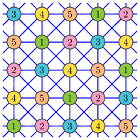
Figure 2: A proper 5-colouring of $C_{\_}5\boxtimes C_{\_}5$

By Lemma 10, for all graphs $G_{\_}1$ and $G_{\_}2$,

$$\raisebox{1.55pt}{\scalebox{1.2}{$\chi$}}^{f}(G_{\_}1\boxtimes G_{\_}2)\leqslant\raisebox{1.55pt}{\scalebox{1.2}{$\chi$}}^{f}(G_{\_}1)\raisebox{1.55pt}{\scalebox{1.2}{$\chi$}}^{f}(G_{\_}2),$$

with equality when $G_{\_}1$ or $G_{\_}2$ is a complete graph [41]. It is tempting therefore to hope for an analogous lower bound on $\raisebox{1.55pt}{\scalebox{1.2}{$\chi$}}^{f}(G_{\_}1\boxtimes G_{\_}2)$ in terms of $\raisebox{1.55pt}{\scalebox{1.2}{$\chi$}}^{f}(G_{\_}1)$ and $\raisebox{1.55pt}{\scalebox{1.2}{$\chi$}}^{f}(G_{\_}2)$ for all graphs $G_{\_}1$ and $G_{\_}2$. The following lemma dashes that hope.

Lemma 11.

For infinitely many $n\in\mathbb{N}$ there is an $n$-vertex graph $G$ such that

$$\raisebox{1.55pt}{\scalebox{1.2}{$\chi$}}^{f}(G\boxtimes G)\leqslant\frac{(256+o(1))\log^{4}n}{n}\,\raisebox{1.55pt}{\scalebox{1.2}{$\chi$}}^{f}(G)^{2}.$$

Proof.

Alon and Orlitsky [5, Theorems 5 and 6] proved that for infinitely many $n\in\mathbb{N}$, there is a (Cayley) graph $G$ on $n$ vertices with $\chi(G\boxtimes G)\leqslant n$ and $\alpha(G)\leqslant(16+o(1))\log^{2}n$. By Lemma 6,

$$\raisebox{1.55pt}{\scalebox{1.2}{$\chi$}}^{f}(G\boxtimes G)\leqslant\chi(G\boxtimes G)\leqslant n\leqslant\; \frac{(256+o(1))\log^{4}n}{n}\left(\frac{n}{\alpha(G)}\right)^{2}$$

$$\leqslant\; \frac{(256+o(1))\log^{4}n}{n}\,\raisebox{1.55pt}{\scalebox{1.2}{$\chi$}}^{f}(G)^{2}.\qed$$

The next lemma generalises Lemmas 9 and 10.

Lemma 12.

Let $G_{\_}1,\dots,G_{\_}d$ be graphs, such that $G_{\_}i$ is $(p_{\_}i\!:\!q_{\_}i)$-colourable with clustering $c_{\_}i$, for each $i\in[1,d]$. Then $G:=G_{\_}1\boxtimes\cdots\boxtimes G_{\_}d$ is $(\prod_{\_}ip_{\_}i:\prod_{\_}iq_{\_}i)$-colourable with clustering $\prod_{\_}ic_{\_}i$.

Proof.

For $i\in[1,d]$, let $\phi_{\_}i$ be a $(p_{\_}i\!:\!q_{\_}i)$-colouring of $G_{\_}i$ with clustering $c_{\_}i$. Let $\phi$ be the colouring of $G$, where each vertex $v=(v_{\_}1,\dots,v_{\_}d)$ of $G$ is coloured $\phi(v):=\{(a_{\_}1,\dots,a_{\_}d):a_{\_}i\in\phi_{\_}i(v_{\_}i),i\in[1,d]\}$. So each vertex of $G$ is assigned a set of $\prod_{\_}iq_{\_}i$ colours, and there are $\prod_{\_}ip_{\_}i$ colours in total. Let $X:=X_{\_}1\boxtimes\dots\boxtimes X_{\_}d$, where each $X_{\_}i$ is a monochromatic component of $G_{\_}i$ using colour $a_{\_}i$. Then $X$ is a monochromatic connected induced subgraph of $G$ using colour $(a_{\_}1,\dots,a_{\_}d)$. Consider any edge $(v_{\_}1,\dots,v_{\_}d)(w_{\_}1,\dots,w_{\_}d)$ of $G$ with $(v_{\_}1,\dots,v_{\_}d)\in V(X)$ and $(w_{\_}1,\dots,w_{\_}d)\not\in V(X)$. Thus $v_{\_}iw_{\_}i\in E(G_{\_}i)$ and $w_{\_}i\not\in V(X_{\_}i)$ for some $i\in\{1,\dots,d\}$. Hence $a_{\_}i\not\in\phi_{\_}i(w_{\_}i)$, implying $(a_{\_}1,\dots,a_{\_}d)\not\in\phi(w)$. Hence $X$ is a monochromatic component of $G$ using colour $(a_{\_}1,\dots,a_{\_}d)$. As $X$ contains at most $\prod_{\_}ic_{\_}i$ vertices, it follows that $\phi$ has clustering at most $\prod_{\_}ic_{\_}i$. ∎

Lemma 12 implies the following analogues of Lemma 9 for clustered colouring.

Theorem 13.

For all graph classes $\mathcal{G}_{\_}1,\dots,\mathcal{G}_{\_}d$

$$\raisebox{1.55pt}{\scalebox{1.2}{$\chi$}}_{\star}(\mathcal{G}_{\_}1\boxtimes\dots\boxtimes\mathcal{G}_{\_}d)\leqslant\prod_{\_}{i=1}^{d}\raisebox{1.55pt}{\scalebox{1.2}{$\chi$}}_{\star}(\mathcal{G}_{\_}i).$$

It is interesting to consider when the naive upper bound in Theorem 13 is tight. Theorem 16 below shows that this result is tight for products of closures of high-degree trees.

Finally, note that Lemma 12 implies the following basic observation.

Lemma 14.

If a graph $G$ is $k$-colourable with clustering $c$, then $G\boxtimes K_{\_}t$ is $k$-colourable with clustering $ct$.

More generally, Theorem 13 implies:

Lemma 15.

If a graph $G$ is $(p\!:\!q)$-colourable with clustering $c$, then $G\boxtimes K_{\_}t$ is $(p\!:\!q)$-colourable with clustering $ct$.

3 Products of Tree-Closures

This section presents examples of graphs that show that the naive upper bound in Theorem 13 is tight.

The depth of a node in a rooted tree is its distance to the root plus one. For $k,n\in\mathbb{N}$, let $T_{\_}{k,n}$ be the rooted tree in which every leaf is at depth $k$, and every non-leaf has $n$ children. Let $C_{\_}{k,n}$ be the graph obtained from $T_{\_}{k,n}$ by adding an edge between every ancestor and descendant (called the closure of $T_{\_}{k,n}$). Colouring each vertex by its distance from the root gives a $k$-colouring of $C_{\_}{k,n}$, and any root-leaf path in $C_{\_}{k,n}$ induces a $k$-clique. So $\chi(C_{\_}{k,n})=k$.

The class $\mathcal{C}_{\_}k:=\{C_{\_}{k,n}:n\in\mathbb{N}\}$ is important for defective and clustered colouring, and is often called the ‘standard’ example. It is well-known and easily proved (see [70]) that

$$\raisebox{1.55pt}{\scalebox{1.2}{$\chi$}}_{\Delta}(\mathcal{C}_{\_}k)=\raisebox{1.55pt}{\scalebox{1.2}{$\chi$}}_{\star}(\mathcal{C}_{\_}k)=\raisebox{1.55pt}{\scalebox{1.2}{$\chi$}}(\mathcal{C}_{\_}k)=k.$$

Norin et al. [58] extended this result (using a result of Dvořák and Sereni [20]) to the setting of defective and clustered fractional chromatic number by showing that

$$\raisebox{1.55pt}{\scalebox{1.2}{$\chi$}}^{f}_{\Delta}(\mathcal{C}_{\_}k)=\raisebox{1.55pt}{\scalebox{1.2}{$\chi$}}^{f}_{\star}(\mathcal{C}_{\_}k)=\raisebox{1.55pt}{\scalebox{1.2}{$\chi$}}^{f}(\mathcal{C}_{\_}k)=\raisebox{1.55pt}{\scalebox{1.2}{$\chi$}}_{\Delta}(\mathcal{C}_{\_}k)=\raisebox{1.55pt}{\scalebox{1.2}{$\chi$}}_{\star}(\mathcal{C}_{\_}k)=\raisebox{1.55pt}{\scalebox{1.2}{$\chi$}}(\mathcal{C}_{\_}k)=k.$$

Here we give an elementary and self-contained proof of this result. In fact, we prove the following generalisation in terms of strong products. This shows that Theorem 13 is tight, even for fractional colourings.

Theorem 16.

For all $k,d\in\mathbb{N}$, if $\mathcal{G}:=\boxtimes_{\_}d\mathcal{C}_{\_}{k}$ then

$$\raisebox{1.55pt}{\scalebox{1.2}{$\chi$}}^{f}_{\Delta}(\mathcal{G})=\raisebox{1.55pt}{\scalebox{1.2}{$\chi$}}^{f}_{\star}(\mathcal{G})=\raisebox{1.55pt}{\scalebox{1.2}{$\chi$}}^{f}(\mathcal{G})=\raisebox{1.55pt}{\scalebox{1.2}{$\chi$}}_{\Delta}(\mathcal{G})=\raisebox{1.55pt}{\scalebox{1.2}{$\chi$}}_{\star}(\mathcal{G})=\raisebox{1.55pt}{\scalebox{1.2}{$\chi$}}(\mathcal{G})=k^{d}.$$

Proof.

Let $K:=k^{d}$. It follows from the definitions that $\raisebox{1.55pt}{\scalebox{1.2}{$\chi$}}^{f}_{\Delta}(\mathcal{G})\leqslant\raisebox{1.55pt}{\scalebox{1.2}{$\chi$}}_{\Delta}(\mathcal{G})\leqslant\chi(\mathcal{G})=K$ and $\raisebox{1.55pt}{\scalebox{1.2}{$\chi$}}^{f}_{\Delta}(\mathcal{G})\leqslant\raisebox{1.55pt}{\scalebox{1.2}{$\chi$}}^{f}_{\star}(\mathcal{G})\leqslant\raisebox{1.55pt}{\scalebox{1.2}{$\chi$}}_{\star}(\mathcal{G})\leqslant\chi(\mathcal{G})=K$ and $\raisebox{1.55pt}{\scalebox{1.2}{$\chi$}}^{f}_{\Delta}(\mathcal{G})\leqslant\raisebox{1.55pt}{\scalebox{1.2}{$\chi$}}^{f}(\mathcal{G})\leqslant\chi(\mathcal{G})=K$. Thus it suffices to prove that $\raisebox{1.55pt}{\scalebox{1.2}{$\chi$}}^{f}_{\Delta}(\mathcal{G})\geqslant K$. Recall that $\raisebox{1.55pt}{\scalebox{1.2}{$\chi$}}^{f}_{\Delta}(\mathcal{G})$ is the infimum of all $t\in\mathbb{R}$ such that, for some $c\in\mathbb{N}$, for every $G\in\mathcal{G}$ there exists $p,q\in\mathbb{N}$ such that $p\leqslant tq$ and $G$ is $(p\!:\!q)$-colourable with defect $c$.

Suppose for the sake of contradiction that $\raisebox{1.55pt}{\scalebox{1.2}{$\chi$}}^{f}_{\Delta}(\mathcal{G})\leqslant K-\epsilon$, for some $\epsilon>0$. It follows that there exists $c\in\mathbb{N}$ such that for every integer $n$ there exist $p,q\in\mathbb{N}$ such that $p\leqslant(K-\epsilon)q$ and $\boxtimes_{\_}dC_{\_}{k,n}$ is $(p\!:\!q)$-colourable with defect $c$.

For $n\in\mathbb{N}$, consider the graph $G=\boxtimes_{\_}dC_{\_}{k,n}$ and a $(p\!:\!q)$-colouring of $G$ with defect $c$ such that $p\leqslant(K-\epsilon)q$. We will prove that for fixed $k$, $d$, and $\epsilon$, the value of $c$ must be at least linear in $n$. Since $n$ can be chosen to be arbitrary, this immediately yields the desired contradiction.

Each vertex $x$ of $G$ is a $d$-tuple $(x_{\_}1,\ldots,x_{\_}d)$, where each $x_{\_}i$ is a vertex of $C_{\_}{k,n}$. Whenever we mention ancestors, descendants, leaves and the depth of vertices in $C_{\_}{k,n}$, these terms refer to the corresponding notions in the spanning subgraph $T_{\_}{k,n}$ of $C_{\_}{k,n}$. Note that distinct vertices $x=(x_{\_}1,\ldots,x_{\_}d)$ and $y=(y_{\_}1,\ldots,y_{\_}d)$ are adjacent in $G$ if and only if for each $i\in[d]$, $x_{\_}i$ is an ancestor of $y_{\_}i$ or $y_{\_}i$ is an ancestor of $x_{\_}i$ in $C_{\_}{k,n}$ (where we adopt the convention that every vertex is an ancestor and descendant of itself).

For each $k$-tuple of non-negative integers $s=(s_{\_}1,\ldots,s_{\_}k)$ such that $\sum_{\_}{i=1}^{k}s_{\_}i=d$, define $V_{\_}s$ to be the set of vertices $x=(x_{\_}1,\ldots,x_{\_}d)$ of $G$ such that for each $i\in[k]$, there are precisely $s_{\_}i$ indices $j\in[d]$ such that $x_{\_}j$ has depth $i$ in $C_{\_}{k,n}$. Since $C_{\_}{k,n}$ contains $n^{i-1}$ vertices at depth $i$ (for each $i\in[d]$) and since $\binom{a}{b}\leqslant 2^{a}$,

$$|V_{\_}s|={d\choose s_{\_}1}{d-s_{\_}1\choose s_{\_}2}\cdots{d-s_{\_}1-\cdots-s_{\_}{k-1}\choose s_{\_}k}\cdot n^{s_{\_}2}n^{2s_{\_}3}\cdots n^{(k-1)s_{\_}k}\leqslant 2^{dk}\cdot n^{\sum_{\_}{i=1}^{k}(i-1)s_{\_}i}.$$

Let $V^{*}:=V_{\_}{(0,\ldots,0,d)}$; that is, $V^{*}$ is the set of vertices $x=(x_{\_}1,\ldots,x_{\_}d)$ of $G$ such that $x_{\_}1,\ldots,x_{\_}d$ are leaves of $C_{\_}{k,n}$. Note that $|V^{*}|=n^{d(k-1)}$.

For each vertex $x=(x_{\_}1,\ldots,x_{\_}d)\in V^{*}$, let $Q(x)$ be the set of vertices $y=(y_{\_}1,\ldots,y_{\_}d)$ of $G$ such that for each $i\in[d]$, $y_{\_}i$ is an ancestor of $x_{\_}i$ in $C_{\_}{k,n}$. By the definition of $G$, $Q(x)$ is a clique of size $k^{d}=K$ (including $x$). Let $S_{\_}1,\ldots,S_{\_}K$ be the sets of colours assigned to the elements of $Q(x)$ (so each $S_{\_}i$ is a $q$-element subset of $[p]$, with $p\leqslant(K-\epsilon)q$). We claim that there are indices $i<j$ such that $|S_{\_}i\cap S_{\_}j|\geqslant\tfrac{\epsilon}{K^{2}}\cdot q$. If not, for each $i\in[K]$, $S_{\_}i$ has at least $q-(i-1)\tfrac{\epsilon}{K^{2}}\cdot q$ elements not in $S_{\_}1,S_{\_}2,\ldots S_{\_}{i-1}$. Thus

$$|\bigcup_{\_}{i=1}^{K}S_{\_}i|\geqslant\sum_{\_}{i=1}^{K}(q-(i-1)\tfrac{\epsilon}{K^{2}}\cdot q)>Kq-\tfrac{K^{2}}{2}\cdot\tfrac{\epsilon}{K^{2}}\cdot q>(K-\epsilon)q\geqslant p,$$

which is a contradiction. Thus there exist distinct vertices $u,v\in Q(x)$ whose sets of colours intersect in at least $\tfrac{\epsilon}{K^{2}}\cdot q$ elements. Assume without loss of generality that $u\in V_{\_}{s}$ and $v\in V_{\_}t$, and the sequence $s$ precedes $t$ in lexicographic order. Orient the edge $uv$ from $u$ to $v$ and charge $x$ to the arc $(u,v)$.

We now bound the number of vertices $x=(x_{\_}1,\ldots,x_{\_}d)\in V^{*}$ that are charged to a given arc $(u,v)$, with $u=(u_{\_}1,\ldots,u_{\_}d)\in V_{\_}s$ and $v=(v_{\_}1\ldots,v_{\_}d)\in V_{\_}t$, where $s$ precedes $t=(t_{\_}1,\ldots,t_{\_}k)$ in lexicographic order. By definition, if $x$ is charged to $(u,v)$, each $x_{\_}i$ is a descendant of $u_{\_}i$ and $v_{\_}i$ (and in particular $u_{\_}i$ and $v_{\_}i$ are also in ancestor relationship). Each vertex at depth $i$ in $C_{\_}{k,n}$ has precisely $n^{k-i}$ descendants that are leaves in $C_{\_}{k,n}$. Thus (considering only $v_{\_}1,\dots,v_{\_}d$), at most

$$\prod_{\_}{i=1}^{k}n^{t_{\_}i(k-i)}=n^{\sum_{\_}{i=1}^{k}t_{\_}i(k-i)}$$

vertices of $V^{*}$ are charged to $(u,v)$.

We claim that there is an index $i\in[d]$, such that $u_{\_}i$ is a strict descendant of $v_{\_}i$. Since $x_{\_}i$ is a descendant of $u_{\_}i$, it follows that the bound above can be divided by a factor $n$, and thus at most $n^{-1+\sum_{\_}{i=1}^{k}t_{\_}i(k-i)}$ vertices of $V^{*}$ are charged to $(u,v)$. To prove the claim, consider first the $t_{\_}1$ indices $i\in[d]$ such that $v_{\_}i$ has depth 1. If $u_{\_}i$ has depth greater than 1 for one of these indices, then the desired property holds. So we may assume that all the corresponding $u_{\_}i$’s also have depth 1. Since $s$ precedes $t$ in lexicographic order, $s_{\_}1\leqslant t_{\_}1$ and thus $s_{\_}1=t_{\_}1$. It follows that for each $i\in[d]$, $u_{\_}i$ has depth 1 if and only if $v_{\_}i$ has depth 1. By considering the $t_{\_}2$ indices $i$ such that $v_{\_}i$ has depth 2, the same reasoning shows that for each $i\in[d]$, $v_{\_}i$ has depth 2 if and only if $u_{\_}i$ has depth 2. By iterating this argument, for each $i\in[d]$ and $j\in[k]$, $v_{\_}i$ has depth $j$ if and only if $u_{\_}i$ has depth $j$. Since $u_{\_}i$ and $v_{\_}i$ are ancestors for each $i\in[d]$, we have that $u=v$, which is a contradiction. It follows that some $u_{\_}i$ is a strict ancestor of $v_{\_}i$, and thus (as argued above) at most $n^{-1+\sum_{\_}{i=1}^{k}t_{\_}i(k-i)}$ vertices of $V^{*}$ are charged to $(u,v)$.

Each vertex of $V^{*}$ is charged to some arc $(u,v)$, where $u$ and $v$ share at least $\tfrac{\epsilon}{K^{2}}\cdot q$ colours. We claim that for each $v\in V^{*}$, there are at most $cK^{2}/\epsilon$ such arcs $(u,v)$. If not, the $q$ colours of $v$ must appear (with repetition) more than $\tfrac{\epsilon}{K^{2}}\cdot q\cdot cK^{2}/\epsilon=cq$ times in the neighbourhood of $v$. By the pigeonhole principle some colour of $v$ appears more than $c$ times in the neighbourhood of $v$, which contradicts the assumption that the colouring has defect at most $c$.

For each vertex $v\in V_{\_}t$, where $t=(t_{\_}1,\ldots,t_{\_}k)$, and for each of the at most $cK^{2}/\epsilon$ arcs $(u,v)$ as above, we have proved that at most $n^{-1+\sum_{\_}{i=1}^{k}t_{\_}i(k-i)}$ vertices of $V^{*}$ are charged to $(u,v)$. Since $|V_{\_}t|\leqslant 2^{dk}\cdot n^{\sum_{\_}{i=1}^{k}(i-1)t_{\_}i}$ and $\sum_{\_}{i=1}^{k}t_{\_}i=d$, at most

$$c\tfrac{K^{2}}{\epsilon}\cdot 2^{dk}\cdot n^{\sum_{\_}{i=1}^{k}(i-1)t_{\_}i}\cdot n^{-1+\sum_{\_}{i=1}^{k}t_{\_}i(k-i)}=c\tfrac{K^{2}}{\epsilon}\cdot 2^{dk}\cdot n^{-1+\sum_{\_}{i=1}^{k}(k-1)t_{\_}i}=c\tfrac{K^{2}}{\epsilon}\cdot 2^{dk}\cdot n^{d(k-1)-1}$$

vertices of $V^{*}$ are charged to an arc $(u,v)$. Since there are at most $(d+1)^{k}$ possible $k$-tuples of integers $t=(t_{\_}1,\ldots,t_{\_}k)$ with $\sum_{\_}{i=1}^{k}t_{\_}i=d$, it follows that

$$n^{d(k-1)}=|V^{*}|\leqslant(d+1)^{k}c\cdot\tfrac{K^{2}}{\epsilon}\cdot 2^{dk}\cdot n^{d(k-1)-1},$$

and thus $c\geqslant n\cdot\tfrac{\epsilon}{k^{2d}(d+1)^{k}2^{dk}}$, as desired. ∎

Let $\mathcal{S}$ be the class of all star graphs; that is, $\mathcal{S}:=\{K_{\_}{1,n}:n\in\mathbb{N}\}$. Since $K_{\_}{1,n}\cong C_{\_}{2,n}$, Theorem 16 implies:

Corollary 17.

For $d\in\mathbb{N}$, let $\mathcal{S}^{d}$ be the class of all $d$-dimensional strong products of star graphs. Then

$$\raisebox{1.55pt}{\scalebox{1.2}{$\chi$}}^{f}_{\Delta}(\mathcal{S}^{d})=\raisebox{1.55pt}{\scalebox{1.2}{$\chi$}}^{f}_{\star}(\mathcal{S}^{d})=\raisebox{1.55pt}{\scalebox{1.2}{$\chi$}}^{f}(\mathcal{S}^{d})=\raisebox{1.55pt}{\scalebox{1.2}{$\chi$}}_{\Delta}(\mathcal{S}^{d})=\raisebox{1.55pt}{\scalebox{1.2}{$\chi$}}_{\star}(\mathcal{S}^{d})=\raisebox{1.55pt}{\scalebox{1.2}{$\chi$}}(\mathcal{S}^{d})=2^{d}.$$

4 Consistent colourings

A $(p\!:\!q)$-colouring $\alpha$ of a graph $G$ is consistent if for each vertex $x\in V(G)$, there is an ordering $\alpha_{\_}x^{1},\dots,\alpha_{\_}x^{q}$ of $\alpha(x)$, such that $\alpha_{\_}x^{i}\neq\alpha_{\_}y^{j}$ for each edge $xy\in E(G)$ and for all distinct $i,j\in[1,q]$. For example, the following $(4\!:\!3)$-colouring of a path is consistent:

$$\begin{array}[]{c}0\\ 1\\ 2\end{array},\begin{array}[]{c}0\\ 1\\ 3\end{array},\begin{array}[]{c}0\\ 2\\ 3\end{array},\begin{array}[]{c}1\\ 2\\ 3\end{array},\begin{array}[]{c}1\\ 2\\ 0\end{array},\begin{array}[]{c}1\\ 3\\ 0\end{array},\begin{array}[]{c}2\\ 3\\ 0\end{array},\begin{array}[]{c}2\\ 3\\ 1\end{array},\begin{array}[]{c}2\\ 0\\ 1\end{array},\begin{array}[]{c}3\\ 0\\ 1\end{array},\begin{array}[]{c}3\\ 0\\ 2\end{array},\begin{array}[]{c}3\\ 1\\ 2\end{array},\begin{array}[]{c}0\\ 1\\ 2\end{array},\dots$$

Lemma 18.

If a graph $G$ has a consistent $(p\!:\!q)$-colouring with clustering $c_{\_}1$, and a graph $H$ has a $(q\!:\!r)$-colouring with clustering $c_{\_}2$, then $G\boxtimes H$ has a $(p\!:\!r)$-colouring with clustering $c_{\_}1c_{\_}2$.

Proof.

Let $\alpha$ be a consistent $(p\!:\!q)$-colouring of $G$ with clustering $c_{\_}1$, that is each vertex $x\in V(G)$ has colours $\alpha^{1}_{\_}x,\ldots,\alpha^{q}_{\_}x$ such that $\alpha_{\_}x^{i}\neq\alpha_{\_}y^{j}$ for each edge $xy\in E(G)$ and for all distinct $i,j\in[1,q]$. Let $\beta$ be a $(q\!:\!r)$-colouring of $H$ with clustering $c_{\_}2$, with colours from $[q]$. Colour each vertex $(x,v)$ of $G\boxtimes H$ by $\{\alpha_{\_}x^{i}:i\in\beta(v)\}\in\binom{[p]}{r}$.

Let $Z$ be a monochromatic component of $G\boxtimes H$ defined by colour $c\in[p]$. Let $(x,v)$ be any vertex in $Z$. So $c=\alpha_{\_}x^{i}$ for some $i\in\beta(v)$. Let $A_{\_}x$ be the $\alpha$-component of $G$ defined by $c$ and containing $x$. Let $B_{\_}v$ be the $\beta$-component of $H$ defined by $i$ and containing $v$.

Consider an edge $(x,v)(y,w)$ of $Z$. Thus $c=\alpha_{\_}y^{j}$ for some $j\in\beta(w)$. Since $A_{\_}x$ is an $\alpha$-component containing $x$ and ($xy\in E(G)$ or $x=y$), the vertex $y$ is also in $A_{\_}x$. If $xy\in E(G)$, then $i=j$ since $\alpha$ is consistent. Otherwise, $x=y$ and $\alpha_{\_}x^{i}=c=\alpha_{\_}y^{j}=\alpha_{\_}x^{j}$, again implying $i=j$. In both cases $i=j\in\beta(w)$. Since $B_{\_}v$ is a $\beta$-component defined by $i$ and containing $v$ and ($vw\in E(G)$ or $v=w$), the vertex $w$ is also in $B_{\_}v$.

For every edge $(x,v)(y,w)$ of $Z$, we have shown that $y\in V(A_{\_}x)$ and $w\in V(B_{\_}v)$. Thus $A_{\_}y=A_{\_}x$ and $B_{\_}w=B_{\_}v$. Since $Z$ is connected, for all vertices $(x,v)$ and $(y,w)$ of $Z$, we have $A_{\_}x=A_{\_}y$ and $B_{\_}v=B_{\_}w$. Hence $Z\subseteq A_{\_}x\boxtimes B_{\_}v$ for any $(x,v)\in V(Z)$.

Since $A_{\_}x$ is $\alpha$-monochromatic, $|A_{\_}x|\leqslant c_{\_}1$. Since $B_{\_}v$ is $\beta$-monochromatic, $|B_{\_}v|\leqslant c_{\_}2$. As $Z\subseteq A_{\_}x\boxtimes B_{\_}v$, $|Z|\leqslant|A_{\_}x\boxtimes B_{\_}v|\leqslant c_{\_}1c_{\_}2$. Hence, our colouring of $G\boxtimes H$ has clustering $c_{\_}1c_{\_}2$. ∎

Every proper colouring is consistent, so Lemma 18 implies:

Corollary 19.

If a graph $G$ has a proper $(p\!:\!q)$-colouring, and a graph $H$ has a $(q\!:\!r)$-colouring with clustering $c$, then $G\boxtimes H$ has a $(p\!:\!r)$-colouring with clustering $c$.

Corollary 20.

If a graph $G$ has a proper $(p\!:\!q)$-colouring and a graph $H$ has a proper $(q\!:\!r)$-colouring, then $G\boxtimes H$ has a proper $(p\!:\!r)$-colouring.

Lemma 12 states that a $(p_{\_}1\!:\!q_{\_}1)$-colouring of a graph $G$ (with bounded clustering) can be combined with a $(p_{\_}2\!:\!q_{\_}2)$-colouring of a graph $H$ (with bounded clustering) to produce a $(p_{\_}1p_{\_}2\!:\!q_{\_}1q_{\_}2)$-colouring of $G\boxtimes H$ (with bounded clustering). A natural question is whether this fractional colouring can be simplified; that is, is there a $(p_{\_}3\!:\!q_{\_}3)$-colouring of $G\boxtimes H$ with $\tfrac{p_{\_}3}{q_{\_}3}\leqslant\tfrac{p_{\_}1p_{\_}2}{q_{\_}1q_{\_}2}$ and $p_{\_}3<p_{\_}1p_{\_}2$? There is no hope to obtain such a simplification in general, since if $G$ and $H$ are complete graphs and $q_{\_}1=q_{\_}2=1$, then $G\boxtimes H$ is a complete graph on $p_{\_}1p_{\_}2$ vertices. However, Corollary 19 shows that when the fractional colouring of $G$ is proper and $q_{\_}1=p_{\_}2$, the resulting fractional colouring of $G\boxtimes H$ can be simplified significantly.

We now show another way to simplify the $(p_{\_}1p_{\_}2\!:\!q_{\_}1q_{\_}2)$-colouring of the graph $G\boxtimes H$, by allowing a small loss on the fraction $\tfrac{p_{\_}1p_{\_}2}{q_{\_}1q_{\_}2}$. Below we only consider the case $p_{\_}1=p_{\_}2$ and $q_{\_}1=q_{\_}2$ for simplicity, but the technique can be extended to the more general case. We use the Chernoff bound: For any $0\leqslant t\leqslant nx$, the probability that the binomial distribution $\mathrm{Bin}(n,x)$ with parameters $n$ and $x$ differs from its expectation $nx$ by at least $t$ satisfies

$$\,\mathbb{P}(|\mathrm{Bin}(n,x)-nx|>t)<2\exp(-t^{2}/(3nx)).$$

Lemma 21.

Assume that $G$ has a $(p\!:\!q)$-colouring (with bounded clustering) and $H$ has a $(p\!:\!q)$-colouring (with bounded clustering). Then for any real number $0<x\leqslant 1$, $G\boxtimes H$ has a $\Big{(}xp^{2}+O(p\sqrt{x}):\big{(}xq^{2}-O(q^{3/2}\sqrt{x\log p})\big{)}\Big{)}$-colouring (with bounded clustering).

Proof.

Let $X$ be a random subset of $[p]^{2}$ obtained by including each element of $[p]^{2}$ independently with probability $x$. By the Chernoff bound, $p^{\prime}:=|X|\leqslant xp^{2}+O(p\sqrt{x})$ with high probability (i.e., with probability tending to $1$ as $p\to\infty$).

Consider two $q$-element subsets $S,T\subseteq[p]$. Then it follows from the Chernoff bound that for any $0\leqslant t\leqslant xq^{2}$, the probability that $S\times T$ contains less than $xq^{2}-t$ elements of $X$ is at most $2\exp(-t^{2}/(3q^{2}x))$. By the union bound, the probability that there exist two $q$-element subsets $S,T\subseteq[p]$ with $|(S\times T)\cap X|<xq^{2}-t$ is at most $p^{q}\cdot p^{q}\cdot 2\exp(-t^{2}/(3q^{2}x))<2\exp(2q\log p-t^{2}/(3q^{2}x))$. By taking $t=\Theta(q^{3/2}\sqrt{x\log p})$, this quantity is less than $\tfrac{1}{2}$.

It follows that there exists a subset $X\subseteq[p]^{2}$ of at most $p^{\prime}=xp^{2}+O(p\sqrt{x})$ elements, such that for all $q$-elements subsets $S,T\subseteq[p]$, $|(S\times T)\cap X|\geqslant q^{\prime}:=xq^{2}-O(q^{3/2}\sqrt{x\log p})$.

Let $c_{\_}G$ be a $(p\!:\!q)$-colouring of $G$ with colours $[p]$ and let $c_{\_}H$ be a $(p\!:\!q)$-colouring of $H$ with colours $[p]$. For any pair $(i,j)\in X$ define the colour class $C_{\_}{ij}=\{u\in V(G)\,:\,i\in c_{\_}G(u)\}\times\{v\in V(H)\,:\,j\in c_{\_}H(v)\}$ in $G\boxtimes H$.

Let $c$ denote the resulting colouring of $G\boxtimes H$, and observe that if $c_{\_}G$ and $c_{\_}H$ are proper, so is $c$, and if $c_{\_}G$ and $c_{\_}H$ have bounded clustering, so does $c$, since each colour class in $c$ is the cartesian product of a colour class of $G$ and a colour class of $H$. Moreover $c$ uses at most $p^{\prime}$ colours, and each vertex of $G\boxtimes H$ receives at least $q^{\prime}$ colours. It follows that $c$ is a $(p^{\prime}\!:\!q^{\prime})$-colouring of $G\boxtimes H$ (with bounded clustering), as desired. ∎

4.1 Paths and Cycles

The next lemma shows how to obtain a consistent colouring of a tree with small clustering.

Lemma 22.

If a tree $T$ has an edge-partition $E_{\_}1,\dots,E_{\_}k$ such that for each $i\in[1,k]$ each component of $T-E_{\_}i$ has at most $c$ vertices, then $T$ has a consistent $(k+1\!:\!k)$-colouring with clustering $c$.

Proof.

Root $T$ at some leaf vertex $r$ and orient $T$ away from $r$. We now label each vertex $v$ of $T$ by a sequence $(\ell^{1}_{\_}v,\dots,\ell^{k}_{\_}v)$ of distinct elements of $\{1,\dots,k+1\}$. First label $r$ by $(1,\dots,k)$. Now label vertices in order of non-decreasing distance from $r$. Consider an arc $vw$ with $v$ labelled $(\ell^{1}_{\_}v,\dots,\ell^{k}_{\_}v)$ and $w$ unlabelled. Say $vw\in E_{\_}i$. Let $z$ be the element of $\{1,\dots,k+1\}\setminus\{\ell^{1}_{\_}v,\dots,\ell^{k}_{\_}v\}$. Then label $w$ by $(\ell^{1}_{\_}v,\dots,\ell^{i-1}_{\_}v,z,\ell^{i+1}_{\_}v,\dots,\ell^{k}_{\_}v)$. Label every vertex in $T$ by repeated application of this rule. It is immediate that this labelling determines a consistent $(k+1\!:\!k)$-colouring of $T$.

Consider a monochromatic component $X$ of $T$ determined by colour $i$. If $vw$ is an edge of $T$ with $v\in V(X)$ and $w\not\in V(X)$ and $vw\in E_{\_}j$, then $\ell_{\_}j(v)=i$ and $\ell_{\_}j(w)\neq i$ and the only colour not assigned to $w$ is $\ell_{\_}j(v)=i$. By consistency, $\ell_{\_}j(x)=i$ for every $x\in V(X)$, and for every edge $xy\in E(T)$ with $x\in V(X)$ and $y\not\in V(X)$ we have $xy\in E_{\_}j$. Thus $X$ is contained in $T-E_{\_}j$ and has at most $c$ vertices. ∎

Lemma 23.

For every $k\in\mathbb{N}$, every path has a consistent $(k+1\!:\!k)$-colouring with clustering $k$.

Proof.

Let $e_{\_}1,\dots,e_{\_}n$ be the sequence of edges in a path $P$. For $i\in[0,k-1]$ let $E_{\_}i:=\{e_{\_}j:j\equiv i\pmod{k}\}$. So $E_{\_}0,\dots,E_{\_}{k-1}$ is an edge-partition of $P$ such that for each $i\in[0,k-1]$ each component of $T-E_{\_}i$ has at most $k$ vertices. By Lemma 22, $P$ has a consistent $(k+1\!:\!k)$ colouring with clustering $k$. ∎

Lemmas 23 and 18 imply the following result. Products with paths are of particular interest because of the results in Section 1.2.

Theorem 24.

If a graph $G$ is $k$-colourable with clustering $c$ and $P$ is a path, then $G\boxtimes P$ is $(k+1)$-colourable with clustering $ck$.

Recall that $\boxtimes_{\_}dP_{\_}{n}$ denotes the $d$-dimensional grid $P_{\_}n\boxtimes\cdots\boxtimes P_{\_}n$. Theorem 24 implies the upper bound in the following result. As discussed in Section 1.3, the lower bound comes from the $d$-dimensional Hex Lemma [27, 45, 54, 7, 54, 53, 37].

Corollary 25.

$\boxtimes_{\_}dP_{\_}{n}$ is $(d+1)$-colourable with clustering $d!$. Conversely, every $d$-colouring of $\boxtimes_{\_}dP_{\_}{n}$ has a monochromatic component of size at least $n$. Hence

$$\raisebox{1.55pt}{\scalebox{1.2}{$\chi$}}_{\star}(\{\boxtimes_{\_}dP_{\_}{n}:n\in\mathbb{N}\})=d+1.$$

Note that the corollary above can also be deduced from the following simple lemma, which does not use consistent colourings (however we need this notion to prove the stronger Theorem 24 above, and its generalisation Lemma 32 in Section 4.2).

Lemma 26.

If $G$ is $(p\!:\!q)$-colourable with clustering $c_{\_}1$ and $H$ is $(p\!:\!r)$-colourable with clustering $c_{\_}2$, and $q+r>p$, then $G\boxtimes H$ is $(p\!:\!(q+r-p))$-colourable with clustering $c_{\_}1c_{\_}2$.

Proof.

Consider a $(p\!:\!q)$-colouring of $G$ and a $(p\!:\!r)$-colouring of $H$ and for each $i\in[p]$, let the colour class of colour $i$ in $G\boxtimes H$ be the product of the colour class of colour $i$ in $G$ and the colour class of colour $i$ in $H$. Clearly, monochromatic components in $G\boxtimes H$ have size at most $c_{\_}1c_{\_}2$. Moreover, a pigeonhole argument tells us that each vertex of $G\boxtimes H$ is covered by at least $q+r-p$ colours in $G\boxtimes H$, as desired. ∎

In particular Lemma 26 shows that if $G$ is $(p\!:\!q)$-colourable with clustering $c$, and $P$ is a path, then $G\boxtimes P$ is $(p\!:\!q-1)$-colourable with clustering $(p-1)c$. Here we have used the statement of Lemma 23, that every path has a $(p\!:\!p-1)$-colouring with clustering $p-1$ (but we did not use the additional property that such a colouring could be taken to be consistent). By induction this easily implies Corollary 25.

It is an interesting open problem to determine the minimum clustering function in a $(d+1)$-colouring of $\boxtimes_{\_}dP_{\_}{n}$. Since $\boxtimes_{\_}dP_{\_}{n}$ contains a $2^{d}$-clique, every $(d+1)$-colouring has a monochromatic component with at least $2^{d}/(d+1)$ vertices.

The fractional clustered chromatic number of Hex grid graphs is very different from the clustered chromatic number.

Proposition 27.

For fixed $d\in\mathbb{N}$,

$$\raisebox{1.55pt}{\scalebox{1.2}{$\chi$}}^{f}_{\star}(\{\boxtimes_{\_}dP_{\_}{n}:n\in\mathbb{N}\})=1.$$

Proof.

Fix $\epsilon\in(0,1)$ and let $k:=\lceil 2d/\epsilon\rceil$. By Lemma 23, every path has a $(k+1\!:\!k)$-colouring with clustering $k$. By Lemma 12, for every $n\in\mathbb{N}$, the graph $\boxtimes_{\_}dP_{\_}n$ is $((k+1)^{d}\!:\!k^{d})$-colourable with clustering $k^{d}$. For $k\geqslant 2d$, it is easily proved by induction on $d$ that $(k+1)^{d}/k^{d}\leqslant 1+2d/k$. Thus $(k+1)^{d}/k^{d}\leqslant 1+\epsilon$. This says that for any $\epsilon>0$ there exists $c$ (namely, $\lceil 2d/\epsilon\rceil^{d}$) such that for every $n\in\mathbb{N}$, the graph $\boxtimes_{\_}dP_{\_}n$ is fractionally $(1+\epsilon)$-colourable with clustering $c$. The result follows. ∎

Proposition 27 can also be deduced from a result of Dvořák [18] (who proved that the conclusion holds for any class of bounded degree having sublinear separators). It can also be deduced from a result of Brodskiy et al. [9], which states that classes of bounded asymptotic dimension have fractional asymptotic dimension 1 (combined with the discussion of Section 1.4 on the connection between asymptotic dimension and clustered colouring for classes of graphs of bounded degree). Note that the main result of [9], which states that if $\mathcal{F}_{\_}1$ and $\mathcal{F}_{\_}2$ have asymptotic dimension $m_{\_}1$ and $m_{\_}2$, respectively, then $\mathcal{F}_{\_}1\boxtimes\mathcal{F}_{\_}2$ has asymptotic dimension $m_{\_}1+m_{\_}2$, is obtained by combining the result on fractional asymptotic dimension mentioned above with an elaborate version of Lemma 26.

Lemma 28.

For every $k\in\mathbb{N}$, every cycle has a consistent $(k+1\!:\!k)$-colouring with clustering $k^{2}+3k-1$.

Proof.

Let $C=(v_{\_}1,\dots,v_{\_}n)$ be an $n$-vertex cycle. Consider integers $a$ and $b\in[0,k(k+1)-1]$ such that $n=ak(k+1)+b$. By Lemma 23, the path $(v_{\_}1,\dots,v_{\_}{n-b})$ has a consistent $(k+1\!:\!k)$-colouring with clustering $k$. Observe that the colour sequences assigned to vertices repeat every $k(k+1)$ vertices. Thus $v_{\_}1$ and $v_{\_}{n-b}$ are assigned the same sequence of $k$ colours. Give this colour sequence to all of $v_{\_}{n-b+1},\dots,v_{\_}n$. We obtain a consistent $(k+1\!:\!k)$-colouring of $C$ with clustering $k+k(k+1)-1+k=k^{2}+3k-1$. ∎

Lemmas 23 and 28 imply that for every $\epsilon>0$ there exists $c\in\mathbb{N}$, such that every graph with maximum degree 2 is fractionally $(1+\epsilon)$-colourable with clustering $c$. Thus the fractional clustered chromatic number of graphs with maximum degree 2 equals 1. The following open problem naturally arises:

Question 29.

What is the fractional clustered chromatic number of graphs with maximum degree $\Delta$?

We now show that the same lower bound from the non-fractional setting (see [70]) holds in the fractional setting.

Proposition 30.

For every even integer $\Delta$, the fractional clustered chromatic number of the class of graphs with maximum degree $\Delta$ is at least $\frac{\Delta}{4}+\tfrac{1}{2}$.

Proof.

We need to prove that for any even integer $\Delta$ and any integer $c$, there is a graph $G$ of maximum degree $\Delta$ such that for any integers $p,q$, if $G$ is $(p\!:\!q)$-colourable with clustering $c$, then $\tfrac{p}{q}\geqslant\frac{\Delta}{4}+\tfrac{1}{2}$.

Fix an even integer $\Delta$ and an integer $c$, and consider a $(\frac{\Delta}{2}+1)$-regular graph $H$ with girth greater than $c$ (such a graph exists, as proved by Erdős and Sachs [22]). Let $G=L(H)$ be the line-graph of $H$. Note that $G$ is $\Delta$-regular. Let $p,q$ be such that $G$ is $(p\!:\!q)$-colourable with clustering $c$, and let $f$ be such a colouring. Consider an $f$-monochromatic subgraph of $G$ with vertex set $X$, so every component of $G[X]$ has at most $c$ vertices. Let $F_{\_}X$ be the set of edges of $H$ corresponding to the vertices of $X$ in $G$.

Since $H$ has girth greater than $c$, the subgraph of $H$ determined by the edges of $F$ is a forest, and thus $|X|=|F_{\_}X|<|V(H)|$. There are $p$ such monochromatic subgraphs and each vertex of $G$ is in exactly $q$ such subgraphs. Thus

$$q\tfrac{1}{2}(\tfrac{\Delta}{2}+1)|V(H)|=q|E(H)|=q|V(G)|=\sum_{\_}X|X|=\sum_{\_}{X}|F_{\_}X|<p|V(H)|.$$

Hence $\frac{p}{q}>\frac{\Delta}{4}+\tfrac{1}{2}$, as desired. ∎

The $\Delta=3$ case of Question 29 is an interesting problem. The line graph of the 1-subdivision of a high girth cubic graph provides a lower bound of $\frac{6}{5}$ on the fractional clustered chromatic number.

4.2 Trees and Treewidth

Lemma 23 is generalised for bounded degree trees as follows:

Lemma 31.

For all $k,\Delta\in\mathbb{N}$, every tree $T$ with maximum degree $\Delta\geqslant 3$ has a consistent $(k+1\!:\!k)$-colouring with clustering less than $2(\Delta-1)^{k-1}$.

Proof.

If $k=1$ then a proper 2-colouring of $T$ suffices. Now assume that $k\geqslant 2$. Root $T$ at some leaf vertex $r$. Consider the edge-partition $E_{\_}0,\dots,E_{\_}{k-1}$ of $T$, where $E_{\_}i$ is the set of edges $uv$ in $T$ such that $u$ is the parent of $v$ and $\operatorname{dist}_{\_}T(r,u)\equiv i\pmod{k}$. Each component $X$ of $T-E_{\_}i$ has height at most $k-1$ and each vertex $v$ in $X$ has at most $\Delta-1$ children in $X$, implying $|V(X)|\leqslant 1+(\Delta-1)+(\Delta-1)^{2}+\dots+(\Delta-1)^{k-1}=\frac{(\Delta-1)^{k}-1}{\Delta-2}<2(\Delta-1)^{k-1}$. The result then follows from Lemma 22. ∎

Lemmas 18 and 31 imply the following generalisation of Theorem 24:

Lemma 32.

If a graph $G$ is $k$-colourable with clustering $c$ and $T$ is a tree with maximum degree $\Delta\geqslant 3$, then $G\boxtimes T$ is $(k+1)$-colourable with clustering less than $2c(\Delta-1)^{k-1}$.

Lemma 32 leads to the next result. We emphasise that $T_{\_}1$ may have arbitrarily large maximum degree (if $T_{\_}1$ also has bounded degree then the result is again a simple consequence of Lemma 26, which does not use consistent colourings).

Theorem 33.

If $T_{\_}1,\dots,T_{\_}d$ are trees, such that each of $T_{\_}2,\dots,T_{\_}d$ have maximum degree at most $\Delta\geqslant 3$, then $T_{\_}1\boxtimes\dots\boxtimes T_{\_}d$ is $(d+1)$-colourable with clustering less than $2^{d}(\Delta-1)^{\binom{d}{2}}$.

Proof.

We proceed by induction on $d\geqslant 1$. In the base case, $T_{\_}1$ is 2-colourable with clustering 1. Now assume that $T_{\_}1\boxtimes\dots\boxtimes T_{\_}{d-1}$ is $d$-colourable with clustering less than $2^{d-1}(\Delta-1)^{\binom{d-1}{2}}$. Lemma 32 with $G=T_{\_}1\boxtimes\dots\boxtimes T_{\_}{d-1}$ implies that $T_{\_}1\boxtimes\dots\boxtimes T_{\_}{d}$ is $(d+1)$-colourable with clustering less than $2\cdot 2^{d-1}(\Delta-1)^{\binom{d-1}{2}}(\Delta-1)^{d-1}=2^{d}(\Delta-1)^{\binom{d}{2}}$. ∎

Theorem 33 is in sharp contrast with Corollary 17: for the strong product of $d$ stars we need $2^{d}$ colours even for defective colouring, whereas for bounded degree trees we only need $d+1$ colours in the stronger setting of clustered colouring. This highlights the power of assuming bounded degree in the above results.

Let $\mathcal{T}_{\_}k$ be the class of graphs with treewidth $k$. Such graphs are $k$-degenerate and $(k+1)$-colourable. Since the graph $C_{\_}{n,k}$ (defined in Section 3) has treewidth $k-1$, Theorem 16 implies that

$$\raisebox{1.55pt}{\scalebox{1.2}{$\chi$}}^{f}_{\Delta}(\mathcal{T}_{\_}k)=\raisebox{1.55pt}{\scalebox{1.2}{$\chi$}}^{f}_{\star}(\mathcal{T}_{\_}k)=\raisebox{1.55pt}{\scalebox{1.2}{$\chi$}}^{f}(\mathcal{T}_{\_}k)=\raisebox{1.55pt}{\scalebox{1.2}{$\chi$}}_{\Delta}(\mathcal{T}_{\_}k)=\raisebox{1.55pt}{\scalebox{1.2}{$\chi$}}_{\star}(\mathcal{T}_{\_}k)=\raisebox{1.55pt}{\scalebox{1.2}{$\chi$}}(\mathcal{T}_{\_}k)=k+1.$$

Alon et al. [3] showed that graphs of bounded treewidth and bounded degree are 2-colourable with bounded clustering. Note that Theorem 4 in Section 1.4 generalises this result ($d=1$) and generalises Theorem 33 ($k=1$). We now give a short proof of Theorem 4 (which we restate below for convenience) that does not use asymptotic dimension, or any results related to it.

See 4

Proof.

By Theorem 2, $G_{\_}i$ is a subgraph of $T_{\_}i\boxtimes K_{\_}{20k\Delta}$ for some tree $T_{\_}i$ with maximum degree at most $20k\Delta^{2}$. Thus $G_{\_}1\boxtimes\dots\boxtimes G_{\_}d$ is a subgraph of $(T_{\_}1\boxtimes K_{\_}{20k\Delta})\boxtimes\dots\boxtimes(T_{\_}d\boxtimes K_{\_}{20k\Delta})$, which is a subgraph of $(T_{\_}1\boxtimes\dots\boxtimes T_{\_}d)\boxtimes K_{\_}t$, where $t:=(20k\Delta)^{d}$. By Theorem 33, $T_{\_}1\boxtimes\dots\boxtimes T_{\_}d$ is $(d+1)$-colourable with clustering at most some function $c^{\prime}(d,k,\Delta)$. By Lemma 14, $(T_{\_}1\boxtimes\dots\boxtimes T_{\_}d)\boxtimes K_{\_}t$ and thus $G_{\_}1\boxtimes\dots\boxtimes G_{\_}d$ is $(d+1)$-colourable with clustering $c(d,k,\Delta):=c^{\prime}(d,k,\Delta)\cdot t$. ∎

The next result shows that for any sequence of non-trivial classes $\mathcal{G}_{\_}1,\dots,\mathcal{G}_{\_}d$, the bound on the number of colours in Theorem 4 is best possible.

Theorem 34.

If $\mathcal{G}_{\_}1,\dots,\mathcal{G}_{\_}d$ are graph classes with $\raisebox{1.55pt}{\scalebox{1.2}{$\chi$}}_{\star}(\mathcal{G}_{\_}i)\geqslant 2$ for each $i\in\{1,\dots,d\}$, then $\raisebox{1.55pt}{\scalebox{1.2}{$\chi$}}_{\star}(\mathcal{G}_{\_}1\boxtimes\dots\boxtimes\mathcal{G}_{\_}d)\geqslant d+1$.

Proof.

By replacing each class $\mathcal{G}_{\_}i$ by its monotone closure if necessary, we can assume without loss of generality that each class $\mathcal{G}_{\_}i$ is monotone (i.e., closed under taking subgraphs). If there is a constant $d$ such that every component of a graph of $\mathcal{G}_{\_}i$ has maximum degree at most $d$ and diameter at most $d$, then $\raisebox{1.55pt}{\scalebox{1.2}{$\chi$}}_{\star}(\mathcal{G}_{\_}i)\leqslant 1$. It follows that for any $1\leqslant i\leqslant d$, the graphs of the class $\mathcal{G}_{\_}i$ contain arbitrarily large degree vertices or arbitrarily long paths. By monotonicity, it follows that for some constant $1\leqslant k\leqslant d$, $\mathcal{G}_{\_}1\boxtimes\dots\boxtimes\mathcal{G}_{\_}d$ contains the class $(\boxtimes_{\_}k\mathcal{P})\boxtimes(\boxtimes_{\_}{d-k}\mathcal{S})$, where $\mathcal{P}$ denotes the class of all paths, and $\mathcal{S}$ denotes the class of all stars.

We claim that for any graph $G$, $\raisebox{1.55pt}{\scalebox{1.2}{$\chi$}}_{\star}(G\boxtimes\mathcal{P})\leqslant\raisebox{1.55pt}{\scalebox{1.2}{$\chi$}}_{\star}(G\boxtimes\mathcal{S})$. To see this, assume that $G\boxtimes\mathcal{S}$ is $\ell$-colourable with clustering $c$, and consider an $\ell$-colouring $f$ of $G\boxtimes K_{\_}{1,n}$ with clustering $c$, with $n=c\cdot\ell^{|V(G)|}$. The graph $G\boxtimes K_{\_}{1,n}$ can be considered as the union of $n+1$ copies of $G$, one copy for the centre of the star $K_{\_}{1,n}$ (call it the central copy of $G$), and $n$ copies for the leafs of $K_{\_}{1,n}$ (call them the leaf copies of $G$). By the pigeonhole principle, at least $c$ leaf copies $G_{\_}1,\ldots,G_{\_}c$ of $G$ have precisely the same colouring, that is for each vertex $u$ of $G$, and any two copies $G_{\_}i$ and $G_{\_}j$ with $1\leqslant i<j\leqslant c$, the two copies of $u$ in $G_{\_}i$ and $G_{\_}j$ have the same colour in $f$. Let us denote this colouring of $G$ by $f_{\_}l$, and let us denote the restriction of $f$ to the central copy by $f_{\_}c$ (considered as a colouring of $G$). Note that for any vertex $v$ of $G$ we have $f_{\_}l(v)\neq f_{\_}c(v)$, and for any edge $uv$ of $G$ we have $f_{\_}l(u)\neq f_{\_}c(v)$, otherwise $f$ would contain a monochromatic star on $c+1$ vertices. We can now obtain a colouring of $G\boxtimes P$, for any path $P$, by alternating the colourings $f_{\_}l$ and $f_{\_}c$ of $G$ along the path. This shows that $G\boxtimes\mathcal{P}$ is $\ell$-colourable with clustering $c$.

It follows from the previous paragraph that $\raisebox{1.55pt}{\scalebox{1.2}{$\chi$}}_{\star}((\boxtimes_{\_}k\mathcal{P})\boxtimes(\boxtimes_{\_}{d-k}\mathcal{S}))\geqslant\raisebox{1.55pt}{\scalebox{1.2}{$\chi$}}_{\star}(\boxtimes_{\_}k\mathcal{P})$. By the Hex lemma (see Section 1.3), this implies $\raisebox{1.55pt}{\scalebox{1.2}{$\chi$}}_{\star}(\mathcal{G}_{\_}1\boxtimes\dots\boxtimes\mathcal{G}_{\_}d)\geqslant d+1$, as desired. ∎

4.3 Graph Parameters

We now explain how some results of this paper can be proved in a more general setting. For the sake of readability, we chose to present them (and prove them) only for the case of (clustered) colouring in the previous sections.

A graph parameter is a function $\eta$ such that $\eta(G)\in\mathbb{R}\cup\{\infty\}$ for every graph $G$, and $\eta(G_{\_}1)=\eta(G_{\_}2)$ for all isomorphic graphs $G_{\_}1$ and $G_{\_}2$. For a graph parameter $\eta$ and a set of graphs $\mathcal{G}$, let $\eta(\mathcal{G}):=\sup\{\eta(G):G\in\mathcal{G}\}$ (possibly $\infty$).

For a graph parameter $\eta$, a colouring $f:V(G)\to C$ of a graph $G$ has $\eta$-defect $d$ if $\eta(G[f^{-1}(i)])\leqslant d$ for each $i\in C$. Then a graph class $\mathcal{G}$ is $k$-colourable with bounded $\eta$ if there exists $d\in\mathbb{R}$ such that every graph in $\mathcal{G}$ has a $k$-colouring with $\eta$-defect $d$. Let $\raisebox{1.55pt}{\scalebox{1.2}{$\chi$}}_{\_}\eta(\mathcal{G})$ be the minimum integer $k$ such that $\mathcal{G}$ is $k$-colourable with bounded $\eta$, called the $\eta$-bounded chromatic number.

Maximum degree, $\Delta$, is a graph parameter, and the $\Delta$-bounded chromatic number coincides with the defective chromatic number, both denoted $\raisebox{1.55pt}{\scalebox{1.2}{$\chi$}}_{\Delta}(\mathcal{G})$.

Define $\star(G)$ to be the maximum number of vertices in a connected component of a graph $G$. Then $\star$ is a graph parameter, and the $\star$-bounded chromatic number coincides with the clustered chromatic number, both denoted $\raisebox{1.55pt}{\scalebox{1.2}{$\chi$}}_{\star}(\mathcal{G})$.

These definitions also capture the usual chromatic number. For every graph $G$, define

$$\iota(G):=\begin{cases}1&\text{ if $E(G)=\emptyset$}\\ \infty&\text{ otherwise }\\ \end{cases}$$

For $d\in\mathbb{R}$, a colouring $f$ of $G$ has $\iota$-defect $d$ if and only if $f$ is proper. Then $\raisebox{1.55pt}{\scalebox{1.2}{$\chi$}}_{\_}\iota(\{G\})=\raisebox{1.55pt}{\scalebox{1.2}{$\chi$}}(G)$.

A graph parameter $\eta$ is $g$-well-behaved with respect to a particular graph product $\ast\in\{\square,\boxtimes\}$ if:

1. $\eta(H)\leqslant\eta(G)$ for every graph $G$ and every subgraph $H$ of $G$,

2. $\eta(G_{\_}1\cup G_{\_}2)=\max\{\eta(G_{\_}1),\eta(G_{\_}2)\}$ for all disjoint graphs $G_{\_}1$ and $G_{\_}2$.

3. $\eta(G_{\_}1\ast G_{\_}2)\leqslant g(\eta(G_{\_}1),\eta(G_{\_}2))$ for all graphs $G_{\_}1$ and $G_{\_}2$.

A graph parameter is well-behaved if it is $g$-well-behaved for some function $g$. For example:

• $\Delta$ is $g$-well-behaved with respect to $\square$, where $g(\Delta_{\_}1,\Delta_{\_}2)=\Delta_{\_}1+\Delta_{\_}2$.

• $\Delta$ is $g$-well-behaved with respect to $\boxtimes$, where $g(\Delta_{\_}1,\Delta_{\_}2)=(\Delta_{\_}1+1)(\Delta_{\_}2+1)-1$.

• $\star$ is $g$-well-behaved with respect to $\square$ or $\boxtimes$, where $g(\star_{\_}1,\star_{\_}2)=\star_{\_}1\star_{\_}2$.

• $\iota$ is $g$-well-behaved with respect to $\square$ or $\boxtimes$, where $g(\iota_{\_}1,\iota_{\_}2)=\iota_{\_}1\iota_{\_}2$.

On the other hand, some graph parameters are $g$-well-behaved for no function $g$. One such example is treewidth, since if $G_{\_}1$ and $G_{\_}2$ are $n$-vertex paths, then $\operatorname{tw}(G_{\_}1)=\operatorname{tw}(G_{\_}2)=1$ but $\operatorname{tw}(G_{\_}1\boxtimes G_{\_}2)\geqslant\operatorname{tw}(G_{\_}1\mathbin{\square}G_{\_}2)=n$, implying there is no function $g$ for which (W3) holds.

Let $\eta$ be a graph parameter. A fractional colouring of a graph $G$ has $\eta$-defect $d$ if $\eta(X)\leqslant d$ for each monochromatic subgraph $X$ of $G$.

A graph class $\mathcal{G}$ is fractionally $t$-colourable with bounded $\eta$ if there exists $d\in\mathbb{R}$ such that every graph in $\mathcal{G}$ has a fractional $t$-colouring with $\eta$-defect $d$. Let $\raisebox{1.55pt}{\scalebox{1.2}{$\chi$}}^{f}_{\_}\eta(\mathcal{G})$ be the infimum of all $t\in\mathbb{R}^{+}$ such that $\mathcal{G}$ is fractionally $t$-colourable with bounded $\eta$, called the fractional $\eta$-bounded chromatic number.

The next lemma generalises Lemmas 9 and 10.

Lemma 35.

Let $\eta$ be a $g$-well-behaved parameter with respect to $\boxtimes$. Let $G_{\_}1,\dots,G_{\_}d$ be graphs, such that $G_{\_}i$ is $(p_{\_}i\!:\!q_{\_}i)$-colourable with $\eta$-defect $c_{\_}i$, for each $i\in[1,d]$. Then $G:=G_{\_}1\boxtimes\cdots\boxtimes G_{\_}d$ is $(\prod_{\_}ip_{\_}i\!:\!\prod_{\_}iq_{\_}i)$-colourable with $\eta$-defect $g(c_{\_}1,g(c_{\_}2,\ldots,g(c_{\_}{d-1},c_{\_}d)))$.

Proof.

For $i\in[1,d]$, let $\phi_{\_}i$ be a $(p_{\_}i\!:\!q_{\_}i)$-colouring of $G_{\_}i$ with $\eta$-defect $c_{\_}i$. Let $\phi$ be the colouring of $G$, where each vertex $v=(v_{\_}1,\dots,v_{\_}d)$ of $G$ is coloured $\phi(v):=\{(a_{\_}1,\dots,a_{\_}d):a_{\_}i\in\phi_{\_}i(v_{\_}i),i\in[1,d]\}$. So each vertex of $G$ is assigned a set of $\prod_{\_}iq_{\_}i$ colours, and there are $\prod_{\_}ip_{\_}i$ colours in total. Let $X:=X_{\_}1\boxtimes\dots\boxtimes X_{\_}d$, where each $X_{\_}i$ is a monochromatic component of $G_{\_}i$ using colour $a_{\_}i$. Then $X$ is a monochromatic connected induced subgraph of $G$ using colour $(a_{\_}1,\dots,a_{\_}d)$. Consider any edge $(v_{\_}1,\dots,v_{\_}d)(w_{\_}1,\dots,w_{\_}d)$ of $G$ with $(v_{\_}1,\dots,v_{\_}d)\in V(X)$ and $(w_{\_}1,\dots,w_{\_}d)\not\in V(X)$. Thus $v_{\_}iw_{\_}i\in E(G_{\_}i)$ and $w_{\_}i\not\in V(X_{\_}i)$ for some $i\in\{1,\dots,d\}$. Hence $a_{\_}i\not\in\phi_{\_}i(w_{\_}i)$, implying $(a_{\_}1,\dots,a_{\_}d)\not\in\phi(w)$. Hence $X$ is a monochromatic component of $G$ using colour $(a_{\_}1,\dots,a_{\_}d)$. It follows from (W3) by induction that $|V(X)|\leqslant g(c_{\_}1,g(c_{\_}2,\ldots,g(c_{\_}{d-1},c_{\_}d)))$. Hence $\phi$ has $\eta$-defect $g(c_{\_}1,g(c_{\_}2,\ldots,g(c_{\_}{d-1},c_{\_}d)))$. ∎

Lemma 35 implies:

Theorem 36.

Let $\eta$ be a well-behaved parameter with respect to $\boxtimes$. For all graph classes $\mathcal{G}_{\_}1,\dots,\mathcal{G}_{\_}d$,

$$\raisebox{1.55pt}{\scalebox{1.2}{$\chi$}}_{\_}\eta(\mathcal{G}_{\_}1\boxtimes\dots\boxtimes\mathcal{G}_{\_}d)\leqslant\prod_{\_}{i=1}^{d}\raisebox{1.55pt}{\scalebox{1.2}{$\chi$}}_{\_}\eta(\mathcal{G}_{\_}i).$$

We have the following special case of Lemma 35.

Lemma 37.

For all graphs $G_{\_}1,\dots,G_{\_}d$, if each $G_{\_}i$ is $(p_{\_}i\!:\!q_{\_}i)$-colourable with defect $c_{\_}i$, then $G_{\_}1\boxtimes\cdots\boxtimes G_{\_}d$ is $(\prod_{\_}ip_{\_}i\!:\!\prod_{\_}iq_{\_}i)$-colourable with defect $\prod_{\_}i(1+c_{\_}i)-1$.

Lemma 37 implies the following analogues of Lemma 9 for defective colouring.

Theorem 38.

For all graph classes $\mathcal{G}_{\_}1,\dots,\mathcal{G}_{\_}d$

$$\raisebox{1.55pt}{\scalebox{1.2}{$\chi$}}_{\Delta}(\mathcal{G}_{\_}1\boxtimes\dots\boxtimes\mathcal{G}_{\_}d)\leqslant\prod_{\_}{i=1}^{d}\raisebox{1.55pt}{\scalebox{1.2}{$\chi$}}_{\Delta}(\mathcal{G}_{\_}i).$$

This is a generalised version of Lemma 18.

Lemma 39.

Let $\eta$ be a $g$-well-behaved graph parameter. If a graph $G$ has a consistent $(p\!:\!q)$-colouring with $\eta$-defect $c_{\_}1$, and a graph $H$ has a $(q\!:\!r)$-colouring with $\eta$-defect $c_{\_}2$. Then $G\boxtimes H$ has a $(p\!:\!r)$-colouring with $\eta$-defect $g(c_{\_}1,c_{\_}2)$.

We also have the following generalised version of Corollary 19.

Lemma 40.

Let $\eta$ be a $g$-well-behaved graph parameter. If a graph $G$ has a proper $(p\!:\!q)$-colouring, and a graph $H$ has a $(q\!:\!r)$-colouring with $\eta$-defect $c$, then $G\boxtimes H$ has a $(p\!:\!r)$-colouring with $\eta$-defect $g(\eta(K_{\_}1),c_{\_}2)$.

Corollary 41.

If a graph $G$ has a proper $(p\!:\!q)$-colouring, and a graph $H$ has a $(q\!:\!r)$-colouring with defect $c$, then $G\boxtimes H$ has a $(p\!:\!r)$-colouring with defect $c$.

Acknowledgements

This research was initiated at the Graph Theory Workshop held at Bellairs Research Institute in April 2019. We thank the other workshop participants for creating a productive working atmosphere (and in particular Vida Dujmović and Bartosz Walczak for discussions related to the paper). Thanks to both referees for several insightful comments.

References

- Alon [1998] Noga Alon. The Shannon capacity of a union. Combinatorica, 18(3):301–310, 1998.
- Alon [2002] Noga Alon. Graph powers. In Contemporary combinatorics, vol. 10 of Bolyai Soc. Math. Stud., pp. 11–28. János Bolyai Math. Soc., Budapest, 2002.
- Alon et al. [2003] Noga Alon, Guoli Ding, Bogdan Oporowski, and Dirk Vertigan. Partitioning into graphs with only small components. J. Combin. Theory Ser. B, 87(2):231–243, 2003.
- Alon and Lubetzky [2006] Noga Alon and Eyal Lubetzky. The Shannon capacity of a graph and the independence numbers of its powers. IEEE Trans. Inform. Theory, 52(5):2172–2176, 2006.
- Alon and Orlitsky [1995] Noga Alon and Alon Orlitsky. Repeated communication and ramsey graphs. IEEE Trans. Inf. Theory, 41(5):1276–1289, 1995.
- Bell and Dranishnikov [2006] G. C. Bell and A. N. Dranishnikov. A Hurewicz-type theorem for asymptotic dimension and applications to geometric group theory. Trans. Amer. Math. Soc., 358(11):4749–4764, 2006.
- Berger et al. [2017] Eli Berger, Zdeněk Dvořák, and Sergey Norin. Treewidth of grid subsets. Combinatorica, 38(6):1337–1352, 2017.
- Bonamy et al. [2021] Marthe Bonamy, Nicolas Bousquet, Louis Esperet, Carla Groenland, Chun-Hung Liu, François Pirot, and Alex Scott. Asymptotic dimension of minor-closed families and Assouad–Nagata dimension of surfaces. J. European Math. Soc. (in press), 2021. arXiv:2012.02435.
- Brodskiy et al. [2008] Nikolay Brodskiy, Jerzy Dydak, Michael Levin, and Atish Mitra. A Hurewicz theorem for the Assouad-Nagata dimension. J. Lond. Math. Soc. (2), 77(3):741–756, 2008.
- Campbell et al. [2022] Rutger Campbell, Katie Clinch, Marc Distel, J. Pascal Gollin, Kevin Hendrey, Robert Hickingbotham, Tony Huynh, Freddie Illingworth, Youri Tamitegama, Jane Tan, and David R. Wood. Product structure of graph classes with bounded treewidth. 2022, arXiv:2206.02395.
- Choi and Esperet [2019] Ilkyoo Choi and Louis Esperet. Improper coloring of graphs on surfaces. J. Graph Theory, 91(1):16–34, 2019.
- Csóka et al. [2015] Endre Csóka, Balázs Gerencsér, Viktor Harangi, and Bálint Virág. Invariant Gaussian processes and independent sets on regular graphs of large girth. Random Structures Algorithms, 47(2):284–303, 2015.
- Ding and Oporowski [1995] Guoli Ding and Bogdan Oporowski. Some results on tree decomposition of graphs. J. Graph Theory, 20(4):481–499, 1995.
- Distel et al. [2022] Marc Distel, Robert Hickingbotham, Tony Huynh, and David R. Wood. Improved product structure for graphs on surfaces. Discrete Math. Theor. Comput. Sci., 24(2):#6, 2022.
- Distel and Wood [2022] Marc Distel and David R. Wood. Tree-partitions with bounded degree trees. 2022, arXiv:2210.12577.
- Dujmović et al. [2020] Vida Dujmović, Gwenaël Joret, Piotr Micek, Pat Morin, Torsten Ueckerdt, and David R. Wood. Planar graphs have bounded queue-number. J. ACM, 67(4):#22, 2020.
- Dujmović et al. [2019] Vida Dujmović, Pat Morin, and David R. Wood. Graph product structure for non-minor-closed classes. 2019, arXiv:1907.05168.
- Dvořák [2016] Zdeněk Dvořák. Sublinear separators, fragility and subexponential expansion. European J. Combin., 52(A):103–119, 2016.
- Dvořák and Norin [2017] Zdeněk Dvořák and Sergey Norin. Islands in minor-closed classes. I. Bounded treewidth and separators. 2017, arXiv:1710.02727.
- Dvořák and Sereni [2020] Zdeněk Dvořák and Jean-Sébastien Sereni. On fractional fragility rates of graph classes. Electronic J. Combinatorics, 27:P4.9, 2020.
- Edwards et al. [2015] Katherine Edwards, Dong Yeap Kang, Jaehoon Kim, Sang-il Oum, and Paul Seymour. A relative of Hadwiger’s conjecture. SIAM J. Discrete Math., 29(4):2385–2388, 2015.
- Erdős and Sachs [1963] Paul Erdős and Horst Sachs. Reguläre Graphen gegebener Taillenweite mit minimaler Knotenzahl. Wiss. Z. Martin-Luther-Univ. Halle-Wittenberg Math.-Natur. Reihe, 12:251–257, 1963.
- Esperet and Joret [2014] Louis Esperet and Gwenaël Joret. Colouring planar graphs with three colours and no large monochromatic components. Combin., Probab. Comput., 23(4):551–570, 2014.
- Esperet and Ochem [2016] Louis Esperet and Pascal Ochem. Islands in graphs on surfaces. SIAM J. Discrete Math., 30(1):206–219, 2016.
- Farber [1986] Martin Farber. An analogue of the Shannon capacity of a graph. SIAM J. Algebraic Discrete Methods, 7:67–72, 1986.
- Farkasová and Soták [2015] Zuzana Farkasová and Roman Soták. Fractional and circular 1-defective colorings of outerplanar graphs. Australas. J. Combin., 63:1–11, 2015.
- Gale [1979] David Gale. The game of Hex and the Brouwer fixed-point theorem. Amer. Math. Monthly, 86(10):818–827, 1979.
- Goddard and Xu [2016] Wayne Goddard and Honghai Xu. Fractional, circular, and defective coloring of series-parallel graphs. J. Graph Theory, 81(2):146–153, 2016.
- Gromov [1993] M. Gromov. Asymptotic invariants of infinite groups. In Geometric group theory, Vol. 2 (Sussex, 1991), vol. 182 of London Math. Soc. Lecture Note Ser., pp. 1–295. Cambridge Univ. Press, 1993.
- Hadwiger [1943] Hugo Hadwiger. Über eine Klassifikation der Streckenkomplexe. Vierteljschr. Naturforsch. Ges. Zürich, 88:133–142, 1943.
- Hayward and Toft [2019] Ryan B. Hayward and Bjarne Toft. Hex, inside and out—the full story. CRC Press, 2019.
- Hell and Roberts [1982] Pavol Hell and Fred S. Roberts. Analogues of the Shannon capacity of a graph. In Theory and practice of combinatorics, vol. 60 of North-Holland Math. Stud., pp. 155–168. North-Holland, 1982.
- Hendrey and Wood [2019] Kevin Hendrey and David R. Wood. Defective and clustered colouring of sparse graphs. Combin. Probab. Comput., 28(5):791–810, 2019.
- Hickingbotham and Wood [2021] Robert Hickingbotham and David R. Wood. Shallow minors, graph products and beyond planar graphs. 2021, arXiv:2111.12412.
- Illingworth et al. [2022] Freddie Illingworth, Alex Scott, and David R. Wood. Product structure of graphs with an excluded minor. 2022, arXiv:2104.06627.
- Kang and Oum [2019] Dong Yeap Kang and Sang-il Oum. Improper coloring of graphs with no odd clique minor. Combin. Probab. Comput., 28(5):740–754, 2019.
- Karasev [2013] Roman N. Karasev. An analogue of Gromov’s waist theorem for coloring the cube. Discrete & Computational Geometry, 49(3):444–453, 2013.
- Klavžar [1993] Sandi Klavžar. Strong products of -critical graphs. Aequationes Math., 45(2-3):153–162, 1993.
- Klavžar [1998] Sandi Klavžar. On the fractional chromatic number and the lexicographic product of graphs. Discrete Math., 185(1-3):259–263, 1998.
- Klavžar and Milutinović [1994] Sandi Klavžar and Uroš Milutinović. Strong products of Kneser graphs. Discrete Math., 133(1-3):297–300, 1994.
- Klavžar and Yeh [2002] Sandi Klavžar and Hong-Gwa Yeh. On the fractional chromatic number, the chromatic number, and graph products. Discrete Math., 247(1-3):235–242, 2002.
- Klavžar [1996] Sandi Klavžar. Coloring graph products—a survey. Discrete Math., 155(1–3):135–145, 1996.
- Klostermeyer [2002] William Klostermeyer. Defective circular coloring. Australas. J. Combin., 26:21–32, 2002.
- Krauthgamer and Lee [2007] Robert Krauthgamer and James R. Lee. The intrinsic dimensionality of graphs. Combinatorica, 27(5):551–585, 2007.
- Linial et al. [2008] Nathan Linial, Jiří Matoušek, Or Sheffet, and Gábor Tardos. Graph colouring with no large monochromatic components. Combin. Probab. Comput., 17(4):577–589, 2008.
- Liu and Oum [2018] Chun-Hung Liu and Sang-il Oum. Partitioning -minor free graphs into three subgraphs with no large components. J. Combin. Theory Ser. B, 128:114–133, 2018.
- Liu and Wood [2019a] Chun-Hung Liu and David R. Wood. Clustered coloring of graphs excluding a subgraph and a minor. 2019a, arXiv:1905.09495.
- Liu and Wood [2019b] Chun-Hung Liu and David R. Wood. Clustered graph coloring and layered treewidth. 2019b, arXiv:1905.08969.
- Liu and Wood [2022a] Chun-Hung Liu and David R. Wood. Clustered coloring of graphs with bounded layered treewidth and bounded degree. 2022a, arXiv:2209.12327.
- Liu and Wood [2022b] Chun-Hung Liu and David R. Wood. Clustered variants of Hajós’ conjecture. J. Combin. Theory, Ser. B, 152:27–54, 2022b.
- Liu and Wood [tion] Chun-Hung Liu and David R. Wood. Fractional clustered colourings of graphs with no subgaph, in preparation.
- Lovász [1979] László Lovász. On the Shannon capacity of a graph. IEEE Trans. Inf. Theory, 25(1):1–7, 1979.
- Matdinov [2013] Marsel Matdinov. Size of components of a cube coloring. Discrete & Computational Geometry, 50(1):185–193, 2013.
- Matoušek and Přívětivý [2008] Jiří Matoušek and Aleš Přívětivý. Large monochromatic components in two-colored grids. SIAM J. Discrete Math., 22(1):295–311, 2008.
- Mihók et al. [2011] Peter Mihók, Janka Oravcová, and Roman Soták. Generalized circular colouring of graphs. Discuss. Math. Graph Theory, 31(2):345–356, 2011.
- Mohar et al. [2017] Bojan Mohar, Bruce Reed, and David R. Wood. Colourings with bounded monochromatic components in graphs of given circumference. Australas. J. Combin., 69(2):236–242, 2017.
- Norin et al. [2019] Sergey Norin, Alex Scott, Paul Seymour, and David R. Wood. Clustered colouring in minor-closed classes. Combinatorica, 39(6):1387–1412, 2019.
- Norin et al. [2023] Sergey Norin, Alex Scott, and David R. Wood. Clustered colouring of graph classes with bounded treedepth or pathwidth. Combin. Probab. Comput., 32:122–133, 2023.
- Reed and Seymour [1998] Bruce A. Reed and Paul Seymour. Fractional colouring and Hadwiger’s conjecture. J. Combin. Theory Ser. B, 74(2):147–152, 1998.
- Sabidussi [1957] Gert Sabidussi. Graphs with given group and given graph-theoretical properties. Canad. J. Math., 9:515–525, 1957.
- Scheinerman and Ullman [1997] Edward R. Scheinerman and Daniel H. Ullman. Fractional graph theory. Wiley, 1997.
- Shannon [1956] Claude E. Shannon. The zero error capacity of a noisy channel. IRE Trans. Inf. Theory, 2(3):8–19, 1956.
- Shitov [2019] Yaroslav Shitov. Counterexamples to Hedetniemi’s conjecture. Ann. of Math. (2), 190(2):663–667, 2019.
- Ueckerdt et al. [2022] Torsten Ueckerdt, David R. Wood, and Wendy Yi. An improved planar graph product structure theorem. Electron. J. Combin., 29:P2.51, 2022.
- van den Heuvel and Wood [2018] Jan van den Heuvel and David R. Wood. Improper colourings inspired by Hadwiger’s conjecture. J. London Math. Soc., 98:129–148, 2018.
- Vesztergombi [7879] Katalin Vesztergombi. Some remarks on the chromatic number of the strong product of graphs. Acta Cybernet., 4(2):207–212, 1978/79.
- Vesztergombi [1981] Katalin Vesztergombi. Chromatic number of strong product of graphs. In Algebraic methods in graph theory, Vol. I, II (Szeged, 1978), vol. 25 of Colloq. Math. Soc. János Bolyai, pp. 819–825. North-Holland, 1981.
- Žerovnik [2006] Janez Žerovnik. Chromatic numbers of the strong product of odd cycles. Math. Slovaca, 56(4):379–385, 2006.
- Wood [2009] David R. Wood. On tree-partition-width. European J. Combin., 30(5):1245–1253, 2009.
- Wood [2018] David R. Wood. Defective and clustered graph colouring. Electron. J. Combin., DS23, 2018. Version 1.