Bound states in soft quantum layers

Abstract

We develop a general approach to study three-dimensional Schrödinger operators with confining potentials depending on the distance to a surface. The main idea is to apply parallel coordinates based on the surface but outside its cut locus in the Euclidean space. If the surface is asymptotically planar in a suitable sense, we give an estimate on the location of the essential spectrum of the Schrödinger operator. Moreover, if the surface coincides up to a compact subset with a surface of revolution with strictly positive total Gauss curvature, it is shown that the Schrödinger operator possesses an infinite number of discrete eigenvalues.

1 Introduction

Consider a non-relativistic quantum particle propagating in the vicinity of an unbounded surface $\Sigma$ in $\mathbb{R}^{3}$. Spectral properties of the hard-wall idealisation, where the Hamiltonian is identified with the Dirichlet Laplacian in the tubular neighbourhood called layer

$$\Omega_{a}:=\{x\in\mathbb{R}^{3}:\ \mathop{\mathrm{dist}}\nolimits(x,\Sigma)<a\}\,,$$ (1)

were first analysed by Duclos et al. in the pioneering work [10]. While the essential spectrum is stable under local perturbations of the straight layer $\mathbb{R}^{2}\times(-a,a)$, the most interesting result of the study is the existence of bound states, i.e. discrete eigenvalues. This highly non-trivial property for unbounded domains was established in [10] under rather restrictive geometric and topological conditions about $\Sigma$. However, the subsequent works of Carron et al. [6] and notably of Lu et al. [32, 31, 33, 34, 28] have demonstrated that the existence of discrete spectra due to bending is indeed a robust phenomenon. See also [16, 5, 29, 30, 21, 17] for quantitative properties of the eigenvalues and eigenfunctions, and [19, 9, 8, 35, 27] for layers over non-smooth surfaces.

To allow for quantum tunnelling, Exner and Kondej in [15] introduced a leaky realisation of the confinement to $\Sigma$ by considering the singular Schrödinger operator $-\Delta+\alpha\delta_{\Sigma}$ in $L^{2}(\mathbb{R}^{3})$, where $\delta_{\Sigma}$ is the Dirac delta function and $\alpha<0$. Under suitable geometric assumptions about the surface $\Sigma$, the authors demonstrated the existence of discrete spectra in the regime of large confinement, i.e. $\alpha\to-\infty$. The robust existence of the discrete eigenvalues for all negative $\alpha$ is stated as an open problem in [12, Sec. 7.5]. Spectral analysis of related models can be found in [3, 2, 4, 18, 1].

The purpose of the present paper is to investigate the existence of discrete spectra in yet another realisation of the confinement, namely when the particle Hamiltonian is identified with the Schrödinger operator

$$H:=-\Delta+V\qquad\mbox{in}\qquad L^{2}(\mathbb{R}^{3})\,,$$ (2)

where $V$ is a regular potential modelling a force which constrains the particle to the tubular neighbourhood $\Omega_{a}$. Extending the terminology of Exner [13, 14] for analogous models when the submanifold is a curve to the present case of surfaces, we call these realisations soft layers. In this case, there exists only a general asymptotic spectral analysis by adiabatic methods of Wachsmuth and Teufel [37] (see also [22]), from which it follows that the discrete spectrum will exist for deep and narrow confining potentials $V$ (in agreement with the leaky model above).

From a more general perspective, the hard-wall and leaky realisations fall into the unifying scheme (2) provided that we formally set $V_{\mathrm{hard}}:=\infty\chi_{\mathbb{R}^{3}\setminus\Omega_{a}}$ and $V_{\mathrm{leaky}}:=\alpha\delta_{\Sigma}$. This can be made rigorous by considering the Dirichlet boundary conditions for the Laplacian in $L^{2}(\Omega_{a})$ or by defining (2) by means of the sesquilinear form, respectively. As a matter of fact, the present approach yields new results for the leaky layers too, namely the robust existence of discrete eigenvalues for all negative $\alpha$, solving in this way the open problem of [12, Sec. 7.5], at least in a special class of rotationally symmetric geometries. The hard-wall layers could be also treated simultaneously, but our technique does not bring anything new in this case (except for the explicit observation missing in [10, 6] that there is an infinite number of eigenvalues in hard-wall layers with appropriate rotationally symmetric ends).

Before stating our main results, let us informally summarise the characteristic hypotheses. The surface $\Sigma$ is assumed to be smooth and orientable, the Gauss curvature of $\Sigma$ is integrable (see (6)) and $\Sigma$ is asymptotically planar in the sense that both the Gauss and mean curvatures vanish at infinity of $\Sigma$ (see (15)). More restrictively, we assume that $\Sigma$ is asymptotically cut-locus planar (see (16)). As usual in the theory of quantum waveguides, we always assume that the tubular neighbourhood (1) does not overlap itself with some positive $a$ (see (9) and (10)). Finally, $\Sigma$ is assumed to contain a cylindrically symmetric end with positive total Gauss curvature (i.e. the integral of the Gauss curvature is positive), whose asymptotic cut-locus is known explicitly (see (30)) and whose parallel curvature admits a power-like decay (see (32)).

The confining potential $V:\mathbb{R}^{3}\to\mathbb{R}$ is assumed to be an essentially bounded function or the leaky realisation $V_{\mathrm{leaky}}:=\alpha\delta_{\Sigma}$ with $\alpha\in\mathbb{R}$. In the former case, we assume that the support of $V$ is contained in the closure of $\Omega_{a}$ and that the profile does not vary along $\Sigma$. More specifically, if $n$ is a unit normal vector field along $\Sigma$ and $p\in\Sigma$, we assume

$$W(t):=V\big{(}p+n(p)\,t\big{)} p \mathop{\mathrm{supp}}\nolimits W\subset[-a,a]$$ is independent of    &    . (3)

This is certainly the case of leaky layers too, because $\delta_{\Sigma}$ is zero range and $\alpha$ is assumed to be a constant. The corresponding one-dimensional operator

$$T:=-\partial_{t}^{2}+W(t)\qquad\mbox{in}\qquad L^{2}(\mathbb{R})$$

with form domain $H^{1}(\mathbb{R})$ (the sum should be understood as the form sum in the leaky case) has the essential spectrum covering $[0,\infty)$ in both cases. We assume that $W$ is attractive in the sense that

$$T$$ possesses at least one negative eigenvalue. (4)

This hypothesis holds in the leaky case if, and only if, $\alpha$ is a negative constant. In general, a sufficient condition to guarantee (4) is that $\int_{\mathbb{R}}W\,<0$ (which particularly involves negative potentials). Moreover, it is easy to design potentials which simultaneously satisfy $\int_{\mathbb{R}}W\,\geq 0$ and (4) (e.g., it is enough to consider the strong coupling regime of any $W$ possessing a negative minimum, see [20, Thm. 4]). Let $E_{1}<0$ denote the lowest discrete eigenvalue of $T$.

Our main result reads as follows.

Theorem 1.

Let $\Sigma$ be an orientable smooth surface which is asymptotically cut-locus planar (16) and admits an integrable Gauss curvature (6). Let the tubular neighbourhood (1) do not overlap itself with some positive $a$, i.e. (9) and (10) hold. Let $V$ be an essentially bounded function (or the distribution $\alpha\delta_{\Sigma}$ with $\alpha<0$) satisfying (3) and (4). Then

$$\inf\sigma_{\mathrm{ess}}(H)\geq E_{1}\,.$$

Moreover, if $\Sigma$ coincides up to a compact subset with a cylindrically symmetric surface with positive total Gauss curvature and satisfying the extra hypotheses (30) and (32), then $H$ possesses an infinite number (counting multiplicities) of discrete eigenvalues below $E_{1}$, and in this case $\inf\sigma_{\mathrm{ess}}(H)=E_{1}$.

A special circumstance is of course when $\Sigma$ coincides with the cylindrically symmetric end. Then a canonical example of the surface satisfying all the hypotheses is the paraboloid of revolution (and other surfaces obtained by revolving polynomially growing curves). Another typical example is the family of surfaces $\Sigma_{\theta}$ obtained be revolving the planar curve of [26] (see Figure 1)

$$\Gamma_{\theta}(s):=\begin{cases}\left(R\sin\frac{s}{R},R(1-\cos\frac{s}{R})\right)&\mbox{if}\quad s\in[0,\frac{\theta}{2}R)\,,\\ \left((s-\frac{\theta}{2}R)\cos\frac{\theta}{2}+R\sin\frac{\theta}{2},(s-\frac{\theta}{2}R)\sin\frac{\theta}{2}+R(1-\cos\frac{\theta}{2})\right)&\mbox{if}\quad s\in[\frac{\theta}{2}R,\infty)\,,\end{cases}$$ (5)

along the second axis in $\mathbb{R}^{3}$, where $R>0$ and $\theta\in[0,\pi]$. Hence $\Sigma_{\theta}$ is a union of a spherical cap and a conical end; it is a plane if $\theta=0$, while the end becomes cylindrical if $\theta=\pi$. Of course, $\Sigma_{\theta}$ is not smooth (unless $\theta=0$), but it is piecewise smooth (in fact, piecewise analytic).

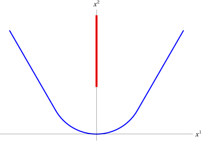
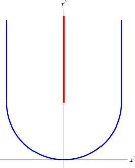
$\theta\in(0,\pi)$		$\theta=\pi$

Figure 1: The piecewise smooth curve (5) (symmetrically extended to $s\in\mathbb{R}$) and its cut-locus (red).

The surface $\Sigma_{\theta}$ can be regarded as a regularised version of the conical geometry considered in [19, 9, 35, 11]. Indeed, Theorem 1 applies to $\Sigma_{\theta}$ with $\theta\in(0,\pi)$, confirming in this way the results of the precedent works. In fact, not necessarily rotationally symmetric cones are considered in [35, 11], and moreover the accumulation rate of the eigenvalues is derived there. On the other hand, the strength of the present work is that we go substantially beyond the conical geometries, so the present paper can be considered as a generalisation of [35, 11].

The present paper can be also considered as a generalisation of our precedent work [26] to three dimensions. Indeed, our modus operandi is again rooted in developing the method of parallel coordinates based on $\Sigma$ involving the cut-locus of $\Sigma$. Unfortunately, the common limitation of the method is that we can consider special surfaces only: those for which the cut-locus is known explicitly. However, the unprecedented novelty with respect to [26] is that an asymptotic knowledge of the cut-locus is enough in the present work. This enables us to cover more general geometries. What is more, the present proof of the existence of discrete spectrum exhibits another important novelty with respect to the previous work: The argument requires a careful choice of the trial function localised at infinity. This is indeed a huge difference with respect to [26], where the trial function was the standard one, i.e. essentially a constant localised everywhere. This phenomenon is closely related to the existence of the intrinsic Gauss curvature $K$ for surfaces, while there are just extrinsic curvatures for curves. It has been noticed already in [10] that a more refined choice of trial functions is necessary for layers over surfaces with positive total Gauss curvature. Furthermore, the unconventional choice of the trial function enables one to conclude that there is actually an infinite number of discrete eigenvalues.

The paper is organised as follows. In Section 2 we develop a general approach to soft and leaky quantum layers, in particular we introduce a useful parameterisation of $\mathbb{R}^{3}$ involving the cut-locus of $\Sigma$. In Section 3 we consider the special situation of cylindrically symmetric layers. Theorem 1 is proved in Section 4.

2 Parallel coordinates

Let us first develop a general approach to study soft quantum layers. The first part of our approach (before speaking about the cut-locus) is rather standard and we refer to [6, 29] for similar geometric preliminaries.

Let $\Sigma$ be a connected orientable smooth surface in $\mathbb{R}^{3}$. We are particularly interested in non-compact complete surfaces, but $\Sigma$ can be alternatively compact in these geometric preliminaries. The induced metric of $\Sigma$ will be denoted by $g$. Introducing the standard notation $|g|:=\det(g)$, the surface element of $\Sigma$ reads $\mathrm{d}\Sigma=|g|^{1/2}\,\mathrm{d}s^{1}\wedge\mathrm{d}s^{2}$, where $(s^{1},s^{2})$ is a local coordinate system of $\Sigma$. The orientation of $\Sigma$ is specified by a globally defined unit normal vector field $n\in\Sigma\to\mathbb{S}^{2}$. For any $p\in\Sigma$, we introduce the Weingarten map

$$L:T_{p}\Sigma\to T_{p}\Sigma:\{\xi\mapsto-\mathrm{d}n(\xi)\}\,.$$

The eigenvalues $k_{1},k_{2}$ of $L$ are called the principal curvatures of $\Sigma$. They are defined only locally on $\Sigma$, but the Gauss curvature $K:=\det(L)=k_{1}k_{2}$ and the mean curvature $M:=\frac{1}{2}\mathop{\mathrm{tr}}\nolimits(L)=\frac{1}{2}(k_{1}+k_{2})$ are globally defined smooth functions on $\Sigma$. The relationship of $L$ with the second fundamental form $h$ of $\Sigma$ is through the formula $L^{\mu}_{\ \nu}=g^{\mu\rho}h_{\rho\nu}$ where $h=h_{\mu\nu}\mathrm{d}s^{\mu}\mathrm{d}s^{\nu}$, $g=g_{\mu\nu}\mathrm{d}s^{\mu}\mathrm{d}s^{\nu}$ and, as usual, $g^{\mu\nu}$ denote the entries of the inverse matrix $(g_{\mu\nu})^{-1}$. Here we adopt the Einstein summation convention, the range of Greek and Latin indices being $1,2$ and $1,2,3$, respectively.

The characteristic hypothesis of this work is that the Gauss curvature is integrable:

$$K\in L^{1}(\Sigma)$$. (6)

Then the total Gauss curvature $\mathcal{K}:=\int_{\Sigma}K\,\mathrm{d}\Sigma$ is well defined. The quantity $\mathcal{K}$ plays an important role in the global geometry of $\Sigma$. In fact, by the celebrated Gauss–Bonnet theorem (see, e.g., [25, Sec. 6.3]), $\mathcal{K}$ is a topological invariant for closed surfaces. By [23], the hypothesis (6) implies that $\Sigma$ is conformally equivalent to a closed surface from which a finite number of points have been removed.

Let us consider the normal exponential map

$$\Phi:\Sigma\times\mathbb{R}\to\mathbb{R}^{3}:\left\{(p,t)\mapsto p+n(p)\,t\right\}.$$ (7)

It gives rise to parallel (or Fermi) “coordinates” $(p,t)$ based on $\Sigma$. The metric $G$ induced by (7) has a block form

$$G=g\circ(I-tL)^{2}+\mathrm{d}t^{2}\,,$$ (8)

where $I$ denotes the identity map on $T_{p}\Sigma$. Consequently,

$$|G|:=\det(G)=|g|\,[\det(I-tL)]^{2}=|g|\,[(1-tk_{1})(1-tk_{2})]^{2}=|g|\,(1-2Mt+Kt^{2})^{2}\,.$$

The map $\Phi$ is standardly used in the theory of quantum layers as a convenient parametrisation of the tubular neighbourhood $\Omega_{a}$ introduced in (1). It follows by the inverse function theorem that the restricted map $\Phi:\Sigma\times(-a,a)\to\Omega_{a}$ is a local diffeomorphism provided that

$$\framebox{$0<a<\big{(}\max\left\{\|k_{1}\|_{\infty},\|k_{2}\|_{\infty}\right\}\big{)}^{-1}$}$$ (9)

(with the convention that the right hand side equals $\infty$ if the principal curvatures are identically equal to zero). Of course, to be able to satisfy this inequality with a positive $a$, it is necessary to assume that the Gauss and mean curvatures are globally bounded functions (this is automatically satisfied for compact $\Sigma$). The crucial requirement that the tubular neighbourhood (1) “does not overlap itself” precisely means that $\Phi:\Sigma\times(-a,a)\to\Omega_{a}$ is a (global) diffeomorphism, which is ensured by assuming in addition to (9) the ad hoc requirement that

$$\Phi\upharpoonright\Sigma\times(-a,a)$$  is injective. (10)

Then $\big{(}\Sigma\times(-a,a),G\big{)}$ is an embedded submanifold of $\mathbb{R}^{3}$ and $\Omega_{a}=\Phi\big{(}\Sigma\times(-a,a)\big{)}$ has indeed the geometrical meaning of the set of points in $\mathbb{R}^{3}$ squeezed between two parallel hypersurfaces at the distance $a$ from $\Sigma$. Indeed, within $\Omega_{a}$, one observes that $p\mapsto\Phi(p,t)$ is an embedded surface parallel to $\Sigma$ at the distance $|t|$ for any fixed $t\in(-a,a)$, while $t\mapsto\Phi(p,t)$ is a straight line (i.e. a geodesic in $\mathbb{R}^{3}$) orthogonal to $\Sigma$ at any fixed point $p\in\Sigma$.

Now we go beyond the standard approach to quantum layers by extending the parallel coordinates $\Phi$ from $\Omega_{a}$ to the whole space $\mathbb{R}^{3}$. We are inspired by [36, App. 1]. Define the cut-radius maps $c_{\pm}:\Sigma\to(0,\infty]$ by the property that the segment $t\mapsto\Phi(p,t)$ for positive (respectively, negative) $t$ minimises the distance from $\Sigma$ if, and only if, $t\in[0,c_{+}(p))$ (respectively, $t\in(-c_{-}(p),0]$). The cut-radius maps are known to be continuous. The cut-locus

$$\mathrm{Cut}(\Sigma):=\{\Phi(p,c_{+}(p)):p\in\Sigma\}\cup\{\Phi(p,-c_{-}(p)):p\in\Sigma\}$$ (11)

is a closed subset of $\mathbb{R}^{3}$ of measure zero (see, e.g., [7, Chap. III]). The map $\Phi$, when restricted to the set

$$U:=\{(p,t)\in\Sigma\times\mathbb{R}:\ -c_{-}(p)<t<c_{+}(p)\}$$ (12)

is a diffeomorphism onto $\Phi(U)=\mathbb{R}^{3}\setminus\mathrm{Cut}(\Gamma)$. Obviously, one has the inclusion

$$\mathrm{Cut}(\Sigma)\supset\mathrm{Cut}_{0}(\Sigma):=\big{\{}\Phi(p,t):\ 1-2M(p)\,t+K(p)\,t^{2}=0\big{\}}\,,$$ (13)

where $\mathrm{Cut}_{0}(\Sigma)$ is called the conjugate locus of $\Sigma$ (points where the Jacobian of $\Phi$ vanishes).

Outside the cut-locus, we have the usual coordinates of quantum layers. If $(s^{1},s^{2})$ is a local coordinate system of $\Sigma$, then $(s^{1},s^{2},t)$ is a natural local coordinate system of $\Phi(U)$. With respect to the corresponding coordinate frame, the metric $G$ admits the matrix representation

$$\big{(}G_{ij}\big{)}=\begin{pmatrix}\big{(}G_{\mu\nu}\big{)}&0\\ 0&1\end{pmatrix}\qquad\mbox{with}\qquad G_{\mu\nu}=g_{\mu\rho}(\delta^{\rho}_{\sigma}-tL^{\rho}_{\ \sigma})(\delta^{\sigma}_{\nu}-tL^{\sigma}_{\ \nu})\,.$$ (14)

In particular, the volume element of $\Phi(U)$ is given by

$$\mathrm{d}v:=(1-2Mt+Kt^{2})\,\mathrm{d}\Sigma\wedge\mathrm{d}t\,.$$

In agreement with [10], we say that a non-compact surface $\Sigma$ is asymptotically planar if the Gauss and mean curvatures vanish at infinity, which we schematically write as

$$K,M\xrightarrow[]{\ \infty\ }$$ 0. (15)

Recall that a function $f$, defined on a non-compact manifold $\Sigma$, is said to vanish at infinity if, given any positive number $\varepsilon$, there exists a compact subset $K\subset\Sigma$ such that $|f|<\varepsilon$ on $\Sigma\setminus K$. Similarly, we say that $f$ diverges at infinity and write $f\xrightarrow[]{\ \infty\ }\infty$ if, given any positive number $\varepsilon$, there exists a compact subset $K\subset\Sigma$ such that $|f|>\varepsilon^{-1}$ on $\Sigma\setminus K$. In parallel (15), we say that $\Sigma$ is asymptotically cut-locus planar if

$$c_{\pm}\xrightarrow[]{\ \infty\ }\infty$$. (16)

Note that (16) implies (15) due to the inclusion (13). On the other hand, we expect that the reverse implication does not hold in general.

Conjecture 1.

There exists a connected surface such that (15) holds but (16) is violated.

For possibly disconnected surfaces this is obvious (think about two parallel planes), but constructing an explicit connected example seems difficult (see Figure 2 for a partial attempt). A sufficient condition to ensure hypothesis (16) as a consequence of (15) is given by surfaces of revolutions (cf. Lemma 4 below).

Now we turn from geometric to analytic preliminaries. Recall our Hamiltonian $H$ given in (2). If $V:\mathbb{R}^{3}\to\mathbb{R}$ is an essentially bounded function (as is indeed the case of the soft realisation of the confinement), then $H$ can be introduced as an ordinary operator sum of the self-adjoint Laplacian with domain $H^{2}(\mathbb{R}^{3})$ and the maximal operator of multiplication generated by $V$. The associated closed form reads

$$h[u]:=\int_{\mathbb{R}^{3}}|\nabla u|^{2}+\int_{\mathbb{R}^{3}}V|u|^{2}\,,\qquad\mathop{\mathrm{dom}}\nolimits h:=H^{1}(\mathbb{R}^{3})\,.$$ (17)

If $V$ is the distribution of the leaky type $V_{\mathrm{leaky}}:=\alpha\delta_{\Sigma}$, the simplest is to start with the form (17), where the second term should be interpreted as $\alpha\int_{\Sigma}|u|^{2}$. Again, it is a well-defined and closed form under our standing hypothesis (9) and (10). In either case, $H$ can be defined as the self-adjoint operator associated with $h$ (with the properly interpreted second integral) via the representation theorem [24, Thm. VI.2.1].

Finally, we express $H$ in the parallel coordinates. This is achieved by means of the unitary map $\mathcal{U}:L^{2}(\mathbb{R}^{3})\to L^{2}(U,\mathrm{d}v)$ defined by $\mathcal{U}u:=u\circ\Phi$. Then $\hat{H}:=\mathcal{U}H\mathcal{U}^{-1}$ is the operator associated with the quadratic form $\hat{h}[\psi]:=h[\mathcal{U}^{-1}\psi]$ with $\mathop{\mathrm{dom}}\nolimits\hat{h}:=\mathcal{U}\mathop{\mathrm{dom}}\nolimits h$. Explicitly, using the block-diagonal form of the metric (8), one has

$$\hat{h}[\psi]=\int_{U}\overline{\partial_{\mu}\psi}\,G^{\mu\nu}\,\partial_{\nu}\psi\,\mathrm{d}v+\int_{U}|\partial_{t}\psi|^{2}\,\mathrm{d}v+\int_{U}W(t)\,|\psi|^{2}\,\mathrm{d}v\,,$$ (18)

where $(G^{\mu\nu}):=(G_{\mu\nu})^{-1}$. Hereafter the last integral should be interpreted as $\alpha\int_{\Sigma}|\psi(\cdot,0)|^{2}\,\mathrm{d}\Sigma$ in the case of leaky layers. In the sense of distributions, the operator $\hat{H}$ associated with $\hat{h}$ acts as

$$\hat{H}=-|G|^{-1/2}\partial_{\mu}|G|^{1/2}G^{\mu\nu}\partial_{\nu}-|G|^{-1/2}\partial_{t}|G|^{1/2}\partial_{t}+W\,.$$

Here $W$ is absent in the case of leaky layers, the influence of the Dirac interaction being realised by appropriate transmission conditions imposed on $\Sigma$ in the operator domain. We shall not need to specify this condition, for it is enough to work on the level of forms for our purposes.

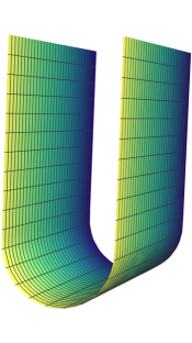
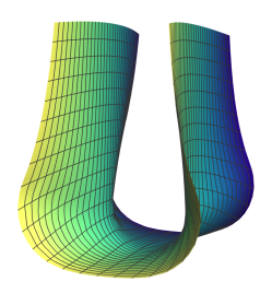
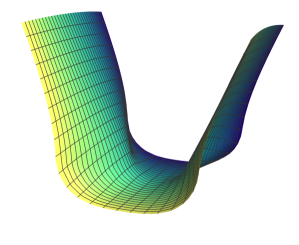
(a) asymptotically neither cut-locus planar nor planar	(b) asymptotically planar (along $x^{2}$) but not cut-locus planar	(c) asymptotically cut-locus planar (along $x^{2}$)

Figure 2: Towards the proof of Conjecture 1. Surface (a) is the curve of Figure 1 with $\theta=\pi$ and $R=1$ translated along axis $x^{3}$. Then it is not asymptotically cut-locus planar because the distance between the flat parts equals the constant $2$ as $x^{2}\to\infty$. Surface (b) is obtained from (a) by taking the radius $R$ in (5) dependent both on $s$ and $x^{3}$, namely $R(s,x^{3}):=1+(x^{3})^{2}/(1+s^{2})$. Then (b) is not asymptotically cut-locus planar either (the distance between the modified flat parts remains $2$ as $x^{2}\to\infty$ and $x^{3}=0$), while $K,M\to 0$ as $x^{2}\to\infty$ and $x^{3}$ is fixed (the challenge is to have (15) globally). Surface (c) is the curve of Figure 1 with $\theta=\frac{5}{7}\pi$ and $R$ as for (b); then $c_{\pm}\to\infty$ as $x^{2}\to\infty$ and $x^{3}$ is fixed.

3 Rotationally symmetric layers

The parallel coordinates of the previous section enables one to transfer the geometrically complicated action of the operator $H$ into the coefficients of the transformed operator $\hat{H}$. The problem is that even the form domain $\mathop{\mathrm{dom}}\nolimits\hat{h}$ is not easy to identify because of the boundary conditions on $\partial U$. An objective of this paper is to point out that there exists a special class of surfaces for which this is feasible because of a more precise information about the cut-locus. These are surfaces of revolution, so here we consider layers which are invariant with respect to rotations around a fixed axis in $\mathbb{R}^{3}$.

Let $r,z:[0,\infty)\to\mathbb{R}$ be smooth functions such that $r(s)>0$ for all $s>0$, $r(0)=0=z(0)$, $r^{\prime}(0)=1$ and

$$r^{\prime}(s)^{2}+z^{\prime}(s)^{2}=1$$ (19)

for all $s\geq 0$. The last identity implies that the planar curve $\Gamma(s):=(r(s),z(s))$ is unit-speed (see Figure 3). We consider the smooth surface of revolution $\Sigma$ obtained be revolving $\Gamma$ along the second axis:

$$\Sigma:=\left\{\left(r(s)\cos\vartheta,r(s)\sin\vartheta,z(s)\right):\ (s,\vartheta)\in[0,\infty)\times[0,2\pi)\right\}.$$ (20)

We use the following natural parametrisation of $\Sigma$:

$$p:(0,\infty)\times(0,2\pi)\to\mathbb{R}^{3}:\left\{(s,\vartheta)\mapsto\left(r(s)\cos\vartheta,r(s)\sin\vartheta,z(s)\right)\right\},$$ (21)

which gives rise to geodesic polar “coordinates” $(s,\vartheta)$ on $\Sigma$. With respect to these coordinates, the induced metric $g_{\mu\nu}:=\partial_{\mu}p\cdot\partial_{\nu}p$, where the dot denotes the scalar product in $\mathbb{R}^{3}$, reads

$$(g_{\mu\nu})=\begin{pmatrix}1&0\\ 0&r^{2}\end{pmatrix}.$$ (22)

In particular, the surface element of $\Sigma$ reads $\mathrm{d}\Sigma:=r(s)\,\mathrm{d}s\wedge\mathrm{d}\vartheta$. Because of the availability of a unique chart $p^{-1}$ (which covers the whole $\Sigma$ except for the curve $\Gamma$, which is a set of measure zero relative to $\Sigma$), we shall consider the geometric objects of $\Sigma$ as functions of $(s,\vartheta)$ rather than points of $\Sigma$.

With respect to the surface normal

$$n(s,\vartheta):=\left(-z^{\prime}(s)\cos\vartheta,-z^{\prime}(s)\sin\vartheta,r^{\prime}(s)\right),$$ (23)

we have the following formulae for the second fundamental form $h_{\mu\nu}:=-\partial_{\mu}n\cdot\partial_{\nu}p$ and the Weingarten tensor $L^{\mu}_{\ \nu}=g^{\mu\rho}h_{\rho\nu}$:

$$(h_{\mu\nu}) =\begin{pmatrix}r^{\prime}z^{\prime\prime}-r^{\prime\prime}z^{\prime}&0\\ 0&rz^{\prime}\end{pmatrix},$$ (24)

$$(L^{\mu}_{\ \nu}) =\begin{pmatrix}k_{1}&0\\ 0&k_{2}\end{pmatrix},\qquad\begin{aligned} k_{1}&:=r^{\prime}z^{\prime\prime}-r^{\prime\prime}z^{\prime}\,,\quad k_{2}:=\frac{z^{\prime}}{r}\,.\end{aligned}$$

Consequently, the layer metric (14) is actually diagonal. The principal curvatures $k_{1}$ and $k_{2}$ will be called the meridian and parallel curvatures, respectively. Because of the rotational symmetry, the curvatures are independent of $\vartheta$, so we suppress this variable from the arguments to simplify the notation.

Differentiating (19), we obtain the identity $r^{\prime}r^{\prime\prime}+z^{\prime}z^{\prime\prime}=0$. Using it in the definition of $K=k_{1}k_{2}$ with help of the formulae (24) for the principal curvatures, we arrive at the Jacobi equation

$$r^{\prime\prime}+Kr=0,$$ (25)

subject to initial conditions $r(0)=0$ and $r^{\prime}(0)=1$. The differential equation (25) has important consequences. First, we have the following upper bound on the Jacobian $r$.

Lemma 1.

Assume (6). Then there exists a positive constant $C_{\Sigma}$ such that

$$\forall s\geq 0\,,\qquad r(s)\leq C_{\Sigma}\,s\,.$$

Proof.

Integrating (25), we obtain the uniform bound

$$r^{\prime}(s)=1-\int_{0}^{s}(Kr)(s)\,\mathrm{d}s\leq 1+\frac{\|K\|_{L^{1}(\Sigma)}}{2\pi}=:C_{\Sigma}$$

for all $s\geq 0$. Integrating this inequality, we obtain the desired claim. ∎

Second, (25) implies the Gauss–Bonnet theorem

$$\mathcal{K}=2\pi\,[1-r^{\prime}(\infty)]\,,\qquad\mbox{where}\qquad r^{\prime}(\infty):=\lim_{s\to\infty}r^{\prime}(s)\,.$$ (26)

Note that the limit is well defined as a consequence of this equality and hypothesis (6). Necessarily,

$$0\leq\mathcal{K}\leq 2\pi\,.$$ (27)

Here the non-negativity follows from (19), while the upper bound is valid due to the positivity of $r$. If the total Gauss curvature $\mathcal{K}$ is positive, we get an important information on the parallel curvature.

Lemma 2.

Assume (6) with $\mathcal{K}>0$. There exist positive numbers $\delta$ and $s_{0}$ such that

$$\forall s\geq s_{0}\,,\qquad\frac{\delta}{r(s)}\leq|k_{2}(s)|\leq\frac{1}{r(s)}\,.$$

Proof.

The lemma is due to [10, Lem. 6.1], we repeat the proof to make the presentation self-contained. By (27), (26) and the assumption $\mathcal{K}>0$, one has $0\leq r^{\prime}(\infty)<1$. It follows that there exist $\delta^{\prime}\in(0,\frac{1}{2})$ and $s_{0}>0$ such that $-\delta^{\prime}\leq r^{\prime}(s)\leq 1-\delta^{\prime}$ for all $s\geq s_{0}$. Then the desired claim follows from the definition of $k_{2}$. ∎

It follows from Lemmata 1 and 2 that $k_{2}$ is not integrable, i.e., $k_{2}\not\in L^{1}((0,\infty))$. On the other hand, the meridian curvature $k_{1}$ is integrable, which follows from the smoothness of $r,z$ and the following estimates:

$$\infty>\frac{\|K\|_{L^{1}(\Sigma)}}{2\pi}\geq\int_{s_{0}}^{\infty}|k_{1}(s)k_{2}(s)|\,r(s)\,\mathrm{d}s\geq\delta\int_{s_{0}}^{\infty}|k_{1}(s)|\,\mathrm{d}s\,.$$ (28)

Consequently, $M\not\in L^{1}((0,\infty))$. This is the essence of our subsequent analysis: Even if $M$ may decay at infinity, it is not negligible in the integral sense there.

Since $\Sigma$ is rotationally symmetric, the cut-radius maps $c_{\pm}$ do not depend on the angular variable, so we may suppress it from the argument. The map $\Phi$ defined in (7), when restricted to the open set

$$U:=\{(s,\vartheta,t)\in(0,\infty)\times(0,2\pi)\times\mathbb{R}:-c_{-}(s)<t<c_{+}(s)\}$$ (29)

is a diffeomorphism onto $\Phi(U)=\mathbb{R}^{3}\setminus\{(x^{1},0,x^{3}):x^{1}\geq 0,x^{3}\in\mathbb{R}\}$. Since the latter coincides with $\mathbb{R}^{3}$ up to a set of measure zero, the map $\Phi$ can be used as a parametrisation of $\mathbb{R}^{3}$.

The basic hypothesis (9) is obviously satisfied (with a positive $a$) due to (15) and smoothness of $\Sigma$. The global requirement (10) must still be satisfied ad hoc due to possible self-crossings of $\Gamma$. The following observation shows, however, that it is actually enough to exclude the self-crossings only locally.

Lemma 3.

Assume (6) and (15). Then $r(s)\to\infty$ as $s\to\infty$.

Proof.

If (6) holds with $\mathcal{K}>0$, then the result follows from Lemma 2 (note that $K,M$ vanish at infinity if, and only if, $k_{1},k_{2}$ vanish at infinity). If $\mathcal{K}=0$, then $r^{\prime}(\infty)=1$. But then $r(s)=r(s_{0})+\int_{s_{0}}^{s}r^{\prime}\geq\frac{1}{2}(s-s_{0})$ for all sufficiently large $s_{0}<s$. Fixing $s_{0}$ and sending $s$ to $\infty$, we get the desired claim. ∎

Our main hypothesis for rotationally symmetric layers is that the cut-locus of $\Sigma$ asymptotically coincides with the upper part of the axis of symmetry:

$$\exists R_{0}>0\,,\qquad\mathrm{Cut}(\Sigma)\setminus B_{R_{0}}(0)=\big{\{}(0,0,x^{3}):x^{3}\geq R_{0}\big{\}}$$. (30)

Lemma 4.

Assume (6) with $\mathcal{K}>0$, (15) and (30). Then there exists $s_{0}>0$ such that, for all $s\geq s_{0}$, $k_{1}(s)\geq 0$, $k_{2}(s)>0$, $c_{-}(s)=\infty$, $c_{+}(s)=1/k_{2}(s)$ and $k_{1}(s)\leq k_{2}(s)$.

Proof.

The crucial observation is that $r(s)\to\infty$ as $s\to\infty$ as a consequence of Lemma 2 and (15) (or see directly Lemma 3). At the same time, $z(s)\to\pm\infty$ as $s\to\infty$ because $z^{\prime}(\infty)^{2}=1-r^{\prime}(\infty)^{2}>0$, where the inequality is implied by $\mathcal{K}>0$ and (26). Then $c_{-}(s)=\infty$ and $c_{+}(s)=1/k_{2}(s)$ for all sufficiently large $s$. Indeed, by (30) and the symmetry, for all sufficiently large $s$ and any $\vartheta\in[0,2\pi)$, the curve $\gamma(t):=p(s,\vartheta)+n(s,\vartheta)t$ does not intersect the ball $B_{R_{0}}(0)$, so the only intersection must be with the semi-axis $\big{\{}(0,0,x^{3}):x^{3}\geq R_{0}\big{\}}$. Moreover, $\gamma^{1}(t)=0$ implies $t=r/z^{\prime}=1/k_{2}$. This argument also excludes the possibility $z(s)\to-\infty$ as $s\to\infty$, because otherwise the curve $\gamma$ would intersect the negative semi-axis $\{(0,0,x^{3}):x^{3}\leq-R_{0}\}$ for all sufficiently large $s$. Consequently, $z^{\prime}(\infty)>0$, so the parallel curvature $k_{2}(s)$ is positive for all sufficiently large $s$. We claim that the meridian curvature $k_{1}(s)$ is non-negative for all sufficiently large $s$ (see Figure 3). Indeed, if it is not the case, then there exist large positive numbers $s_{1}<s_{2}$ such that the graph of the curve $\Gamma$ is strictly concave on $(s_{1},s_{2})$, implying the existence of a cut-locus of $\Gamma$ to the right of the curve (when traced according to the arc-length parameter), therefore violating (30). Finally, if $k_{1}(s)>k_{2}(s)$, then $1/k_{1}(s)<1/k_{2}(s)=c_{+}(s)$, implying a contradiction that there exists a conjugate point outside the cut-locus. ∎

There are many surfaces of revolution satisfying (30). For instance, if $s\mapsto\Gamma(s)$ is a convex graph, then $c_{-}(s)=\infty$ for all $s\geq 0$, so there is no cut-locus “outside” of $\Sigma$ (i.e. for negative $t$). To show that the cut-locus satisfies (30) “inside” of $\Sigma$ (i.e. for positive $t$), one can employ the geometric interpretation of the principal curvatures (minimal and maximal values of the normal curvatures of all the curves passing through a given point). Then it is easy to verify that (30) can be achieved as a consequence (15) (still assuming (6) with $\mathcal{K}>0$). In particular, the paraboloid of revolution satisfies (30) (as well as (6) with $\mathcal{K}=2\pi$ and (15)).

To be even more explicit, let us consider the family of surfaces $\Sigma_{\theta}$ obtained be revolving the planar curve (5). The cut-locus of $\Sigma_{\theta}$ is the semi-axis $\{(0,0,x^{3}):x^{3}\geq R\}$ if $\theta\in(0,\pi]$, while it is empty if $\theta=0$. Of course, $\Sigma_{\theta}$ is not smooth (unless $\theta=0$), but it is piecewise smooth (in fact, piecewise analytic). The total Gauss curvature of $\Sigma_{\theta}$ reads

$$\mathcal{K}_{\theta}=2\pi(1-\cos\mbox{$\frac{\theta}{2}$})\,,$$ (31)

so the hypotheses of Lemma 2 are met whenever $\theta\in(0,\pi)$.

Finally, we make a hypothesis about a sufficient decay of the parallel curvature at infinity:

$$\exists\epsilon>0\,,\qquad k_{2}(s)=O(s^{-\epsilon})\qquad\mbox{as}\qquad s\to\infty$$. (32)

This condition (with $\epsilon=1$) is easily verified for $\Sigma_{\theta}$ whenever $\theta\in[0,\pi)$. It also holds for the paraboloid of revolution (with $\epsilon=1/2$) and other surfaces obtained by revolving polynomially growing curves.

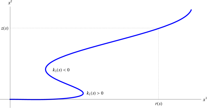
Figure 3: The geometry of the generating curve $\Gamma$.

4 The proofs

We assume that the potential $V$ is either the distribution $V_{\mathrm{leaky}}:=\alpha\delta_{\Sigma}$ with $\alpha<0$ or it is an essentially bounded function satisfying (3) and (4). Let $E_{1}<0$ denote the lowest discrete eigenvalue of $T$. The variational characterisation yields

$$E_{1}=\inf_{\stackrel{{\scriptstyle[}}{{\xi}}\not=0]{}{\xi\in H^{1}(\mathbb{R})}}\frac{\displaystyle\int_{\mathbb{R}}|\xi^{\prime}(t)|^{2}\,\mathrm{d}t+\int_{\mathbb{R}}W(t)\,|\xi(t)|^{2}\,\mathrm{d}t}{\displaystyle\int_{\mathbb{R}}|\xi(t)|^{2}\,\mathrm{d}t}\,.$$ (33)

In the leaky case, the integral $\int_{\mathbb{R}}W(t)\,|\xi(t)|^{2}\,\mathrm{d}t$ should be interpreted as $\alpha\,|\xi(0)|^{2}$, in which case, explicitly, $E_{1}=-\frac{\alpha^{2}}{4}$. It is well known that $E_{1}$ is simple and that the corresponding eigenfunction $\xi_{1}$ can be chosen to be positive. We additionally choose the eigenfunction to be normalised to $1$ in $L^{2}(\mathbb{R})$, i.e., $\|\xi_{1}\|_{L^{2}(\mathbb{R})}=1$. Explicitly, $\xi_{1}(t)=\sqrt{\frac{|\alpha|}{4}}e^{\frac{\alpha}{2}|t|}$ in the leaky case. In any case, one knows that $\xi_{1}\in H^{1}(\mathbb{R})\cap L^{\infty}(\mathbb{R})$ and that the following identities hold true:

$$\xi_{1}(t)=N_{\pm}e^{\mp\sqrt{-E_{1}}t}\qquad\mbox{for every}\qquad\pm t>a\,,$$ (34)

where $N_{\pm}$ are positive constants.

Remark 1.

In principle, the assumption $\mathop{\mathrm{supp}}\nolimits W\subset[-a,a]$ of (3) could be relaxed to a decay of $W$ at infinity. Then the asymptotics (34) could be replaced by Agmon-type estimates.

First of all, we locate the essential spectrum of $H$ (assuming $\mathop{\mathrm{supp}}\nolimits W\subset[-a,a]$ or the leaky setting). As an auxiliary quantity, in parallel with (33), we consider

$$E_{1}^{b}:=\inf_{\stackrel{{\scriptstyle[}}{{\xi}}\not=0]{}{\xi\in H^{1}((-b,b))}}\frac{\displaystyle\int_{-b}^{b}|\xi^{\prime}(t)|^{2}\,\mathrm{d}t+\int_{-b}^{b}W(t)\,|\xi(t)|^{2}\,\mathrm{d}t}{\displaystyle\int_{-b}^{b}|\xi(t)|^{2}\,\mathrm{d}t}\,,$$ (35)

where $b>a$. Of course, $E_{1}^{b}$ is the lowest eigenvalue of the operator $T$ restricted to $(-b,b)$, subject to Neumann boundary conditions.

Lemma 5.

One has

$$\lim_{b\to\infty}E_{1}^{b}=E_{1}\,.$$

Proof.

In the leaky case, $E_{1}^{b}$ solves the implicit equation $2\sqrt{-E}=-\alpha\coth(\sqrt{-E}b)$, from which the convergence can be easily deduced. In the regular case, let us assume $b>a$. By using $\xi_{1}$ (or, more precisely, its restriction to $(-b,b)$) as a trial function in (35), it is easy to see that

$$E_{1}^{b}\leq E_{1}\,.$$ (36)

To get an opposite estimate, let $\xi_{1}^{b}$ be the positive minimiser of (35) normalised to $1$ in $L^{2}((-b,b))$. We extend it to the whole line by setting

$$\tilde{\xi}_{1}^{b}(t):=\begin{cases}\xi_{1}^{b}(t)&\mbox{if}\quad|t|<b\,,\\ \xi_{1}^{b}(\pm b)\,\exp\big{(}{\mp\sqrt{-E_{1}}(t\mp b)}\big{)}&\mbox{if}\quad\pm t\geq b\,.\end{cases}$$

Since $\tilde{\xi}_{1}^{b}\in H^{1}(\mathbb{R})$, we use it as a trial function in (33) and obtain

$$E_{1}\leq\frac{E_{1}^{b}+\frac{1}{2}\sqrt{-E_{1}}\,[\xi_{1}^{b}(-b)^{2}+\xi_{1}^{b}(b)^{2}]}{1+\frac{1}{2}\frac{1}{\sqrt{-E_{1}}}\,[\xi_{1}^{b}(-b)^{2}+\xi_{1}^{b}(b)^{2}]}\,.$$

It remains to notice that $\xi_{1}^{b}(\pm b)\to 0$ as $b\to\infty$. To see it, we employ the explicit solution

$$\xi_{1}^{b}(t)=\xi_{1}^{b}(\pm b)\,\cosh\big{(}\mbox{$\sqrt{-E_{1}^{b}}$}\,(t\mp b)\big{)}\qquad\mbox{for}\qquad a\leq\pm t\leq b\,.$$

Take $t=\pm a$ and use that the value $\xi_{1}^{b}(\pm a)$ can be estimated by the $H^{1}((-a,a))$ norm of $\xi_{1}^{b}$ as follows:

$$\xi_{1}^{b}(\pm a)^{2}\leq\int_{-a}^{a}|{\xi_{1}^{b}}^{\prime}(t)|^{2}\,\mathrm{d}t+C_{a}\int_{-a}^{a}|{\xi_{1}^{b}}(t)|^{2}\,\mathrm{d}t\,,$$

where explicitly $C_{a}:=1+(2a)^{-1}$. In turn, the right-hand side can be estimated by using the identity

$$\int_{-b}^{b}|{\xi_{1}^{b}}^{\prime}(t)|^{2}\,\mathrm{d}t+\int_{-b}^{b}W(t)\,|\xi_{1}^{b}(t)|^{2}\,\mathrm{d}t=E_{1}^{b}\int_{-b}^{b}|\xi_{1}^{b}(t)|^{2}\,\mathrm{d}t\,.$$

Consequently, $\xi_{1}^{b}(\pm a)^{2}\leq\|W\|_{\infty}+C_{a}$. Finally, we obtain the exponential decay

$$\xi_{1}^{b}(\pm b)\leq\frac{\sqrt{\|W\|_{\infty}+C_{a}}}{\cosh\big{(}\mbox{$\sqrt{-E_{1}^{b}}$}\,(a\mp b)\big{)}}\xrightarrow[b\to\infty]{}0\,.$$

This concludes the proof of the lemma. ∎

The following theorem does not require that $\Sigma$ is a surface of revolution.

Theorem 2.

Let $\Sigma$ be an orientable smooth surface which is asymptotically cut-locus planar (16). Let the tubular neighbourhood (1) does not overlap itself with some positive $a$, i.e. (9) and (10) hold. Let $V$ satisfy (3) and (4). Then

$$\inf\sigma_{\mathrm{ess}}(H)\geq E_{1}\,.$$

Proof.

Fixing a point $p_{0}\in\Sigma$ and giving any positive number $R$, we divide the surface $\Sigma$ into two parts $\Sigma_{\mathrm{int}}:=\Sigma\cap B_{R}(p_{0})$ and $\Sigma_{\mathrm{ext}}:=\Sigma\setminus\overline{B_{R}(p_{0})}$, where $B_{R}(p_{0})$ is the geodesic ball of radius $R$ centred at $p_{0}$. Correspondingly, we divide the set $U$ into two parts

$$U_{\mathrm{int}} :=\{(p,t)\in\Sigma_{\mathrm{int}}\times\mathbb{R}:\ -c_{-}(p)<t<c_{+}(p)\}\,,$$

$$U_{\mathrm{ext}} :=\{(p,t)\in\Sigma_{\mathrm{ext}}\times\mathbb{R}:\ -c_{-}(p)<t<c_{+}(p)\}\,.$$

The interior part is further subdivided into two subparts

$$U_{\mathrm{int,1}} :=\{(p,t)\in\Sigma_{\mathrm{int}}\times\mathbb{R}:\ -a<t<a\}\,,$$

$$U_{\mathrm{int,2}} :=\{(p,t)\in\Sigma_{\mathrm{int}}\times\mathbb{R}:\ -c_{-}(p)<t<-a\ \lor\ a<t<c_{+}(p)\}\,.$$

Analogously, we subdivide $U_{\mathrm{ext}}$ into two subparts

$$U_{\mathrm{ext,1}} :=\{(p,t)\in\Sigma_{\mathrm{ext}}\times\mathbb{R}:\ -b<t<b\}\,,$$

$$U_{\mathrm{ext,2}} :=\{(p,t)\in\Sigma_{\mathrm{ext}}\times\mathbb{R}:\ -c_{-}(p)<t<-b\ \lor\ b<t<c_{+}(p)\}\,,$$

where $b>0$. By (16), we can assume $b>a$ by choosing $R$ large enough. Define

$$c_{R}^{\pm}:=1\pm 2\,\|M\|_{R}\,b\pm\|K\|_{R}\,b^{2}\qquad\mbox{with}\qquad\|\cdot\|_{R}:=\|\cdot\|_{L^{\infty}(\Sigma_{\mathrm{ext}})}\,.$$

Since (16) implies (15), given any (large) $b>a$, there exists (large) $R$ such that $c_{R}^{-}$ is positive.

We consider the auxiliar operator $\hat{H}^{N}$ which is obtained from $\hat{H}$ by impossing an extra Neumann condition (i.e. no condition on the level of sesquilinear forms) on the boundaries of the subsets described above. More specifically, $\hat{H}^{N}=\hat{H}_{\mathrm{int,1}}^{N}\oplus\hat{H}_{\mathrm{int,2}}^{N}\oplus\hat{H}_{\mathrm{ext}}^{N}$, where $\hat{H}_{\mathrm{ext}}^{N}=\hat{H}_{\mathrm{ext,1}}^{N}\oplus\hat{H}_{\mathrm{ext,2}}^{N}$ is the self-adjoint operator associated with the form $\hat{h}_{\mathrm{ext}}^{N}$ in $L^{2}(U_{\mathrm{ext}},\mathrm{d}v)$ defined by

$$\hat{h}_{\mathrm{ext}}^{N}[\psi] :=\int_{U_{\mathrm{ext}}}\overline{\partial_{\mu}\psi}\,G^{\mu\nu}\,\partial_{\nu}\psi\,\mathrm{d}v+\int_{U_{\mathrm{ext}}}|\partial_{t}\psi|^{2}\,\mathrm{d}v+\int_{U_{\mathrm{ext}}}W(t)\,|\psi|^{2}\,\mathrm{d}v\,,$$

$$\mathop{\mathrm{dom}}\nolimits\hat{h}_{\mathrm{ext}}^{N}[\psi] :=\big{\{}\psi\upharpoonright\hat{h}_{\mathrm{ext}}:\ \psi\in\mathop{\mathrm{dom}}\nolimits\hat{h}\big{\}}\,,$$

and similarly for the other operators. Obviously, $\mathop{\mathrm{dom}}\nolimits\hat{h}^{N}\supset\mathop{\mathrm{dom}}\nolimits\hat{h}$, therefore $\hat{H}^{N}\leq\hat{H}$ in the sense of quadratic forms, so, by the minimax principle, it is enough to show that $\inf\sigma_{\mathrm{ess}}(\hat{H}^{N})\geq E_{1}$. Since $\mathop{\mathrm{supp}}\nolimits W\subset[-a,a]$ due to (3), the operator $\hat{H}_{\mathrm{int,2}}^{N}$ is non-negative, so the inequality $\inf\sigma_{\mathrm{ess}}(\hat{H}_{\mathrm{int,2}}^{N})\geq E_{1}$ is trivial. At the same time, $\hat{H}_{\mathrm{int,1}}^{N}$ is an operator with compact resolvent, so it does not contribute to the essential spectrum of $\hat{H}^{N}$ (one has $\inf\sigma_{\mathrm{ess}}(\hat{H}_{\mathrm{int,1}}^{N})=\infty$ by the minimax principle). It remains to estimate the essential spectrum of $\hat{H}_{\mathrm{ext}}^{N}$.

For every $\psi\in\mathop{\mathrm{dom}}\nolimits\hat{h}_{\mathrm{ext}}^{N}$,

$$\hat{h}_{\mathrm{ext}}^{N}[\psi] \geq\int_{U_{\mathrm{ext}}}|\partial_{t}\psi|^{2}\,\mathrm{d}v+\int_{U_{\mathrm{ext}}}W(t)\,|\psi|^{2}\,\mathrm{d}v$$

$$\geq\int_{U_{\mathrm{ext,1}}}|\partial_{t}\psi|^{2}\,\mathrm{d}v+\int_{U_{\mathrm{ext,1}}}W(t)\,|\psi|^{2}\,\mathrm{d}v$$

$$\geq c_{R}^{-}\int_{U_{\mathrm{ext,1}}}|\partial_{t}\psi|^{2}\,\mathrm{d}\Sigma\,\mathrm{d}t+\int_{U_{\mathrm{ext,1}}}W(t)\,|\psi|^{2}\,\mathrm{d}v$$

$$\geq c_{R}^{-}\,E_{1}^{b}\int_{U_{\mathrm{ext,1}}}|\psi|^{2}\,\mathrm{d}\Sigma\,\mathrm{d}t-c_{R}^{-}\int_{U_{\mathrm{ext,1}}}W(t)\,|\psi|^{2}\,\mathrm{d}\Sigma\,\mathrm{d}t+\int_{U_{\mathrm{ext,1}}}W(t)\,|\psi|^{2}\,\mathrm{d}v$$

$$\geq\frac{c_{R}^{-}}{c_{R}^{+}}\,E_{1}^{b}\,\|\psi\|_{L^{2}(U_{\mathrm{ext}},\mathrm{d}v)}^{2}-c_{R}^{-}\int_{U_{\mathrm{ext,1}}}W(t)\,|\psi|^{2}\,\mathrm{d}\Sigma\,\mathrm{d}t+\int_{U_{\mathrm{ext,1}}}W(t)\,|\psi|^{2}\,\mathrm{d}v$$

where the fourth inequality employs the variational definition of $E_{1}^{b}$ (cf. (35)) with help of Fubini’s theorem and the fact that $\mathop{\mathrm{supp}}\nolimits W\subset[-a,a]$. Since

$$\int_{U_{\mathrm{ext,1}}}W(t)\,|\psi|^{2}\,\mathrm{d}v\geq\int_{U_{\mathrm{ext,1}}}c_{R}(t)\,W(t)\,|\psi|^{2}\,\mathrm{d}\Sigma\,\mathrm{d}t\,,$$

where $c_{R}(t):=c_{R}^{-}$ if $W(t)\geq 0$ and $c_{R}(t):=c_{R}^{+}$ if $W(t)<0$, we get

$$\hat{h}_{\mathrm{ext}}^{N}[\psi] \geq\frac{c_{R}^{-}}{c_{R}^{+}}\,E_{1}^{b}\,\|\psi\|_{L^{2}(U_{\mathrm{ext}},\mathrm{d}v)}^{2}-(c_{R}^{+}-c_{R}^{-})\int_{U_{\mathrm{ext,1}}}\chi_{\{W(t)<0\}}(t)\,|W(t)|\,|\psi|^{2}\,\mathrm{d}\Sigma\,\mathrm{d}t$$

$$\geq\left(\frac{c_{R}^{-}}{c_{R}^{+}}\,E_{1}^{b}-\frac{c_{R}^{+}-c_{R}^{-}}{c_{R}^{-}}\,\|W\|_{\infty}\right)\|\psi\|_{L^{2}(U_{\mathrm{ext}},\mathrm{d}v)}^{2}\,.$$

In summary,

$$\inf\sigma_{\mathrm{ess}}(\hat{H})\geq\inf\sigma_{\mathrm{ess}}(\hat{H}_{\mathrm{ext}}^{N})\geq\inf\sigma(\hat{H}_{\mathrm{ext}}^{N})\geq\frac{c_{R}^{-}}{c_{R}^{+}}\,E_{1}^{b}-\frac{c_{R}^{+}-c_{R}^{-}}{c_{R}^{-}}\,\|W\|_{\infty}\,.$$

Since $c_{R}^{-}/c_{R}^{+}\to 1$ as $R\to\infty$ due to (15) (which is a consequence of (16)), we obtain $\inf\sigma_{\mathrm{ess}}(\hat{H})\geq E_{1}^{b}$. Finally, the arbitrariness of $b$ and Lemma 5 yield that $\inf\sigma_{\mathrm{ess}}(\hat{H})\geq E_{1}$. ∎

We leave as an open problem whether $\sigma_{\mathrm{ess}}(H)\supset[E_{1},\infty)$ under the hypotheses of Theorem 2.

Now we turn to the existence of bound states. We heavily rely on results in Section 3 for rotationally symmetric layers. In particular, recall that, under the hypotheses of the following theorem: the surface Jacobian $r(s)$ is bounded from above by a multiple of $s$ (Lemma 1) and diverges as $s\to\infty$ (Lemma 3); the parallel curvature $k_{2}$ behaves like $r^{-1}$ (Lemma 2); the cut-radius maps satisfy $c_{-}(s)=\infty$ and $c_{+}(s)=k_{2}(s)^{-1}$ for all sufficiently large $s$ (Lemma 4); and thus (16) follows as a consequence of (15).

Theorem 3.

Let $\Sigma$ be a surface of revolution given by (20) and satisfying (6) with $\mathcal{K}>0$ and (15). Let $V$ satisfy (3) with some positive $a$ and (4). Assume in addition (30) and (32). Then $H$ possesses an infinite number (counting multiplicities) of discrete eigenvalues below $E_{1}$.

Proof.

In view of Theorem 2, to establish the existence of a discrete eigenvalue of $H$, it is enough to show that $\inf\sigma(H)<E_{1}$. By the minimax principle, it is thus enough to find a trial function $\psi\in\mathop{\mathrm{dom}}\nolimits Q:=\mathop{\mathrm{dom}}\nolimits\hat{h}$ such that $Q[\psi]:=\hat{h}[\psi]-E_{1}\,\|\psi\|^{2}<0$, where $\|\cdot\|$ denotes the norm in $L^{2}(U,\mathrm{d}v)$. Recall that, in the rotationally symmetric case, we have

$$\hat{h}[\psi] =\int_{U}|\partial_{s}\psi(s,\vartheta,t)|^{2}\,\frac{1-k_{2}(s)t}{1-k_{1}(s)t}\,\mathrm{d}\Sigma\,\mathrm{d}t+\int_{U}\frac{|\partial_{\vartheta}\psi(s,\vartheta,t)|^{2}}{r(s)^{2}}\,\frac{1-k_{1}(s)t}{1-k_{2}(s)t}\,\mathrm{d}\Sigma\,\mathrm{d}t$$ (37)

$$\quad+\int_{U}|\partial_{t}\psi(s,\vartheta,t)|^{2}\,(1-k_{1}(s)t)(1-k_{2}(s)t)\,\mathrm{d}\Sigma\,\mathrm{d}t$$

$$\|\psi\|^{2} =\int_{U}|\psi(s,\vartheta,t)|^{2}\,(1-k_{1}(s)t)(1-k_{2}(s)t)\,\mathrm{d}\Sigma\,\mathrm{d}t\,,$$

where $\mathrm{d}\Sigma=r(s)\,\mathrm{d}s\wedge\mathrm{d}\vartheta$ and $U$ is given by (29).

For every real $\varepsilon$, we introduce a $\vartheta$-independent trial function

$$\psi_{n,\varepsilon}(s,\vartheta,t):=\varphi_{n}(s)\,\xi_{1}(t)+\varepsilon\,\phi_{n}(s)\,t\,\xi_{1}(t)\,,$$

where the sequence $\{\varphi_{n}\}_{n=2}^{\infty}$ is defined by

$$\varphi_{n}(s):=\begin{cases}0&\mbox{if}\quad s\in[0,n)\,,\\ \displaystyle\frac{\log(s/n)}{\log n}&\mbox{if}\quad s\in[n,n^{2})\,,\\ \displaystyle\frac{\log(n^{3}/s)}{\log n}&\mbox{if}\quad s\in[n^{2},n^{3})\,,\\ 0&\mbox{if}\quad s\in[n^{3},\infty)\,,\end{cases}\qquad\mbox{and}\qquad\phi_{n}(s):=\frac{\varphi_{n}(s)}{s}\,.$$

Note that the supports of $\varphi_{n}$ and $\phi_{n}$ tend to infinity as $n\to\infty$. We always assume that $n$ is so large that the asymptotic properties of Lemma 4 hold. Proceeding as in [26, Lem. 1] (see also below), one can verify that $\psi_{n,\varepsilon}\in\mathop{\mathrm{dom}}\nolimits Q$. Then

$$Q[\psi_{n,\varepsilon}]=Q[\varphi_{n}\xi_{1}]+2\varepsilon\,Q\big{(}\phi_{n}t\xi_{1},\varphi_{n}\xi_{1}\big{)}+\varepsilon^{2}\,Q[\phi_{n}t\xi_{1}]\,.$$ (38)

We make the decomposition $Q=Q_{1}+Q_{2}$, where $Q_{1}[\psi]:=\int_{U}\overline{\partial_{\mu}\psi}\,G^{\mu\nu}\,\partial_{\nu}\psi\,\mathrm{d}v$ is just the first line of (37).

$Q_{1}$ One has

$$Q_{1}[\varphi_{n}\xi_{1}]=\int_{U}\varphi_{n}^{\prime}(s)^{2}\,\xi_{1}(t)^{2}\,f(s,t)\,\mathrm{d}\Sigma\,\mathrm{d}t\qquad\mbox{with}\qquad f(s,t):=\frac{1-k_{2}(s)t}{1-k_{1}(s)t}\geq 0\,.$$

Since

$$\partial_{t}f(\cdot,t)=\frac{k_{1}-k_{2}}{(1-k_{1}t)^{2}}\leq 0\,,$$

where the inequality holds due to Lemma 4, one has $\|f\|_{\infty}=1$. Consequently,

$$Q_{1}[\varphi_{n}\xi_{1}] \leq\int_{U}\varphi_{n}^{\prime}(s)^{2}\,\xi_{1}(t)^{2}\,\mathrm{d}\Sigma\,\mathrm{d}t$$

$$\leq 2\pi C_{\Sigma}\int_{0}^{\infty}\varphi_{n}^{\prime}(s)^{2}\,s\,\mathrm{d}s$$

$$=\frac{4\pi C_{\Sigma}}{\log n}\,,$$

where the second inequality holds due to Lemma 1 and the normalisation of $\xi_{1}$. Similarly,

$$Q_{1}[\phi_{n}t\xi_{1}]\leq\frac{4\pi CC_{\Sigma}}{n^{2}\log n}\,,\qquad\mbox{where}\qquad C:=\int_{\mathbb{R}}\xi_{1}(t)^{2}\,t^{2}\,\mathrm{d}t\,,$$

where the extra decay $n^{-2}$ comes from the bound $s\geq n$ on the support of $\phi_{n}$. The mixed term $Q_{1}\big{(}\phi_{n}t\xi_{1},\varphi_{n}\xi_{1}\big{)}$ tend to zero as $n\to\infty$ by using these estimates and the Schwarz inequality. In summary,

$$\lim_{n\to\infty}Q_{1}[\psi_{n,\varepsilon}]=0\,.$$

$Q_{2}$, order $\varepsilon^{0}$ One has

$$Q_{2}[\varphi_{n}\xi_{1}] =\int_{U}\varphi_{n}(s)^{2}\,\xi_{1}^{\prime}(t)^{2}\,(1-2M(s)t+K(s)t^{2})\,\mathrm{d}\Sigma\,\mathrm{d}t$$ (39)

$$\quad+\int_{U}W(t)\,\varphi_{n}(s)^{2}\,\xi_{1}(t)^{2}\,(1-2M(s)t+K(s)t^{2})\,\mathrm{d}\Sigma\,\mathrm{d}t$$

$$\quad-E_{1}\int_{U}\varphi_{n}(s)^{2}\,\xi_{1}(t)^{2}\,(1-2M(s)t+K(s)t^{2})\,\mathrm{d}\Sigma\,\mathrm{d}t$$

$$=\int_{U}|\varphi_{n}(s)|^{2}\xi_{1}(t)\xi_{1}^{\prime}(t)\,(2M(s)-2K(s)t)\,\mathrm{d}\Sigma\,\mathrm{d}t$$

$$\quad+\int_{\Sigma}|\varphi_{n}(s)|^{2}\left[\xi_{1}(t)\xi^{\prime}_{1}(t)(1-2M(s)t+K(s)t^{2})\right]_{t=-c_{-}(s)}^{t=c_{+}(s)}\,\mathrm{d}\Sigma$$

$$=\int_{U}|\varphi_{n}(s)|^{2}\,|\xi_{1}(t)|^{2}\,K(s)\,\mathrm{d}\Sigma\,\mathrm{d}t$$

$$\quad+\int_{\Sigma}|\varphi_{n}(s)|^{2}\left[\xi_{1}(t)^{2}(M(s)-K(s)t)+\xi_{1}(t)\xi_{1}^{\prime}(t)(1-2M(s)t+K(s)t^{2})\right]_{t=-c_{-}(s)}^{t=c_{+}(s)}\,\mathrm{d}\Sigma\,.$$

Here the first equality follows by an integration by parts and the identity $-\xi_{1}^{\prime\prime}+W\xi_{1}=E_{1}\xi_{1}$. The second equality is a result of yet another integration by parts after writing $2\xi_{1}\xi_{1}^{\prime}=(\xi_{1}^{2})^{\prime}$. Recall that the support of $\varphi_{n}$ tends to infinity as $n\to\infty$. Then the resulting integral over $U$ vanishes as $n\to\infty$ due to (6) and the dominated convergence theorem. What is more, the resulting integral over $\Sigma$ vanishes as $n\to\infty$, for the exponential decay of $\xi_{1}$ dominates all the other functions that appear there. More specifically, evaluating at $-c_{-}(s)=-\infty$ (recall Lemma 4) does not contribute. Recalling that $c_{+}=1/k_{2}$, one has $(1-2Mc_{+}+Kc_{+}^{2})=(1-k_{1}c_{+})(1-k_{2}c_{+})=0$ and $M-Kc_{+}=\frac{1}{2}(k_{2}-k_{1})\leq 1$ (because the curvatures vanish at infinity), so it is enough to estimate (recall (34))

$$\left|\int_{\Sigma}|\varphi_{n}(s)|^{2}\,\xi_{1}(c_{+}(s))^{2}\,\mathrm{d}\Sigma\right| \leq 2\pi\int_{n}^{n^{3}}\xi_{1}(c_{+}(s))^{2}\,r(s)\,\mathrm{d}s$$

$$\leq 2\pi\,N_{+}^{2}\int_{n}^{n^{3}}e^{-2\sqrt{-E_{1}}c_{+}(s)}\,c_{+}(s)\,\mathrm{d}s$$

$$\leq 2\pi\,N_{+}^{2}\,(n^{3}-n)\,e^{-2\sqrt{-E_{1}}c_{+}(n)}\,c_{+}(n^{3})\,,$$

where the first inequality employs $r\leq c_{+}$. The upper bound vanishes as $n\to\infty$ due to (32). In summary,

$$\lim_{n\to\infty}Q_{2}[\varphi_{n}\xi_{1}]=0\,.$$

$Q_{2}$, order $\varepsilon^{1}$ Proceeding as in (39), we have

$$Q_{2}\big{(}\phi_{n}t\xi_{1},\varphi_{n}\xi_{1}\big{)} =\int_{U}\phi_{n}(s)\varphi_{n}(s)\,(t\xi_{1}(t))^{\prime}\xi_{1}^{\prime}(t)\,(1-2M(s)t+K(s)t^{2})\,\mathrm{d}\Sigma\,\mathrm{d}t$$

$$\quad+\int_{U}W(t)\,\phi_{n}(s)\varphi_{n}(s)\,t\xi_{1}(t)\,\xi_{1}(t)\,(1-2M(s)t+K(s)t^{2})\,\mathrm{d}\Sigma\,\mathrm{d}t$$

$$\quad-E_{1}\int_{U}\phi_{n}(s)\varphi_{n}(s)\,t\xi_{1}(t)\,\xi_{1}(t)\,(1-2M(s)t+K(s)t^{2})\,\mathrm{d}\Sigma\,\mathrm{d}t$$

$$=\int_{U}\phi_{n}(s)\varphi_{n}(s)\,t\xi_{1}(t)\xi_{1}^{\prime}(t)(2M(s)-2K(s)t)\,\mathrm{d}\Sigma\,\mathrm{d}t$$

$$\quad+\int_{\Sigma}\phi_{n}(s)\varphi_{n}(s)\left[t\xi_{1}(t)\xi_{1}^{\prime}(t)(1-2M(s)t+K(s)t^{2})\right]_{t=-c_{-}(s)}^{t=c_{+}(s)}\,\mathrm{d}\Sigma$$

$$=-\int_{U}\phi_{n}(s)\varphi_{n}(s)\,\xi_{1}(t)^{2}\,(M(s)-2K(s)t)\,\mathrm{d}\Sigma\,\mathrm{d}t$$

$$\quad+\int_{\Sigma}\phi_{n}(s)\varphi_{n}(s)\left[t\xi_{1}(t)^{2}(M(s)-K(s)t)+t\xi_{1}(t)\xi_{1}^{\prime}(t)(1-2M(s)t+K(s)t^{2})\right]_{t=-c_{-}(s)}^{t=c_{+}(s)}\,\mathrm{d}\Sigma\,.$$

Again, the term containing $K$ in the resulting integral over $U$ and the resulting integral over $\Sigma$ vanish as $n\to\infty$. Consequently, as $n\to\infty$,

$$Q_{2}\big{(}\phi_{n}t\xi_{1},\varphi_{n}\xi_{1}\big{)} =-\int_{U}\phi_{n}(s)\varphi_{n}(s)\,\xi_{1}(t)^{2}\,M(s)\,\mathrm{d}\Sigma\,\mathrm{d}t+o(1)$$

$$=-\frac{1}{2}\int_{U}\phi_{n}(s)\varphi_{n}(s)\,\xi_{1}(t)^{2}\,k_{2}(s)\,\mathrm{d}\Sigma\,\mathrm{d}t+o(1)\,,$$

where the second equality follows from (28) and the dominated convergence theorem. Here, employing Lemma 2,

$$\int_{U}\phi_{n}(s)\varphi_{n}(s)\,\xi_{1}(t)^{2}\,k_{2}(s)\,\mathrm{d}\Sigma\,\mathrm{d}t \geq 2\pi\delta\int_{0}^{\infty}\frac{\varphi_{n}(s)^{2}}{s}\int_{-c_{-}(s)}^{c_{+}(s)}\xi_{1}(t)^{2}\,\mathrm{d}t\ \mathrm{d}s$$

$$=2\pi\delta\int_{0}^{\infty}\frac{\varphi_{n}(s)^{2}}{s}\left(1-\int_{c_{+}(s)}^{\infty}\xi_{1}(t)^{2}\,\mathrm{d}t\right)\mathrm{d}s$$

$$=2\pi\delta\int_{0}^{\infty}\frac{\varphi_{n}(s)^{2}}{s}\left(1-\frac{\xi_{1}(c_{+}(s))^{2}}{2\sqrt{-E_{1}}}\right)\mathrm{d}s\,.$$

Here the inequality is due to Lemma 2, the first equality employs the normalisation of $\xi_{1}$ and the last equality is due to the asymptotics (34). Since $c_{+}(s)\to\infty$ as $s\to\infty$, one has

$$Q_{2}\big{(}\phi_{n}t\xi_{1},\varphi_{n}\xi_{1}\big{)}\leq-\pi\delta\int_{0}^{\infty}\frac{\varphi_{n}(s)^{2}}{s}\mathrm{d}s+o(1)$$

as $n\to\infty$. It remains to compute

$$\int_{0}^{\infty}\frac{\varphi_{n}(s)^{2}}{s}\,\mathrm{d}s=\mbox{$\frac{2}{3}$}\log n\,.$$ (40)

In summary,

$$Q_{2}\big{(}\phi_{n}t\xi_{1},\varphi_{n}\xi_{1}\big{)}\leq-c_{1}\log n+o(1)\qquad\mbox{as}\qquad n\to\infty\,.$$

where $c_{1}:=\mbox{$\frac{2}{3}$}\pi\delta$ is positive.

$Q_{2}$, order $\varepsilon^{2}$ Integrating by parts as above, we have

$$Q_{2}[\phi_{n}t\xi_{1}] =\int_{U}\phi_{n}(s)^{2}\,(t\xi_{1}(t))^{\prime}(t\xi_{1}(t))^{\prime}\,(1-2M(s)t+K(s)t^{2})\,\mathrm{d}\Sigma\,\mathrm{d}t$$

$$\quad+\int_{U}W(t)\,\phi_{n}(s)^{2}\,t\xi_{1}(t)\,t\xi_{1}(t)\,(1-2M(s)t+K(s)t^{2})\,\mathrm{d}\Sigma\,\mathrm{d}t$$

$$\quad-E_{1}\int_{U}\phi_{n}(s)^{2}\,t\xi_{1}(t)\,t\xi_{1}(t)\,(1-2M(s)t+K(s)t^{2})\,\mathrm{d}\Sigma\,\mathrm{d}t$$

$$=\int_{U}\phi_{n}(s)^{2}\,t\xi_{1}(t)(t\xi_{1}(t))^{\prime}(2M(s)-2K(s)t)\,\mathrm{d}\Sigma\,\mathrm{d}t$$

$$\quad-2\int_{U}\phi_{n}(s)^{2}\,t\xi_{1}(t)\xi_{1}^{\prime}(t)(1-2M(s)t+K(s)t^{2})\,\mathrm{d}\Sigma\,\mathrm{d}t$$

$$\quad+\int_{\Sigma}\phi_{n}(s)^{2}\left[t\xi_{1}(t)(t\xi_{1}(t))^{\prime}(1-2M(s)t+K(s)t^{2})\right]_{t=-c_{-}(s)}^{t=c_{+}(s)}\,\mathrm{d}\Sigma$$

$$=\int_{U}\phi_{n}(s)^{2}\,t^{2}\xi_{1}(t)^{2}\,K(s)\,\mathrm{d}\Sigma\,\mathrm{d}t$$

$$\quad+\int_{U}\phi_{n}(s)^{2}\,\xi_{1}(t)^{2}(1-4M(s)t+3K(s)t^{2})\,\mathrm{d}\Sigma\,\mathrm{d}t$$

$$\quad+\int_{\Sigma}\phi_{n}(s)^{2}\left[\xi_{1}(t)^{2}(t-2M(s)t^{2}+K(s)t^{3})+t^{2}\xi_{1}(t)^{2}(M(s)-K(s)t)\right]_{t=-c_{-}(s)}^{t=c_{+}(s)}\,\mathrm{d}\Sigma$$

$$\quad+\int_{\Sigma}\phi_{n}(s)^{2}\left[t\xi_{1}(t)(t\xi_{1}(t))^{\prime}(1-2M(s)t+K(s)t^{2})\right]_{t=-c_{-}(s)}^{t=c_{+}(s)}\,\mathrm{d}\Sigma\,.$$

As above, we conclude that

$$Q_{2}[\phi_{n}t\xi_{1}] =\int_{U}\phi_{n}(s)^{2}\,\xi_{1}(t)^{2}\,(1-4M(s)t)\,\mathrm{d}\Sigma\,\mathrm{d}t+o(1)$$

$$=\int_{U}\phi_{n}(s)^{2}\,\xi_{1}(t)^{2}\,(1-2k_{2}(s)t)\,\mathrm{d}\Sigma\,\mathrm{d}t+o(1)$$

$$\leq\int_{U}\phi_{n}(s)^{2}\,\xi_{1}(t)^{2}\,\mathrm{d}\Sigma\,\mathrm{d}t+o(1)$$

as $n\to\infty$. Here (using Lemma 1)

$$\int_{U}\phi_{n}(s)^{2}\,\xi_{1}(t)^{2}\,\mathrm{d}\Sigma\,\mathrm{d}t \leq 2\pi C_{\Sigma}\int_{0}^{\infty}\frac{\varphi_{n}(s)^{2}}{s^{2}}\,s\int_{-c_{-}(s)}^{c_{+}(s)}\xi_{1}(t)^{2}\,\mathrm{d}t\ \mathrm{d}s$$

$$=2\pi C_{\Sigma}\int_{0}^{\infty}\frac{\varphi_{n}(s)^{2}}{s}\left(1-\int_{c_{+}(s)}^{\infty}\xi_{1}(t)^{2}\,\mathrm{d}t\right)\mathrm{d}s$$

$$=2\pi C_{\Sigma}\int_{0}^{\infty}\frac{\varphi_{n}(s)^{2}}{s}\left(1-\frac{\xi_{1}(c_{+}(s))^{2}}{2\sqrt{-E_{1}}}\right)\mathrm{d}s\,.$$

Consequently,

$$Q_{2}[\phi_{n}t\xi_{1}]\leq c_{2}\log n+o(1)\qquad\mbox{as}\qquad n\to\infty\,.$$

where $c_{2}:=\mbox{$\frac{2}{3}$}2\pi C_{\Sigma}$.

$Q$ Putting the results together, we finally arrive at

$$Q[\psi_{n,\varepsilon}] \leq(-2\varepsilon c_{1}+\varepsilon^{2}c_{2})\log n+o(1)\qquad\mbox{as}\qquad n\to\infty\,.$$ (41)

Obviously, it is possible to choose $\varepsilon$ positive and sufficiently small so that $Q[\psi_{n,\varepsilon}]$ is negative for all sufficiently large $n$. (Note that $\|\psi_{n,\varepsilon}\|\to\infty$ as $n\to\infty$, so the result (41) does not contradict the fact that $Q$ is bounded from below.)

$1\mapsto\infty$ The argument above together with Theorem 2 demonstrates that there is at least one discrete eigenvalue (below $E_{1}$). To realise that the same argument actually shows that there is an infinite number (counting multiplicities) of discrete eigenvalues, it is enough to notice that we have constructed a non-compact sequence of trial functions. Indeed, $\{\psi_{n,\varepsilon}\}_{n=2}^{\infty}$ certainly contains an infinite subsequence of functions with mutually disjoint supports. ∎

Theorem 1 from the introduction is a combination of Theorems 2 and 3 as well as of the observation that the trial function from the proof of Theorem 3 “does not feel” what happens on any compact subset of $\mathbb{R}^{3}$. In fact, the perturbation of $\Sigma$ can be a conical surface as in [11]. At the same time, the essential spectrum of $H$ is stable under changes of $\Sigma$ on a compact set. The extra property that $\inf\sigma_{\mathrm{ess}}(H)=E_{1}$ in the last part of Theorem 1 follows from the general inequality $\inf\sigma_{\mathrm{ess}}(H)\geq E_{1}$ and the fact that there is an infinite number of discrete eigenvalues, which can accumulate to the lowest point of the essential spectrum only.

Acknowledgment

We thank the anonymous referee for valuable comments. D.K. was supported by the EXPRO grant No. 20-17749X of the Czech Science Foundation.

References

• [1] J. Behrndt, P. Exner, M. Holzmann, and V. Lotoreichik, Approximation of Schrödinger operators with $\delta$-interactions supported on hypersurfaces, Math. Nachr. 290 (2017), 1215–1248.
• [2] J. Behrndt, P. Exner, and V. Lotoreichik, Schrödinger operators with $\delta$- and $\delta^{\prime}$-interactions on Lipschitz surfaces and chromatic numbers of associated partitions, Rev. Math. Phys. 26 (2014), 1450015.
• [3]  , Schrödinger operators with $\delta$-interactions supported on conical surfaces, J. Phys. A: Math. Theor. 47 (2014), 355202.
• [4] J. Behrndt, G. Grubb, M. Langer, and V. Lotoreichik, Spectral asymptotics for resolvent differences of elliptic operators with $\delta$ and $\delta^{\prime}$-interactions on hypersurfaces, J. Spectr. Theory 5 (2015), 697–729.
• [5] D. Borisov, P. Exner, R. Gadyl’shin, and D. Krejčiřík, Bound states in weakly deformed strips and layers, Ann. H. Poincaré 2 (2001), 553–572.
• [6] G. Carron, P. Exner, and D. Krejčiřík, Topologically nontrivial quantum layers, J. Math. Phys. 45 (2004), 774–784.
• [7] I. Chavel, Riemannian geometry: A modern introduction, Cambridge Tracts in Mathematics, 108, Cambridge University Press, Cambridge, 1993.
• [8] M. Dauge, Y. Lafranche, and T. Ourmières-Bonafos, Dirichlet spectrum of the Fichera layer, Integral Equations Operator Theory 60 (2018), 60.
• [9] M. Dauge, T. Ourmières-Bonafos, and N. Raymond, Spectral asymptotics of the Dirichlet Laplacian in a conical layer, Commun. Pur. Appl. Anal. 14 (2015), 1239–1258.
• [10] P. Duclos, P. Exner, and D. Krejčiřík, Bound states in curved quantum layers, Comm. Math. Phys. 223 (2001), 13–28.
• [11] S. Egger, J. Kerner, and K. Pankrashkin, Discrete spectrum of Schrödinger operators with potentials concentrated near conical surfaces, Lett. Math. Phys. 110 (2020), 945–968.
• [12] P. Exner, Leaky quantum graphs: a review, Analysis on Graphs and its Applications, Cambridge, 2007 (P. Exner et al., ed.), Proc. Sympos. Pure Math., vol. 77, Amer. Math. Soc., Providence, RI, 2008, pp. 523–564.
• [13]  , Spectral properties of soft quantum waveguides, J. Phys. A: Math. Gen. 53 (2020), 355302.
• [14]  , Soft quantum waveguides in three dimensions, J. Math. Phys. 63 (2022), 042103.
• [15] P. Exner and S. Kondej, Bound states due to a strong $\delta$ interaction supported by a curved surface, J. Phys A  36 (2003), 443–457.
• [16] P. Exner and D. Krejčiřík, Bound states in mildly curved layers, J. Phys. A  34 (2001), 5969–5985.
• [17] P. Exner and V. Lotoreichik, Spectral asymptotics of the Dirichlet Laplacian on a generalized parabolic layer, Integral Equations Operator Theory 92 (2020), 15.
• [18] P. Exner and J. Rohleder, Generalized interactions supported on hypersurfaces, J. Math. Phys. 57 (2016), 041507.
• [19] P. Exner and M. Tater, Spectrum of Dirichlet Laplacian in a conical layer, J. Phys. A: Math. Theor. 42 (2010), 474023.
• [20] P. Freitas and D. Krejčiřík, Instability results for the damped wave equation in unbounded domains, J. Differential Equations 211 (2005), no. 1, 168–186.
• [21] P. Freitas and D. Krejčiřík, A lower bound to the spectral threshold in curved quantum layers, Functional Analysis and Operator Theory for Quantum Physics (J. Dittrich, Kovařík, and A. Laptev, eds.), EMS Series of Congress Reports, EMS, 2017, pp. 261–269.
• [22] S. Haag, J. Lampart, and S. Teufel, Generalised quantum waveguides, Ann. H. Poincaré 16 (2015), 2535–2568.
• [23] A. Huber, On subharmonic functions and differential geometry in the large, Comment. Math. Helv. 32 (1957), 13–72.
• [24] T. Kato, Perturbation theory for linear operators, Springer-Verlag, Berlin, 1966.
• [25] W. Klingenberg, A course in differential geometry, Springer-Verlag, New York, 1978.
• [26] S. Kondej, D. Krejčiřík, and Kříž, Soft quantum waveguides with an explicit cut-locus, J. Phys. A: Math. Theor. 54 (2021), 30LT01.
• [27] D. Krejčiřík, V. Lotoreichik, and T. Ourmières-Bonafos, Spectral transitions for Aharonov-Bohm laplacians on conical layers, Proc. Roy. Soc. Edinburgh Sect. A 149 (2019), 1663–1687.
• [28] D. Krejčiřík and Z. Lu, Location of the essential spectrum in curved quantum layers, J. Math. Phys. 55 (2014), 083520.
• [29] D. Krejčiřík, N. Raymond, and M. Tušek, The magnetic Laplacian in shrinking tubular neighbourhoods of hypersurfaces, J. Geom. Anal. 25 (2015), 2546–2564.
• [30] D. Krejčiřík and M. Tušek, Nodal sets of thin curved layers, J. Differential Equations 258 (2015), 281–301.
• [31] Ch. Lin and Z. Lu, On the discrete spectrum of generalized quantum tubes, Comm. Partial Differential Equations 31 (2006), 1529–1546.
• [32]  , Existence of bound states for layers built over hypersurfaces in $\mathbb{R}^{n+1}$, J. Funct. Anal. 244 (2007), 1–25.
• [33]  , Quantum layers over surfaces ruled outside a compact set, J. Math. Phys. 48 (2007), Art. No. 053522.
• [34] Z. Lu and J. Rowlett, On the discrete spectrum of quantum layers, J. Math. Phys. 53 (2012), 073519.
• [35] T. Ourmières-Bonafos and K. Pankrashkin, Discrete spectrum of interactions concentrated near conical surfaces, Appl. Anal. 62 (2018), 1628–1649.
• [36] A. Savo, Lower bounds for the nodal length of eigenfunctions of the Laplacian, Ann. Glob. Anal. Geom. 16 (2001), 133­–151.
• [37] J. Wachsmuth and S. Teufel, Effective Hamiltonians for constrained quantum systems, Mem. Amer. Math. Soc. 230 (2013), no. 1083, 83 pages.