Variational Inference MPC using Normalizing Flows and Out-of-Distribution Projection

Abstract

We propose a Model Predictive Control (MPC) method for collision-free navigation that uses amortized variational inference to approximate the distribution of optimal control sequences by training a normalizing flow conditioned on the start, goal and environment. This representation allows us to learn a distribution that accounts for both the dynamics of the robot and complex obstacle geometries. We can then sample from this distribution to produce control sequences which are likely to be both goal-directed and collision-free as part of our proposed FlowMPPI sampling-based MPC method. However, when deploying this method, the robot may encounter an out-of-distribution (OOD) environment, i.e. one which is radically different from those used in training. In such cases, the learned flow cannot be trusted to produce low-cost control sequences. To generalize our method to OOD environments we also present an approach that performs projection on the representation of the environment as part of the MPC process. This projection changes the environment representation to be more in-distribution while also optimizing trajectory quality in the true environment. Our simulation results on a 2D double-integrator and a 3D 12DoF underactuated quadrotor suggest that FlowMPPI with projection outperforms state-of-the-art MPC baselines on both in-distribution and OOD environments, including OOD environments generated from real-world data.

I Introduction

Model predictive control (MPC) methods have been widely used in robotics for applications such as autonomous driving [36], bipedal locomotion [5] and manipulation of deformable objects [25]. For nonlinear systems, sampling based approaches for MPC such as the Cross Entropy Method (CEM) and Model Predictive Path Integral Control (MPPI) [15, 36] have proven popular due to their ability to handle uncertainty, their minimal assumptions on the dynamics and cost function, and their parallelizable sampling. However, these methods struggle when randomly-sampling low-cost control sequences is unlikely and can become stuck in local minima, for example when a robot must find a path through a cluttered environment. This problem arises because the sampling distributions used by these methods are not informed by the geometry of the environment.

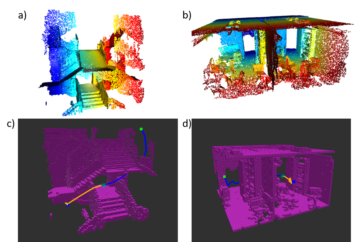
Figure 1: a,b) Point clouds of two real-world environments taken from the 2D-3D-S dataset [1]. c,d) Our method, FlowMPPIProject, controlling a dynamic quadcopter to successfully traverse these two environments. The executed trajectory is shown in blue, and the planned trajectory is shown in orange at an intermediate point in the execution

Previous work has investigated the duality between control and inference [31, 30] and considered both planning and control as inference problems [2, 33, 27]. Several recent papers have considered the finite-horizon stochastic optimal control problem as Bayesian inference, and proposed methods of performing variational inference to approximate the distribution used to sample control sequences [17, 34, 23, 3]. In order to perform variational inference, we must specify a parameterized distribution which is tractable to optimize and sample while also being flexible enough to provide a good approximation of the true distribution over low-cost trajectories, which may exhibit strong environment-dependencies and multimodalities. While more complex representations have been used to represent this distribution [17, 23], these distributions are initially uninformed and must be iteratively improved during deployment. Instead, our proposed method uses a normalizing flow to represent this distribution and we learn the parameters for this model from data.

The advantage of this approach is that it will learn to sample control sequences which are likely to be both goal-directed and collision-free (i.e. low-cost) for the given system. We use the learned distribution as part of our proposed FlowMPPI sampling-based MPC method. This method samples perturbations to a nominal trajectory in both the latent space of the flow and the space of control sequences.

However, as is common in machine learning, a learned model cannot be expected to produce reliable results when its input is radically different from the training data. Because the space of possible environments is very high-dimensional, we cannot hope to generate enough training data to cover the set of possible environments a robot could encounter. This problem compounds when we generate training data in simulation, but the method must be deployed in the real-world (i.e. the sim2real problem). Thus, when deploying this method, the robot may encounter an out-of-distribution (OOD) environment, i.e. one which is radically different from those used in training. In such cases, the learned distribution in unlikely to produce low-cost control sequences.

To generalize our method to OOD environments we present an approach that performs projection on the representation of the environment as part of the MPC process. This projection changes the environment representation to be more in-distribution while also optimizing trajectory quality in the true environment. In essence, this method “hallucinates” an environment that is more familiar to the normalizing flow so that the flow produces reliable results. However, the key insight behind our projection method is that the “hallucinated” environment cannot be arbitrary, it should be constrained to preserve important features of the true environment for the MPC problem at hand. For example, consider a navigation problem for a 2D point robot, shown in Figure 5. If the normalizing flow is trained only on environments consisting of disc-shaped obstacles, an environment with a corridor would be OOD and the flow would be unlikely to produce low-cost trajectories. However, if we morph the environment to approximate the corridor near the robot with disc-shaped obstacles (producing an in-distribution environment), the flow will then produce low-cost samples for MPC.

Our simulation results on a 2D double-integrator and a 3D 12DoF underactuated quadrotor suggest that FlowMPPI with projection outperforms state-of-the-art MPC baselines on both in-distribution and OOD environments, including OOD environments generated from real-world data (Figure 1).

The contributions of this paper are:

• A method to learn an environment-dependent sampling-distribution of low-cost control sequences using a Normalizing Flow

• FlowMPPI - A method that computes a low-cost control sequence by sampling perturbations to a nominal control sequence in both the latent space of the learned normalizing flow and the space of control sequences

• A projection method which changes the environment representation to be more in-distribution while preserving important features of the environment for the MPC problem at hand

• Experiments showing the efficacy of our method on both in-distribution and OOD environments for planar navigation and 12DoF quadrotor tasks, including environments generated from real-world data

II Related Work

II-A Planning & Control as Inference

The connection between control and inference is long established [11, 31, 30]. Attias [2] first framed planning as an inference problem, and proposed a tractable inference algorithm for discrete state and action spaces. Further work has used inference techniques for planning [20, 21] and Stochastic Optimal Control (SOC) [33, 27, 35]. Two widely used sampling based MPC techniques, MPPI [36] and CEM [15], use importance sampling to generate low-cost control sequences, and have strong connections to the inference formulation of SOC which was explored in [34]. Several recent papers have considered the SOC problem as Bayesian inference, and proposed methods of performing Variational Inference (VI) to approximate a posterior over low-cost control sequences [17, 34, 23, 3]. These methods differ in how they represent the variational posterior. VI methods often use an independent Gaussian posterior, known as the mean-field approximation [4]. Okada and Taniguchi [23] represent the control sequence as a Gaussian mixture, and Lambert et al. [17] use a particle representation, extended to handle parameter uncertainty in [3]. These representations allow for greater flexibility in representing complex posteriors. We will similarly use a flexible class of distributions to represent the posterior, but will further make the posterior dependent on the start, goal, and environment. To our knowledge our approach is the first to amortize the cost of computing this posterior by learning a conditional control sequence posterior from a dataset.

II-B Learning sampling distributions for planning

Our work is related to work learning sampling distributions from data for motion planning. Zhang et al. [39] proposed learning a sampling distribution that is trained across multiple environments, but is independent of the environment. Others have proposed learning a sampling distribution which is dependent on the environment, start and goal [10, 26]. These methods were restricted to geometric planning, but Li et al. [18] proposed an approach for kinodynamic planning which learns a generator and discriminator which are used to sample states that are consistent with the dynamics. Recent work by Lai et al. [16] uses a diffeomorphism to learn the sampling distribution; a model that is similar to a normalizing flow. The model we propose will also learn to generate samples conditioned on the start, goal and environment, though in this work we are considering online MPC and not offline planning. Loew et al. [19] uses probabilistic movement primitives (ProMPs) learned from data as the sampling distribution for sample-based trajectory optimization, however the representation of these ProMPs only allows for uni-modal distributions and the sampling distribution is not dependent on the environment. Adaptive and learned importance samplers have been used for sample-based MPC [12, 6], but these methods only consider a single control problem and the learned samplers do not generalize to different goals & environments.

III Problem Statement

This paper focuses on the problem of Finite-horizon Stochastic Optimal Control. We consider a discrete-time system with state $x\in\mathbb{R}^{d_{x}}$ and control $u\in\mathbb{R}^{d_{u}}$ and known transition probability $p(x_{t+1}|x_{t},u_{t})$. We define finite horizon trajectories with horizon $T$ as $\tau=(X,U)$, where $X=\{x_{0},x_{1},...x_{T}\}$ and $U=\{u_{0},u_{1},...u_{T-1}\}$.

Given an initial state $x_{0}$, a goal state $x_{G}$, and a signed-distance field (SDF) of the the environment $E$, our objective is to find $U$ which minimizes the expected cost $E_{p(X|U)}[J(\tau)]$ for a given cost function $J$, where $p(X|U)=\prod^{T-1}_{t=0}p(x_{t+1}|x_{t},u_{t})$. Note that we will use $J$ to mean both the cost on the total trajectory $J(\tau)$ and the cost of an individual state action pair $J(x,u)$. This paper focuses on the problem of collision-free navigation, where $J$ is parameterized by $(x_{G},E)$.

This problem is difficult to solve in the general case because the mapping from environments to collision-free $U$ can be very complex and depends on the dynamics of the system. To aid in finding $U$, we assume access to a dataset $\mathcal{D}=\{E,x_{0},x_{G}\}^{N}$, which will be used to train our method for a given system. We will evaluate our method in terms of its ability to reach the goal without colliding and the cost of the executed trajectory. Moreover, we wish to solve this problem very quickly (i.e. inside a control loop), which limits the amount of computation that can be used.

IV Preliminaries

IV-A Variational Inference for Stochastic Optimal Control

We can reformulate SOC as an inference problem (as in [27, 32, 23, 17]). First, we introduce a binary ‘optimality’ random variable $o$ for a trajectory such that

$$p(o=1|\tau)\propto\exp{(-J(\tau))}$$ (1)

We place a prior $p(U)$ on $U$, resulting in a prior on $\tau$, $p(\tau)=p(X|U)p(U)$ and aim to find posterior distribution $p(\tau|o=1)\propto p(o=1|\tau)p(\tau)$. In general, this posterior is intractable, so we use variational inference to approximate it with a tractable distribution $q(\tau)$ which minimizes the KL-divergence $\mathcal{KL}(q(\tau)||p(\tau|o=1))$ [4]. Since we define the trajectory by selecting the controls, the variational posterior factorizes as $p(X|U)q(U)$. Thus, we must compute an approximate posterior over control sequences. The quantity to be minimized is

$$\begin{split}&\mathcal{KL}\left(q(\tau)||p(\tau|o=1)\right)=\int q(\tau)\log\frac{q(\tau)}{p(\tau|o=1)}d\tau\\ &=\int q(X,U)\log\frac{p(X|U)q(U)p(o=1)}{p(o=1|X,U)p(X|U)p(U)}dXdU\end{split}$$ (2)

Simplifying and omitting terms that do not depend on $\tau$ yields the variational free energy

$$\mathcal{F}=-\mathbb{E}_{q(\tau)}[\log p(o|\tau)+\log p(U)]-\mathcal{H}(q(U))$$ (3)

Where $\mathcal{H}(q(U)$ is the entropy of $q(U)$. Intuitively, we can understand that the first term promotes low-cost trajectories, the second is a regularization on the control, and the entropy term prevents the variational posterior collapsing to a maximum a posteriori (MAP) solution. Note that $\log p(U)$ can be appropriately combined with the cost, i.e. a Gaussian prior can be incorporated as a squared cost on the control, so will be omitted for the rest of the paper.

IV-B Variational Inference with Normalizing flows

Normalizing flows are bijective transformations that can be used to transform a random variable from some base distribution (i.e. a Gaussian) to a more complex distribution [28, 8, 14]. Consider a random variable $z\in\mathbb{R}^{d}$ and with known pdf $p(z)$. Let us define a bijective function $f:\mathbb{R}^{d}\to\mathbb{R}^{d}$ and a random variable $y$ such that $y=f(z)$ and $z=f^{-1}(y)$. According to the change of variable formula, we can define $p(y)$ in terms of $p(z)$ as follows:

$$p(x) =p(z)\left|\det\frac{\partial f}{\partial z}\right|^{-1}$$ (4)

$$\log p(y) =\log p(z)-\log\left|\det\frac{\partial f}{\partial z}\right|$$ (5)

Normalizing flows can be used as a parameterization of the variational posterior [28]. By selecting a base PDF $p(z)$ and a family of parameterized functions $f_{\theta}$, we specify a potentially complex set of possible densities $q_{\theta}(y)$. Suppose that we want to approximate some distribution $p(y)$ with some distribution $q_{\theta}(y)$. The variational objective is to minimize $\mathcal{KL}(q_{\theta}(y)||p(y))$. This is equivalent to:

$$\begin{split}&\mathcal{KL}\left(q_{\theta}(y)||p(y)\right)=\int q_{\theta}(y)\log\frac{q_{\theta}(y)}{p(y)}dx\\ &=\mathbb{E}_{q_{\theta}(y)}[\log q_{\theta}(y)-\log p(y)]\\ &=\mathbb{E}_{p(z)}\left[\log p(z)-\log\left|\det\frac{\partial f_{\theta}}{\partial z}\right|-\log p(y)\right]\end{split}$$ (6)

Thus we can optimize the parameters $\theta$ of the bijective transform $f_{\theta}$ in order to minimize the variational objective. We will use a normalizing flow to represent the control sequence posterior in our method.

V Methods

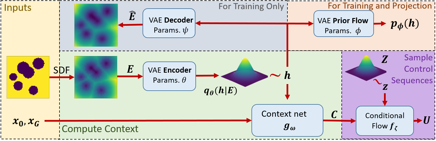
Figure 2: The architecture of our method for sampling control sequences. We take as input initial and goal states $x_{0}$, $x_{G}$, and the environment, converted to a signed distance field $E$. $E$ is input into a VAE to produce a latent distribution $q_{\theta}(h|E)$, which we sample to get the environment embedding $h$. This $h$ is used, along with $x_{0}$ and $x_{G}$ as input to the network $g_{\omega}$ to produce a context vector $C$. $C$, along with a sample from a Gaussian distribution $Z$, is input into the conditional normalizing flow $f_{\zeta}$ to produce a control sequence $U$. During training only, we use a decoder to reconstruct the SDF from $h$ as part of the loss. We also use a normalizing flow prior for the VAE to compute an OOD score for a given $h$, which is necessary to perform projection.

Our proposed architecture for learning an MPC sampling distribution is shown in Figure 2. In this section we first introduce how we represent and learn the control sequence posterior as a Normalizing Flow, and train over a dataset consisting of starts, goals and environments to produce a sampling distribution for control sequences. Next, we show how this sampling distribution can be used to improve MPPI, a sampling based MPC controller. Finally, we describe an approach for adapting the learned sampling distribution to novel environments which are outside the training distribution.

V-A Overview of Learning the Control Sequence Posterior

The control sequence posterior introduced in section IV-A is specific to each MPC problem. Our approach is to use dataset $\mathcal{D}$ to learn a conditional control sequence posterior $q(U|x_{0},x_{G},E)$. We will use a Conditional Normalizing Flow [37] to represent this conditional posterior as $q_{\zeta}(U|C)$. $C$ is the context vector which we compute as follows: First, we input $E$ into the encoder of a Variational Autoencoder (VAE) [13] to produce a distribution over environment embeddings $h$. We then sample from this distribution to produce an $h$. A neural network $g_{\omega}$ then produces $C$ from $(x_{0},x_{G},h)$ (Figure 2). Essentially $C$ is a representation of what is important about the start, goal, and environment for generating low-cost trajectories.

The above models are trained on the dataset $\mathcal{D}$, which consists of randomly sampled starts, goals and simulated environments. To train the system we iteratively generate samples from the control sequence posterior, weigh them by their cost, and perform a gradient step on the parameters of our models to maximize the likelihood of low-cost trajectories.

At inference time, we simply compute $C$ and generate control sequence samples from $q_{\zeta}(U|C)$. Below we describe each component of the method to learn $q_{\zeta}(U|C)$ in detail.

V-B Representing the start, goal and environment as $C$

As discussed, our dataset $\mathcal{D}$ consists of environments, starts and goals. The details of the dataset generation for each task can be found in section VI-A. Since the environment is a high dimensional SDF, we must first compress it to make it computationally tractable to train the control sequence posterior. To encode the environment, we use a VAE with environment embedding $h$. The VAE consists of an encoder $q_{\theta}(h|E)$, which is a Convolutional Neural Network (CNN) that outputs the parameters of a Gaussian. The decoder is a transposed CNN which produces the reconstructed SDF $\hat{E}$ from $h$. The decoder log-likelihood $p_{\psi}(E|h)$ is $||\hat{E}-E||_{2}$, where $\psi$ are the parameters of the decoder CNN. Chen et al. [7] showed that learning a latent prior can improve VAE performance, so we parameterize the latent prior $p_{\phi}(h)$ as a normalizing flow and learn the prior during training. The loss for the VAE is as follows:

$$\begin{split}&\mathcal{L}_{VAE}=\mathbb{E}_{q_{\theta}(h|E)}\left[-\log p_{\psi}(E|h)\right]+\mathcal{KL}(q_{\theta}(h|E)||p_{\phi}(h))\\ &=\mathbb{E}_{q_{\theta}(h|E)}\left[-\log p_{\psi}(E|h)+\log q_{\theta}(h|E)-\log p_{\phi}(h))\right]\end{split}$$ (7)

We then use a Multilayer Perceptron (MLP) network $g_{\omega}$ to generate a context vector $C$ to use in the normalizing flow, via $C=g_{\omega}(x_{0},x_{G},h)$, which has parameters $\omega$.

V-C Learning $q_{\zeta}(U|C)$

We use a conditional normalizing flow parameterized by $\zeta$ to define the conditional variational posterior, i.e. $q_{\zeta}(U|C)$ is defined by $U=f_{\zeta}(Z,C)$ for $Z\sim p(Z)=\mathcal{N}(0,I)$. The variational free energy 3 then becomes:

$$\begin{split}\mathcal{F}=-&\mathbb{E}_{q(\tau)}\left[\log p(o|\tau)\right]+\\ &\mathbb{E}_{p(Z)}\left[\log p(Z)-\log\left|\det\frac{\partial f_{\zeta}(Z,C)}{\partial Z}\right|\right]\end{split}$$ (8)

We can then optimize $\zeta$ to minimize the free energy.

By using a conditional normalizing flow, we are amortizing the cost of computing the posterior across environments. The conditional normalizing flow $U=f_{\zeta}(Z,C)$ is invertible with respect to $Z$, i.e. $Z=f^{-1}(U,C)$. For our conditional Normalizing Flow we use an architecture based on Real-NVP [8] architecture with conditional coupling layers [37], the structure is specified in section VI-C.

Minimizing eq. (8) via gradient descent requires the cost and dynamics to be differentiable. To avoid this, we estimate gradients, using the method in [23]: At each iteration, we sample $R$ control sequences $U_{1..R}$ from $q_{\zeta}(U|C)$ and compute weights

$$w_{i}=\dfrac{q_{\zeta}(U_{i}|C)^{-\beta}p(o|\tau_{i})^{\frac{1}{\alpha}}}{\frac{1}{R}\sum^{R}_{j=1}q_{\zeta}(U_{j}|C)^{-\beta}p(o|\tau_{j})^{\frac{1}{\alpha}}}$$ (9)

where $p(o|\tau)=\mathrm{exp}(-J(\tau))$. These weights represent a trade-off between low-cost and high entropy control sequences controlled by hyperparameters $\alpha$ and $\beta$. The weights and particles $\{U_{1..R},w_{1..R}\}$ effectively approximate a posterior which is closer to the optimal $q(U|C)$. At each iteration of training, we take one gradient step to maximize the likelihood of $U_{1..R}$ weighted by $w_{1..R}$, then resample a new set $U_{1..R}$. The flow training loss for this iteration is

$$\mathcal{L}_{flow}=-\sum^{R}_{i=1}w_{i}\log q_{\zeta}(U_{i}|C)$$ (10)

This process is equivalent to performing mirror descent on the variational free energy, see [23] for a full derivation. In practice, when sampling $U_{1..R}$ from $q_{\zeta}(U|C)$ we add an additional Gaussian perturbation to the samples, decaying the magnitude of the perturbation during training. While this means we are no longer performing gradient descent on $\mathcal{F}$ exactly, we found that this empirically improved exploration during training. To train the parameters of our system we perform the following optimization via stochastic gradient descent:

$$\min_{\theta,\phi,\psi,\omega,\zeta}\mathcal{L}_{flow}+a\mathcal{L}_{VAE}$$ (11)

for scalar $a\geq 0$. We use a combined loss and train end-to-end so that $h$ is explicitly trained to be used to condition the control sequence posterior. We then continue training the control sequence posterior with a fixed VAE with the following optimization:

$$\min_{\omega,\zeta}\mathcal{L}_{flow}$$ (12)

V-D FlowMPPI

We present a method for using the learned control sequence posterior for a control task. Given a $C$ computed from $(x_{0},x_{G},E)$, the control sequence posterior $q_{\zeta}(U|C)$ can be used as a sampling distribution in a sampling-based MPC approach. We propose a method for using the control sequence posterior with MPPI [36], which we term FlowMPPI (Algorithm 1).

MPPI iteratively perturbs a nominal control sequence with Gaussian noise and performs a weighted sum of the perturbations to find a new control sequence. Empirically, we found that standard MPPI is good at performing local optimization on an already-feasible nominal trajectory. On the other hand, the control sequence posterior is able to sample collision-free goal-directed trajectories, but locally improving trajectories with samples is difficult as small changes in the control sequence posterior latent space $Z$ often lead to large differences in the resulting control sequence. As a result, we observed that we obtained trajectories which reached the goal and avoided obstacles with very few samples, however the cost of the best trajectory did not improve much with more iterations of MPPI.

FlowMPPI combines sampling in the latent space $Z$, and sampling perturbations to trajectories to get the advantages of both. For a given sampling budget $K$, we generate half of the samples from perturbing the nominal trajectory as in MPPI, and the other half from sampling from the control sequence posterior. These samples will be combined as in standard MPPI. Since the control sequence posterior is invertible w.r.t $U$, a given nominal trajectory $U$ can be transformed to a latent state $Z$. For the samples from the control sequence posterior, we apply a perturbation cost on the distance of the sampled trajectory from the nominal in latent space. This cost mirrors a similar cost in standard MPPI which penalizes perturbations based on distance to the nominal in the control space.

Algorithm 1 A single step of FlowMPPI, this will run every timestep until task is completed or failure is reached.

Inputs: Cost function $J$, previous nominal trajectory $U$, Context vector $C=g_{\omega}(x_{0},x_{g},h)$, control sequence posterior flow $f_{\zeta}$, MPPI hyperparameters $(\lambda,\Sigma)$, Horizon T, Samples $K$

1:function FlowMPPIStep

2:     $\triangleright$ Perform shift operation on nominal U

3:     for t $\in\{1,...,T-1\}$ do

4:         $U_{t-1}\leftarrow U_{t}$      

5:     $U_{T-1}\sim\mathcal{N}(0,\Sigma)$

6:     $\triangleright$ Map nominal controls to $f_{\zeta}$ latent space

7:     $Z\leftarrow f_{\zeta}^{-1}(U,C)$

8:     $\triangleright$ Generate samples by perturbing nominal U

9:     for k $\in\{1,...,\frac{K}{2}\}$ do

10:         $\epsilon_{U}\sim\mathcal{N}(0,\Sigma)$

11:         $U_{k}\leftarrow U+\epsilon_{U}$

12:         $\tau_{k}\sim p(\tau|U_{k})$ $\triangleright$ Sample trajectory

13:         $S_{k}\leftarrow J(\tau_{k})+\lambda U_{k}\Sigma^{-1}\epsilon_{U}$ $\triangleright$ Compute cost      

14:     $\triangleright$ Generate samples from control sequence posterior

15:     for k $\in\{\frac{K}{2}+1,...,K\}$ do

16:         $\epsilon_{Z}\sim\mathcal{N}(0,I)$

17:         $U_{k}\leftarrow f_{\zeta}(\epsilon_{Z},C)$

18:         $\tau_{k}\sim p(\tau|U_{k})$ $\triangleright$ Sample trajectory

19:         $S_{k}\leftarrow J(\tau_{k})+\lambda\epsilon_{Z}(Z-\epsilon_{Z})$ $\triangleright$ Compute cost      

20:     $\triangleright$ Compute new nominal U

21:     $\beta\leftarrow\min_{k}S_{k}$

22:     $\eta=\sum^{K}_{k=1}\exp(-\frac{1}{\lambda}(S_{k}-\beta))$

23:     for k $\in\{1,...,K\}$ do

24:         $w_{k}\leftarrow\frac{1}{\eta}\exp(-\frac{1}{\lambda}(S_{k}-\beta))$      

25:     $U\leftarrow\sum^{K}_{k=1}w_{k}U_{k}$

26:     return $U$

V-E Generalizing to OOD Environments

A novel environment can be OOD for the control sequence posterior and result in poor performance. We present an approach where we project the OOD environment embedding $h$ in-distribution in order to produce low-cost trajectories when it is used as part of the input to $f_{\zeta}$. The intuition behind this approach is that our goal is to sample low-cost trajectories in the current environment. Given that $f_{\zeta}$ will have been trained over a diverse set of environments, if we can find an in-distribution environment that would elicit similar low-cost trajectories, then we can use this environment as a proxy for the actual environment when sampling from the flow. Thus we avoid the problem of samples from the control sequence posterior being unreliable when the input is OOD.

In order to do this projection, we first need to quantify how far out-of-distribution a given environment is. Once we have such an OOD score, we will find a proxy environment embedding $\hat{h}$ by optimizing the score, while also regularizing to encourage low-cost trajectories. For the OOD score, we use the VAE we have discussed in section V-B. VAEs and other deep latent variable models have been used to detect OOD data in prior work [9, 38, 22], however these methods are typically based on evaluating the likelihood of an input, in our case $p(E)$. For VAEs this requires reconstruction. We would like to avoid using reconstruction in our OOD score for two reasons. First, reconstruction, particularly of a 3D SDF, adds additional computation cost and we would like to evaluate the OOD score in an online control loop. Second, optimizing an OOD score based on reconstruction would drive us to find an environment embedding proxy which is able to approximately reconstruct the entire environment. This makes the problem more difficult than is necessary, as we do not need $\hat{h}$ to accurately represent the entire environment, only to elicit low-cost trajectories from the control sequence posterior.

To determine how close $h$ is to being in-distribution, we use the following OOD score:

$$\mathcal{L}_{OOD}(h)=-\log p_{\phi}(h)$$ (13)

where $p_{\phi}(h)$ is the learned flow prior for the VAE. The intuition for using this as an OOD score is that this term is minimized for the dataset in $\mathcal{L}_{VAE}$, so we should expect it to be lower for in-distribution data. Using a learned prior was shown to improve density estimation over a Gaussian prior [7] and we found the learned prior yielded much better OOD detection than using a Gaussian prior, which is the standard VAE prior (see Figure 3).

We can perform gradient descent on $\mathcal{L}_{OOD}$ to find $\hat{h}$, thus projecting the environment to be in-distribution. Note that without regularization this process will converge to a nearby maximum likelihood solution, which may lose key features of the current environment. Since our aim is to sample low-cost trajectories from the control sequence posterior, we use $\mathcal{L}_{flow}$ as a regularizer for this gradient descent. Our intuition here is that in order to generate low-cost trajectories in the true environment, the projected environment embedding should preserve important features of the environment relevant for that particular planning query. The new environment embedding is then given by

$$\hat{h}=\arg\min_{h}\>b\mathcal{L}_{OOD}+\mathcal{L}_{flow}$$ (14)

for scalar $b>0$. We project $h$ to $\hat{h}$ by minimizing the above by gradient descent. This step is incorporated into FlowMPPI in a version of our method FlowMPPIProject. This version of our method will perform $M$ steps of gradient descent on the above combined loss at initialization, followed by a single step at each iteration of FlowMPPIProject. The algorithm for projection is shown in algorithm 4 in appendix -E.

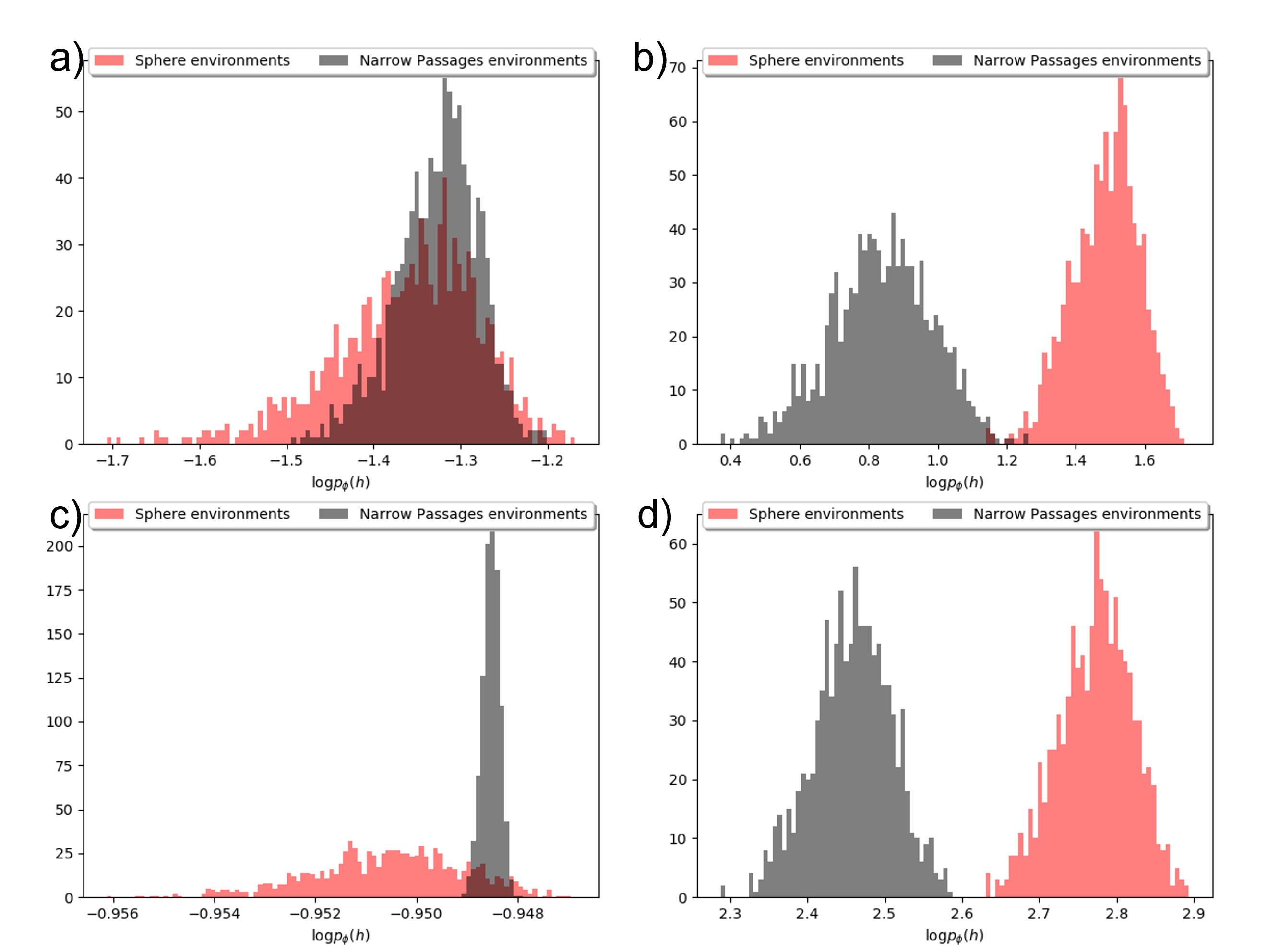
Figure 3: Comparison of our OOD scores with using a VAE with a standard Gaussian prior for in-distribution (red) and out-of-distribution (grey) simulated environments. a) planar navigation using a Gaussian prior, b) planar navigation using a Normalizing flow prior, c) 12DoF quadrotor using a Gaussian prior, d) 12DoF quadrotor using a Normalizing flow prior, These scores are computed by sampling $h$ from $q_{\theta}(h|E)$ and evaluating $\log p_{\phi}(h)$. The score is normalized by the dimensionality of $h$. We see that our method, shown in (b) and (d), achieves a clear separation between in-distribution and out-of-distribution environments in both cases.

VI Evaluation

In this section, we will evaluate our proposed approaches FlowMPPI & FlowMPPIProject on two simulated systems; a 2D point robot and a 3D 12DoF quadrotor. For each system, we will train the flow on a dataset of starts, goals and environments and evaluate the performance on environments drawn from the same distribution. In addition, for each system we will test on novel environments that are radically different from those used for training and evaluate the generalization of our approach and the ability of FlowMPPIProject to adapt to these OOD environments. For the 12DoF quadrotor system, we additionally evaluate our method in simulation on two environments generated from real-world data from the 2D-3D-S dataset [1], where our goal is to evaluate if the control sequence posterior, trained on simulated environments, can adapt to real-world environments.

For our novel environments, we select environments which are difficult for sampling-based MPC techniques. We will use the terms “in-distribution” and “out-of distribution” for environments for the rest of this section, but note that these terms are relative to the set of environments which we use to train our method. Being out-of-distribution has no bearing on the non-learning based baselines. The performance of non-learning sampling-based MPC algorithms depends only on the given environment, not its relation to other environments.

VI-A Systems & Environments

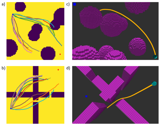
Figure 4: Examples of our ’in-distribution’ environments (top) and ’out-of-distribution’ environments (bottom). a) The sphere environment for the planar navigation task, showing sampled trajectories from the flow. b) The narrow passages environment for planar navigation, we see that the samples from the flow are goal orientated and generally toward the passages, but most are generally not collision free. c) The sphere environment for the 12DoF quadrotor. d) The narrow passages environment for the 12DoF quadrotor

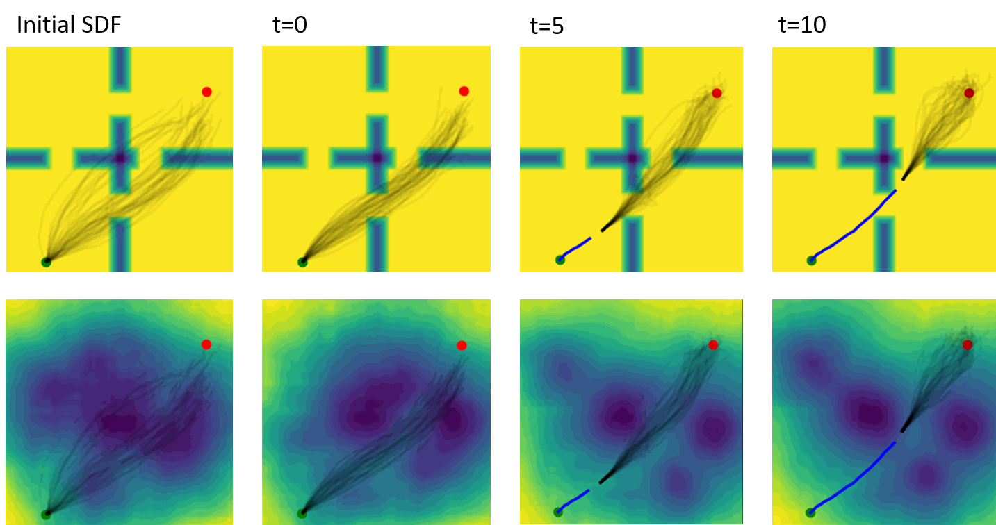
Figure 5: The projection process visualized for the planar navigation task. We visualize the projected environment embedding using the VAE decoder. Note that decoding $h$ is only used for training the VAE and visualization, it is not necessary for projection. The top shows the environment and sampled trajectories from $q_{\zeta}(U|C)$. The bottom shows the same samples overlaid on a reconstruction of projected environment embedding $\hat{h}$. On the left, the initial SDF is very poor. As the task progresses, the iterative projection results in an SDF that resembles the training environment more. The environment embedding encodes obstacles that result in a trajectory which traverses the narrow passage. Notice however, that regions that are not relevant for this planning task, such as the top left corner, do not need to accurately represent the environment.

In this section we will introduce the systems and the environments we use for evaluation. For all systems and environments, a task is considered a failure if there is a collision or if the system does not reach the goal region within a timeout of 100 timesteps. The cost function for both systems is given by $J(\tau)=100d_{G}(x_{T})+\sum^{T-1}_{t=1}10d_{G}(x_{t})_{2}+\sum^{T}_{t=1}10000D(x_{t})$, where $T$ is the MPC horizon, $d_{G}$ is a distance to goal function, and $D$ is an indicator function which is 1 if $x_{t}$ is in collision and 0 otherwise. For all of our experiments, the control horizon $T=40$. We use a Gaussian prior over controls is $p(U)=\mathcal{N}(0,\sigma^{2}I)$ which induces a cost on the squared magnitude of the actions. For all of our experiments the dynamics are deterministic. Further details of the generation of training data can be found in appendix -C.

VI-A1 Planar Navigation

The robot in the planar navigation task is a point robot with double-integrator dynamics. The goal is to perform navigation in an environment cluttered with obstacles. The state and control dimensionality are 4 and 2, respectively. The environment is represented as a $64\times 64$ SDF. Examples of the training and evaluation environments are shown in Figure 4 (a & b). The training environments consist disc-shaped obstacles, where the size, location and number of obstacles is randomized. The out-of-distribution environment consists of four rooms, with narrow passages randomly generated between them. The location of the passages is randomized for each OOD environment. The distance to goal function is $d_{G}(x)=||x-x_{G}||_{2}$. The goal region for this task is given by $\mathcal{X}_{G}=\{x:||x-x_{G}||_{2}<0.1$}. The dynamics for this system are shown in appendix -C2.

VI-A2 3D 12DoF Quadrotor

This system is a 3D 12DoF underactuated quadrotor with the shape of a short cylinder. It has state and control dimensionality of 12 and 4, respectively. As with the planar navigation task, the goal is to perform navigation in a cluttered environment. Examples of the training and evaluation environments are shown in Figure 4 (c & d). The training environment consists of spherical obstacles of random size, location, and number, and the out-of-distribution environment of four rooms separated by randomly generated narrow passages. The environment is represented as a $64\times 64\times 64$ SDF. The goal region is specified as a 3D position $p_{G}$. The distance to goal function is $d_{G}(x)=||Ax-p_{G}||_{2}+0.01||Bx||_{2}$ where $A$ selects the position components from the state $x$, and $B$ selects the angular velocity components. The goal region is $\mathcal{X}_{G}=\{x:d_{G}(x)<0.3$}. We also tested in two simulation environments generated from real-world data (shown in 1). The dynamics for this system are shown in appendix -C3.

VI-B OOD Score and Projection

To confirm the efficacy of our OOD score, we computed this score for the training and OOD environments for each system above. Figure 3 shows that this score is clearly able to distinguish in-distribution environment embeddings from OOD ones. To show the necessity of using both the OOD score and the regularization in projection, we perform an ablation on these two components in appendix -F for the quadrotor system.

VI-C Network Architectures

For both the control sequence posterior flow $f_{\zeta}$ and the VAE prior $p_{\phi}(h)$ we use an architecture based on Real-NVP [8]. For the VAE prior $p_{\phi}(h)$ we use a flow depth of 4, while for the control sampling flow $f_{\zeta}$ we use a flow depth of 10. For the control sampling flow we use the conditional coupling layers from [37]. For the VAE encoder we use four CNN layers with a kernel of 3 and a stride of 2, followed by a fully connected layer. For the VAE decoder we used a fully connected layer followed by four transposed CNN layers. For the 3D case we use 3D convolutions. The dimensionality of both $h$ and $C$ was $64$ for the planar navigation environments $256$ for 3D 12DoF quadrotor environments. $g_{\omega}$ was defined as an MLP with a single hidden layer of size $256$. For nonlinear activations we used ReLU throughout.

VI-D Training & Data

For training, we use $10000$ randomly generated environments for planar navigation task, and $20000$ for the 3D 12DoF quadrotor task. At each epoch, for each environment, we randomly select one of $100$ start and goal pairs. We train the control sequence posterior flow $f_{\zeta}$, the VAE parameters ($\theta,\phi,\psi$) and the context MLP $g_{\omega}$ end-to-end using Adam for $1000$ epochs with a learning rate of $1e^{-3}$, with a decay rate of $0.9$ every 50 epochs. After 100 epochs, we freeze the VAE and do not continue training with $\mathcal{L_{VAE}}$. This is primarily because the VAE converges quickly and training proceeds more quickly without reconstruction. When training the VAE we divide the loss by the total dimensionality of the SDF and use $a=5$. For every environment for the flow training, hyperparameters we use $\beta=1$ and we linearly increase $\alpha$ from $1$ to $500$ during training. Empirically we found that low initial $\alpha$ was required for the flow to learn to generate goal-directed trajectories early on during training, and that increasing $\alpha$ later during training increases the diversity of the flow sampling distribution. A more details list of training hyperparameters can be found in appendix 6

VI-E Baselines

For our baselines we use several state-of-the-art sampling-based MPC methods: MPPI [36], Stein Variational MPC (SVMPC) [17] and improved CEM (iCEM) [24]. MPPI uses a Gaussian distribution as the sampling distribution, iCEM uses colored noise, and SVMPC uses a mixture of Gaussians. For each baseline, we tune the hyperparameters to get the best performance based on the training environments, and maintain these hyperparameters when switching to the out-of-distribution environments. When evaluating our two proposed methods and the baselines, each method is given the same sampling budget per timestep. This means that for methods that require multiple iterations per timestep, the sampling budget is distributed across the iterations. A more detailed list of the hyperparameters for each controller can be found in appendix -D. Evaluating $\mathcal{L}_{flow}$ during projection requires sampling and evaluating control sequences. When we consider the sampling budget of different algorithms in evaluation, we will include these samples. FlowMPPIProject uses half of the allowed sampling budget during the project step, and the other half for the FlowMPPI control algorithm. While it does take longer to sample from the flow than from the distributions in the baselines, we observe that the cost of evaluating control sequences dominates over the cost of sampling. For example, for the 3D 12DoF quadrotor system, sampling 1024 control sequences from the flow and evaluating the cost of these control sequences takes on average $9$ms and $80$ms, respectively on an i7-8700K CPU and Nvidia 1080 Ti GPU.

		In-Distribution		Out-of Distribution
		K=512		K=256		K=512		K=1024
System	Controller	Success	Cost	Success	Cost	Success	Cost	Success	Cost
Planar Navigation	MPPI	0.89	1925	0.19	3180	0.29	2948	0.36	2840
	SVMPC	0.97	1523	0.18	3032	0.22	2727	0.25	2666
	iCEM	0.97	1531	0.46	2467	0.59	2145	0.62	2127
	FlowMPPI	0.99	1705	0.62	2731	0.75	2155	0.84	2104
	FlowMPPIProject	0.99	1737	0.65	2690	0.77	2155	0.87	2059
12DoF Quadrotor	MPPI	0.57	3589	0.05	4809	0.11	4724	0.27	4351
	SVMPC	0.55	3745	0.11	5588	0.21	4947	0.44	4486
	iCEM	0.96	2724	0.35	4388	0.47	4157	0.63	3795
	FlowMPPI	0.92	2595	0.56	3805	0.72	3601	0.84	3421
	FlowMPPIProject	0.98	2437	0.71	3688	0.83	3443	0.93	3200

TABLE I: Comparison of methods on 100 randomly generated environments, starts and goals for both in distribution and out-of-distribution training environments. Performance on out-of-distribution environments is evaluated for three different sampling budgets.

	Rooms Environment		Stairway Environment
Method	Success	Cost	Success	Cost
MPPI	0.83	3111	0.32	3019
SVMPC	0.68	7556	0.49	2770
iCEM	0.92	2412	0.58	2623
FlowMPPI	0.87	2375	0.5	2463
FlowMPPIProject	0.97	1972	0.85	1745

TABLE II: Comparison of methods for the 3D 12DoF quadrotor navigation task with two environments generated from real-world data. The rooms environment is shown in figure 4 (b) and the stairway environment is shown in figure 4 (a). We evaluate on 100 randomly sampled starts and goals in each environment.

VI-F Results

The results comparing our MPC methods to baselines are shown in Tables I and II. For the planar navigation case, we see that FlowMPPI and FlowMPPIProject are competitive with the baselines on the training environments. Our method reaches the goal region more often, while attaining slightly higher average cost. For the out-of-distribution environments, our method reaches the goal significantly more often. For example, with a sampling budget of $256$, the success rates for FlowMPPIProject is $0.65$ and increases to $0.87$ for a sampling budget of 1024. The next closest baseline, iCEM, has successes rates of $0.46$ and $0.62$ for sampling budgets of $256$ and $1024$, respectively. The projection process for the planar navigation task is visualized for an OOD environment in Figure 5.

We observed during this experiment that when iCEM and SVMPC are able to generate a trajectory which reaches the goal region, they are able to locally optimize this trajectory better than FlowMPPI variants, while FlowMPPI is better able to generate sub-optimal trajectories to the goal region.

For the quadrotor system, FlowMPPIProject outperforms all other methods in both cost and success rate across all environments and sampling budgets. With a sampling budget of $256$, FlowMPPIProject attains a $71\%$ success rate compared to $35\%$ by iCEM and $11\%$ by SVMPC for OOD environments. For a sampling budget of $1024$ the success rate of FlowMPPIproject rises to $93\%$ vs. $63\%$ for iCEM. The dynamics of this task make it much more difficult, particularly because stabilizing around the goal is non-trivial. We found that the baselines struggled to find trajectories which both reached and stabilized to the goal, and thus were more susceptible to becoming stuck in local minima.

Table II shows the results when evaluating our method in simulation in two environments generated from real-world data. FlowMPPIProject outperforms all baselines in cost & success rate, despite only being trained on simulated environments consisting of large spherical obstacles. For the challenging stairway environment, FlowMPPIProject achieves $85\%$ success, while the next closest baseline, iCEM, has $58\%$ success. FlowMPPI achieves only $50\%$ success rate for this task, highlighting the importance of projection for real-world environments.

VII Conclusion

In this paper we have presented a framework for using a Conditional Normalizing Flow to learn a control sequence sampling distribution for MPC based on the formulation of MPC as Variational Inference. The control sequence posterior samples control sequences which result in low-cost trajectories that avoid collision. We have shown how this control sequence posterior can be used in a sampling-based MPC method FlowMPPI. We have also proposed a method for adapting this control sequence posterior to OOD environments by projecting the representation of the environment to be in-distribution, essentially “hallucinating” an in-distribution environment which elicits low-cost trajectories from the control sequence posterior. We have demonstrated that our proposed MPC methods FlowMPPI and FlowMPPIProject offer large improvements over baselines in difficult environments, and that by performing the environment projection we can successfully transfer a control sequence posterior learned with simulated environments to environments generated from real-world data.

-A Variational Inference for Finite-Horizon Stochastic Optimal Control

The variational posterior over trajectories is defined by the dynamics and the variational posterior over actions:

$$\begin{split}q(\tau|x_{0})&=q(X,U|x_{0})\\ &=p(X|U,x_{0})q(U)\\ &=q(U)\prod^{T}_{t=0}p(x_{t+1}|x_{t},u_{t})\end{split}$$ (15)

We will omit the dependence on the initial state $x_{0}$ for convenience.

$$\begin{split}&\mathcal{KL}\left(q(\tau)||p(\tau|o=1)\right)=\int q(\tau)\log\frac{q(\tau)}{p(\tau|o=1)}d\tau\\ &=\int q(X,U)\log\frac{p(X|U)q(U)p(o=1)}{p(o=1|X,U)p(X|U)p(U)}dXdU\end{split}$$ (16)

Since $p(o=1)$ on the numerator does not depend on U, when we minimize the above divergence it can be dropped. The result is minimizing the below quantity, the variational free energy $\mathcal{F}$.

$$\mathcal{F} =\int q(X,U)\log\frac{q(U)}{p(o=1|X,U)p(U)}dXdU$$ (17)

$$\begin{split}&=-\mathbb{E}_{q(X,U)}\left[\log p(o|X,U)+\log p(U)-\log q(U)\right]\\ \end{split}$$ (18)

$$=\mathbb{E}_{q(X,U)}\left[J(X,U)\right]+\mathcal{KL}(q(U)||p(U))$$ (19)

$$=\mathbb{E}_{q(X,U)}\left[\hat{J}(X,U)+\log q(U)\right]$$ (20)

For the last two expressions we have used our formulation that the $p(o=1|X,U)=\exp(-J(X,U))$, where $J$ is the trajectory cost, and we have incorporated the deviation from the prior into the cost function. For example, a zero-mean Gaussian prior on the controls can be equivalently expressed as a squared cost on the magnitude of the controls.

-B Training & Architecture Details

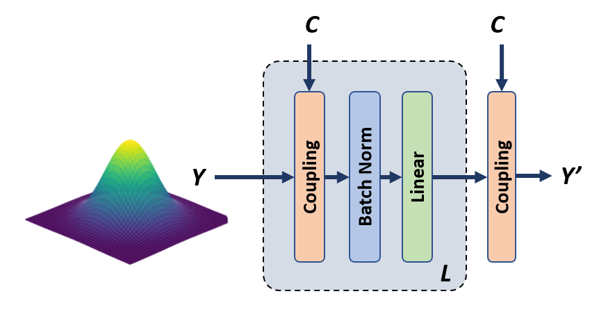
Figure 6: The architecture for both the prior flow and the control sequence posterior flow, based on [8] and [37], showing a mapping from arbitrary Y to Y’. Each flow consists of L chained transformation blocks. A transformation block consists of a conditional coupling layer, a batch norm layer, and a linear layer. There is a final conditional coupling layer on the output. For the vae prior, there is no context therefore we use standard coupling layers and not conditional coupling layers.

Variable	Planar Navigation	3D 12DoF Quadrotor
control peturbation $\Sigma_{e}$	$1-\dfrac{\text{epoch}}{\#\text{epochs}}$
$\alpha$	$500\dfrac{\text{epoch}}{\#\text{epochs}}$
$\beta$	1	1
$\#$ epochs	1000	1000
Initial learning rate	$1\times 10^{-3}$	$1\times 10^{-3}$
Learning rate decay	$0.9$ every 50 epochs
$\#$ Training environments	10000	20000
$\#$ $(x_{0},x_{G})$ per training env.	100	100
$h$ dim	64	256
$a$	5	5
$b$	$\dfrac{1}{64}$	$\frac{1}{1024}$
VAE training epochs	100	100
$p_{\phi}(h)$ flow depth L	4	4
$f_{\zeta}$ flow depth L	10	10

TABLE III: Training and architecture hyperparameters for each experiment.

-B1 Hyperparameter Tuning

There are several hyperparameters to tune in our approach. The scalar $a$ in equation 11 was tuned so that $a\mathcal{L}_{VAE}$ and $\mathcal{L}_{flow}$ were of approximately similar magnitude. The scalar $b$ in equation 14 was selected to be equal to the dimensionality of the SDF observation divided by the dimensionality of the latent environment embedding. This value was chosen initially to make the projection loss similar across the quadcopter and the double integrator, and we found this automatic tuning worked well in practice. Hyperparameters $\alpha,\beta$ together control the trade-off between entropy and optimality. We kept $\beta$ fixed and tuned only $\alpha$. To tune $\alpha$, for each experiment we performed a grid search and selected the value of $\alpha$ that resulted in the best performance in the training environment when used with FlowMPPI.

-C Environment details

The environments are $4m\times 4m$, and generated as occupancy grids, from which we compute the SDF. For each training environment, we randomly sample 100 start & goal pairs such that they are always collision free, and within the bounds of the voxel grid. We sample start velocities from a Normal distribution, and set the goal velocity to be zero. During evaluation, for both the in-distribution and out-of-distribution environments, we sample $100$ start, goal and environment tuples and evaluate all methods on these tuples. The exception to this is the real-world environments, where we keep the environments fixed and sample $100$ start and goal pairs per real-world environment and evaluate all methods on these pairs. To ensure the navigation problem is non-trivial, we sample starts and goals that are at least $4m$ away.

-C1 Real-world environments

The two real world environments are taken from area 3 from the 2D-3D-S dataset [1]. To generate the two environments, we used the 3D mesh from the dataset and defined a subset of the area to be the environment. We then generated an occupancy grid by densely sampling the mesh, which we then used to compute the SDF.

-C2 Planar Navigation

The dynamics for the planar navigation system are

$$\begin{bmatrix}x\\ y\\ \dot{x}\\ \dot{y}\end{bmatrix}_{t+1}=\begin{bmatrix}1&0&\Delta t&0\\ 0&1&0&\Delta t\\ 0&0&0.95&0\\ 0&0&0&0.95\end{bmatrix}\begin{bmatrix}x\\ y\\ \dot{x}\\ \dot{y}\end{bmatrix}_{t}+\begin{bmatrix}0&0\\ 0&0\\ \Delta t&0\\ 0&\Delta t\\ \end{bmatrix}\mathbf{u}$$ (21)

-C3 12DoF Quadrotor

The dynamics for the 12DoF quadrotor are from Sabatino [29] and are given by

$$\begin{bmatrix}x\\ y\\ z\\ p\\ q\\ r\\ \dot{x}\\ \dot{y}\\ \dot{z}\\ \dot{p}\\ \dot{q}\\ \dot{r}\\ \end{bmatrix}_{t+1}=\begin{bmatrix}x\\ y\\ z\\ p\\ q\\ r\\ \dot{x}\\ \dot{y}\\ \dot{z}\\ \dot{p}\\ \dot{q}\\ \dot{r}\\ \end{bmatrix}_{t}+\Delta t\begin{bmatrix}\dot{x}\\ \dot{y}\\ \dot{z}\\ \dot{p}+\dot{q}s(p)t(q)+\dot{r}c(p)t(q)\\ \dot{q}c(p)-\dot{r}s\dot{p}\\ \dot{q}\dfrac{s(p)}{c(q)}+\dot{r}\dfrac{c(p))}{c(q)}\\ -(s(p)s(r)+c(r)c(p)s(q))K\frac{u_{1}}{m}\\ -(c(r)s(p)-c(p)s(r)s(q))K\frac{u_{1}}{m}\\ g-c(p)s(q))K\frac{u_{1}}{m}\\ \frac{(I_{y}-I_{z})\dot{q}\dot{r}+Ku_{2}}{I_{x}}\\ \frac{(I_{z}-I_{x})\dot{p}\dot{r}+Ku_{3}}{I_{y}}\\ \frac{(I_{x}-I_{y})\dot{p}\dot{q}+Ku_{4}}{I_{z}}\\ \end{bmatrix}_{t}$$ (22)

Where $c(p),s(p),t(p)$ are $\cos,\sin,\tan$ functions respectively. We use a parameters $m=1,I_{x}=0.5,I_{y}=0.1,I_{z}=0.3,K=5,g=-9.81$. The quadrotor geometry is modeled as a cylinder with radius $0.1m$ and height $0.05m$.

-D Controller details

Variable	Planar Navigation	12DoF Quadrotor
Control Horizon $H$	40	40
Trial length $T$	100	100
Control prior $\sigma$	1	4
Dynamics $\Delta t$	0.05	0.025

TABLE IV: Controller agnostic parameters used for the evaluations

.

Controller	Variable	Planar Navigation	12DoF Quadrotor
MPPI	$\lambda$	1	1
	$\Sigma$	0.9	0.5
	iterations	1	4
SVMPC	$\Sigma$	1	0.5
	$\#$ particles	4	4
	Learning rate	1	0.5
	iterations	4	4
	warm-up iterations	25	25
iCEM	$\Sigma$	0.75	0.5
	noise parameter	2.5	3
	$\%$ elites	0.1	0.1
	$\%$ kept elites	0.3	0.5
	iterations	4	4
	momentum	0.1	0.1
FlowMPPI	$\lambda$	1	1
	$\Sigma$	1	0.75
	iterations	1	2
	$M$	10	10
	Proj. learn. rate	$1\times 10^{-2}$	1$\times 10^{-2}$

TABLE V: Controller hyperparameters used for the experiments for both our proposed method and the baselines.

-E Algorithms

Algorithm 2 Sample from Control Sequence Posterior with Perturbation

1:function SamplePertU($C,\Sigma_{\epsilon},K$)

2:     for i $\in\{k,...,K\}$ do

3:         $Z_{k}\sim\mathcal{N}(0,I)$

4:         $\epsilon_{k}\sim\mathcal{N}(0,\Sigma_{\epsilon})$

5:         $U_{k}\leftarrow f_{\zeta}(Z_{k},C)+\epsilon_{k}$

6:         $\hat{Z}_{k}\leftarrow f_{\zeta}^{-1}(U_{k},C)$

7:         $q_{\zeta}(U_{k}|C)\leftarrow\text{from $\hat{Z}_{k}$ via eq. (\ref{background:flow_ll}})$      

8:     return $\{U_{k},q_{\zeta}(U_{k}|C)\}^{K}_{k=1}$

Algorithm 3 Flow Training

Inputs: N iterations, K samples, $\Theta^{1}=\{\theta^{1},\psi^{1},\phi^{1},\omega^{1},\zeta^{1}\}$ initial parameters, control perturbation covariance $\Sigma_{\epsilon}$, learning rate $\eta$, loss hyperparameters $(\alpha,\beta)$

1:for n $\in\{1,...,N\}$ do

2:     $h\leftarrow q_{\theta}(h|E)$

3:     $\hat{E}\leftarrow p_{\psi}(E|h)$

4:     Compute $\log p_{\phi}(h)$ via eq. (5)

5:     Compute $\mathcal{L}_{VAE}$

6:     $C\leftarrow g_{\omega}(x_{0},x_{G},h)$

7:     $\{U_{k},q_{\zeta}(U_{k}|C)\}^{K}_{k=1}\leftarrow\textsc{SamplePertU}(C,\Sigma_{\epsilon},K)$

8:     $\mathcal{L}\leftarrow\mathcal{L}_{VAE}$

9:     for k $\in\{1,...,K\}$ do

10:         $w_{k}\leftarrow\text{from $(\{U_{i},\log q_{\zeta}(U_{i}|C)\}^{K}_{i=1},\alpha,\beta\})$ via (\ref{eq:update_law}})$

11:         $\mathcal{L}\leftarrow\mathcal{L}-w_{k}\cdot\log q_{\zeta}(U_{k}|C)$      

12:     $\Theta^{n+1}\leftarrow\Theta^{n}-\eta\frac{\partial\mathcal{L}}{\partial\Theta}$

Algorithm 4 Projection

Inputs: N iterations, K samples, $\theta,\phi,\omega,\zeta$ parameters, control perturbation covariance $\Sigma_{\epsilon}$, learning rate $\eta$, loss hyperparameters $(\alpha,\beta)$

1:$h^{1}\leftarrow q_{\theta}(h|E)$

2:for n $\in\{1,...,N\}$ do

3:     Compute $\log p_{\phi}(h^{n})$ via eq. (5)

4:     $C\leftarrow g_{\omega}(x_{0},x_{G},h^{n})$

5:     $\{U_{k},q_{\zeta}(U_{k}|C)\}^{K}_{k=1}\leftarrow\textsc{SamplePertU}(C,\Sigma_{\epsilon},K)$

6:     $\mathcal{L}\leftarrow-p_{\phi}(h^{n})$

7:     for k $\in\{1,...,K\}$ do

8:         $w_{k}\leftarrow\text{from $(\{U_{i},\log q_{\zeta}(U_{i}|C)\}^{K}_{i=1},\alpha,\beta\})$ via (\ref{eq:update_law}})$

9:         $\mathcal{L}\leftarrow\mathcal{L}-w_{k}\cdot\log q_{\zeta}(U_{k}|C)$      

10:     $h^{n+1}\leftarrow h^{n}-\eta\frac{\partial\mathcal{L}}{\partial h}$

-F Additional Results

	K=256		K=512		K=1024
Projection loss	Success	Cost	Success	Cost	Success	Cost
$\mathcal{L}_{OOD}+\mathcal{L}_{flow}$	0.71	3688	0.83	3443	0.93	3200
$\mathcal{L}_{OOD}$	0.52	3859	0.63	3704	0.89	3371
$\mathcal{L}_{flow}$	0.6	3758	0.72	3489	0.87	3226

TABLE VI: Ablation of the different loss terms in FlowMPPIProject for different sampling budgets for the 12DoF quadrotor out-of-distribution environment

References

- Armeni et al. [2017] I. Armeni, A. Sax, A. R. Zamir, and S. Savarese. Joint 2D-3D-Semantic Data for Indoor Scene Understanding. ArXiv e-prints, 2017.
- Attias [2003] Hagai Attias. Planning by Probabilistic Inference. In AISTATS, 2003.
- Barcelos et al. [2021] Lucas Barcelos, Alexander Lambert, Rafael Oliveira, Paulo Borges, Byron Boots, and Fabio Ramos. Dual Online Stein Variational Inference for Control and Dynamics. In RSS, 2021.
- Blei et al. [2017] David M. Blei, Alp Kucukelbir, and Jon D. McAuliffe. Variational inference: A review for statisticians. Journal of the American Statistical Association, 2017.
- Brasseur et al. [2015] Camille Brasseur, Alexander Sherikov, Cyrille Collette, Dimitar Dimitrov, and Pierre-Brice Wieber. A robust linear mpc approach to online generation of 3d biped walking motion. In Humanoids, 2015.
- Carius et al. [2022] Jan Carius, René Ranftl, Farbod Farshidian, and Marco Hutter. Constrained stochastic optimal control with learned importance sampling: A path integral approach. IJRR, 2022.
- Chen et al. [2017] Xi Chen, Diederik P. Kingma, Tim Salimans, Yan Duan, Prafulla Dhariwal, John Schulman, Ilya Sutskever, and Pieter Abbeel. Variational lossy autoencoder. In ICLR, 2017.
- Dinh et al. [2017] Laurent Dinh, Jascha Sohl-Dickstein, and Samy Bengio. Density estimation using real NVP. In ICLR, 2017.
- Feng et al. [2021] Yeli Feng, Daniel Jun Xian Ng, and Arvind Easwaran. Improving variational autoencoder based out-of-distribution detection for embedded real-time applications. ACM Trans. Embed. Comput. Syst., 2021.
- Ichter et al. [2018] Brian Ichter, James Harrison, and Marco Pavone. Learning sampling distributions for robot motion planning. In ICRA, pages 7087–7094, 05 2018.
- Kalman [1960] R. E. Kalman. A new approach to linear filtering and prediction problems. Journal of Basic Engineering, 1960.
- Kappen and Ruiz [2016] HJ Kappen and HC Ruiz. Adaptive importance sampling for control and inference. Journal of Statistical Physics, 2016.
- Kingma and Welling [2014] Diederik P. Kingma and Max Welling. Auto-encoding variational bayes. In Yoshua Bengio and Yann LeCun, editors, ICLR, 2014.
- Kingma and Dhariwal [2018] Durk P Kingma and Prafulla Dhariwal. Glow: Generative flow with invertible 1x1 convolutions. In NeurIPS, 2018.
- Kobilarov [2012] Marin Kobilarov. Cross-entropy motion planning. IJRR, 2012.
- Lai et al. [2021] Tin Lai, Weiming Zhi, Tucker Hermans, and Fabio Ramos. Parallelised diffeomorphic sampling-based motion planning. In CoRL, 2021.
- Lambert et al. [2020] Alexander Lambert, Adam Fishman, Dieter Fox, Byron Boots, and Fabio Ramos. Stein Variational Model Predictive Control. In CoRL, 2020.
- Li et al. [2021] Linjun Li, Yinglong Miao, Ahmed H. Qureshi, and Michael C. Yip. Mpc-mpnet: Model-predictive motion planning networks for fast, near-optimal planning under kinodynamic constraints, 2021.
- Loew et al. [2021] Tobias Loew, Tirthankar Bandyopadhyay, Jason Williams, and Paulo Borges. PROMPT: Probabilistic Motion Primitives based Trajectory Planning. In RSS, 2021.
- Mukadam et al. [2016] Mustafa Mukadam, Xinyan Yan, and Byron Boots. Gaussian process motion planning. In ICRA, 2016.
- Mukadam et al. [2018] Mustafa Mukadam, Jing Dong, Xinyan Yan, Frank Dellaert, and Byron Boots. Continuous-time gaussian process motion planning via probabilistic inference. IJRR, 2018.
- Nalisnick et al. [2019] Eric T. Nalisnick, Akihiro Matsukawa, Yee Whye Teh, and Balaji Lakshminarayanan. Detecting out-of-distribution inputs to deep generative models using a test for typicality. ArXiv e-prints, 2019.
- Okada and Taniguchi [2020] Masashi Okada and Tadahiro Taniguchi. Variational Inference MPC for Bayesian Model-based Reinforcement Learning. In CoRL, 2020.
- Pinneri et al. [2020] Cristina Pinneri, Shambhuraj Sawant, Sebastian Blaes, Jan Achterhold, Joerg Stueckler, Michal Rolinek, and Georg Martius. Sample-efficient cross-entropy method for real-time planning. In CoRL, 2020.
- Power and Berenson [2021] Thomas Power and Dmitry Berenson. Keep it simple: Data-efficient learning for controlling complex systems with simple models. IEEE RA-L, 2021.
- Qureshi and Yip [2018] Ahmed H. Qureshi and Michael C. Yip. Deeply informed neural sampling for robot motion planning. In IROS, 2018.
- Rawlik et al. [2013] Konrad Rawlik, Marc Toussaint, and Sethu Vijayakumar. On stochastic optimal control and reinforcement learning by approximate inference. In IJCAI, 2013.
- Rezende and Mohamed [2015] Danilo Rezende and Shakir Mohamed. Variational inference with normalizing flows. In ICML, 2015.
- Sabatino [2015] F. Sabatino. Quadrotor control: modeling, nonlinear control design, and simulation. 2015.
- Theodorou and Todorov [2012] Evangelos A. Theodorou and Emanuel Todorov. Relative entropy and free energy dualities: Connections to Path Integral and KL control. In CDC, 2012.
- Todorov [2008] Emanuel Todorov. General duality between optimal control and estimation. In CDC, 2008.
- Toussaint [2009] Marc Toussaint. Robot trajectory optimization using approximate inference. In ICML, 2009.
- Toussaint and Storkey [2006] Marc Toussaint and Amos Storkey. Probabilistic inference for solving discrete and continuous state Markov Decision Processes. In ICML, 2006.
- Wang et al. [2021] Ziyi Wang, Oswin So, Jason Gibson, Bogdan Vlahov, Manan Gandhi, Guan-Horng Liu, and Evangelos Theodorou. Variational Inference MPC using Tsallis Divergence. In RSS, 2021.
- Watson et al. [2020] Joe Watson, Hany Abdulsamad, and Jan Peters. Stochastic optimal control as approximate input inference. In CoRL, 2020.
- Williams et al. [2018] Grady Williams, Paul Drews, Brian Goldfain, James M. Rehg, and Evangelos A. Theodorou. Information-Theoretic Model Predictive Control: Theory and Applications to Autonomous Driving. IEEE Trans. Robot., 2018.
- Winkler et al. [2019] Christina Winkler, Daniel Worrall, Emiel Hoogeboom, and Max Welling. Learning likelihoods with conditional normalizing flows, 2019.
- Xiao et al. [2020] Zhisheng Xiao, Qing Yan, and Yali Amit. Likelihood regret: An out-of-distribution detection score for variational auto-encoder. In NeurIPS, 2020.
- Zhang et al. [2018] Clark Zhang, Jinwook Huh, and Daniel D. Lee. Learning implicit sampling distributions for motion planning. In IROS, 2018.