On causality in domain adaptation and semi-supervised learning

Abstract

The establishment of the link between causality and unsupervised domain adaptation (UDA)/semi-supervised learning (SSL) has led to methodological advances in these learning problems in recent years. However, a formal theory that explains the role of causality in the generalization performance of UDA/SSL is still lacking. In this paper, we consider the UDA/SSL setting where we access $m$ labeled source data and $n$ unlabeled target data as training instances under a parametric probabilistic model. We study the learning performance (e.g., excess risk) of prediction in the target domain. Specifically, we distinguish two scenarios: the learning problem is called causal learning if the feature is the cause and the label is the effect, and is called anti-causal learning otherwise. We show that in causal learning, the excess risk depends on the size of the source sample at a rate of $O(\frac{1}{m})$ only if the labelling distribution between the source and target domains remains unchanged. In anti-causal learning, we show that the unlabeled data dominate the performance at a rate of typically $O(\frac{1}{n})$. Our analysis is based on the notion of potential outcome random variables and information theory. These results bring out the relationship between the data sample size and the hardness of the learning problem with different causal mechanisms.

Keywords: causality; potential outcomes; domain adaptation; semi-supervised learning; generalization error

1 Introduction

In many real-world learning problems, the training and testing data may come from different distributions. Such a paradigm is known as domain adaptation. Specifically, two training data sets sampled are available, which are drawn from different distributions, called source and target distribution, respectively. In this work, we consider an unsupervised domain adaptation (UDA) setting that the source data have both features and labels while we only observe only features for target data, which is an assumption of practical interest. Schölkopf et al., (2012) take the first step in building a framework that connects causal mechanisms with UDA, where the learning task is to predict label $Y$ from feature $X$. Two underlying causal models are examined, namely, the causal learning model in which $X$ causes $Y$ and the anti-causal learning model in which $Y$ causes $X$. It has been empirically demonstrated that semi-supervised learning (SSL) improves learning performance in the anti-causal direction but is not helpful in the causal direction. The result implies that we may be able to intelligently improve the generalization of machine learning algorithms when underlying causal structures are known. Even though many causality-aided machine learning algorithms have empirically demonstrated their effectiveness (Schölkopf et al., , 2012; Zhang et al., , 2013; Gong et al., , 2016), the analytical part remains less investigated. In particular, it has not been made explicit how causality affects learning performance and how unlabeled target data and labeled source data contribute to prediction.

This paper is an attempt to understand how causal directions affect generalization ability in the UDA/SSL setting. We specify generative models for both causal learning and anti-learning problems with the notion of potential outcome random variables under parameterised settings. We then characterize the excess risk under different distribution shift conditions (including no distribution shift in SSL). Our main results show that in causal learning, the unlabeled target data do not contribute to the prediction and the source sample contributes to decrease the excess risk only when $P(Y|X)$ does not change between source and target domains. In anti-causal learning, the unlabeled data are always useful, but the source data are partially useful in terms of the convergence rate for excess risk, depending on the distribution shift conditions. To achieve better generalization ability in domain adaptation, we need to cogitate about the effectiveness of training data and learning complexity.

2 Related Work

Causal Inference and Machine Learning Two important frameworks in causal inference are the potential outcome (counterfactual) framework and the structural causal model (SCM) (Holland, , 1986; Hernán and Robins, , 2010; Imbens and Rubin, , 2015; Pearl and Mackenzie, , 2018). They disclose the process of inferring the physical laws that go beyond pure statistics, which have become an influential tool that enables machine learning algorithms to reason in different ways. For example, Schölkopf et al., (2012) study the causal and anti-causal learning for domain adaptation with an additive noise SCM. Bottou et al., (2013) carry out the counterfactual analysis for the advertisement placement problem, allowing more flexibility on decision-making and thus improving the system performance. Moraffah et al., (2020) suggest that the causal interpretable model under these two frameworks is a way to explain the black-box machine learning algorithms. However, even though the causal models are favourable for specific learning regimes, only a few works generally consider generalization ability. To name a few, Kilbertus et al., (2018) argue that the generalization capabilities for anti-causal learning problems are associated with the hypothesis space searching and validation, but no theoretical analysis is presented. Kuang et al., (2018) derive the generalization error bound with the “causal” features which are stable across different environments. Arjovsky et al., (2019) propose the invariant risk minimization for a linear model to generalize well across different domains.

Domain Adaptation Most techniques to conquer domain adaptation problems are purely statistics-based without referring to causal concepts. For example, the instance-based methods identify source samples that bear similarities to target samples based on the probability density ratio on the marginal distribution of features (Cortes et al., , 2008; Gretton et al., , 2009). The feature-based methods will seek a new latent space where the discrepancy of the empirical distribution embeddings between the source and target domains are small under some metric (Pan et al., , 2010; Zhang et al., , 2017). The popular deep learning-based methods will involve deep generative networks to align distributions between source and target domains (Tzeng et al., , 2017; Shen et al., , 2018). However, recent works have shown that the introduction of causal concepts leads to more robust and efficient algorithms for domain adaptation. The main idea is to identify and extract the transferable components that are invariant across different domains under certain causal models (Gong et al., , 2016; Magliacane et al., , 2017; Rojas-Carulla et al., , 2018; Mahajan et al., , 2021).

Semi-Supervised Learning Semi-supervised learning aims to learn the predictor with scarce labeled and abundant unlabeled data. The crucial questions are when the unlabeled data are useful and how to avoid its negative impact. On the practical side, Schölkopf et al., (2012) find that the unlabeled data will be useful for prediction when these data are the effect of their corresponding (unknown) labels. Li and Zhou, (2014) propose a robust SVM-based algorithm to prevent the unlabeled data from hurting the performance. On the theoretical side, (Castelli and Cover, , 1996) and Zhang and Oles, (2000) pose the parametric assumptions on data distributions and claim the value of the unlabeled data depends on the Fisher information matrices of the distribution parameters. A similar argument is made in Zhu, (2020) that if the unlabeled data contain all information of the required parameters, they will be equally useful as the labeled data. Seeger, (2000) and Liang et al., (2007) suggest that, for certain data generating processes the unlabeled data is not useful from a Bayesian perspective.

3 Problem Formulation

In this paper, we use the convention that capital letters denote the random variables and small letter as their realizations. We define $a\vee b=\max(a,b)$ and $a\wedge b=\min(a,b)$. The notation $f(n)\asymp g(n)$ means that there exists some positive integer $n_{0}$ such that for all $n>n_{0}$, $c_{1}g(n)\leq f(n)\leq c_{2}g(n)$ always holds for some positive $c_{1}$ and $c_{2}$. We also use $f(n)=O(g(n))$ by meaning that there exists some integer $n_{0}$ such that for all $n>n_{0}$, $f(n)\leq c_{3}g(n)$ always holds for some positive value $c_{3}$. We denote the KL divergence between two distributions $P$ and $Q$ by $\textup{KL}(P\|Q)=\mathbb{E}_{P}\left[\log\frac{dP}{dQ}\right]$. We use $P(X)\ll Q(X)$ to denote that the probability distribution $P(X)$ is absolutely continuous w.r.t. $Q(X)$.

We consider the typical unsupervised domain adaptation problem for classification. Given the labeled source data $D^{m}_{s}=(X^{(1)}_{s},Y^{(1)}_{s},\cdots,X^{(m)}_{s},Y^{(m)}_{s})$ and the unlabeled target data $D^{\textup{U},n}_{t}=(X^{(1)}_{t},\cdots,X^{(n)}_{t})$ where each source sample is i.i.d. drawn from a probability distribution $P_{S}(X,Y)$ and takes value in $\mathcal{Z}=\mathcal{X}\times\mathcal{Y}$ and each target sample is i.i.d. drawn from the marginal distribution of $P_{T}(X,Y)$ and takes value in $\mathcal{X}$. In general, $P_{S}(X,Y)$ is different from $P_{T}(X,Y)$. Note that both $\mathcal{X}$ and $\mathcal{Y}$ can be discrete or continuous. For simplicity, we consider the case where both $X$ and $Y$ are discrete. We point out that the analysis also holds for continuous $Y$ in the causal learning case, and for continuous $X$ in the anti-causal learning case. We will predict the label $Y^{\prime}_{t}$ for the previously unseen sample $X^{\prime}_{t}$ in target domain, utilising the training sample $D^{m}_{s}$ and $D^{\textup{U},n}_{t}$ with the learning algorithm $\mathcal{A}:\mathcal{Z}^{m}\times\mathcal{X}^{n}\times\mathcal{X}\rightarrow\mathcal{B}$, whose output $b$ is the distribution-independent predictor for the outcome $Y^{\prime}_{t}$ in the predictor space $\mathcal{B}$. We define the loss function $\ell:\mathcal{B}\times\mathcal{Y}\rightarrow\mathbb{R}$ that evaluates the prediction performance. The learning task is to minimise the corresponding excess risk for its label $Y^{\prime}_{t}$ defined as

$$\mathcal{R}(b):=\mathbb{E}_{D^{m}_{s},D^{\textup{U},n}_{t},X^{\prime}_{t},Y^{\prime}_{t}}\left[\ell\left(b,Y^{\prime}_{t}\right)-\ell(b^{*},Y^{\prime}_{t})\right],$$ (1)

where the expectation is taken with respect to all the source and target data and $b^{*}$ is the optimal predictor that can depend on the true distribution of the data. Particularly, we will also examine the excess risk under the condition $P_{S}(X,Y)=P_{T}(X,Y)$, commonly known as semi-supervised learning.

3.1 A Model for Causation

We introduce the notion of causality in this section. When considering a supervised learning setup with the feature variable $X$ and the label variable $Y$, the conventional way to describe the model is to directly assume a joint distribution $P_{XY}$ for the pair of random variables $(X,Y)$. We will take a different approach here. Our model is based on the concept of potential outcome (Hernán and Robins, , 2010; Imbens and Rubin, , 2015; Cabreros and Storey, , 2019). We first describe the model where $X$ “causes” $Y$ and throughout this paper we only consider a model with these two variables. For each individual $u$, given the cause $x(u)$ taking values in a finite set $\mathcal{X}=\{x_{1},x_{2},\ldots,x_{k}\}$ with finite $k$ elements, the observed potential outcome $y(u)$ takes values in $\mathcal{Y}=\{y_{1},y_{2},\ldots,y_{k^{\prime}}\}$ with finite $k^{\prime}$ elements and can be written as

$$y(u)=\sum_{i=1}^{k}\mathbf{1}_{x(u)=x_{i}}y_{x_{i}}(u),$$ (2)

where $\mathbf{1}$ denotes the indicator function and $y_{x_{i}}(u)$ denotes the potential outcome given cause $x_{i}$, which can be viewed as a realization of the random outcome $Y_{x_{i}}$ endowed with some probability distribution given the super-population (Imbens and Rubin, , 2015). Then we define the observed random potential outcome $Y$ given the random cause $X$ as

$$Y=\sum_{i=1}^{k}\mathbf{1}_{X=x_{i}}Y_{x_{i}}.$$ (3)

The above relationship can also be succinctly written as $Y=Y_{X}$, where we treat the subscript of $Y$ as a random variable. In other words, the distribution of $Y$ depends on the realization of the random variable $X$. If $X$ takes a specific value, say, $X=x^{*}\in\mathcal{X}$, then the distribution of $Y$ is given by that of $Y_{x^{*}}$. As suggested by the name, one (and only one) of all potential outcome random variables $Y_{x_{i}},i=1,\ldots,k$ will eventually be the observed random variable $Y$, depending on the realization of $X$. It is further assumed that $X$ and $Y_{x_{1}},Y_{x_{2}},\ldots,Y_{x_{k}}$ are mutually independent, which is usually known as the ignorability condition (Rosenbaum and Rubin, , 1983; Pearl, , 2009; Hernán and Robins, , 2010). Similarly, we can construct a model where $Y$ causes $X$ with $k^{\prime}$ potential outcome random variables $X_{y_{i}},i=1,\ldots,k^{\prime}$.

Definition 1

(Causation) If two random variables $(X,Y)$ satisfy the relationship in (3) for a set of potential outcome random variables, then we say $X$ causes $Y$, denoted by $X\rightarrow Y$. In this case, we call $X$ “cause” and $Y$ “effect”.

First notice that the two relationships $X\rightarrow Y$ and $Y\rightarrow X$ are not mutually exclusive. Our model can be specialized to the structural causal model (Hernán and Robins, , 2010; Pearl and Mackenzie, , 2018), which takes the form for the relationship $X^{\prime}\rightarrow Y^{\prime}$ by

$$X^{\prime}:=N_{X},\quad Y^{\prime}:=f(X^{\prime},N_{Y})$$ (4)

for some function $f$ where $N_{Y}$ and $N_{X}$ are independent random variables. Comparing this with (3), we can firstly identify $X$ with $N_{X}$ so that $X=N_{X}$. By defining $Y_{x_{k}}=f(x_{k},N_{Y})$, we have $Y=\sum_{i=1}^{k}\mathbf{1}_{X=x_{i}}f(x_{i},N_{Y})$ which can be simply written as $Y=f(X,N_{Y})$. Since $X$ and $Y_{x_{k}}$ are assumed to be independent for all $k$, it implies that $N_{Y}$ and $X$ (equivalently $N_{X}$) should be independent as well. As it is easy to see that if $N_{X}$ and $N_{Y}$ are not independent, then $X$ (which is $N_{x}$) and $Y_{x_{k}}=f(x_{k},N_{Y})$ cannot be independent in general. The notion of intervention is clearly present in the model, e.g., intervening on $X$ corresponds to assigning a specific value $x^{*}\in\mathcal{X}$ to $X$, instead of treating $X$ as a random variable. In this work, we assume that the causal relationship between $X$ and $Y$ is known. More precisely, the intervention operation can be expressed as

$$X =x^{*},\quad Y=\sum_{i=1}^{k}\mathbf{1}_{X=x^{*}}Y_{x_{i}}=Y_{x^{*}}.$$ (5)

For a joint distribution $P_{XY}$, it is important to notice that the two relationships $X\rightarrow Y$ and $Y\rightarrow X$ are not necessarily mutually exclusive. Consider the case when $X,Y$ are zero-mean jointly Gaussian random variables, then it is easy to see that both relationships $Y=aX+N$ (with $Y_{x}:=ax+N$) and $X=bY+N^{\prime}$ (with $X_{y}:=by+N^{\prime}$) hold true with some appropriate constant $a,b$ and independent Gaussian noise $N,N^{\prime}$ with suitable variances. In this special case, both statements $X\rightarrow Y$ and $Y\rightarrow X$ are true. However, in general, even if both $X\rightarrow Y$ and $Y\rightarrow X$ are true, the two models usually have different complexities in terms of the potential random variables $X_{y}$ and $Y_{x}$. See Kocaoglu et al., (2017), Compton et al., (2021) for examples. Hence given a joint distribution, it is an interesting question to ask if one or both relationships $X\rightarrow Y$ and $X\rightarrow Y$ hold true under various assumptions on the model. This is the topic of causal discovery (Spirtes et al., , 2000) which is not the focus of this paper. In this work, we assume that the causal relationship between $X\rightarrow Y$ is known.

3.2 Parametric Model for Domain Adaptation

When studying domain adaptation, we have two sets of random variables $(X_{s},Y_{s})$ and $(X_{t},Y_{t})$, where the former denotes the feature and label in the source domain and the latter for the target domain. We will consider two causal models. The first one is given by $X_{s}\rightarrow Y_{s}$ and $X_{t}\rightarrow Y_{t}$ with the definition of causation given in Definition 1. As the learning problem is to predict label $Y_{t}$ from the feature $X_{t}$, following Schölkopf et al., (2012), we will call this type of learning task as causal learning when predicting the effect with the cause. We can then write the potential outcome model explicitly as

$$Y_{s} =\sum_{i=1}^{k}\mathbf{1}_{X_{s}=x_{i}}Y_{s,x_{i}},$$ (6)

$$Y_{t} =\sum_{i=1}^{k}\mathbf{1}_{X_{t}=x_{i}}Y_{t,x_{i}}.$$ (7)

We assume $X_{s},X_{t}$ take value in $\{x_{1},x_{2},\cdots,x_{k}\}$ and $Y_{s},Y_{t}$ take values in $\{y_{1},y_{2},\cdots,y_{k^{\prime}}\}$ as aforementioned. In this work, we will focus on a parametric model. More precisely, the source distribution (similarly to target distribution) $P_{X_{s}}$ is parametrized by a parameter $\theta^{s*}_{X}$ and the distributions of all potential outcome random variables $P_{Y_{x_{i}}}$ are also parametrized by the parameters $\theta^{s*}_{Y_{x_{i}}}$ for all $i=1,\ldots,k$. Then the joint distribution of the data pair $(X_{s},Y_{s})$ and $(X_{t},Y_{t})$ can be formulated as,

$$P_{\theta^{*}_{s}}(x_{s},y_{s})=P_{\theta^{s*}_{X}}(x_{s})P_{\theta^{s*}_{Y_{x_{s}}}}(y_{s}),,$$ (8)

$$P_{\theta^{*}_{t}}(x_{t},y_{t})=P_{\theta^{t*}_{X}}(x_{t})P_{\theta^{t*}_{Y_{x_{t}}}}(y_{t}),,$$ (9)

where we use $\theta^{*}_{s}$ and $\theta^{*}_{t}$ to encapsulate all the parameters:

$$\theta^{*}_{s}=(\theta^{s*}_{X},\theta^{s*}_{Y_{x_{1}}},\cdots,\theta^{s*}_{Y_{x_{k}}})\in\Lambda,$$ (10)

$$\theta^{*}_{t}=(\theta^{t*}_{X},\theta^{t*}_{Y_{x_{1}}},\cdots,\theta^{t*}_{Y_{x_{k}}})\in\Lambda.$$ (11)

For simplicity, we assume that every element in both $\theta^{*}_{s}$ and $\theta^{*}_{t}$ is a scalar in $\mathbb{R}$ and $\Lambda\subseteq\mathbb{R}^{k+1}$ is a closed set endowed with Lebesgue measure. In the sequel, we write $P_{S}(X)=P_{T}(X)$ (similarly for $P_{S}(Y|X)$) with the understanding that their underlying parameters are element wise equal (e.g., $\theta^{s*}_{X}=\theta^{t*}_{X}$) and vice versa.

The second model is given by $Y_{s}\rightarrow X_{s}$ and $Y_{t}\rightarrow X_{t}$ where we can write the potential outcome random variables $X_{s}$ and $X_{t}$ as,

$$X_{s}=\sum_{i=1}^{k^{\prime}}\mathbf{1}_{Y_{s}=y_{i}}X_{s,y_{i}},$$ (12)

$$X_{t}=\sum_{i=1}^{k^{\prime}}\mathbf{1}_{Y_{t}=y_{i}}X_{t,y_{i}}.$$ (13)

As we still have the problem of predicting $Y_{t}$ with $X_{t}$, following Schölkopf et al., (2012), we call this type of learning tasks anti-causal learning. The parameterisation in this case is analogous to the causal learning by regarding $Y$ as cause and $X$ as effect. Similarly, we assume $Y_{s}$ and $Y_{t}$ are drawn from $P_{\theta^{s*}_{Y}}$ and $P_{\theta^{t*}_{Y}}$ as

$$P_{\theta^{*}_{s}}(x_{s},y_{s})=P_{\theta^{s*}_{Y}}(y_{s})P_{\theta^{s*}_{X_{y_{s}}}}(x_{s}),$$ (14)

$$P_{\theta^{*}_{t}}(x_{t},y_{t})=P_{\theta^{t*}_{Y}}(y_{t})P_{\theta^{t*}_{X_{y_{t}}}}(x_{t}),$$ (15)

where $X_{s,y_{i}}$ and $X_{t,y_{i}}$ denote the potential outcomes given the treatment $y_{i}$ in source and target domains, whose distributions are parameterized by $\theta^{s*}_{X_{y_{i}}}$ and $\theta^{t*}_{X_{y_{i}}}$ for all $i=1,\cdots,k^{\prime}$. The parameters $\theta^{*}_{s}$ and $\theta^{*}_{t}$ can be sketched in like manner:

$$\theta^{*}_{s}=(\theta^{s*}_{Y},\theta^{s*}_{X_{y_{1}}},\cdots,\theta^{s*}_{X_{y_{k^{\prime}}}})\in\Lambda,$$ (16)

$$\theta^{*}_{t}=(\theta^{t*}_{Y},\theta^{t*}_{X_{y_{1}}},\cdots,\theta^{t*}_{X_{y_{k^{\prime}}}})\in\Lambda.$$ (17)

We also assume that every parameter in both $\theta^{*}_{s}$ and $\theta^{*}_{t}$ is a scalar in $\mathbb{R}$ and $\Lambda\subseteq\mathbb{R}^{k^{\prime}+1}$ is a closed set endowed with Lebesgue measure.

We draw the diagram in Figure 1 to visualize the data generation process under these two different mechanisms. Under causal learning ($X\rightarrow Y$), it is recognized that the unlabeled target data are generated only with $\theta^{t*}_{X}$ and thus do not contain knowledge about $\theta^{t*}_{Y_{x_{i}}}$ under the ignorability condition. Intuitively speaking, the associated parameters of $P(Y|X)$ in the target domain cannot be accurately estimated exclusively from the unlabeled data. However, under anti-causal learning ($Y\rightarrow X$), the unlabeled target data are associated with all parameters $\theta^{t*}_{Y}$ and $\theta^{t*}_{X_{y_{i}}}$ that induce the labelling distribution $P(Y|X)$ in the target domain. Under certain regularity condition, we could learn these parameters directly from the unlabeled data. As for the labeled source data, they can be partially profitable if the target domain shares some parameters with the source domain, e.g., $\theta^{t*}_{Y}=\theta^{s*}_{Y}$ or $\theta^{t*}_{X_{y_{i}}}=\theta^{s*}_{X_{y_{i}}}$. We will support these intuitions with our theoretical analysis in Section 4. Formally, we make the following assumption for the data distributions in both learning problems.

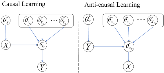
Figure 1: Data generating process under different causal models for both source and target domains, with domain identifiers $s$ and $t$ omitted for the distribution parameters.

Assumption 1 (Parametric IID data)

We assume the labeled source and unlabeled target samples are generated independently and identically under both causal learning and anti-causal learning. More precisely, the joint distribution of the data sequence pairs $P_{\theta^{*}_{s},\theta^{*}_{t}}({D_{t}^{U,n},D_{s}^{m}})$ can be written as

$$P_{\theta^{*}_{s},\theta^{*}_{t}}(D^{\textup{U},n}_{t},D_{s}^{m})=\prod_{i=1}^{n}P_{\theta_{t}^{*}}(X_{t}^{(i)})\prod_{j=1}^{m}P_{\theta_{s}^{*}}(X_{s}^{(j)},Y_{s}^{(j)}),$$

where $P_{\theta_{t}^{*}}(X_{t}^{(i)})$ is the marginal of $P_{\theta_{t}^{*}}(X_{t}^{(i)},Y_{t}^{(i)})$. We also assume $\theta^{*}_{t}$ and $\theta^{*}_{s}$ are points in the interior of $\Lambda$. Furthermore, in both models, the parametric families for the cause and potential outcomes are assumed to be known in advance.

Based on the models defined above, the excess risk in Equation (1) can be written as

$$\mathcal{R}(b) :=\mathbb{E}_{P_{\theta^{*}_{s}}(D^{m}_{s})P_{\theta^{*}_{t}}(D^{\textup{U},n}_{t},X^{\prime}_{t},Y^{\prime}_{t})}\left[\ell\left(b,Y^{\prime}_{t}\right)-\ell(b^{*},Y^{\prime}_{t})\right]$$

$$=\mathbb{E}_{\theta_{s},\theta_{t}}\left[\ell\left(b,Y^{\prime}_{t}\right)-\ell(b^{*},Y^{\prime}_{t})\right]$$ (18)

For simplicity, we use the notation $\mathbb{E}_{\theta_{s},\theta_{t}}[\cdot]$ (similarly, $\mathbb{E}_{\theta_{t}}[\cdot]$ and $\mathbb{E}_{\theta_{s}}[\cdot]$) to denote the expectation taken over all source and target samples drawn from ${P}_{\theta_{s}}$ and ${P}_{\theta_{t}}$.

4 Main Results

In this section, we will examine the excess risk for causal and anti-causal learning under various conditions of distribution shift, e.g., co-variate shift (Gretton et al., , 2009), target shift (Zhang et al., , 2013), concept drift (Cai and Wei, , 2021), etc. Before diving into the details, we informally outline our main results in Table 1 under log-loss. Recall that in both causal and anti-causal learning, the goal is to learn the conditional distribution $P_{T}(Y|X)$ such that the label $Y$ can be predicted from the feature $X$ in the target domain. In causal learning, this corresponds to learning the potential outcome random variables $Y_{t,x_{i}}$. However, the unlabeled target data $X_{t}$ (“cause” in this case) do not contain information about $Y_{t,x_{i}}$ as they are independent under the ignorability condition. Therefore, the unlabeled target data are not useful in the causal learning case, as indicated in the table. The usefulness of the source data depends on the models. When the labeling distribution is invariant across two domains (e.g., $P_{S}(Y|X)=P_{T}(Y|X)$), the source data help reduce excess risk by providing information about $Y_{t,x_{i}}$, which is identical to $Y_{s,x_{i}}$. The learning rate is then shown to be $O(\frac{k}{m})$, where $k$ is the number of parameters and $m$ is the size of the source sample. On the other hand, if $P_{S}(Y|X)\neq P_{T}(Y|X)$, the source data generally do not provide information about $Y_{t,x_{i}}$ and the excess risk does not converge to zero even with sufficient source and target data.

Causal Model	Conditions	Unlabeled Target	Source Data	Rate
$X\rightarrow Y$	$P_{S}(X)\neq P_{T}(X)$, $P_{S}(Y|X)\neq P_{T}(Y|X)$	✗	✗	-
	$P_{S}(X)\neq P_{T}(X)$, $P_{S}(Y|X)=P_{T}(Y|X)$	✗	✓	$O(\frac{k}{m})$
	$P_{S}(X)=P_{T}(X)$, $P_{S}(Y|X)\neq P_{T}(Y|X)$	✗	✗	-
	$P_{S}(X)=P_{T}(X)$, $P_{S}(Y|X)=P_{T}(Y|X)$	✗	✓	$O(\frac{k}{m})$
$Y\rightarrow X$	$P_{S}(Y)\neq P_{T}(Y)$, $P_{S}(X|Y)\neq P_{T}(X|Y)$	✓	✗	$O(\frac{1+k^{\prime}}{n})$
	$P_{S}(Y)\neq P_{T}(Y)$, $P_{S}(X|Y)=P_{T}(X|Y)$	✓	✓	$O(\frac{1}{n}+\frac{k^{\prime}}{n+m})$
	$P_{S}(Y)=P_{T}(Y)$, $P_{S}(X|Y)\neq P_{T}(X|Y)$	✓	✓	$O(\frac{k^{\prime}}{n}+\frac{1}{n+m})$
	$P_{S}(Y)=P_{T}(Y)$, $P_{S}(X|Y)=P_{T}(X|Y)$	✓	✓	$O(\frac{k^{\prime}+1}{m+n})$

Table 1: (Informal) results on effectiveness of source and unlabeled target data under causal and anti-causal learning problems.“✓” and “✗” marks indicate whether the data are useful or not for the prediction under the specific conditions and causal models. The rate illustrates the convergence for the excess risk under log-loss in terms of the target sample size $n$ and source sample size $m$. The “-” sign in the rate column means the risk will not converge to zero even if we have sufficient source and target data.

In anti-causal learning scenario ($Y\rightarrow X$, $P_{S}(X,Y)\neq P_{T}(X,Y)$), however, learning $P_{T}(Y|X)$ requires to estimate all the parameters of $Y_{t}$ and $X_{t,y_{i}}$. Unlike causal learning, where $P_{T}(Y|X)$ is fully represented by the potential outcome variables $Y_{t,x_{i}}$, in this case we need to infer $P_{T}(Y|X)$ from the joint distribution $P_{T}(X,Y)$. We will show that the unlabeled target data is always useful in anti-causal learning under certain conditions. The source data can also contribute to learning, depending on the assumptions we have made about the distribution shift. For example, if $P_{S}(Y)\neq P_{T}(Y)$ and $P_{S}(X|Y)\neq P_{T}(X|Y)$ with the independence assumption, there is no reason for the source data to be useful for prediction in the target domain. Therefore, the rate in this case is $O(\frac{k^{\prime}+1}{n})$, which solely depends on the number of unlabeled target data. Intuitively, this is the cost of learning $k^{\prime}+1$ parameters with $n$ unlabeled target samples. Under the target shift condition ($P_{S}(Y)\neq P_{T}(Y)$ and $P_{S}(X|Y)=P_{T}(X|Y)$), the source data helps in learning the potential outcome variables $X_{y_{i}},i=1,\ldots,k^{\prime}$, which is evinced in the rate $O(\frac{1}{n}+\frac{k^{\prime}}{m+n})$ that constitutes the learning of $Y_{t}$ (with associated parameter $\theta^{t*}_{Y}$) with a rate $O(\frac{1}{n})$ and $X_{t,y_{i}},i=1,\ldots,k^{\prime}$ (with associated parameters $\theta^{t*}_{X_{y_{i}}}$) with a rate $O(\frac{k^{\prime}}{n+m})$. Similarly, for the conditional shift ($P_{S}(Y)=P_{T}(Y)$ and $P_{S}(X|Y)\neq P_{T}(X|Y)$), the rate becomes $O(\frac{k^{\prime}}{n}+\frac{1}{m+n})$ where sufficient source data boosts the learning of $Y_{t}$ (associated with parameter $\theta^{t*}_{Y}$) with a rate $O(\frac{1}{m+n})$, but are not helpful for learning potential outcomes variables $X_{t,y_{i}}$.

As a special case of domain adaptation, we also consider SSL where $P_{S}(X,Y)=P_{T}(X,Y)$. Using the same arguments in causal and anti-causal models, we obtain a better rate of $O(\frac{k^{\prime}+1}{m+n})$ in anti-causal learning, where the unlabeled target data take effect on prediction, compared to $O(\frac{k}{m})$ in causal learning, where the unlabeled target data are not helpful. For readers interested in empirical verification of our results, we substantiate the analysis with a toy example, which can be found in Appendix A.

More generally, our analysis also holds for the case when the cause is discrete and the effect can be either discrete or continuous. This is practically useful since the datasets in many real classification problems are usually anti-causal with a finite label space $\mathcal{Y}$ (Schölkopf et al., , 2012; Zhang et al., , 2013; Gong et al., , 2016). Moreover, the assumption of parametric distribution can be weakened, i.e., the true distribution does not necessarily lie in the hypothesis space and may not be parametrized, which is usually known as the misspecified setting. In this case, our results can be easily extended under such a situation with the same intuitions (Li, , 1999; Van der Vaart, , 2000; Mourtada and Gaïffas, , 2019).

4.1 Connections with Other Bounds

Many theoretical results on generalization in domain adaptation depend on distributional conditions and algorithms. For example, based on the co-variate shift condition, Kpotufe and Martinet, (2018) propose the “transfer component” that evaluates the support overlap between the source and target domains, and derive the minimax rate for the generalization error. But such a notion cannot be generally applied to other distribution shift conditions. Similarly, Cai and Wei, (2021) determine the optimal minimax rate of convergence with the weighted kNN classifier using the notion of “relative signal exponent” based on the concept drift condition. Under the target shift condition, Maity et al., (2020) and Gong et al., (2016) derive the learning guarantees for the distribution reweighting strategies, which are algorithm dependent.

In contrast, our analysis is applicable to general distribution shift conditions, allowing a unified framework to analyze the learning performance from the causal perspective and providing a natural interpretation of the values of source and target data. Specifically, our result of the co-variate shift condition can be considered as a special case when $P_{T}(X)$ is absolutely continuous w.r.t. $P_{S}(X)$ in Kpotufe and Martinet, (2018), where the labeled source has the same value as the labeled target. The target shift result agrees with Maity et al., (2020) in the sense that the unlabeled target is equally useful as the labeled target data, achieving a rate of $O(\frac{1}{n})$. Under the concept drift condition, we argue that the excess risk does not converge, which is consistent with Theorem 3.1 in Cai and Wei, (2021) for a large relative signal exponent and no labeled target data. Moreover, we prove in Lemma 1 that the excess risk is minimax optimal under log-loss.

4.2 Information-theoretic Characterization

We will prove our main results in the subsequent section. For simplicity, we first consider the log-loss (also known as logarithmic loss), which is formally defined as follows.

Definition 2 (Log-loss)

Let the predictor $b$ be a probability distribution over the target label $Y^{\prime}_{t}$. The log-loss is then defined as,

$$\ell(b,Y^{\prime}_{t})=-\log b(Y^{\prime}_{t}).$$ (19)

Given the testing feature $X^{\prime}_{t}$, training data $D^{m}_{s}$ and $D^{U,n}_{t}$, we may view the predictor $b$ as the conditional distribution $Q(Y^{\prime}_{t}|D^{\textup{U},n}_{t},D^{m}_{s},X^{\prime}_{t})$ over the unseen target label given the testing feature $X^{\prime}_{t}$ and the training data $D^{m}_{s},D^{\textup{U},n}_{t}$. It could be proved that the true predictor $b^{*}$ is given by the underlying target distribution as $b^{*}(Y^{\prime}_{t})=P_{\theta^{*}_{t}}(Y^{\prime}_{t}|X^{\prime}_{t})$. Then the excess risk can be expressed as,

$$\mathcal{R}(b) =\mathbb{E}_{\theta^{*}_{t},\theta^{*}_{s}}\left[\log\frac{P_{\theta^{*}_{t}}(Y^{\prime}_{t}|X^{\prime}_{t})}{Q(Y^{\prime}_{t}|D^{\textup{U},n}_{t},D^{m}_{s},X^{\prime}_{t})}\right]$$ (20)

Concerning the choice of the predictor $Q(Y^{\prime}_{t}|D^{\textup{U},n}_{t},D^{m}_{s},X^{\prime}_{t})$, we first define $\Theta_{s}$ and $\Theta_{t}$ as random vectors over $\Lambda$, which can be interpreted as a random guess of $\theta^{*}_{s}$ and $\theta^{*}_{t}$. Note that $\Theta_{s}$ and $\Theta_{t}$ may share some common parameters, e.g., $\Theta_{s,i}=\Theta_{t,i}$ for $i$th entry. Then by mixture strategy (Merhav and Feder, , 1998; Xie and Barron, , 2000) we assign a probability distribution $\omega$ over $\Theta_{s}$ and $\Theta_{t}$ w.r.t. the Lebesgue measure to represent our prior knowledge and update the posterior with the incoming data to approximate the underlying distributions. That is,

$$Q(Y^{\prime}_{t}|D^{\textup{U},n}_{t},D^{m}_{s},X^{\prime}_{t})$$

$$=\frac{\int P_{\theta_{t}}(D^{\textup{U},n}_{t},X^{\prime}_{t},Y^{\prime}_{t})P_{\theta_{s}}(D^{m}_{s})\omega(\theta_{t},\theta_{s})d\theta_{t}d\theta_{s}}{\int P_{\theta_{t}}(X^{\prime}_{t})P_{\theta_{t}}(D^{\textup{U},n}_{t})P_{\theta_{s}}(D^{m}_{s})\omega(\theta_{t},\theta_{s})d\theta_{t}d\theta_{s}}$$

$$=\int P_{\theta_{t}}(Y^{\prime}_{t}|X^{\prime}_{t})P(\theta_{t},\theta_{s}|X^{\prime}_{t},D^{m}_{s},D^{\textup{U},n}_{s})d\theta_{s}d\theta_{t}.$$ (21)

We can interpret (21) as estimating $Y^{\prime}$ in a two-step procedure. With a prior distribution $\omega$, the first step is to learn the parameters $\theta_{s}$, $\theta_{t}$ with the joint posterior $P(\theta_{s},\theta_{t}|D^{m}_{s},D^{\textup{U},n}_{t},X^{\prime}_{t})$. In the second step, the learned $\theta_{t}$ is applied for prediction in terms of the parametric distribution $P_{\theta_{t}}(Y^{\prime}_{t}|X^{\prime}_{t})$. One way to comprehend the mixture strategy is that we encode our prior knowledge over target and source domain distributions in terms of the prior distribution $\omega(\Theta_{s},\Theta_{t})$, and different distribution shift conditions correspond to different priors. By the mixture strategy, we give the excess risk under log-loss.

Theorem 1 (Excess Risk with Log-loss)

Under log-loss, let the predictor $Q$ be the distribution in (21) with the prior distribution $\omega(\Theta_{s},\Theta_{t})$. Then the excess risk can be expressed as

$$\mathcal{R}(b)=I(Y^{\prime}_{t};\theta^{*}_{t},\theta^{*}_{s}|D^{m}_{s},D^{\textup{U},n}_{t},X^{\prime}_{t}),$$ (22)

where $I(Y^{\prime}_{t};\theta^{*}_{t},\theta^{*}_{s}|D^{m}_{s},D^{\textup{U},n}_{t},X^{\prime}_{t})$ denotes the conditional mutual information (CMI) $I(Y^{\prime}_{t};\Theta_{t},\Theta_{s}|D^{m}_{s},D^{\textup{U},n}_{t},X^{\prime}_{t})$ evaluated at $\Theta_{t}=\theta^{*}_{t}$ and $\Theta_{s}=\theta^{*}_{s}$.

All proofs in this paper can be found in Appendix. A similar learning strategy can be used for more general loss functions. Given a general loss function $\ell$, we define the predictor $b$ as

$$b={\text{argmin}}_{b}\mathbb{E}_{Q}\left[\ell(b,Y^{\prime}_{t})|X^{\prime}_{t},D^{U,n}_{t},D^{m}_{s}\right],$$ (23)

with the choice of the mixture strategy

$$Q(X^{\prime}_{t},Y^{\prime}_{t},D^{n}_{t},D^{m}_{s})=\int P_{\theta_{t},\theta_{s}}(X^{\prime}_{t},Y^{\prime}_{t},D^{U,n}_{t},D^{m}_{s})\omega(\theta_{t},\theta_{s})d\theta_{t}d\theta_{s}$$

for some prior $\omega$. The optimal predictor is then given by

$$b^{*}={\text{argmin}}_{b}\mathbb{E}_{\theta^{*}_{t}}\left[\ell(b,Y^{\prime}_{t})|D^{U,n}_{t},X^{\prime}_{t}.\right]$$ (24)

We have the following theorem for $\beta$-exponential concave loss functions as follows.

Theorem 2 (Excess Risk with Exponential Concave Loss)

Assume the loss function is $\beta$-exponentially concave of $b$ for any $y$. Then the excess risk induced by $b$ and $b^{*}$ in Equation (23) and (24) can be bounded as

$$\mathcal{R}(b)\leq\frac{1}{\beta}I(Y^{\prime}_{t};\theta^{*}_{t},\theta^{*}_{s}|D^{m}_{s},D^{\textup{U},n}_{t},X^{\prime}_{t}).$$ (25)

The log-loss can be regarded as a special case with $\beta=1$. One can refer to Lemma 1 (also the proof) in Zhu, (2020) for more details and comments, which we will not repeat in our context. Likewise, if the loss function is bounded, we arrive at the following theorem.

Theorem 3 (Excess Risk with Bounded Loss)

Assume the loss function satisfies $|\ell(b,y)-\ell(b^{*},y)|\leq M$ for any observation $y$ and any two predictors $b,b^{*}$. Then the excess risk can be bounded as

$$\mathcal{R}(b)\leq M\sqrt{2I(Y^{\prime}_{t};\theta^{*}_{t},\theta^{*}_{s}|D^{m}_{s},D^{\textup{U},n}_{t},X^{\prime}_{t})}.$$ (26)

From the above theorems, we can see the analogy that the expected regrets induced by the mixture strategy are both characterized by CMI evaluated at $\theta^{*}_{t}$ and $\theta^{*}_{s}$. Note that these results are applicable to both causal and anti-causal learning problems. Nevertheless, the characterization of learning performance in its present form is less informative because it does not show the effect of sample sizes and causal directions. To this end, we make some regularity assumptions on the parametric conditions (Clarke and Barron, , 1990; Merhav and Feder, , 1998; Zhu, , 2020) and define the proper prior to obtain an asymptotic approximation.

Assumption 2 (Parametric Distribution Conditions)

With the aforementioned parameterisation, let $\mathbf{\theta}^{*}=(\theta^{*}_{s},\theta^{*}_{t})$ denote the underlying parameters for labeled source and unlabeled target data. We assume:

• Condition 1: The source and target distributions $P_{\theta_{s}}(X_{s},Y_{s})$ and $P_{\theta_{t}}(X_{t})$ is twice continuously differentiable at $\theta_{s}^{*}$ and $\theta^{*}_{t}$ for almost every $(X_{s},Y_{s})$ and $X_{t}$.

• Condition 2: Define the Fisher information matrix

  $$I_{s} =-\mathbb{E}_{\theta^{*}_{s}}[\nabla^{2}\log P(X_{s},Y_{s}|\theta^{*}_{s})],$$

  $$I_{t} =-\mathbb{E}_{\theta^{*}_{t}}[\nabla^{2}\log P(X_{t}|\theta^{*}_{t})],$$

  $$I_{0} =-\mathbb{E}_{\theta^{*}}[\nabla^{2}\log P(X_{t},X_{s},Y_{s}|\theta^{*})].$$

  We assume $I_{s}$ and $I_{t}$ are positive definite and it holds that $I_{0}$ is also positive definite.

• Condition 3 (Clarke and Barron, , 1990): we assume that the convergence of a sequence of parameter values is equivalent to the weak convergence of the distributions they index. Particularly:

  $$\theta_{s}\rightarrow\theta^{*}_{s} \Leftrightarrow P_{\theta_{s}}(X,Y)\rightarrow P_{\theta^{*}_{s}}(X,Y),$$

  $$\theta_{t}\rightarrow\theta^{*}_{t} \Leftrightarrow P_{\theta_{t}}(X)\rightarrow P_{\theta_{t}^{*}}(X),$$

  for source and target domains, respectively.

Due to the space limit, we only include these three key conditions for the parametric distributions under both causal and anti-causal learning models, and other technical conditions can be found in Appendix B.1.

Assumption 3 (Proper Prior)

We assume that the prior distribution $\omega(\Theta_{s},\Theta_{t})$ is continuous and positive over its whole support.

We impose these conditions on parametric distributions with the proper prior to ensure that the posterior distribution of $\Theta_{t}$ and $\Theta_{s}$ asymptotically concentrates on neighbourhoods of $\theta^{*}_{t}$ and $\theta^{*}_{s}$ under both causal models given sufficient source and target data. In particular, the positive definite Fisher information matrix and parameter uniqueness assumption imply that $\theta^{*}_{t}$ and $\theta^{*}_{s}$ are identifiable within $\Lambda$. We also impose some technical conditions to ensure that the posterior of the parameters converges to their true values at an appropriate rate.

4.3 Excess Risk in Causal Learning

In this section, we will characterize the excess risk asymptotically under the causal learning. We firstly consider the learning scenario when $P_{S}(Y|X)=P_{T}(Y|X)$, which corresponds to SSL if $P_{T}(X)=P_{S}(X)$ and covariate shift regime otherwise. The random vector $\Theta_{s}$ and $\Theta_{t}$ can be explicitly written as

$$\Theta_{s}=(\Theta^{s}_{X},\Theta^{s}_{Y_{x_{1}}},\cdots,\Theta^{s}_{Y_{x_{k}}})=(\Theta^{s}_{X},\Theta^{s}_{Y_{X}}),$$ (27)

$$\Theta_{t}=(\Theta^{t}_{X},\Theta^{t}_{Y_{x_{1}}},\cdots,\Theta^{t}_{Y_{x_{k}}})=(\Theta^{t}_{X},\Theta^{t}_{Y_{X}}),$$ (28)

where $\Theta_{Y_{X}}=(\Theta_{Y_{x_{1}}},\cdots,\Theta_{Y_{x_{k}}})$ for succinctness. We assume $\Theta^{t}_{X}$ and $\Theta^{s}_{X}$ are independent of $\Theta^{s}_{Y_{X}}$ and $\Theta^{t}_{Y_{X}}$, but we will keep $\Theta^{s}_{Y_{X}}$ and $\Theta^{t}_{Y_{X}}$ identical according to the assumption $P_{S}(Y|X)=P_{T}(Y|X)$, written as $\Theta^{st}_{Y_{X}}$. With the proper prior distribution, we simplify the mixture distribution $Q$ as follows by omitting the unlabeled target data due to the ignorability condition:

$$Q(Y^{\prime}_{t}|D^{\textup{U},n}_{t},D^{m}_{s},X^{\prime}_{t})=\int P(Y^{\prime}_{t}|\theta^{st}_{Y_{X}},X^{\prime}_{t})P(\theta^{st}_{Y_{X}}|D^{m}_{s})d\theta^{st}_{Y_{X}},$$

where the knowledge transfer depends on the conditional posterior $P(\theta^{st}_{Y_{X}}|D^{m}_{s})$. Since $P_{S}(Y|X)=P_{T}(Y|X)$, without any labels from the target domain, we can only learn the parameters of the potential outcomes from the source data. On the other hand, if the assumption $P_{S}(Y|X)=P_{T}(Y|X)$ does not hold, namely, the concept drift if $P_{S}(X)=P_{T}(X)$ and general shift condition otherwise, the mixture strategy in (21) becomes

$$Q(Y^{\prime}_{t}|D^{\textup{U},n}_{t},D^{m}_{s},X^{\prime}_{t}) =\int P_{\theta^{t}_{Y_{X^{\prime}_{t}}}}(Y^{\prime}_{t})\omega(\theta^{t}_{Y_{X^{\prime}_{t}}})d\theta^{t}_{Y_{X^{\prime}_{t}}}$$

due to the mutually independence properties on the distribution parameters. In this case, neither the unlabeled target data nor the source data are useful for the estimation, the prediction is only piloted by the prior distribution $\omega(\theta^{t}_{Y_{X}})$ as the initial estimate for $\theta^{t*}_{Y_{X}}$. As a result, the excess risk in this case does not go to zero even if we have enough source and target data. To formally state the idea, we give the asymptotic estimation in the following main theorem.

Theorem 4 (Excess Risk with Causal Learning)

In addition to Assumption 1,2 and 3, we also assume that $X$ causes $Y$ in both source and target domains. Let $\Theta_{s}$ and $\Theta_{t}$ be parameterized in (27) and (28). As $m\rightarrow\infty$, the mixture strategy under log-loss yields:

• (General shift and Concept drift) For any $P_{\theta^{t*}_{X}}(X)\ll P_{\theta^{s*}_{X}}(X)$, if $P_{S}(Y|X)\neq P_{T}(Y|X)$:

  $$\mathcal{R}(b)=\mathbb{E}_{\theta^{t*}_{X}}[\textup{KL}(P_{\theta^{t*}_{Y_{X^{\prime}_{t}}}}(Y^{\prime}_{t})\|Q(Y^{\prime}_{t}|X^{\prime}_{t})],$$ (29)

  where $Q(Y^{\prime}_{t}|X^{\prime}_{t})=\int P_{\theta^{t}_{Y_{X^{\prime}_{t}}}}(Y^{\prime}_{t})\omega(\theta^{t}_{Y_{X^{\prime}_{t}}})d\theta^{t}_{Y_{X^{\prime}_{t}}}$ for a certain prior $\omega$ over $\Theta^{t}_{Y_{X^{\prime}_{t}}}$.

• (Co-variate shift and SSL) For any $P_{\theta^{t*}_{X}}(X)\ll P_{\theta^{s*}_{X}}(X)$, if $P_{S}(Y|X)=P_{T}(Y|X)$:

  $$\mathcal{R}(b)\asymp\frac{k}{m}.$$ (30)

From the above theorem, it is clear that the target data are not useful without labels and $n$ does not occur in the rate. This is understandable because such data do not contain information about $P(Y|X)$ due to the independence assumptions between $X$ and $Y_{x_{i}}$. If the conditional distribution remains unchanged between source and target domains, the excess risk converges with the rate of $O(\frac{k}{m})$.

4.4 Excess Risk in Anti-Causal Learning

We now turn to the opposite causal direction where $Y\rightarrow X$. Similarly, we define the random variable $\Theta_{s}$ and $\Theta_{t}$ with the same form as  (27) and (28) by

$$\Theta_{s}=(\Theta^{s}_{Y},\Theta^{s}_{X_{y_{1}}},\cdots,\Theta^{s}_{X_{y_{k^{\prime}}}})=(\Theta^{s}_{Y},\Theta^{s}_{X_{Y}}),$$ (31)

$$\Theta_{t}=(\Theta^{t}_{Y},\Theta^{t}_{X_{y_{1}}},\cdots,\Theta^{t}_{X_{y_{k^{\prime}}}})=(\Theta^{t}_{Y},\Theta^{t}_{X_{Y}}).$$ (32)

At this stage, we do not particularize any conditions on the parameters. From the Bayes rule, we rewrite the mixture distribution $Q$ in terms of the above parameterization as

$$Q(Y^{\prime}_{t}|D^{\textup{U},n}_{t},D^{m}_{s},X^{\prime}_{t}) =\frac{\int P_{\theta_{t}}(D^{\textup{U},n}_{t},X^{\prime}_{t},Y^{\prime}_{t})P_{\theta_{s}}(D^{m}_{s})\omega(\theta_{t},\theta_{s})d\theta_{t}d\theta_{s}}{\int P_{\theta_{t}}(X^{\prime}_{t})P_{\theta_{t}}(D^{\textup{U},n}_{t})P_{\theta_{s}}(D^{m}_{s})\omega(\theta_{t},\theta_{s})d\theta_{t}d\theta_{s}}$$

$$=\frac{\int P(Y^{\prime}_{t}|\theta_{t},X^{\prime}_{t})P(\theta_{t}|D^{\textup{U},n}_{t},X^{\prime}_{t},\theta_{s})d\theta_{t}P(\theta_{s}|D^{m}_{s})d\theta_{s}}{\int P(\theta_{t}|D^{\textup{U},n}_{t},X^{\prime}_{t},\theta_{s})d\theta_{t}P(\theta_{s}|D^{m}_{s})d\theta_{s}}$$

$$=\int P(Y^{\prime}_{t}|\theta_{t},X^{\prime}_{t})P(\theta_{t}|D^{\textup{U},n}_{t},X^{\prime}_{t},\theta_{s})d\theta_{t}P(\theta_{s}|D^{m}_{s})d\theta_{s}.$$

To interpret, the mixture strategy first provides an estimate of $\theta_{s}$ from the source data, then knowledge is transferred from $\theta_{s}$ to $\theta_{t}$ with the prior distribution $\omega(\theta_{t}|\theta_{s})$, which induces the posterior $P(\theta_{t}|X^{\prime}_{t},D^{U,n}_{t},\theta_{s})$ along with the features $X^{\prime}_{t},D^{U,n}_{t}$ in the target domain, since the unlabeled data may contain all the information of $\theta^{*}_{t}$ under the anti-causal parameterisation. Eventually, the prediction of $Y^{\prime}_{t}$ will be based on the estimated $\theta_{t}$ and $X^{\prime}_{t}$.

With condition 3 under Assumption 2, we require that the true parameters $\theta^{*}_{t}$ are identifiable given sufficient unlabeled target data, where its distribution is a mixture distribution, i.e., $\sum_{y\in\mathcal{Y}}P_{\theta_{Y}}(y)P_{\theta_{X_{y}}}(X)$. In general, this is a strong condition where the mixture distributions, such as the Bernoulli mixture, do not satisfy the assumption (Gyllenberg et al., , 1994) and the parameters within their support are not identifiable. But for certain types of families, the parameters are identifiable up to label swapping, such as Gaussian (Teicher, , 1963), exponential families (Barndorff-Nielsen, , 1965), and many other finite continuous mixture distributions (McLachlan et al., , 2019). Under label swapping, the posterior of the parameters approaches one of all permutations (Marin et al., , 2005) and our result holds only up to the permutation. To solve such a problem, the methods proposed include the specification of parameterization constraints (Marin et al., , 2005; McLachlan et al., , 2019), a relabeling algorithm (Stephens, , 2000), and constraint clustering (Grün and Leisch, , 2009). Once the label swapping is addressed, most mixed distributions are identifiable (Titterington et al., , 1985; McLachlan et al., , 2019) and our results hold as well. For illustration, we give a simple example of a categorical mixture distribution identifiable by adding structural constraints to the parameterization in Appendix A. We will now consider different distribution shift scenarios under anti-causal learning and derive the corresponding asymptotic estimation for the excess risk.

Theorem 5 (Excess Risk with Anti-causal Learning)

In addition to Assumptions 1, 2 and 3, we also assume $Y\rightarrow X$ in both source and target domains. Let $\Theta_{s}$ and $\Theta_{t}$ be parameterised in (31) and (32). As $m\asymp n^{p}$ for some $p>0$ and $n\rightarrow\infty$, the mixture strategy under log-loss yields:

• (General shift) If $P_{S}(Y)\neq P_{T}(Y)$, $P_{S}(X|Y)\neq P_{T}(X|Y)$,

  $$\mathcal{R}(b)\asymp\frac{1+k^{\prime}}{n}.$$ (33)

• (Conditional shift) If $P_{S}(Y)=P_{T}(Y)$, $P_{S}(X|Y)\neq P_{T}(X|Y)$,

  $$\mathcal{R}(b)\asymp\frac{k^{\prime}}{n}+\frac{1}{n\vee n^{p}}.$$ (34)

• (Target shift) If $P_{S}(Y)\neq P_{T}(Y)$, $P_{S}(X|Y)=P_{T}(X|Y)$,

  $$\mathcal{R}(b)\asymp\frac{1}{n}+\frac{k^{\prime}}{n\vee n^{p}}.$$ (35)

• (SSL) If $P_{S}(Y)=P_{T}(Y)$, $P_{S}(X|Y)=P_{T}(X|Y)$,

  $$\mathcal{R}(b)\asymp\frac{k^{\prime}+1}{n\vee n^{p}}.$$ (36)

In contrast to causal learning, in the general shift case we can achieve good generalization ability only with the unlabeled target data, while the source data do not help at all. In the conditional shift and target shift cases, we can further show that the source data can only help improve the excess risk from $O(\frac{k^{\prime}+1}{n})$ to $O(\frac{k^{\prime}+1-j}{n}+\frac{j}{n\vee n^{p}})$ depending on how many $j$ common parameters $\theta^{*}_{s}$ and $\theta^{*}_{t}$ share. Intuitively, $O(\frac{k^{\prime}+1-j}{n})$ can be viewed as the learning cost for $k^{\prime}+1-j$ domain-specific parameters and $O(\frac{j}{n\vee n^{p}})$ as the learning cost for domain-sharing parameters. Therefore, the source data are incapable of changing the overall rate since the unlabeled target data always dominates the rate. In SSL, the rate $O(\frac{k^{\prime}+1}{n\vee n^{p}})$ indicates that unlabeled target data are as useful as the labeled source data and that sufficient source data (e.g., $p>1$) can indeed change the convergence rate. The results show that the learning complexity under different causal directions will vary. This crucial distinction discloses how the causal relationships affect the model complexity and its generalization ability.

Our results in Theorem 1, 4, 5 establish the convergence rate for the mixture strategy. Here we show that this strategy is in fact optimal for log-loss.

Lemma 1 (Worst-Case Excess Risk)

For log-loss,

$$\min_{b}\max_{\theta^{*}_{s},\theta^{*}_{t}}\mathcal{R}(b)=\max_{\omega(\theta_{s},\theta_{t})}I(Y^{\prime}_{t};\Theta_{t},\Theta_{s}|D^{m}_{s},D^{\textup{U},n}_{t},X^{\prime}_{t}),$$

where $(\Theta_{t},\Theta_{s})$ is endowed with some prior distribution $\omega$.

This lemma exactly characterizes the excess risk for log-loss in the worst case. It shows that the worst-case regret is captured by the same CMI term as in Theorem 1, although maximized w.r.t. the prior distribution over the source and target parameters. However, it can be shown that the maximization does not change the convergence rate of the mutual information term (Clarke and Barron, , 1994; Merhav and Feder, , 1998). In other words, the convergence rate in Theorem 4, 5 is indeed optimal and cannot be improved using a different learning algorithm. Even though we only consider the log-loss in previous analysis, the results can be extended straightforwardly in the case of other general loss functions, such as exponentially concave or bounded losses, where the excess risk is captured by the same CMI term in Theorem 1 (see Theorem 3 for bounded losses as an example).

5 Conclusions

This paper proposes a probabilistic framework that articulates the connection between transfer learning and causal mechanisms. We explicitly depict the rate of the learning performance under different causal mechanisms and domain shift conditions, from which the usefulness of the source and target data is manifested. However, in our analysis, the ignorability assumption (e.g., $X$ and $Y$ are unconfounded) is crucial. The possible future challenge could be performing a similar analysis for the case with more than two variables (e. g. causal models with con-founders), which improves the generality and applicability in real-world problems.

Appendix A Experiments

We will firstly numerically confirm our main results using a toy example. Then we elaborate on the case when the data can be modeled both as causal learning and anti-causal learning. We show that the model selection closely hinges on the ways of parametrization, the number of samples and the distribution shift conditions.

A.1 A toy example

We will numerically confirm our main results using a toy example. We consider a simple example where $\mathcal{Y}=\{0,1\}$ and $\mathcal{X}=\{1,2,3,4\}$. In the causal learning, we model the data distributions as

$$X\sim\textup{Cat}(\theta_{x_{1}},\theta_{x_{2}},\theta_{x_{3}},\theta_{x_{4}})$$

$$Y_{x_{i}}\sim\textup{Ber}(\theta_{Y_{x_{i}}})\textup{ for }i=1,2,3,4.$$

We set $\theta^{t*}_{X}=(0.25,0.25,0.25,0.25)$ and $\theta^{t*}_{Y_{X}}=(0.3,0.4,0.5,0.6)$ for synthetic experiments, and we will vary $\theta^{s*}_{X}=(0.6,0.1,0.1,0.2)$ and $\theta^{s*}_{Y_{X}}=(0.5,0.5,0.3,0.5)$ for the co-variate shift and concept drift conditions, respectively. The parameters are estimated using the maximum likelihood algorithm and used in the prediction. We run the experiments 3000 repeatedly and the results are shown in Figure 2. For general shift case in (a), we fix $m=2000$ and vary $n$ from 500 to 16000 and it can be seen that with the unlabeled target sample increasing, the risk will remain around $0.34$ and hence does not converge in this case. We sketch the regret for co-variate shift and semi-supervised learning in the figures (b) and (d), here we fix $n=2000$ and vary $m$ from 500 to 16000. It can be seen in that $\mathcal{R}(b)$ in blue converges to zero with $m$ increasing in these two cases, then we also plot the $\mathcal{R}(b)^{-1}$ in red to show the rate. The reciprocal of the excess risk is linear in the source sample size, which coincides with our theoretical analysis. It is worth pointing out that the slopes are different in these two cases because the quantity will depend on the Fisher information matrix of $P_{\theta^{s*}_{Y_{X}}}(Y)$ and the distribution of the co-variate $X$ varies across two domains. For concept drift learning in (c), we fix $n=2000$ and vary $m$ from 500 to 16000. Similar to general shift case, the excess risk is maintaining around 0.34 as well, which is independent of the source sample size $m$.

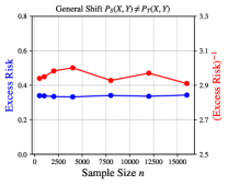
(a) Vary $n$

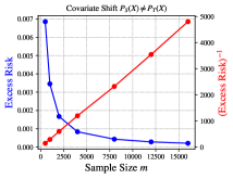
(b) Fix $n$, vary $m$

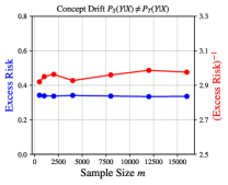
(c) Fix $n$, vary $m$

(d) Fix $n$, vary $m$

Figure 2: Excess risk comparisons under causal learning. (a) and (c) represents the results of $\mathcal{R}(b)$ for general shift case and concept drift learning, where we vary $n$ from 500 to 16000 in (a), and fix $n=2000$ but vary $m$ from 500 to 16000 in (c). We sketch the results $\mathcal{R}(b)$ for co-variate shift and semi-supervised learning in (b) and (d), here we fix $n=2000$ and vary $m$ from 500 to 16000. We also plot $\mathcal{R}(b)^{-1}$ to show the rate w.r.t. $m$. We plot all excess risks in blue and their reciprocals in red. All results are derived by 3000 experimental repeats.

In the anti-causal learning, we will model the distributions of the potential outcome random variables as

$$Y \sim\textup{Ber}(\theta_{Y}),$$

$$X_{0} \sim\textup{Cat}(\theta_{{0}},\theta_{{0}}+0.55,\theta_{{0}}+0.2,0.25-3\theta_{{0}}),$$

$$X_{1} \sim\textup{Cat}(\theta_{{1}},\theta_{{1}}+0.25,0.4-3\theta_{{1}},\theta_{{1}}+0.35).$$

For experiments, we set $\theta^{t*}_{Y}=0.5$ and $\theta^{t*}_{X_{0}}=\theta^{t*}_{X_{1}}=0.05$ as an example, and we will vary $\theta^{s*}_{Y}=0.7$ and $\theta^{s*}_{X_{0}}=\theta^{t*}_{X_{1}}=0.01$ for the target shift and conditional shift conditions, respectively. Using the maximum likelihood algorithm, we sketch the results in Figure 3. For the general shift case in (a), the excess risk converges as $n$ becomes larger, and more explicitly $\mathcal{R}(b)^{-1}$ is linear in $n$, which confirms our theoretical result. For target shift and conditional shift in (b) and (c), it can be seen in that $\mathcal{R}(b)$ converges to a non-zero value $\lambda$ with $m$ increasing in these two cases, then we also plot the $(\mathcal{R}(b)-\lambda)^{-1}$ to show the rate w.r.t. the sample size $m+n$. These two curves indicate that the source data can only help reduce the excess risk up to a constant. For semi-supervised learning in (d), as expected, the excess risk will converge to zero as $m$ increases. It is also observed that the slope of the reciprocal is higher compared to general shift condition, implying the source data contain more information than the unlabeled target data and lead to higher scaling factor $c$ (e.g., $O(\frac{c}{m})$) in the rate. We empirically depict the rate of the learning performance under different causal mechanisms and domain shift conditions, from which the usefulness of the source and target data is manifested.

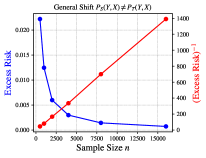
(a) Vary $n$

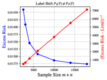
(b) Fix $n$, vary $m$

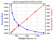
(c) Fix $n$, vary $m$

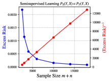
(d) Fix $n$, vary $m$

Figure 3: Excess risk comparisons under anti-causal learning. (a) represents the results of $\mathcal{R}(b)$ and $\mathcal{R}(b)^{-1}$ for general shift case, and we vary $n$ from 500 to 16000. We sketch the results $\mathcal{R}(b)$ for label shift, label concept drift and semi-supervised learning in (b), (c) and (d). Here we fix $n=2000$ and vary $m$ from 500 to 16000. It can be seen in that $\mathcal{R}(b)$ converges to a non-zero value $\lambda$ with $m$ increasing in (b) and (c), then we also plot $(\mathcal{R}(b)-\lambda)^{-1}$ to show the rate w.r.t. $m+n$. We plot all the excess risks in blue and their reciprocals in red. All results are derived by 3000 experimental repeats.

A.2 Model Selection from a causality perspective

Although in this work we primarily focus on the setup where the task is known to be either causal learning or anti-causal learning, it is also interesting to consider the scenario when the data can be modeled in both directions. If this is the case, our results imply that we should take advantage of this property and use whichever model that achieves a better learning performance. This can be viewed as a model selection problem. Referring to the Table 1, for semi-supervised learning, the rate from the causal direction will be $O(\frac{k}{m})$ while $O(\frac{k^{\prime}+1}{m+n})$ for anti-causal learning. If we have abundant source data ($n\ll m$) and $k<k^{\prime}+1$, fitting from the causal direction will be easier. In contrast, if we have abundant target data ($m\ll n$), then fitting from the anti-causal direction will be more favourable. Using similar arguments in the transfer learning scenarios, if the co-variate shift assumption does not hold, the source data will be unhelpful from the causal direction, and we should always fit from the anti-causal direction. Otherwise, the model selection is, again, determined by the sample sizes $m$ and $n$.

Overall, if a general transfer learning task can be modeled in both causal and anti-causal directions, both models can be more favourable than the other option depending on how we do the parameterisation, how many data samples we have and how different the source and target domains are.

Appendix B Proofs

B.1 Technical Conditions

We make following three additional technical conditions along with Assumption 2 for the parametric distributions under both causal and anti-causal learning.

• Condition 4: Assume that for all $\theta_{s}$ in some neighbourhood of $\theta^{*}_{s}$ and $\theta_{t}$ in some neighbourhood of $\theta^{*}_{t}$, the normalized Rényi divergences of order $1+\lambda$, the following holds

  $$\log\int P_{\theta^{*}_{s}}(x,y)^{1+\lambda}P_{\theta_{s}}(x,y)^{-\lambda}dxdy<\infty,$$ (37)

  $$\log\int P_{\theta^{*}_{t}}(x)^{1+\lambda}P_{\theta_{t}}(x)^{-\lambda}dx<\infty$$ (38)

  for sufficiently small $\lambda>0$.

• Condition 5: Assume that for all $\theta_{s}$ in some neighbourhood of $\theta^{*}_{s}$ and $\theta_{t}$ in some neighbourhood of $\theta^{*}_{t}$, the moment generating function is bounded as

  $$\mathbb{E}_{\theta^{*}_{s}}\left[e^{\lambda\frac{\partial^{2}}{\partial\theta_{j}\partial\theta_{k}}\log p(X_{s},Y_{s}\mid\theta_{s})}\right]<\infty,$$ (39)

  $$\mathbb{E}_{\theta^{*}_{t}}\left[e^{\lambda\frac{\partial^{2}}{\partial\theta_{j}\partial\theta_{k}}\log p(X_{t}\mid\theta_{t})}\right]<\infty,$$ (40)

  for all $j,k=1,\ldots,d$ with some small $\lambda>0$, where $d$ is determined based on the causal models and conditional shifting conditions.

• Condition 6: Let $l_{s}:=\left[(\nabla\log p\left(X,Y\mid\theta^{*}_{s}\right)),\mathbf{0}_{d^{\prime\prime}}\right]^{T}$, $l_{t}:=[\mathbf{0}_{d^{\prime\prime}},\nabla\log p\left(X\mid\theta^{*}_{t}\right)]^{T}$, where $\mathbf{0}_{d^{\prime\prime}}$ denotes the zero vector with length $d^{\prime\prime}$, and $d^{\prime\prime}$ denotes the number of domain-specific parameters which will be specified later. We also define $l^{\prime}_{s},l^{\prime}_{t}$ as an independent copy of $l_{s}$ and $l_{t}$, respectively. We assume the moment generating functions

  $$\mathbb{E}\left[e^{\lambda l_{s}^{T}I_{0}l_{s}}\right],\mathbb{E}\left[e^{\lambda l_{s}^{T}I_{0}l^{\prime}_{s}}\right],\mathbb{E}\left[e^{\lambda l_{t}^{T}I_{0}l_{t}}\right],$$

  $$\mathbb{E}\left[e^{\lambda l^{T}_{t}I_{0}l^{\prime}_{t}}\right],\mathbb{E}\left[e^{\lambda l^{T}_{t}I_{0}l_{s}}\right]$$

  exist for some small enough $\lambda>0$.

Remark 1

These three technical conditions are adopted and modified from Zhu, (2020) to ensure that the posterior of the parameters converges to their true values at an appropriate rate for both source and target domains. We will mainly use these conditions for asymptotic estimation of KL divergence, e.g., see proof of Lemma 2.

B.2 Mixture Asymptotics Lemma

Lemma 2 (Mixture Asymptotics)

Under Assumption 1,2,3 and assume $m\asymp n^{p}$ for some $p>0$ and let $n\rightarrow\infty$, then the mixture strategy yields

$$D(P_{\theta^{*}}(D^{m}_{s},D^{U,n}_{t})\|Q(D^{m}_{s},D^{U,n}_{t}))=\frac{d}{2}\log\frac{1}{2\pi e}+\log\frac{1}{\omega(\theta^{*})}+\frac{1}{2}\log\operatorname{det}(I_{st})+o(\frac{1}{n\vee m}),$$ (41)

where $\theta^{*}\in\mathbb{R}^{d}$ denotes the total parameters that characterize the source and target distributions and $d$ denotes the total dimension, depending on the causal directions and distribution shifting conditions. The Fisher information matrix associated with $D^{m}_{s}$ and $D^{U,n}_{t}$ is defined as $I_{st}=-\mathbb{E}_{\theta^{*}}[\nabla^{2}\log P(D^{m}_{s},D^{U,n}_{t}|\theta^{*})]$.

Proof 

The proof and result is a generalization of Clarke and Barron, (1990); Zhu, (2020) with some modifications to fit our purpose. Without the loss of generality, we first assume that the source parameter and target parameter will have $\tilde{k}+1-c$ domain-specific parameters and $c$ domain-sharing parameters, where $\tilde{k}=k$ for causal learning and $\tilde{k}=k^{\prime}$ for anti-causal learning. $c$ will vary under different shift conditions. For example, under the target shift condition in anti-causal learning, $c$ will be $k^{\prime}$ for identical parameters $\theta_{X_{y_{i}}}$ in both domains; In conditional shift condition, $c=1$ since $\theta^{s*}_{Y}=\theta^{t*}_{Y}$. With a little abuse of notation in this section, we denote the true source specific parameters by $\theta^{*}_{s}\in\mathbb{R}^{\tilde{k}+1-c}$, the target specific parameters by $\theta^{*}_{t}\in\mathbb{R}^{\tilde{k}+1-c}$ and the domain-sharing parameters as $\theta^{*}_{c}\in\mathbb{R}^{c}$. Then the source data $(X,Y)$ is drawn from the distribution $P_{\theta^{*}_{c},\theta^{*}_{s}}$ and the target data $X$ is drawn from the distribution $P_{\theta^{*}_{c},\theta^{*}_{t}}$ under such parameterization. For simplicity, we can write the joint domain parameters $\mathbf{\theta^{*}}=(\theta^{*}_{c},\theta^{*}_{s},\theta^{*}_{t})$ and the joint distribution for the source domain data and target domain data is expressed by

$$P_{\mathbf{\theta^{*}}}(D^{m}_{s},D^{U,n}_{t})=P_{\theta^{*}_{c},\theta^{*}_{s}}(D^{m}_{s})P_{\theta^{*}_{c},\theta^{*}_{t}}(D^{U,n}_{t})=\prod_{i=1}^{m}P_{\theta^{*}_{c},\theta^{*}_{s}}(D^{m}_{s})\prod_{j=1}^{n}P_{\theta^{*}_{c},\theta^{*}_{t}}(D^{U,n}_{t}).$$ (42)

Based on the notations above, we define the score functions by

$$l_{s}(\theta_{s},\theta_{c}) =\nabla\log P(D^{m}_{s}|\theta_{s},\theta_{c}),$$ (43)

$$l_{t}(\theta_{t},\theta_{c}) =\nabla\log P(D^{U,n}_{t}|\theta_{t},\theta_{c}),$$ (44)

$$l_{st}(\theta) =\nabla\log P(D^{U,n}_{t},D^{m}_{s}|\theta).$$ (45)

Note that

$$l_{st}(\theta^{*})=\begin{bmatrix}l_{s}(\theta^{*}_{s},\theta^{*}_{c})\\ \mathbf{0}_{\tilde{k}+1-c}\end{bmatrix}+\begin{bmatrix}\mathbf{0}_{\tilde{k}+1-c}\\ l_{t}(\theta^{*}_{t},\theta^{*}_{c})\end{bmatrix},$$ (46)

where $\mathbf{0}_{\tilde{k}+1-c}$ denotes the zero vector with length $\tilde{k}+1-c$. We next restate the corresponding Fisher information matrix,

$$I_{s} =-\mathbb{E}_{\theta^{*}_{s},\theta^{*}_{c}}[\nabla^{2}\log P(X_{s},Y_{s}|\theta^{*}_{s},\theta^{*}_{c})]\in\mathbb{R}^{(\tilde{k}+1)\times(\tilde{k}+1)},$$ (47)

$$I_{t} =-\mathbb{E}_{\theta^{*}_{t},\theta^{*}_{c}}[\nabla^{2}\log P(X_{t}|\theta_{t},\theta_{c})]\in\mathbb{R}^{(\tilde{k}+1)\times(\tilde{k}+1)}$$ (48)

$$I_{0} =-\mathbb{E}_{\theta^{*}}[\nabla^{2}\log P(X_{s},Y_{s},X_{t}|\theta^{*})]\in\mathbb{R}^{(2\tilde{k}+2-c)\times(2\tilde{k}+2-c)},$$ (49)

$$I_{st} =-\mathbb{E}_{\theta^{*}}[\nabla^{2}\log P(D^{U,n}_{t},D^{m}_{s}|\theta^{*})]\in\mathbb{R}^{(2\tilde{k}+2-c)\times(2\tilde{k}+2-c)}.$$ (50)

Their corresponding empirical versions are denoted by,

$$\tilde{I}_{s}(\theta_{s},\theta_{c}) =-[\nabla^{2}\log P(X_{s},Y_{s}|\theta_{s},\theta_{c})]\in\mathbb{R}^{(\tilde{k}+1)\times(\tilde{k}+1)},$$ (51)

$$\tilde{I}_{t}(\theta_{t},\theta_{c}) =-[\nabla^{2}\log P(X_{t}|\theta_{t},\theta_{c})]\in\mathbb{R}^{(\tilde{k}+1)\times(\tilde{k}+1)},$$ (52)

$$\tilde{I}_{0}(\theta) =-[\nabla^{2}\log P(X_{s},Y_{s},X_{t}|\theta^{*})]\in\mathbb{R}^{(2\tilde{k}+2-c)\times(2\tilde{k}+2-c)},$$ (53)

$$\tilde{I}_{st}(\mathbf{\theta}) =-[\nabla^{2}\log P(D^{U,n}_{t},D^{m}_{s}|\theta)]\in\mathbb{R}^{(2\tilde{k}+2-c)\times(2\tilde{k}+2-c)}.$$ (54)

For convenience, if not otherwise stated we will simply omit brackets for $\theta^{*}$ in the sequel, e.g., we write $\tilde{I}_{st}(\mathbf{\theta^{*}})$ as $\tilde{I}_{st}$. Define the neighbourhood of $\theta^{*}$ by $N_{\delta}=\{\theta:\|\theta-\theta^{*}\|\leq\delta\}$ where the norm in $\mathbb{R}^{2\tilde{k}+2-c}$ is defined as

$$\|\xi\|^{2}=\xi^{T}I_{0}\xi.$$ (55)

Define

$$L(\theta^{*})=l^{T}_{st}(\theta^{*})I^{-1}_{st}l_{st}(\theta^{*}).$$ (56)

Note that,

$$\mathbb{E}[L(\theta^{*})] =\mathbb{E}[\operatorname{Tr}(I^{-1}_{st}l_{st}(\theta^{*})^{T}l_{st}(\theta^{*}))]$$

$$=\operatorname{Tr}(I^{-1}_{st}\mathbb{E}[l_{st}(\theta^{*})^{T}l_{st}(\theta^{*})])$$

$$=\operatorname{Tr}(I^{-1}_{st}I_{st})$$

$$=2\tilde{k}+2-c.$$ (57)

For $0<\epsilon<1$ and $\delta>0$, we define three events $A(\delta,\epsilon)$, $B(\delta,\epsilon)$ and $C(\delta)$ as

$$A(\delta,\epsilon) =\left\{\int_{N_{\delta}^{c}}P\left(D^{s}_{m},D^{U,n}_{t}\mid\theta\right)\omega(\theta)d\theta\leq\epsilon\int_{N_{\delta}}P\left(D^{s}_{m},D^{U,n}_{t}\mid\theta\right)\omega(\theta)d\theta\right\},$$ (58)

$$B(\delta,\epsilon) :=\{(1-\epsilon)\left(\theta-\theta^{*}\right)^{T}I_{st}\left(\theta-\theta^{*}\right)\leq\left(\theta-\theta^{*}\right)^{T}\left(\tilde{I}_{st}(\theta^{\prime})\right)\left(\theta-\theta^{*}\right),$$ (59)

$$\quad\quad\leq(1+\epsilon)\left(\theta-\theta^{*}\right)^{T}I_{st}\left(\theta-\theta^{*}\right)\quad\text{ for all }\left.\theta,\theta^{\prime}\in N_{\delta}\right\}$$ (60)

$$C(\delta) :=\left\{L\left(\theta^{*}\right)\leq\min\{n,m\}\delta^{2}\right\},$$ (61)

and

$$\rho(\delta,\theta^{*})=\sup_{\theta\in N_{\delta}}\left|\frac{\omega(\theta)}{\omega(\theta^{*})}\right|.$$ (62)

Following the similar procedures in Clarke and Barron, (1990), we have the following upper and lower bounds on the density ratio.

Lemma 3

We assume the condition 3 in Assumption 2 holds that $P_{\theta}^{*}$ is twice differentiable around $\theta^{*}$ and $I_{st}$ is positive definite. With proper prior $\omega(\theta)$, then on the set of $A\cap B$, we have,

$$\frac{Q(D^{s}_{m},D^{t,U}_{n})}{P_{\theta^{*}}(D^{s}_{m},D^{t,U}_{n})}\leq(1+\epsilon)\omega(\theta^{*})e^{\rho(\delta,\theta^{*})}(2\pi)^{\frac{2\tilde{k}+2-c}{2}}e^{\frac{1}{2(1-\epsilon)}L(\theta^{*})}\operatorname{det}((1-\epsilon)I_{st})^{-\frac{1}{2}}.$$ (63)

Further, on the set of $B\cap C$, we have the lower bound,

$$\frac{Q(D^{s}_{m},D^{t,U}_{n})}{P_{\theta^{*}}(D^{s}_{m},D^{t,U}_{n})}\geq\omega(\theta^{*})e^{-\rho(\delta,\theta^{*})}(2\pi)^{\frac{2\tilde{k}+2-c}{2}}e^{\frac{1}{2(1+\epsilon)}L(\theta^{*})}(1-2^{\frac{2\tilde{k}+2-c}{2}}e^{-\epsilon^{2}(n\wedge m)\delta^{2}/8})\operatorname{det}((1+\epsilon)I_{st})^{-\frac{1}{2}}.$$ (64)

Proof  In both cases we will use Laplace method to give an upper and lower bound on the density ratio, for the upper bound, if we restrict on $A$ and $B$, then,

$$\frac{Q(D^{s}_{m},D^{t,U}_{n})}{P_{\theta^{*}}(D^{s}_{m},D^{t,U}_{n})} \leq(1+\epsilon)\int_{N_{\delta}}\frac{P_{\theta}(D^{s}_{m},D^{t,U}_{n})}{P_{\theta^{*}}(D^{s}_{m},D^{t,U}_{n})}\omega(\theta)d\theta$$ (65)

$$=(1+\epsilon)\int_{N_{\delta}}e^{\log\frac{P_{\theta}(D^{s}_{m},D^{t,U}_{n})}{P_{\theta^{*}}(D^{s}_{m},D^{t,U}_{n})}}\omega(\theta)d\theta$$ (66)

(Second Order Taylor Expansion) $$=(1+\epsilon)\int_{N_{\delta}}e^{(\theta-\theta^{*})^{T}l_{st}(\theta^{*})-\frac{1}{2}(\theta-\theta^{*})^{T}\tilde{I}_{st}(\theta^{\prime})(\theta-\theta^{*})}\omega(\theta)d\theta$$ (67)

(Definition of $$\rho \leq(1+\epsilon)\omega(\theta^{*})e^{\rho(\delta,\theta^{*})}\int_{N_{\delta}}e^{(\theta-\theta^{*})^{T}l_{st}(\theta^{*})-\frac{1}{2}(\theta-\theta^{*})^{T}\tilde{I}_{st}(\theta^{\prime})(\theta-\theta^{*})}d\theta$$) (68)

(Event $$B \leq(1+\epsilon)\omega(\theta^{*})e^{\rho(\delta,\theta^{*})}\int_{N_{\delta}}e^{(\theta-\theta^{*})^{T}l_{st}(\theta^{*})-\frac{1}{2}(1-\epsilon)(\theta-\theta^{*})^{T}I_{st}(\theta-\theta^{*})}d\theta$$) (69)

$$\overset{(*)}{=}(1+\epsilon)\omega(\theta^{*})e^{\rho(\delta,\theta^{*})}e^{\frac{1}{2(1-\epsilon)}l^{T}_{st}(\theta^{*})I^{-1}_{st}l_{st}(\theta^{*})}\int_{N_{\delta}}e^{-\frac{1}{2}(1-\epsilon)(\theta-u)^{T}I_{st}(\theta-u)}d\theta$$ (70)

$$\leq(1+\epsilon)\omega(\theta^{*})e^{\rho(\delta,\theta^{*})}e^{\frac{1}{2(1-\epsilon)}l^{T}_{st}(\theta^{*})I^{-1}_{st}l_{st}(\theta^{*})}\int_{N_{\delta}\cup N^{c}_{\delta}}e^{-\frac{1}{2}(1-\epsilon)(\theta-u)^{T}I_{st}(\theta-u)}d\theta$$ (71)

(Gaussian integral) $$=(1+\epsilon)\omega(\theta^{*})e^{\rho(\delta,\theta^{*})}e^{\frac{1}{2(1-\epsilon)}L(\theta^{*})}(2\pi)^{\frac{2\tilde{k}+2-c}{2}}\operatorname{det}((1-\epsilon)I_{st})^{-\frac{1}{2}},$$ (72)

where we define $u=\theta^{*}+\frac{1}{1-\epsilon}(\hat{\theta}-\theta^{*})$ and $\hat{\theta}=\theta^{*}+I^{-1}_{st}l_{st}(\theta^{*})$ provided that $I_{st}$ positive definite. We also use the identify in (*) by completing the square,

$$(\theta-\theta^{*})^{T}l_{st}(\theta^{*})-\frac{1}{2}(1-\epsilon)(\theta-\theta^{*})^{T}I_{st}(\theta-\theta^{*})=-\frac{1-\epsilon}{2}(\theta-u)^{T}I_{st}(\theta-u)+\frac{1}{2(1-\epsilon)}L(\theta^{*}).$$ (73)

For the lower bound, we have,

$$\frac{Q(D^{s}_{m},D^{t,U}_{n})}{P_{\theta^{*}}(D^{s}_{m},D^{t,U}_{n})} \geq\int_{N_{\delta}}\frac{P_{\theta}(D^{s}_{m},D^{t,U}_{n})}{P_{\theta^{*}}(D^{s}_{m},D^{t,U}_{n})}\omega(\theta)d\theta$$ (74)

$$=\int_{N_{\delta}}e^{\log\frac{P_{\theta}(D^{s}_{m},D^{t,U}_{n})}{P_{\theta^{*}}(D^{s}_{m},D^{t,U}_{n})}}\omega(\theta)d\theta$$ (75)

(Second Order Taylor Expansion) $$=\int_{N_{\delta}}e^{(\theta-\theta^{*})^{T}l_{st}(\theta^{*})-\frac{1}{2}(\theta-\theta^{*})^{T}\tilde{I}_{st}(\theta^{\prime})(\theta-\theta^{*})}\omega(\theta)d\theta$$ (76)

(Event $$B \geq\omega(\theta^{*})e^{-\rho(\delta,\theta^{*})}\int_{N_{\delta}}e^{(\theta-\theta^{*})^{T}l_{st}(\theta^{*})-\frac{1}{2}(1+\epsilon)(\theta-\theta^{*})^{T}I_{st}(\theta-\theta^{*})}d\theta$$) (77)

$$=\omega(\theta^{*})^{-\rho(\delta,\theta^{*})}e^{\frac{1}{2(1+\epsilon)}L(\theta^{*})}\int_{N_{\delta}}e^{-\frac{(1+\epsilon)}{2}(\theta-u)^{T}I_{st}(\theta-u)}d\theta$$ (78)

$$=\omega(\theta^{*})^{-\rho(\delta,\theta^{*})}e^{\frac{1}{2(1+\epsilon)}L(\theta^{*})}\left[\int_{\mathbb{R}^{2\tilde{k}+2-c}}e^{-\frac{(1+\epsilon)}{2}(\theta-u)^{T}I_{st}(\theta-u)}d\theta-\int_{N^{c}_{\delta}}e^{-\frac{(1+\epsilon)}{2}(\theta-u)^{T}I_{st}(\theta-u)}d\theta\right].$$ (79)

Here we define $u=\theta^{*}+\frac{1}{1+\epsilon}(\hat{\theta}-\theta^{*})$ and $\hat{\theta}=\theta^{*}+I^{-1}_{st}l_{st}(\theta^{*})$. Since we restrict to the event $C$ and the norm is w.r.t. $I_{0}$, given Condition 2 such that $I_{st}\succcurlyeq(n\wedge m)I_{0}$, we have that for any $\theta\in N^{c}_{\delta}$,

$$(\theta-u)^{T}I_{st}(\theta-u) \geq(n\wedge m)(\theta-u)^{T}I_{0}(\theta-u)$$ (80)

(Definition of $$\|\cdot\| =(n\wedge m)\|\theta-u\|^{2}$$) (81)

$$=(n\wedge m)\|\theta-\theta^{*}-\frac{1}{1+\epsilon}(\hat{\theta}-\theta^{*})\|^{2}$$ (82)

$$=(n\wedge m)\|\theta-\theta^{*}-\frac{1}{1+\epsilon}(I^{-1}_{st}l_{st}(\theta^{*}))\|^{2}$$ (83)

$$\geq(n\wedge m)(\|\theta-\theta^{*}\|-\frac{1}{1+\epsilon}\|I^{-1}_{st}l_{st}(\theta^{*})\|)^{2}$$ (84)

$$\geq(n\wedge m)(\|\theta-\theta^{*}\|-\frac{1}{1+\epsilon}\sqrt{l^{T}_{st}(\theta^{*})I^{-1}_{st}I_{0}I^{-1}_{st}l_{st}(\theta^{*})})^{2}$$ (85)

$$\geq(n\wedge m)(\|\theta-\theta^{*}\|-\frac{1}{1+\epsilon}\sqrt{\frac{1}{n\wedge m}l^{T}_{st}(\theta^{*})I^{-1}_{st}l_{st}(\theta^{*})})^{2}$$ (86)

(Event C) $$\geq(n\wedge m)(\delta-\frac{1}{1+\epsilon}\sqrt{\delta^{2}})^{2}$$ (87)

$$\geq\frac{\epsilon^{2}}{(1+\epsilon)^{2}}(n\wedge m)\delta^{2}.$$ (88)

Hence in the second integral in the lower bound, for any $\theta\in N^{c}_{\delta}$, the integrand is not greater than

$$e^{-\frac{(1+\epsilon)}{2}(\theta-u)^{T}I_{st}(\theta-u)}\leq e^{-\frac{(n\wedge m)\epsilon^{2}\delta^{2}}{4(1+\epsilon)}}e^{-\frac{(1+\epsilon)(n\wedge m)\|\theta-u\|^{2}}{4}}.$$ (89)

By expanding the terms, using the Gaussian integration and rearranging the integration, we have the lower bound and this completes the proof of this lemma.  
With substantially small $\delta$ and $\epsilon$, the integrand of the KL divergence term will approach $\frac{2\tilde{k}+2-c}{2}\log\frac{1}{2\pi}+\log\frac{1}{\omega(\theta^{*})}+\frac{1}{2}\log\operatorname{det}(I_{st})-\frac{1}{2}L(\theta^{*})$, hence we define the remaining term $R_{st}$ by

$$R_{st}=\frac{P_{\theta^{*}}(D^{s}_{m},D^{t,U}_{n})}{Q(D^{s}_{m},D^{t,U}_{n})}-\frac{2\tilde{k}+2-c}{2}\log\frac{1}{2\pi}-\log\frac{1}{\omega(\theta^{*})}-\frac{1}{2}\log\operatorname{det}(I_{st})+\frac{1}{2}L(\theta^{*}).$$ (90)

Using the similar argument in Zhu, (2020) and Clarke and Barron, (1990), we can show that the expected remaining term is upper bounded and lower bounded by

$$\mathbb{E}[R_{st}]\geq -\log(1+\epsilon)-\rho(\delta,\theta^{*})-\frac{\epsilon}{2(1-\epsilon)}(2\tilde{k}+2-c)+\frac{2\tilde{k}+2-c}{2}\log\frac{1}{1-\epsilon}$$ (91)

$$+\mathbb{P}((A\cap B)^{c})\left(\log\mathbb{P}((A\cap B)^{c})+\frac{2\tilde{k}+2-c}{2}\log\frac{1}{2\pi}\right)-\mathbb{P}((A\cap B)^{c})\log\frac{\operatorname{det}(I_{st})^{\frac{1}{2}}}{\omega(\theta^{*})},$$ (92)

and

$$\mathbb{E}[R_{st}] \leq\rho(\delta,\theta^{*})+\frac{\epsilon}{2(1+\epsilon)}(2\tilde{k}+2-c)+\frac{2\tilde{k}+2-c}{2}\log\frac{1}{1+\epsilon}-\log\left(1-2^{\frac{2\tilde{k}+2-c}{2}}e^{-\epsilon^{2}(m\wedge n)\delta^{2}/8}\right)$$ (93)

$$+\mathbb{E}[L(\theta^{*})\mathbf{1}_{(B\cap C)^{c}}]+\mathbb{P}((B\cap C)^{c})\left(\frac{2\tilde{k}+2-c}{2}\log\frac{1}{2\pi}+|\log\int_{N_{\delta}}\omega(\theta)d\theta|+\log\frac{\operatorname{det}(I_{st})^{\frac{1}{2}}}{\omega(\theta^{*})}\right)$$ (94)

$$+\mathbb{P}((B\cap C)^{c})\mathbb{E}\left[\sup_{\theta,\theta^{\prime}}(\theta-\theta^{*})\nabla\log P_{\theta^{\prime}}(D^{m}_{s},D^{U,n}_{t})\right]+\mathbb{P}((B\cap C)^{c})^{\frac{1}{2}}\mathbb{E}\left[\sup_{\theta,\theta^{\prime}}(\theta-\theta^{*})\nabla^{2}\log P_{\theta^{\prime}}(D^{m}_{s},D^{U,n}_{t})\right]^{\frac{1}{2}}.$$ (95)

By application of Condition 2 in Assumption 2, with sufficiently small $\delta$, the upper bound will go to zero if the probability of the data pair $D^{U,n}_{t}$ and $D^{m}_{s}$ belong to the set $P(A^{c})$, $P(B^{c})$ and $P(C^{c})$ is $o(\frac{1}{n\vee m})$. In the following, we will show that the probability of $A^{c}$, $B^{c}$ and $C^{c}$ will decay exponentially fast with $m\wedge n$ so that the expected remaining term will converge as $o(\frac{1}{n\vee m})$ under the regime that $m=cn^{p}$ for some $c>0$ and finite $p>0$.

Lemma 4

Assume condition 4 holds so that for all $\theta\in N_{\delta}$, let $v=n\vee m$, then for sufficiently small $\delta$, there is an $r>0$ and $\rho>0$ so that,

$$\mathbb{P}((D^{U,n}_{t},D^{m}_{s})\in A^{c}(\delta,e^{-vr}))=O(e^{-(m\wedge n)\rho}).$$ (96)

Proof  For any given $r^{\prime}>0$, we define the event

$$U=\left\{\int_{N_{\delta}}\omega(\theta)P_{\theta}(D^{U,n}_{t},D^{m}_{s})d\theta>e^{-vr^{\prime}}P_{\theta^{*}}(D^{U,n}_{t},D^{m}_{s})\right\}.$$ (97)

We can bound the probability of $A^{c}$ by

$$\mathbb{P}\left(A^{c}\left(\delta,e^{-vr}\right)\right) =\mathbb{P}\left(\int_{N_{\delta}}P(D^{U,n}_{t},D^{m}_{s}\mid\theta)\omega(\theta)d\theta<e^{vr}\int_{N_{\delta}^{c}}P(D^{U,n}_{t},D^{m}_{s}\mid\theta)\omega(\theta)d\theta\right)$$ (98)

$$\leq\mathbb{P}\left(U\cap\left(\int_{N_{\delta}}P(D^{U,n}_{t},D^{m}_{s}\mid\theta)\omega(\theta)d\theta\right.\right.\left.\left.<e^{vr}\int_{N_{\delta}^{c}}P(D^{U,n}_{t},D^{m}_{s}\mid\theta)\omega(\theta)d\theta\right)\right)+\mathbb{P}\left(U^{c}\right)$$ (99)

$$\leq\mathbb{P}\left(P\left(D^{U,n}_{t},D^{m}_{s}\mid\theta^{*}\right)<e^{v\left(r+r^{\prime}\right)}\int_{N^{c}}\omega(\theta)P(D^{U,n}_{t},D^{m}_{s}\mid\theta)d\theta\right)$$ (100)

$$\quad+\mathbb{P}\left(e^{vr^{\prime}}\int_{N_{\delta}}P(D^{U,n}_{t},D^{m}_{s}\mid\theta)\omega(\theta)d\theta<P\left(D^{U,n}_{t},D^{m}_{s}\mid\theta^{*}\right)\right).$$ (101)

For the first term, we use the argument in Clarke and Barron, (1990) (Eq. (6.6)) and Zhu, (2020) (Lemma 7) and it can be concluded that it is of the order of $O(e^{-(n\wedge m)r^{\prime\prime}})$ for some $r^{\prime\prime}$ under the Condition 3 for soundness of the parametric families. For the second term, define $Q(D^{U,n}_{t},D^{m}_{s}\mid N_{\delta})=\int_{N_{\delta}}P(X|\theta)\omega(\theta|N_{\delta})d\theta$ and $\omega(\theta|N_{\delta})=\frac{\omega(\theta)}{\int_{N_{\delta}}\omega(\theta)d\theta}$ and $\tilde{r}=r^{\prime}-\frac{1}{v}\log\int_{N_{\delta}}\omega(\theta)d\theta$, we can write the probability as,

$$\mathbb{P} \left(e^{vr^{\prime}}\int_{N_{\delta}}P(D^{U,n}_{t},D^{m}_{s}\mid\theta)\omega(\theta)d\theta<P\left(D^{U,n}_{t},D^{m}_{s}\mid\theta^{*}\right)\right)=\mathbb{P}\left(\log\frac{P(D^{U,n}_{t},D^{m}_{s}\mid\theta^{*})}{Q(D^{U,n}_{t},D^{m}_{s}\mid N_{\delta})}>v\tilde{r}\right)$$ (102)

$$\leq\mathbb{P}\left(\log P\left(D^{U,n}_{t},D^{m}_{s}\mid\theta^{*}\right)-\int_{N_{\delta}}\log P(D^{U,n}_{t},D^{m}_{s}\mid\theta)\omega\left(\theta\mid N_{\delta}\right)d\theta>v\tilde{r}\right)$$ (103)

$$\leq\mathbb{P}\left(\int_{N_{s,\delta}}\log\frac{P\left(D^{m}_{s}\mid\theta^{*}_{c},\theta^{*}_{s}\right)}{P\left(D^{m}_{s}\mid\theta_{c},\theta_{s}\right)}\omega\left(\theta\mid N_{s,\delta}\right)d\theta+\int_{N_{t,\delta}}\log\frac{P\left(D^{U,n}_{t}\mid\theta^{*}_{c},\theta^{*}_{t}\right)}{P\left(D^{U,n}_{t}\mid\theta_{c},\theta_{t}\right)}\omega\left(\theta\mid N_{t,\delta}\right)d\theta>v\tilde{r}\right)$$ (104)

$$=\mathbb{P}\left(\sum_{i=1}^{m}g_{s}\left(Z^{(i)}_{s}\right)+\sum_{j=1}^{n}g_{t}\left(X^{(j)}_{t}\right)>v\tilde{r}\right)$$ (105)

$$\leq\mathbb{P}\left(\frac{1}{v}\sum_{i=1}^{m}g_{s}\left(Z^{(i)}_{s}\right)>\tilde{r}/2\right)+\mathbb{P}\left(\frac{1}{v}\sum_{j=1}^{n}g_{t}\left(X^{(j)}_{t}\right)>\tilde{r}/2\right)$$ (106)

$$\leq\mathbb{P}\left(\frac{1}{m}\sum_{i=1}^{m}g_{s}\left(Z^{(i)}_{s}\right)>\tilde{r}/2\right)+\mathbb{P}\left(\frac{1}{n}\sum_{j=1}^{n}g_{t}\left(X^{(j)}_{t}\right)>\tilde{r}/2\right),$$ (107)

where we define,

$$g_{s}(Z^{(i)}_{s}) :=\int_{N_{s,\delta}}\log\frac{P\left(Z^{(i)}_{s}\mid\theta^{*}_{s},\theta^{*}_{c}\right)}{P(Z^{(i)}_{s}\mid\theta_{s},\theta_{c})}\omega\left(\theta_{s},\theta_{c}\mid N_{s,\delta}\right)d\theta_{s}d\theta_{c},$$ (108)

$$g_{t}(X^{(j)}_{t}) :=\int_{N_{t,\delta}}\log\frac{P\left(X^{(j)}_{t}\mid\theta^{*}_{t},\theta^{*}_{c}\right)}{P(X^{(j)}_{t}\mid\theta_{t},\theta_{c})}\omega\left(\theta_{t},\theta_{c}\mid N_{t,\delta}\right)d\theta_{s}d\theta_{c},$$ (109)

$$\omega(\theta_{c},\theta_{s}\mid N_{s,\delta}) :=\frac{\omega(\theta_{c},\theta_{s})}{\int_{N_{s,\delta}}\omega(\theta_{c},\theta_{s})d\theta_{c}d\theta_{s}},$$ (110)

$$\omega(\theta_{c},\theta_{t}\mid N_{t,\delta}) :=\frac{\omega(\theta_{c},\theta_{t})}{\int_{N_{t,\delta}}\omega(\theta_{c},\theta_{t})d\theta_{c}d\theta_{t}}.$$ (111)

In this case, we use a slightly different notation that $N_{s,\delta}=\{\theta_{sc}:\|\theta_{sc}-\theta^{*}_{sc}\|\leq\delta\}$, where $\theta_{sc}=(\theta_{s},\theta_{c})$ denotes the source parameters and the norm is w.r.t. the Fisher information matrix $I_{s}$, e.g., $\|\theta_{sc}\|^{2}=\theta^{T}_{sc}I_{s}\theta_{sc}$. Similarly, $N_{t,\delta}=\{\theta_{tc}:\|\theta_{tc}-\theta^{*}_{tc}\|\leq\delta\}$ where $\theta_{tc}=(\theta_{t},\theta_{c})$ denotes the target parameters and norm is w.r.t. the Fisher information matrix $I_{t}$ as defined previously. The second inequality holds due to that $I_{t}\prec I_{t}+I_{sc}$ and $I_{s}\prec I_{s}+I_{tc}$ for $I_{sc}=-\mathbb{E}_{\theta^{*}_{s},\theta^{*}_{c}}[\nabla^{2}\log P(X_{s},Y_{s}|\theta^{*}_{t},\theta^{*}_{c})]$ and $I_{tc}=-\mathbb{E}_{\theta^{*}_{t},\theta^{*}_{c}}[\nabla^{2}\log P(X_{t}|\theta^{*}_{t},\theta^{*}_{c})]$ the fisher information matrix w.r.t. $\theta^{*}_{c}$ in both source and target domains, with the fact that $N_{\delta}\subset N_{s,\delta}$ and $N_{\delta}\subset N_{t,\delta}$. If the source and target domain share the same parameters (e.g., $c=\tilde{k}+1$), then our case generalizes to Lemma 7 in Zhu, (2020).

 

Lemma 5

Assume condition 5 holds so that for sufficiently small $\delta$, there is some $\rho>0$ such that,

$$\mathbb{P}((D^{U,n}_{t},D^{m}_{s})\in B^{c}(\delta,\epsilon))=O(e^{-\rho(m\wedge n)}).$$ (112)

Proof  The proof exactly follow Zhu, (2020) with similar assumptions, which is omitted here.  

Lemma 6

Assume condition 6 holds, then for sufficiently small $\delta$, there is a $\rho>0$ so that,

$$\mathbb{P}((D^{U,n}_{t},D^{m}_{s})\in C^{c}(\delta))=O(e^{-(m\wedge n)\rho}).$$ (113)

Proof  We firstly expand the term $L(\theta^{*})$ by:

$$L(\theta^{*}) =l^{T}_{st}I^{-1}_{st}l^{T}_{st}$$ (114)

$$=\sum_{i=1}^{m}l^{T}_{s,i}I^{-1}_{st}l_{s,i}+\sum^{m}_{i\neq k}l^{T}_{s,i}I^{-1}_{st}l_{s,k}+\sum_{i=1}^{n}l^{T}_{t,i}I^{-1}_{st}l_{t,i}+\sum^{n}_{i\neq k}l^{T}_{t,i}I^{-1}_{st}l_{t,k}$$ (115)

$$\quad+2\sum^{n}_{i=1}\sum^{m}_{k=1}l^{T}_{t,i}I^{-1}_{st}l_{s,k}$$ (116)

Then we have that,

$$\mathbb{P} ((D^{U,n}_{t},D^{m}_{s})\in C^{c}(\delta))=\mathbb{P}(L(\theta^{*})>(n\wedge m)\delta^{2})$$ (117)

$$\leq\mathbb{P}\left(\frac{1}{m}\sum_{i=1}^{m}l^{T}_{s,i}I^{-1}_{st}l_{s,i}\geq\frac{(n\wedge m)\delta^{2}}{6m}\right)+\mathbb{P}\left(\frac{1}{m(m-1)}\sum^{m}_{i\neq k}l^{T}_{s,i}I^{-1}_{st}l_{s,k}\geq\frac{(n\wedge m)\delta^{2}}{6m(m-1)}\right)$$ (118)

$$\quad+\mathbb{P}\left(\frac{1}{n}\sum_{i=1}^{n}l^{T}_{t,i}I^{-1}_{st}l_{t,i}\geq\frac{(n\wedge m)\delta^{2}}{6n}\right)+\mathbb{P}\left(\frac{1}{n(n-1)}\sum^{n}_{i\neq k}l^{T}_{t,i}I^{-1}_{st}l_{t,k}\geq\frac{(n\wedge m)\delta^{2}}{6n(n-1)}\right)$$ (119)

$$\quad+\mathbb{P}\left(\frac{2}{nm}\sum^{n}_{i=1}\sum^{m}_{k=1}l^{T}_{t,i}I^{-1}_{st}l_{s,k}\geq\frac{(n\wedge m)\delta^{2}}{3nm}\right)$$ (120)

We first consider the case where $m=cn^{p}$ for $p\geq 1$, then we can show that these five terms will decay exponentially fast. We first bound the expected value by

$$\mathbb{E}[l^{T}_{s,i}I_{st}l_{s,i}] =\operatorname{Tr}(I^{-1}_{st}\mathbb{E}[l^{T}_{s,i}l_{s,i}])$$ (121)

$$\leq\frac{1}{n\wedge m}\operatorname{Tr}(I^{-1}_{0})I_{s}$$ (122)

$$\leq\frac{1}{n\wedge m}\operatorname{Tr}(I^{-1}_{0})I_{0})$$ (123)

$$=\frac{2\tilde{k}+2-c}{n\wedge m}$$ (124)

since $I_{s}\prec I_{0}$ due to the Condition 2. Also we have for large $m$,

$$\mathbb{E}[l^{T}_{t,i}I_{st}l_{t,i}]=\frac{2\tilde{k}+2-c}{m},$$ (125)

and

$$\mathbb{E}[l^{T}_{t,i}I_{st}l_{t,k}]=0,$$ (126)

$$\mathbb{E}[l^{T}_{s,i}I_{st}l_{s,k}]=0,$$ (127)

$$\mathbb{E}[l^{T}_{t,i}I_{st}l_{s,k}]=0$$ (128)

due to that $l_{s,i}$ and $l_{s,k}$ are mutually independent. Since the Condition 6 holds, we will use the Chernoff bound again so that the inequality is bounded by $O(e^{-\rho(n\wedge m)})$ for some $\rho>0$ under the case that $m=cn^{p}$ for $p\geq 1$ as Zhu, (2020) (Lemma 9) suggested, where the details are omitted here. For the case where $m=cn^{p}$ for some $0<p<1$, since for large $n\gg m$,

$$\mathbb{E}[l^{T}_{t,i}I_{st}l_{t,i}]=\frac{2\tilde{k}+2-c}{n}.$$ (129)

We can upper bound the term on the source score function by,

$$\mathbb{E}[l^{T}_{s,i}I_{st}l_{s,i}] =\operatorname{Tr}(I^{-1}_{st}\mathbb{E}[l^{T}_{s,i}l_{s,i}])$$ (130)

$$\leq\frac{2\tilde{k}+2-c}{n\wedge m}.$$ (131)

Then similar argument can be made that the probability is bounded by $O(e^{-\rho^{\prime}(n\wedge m)})$ for some $\rho^{\prime}>0$, and this completes the proof for all $p>0$.

 
Overall, putting everything together we complete the proof.

 

B.3 Proof of Theorem 1

Proof  We firstly show that given any prior over $\Theta_{s}$ and $\Theta_{t}$,

$$I(Y^{\prime}_{t};\Theta_{t},\Theta_{s}|D^{U,n}_{t},D^{m}_{s},X^{\prime}_{t})$$ (132)

$$=I(\Theta_{t},\Theta_{s};Y^{\prime}_{t},X^{\prime}_{t},D^{U,n}_{t},D^{m}_{s})-I(\Theta_{t},\Theta_{s};X^{\prime}_{t},D^{U,n}_{t},D^{m}_{s})$$ (133)

$$=D(P_{\Theta_{t},\Theta_{s}}(D^{U,n}_{t},D^{m}_{s},Y^{\prime}_{t},X^{\prime}_{t})\|Q(D^{U,n}_{t},D^{m}_{s},Y^{\prime}_{t},X^{\prime}_{t}))-D(P_{\Theta_{s},\Theta_{t}}(D^{m}_{s},D^{U,n}_{t},X^{\prime}_{t})\|Q(D^{m}_{s},D^{U,n}_{t},X^{\prime}_{t}))$$ (134)

$$=\int\Bigg{(}\mathbb{E}_{\theta_{s},\theta_{t}}\left[\log\frac{P_{\theta_{t},\theta_{s}}(D^{U,n}_{t},D^{m}_{s},Y^{\prime}_{t},X^{\prime}_{t})}{Q(D^{U,n}_{t},D^{m}_{s},Y^{\prime}_{t},X^{\prime}_{t})}\right]-\mathbb{E}_{\theta_{s},\theta_{t}}\left[\log\frac{P_{\theta_{t},\theta_{s}}(D^{m}_{s},D^{U,n}_{t},X^{\prime}_{t})}{Q(D^{m}_{s},D^{U,n}_{t},X^{\prime}_{t})}\right]\Bigg{)}\omega(\theta_{s},\theta_{t})d\theta_{s}d\theta_{t}$$ (135)

$$=\int\left(\mathbb{E}_{\theta_{s},\theta_{t}}\left[\log\frac{P_{\theta_{t}}(Y^{\prime}_{t}|X^{\prime}_{t})}{Q(Y^{\prime}_{t}|D^{U,n}_{t},D^{m}_{s},X^{\prime}_{t})}\right]\right)\omega(\theta_{s},\theta_{t})d\theta_{s}d\theta_{t},$$ (136)

where in the last equality we use the chain rule and the assumption that both source and target data are drawn in an i.i.d. way under Assumption 1. The mutual information density at $\Theta_{s}=\theta^{*}_{s}$ and $\Theta_{t}=\theta^{*}_{t}$ is then given by

$$\mathcal{R}(b) =I(Y^{\prime}_{t};\theta^{*}_{t},\theta^{*}_{s}|D^{U,n}_{t},D^{m}_{s},X^{\prime}_{t})$$ (137)

$$=\mathbb{E}_{\theta^{*}_{s},\theta^{*}_{t}}\left[\log\frac{P_{\theta^{*}_{t}}(Y^{\prime}_{t}|X^{\prime}_{t})}{Q(Y^{\prime}_{t}|D^{U,n}_{t},D^{m}_{s},X^{\prime}_{t})}\right],$$ (138)

which completes the proof.  

B.4 Proof of Theorem 3

Proof  We can show that the expected excess risk can be bounded by

$$\mathcal{R}(b) =\mathbb{E}_{\theta^{*}_{t},\theta^{*}_{s}}\left[\ell(b,Y^{\prime}_{t})-\ell(b^{*},Y^{\prime}_{t})\right]$$ (139)

$$=\mathbb{E}_{D^{m}_{s},D^{U,n}_{t},X^{\prime}_{t},Y^{\prime}_{t}}\mathbb{E}_{Y^{\prime}_{t}}\left[\ell(b,Y^{\prime}_{t})-\ell(b^{*},Y^{\prime}_{t})|D^{m}_{s},D^{U,n}_{t},X^{\prime}_{t}\right]$$ (140)

$$=\mathbb{E}_{D^{m}_{s},D^{U,n}_{t},X^{\prime}_{t}}\sum_{y^{\prime}_{t}}\left(\ell(b,y^{\prime}_{t})-\ell(b^{*},y^{\prime}_{t})\right)P_{\theta^{*}_{s},\theta^{*}_{t}}(y^{\prime}_{t}|D^{m}_{s},D^{U,n}_{t},X^{\prime}_{t})$$ (141)

$$=\mathbb{E}_{D^{m}_{s},D^{U,n}_{t},X^{\prime}_{t}}\sum_{y^{\prime}_{t}}\left(\ell(b,y^{\prime}_{t})-\ell(b^{*},y^{\prime}_{t})\right)(P_{\theta^{*}_{s},\theta^{*}_{t}}(y^{\prime}_{t}|D^{m}_{s},D^{U,n}_{t},X^{\prime}_{t})$$ (142)

$$\quad-Q(y^{\prime}_{t}|D^{m}_{s},D^{U,n}_{t},X^{\prime}_{t})+Q(y^{\prime}_{t}|D^{m}_{s},D^{U,n}_{t},X^{\prime}_{t}))$$ (143)

$$\overset{(a)}{\leq}\mathbb{E}_{D^{m}_{s},D^{U,n}_{t},X^{\prime}_{t}}\sum_{y^{\prime}_{t}}\left(\ell(b,y^{\prime}_{t})-\ell(b^{*},y^{\prime}_{t})\right)(P_{\theta^{*}_{s},\theta^{*}_{t}}(y^{\prime}_{t}|D^{m}_{s},D^{n}_{t},X^{\prime}_{t})-Q(y^{\prime}_{t}|D^{m}_{s},D^{U,n}_{t},X^{\prime}_{t}))$$ (144)

$$\overset{(b)}{\leq}M\mathbb{E}_{D^{m}_{s},D^{U,n}_{t},X^{\prime}_{t}}\sum_{y^{\prime}_{t}}(P_{\theta^{*}_{s},\theta^{*}_{t}}(y^{\prime}_{t}|D^{m}_{s},D^{U,n}_{t},X^{\prime}_{t})-Q(y^{\prime}_{t}|D^{m}_{s},D^{U,n}_{t},X^{\prime}_{t}))$$ (145)

$$\overset{(c)}{\leq}M\mathbb{E}_{D^{m}_{s},D^{U,n}_{t},X^{\prime}_{t}}\sqrt{2D\left(P_{\theta^{*}_{s},\theta^{*}_{t}}(Y^{\prime}_{t}|D^{m}_{s},D^{U,n}_{t},X^{\prime}_{t})\|Q(y^{\prime}_{t}|D^{m}_{s},D^{U,n}_{t},X^{\prime}_{t})\right)}$$ (146)

$$\overset{(d)}{\leq}M\sqrt{2\mathbb{E}_{D^{m}_{s},D^{U,n}_{t},X^{\prime}_{t}}D\left(P_{\theta^{*}_{s},\theta^{*}_{t}}(Y^{\prime}_{t}|D^{m}_{s},D^{U,n}_{t},X^{\prime}_{t})\|Q(Y^{\prime}_{t}|D^{m}_{s},D^{U,n}_{t},X^{\prime}_{t})\right)}$$ (147)

$$=M\sqrt{2D\left(P_{\theta^{*}_{t}}\|Q|D^{m}_{s},D^{U,n}_{t},X^{\prime}_{t}\right)}$$ (148)

$$=M\sqrt{2D(P_{\theta^{*}_{t}}(Y^{\prime}_{t}|X^{\prime}_{t})\|Q(Y^{\prime}_{t}|D^{U,n}_{t},D^{m}_{s},X^{\prime}_{t}))}$$ (149)

$$=M\sqrt{2I(Y^{\prime}_{t};\Theta_{t}=\theta^{*}_{t},\Theta_{s}=\theta^{*}_{s}|D^{m}_{s},D^{U,n}_{t},X^{\prime}_{t})},$$ (150)

where in $(a)$ we use the definition of $Q$, then $(b)$ holds since we assume the loss function is bounded, $(c)$ follows from the Pinsker’s inequality, $(d)$ holds from the Jensen’s inequality.  

B.5 Proof of Theorem 4

We firstly consider the scenario for co-variate shift condition where $P_{S}(X)\neq P_{T}(X)$ and $P_{S}(Y|X)=P_{T}(Y|X)$.

Proof  Knowing the conditions $\theta^{s*}_{Y_{x_{i}}}=\theta^{t*}_{Y_{x_{i}}}$ for every $i=1,2,\cdots,k$, we choose the prior distribution $\omega(\Theta_{s},\Theta_{t})$ as

$$\omega(\Theta_{s},\Theta_{t})=\omega(\Theta^{t}_{X})\omega(\Theta^{s}_{X})\omega(\Theta^{st}_{Y_{X}}).$$ (151)

In causal models, $\Theta^{s}_{X}$ is usually considered as independent of $\Theta^{t}_{X}$ and $\Theta^{s}_{Y_{X}}$. We also set the parameter $\Theta^{t}_{Y_{X}}=\Theta^{s}_{Y_{X}}$ from the assumption $P_{S}(Y|X)=P_{T}(Y|X)$ and denote it by $\Theta^{st}_{Y_{X}}$. With a proper prior distribution, we will arrive at the asymptotic estimation of the expected excess risk as

$$D(P_{\theta^{*}_{t},\theta^{*}_{s}}(D^{\textup{U},n}_{t},X^{\prime}_{t},Y^{\prime}_{t},D^{m}_{s})\|Q(D^{\textup{U},n}_{t},X^{\prime}_{t},Y^{\prime}_{t},D^{m}_{s}))-D(P_{\theta^{*}_{t},\theta^{*}_{s}}(D^{\textup{U},n}_{t},X^{\prime}_{t},D^{m}_{s})\|Q(D^{\textup{U},n}_{t},X^{\prime}_{t},D^{m}_{s}))$$

$$=D(P_{\theta^{t*}_{X}}(D^{\textup{U},n}_{t},X^{\prime}_{t})\|Q(D^{\textup{U},n}_{t},X^{\prime}_{t}))+D(P_{\theta^{s*}_{X}}(X^{m}_{s})\|Q(X^{m}_{s}))+D(P_{\theta^{*}_{Y_{X}}}(Y^{\prime}_{X^{\prime},t},Y^{m}_{X,s})\|Q(Y^{\prime}_{X^{\prime},t},Y^{m}_{X,s}))$$

$$\quad-D(P_{\theta^{t*}_{X}}(D^{\textup{U},n}_{t},X^{\prime}_{t})\|Q(D^{\textup{U},n}_{t},X^{\prime}_{t}))+D(P_{\theta^{s*}_{X}}(X^{m}_{s})\|Q(X^{m}_{s}))-D(P_{\theta^{*}_{Y_{X}}}(Y^{m}_{X,s})\|Q(Y^{m}_{X,s}))$$

$$=D(P_{\theta^{*}_{Y_{X}}}(Y^{\prime}_{X^{\prime},t},Y^{m}_{X,s})\|Q(Y^{\prime}_{X^{\prime},t},Y^{m}_{X,s}))-D(P_{\theta^{*}_{Y_{X}}}(Y^{m}_{X,s})\|Q(Y^{m}_{X,s}))$$ (152)

$$=\frac{1}{2}\log\operatorname{det}\mathbf{I}_{1}+\frac{k}{2}\log\frac{1}{2\pi e}+\log\frac{1}{\omega(\theta^{*}_{Y_{X}})}-\frac{1}{2}\log\operatorname{det}\mathbf{I}_{0}-\frac{k}{2}\log\frac{1}{2\pi e}-\log\frac{1}{\omega(\theta^{*}_{Y_{X}})}+o(\frac{1}{m})$$ (153)

$$=\frac{1}{2}\frac{\log\operatorname{det}(\mathbf{I}_{1})}{\log\operatorname{det}(\mathbf{I}_{0})}+o(\frac{1}{m}),$$ (154)

where we use the i.i.d. property of the data distribution and the independence property of the prior distribution among $\Theta^{t}_{X}$, $\Theta^{s}_{X}$ and $\Theta^{st}_{Y_{X}}$. Since $Y^{\prime}_{X^{\prime},t}$ and $Y^{m}_{X,s}$ are parameterized by the same set of parameters $\theta^{*}_{Y_{X}}$, we denote the Fisher information matrix of $P_{\theta^{*}_{Y_{X}}}(Y)$ for source and target domains by

$$I(\theta^{*}_{Y_{x_{i}}}) =\mathbb{E}_{Y_{x_{i}}}[\partial^{2}\log P_{\theta^{*}_{Y_{x_{i}}}}(Y)/(\partial\theta_{Y_{x_{i}}})^{2}],\textup{ for }i=1,2,\cdots,k,$$ (155)

$$I_{s}(\theta^{*}_{Y_{X}}) =-\mathbb{E}_{Y_{X_{s}}}\left[\partial^{2}\log P_{\theta^{*}_{Y_{X}}}(Y_{X})/\partial\theta_{j}\partial\theta_{k}\right]_{j,k=1,2,\cdots,k}=\operatorname{diag}[P_{\theta^{s*}_{X}}(X=x_{i})*I(\theta^{*}_{Y_{x_{i}}})]_{i=1,\cdots,k},$$ (156)

$$I_{t}(\theta^{*}_{Y_{X}}) =-\mathbb{E}_{Y_{X_{t}}}\left[\partial^{2}\log P_{\theta^{*}_{Y_{X}}}(Y_{X})/\partial\theta_{j}\partial\theta_{k}\right]_{j,k=1,2,\cdots,k}=\operatorname{diag}[P_{\theta^{t*}_{X}}(X=x_{i})*I(\theta^{*}_{Y_{x_{i}}})]_{i=1,\cdots,k},$$ (157)

due to the mutually independence property of $Y_{X_{i}}$. Then $\mathbf{I}_{1}$ and $\mathbf{I}_{0}$ are expressed as follows.

$$\mathbf{I}_{0} =mI_{s}(\theta^{*}_{Y_{X}}),$$ (158)

$$\mathbf{I}_{1} =mI_{s}(\theta^{*}_{Y_{X}})+I_{t}(\theta^{*}_{Y_{X}}).$$ (159)

With the assumptions that the Fisher information matrix around true $\theta^{*}_{Y_{X}}$ are bounded and positive definite, we can calculate the excess risk by

$$\mathcal{R}(b) =\frac{1}{2}\frac{\log\operatorname{det}(\mathbf{I}_{1})}{\log\operatorname{det}(\mathbf{I}_{0})}+o(\frac{1}{m})$$ (160)

$$=\frac{1}{2}\log\operatorname{det}\left(\mathbf{I}_{k}+\frac{1}{m}I_{t}(\theta^{t*}_{Y_{X}})I^{-1}_{s}(\theta^{s*}_{Y_{X}})\right)+o(\frac{1}{m}).$$ (161)

We then use the expansion of determinant:

$$\operatorname{det}(\mathbf{I}+\frac{1}{m}A)=1+\frac{1}{m}\operatorname{Tr}(A)+o(1/m).$$ (162)

As a consequence,

$$\mathcal{R}(b) =\frac{1}{2}\log\left(1+\frac{1}{m}\operatorname{Tr}(I_{t}(\theta^{*}_{Y_{X}})I^{-1}_{s}(\theta^{*}_{Y_{X}}))+o(1/m)\right)+o(\frac{1}{m})$$ (163)

$$=\frac{1}{2}\log\left(1+\frac{1}{m}\sum_{i=1}^{k}\frac{P_{\theta^{t*}_{X}}(X=x_{i})}{P_{\theta^{s*}_{X}}(X=x_{i})}+o(1/m)\right)+o(\frac{1}{m})$$ (164)

$$\asymp\left(\frac{\sum_{i=1}^{k}\frac{P_{\theta^{t*}_{X}}(X=x_{i})}{P_{\theta^{s*}_{X}}(X=x_{i})}}{m}\right)$$ (165)

$$\asymp\frac{k}{m}.$$ (166)

given that $P_{\theta^{t*}_{X}}(X=x_{i})$ and $P_{\theta^{t*}_{X}}(X=x_{i})$ are positive and bounded for any $i$. In other word, the convergence is guaranteed only when the source and target domains share the same support of the input $X$. For the case $\theta^{s*}_{X}=\theta^{t*}_{X}$, using the same procedure, by choosing

$$\omega(\Theta_{s},\Theta_{t})=\omega(\Theta^{st}_{X})\omega(\Theta^{st}_{Y_{X}}).$$ (167)

we will also arrive at

$$\mathcal{R}(b) =\frac{1}{2}\log\left(1+\frac{1}{m}\operatorname{Tr}(I_{t}(\theta^{t*}_{Y_{X}})I^{-1}_{s}(\theta^{s*}_{Y_{X}}))+o(1/m)\right)+o(\frac{1}{m})$$ (168)

$$\asymp\frac{k}{m}.$$ (169)

which leads to the same rate and completes the proof.  
Next we will look at the concept drift scenario where $P_{S}(Y|X)\neq P_{T}(Y|X)$ and $P_{S}(X)=P_{T}(X)$.

Proof  Knowing the conditions $\theta^{s*}_{Y_{x_{i}}}\neq\theta^{t*}_{Y_{x_{i}}}$ for every $i=1,2,\cdots,k$, if $P_{S}(X)=P_{T}(X)$, we choose the prior distribution $\omega(\Theta_{s},\Theta_{t})$ as

$$\omega(\Theta_{s},\Theta_{t})=\omega(\Theta^{st}_{X})\omega(\Theta^{s}_{Y_{X}})\omega(\Theta^{t}_{Y_{X}}).$$ (170)

following the similar machinery in the covariate shift conditions. Then the mixture distribution $Q$ becomes

$$Q(Y^{\prime}_{t}|D^{\textup{U},n}_{t},D^{m}_{s},X^{\prime}_{t})$$ (171)

$$=\frac{\int P_{\theta_{t}}(D^{\textup{U},n}_{t},X^{\prime}_{t},Y^{\prime}_{t})P_{\theta_{s}}(D^{m}_{s})\omega(\theta_{t},\theta_{s})d\theta_{t}d\theta_{s}}{\int P_{\theta_{t}}(X^{\prime}_{t})P_{\theta_{t}}(D^{\textup{U},n}_{t})P_{\theta^{*}_{s}}(D^{m}_{s})\omega(\theta_{t},\theta_{s})d\theta_{t}d\theta_{s}}$$ (172)

$$=\int P_{\theta_{t}}(Y^{\prime}_{t}|X^{\prime}_{t})P(\theta_{t},\theta_{s}|X^{\prime}_{t},D^{m}_{s},D^{\textup{U},n}_{s})d\theta_{s}d\theta_{t}$$ (173)

$$=\int P_{\theta^{t}_{Y_{X}}}(Y^{\prime}_{t}|X^{\prime}_{t})P(\theta^{st}_{X},\theta^{s}_{Y_{X}},\theta^{t}_{Y_{X}}|X^{\prime}_{t},D^{m}_{s},D^{\textup{U},n}_{s})d\theta^{s}_{Y_{X}}d\theta^{t}_{Y_{X}}\theta^{st}_{X}$$ (174)

$$\overset{(a)}{=}\int P(Y^{\prime}_{t}|X^{\prime}_{t},\theta_{Y_{X}})\omega(\theta_{Y_{X}})d\theta_{Y_{X}}$$ (175)

$$=\int P_{\theta_{Y_{X^{\prime}_{t}}}}(Y^{\prime}_{t})\omega(\theta_{Y_{X^{\prime}_{t}}})d\theta_{Y_{X^{\prime}_{t}}},$$ (176)

where $(a)$ holds because $X^{\prime}_{t},D^{m}_{s}$ and $D^{\textup{U},n}_{s}$ are all independent of $\Theta^{t}_{Y_{X}}$. Therefore, the excess risk becomes,

$$\mathcal{R}(b)= \mathbb{E}_{\theta^{*}_{s},\theta^{*}_{t},X^{\prime}_{t},Y^{\prime}_{t}}\left[\log\frac{P(Y^{\prime}_{t}|\theta^{t*}_{Y|X},X^{\prime}_{t})}{Q(Y^{\prime}_{t}|D^{\textup{U},n}_{t},D^{m}_{s},X^{\prime}_{t})}\right]$$

$$= \mathbb{E}_{\theta^{t*}_{X}}[\textup{KL}(P_{\theta^{t*}_{Y_{X^{\prime}_{t}}}}(Y^{\prime}_{t})\|Q(Y^{\prime}_{t}|X^{\prime}_{t})].$$ (177)

If $P_{S}(X)\neq P_{T}(X)$, we choose the prior distribution $\omega(\Theta_{s},\Theta_{t})$ as,

$$\omega(\Theta_{s},\Theta_{t})=\omega(\Theta^{t}_{X})\omega(\Theta^{s}_{X})\omega(\Theta^{s}_{Y_{X}})\omega(\Theta^{t}_{Y_{X}}),$$ (178)

where we will end up with the same results as (177).  

B.6 Proof of Theorem 5

Before proving Theorem 5, we first restate the definition for Fisher information matrix and define extra quantities for proving purposes.

$$I_{s} =-\mathbb{E}_{\theta^{*}_{s}}[\nabla^{2}\log P(X_{s},Y_{s}|\theta^{*}_{s})],$$ (179)

$$I_{t} =-\mathbb{E}_{\theta^{*}_{t}}[\nabla^{2}\log P(X_{t}|\theta^{*}_{t})],$$ (180)

$$I_{t,X,Y} =-\mathbb{E}_{\theta^{*}_{t}}[\nabla^{2}\log P(X_{t},Y_{t}|\theta^{*}_{t})],$$ (181)

$$I_{0} =-\mathbb{E}_{\theta^{*}}[\nabla^{2}\log P(X_{t},X_{s},Y_{s}|\theta^{*})],$$ (182)

$$I_{t,Y,U} =-\mathbb{E}_{\theta^{*}_{t}}[\nabla^{2}_{\theta_{Y}}\log P(X_{t}|\theta^{t*}_{Y},\theta^{t*}_{X_{Y}})],$$ (183)

$$I_{t,Y} =-\mathbb{E}_{Y_{t}}[\nabla^{2}_{\theta_{Y}}\log P(Y_{t}|\theta^{t*}_{Y})],$$ (184)

$$I_{s,Y} =-\mathbb{E}_{Y_{s}}[\nabla^{2}_{\theta_{Y}}\log P(Y_{s}|\theta^{s*}_{Y})],$$ (185)

$$I_{t,X_{Y},U} =-\mathbb{E}_{\theta^{*}_{t}}[\nabla^{2}_{\theta_{X_{Y}}}\log P(X_{t}|\theta^{t*}_{Y},\theta^{t*}_{X_{Y}})],$$ (186)

$$I_{t,X_{Y}} =-\mathbb{E}_{\theta^{*}_{t}}[\nabla^{2}_{\theta_{X_{Y}}}\log P(X_{t}|\theta^{t*}_{X_{Y_{t}}})],$$ (187)

$$I_{s,X_{Y}} =-\mathbb{E}_{\theta^{*}_{s}}[\nabla^{2}_{\theta_{X_{Y}}}\log P(X_{s}|\theta^{s*}_{X_{Y_{s}}})].$$ (188)

Now we will firstly consider the case $P_{S}(Y)\neq P_{S}(Y)$ and $P_{S}(X|Y)\neq P_{T}(X|Y)$.

Proof  Knowing the conditions $\theta^{s*}_{Y}\neq\theta^{t*}_{Y}$ and $\theta^{s*}_{X_{y_{i}}}\neq\theta^{t*}_{X_{y_{i}}}$ for every $i=1,2,\cdots,k^{\prime}$, we then choose the prior distribution $\omega(\Theta_{s},\Theta_{t})$ as

$$\omega(\Theta_{s},\Theta_{t})=\omega(\Theta^{t}_{Y})\omega(\Theta^{s}_{Y})\omega(\Theta^{s}_{X_{Y}})\omega(\Theta^{t}_{X_{Y}}).$$ (189)

With such a prior distribution, we will arrive at the asymptotic estimation of the KL divergence as,

$$D(P_{\theta^{*}_{t},\theta^{*}_{s}}(D^{\textup{U},n}_{t},D^{m}_{s},X^{\prime}_{t},Y^{\prime}_{t})\|Q(D^{\textup{U},n}_{t},D^{m}_{s},X^{\prime}_{t},Y^{\prime}_{t}))=\frac{1}{2}\log\operatorname{det}\mathbf{I}_{\theta}+\log\frac{1}{2\pi e}+\log\frac{1}{\omega(\theta^{*}_{s},\theta^{*}_{t})}+o(\frac{1}{m\vee n}),$$ (190)

where

$$\mathbf{I}_{\theta}=\begin{bmatrix}nI_{t}+I_{t,X,Y}&\mathbf{0}\\ \mathbf{0}&mI_{s}\end{bmatrix}.$$ (191)

We also have,

$$D(P_{\theta^{*}_{t},\theta^{*}_{s}}(D^{\textup{U},n}_{t},X^{\prime}_{t},D^{m}_{s})\|Q(D^{\textup{U},n}_{t},X^{\prime}_{t},D^{m}_{s}))=\frac{1}{2}\log\operatorname{det}\widetilde{\mathbf{I}}_{\theta}+\log\frac{1}{2\pi e}+\log\frac{1}{\omega(\theta^{*}_{s},\theta^{*}_{t})}+o(\frac{1}{m\vee n}),$$ (192)

where

$$\widetilde{\mathbf{I}}_{\theta}=\begin{bmatrix}(n+1)I_{t}&\mathbf{0}\\ \mathbf{0}&mI_{s}\end{bmatrix}.$$ (193)

Then the regret can be calculated by

$$\mathcal{R}(b) =\frac{1}{2}\frac{\log\operatorname{det}(\mathbf{I}_{\theta})}{\log\operatorname{det}(\widetilde{\mathbf{I}}_{\theta})}+o(\frac{1}{m\vee n})$$ (194)

$$=\frac{1}{2}\log\operatorname{det}\left(\mathbf{I}_{k^{\prime}+1}+\frac{1}{n+1}(I_{t,X,Y}-I_{t})I^{-1}_{t}\right)+o(\frac{1}{m\vee n})$$ (195)

$$\asymp\log\left(1+\frac{\operatorname{Tr}((I_{t,X,Y}-I_{t})I^{-1}_{t})}{n+1})\right)$$ (196)

$$\asymp\frac{k^{\prime}+1}{n+1},$$ (197)

which completes the proof.  
Now we turn to conditional shifting case $P_{S}(Y)=P_{S}(Y)$ and $P_{S}(X|Y)\neq P_{T}(X|Y)$.

Proof  In this section, we define,

$$I_{t,U}=-\mathbb{E}_{\theta^{*}_{t}}\left[\frac{\partial^{2}\log P(X_{t}|\theta^{*}_{t})}{\partial\theta_{Y}\partial\theta_{X_{y_{i}}}}\right]\text{ for }i=1,2,\cdots,k^{\prime}.$$ (198)

Knowing the conditions $\theta^{s*}_{Y}=\theta^{t*}_{Y}$ and $\theta^{s*}_{X_{y_{i}}}\neq\theta^{t*}_{X_{y_{i}}}$ for every $i=1,2,\cdots,k^{\prime}$, we then choose the prior distribution $\omega(\Theta_{s},\Theta_{t})$ as

$$\omega(\Theta_{s},\Theta_{t})=\omega(\Theta^{st}_{Y})\omega(\Theta^{s}_{X_{Y}})\omega(\Theta^{t}_{X_{Y}}).$$ (199)

where we denote the random variable for estimating $\theta^{st*}_{Y}$ by $\Theta^{st}_{Y}$. With such a prior distribution, we will arrive at the asymptotic estimation of the KL divergence as,

$$D(P_{\theta^{*}_{t},\theta^{*}_{s}}(D^{\textup{U},n}_{t},D^{m}_{s},X^{\prime}_{t},Y^{\prime}_{t})\|Q(D^{\textup{U},n}_{t},D^{m}_{s},X^{\prime}_{t},Y^{\prime}_{t}))=\frac{1}{2}\log\operatorname{det}\mathbf{I}_{\theta}+\log\frac{1}{2\pi e}+\log\frac{1}{\omega(\theta^{*}_{s},\theta^{*}_{t})}+o(\frac{1}{m\vee n}),$$ (200)

where the joint Fisher information matrix $\mathbf{I}_{\theta}$ is defined as,

$$\mathbf{I}_{\theta}=\begin{bmatrix}nI_{t,Y,U}+mI_{s,Y}+I_{t,Y}&nI_{t,U}&\mathbf{0}\\ nI^{T}_{t,U}&nI_{t,X_{Y},U}+I_{t,X_{Y}}&\mathbf{0}\\ \mathbf{0}&\mathbf{0}&mI_{s,X_{Y}}\end{bmatrix}.$$ (201)

Here zero vectors are due to the mutually independence assumption between the distribution parameters and i.i.d. assumption on the source and target samples. We also have,

$$D(P_{\theta^{*}_{t},\theta^{*}_{s}}(D^{\textup{U},n}_{t},X^{\prime}_{t},D^{m}_{s})\|Q(D^{\textup{U},n}_{t},X^{\prime}_{t},D^{m}_{s}))=\frac{1}{2}\log\operatorname{det}\widetilde{\mathbf{I}}_{\theta}+\log\frac{1}{2\pi e}+\log\frac{1}{\omega(\theta^{*}_{s},\theta^{*}_{t})}+o(\frac{1}{m\vee n}),$$ (202)

where

$$\widetilde{\mathbf{I}}_{\theta}=\begin{bmatrix}(n+1)I_{t,Y,U}+mI_{s,Y}&(n+1)I_{t,U}&\mathbf{0}\\ (n+1)I^{T}_{t,U}&(n+1)I_{t,X_{Y},U}&\mathbf{0}\\ \mathbf{0}&\mathbf{0}&mI_{s,X_{Y}}\end{bmatrix}.$$ (203)

Assume $m=cn^{p}$ for some $p>0$, as $n$ goes to infinity, we define the scalars $\Delta_{U}=I_{t,Y,U}-I_{t,U}I^{-1}_{t,X_{Y},U}I^{T}_{t,U}$ and $\Delta_{s}=I_{s,Y}$, then the regret can be calculated by

$$\mathcal{R}(b)= \frac{1}{2}\frac{\log\operatorname{det}(\mathbf{I}_{\theta})}{\log\operatorname{det}(\widetilde{\mathbf{I}}_{\theta})}+o(\frac{1}{m\vee n})$$ (204)

$$= \frac{1}{2}\left(\log\operatorname{det}(\mathbf{I}_{k}+\frac{1}{n+1}(I_{t,X_{Y}}-I_{t,X_{Y},U})I^{-1}_{t,X_{Y},U})+\log\operatorname{det}(1+\frac{I_{t,Y}-I_{t,Y,U}}{(n+1)\Delta_{U}+cn^{p}\Delta_{s}})\right)+o(\frac{1}{m\vee n})$$ (205)

$$\asymp \frac{k^{\prime}}{n+1}+\frac{1}{(n+1)\vee n^{p}}$$ (206)

$$\asymp \frac{k^{\prime}}{n}+\frac{1}{n\vee n^{p}},$$ (207)

where $\mathbf{I}_{k}$ denotes the identity matrix with dimension of $k\times k$. Since we assume $I_{t}\succ 0$ and $I_{s}\succ 0$, we have that $\Delta_{U}>0$ and $\Delta_{s}>0$. From the information processing perspective, the labeled target data always contains more information than unlabeled target data, hence we have both $I_{t,X_{Y}}-I_{t,X_{Y},U}\succ 0$ and $I_{t,Y}-I_{t,Y,U}\succ 0$, which completes the proof.  
Regarding the target shift scenario $P_{S}(Y)\neq P_{S}(Y)$ and $P_{S}(X|Y)=P_{T}(X|Y)$, we could follow the similar procedures as the label drifting case.

Proof  Knowing the conditions $\theta^{s*}_{Y}=\theta^{t*}_{Y}$ and $\theta^{s*}_{X_{y_{i}}}\neq\theta^{t*}_{X_{y_{i}}}$ for every $i=1,2,\cdots,k^{\prime}$, we choose the prior distribution as,

$$\omega(\Theta_{s},\Theta_{t})=\omega(\Theta^{s}_{Y})\omega(\Theta^{t}_{Y})\omega(\Theta^{st}_{X_{Y}}).$$ (209)

where we denote the random variables for estimating $\theta^{t*}_{X_{Y}}$ by $\Theta^{st}_{X_{Y}}$. Following the similar procedure as shown in the proof of conditional shift case, we can write,

$$\mathbf{I}_{\theta}=\begin{bmatrix}nI_{t,X_{Y},U}+mI_{s,X_{Y}}+I_{t,X_{Y}}&nI^{T}_{t,U}&\mathbf{0}\\ nI_{t,U}&nI_{t,Y,U}+I_{t,Y}&\mathbf{0}\\ \mathbf{0}&\mathbf{0}&mI_{s,Y}\end{bmatrix}$$ (210)

and

$$\widetilde{\mathbf{I}}_{\theta}=\begin{bmatrix}(n+1)I_{t,X_{Y},U}+mI_{s,X_{Y}}&(n+1)I^{T}_{t,U}&\mathbf{0}\\ (n+1)I_{t,U}&(n+1)I_{t,Y,U}&\mathbf{0}\\ \mathbf{0}&\mathbf{0}&mI_{s,Y}\end{bmatrix}.$$ (211)

where $I_{t,U}$ is defined in (198). We first consider the case where $m=cn^{p}$ for some $p\geq 1$, as $n$ goes to infinity, we define the matrices $\Delta_{U}=I_{t,X_{Y},U}-I^{T}_{t,U}I^{-1}_{t,Y,U}I_{t,U}$ and $\Delta_{s}=I_{s,X_{Y}}$, then the expected regret can be calculated by using the following argument

$$\operatorname{det}(\mathbf{I}+\frac{1}{n}A)=1+\frac{1}{n}\operatorname{Tr}(A)+o(1/n).$$ (212)

Then,

$$\mathcal{R}(b)= \frac{1}{2}\log\operatorname{det}(1+\frac{1}{n+1}(I_{t,Y}-I_{t,Y,U})I^{-1}_{t,Y,U})$$ (213)

$$+\frac{1}{2}\log\operatorname{det}(I_{t,X_{Y}}-I_{t,X_{Y},U}+(n+1)\Delta_{U}+cn^{p}\Delta_{s})$$ (214)

$$-\frac{1}{2}\log\operatorname{det}((n+1)\Delta_{U}+cn^{p}\Delta_{s})+o(\frac{1}{m\vee n})$$ (215)

$$= \frac{1}{2}\log\operatorname{det}(1+\frac{1}{n+1}(I_{t,Y}-I_{t,Y,U})I^{-1}_{t,Y,U})$$ (216)

$$+\frac{1}{2}\log(\mathbf{I}_{k^{\prime}}+\frac{1}{cn^{p}}(I_{t,X_{Y}}-I_{t,X_{Y},U}+(n+1)\Delta_{U})\Delta^{-1}_{s})$$ (217)

$$-\frac{1}{2}\log(\mathbf{I}_{k^{\prime}}+\frac{1}{cn^{p}}((n+1)\Delta_{U}\Delta^{-1}_{s}))+o(\frac{1}{m\vee n})$$ (218)

$$\asymp \frac{(I_{t,Y}-I_{t,Y,U})I^{-1}_{t,Y,U}}{n+1}+\frac{\operatorname{Tr}((I_{t,X_{Y}}-I_{t,X_{Y},U}+(n+1)\Delta_{U})\Delta^{-1}_{s}))}{cn^{p}}-\frac{\operatorname{Tr}((n+1)\Delta_{U}\Delta^{-1}_{s})}{cn^{p}}$$ (219)

$$\asymp \frac{1}{n}+\frac{k^{\prime}}{cn^{p}}$$ (220)

the last asymptotic relationship is due to that $I_{t,Y}\succ I_{t,Y,U}$ and $I_{t,X_{Y}}\succ I_{t,X_{Y},U}$ as mentioned in the conditional shift case. For the case $0<p<1$, similarly we arrive at,

$$\mathcal{R}(b)\asymp \frac{1}{n+1}+\frac{\operatorname{Tr}((I_{t,X_{Y}}-I_{t,X_{Y},U}+cn^{p}\Delta_{s})\Delta^{-1}_{U}))}{n+1}$$ (221)

$$\asymp \frac{1}{n}+\frac{k^{\prime}}{n}.$$ (222)

which completes the proof.  

In the following, we consider the semi-supervised learning scenario as $P_{S}(Y)=P_{S}(Y)$ and $P_{S}(X|Y)=P_{T}(X|Y)$.

Proof  Since the source and the target have the same distribution, we choose the prior distribution as,

$$\omega(\Theta_{s},\Theta_{t})=\omega(\Theta^{st}_{Y})\omega(\Theta^{st}_{X_{Y}}).$$ (224)

Combining the proofs of labeling drift and target shift cases, we arrive at,

$$\mathbf{I}_{\theta}=\begin{bmatrix}nI_{t,X_{Y},U}+mI_{s,X_{Y}}+I_{t,X_{Y}}&nI^{T}_{t,U}\\ nI_{t,U}&nI_{t,Y,U}+I_{t,Y}+mI_{s,Y}\end{bmatrix}=nI_{t}+mI_{s}+I_{t,X,Y}$$ (225)

and

$$\widetilde{\mathbf{I}}_{\theta}=\begin{bmatrix}(n+1)I_{t,X_{Y},U}+mI_{s,X_{Y}}&(n+1)I^{T}_{t,U}\\ (n+1)I_{t,U}&(n+1)I_{t,Y,U}+mI_{s,Y}\end{bmatrix}=(n+1)I_{t}+mI_{s}.$$ (226)

We first consider $m=cn^{p}$ for some $p\geq 1$, as $n$ goes to infinity, we define the matrices $\Delta_{U}=I^{T}_{t,X_{Y},U}-I_{t,U}I^{-1}_{t,Y,U}I_{t,U}$ and $\Delta_{s}=I_{s,X_{Y}}$, then the regret can be calculated by,

$$\mathcal{R}(b)= \frac{1}{2}\frac{\log\operatorname{det}(\mathbf{I}_{\theta})}{\log\operatorname{det}(\widetilde{\mathbf{I}}_{\theta})}+o(\frac{1}{m\vee n})$$ (227)

$$= \frac{1}{2}\log\operatorname{det}\left(\mathbf{I}_{k^{\prime}+1}+(I_{t,X,Y}-I_{t})((n+1)I_{t}+cn^{p}I_{s})^{-1}\right)+o(\frac{1}{m\vee n})$$ (228)

$$\asymp \frac{\operatorname{Tr}((I_{t,X,Y}-I_{t})(\frac{n+1}{cn^{p}}I_{t}+I_{s})^{-1})}{cn^{p}}$$ (229)

$$\asymp \frac{k^{\prime}+1}{n^{p}}$$ (230)

due to that $I_{t,X,Y}\succ I_{t}$. Similarly for the case where $0<p<1$, we have,

$$\mathcal{R}(b) \asymp\frac{\operatorname{Tr}((I_{t,X,Y}-I_{t})(\frac{cn^{p}}{n+1}I_{s}+I_{t})^{-1})}{n+1}$$ (231)

$$\asymp\frac{k^{\prime}+1}{n}.$$ (232)

As a consequence,

$$\mathcal{R}(b)\asymp\frac{k^{\prime}+1}{n\vee n^{p}}.$$ (233)

 

B.7 Proof of Lemma 1

Proof  We write the minimax expected regret as,

$$\min_{b}\max_{\theta^{*}_{s},\theta^{*}_{t}}R(b) =\min_{Q}\left\{\max_{\theta_{s},\theta_{t}}\left\{D\left(P_{\theta_{s},\theta_{t}}\|Q(\theta_{s},\theta_{t})\right)\right\}\right\}$$ (234)

$$=\min_{b}\left\{\max_{\theta_{s},\theta_{t}}\left\{\int P_{\theta_{s},\theta_{t}}\left(D^{U,m}_{t},D^{m}_{s},X^{\prime}_{t},Y^{\prime}_{t}\right)\log\left(\frac{P_{\theta_{t}}\left(Y^{\prime}_{t}|X^{\prime}_{t}\right)}{Q\left(Y^{\prime}_{t}|D^{U,m}_{t},D^{m}_{s},X^{\prime}_{t}\right)}\right)dD^{U,m}_{t}dD^{m}_{s}dX^{\prime}_{t}dY^{\prime}_{t}\right\}\right\}$$ (235)

$$\stackrel{{\scriptstyle(a)}}{{=}}\min_{b}\left\{\max_{\omega(\theta_{s},\theta_{t})}\left\{\int P_{\theta_{s},\theta_{t}}\left(D^{U,m}_{t},D^{m}_{s},X^{\prime}_{t},Y^{\prime}_{t}\right)\log\left(\frac{P_{\theta_{t}}\left(Y^{\prime}_{t}|X^{\prime}_{t}\right)}{Q\left(Y^{\prime}_{t}|D^{U,m}_{t},D^{m}_{s},X^{\prime}_{t}\right)}\right)\omega(\theta_{s},\theta_{t})d\theta_{s}d\theta_{t}dD^{U,m}_{t}dD^{m}_{s}dX^{\prime}_{t}dY^{\prime}_{t}\right\}\right\}$$ (236)

$$\stackrel{{\scriptstyle(b)}}{{=}}\max_{\omega(\theta_{s},\theta_{t})}\left\{\min_{b}\left\{\int D\left(P_{\theta_{t}}\left(Y^{\prime}_{t}|X^{\prime}_{t}\right)\|Q\left(Y^{\prime}_{t}|D^{U,m}_{t},D^{m}_{s},X^{\prime}_{t}\right)\right)\omega(\theta_{s},\theta_{t})d\theta_{s}d\theta_{t}dD^{U,m}_{t}dD^{m}_{s}dX^{\prime}_{t}dY^{\prime}_{t}\right\}\right\}$$ (237)

$$=\max_{\omega(\theta_{s},\theta_{t})}I(Y^{\prime}_{t};\theta_{s},\theta_{t}|D^{m}_{s},D^{U,n}_{t},X^{\prime}_{t})$$ (238)

where (a) follows as maximizing over $\theta_{s}$ and $\theta_{t}$ and is equivalent to maximizing over a distribution over them and (b) follows from the minimax theorem, e.g., see Du and Pardalos, (2013) for proof.

References

- \NAT@swatrue
- Arjovsky et al., (2019) Arjovsky, M., Bottou, L., Gulrajani, I., and Lopez-Paz, D. (2019). Invariant risk minimization. arXiv preprint arXiv:1907.02893. \NAT@swatrue
- Barndorff-Nielsen, (1965) Barndorff-Nielsen, O. (1965). Identifiability of mixtures of exponential families. Journal of Mathematical Analysis and Applications, 12(1):115–121. \NAT@swatrue
- Bottou et al., (2013) Bottou, L., Peters, J., Quiñonero-Candela, J., Charles, D. X., Chickering, D. M., Portugaly, E., Ray, D., Simard, P., and Snelson, E. (2013). Counterfactual reasoning and learning systems: The example of computational advertising. Journal of Machine Learning Research, 14(11). \NAT@swatrue
- Cabreros and Storey, (2019) Cabreros, I. and Storey, J. D. (2019). Causal models on probability spaces. arXiv preprint arXiv:1907.01672. \NAT@swatrue
- Cai and Wei, (2021) Cai, T. T. and Wei, H. (2021). Transfer learning for nonparametric classification: Minimax rate and adaptive classifier. The Annals of Statistics, 49(1):100–128. \NAT@swatrue
- Castelli and Cover, (1996) Castelli, V. and Cover, T. M. (1996). The relative value of labeled and unlabeled samples in pattern recognition with an unknown mixing parameter. IEEE Transactions on information theory, 42(6):2102–2117. \NAT@swatrue
- Clarke and Barron, (1990) Clarke, B. S. and Barron, A. R. (1990). Information-theoretic asymptotics of bayes methods. IEEE Transactions on Information Theory, 36(3):453–471. \NAT@swatrue
- Clarke and Barron, (1994) Clarke, B. S. and Barron, A. R. (1994). Jeffreys’ prior is asymptotically least favorable under entropy risk. Journal of Statistical planning and Inference, 41(1):37–60. \NAT@swatrue
- Compton et al., (2021) Compton, S., Kocaoglu, M., Greenewald, K., and Katz, D. (2021). Entropic causal inference: Identifiability and finite sample results. arXiv preprint arXiv:2101.03501. \NAT@swatrue
- Cortes et al., (2008) Cortes, C., Mohri, M., Riley, M., and Rostamizadeh, A. (2008). Sample selection bias correction theory. In International conference on algorithmic learning theory, pages 38–53. Springer. \NAT@swatrue
- Du and Pardalos, (2013) Du, D.-Z. and Pardalos, P. M. (2013). Minimax and applications, volume 4. Springer Science & Business Media. \NAT@swatrue
- Gong et al., (2016) Gong, M., Zhang, K., Liu, T., Tao, D., Glymour, C., and Schölkopf, B. (2016). Domain adaptation with conditional transferable components. In International conference on machine learning, pages 2839–2848. PMLR. \NAT@swatrue
- Gretton et al., (2009) Gretton, A., Smola, A., Huang, J., Schmittfull, M., Borgwardt, K., and Schölkopf, B. (2009). Covariate shift by kernel mean matching. Dataset shift in machine learning, 3(4):5. \NAT@swatrue
- Grün and Leisch, (2009) Grün, B. and Leisch, F. (2009). Dealing with label switching in mixture models under genuine multimodality. Journal of Multivariate Analysis, 100(5):851–861. \NAT@swatrue
- Gyllenberg et al., (1994) Gyllenberg, M., Koski, T., Reilink, E., and Verlaan, M. (1994). Non-uniqueness in probabilistic numerical identification of bacteria. Journal of Applied Probability, 31(2):542–548. \NAT@swatrue
- Hernán and Robins, (2010) Hernán, M. A. and Robins, J. M. (2010). Causal inference. \NAT@swatrue
- Holland, (1986) Holland, P. W. (1986). Statistics and causal inference. Journal of the American statistical Association, 81(396):945–960. \NAT@swatrue
- Imbens and Rubin, (2015) Imbens, G. W. and Rubin, D. B. (2015). Causal inference in statistics, social, and biomedical sciences. Cambridge University Press. \NAT@swatrue
- Kilbertus et al., (2018) Kilbertus, N., Parascandolo, G., and Schölkopf, B. (2018). Generalization in anti-causal learning. arXiv preprint arXiv:1812.00524. \NAT@swatrue
- Kocaoglu et al., (2017) Kocaoglu, M., Dimakis, A. G., Vishwanath, S., and Hassibi, B. (2017). Entropic causal inference. In Thirty-First AAAI Conference on Artificial Intelligence. \NAT@swatrue
- Kpotufe and Martinet, (2018) Kpotufe, S. and Martinet, G. (2018). Marginal singularity, and the benefits of labels in covariate-shift. In Conference On Learning Theory, pages 1882–1886. PMLR. \NAT@swatrue
- Kuang et al., (2018) Kuang, K., Cui, P., Athey, S., Xiong, R., and Li, B. (2018). Stable prediction across unknown environments. In Proceedings of the 24th ACM SIGKDD International Conference on Knowledge Discovery & Data Mining, pages 1617–1626. \NAT@swatrue
- Li, (1999) Li, Q. J. (1999). Estimation of mixture models. Yale University. \NAT@swatrue
- Li and Zhou, (2014) Li, Y.-F. and Zhou, Z.-H. (2014). Towards making unlabeled data never hurt. IEEE transactions on pattern analysis and machine intelligence, 37(1):175–188. \NAT@swatrue
- Liang et al., (2007) Liang, F., Mukherjee, S., and West, M. (2007). The use of unlabeled data in predictive modeling. Statistical Science, 22(2):189–205. \NAT@swatrue
- Magliacane et al., (2017) Magliacane, S., van Ommen, T., Claassen, T., Bongers, S., Versteeg, P., and Mooij, J. M. (2017). Domain adaptation by using causal inference to predict invariant conditional distributions. arXiv preprint arXiv:1707.06422. \NAT@swatrue
- Mahajan et al., (2021) Mahajan, D., Tople, S., and Sharma, A. (2021). Domain generalization using causal matching. In International Conference on Machine Learning, pages 7313–7324. PMLR. \NAT@swatrue
- Maity et al., (2020) Maity, S., Sun, Y., and Banerjee, M. (2020). Minimax optimal approaches to the label shift problem. arXiv preprint arXiv:2003.10443. \NAT@swatrue
- Marin et al., (2005) Marin, J.-M., Mengersen, K., and Robert, C. P. (2005). Bayesian modelling and inference on mixtures of distributions. Handbook of statistics, 25:459–507. \NAT@swatrue
- McLachlan et al., (2019) McLachlan, G. J., Lee, S. X., and Rathnayake, S. I. (2019). Finite mixture models. Annual review of statistics and its application, 6:355–378. \NAT@swatrue
- Merhav and Feder, (1998) Merhav, N. and Feder, M. (1998). Universal prediction. IEEE Transactions on Information Theory, 44(6):2124–2147. \NAT@swatrue
- Moraffah et al., (2020) Moraffah, R., Karami, M., Guo, R., Raglin, A., and Liu, H. (2020). Causal interpretability for machine learning-problems, methods and evaluation. ACM SIGKDD Explorations Newsletter, 22(1):18–33. \NAT@swatrue
- Mourtada and Gaïffas, (2019) Mourtada, J. and Gaïffas, S. (2019). An improper estimator with optimal excess risk in misspecified density estimation and logistic regression. arXiv preprint arXiv:1912.10784. \NAT@swatrue
- Pan et al., (2010) Pan, S. J., Tsang, I. W., Kwok, J. T., and Yang, Q. (2010). Domain adaptation via transfer component analysis. IEEE transactions on neural networks, 22(2):199–210. \NAT@swatrue
- Pearl, (2009) Pearl, J. (2009). Causality. Cambridge university press. \NAT@swatrue
- Pearl and Mackenzie, (2018) Pearl, J. and Mackenzie, D. (2018). The book of why: the new science of cause and effect. Basic books. \NAT@swatrue
- Rojas-Carulla et al., (2018) Rojas-Carulla, M., Schölkopf, B., Turner, R., and Peters, J. (2018). Invariant models for causal transfer learning. The Journal of Machine Learning Research, 19(1):1309–1342. \NAT@swatrue
- Rosenbaum and Rubin, (1983) Rosenbaum, P. R. and Rubin, D. B. (1983). The central role of the propensity score in observational studies for causal effects. Biometrika, 70(1):41–55. \NAT@swatrue
- Schölkopf et al., (2012) Schölkopf, B., Janzing, D., Peters, J., Sgouritsa, E., Zhang, K., and Mooij, J. (2012). On causal and anticausal learning. arXiv preprint arXiv:1206.6471. \NAT@swatrue
- Seeger, (2000) Seeger, M. (2000). Input-dependent regularization of conditional density models. Technical report. \NAT@swatrue
- Shen et al., (2018) Shen, J., Qu, Y., Zhang, W., and Yu, Y. (2018). Wasserstein distance guided representation learning for domain adaptation. In Thirty-Second AAAI Conference on Artificial Intelligence. \NAT@swatrue
- Spirtes et al., (2000) Spirtes, P., Glymour, C. N., Scheines, R., and Heckerman, D. (2000). Causation, prediction, and search. MIT press. \NAT@swatrue
- Stephens, (2000) Stephens, M. (2000). Dealing with label switching in mixture models. Journal of the Royal Statistical Society: Series B (Statistical Methodology), 62(4):795–809. \NAT@swatrue
- Teicher, (1963) Teicher, H. (1963). Identifiability of finite mixtures. The annals of Mathematical statistics, pages 1265–1269. \NAT@swatrue
- Titterington et al., (1985) Titterington, D. M., Afm, S., Smith, A. F., Makov, U., et al. (1985). Statistical analysis of finite mixture distributions, volume 198. John Wiley & Sons Incorporated. \NAT@swatrue
- Tzeng et al., (2017) Tzeng, E., Hoffman, J., Saenko, K., and Darrell, T. (2017). Adversarial discriminative domain adaptation. In Proceedings of the IEEE conference on computer vision and pattern recognition, pages 7167–7176. \NAT@swatrue
- Van der Vaart, (2000) Van der Vaart, A. W. (2000). Asymptotic statistics, volume 3. Cambridge university press. \NAT@swatrue
- Xie and Barron, (2000) Xie, Q. and Barron, A. R. (2000). Asymptotic minimax regret for data compression, gambling, and prediction. IEEE Transactions on Information Theory, 46(2):431–445. \NAT@swatrue
- Zhang et al., (2017) Zhang, J., Li, W., and Ogunbona, P. (2017). Joint geometrical and statistical alignment for visual domain adaptation. In Proceedings of the IEEE conference on computer vision and pattern recognition, pages 1859–1867. \NAT@swatrue
- Zhang et al., (2013) Zhang, K., Schölkopf, B., Muandet, K., and Wang, Z. (2013). Domain adaptation under target and conditional shift. In International Conference on Machine Learning, pages 819–827. PMLR. \NAT@swatrue
- Zhang and Oles, (2000) Zhang, T. and Oles, F. (2000). The value of unlabeled data for classification problems. In Proceedings of the Seventeenth International Conference on Machine Learning,(Langley, P., ed.), volume 20, page 0. Citeseer. \NAT@swatrue
- Zhu, (2020) Zhu, J. (2020). Semi-supervised learning: the case when unlabeled data is equally useful. In Conference on Uncertainty in Artificial Intelligence, pages 709–718. PMLR.