Landau-Zener transition between two levels coupled to continuum

Abstract

For a Landau-Zener transition in a two-level system, the probability for a particle, initially in the first level, i, to survive the transition and to remain in the first level, depends exponentially on the square of the tunnel matrix element between the two levels. This result remains valid when the second level, f, is broadened due to e.g. coupling to continuum [V. M. Akulin and W. P. Schleicht, Phys. Rev. A 46, 4110 (1992)]. If the level, i, is also coupled to continuum, albeit much weaker than the level f, a particle, upon surviving the transition, will eventually escape. However, for shorter times, the probability to find the particle in the level i after crossing f is enhanced due to the coupling to continuum. This, as shown in the present paper, is the result of a second-order process, which is an additional coupling between the levels. The underlying mechanism of this additional coupling is virtual tunneling from i into continuum followed by tunneling back into f.

I Introduction

The dynamics of a driven quantum system near the avoided level crossing are often exploited by the Landau-Zener dynamics Landau ; Zener ; Majorana ; Stukelberg , where the probability of transition into the exciting state is $\exp\left(-\frac{2\pi J^{2}}{v}\right)$, where $v$ is the velocity with which the levels are swept by each other, and $J$ is the tunneling amplitude between the levels at the point of crossing. In physical systems, the Landau-Zener physics is altered due to coupling to the dissipative environment, which in turn, makes the dynamics non-trivial. In such cases, the transition into the exciting level involves many virtual transitions into the environment. The Landau-Zener dynamics due to the presence of the environment have been addressed in Nalbach1 ; Nalbach2 ; Nalbach3 ; Wubs1 ; Pokrovsky ; Javanbakht ; Whitney ; Huang ; Malla1 ; Malla2 ; Chen ; Ashhab1 ; Ashhab2 ; review1 .

Here, we investigate the Landau-Zener dynamics when driven two levels are coupled to a continuum. Coupling to the continuum can be effectively described by level broadening. It is nontrivial that for any $J$ the Landau-Zener formula remains applicable when the second level is broadened Akulin1992 ; Vitanov1997 . Even when the inverse width of the final state, i. e. the electron lifetime, is much shorter than $\frac{J}{v}$, which is the characteristic time of the transition, the broadening drops out from the survival probability. In the latter situation, each time an electron enters the broadened (final) state, it does not return to the initial state, but rather directly proceeds to the continuum. As a result, at, finite times, the oscillations in the occupation of the initial state, that take place in the absence of decay,Vitanov1997 are washed out due to the decay. Still, at $t\rightarrow\infty$, the population of the initial level approaches $\exp\left(-\frac{2\pi J^{2}}{v}\right)$ asymptotically.

While the resultAkulin1992 ; Vitanov1997 seems counter-intuitive, it can be understood in light of the later developments.Sinitsyn2004 ; Shytov The key to this understanding lies in the observation that the level broadening caused by the decay can be viewed as a simple smearing of the level, f. On the other hand, the smearing is equivalent to numerous discrete levels spaced by energy distance much smaller than the width with a matrix element, $J$, being distributed between these levels. For a group of levels, crossed by the level, i, the survival probability was shown to be equal to the product of the partial probabilities regardless of their separation.Sinitsyn2004 ; Shytov In this way, the broadening, and hence the width, drops out.

Assume now, that the initial state, $i$, is also decaying albeit much slower than $f$. An obvious consequence of this decay is that at long times $t\rightarrow\infty$ the particle, even after surviving the transition, will eventually tunnel out into the continuum. In the present paper we focus on the times much longer than the time $\sim\frac{J}{v}$ of the Landau-Zener transition but much shorter than the decay time of the level i. Our prime observation is that, within this time domain, the combined action of decay of the levels $i$ and $f$ leads to a strong renormalization of the tunnel matrix element. The most nontrivial outcome of this combined action is that, due to renormalization, the survival probability increases.

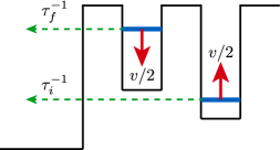
Figure 1: (Color online) (a) Illustration of the Landau-Zener transition between two levels, $i$ and $f$, decaying into continuum. As the levels are swept by each other with relative velocity, $v$, an electron, initially in $i$, can tunnel into the state $f$ and back with the amplitude, $J$. The decay time, $\tau_{i}$, of the state $i$ is much longer than the decay time, $\tau_{f}$, of the state, $f$.

II Coupling of the levels i and f via the continuum

For concreteness we consider a realization of the Landau-Zener transition between the two tunnel-coupled quantum dots in which the levels are swept past each other by the gate voltage, see FIG. 1. As illustrated in the figure, the levels i and f are coupled to the same continuum. The Hamiltonian of the system reads

$${\hat{H}}=E_{i}(t)C_{i}^{\dagger}C_{i}+E_{f}(t)C_{f}^{\dagger}C_{f}+\sum_{\nu}\left(V_{\nu i}C_{\nu}^{\dagger}C_{i}+V_{i\nu}C_{i}^{\dagger}C_{\nu}\right)$$

$$+\sum_{\mu}\left(W_{\mu f}C_{\mu}^{\dagger}C_{f}+W_{f\mu}C_{f}^{\dagger}C_{\mu}\right)+J\left(C_{i}^{\dagger}C_{f}+C_{f}^{\dagger}C_{i}\right)$$

$$+\sum_{\nu}E_{\nu}C_{\nu}^{\dagger}C_{\nu},$$ (1)

where $C_{i}^{\dagger}$, $C_{f}^{\dagger}$, and $C_{\nu}^{\dagger}$ are the creation operators of electron in the initial and final states, and the state $\nu$ in the continuum; $E_{i}(t)=\frac{vt}{2}$ and $E_{f}(t)=-\frac{vt}{2}$ are the positions of the levels $i$ and $f$, while $E_{\nu}$ is the energy of the state $\nu$ in the continuum. Coupling constants $V_{\nu i}$ and $W_{\mu f}$ of the states $i$ and $f$ to continuum are assumed to be very different, $W_{\mu f}\gg V_{\nu i}$.

Denote with $\Psi_{i}({\bf r})$ and $\Psi_{f}({\bf r})$ the wavefunctions of the initial and final states, and with $\Psi_{\nu}({\bf r})$ the wavefunction of the state ${\nu}$ of the continuum. Searching for solution of the time-dependent Schrödinger equation in the formLarkin ; prigodin

$$\Psi({\bf r},t)=a_{i}(t)\Psi_{i}({\bf r})+a_{f}(t)\Psi_{f}({\bf r})+\sum_{\nu}a_{\nu}(t)\Psi_{\nu}({\bf r}),$$ (2)

we get the following system of equations for the amplitudes $a_{i}$, $a_{f}$, and $a_{\nu}$

$$i{\dot{a}_{i}}=\frac{vt}{2}a_{i}+Ja_{f}+\sum_{\nu}V_{i\nu}a_{\nu},$$

$$i{\dot{a}_{f}}=-\frac{vt}{2}a_{f}+Ja_{i}+\sum_{\mu}W_{f\mu}a_{\mu},$$

$$i{\dot{a}_{\nu}}=E_{\nu}a_{\nu}+V_{\nu i}a_{i}+W_{\nu f}a_{f}.$$ (3)

As a next step, we eliminate the states of the continuous spectrum from the system. For this purpose,prigodin we perform the Laplace transform: ${\overline{a}=\int_{0}^{\infty}dta(t)\exp(-pt)}$ of the system Eq. II. With initial conditions $a_{i}(0)=1$, $a_{f}(0)=1$, and $a_{\nu}(0)=0$, we find

$$i\left(-1+{\overline{a}_{i}}\right)=\frac{v}{2}\frac{\partial{\overline{a}_{i}}}{\partial p}+J{\overline{a}_{f}}+\sum_{\nu}V_{i\nu}{\overline{a}_{\nu}},$$

$$ip{\overline{a}_{f}}=-\frac{v}{2}\frac{\partial{\overline{a}_{f}}}{\partial p}+J{\overline{a}_{i}}+\sum_{\mu}W_{f\mu}{\overline{a}_{\mu}},$$

$$ip{\overline{a}_{\nu}}=E_{\nu}{\overline{a}_{\nu}}+V_{\nu i}{\overline{a}_{i}}+W_{\nu f}{\overline{a}_{f}}.$$ (4)

A closed system of equations for ${\overline{a}_{i}}$, ${\overline{a}_{f}}$ emerges upon expressing ${\overline{a}_{\nu}}$ from the third equation and substituting it into the first and second equations. This yields

$$-i+\left(ip-\sum_{\nu}\frac{V_{i\nu}V_{\nu i}}{ip-E_{\nu}}\right){\overline{a}_{i}}-\frac{v}{2}\frac{\partial{\overline{a}_{i}}}{\partial p}$$

$$=\left(J+\sum_{\nu}\frac{V_{i\nu}W_{\nu f}}{ip-E_{\nu}}\right){\overline{a}_{f}},$$ (5)

$$\left(ip-\sum_{\mu}\frac{W_{f\mu}W_{\mu f}}{ip-E_{\mu}}\right){\overline{a}_{f}}+\frac{v}{2}\frac{\partial{\overline{a}_{f}}}{\partial p}$$

$$=\left(J+\sum_{\mu}\frac{W_{f\mu}V_{\mu i}}{ip-E_{\mu}}\right){\overline{a}_{i}}.$$ (6)

When $V_{i\nu}$ and $W_{f\mu}$ depend on $\nu$ and $\mu$ only weakly, the sums over $\nu$ and $\mu$ can be replaced by $\frac{i}{\tau_{i}}$ and $\frac{i}{\tau_{f}}$, respectively, where $\tau_{i}$ and $\tau_{f}$ are defined as

$$\frac{1}{\tau_{i}}=2\pi\sum_{\nu}|V_{\nu i}|^{2}\delta(E_{\nu}-p^{\prime\prime}),$$

$$\frac{1}{\tau_{f}}=2\pi\sum_{\mu}|W_{\mu f}|^{2}\delta(E_{\mu}-p^{\prime\prime}).$$ (7)

He $p^{\prime\prime}$ is the imaginary part of $p$.

The meaning of the times $\tau_{i}$ and $\tau_{f}$ is the decay times from the states $i$ and $f$ into the continuum, respectively. Similarly to Eq. II, the sum in the right-hand sides that adds to $J$ can be cast in the form

$$\frac{1}{\tau_{if}}=2\pi\sum_{\nu}V_{i\nu}W_{\nu f}\delta(E_{\nu}-p^{\prime\prime}).$$ (8)

Inspection of the equations II and 8 leads to an important relation.shahbazyan

$$\tau_{if}=(\tau_{i}\tau_{f})^{1/2}.$$ (9)

This relation suggests that, under the assumption $\tau_{i}\gg\tau_{f}$, adopted above, the times $\tau_{if}$ and $\tau_{i}$ are related as $\tau_{if}\gg\tau_{i}$. Thus, the second-order process: coupling of the states $i$ and $f$ via the continuum plays a crucial role in the scenario of the Landau-Zener transition. Namely, in the course of the transition, we can neglect the decay of the state $i$. After the transition is completed, the survived particle will eventually escape into the continuum after the time $\tau_{i}$.

III Survival probability with coupling via the continuum

With the states of continuum integrated out, it is convenient to analyze the system of equations for $a_{i}$ and $a_{f}$ in the time domain where it takes the form

$$i\left({\dot{a}}_{i}+\frac{a_{i}}{\tau_{i}}\right)=-\frac{vt}{2}a_{i}+\left(J+\frac{i}{\tau_{if}}\right)a_{f},$$

$$i\left({\dot{a}}_{f}+\frac{a_{f}}{\tau_{f}}\right)=\frac{vt}{2}a_{f}+\left(J+\frac{i}{\tau_{if}}\right)a_{i}.$$ (10)

To proceed, we express $a_{f}$ from the first equation and substitute it into the second. Upon this substitution, we arrive to the closed equation for $a_{i}$

$${\ddot{a}}_{i}+{\dot{a}}_{i}\left(\frac{1}{\tau_{i}}+\frac{1}{\tau_{f}}\right)+a_{i}\Biggl{\{}\frac{iv}{2}+\Biggl{[}\frac{vt}{2}+\frac{i}{2}\left(\frac{1}{\tau_{i}}-\frac{1}{\tau_{f}}\right)\Biggr{]}^{2}+\frac{1}{4}\left(\frac{1}{\tau_{i}}+\frac{1}{\tau_{f}}\right)^{2}+\left(J+\frac{i}{\tau_{if}}\right)^{2}\Biggr{\}}=0.$$ (11)

Naturally, in the absence of decay, $\tau_{i},\tau_{f},\tau_{if}\rightarrow\infty$, this equation reduces to the conventional equation describing the Landau-Zener transition and yielding $\exp\left(-\frac{2\pi J^{2}}{v}\right)$ for the survival probability. With regard to the result of Refs. Akulin1992, , Vitanov1997, setting only two times, $\tau_{i}$ and $\tau_{if}$, out of three to infinity leaves the result, $\exp\left(-\frac{2\pi J^{2}}{v}\right)$, unchanged. To trace how this happens, we introduce instead of the amplitude $a_{i}(t)$ a new variable ${\cal A}_{i}(t)$ as follows

$$a_{i}(t)={\cal A}_{i}(t)\exp\Bigg{[}-\frac{t}{2}\left(\frac{1}{\tau_{i}}+\frac{1}{\tau_{f}}\right)\Bigg{]}.$$ (12)

Substitution Eq. 12 allows to eliminate the first derivative in Eq. 11 and to reduce it to the Schrödinger-like form. The result of the substitution reads

$${\ddot{\cal A}}_{i}=$$

$$-{\cal A}_{i}\Biggl{\{}\frac{iv}{2}+\Biggl{[}\frac{vt}{2}+\frac{i}{2}\left(\frac{1}{\tau_{i}}-\frac{1}{\tau_{f}}\right)\Biggr{]}^{2}+\left(J+\frac{i}{\tau_{if}}\right)^{2}\Biggr{\}}.$$ (13)

To get an idea how the short decay time, $\tau_{f}$, drops out from the survival probability, we make use of the fact that, in the long-time limit, the semiclassical approach applies. The semiclassical phase is given by

$$\Phi(t)=$$

$$\pm i\int\limits_{0}^{t}dt^{\prime}\Biggl{\{}\frac{iv}{2}+\Biggl{[}\frac{vt^{\prime}}{2}+\frac{i}{2}\left(\frac{1}{\tau_{i}}-\frac{1}{\tau_{f}}\right)\Biggr{]}^{2}+\left(J+\frac{i}{\tau_{if}}\right)^{2}\Biggr{\}}^{1/2}.$$ (14)

Keeping only two leading terms, in the long-time limit, we have $\Phi(t)\approx\pm i\left[\frac{vt^{2}}{4}-\frac{t}{2}\left(\frac{1}{\tau_{i}}-\frac{1}{\tau_{f}}\right)\right]$. The sign ”-” leads to a growing exponent $\propto\exp\left(\frac{t}{2\tau_{f}}\right)$ in ${\cal A_{i}}(t)$. This term is canceled by the prefactor in Eq. 12. This cancellation illustrates the message of Refs. Akulin1992, , Vitanov1997, about the dropout of the decay. Still, unlike Refs. Akulin1992, , Vitanov1997, , the decay $\propto\exp\left(-\frac{t}{2\tau_{i}}\right)$ with a long decay time survives in $a_{i}(t)$.

If, at long times, we view Eq. III as a Schrödinger equation, it can be seen that the corresponding energy is positive and equal to $J^{2}$ for $J\tau_{if}\gg 1$, a well-known result for the Landau-Zener transition. However, in the opposite limit, $J\tau_{if}\ll 1$, which corresponds to the strong coupling between $i$ and $f$ via the continuum, the energy in the effective Schrödinger equation is negative and is equal to $-\frac{1}{\tau_{if}^{2}}$. Having in mind that the potential in the effective Schrödinger equation Eq. III is the inverted parabola, we conclude that the electron passes the transition domain by tunneling. To trace how this nontrivial scenario unfolds, we reduce Eq. III to a standard form by introducing a new variable

$$z=v^{1/2}e^{\frac{\pi i}{4}}\Biggl{[}t+\frac{i}{v}\left(\frac{1}{\tau_{i}}-\frac{1}{\tau_{f}}\right)\Biggr{]}.$$ (15)

We see that the new variable absorbs the imaginary contribution to time, $t$. With a new variable, Eq. III reduces to a standard differential equation for the parabolic cylinder functionsBateman

$$\frac{d^{2}{\cal A}_{i}}{dz^{2}}+\left(\nu+\frac{1}{2}-\frac{z^{2}}{4}\right){\cal A}_{i}=0,$$ (16)

where the parameter $\nu$ is given by

$$\nu=-\frac{i}{v}\left(J+\frac{i}{\tau_{if}}\right)^{2}.$$ (17)

We see that, as a result of coupling via the continuum, the parameter $\nu$, describing the transition quantitatively, comes out to be complex.

Note that for a conventional Landau-Zener transition the parameter $\nu$ is given by $\nu=-\frac{iJ^{2}}{v}$ with a sign minus. To find out how the complex structure of $\nu$ is reflected in survival probability, we need to inspect the solutions of Eq. 16 at complex $\nu$. To do so, we start from the integral representation of the parabolic cylinder function

$$D_{\nu}(z)=\Bigl{(}\frac{2}{\pi}\Bigr{)}^{1/2}e^{\frac{z^{2}}{4}}\int\limits_{0}^{\infty}du~{}e^{-\frac{u^{2}}{2}}u^{\nu}\cos\left(zu-\frac{\pi\nu}{2}\right),$$ (18)

where the integrals $I_{\pm}(z)$ are defined as

$$I_{\pm}(z)=D_{\nu}(z)=\Bigl{(}\frac{1}{2\pi}\Bigr{)}^{1/2}e^{\frac{z^{2}}{4}}\int\limits_{0}^{\infty}du~{}u^{\nu}e^{-\frac{u^{2}}{2}\pm iuz}.$$ (19)

Following Ref. Zhuxi, , it is convenient to divide the integral Eq. (18) into two contributions

$$D_{\nu}(z)=I_{+}(z)e^{\frac{i\pi\nu}{2}}+I_{-}(z)e^{-\frac{i\pi\nu}{2}},$$ (20)

where the integrals $I_{\pm}(z)$ are defined as

$$I_{\pm}(z)=D_{\nu}(z)=\Bigl{(}\frac{1}{2\pi}\Bigr{)}^{1/2}e^{\frac{z^{2}}{4}}\int\limits_{0}^{\infty}du~{}u^{\nu}e^{-\frac{u^{2}}{2}\pm iuz},$$ (21)

so that $I_{+}(z)=I_{-}(-z)$. This suggests that the factors $e^{\frac{i\pi\nu}{2}}$ and $e^{-\frac{i\pi\nu}{2}}$ describe the relation of the amplitudes of the wave function at negative and positive times. Thus, in calculation of the ratio of intensities the imaginary part of $(J+\frac{i}{\tau_{if}})^{2}$ drops out. This leads us to the final result for the survival probability

$$\exp\Big{(}-\frac{2\pi}{v}{\Big{|}}J^{2}-\frac{1}{\tau_{if}^{2}}{\Big{|}}\Big{)}.$$ (22)

IV Concluding remarks

The prime message of the present manuscript pertains to the papers Sinitsyn2004, , Shytov, . According to these papers, the survival probability is determined by times much longer than the decay time, which leads to the conclusion that the decay of the final state does not affect the survival probability of the Landau-Zener transition. We point out that the above argument does not apply when the coupling of the initial and the final states via the continuum is taken into account. Replacing one final state by the multitude of states with coupling distributed between them emulates the broadening of the final state, and justifies inefficiency of this broadening for the survival probability. However, this trick does not capture the $\tau_{if}$ process. The ${\tau_{if}}$ process consisting of virtual transition of an electron from initial state into the continuum followed by virtual transition into the final state leads to the formation of the Landau-Zener gap, which is purely imaginary. Even in the absence of the real gap, $J$, this gap, $\frac{1}{\tau_{if}}$, determines the survival probability. However, after a long time, $\tau_{i}$, the electron that survived the transition still escapes into the continuum.

Note that the combination $J+\frac{i}{\tau_{if}}$ appeared earlier in Ref. shahbazyan, in relation to two-channel resonant tunneling.

It is instructive to compare our results with Ref. Rajesh, where the decay also enters into the survival probability. In Ref. Rajesh, the left and right localized states in FIG. 1 formed doublets. The states of the right doublet, emulating the initial state of the Landau-Zener transition, did not decay, while both states of the right doublet, emulating the final state, did decay into continuum. It was shown in Ref. Rajesh, , that, unlike the conventional transition, the decay rates of the final states entered the survival probability, if they are different. By contrast, in the present manuscript we consider a conventional Landau-Zener transition, but allow both mutually crossing levels to decay.

V Acknowledgement

R.K.M. would like to thank the U.S. Department of Energy, Office of Science, Basic Energy Sciences, Materials Sciences and Engineering Division, Condensed Matter Theory Program. R.K.M. was also supported by the Center for Nonlinear Studies.

References

- (1) L. D. Landau, “Zur theorie der energieubertragung,” Physics of the Soviet Union 2, 46 (1932).
- (2) C. Zener, “Non-adiabatic crossing of energy levels,” Proc. R. Soc. A 137 (833), 696 (1932).
- (3) E. Majorana, “Atomi orientati in campo magnetico variabile,” Il Nuovo Cimento 9 (2), 43 (1932).
- (4) E. C. G. Stueckelberg, “Theory of inelastic collisions between atoms,” Helv. Phys. Acta 5, 369 (1932).
- (5) P. Nalbach, M. Thorwart, “Landau-Zener Transitions in a Dissipative Environment: Numerically Exact Results,” Phys. Rev. Lett. 103, 220401 (2009).
- (6) P. Nalbach, M. Thorwart, “Landau-Zener transitions mediated by an environment: Population transfer and energy dissipation,” J. Chem. Phys. 140, 124709 (2014)
- (7) P. Nalbach, “Crossing time in the dissipative Landau–Zener quantum dynamics,” Eur. Phys. J. B 95, 41 (2022).
- (8) M. Wubs, K. Saito, S. Kohler, P. Hänggi, Y. Kayanuma, “Gauging a Quantum Heat Bath with Dissipative Landau-Zener Transitions,” Phys. Rev. Lett. 97, 200404 (2006).
- (9) V.L. Pokrovsky, D. Sun, “Fast quantum noise in the Landau-Zener transition,” Phys. Rev. B 76, 024310 (2007)
- (10) S. Javanbakht, P. Nalbach, M. Thorwart, “Dissipative Landau-Zener quantum dynamics with transversal and longitudinal noise,” Phys. Rev. A 91, 052103 (2015).
- (11) R.S. Whitney, M. Clusel, T. Ziman, “Temperature can enhance coherent oscillations at a Landau-Zener transition,” Phys. Rev. Lett. 107, 210402 (2011).
- (12) Z. Huang, Y. Zhao, “Dynamics of dissipative Landau-Zener transitions,” Phys. Rev. A 97, 013803 (2018).
- (13) R. K. Malla, E. G. Mishchenko, and M. E. Raikh, “Suppression of the Landau-Zener transition probability by weak classical noise,” Phys. Rev. B 96, 075419 (2017).
- (14) R.K. Malla, M.E. Raikh, “Landau-Zener transition in a two-level system coupled to a single highly excited oscillator,” Phys. Rev. B 97, 035428 (2018).
- (15) R. Chen, “Landau-Zener transitions in a fermionic dissipative environment,” Phys. Rev. B 101, 125426 (2020).
- (16) S. Ashhab, “Landau-Zener transitions in a two-level system coupled to a finite-temperature harmonic oscillator,” Phys. Rev. A 90, 062120 (2014)
- (17) S. Ashhab, “Landau-Zener transitions in an open multilevel quantum system ,” Phys. Rev. A 94, 042109 (2016).
- (18) O. V. Ivakhnenko, S. N. Shevchenko, and Franco Nori, “Quantum Control via Landau-Zener-Stückelberg-Majorana Transitions,” arXiv:2203.16348 (2022).
- (19) V. M. Akulin and W. P. Schleicht, “Landau-Zener transition to a decaying level,” Phys. Rev. A 46, 4110 (1992).
- (20) N. V. Vitanov and S. Stenholm, “Pulsed excitation of a transition to a decaying level,” Phys. Rev. A 55, 2982 (1997).
- (21) N. A. Sinitsyn, “Counterintuitive transitions in the multistate Landau-Zener problem with linear level crossings,” J. Phys. A: Math. Gen. 37, 10691 (2004).
- (22) A. V. Shytov, “Landau-Zener transitions in a multilevel system. An exact result,” Phys. Rev. A 70, 052708(2004).
- (23) A. I. Larkin and K. A. Matveev, “Current-voltage characteristics of mesoscopic semiconductor contacts,” JETP 66, 580 (1987) [ZhETF 93, 1030 (1987)].
- (24) V. N. Prigodin and M. E. Raikh, “Decay of the population of quasilocal states in disordered media,” Phys. Rev. B 43, 14073 (1991).
- (25) T. V. Shahbazyan and M. E. Raikh, “Two-channel resonant tunneling,” Phys. Rev. B 49, 17123 (1994).
- (26) Higher Transcendental Functions, edited by A. Erdelyi, Vol. 2 (McGraw-Hill, New York, 1953).
- (27) Zhu-Xi Luo and M. E. Raikh, “Landau-Zener transition driven by slow noise,” Phys. Rev. B 95, 064305 (2017).
- (28) R. K. Malla and M. E. Raikh, “Effect of decay of the final states on the probabilities of the Landau-Zener transitions in multistate non-integrable models,” arXiv:2204.11782.