Abstract

The group of compactly supported Hamiltonian diffeomorphisms of a symplectic manifold is endowed with a natural bi-invariant distance, due to Viterbo, Schwarz, Oh, Frauenfelder and Schlenk, coming from spectral invariants in Hamiltonian Floer homology. This distance has found numerous applications in symplectic topology. However, its diameter is still unknown in general. In fact, for closed symplectic manifolds there is no unifying criterion for the diameter to be infinite. In this paper, we prove that for any Liouville domain this diameter is infinite if and only if its symplectic cohomology does not vanish. This generalizes a result of Monzner-Vichery-Zapolsky and has applications in the setting of closed symplectic manifolds.

1 Introduction and results

Liouville domains are a special kind of compact symplectic manifolds with boundary. They are characterized by their exact symplectic form $\omega=\differential\lambda$ and the fact that their boundary is of contact type. Given that they do not close up, they are quite easy to construct and allow us to study under a common theoretical framework many important classes of symplectic manifolds. Examples of such manifolds include cotangent disk bundles over closed manifolds, complements of Donaldson divisors [Gir17], preimages of some intervals under exhausting functions of Stein manifolds [CE12], positive regions of convex hypersurfaces in contact manifolds [Gir91] and total spaces of Lefschetz fibrations.

A key invariant of a Liouville domain $D$ is its symplectic cohomology $\operatorname{SH}^{\ast}(D)$. It was first defined by Cielieback, Floer and Hofer [FH94, CFH95] and later developed by Viterbo [Vit99]. Symplectic cohomology allows one to study the behavior of periodic Reeb orbits on the boundary of $D$. It is defined in terms of the Floer cohomology groups of a specific class of Hamiltonian functions on the completion $\hat{D}$ of $D$ which results from the gluing of the cylinder $[1,\infty)\times\partial D$ to $\partial D$.

The primary goal of this paper is to relate symplectic cohomology and spectral invariants, an important characteristic in Hamiltonian dynamics. When defined on a symplectic manifold $(M,\omega)$, spectral invariants associate to any pair $(\alpha,H)\in\operatorname{H}^{\ast}(M)\times C_{c}^{\infty}(S^{1}\times M)$ a real number $c(\alpha,H)$, that belongs to the spectrum of the action functional associated to $H$. Spectral invariants were first defined in $\mathbb{R}^{2n}$ from the point of view of generating functions by Viterbo in [Vit92]. They were then constructed on closed symplectically aspherical manifolds by Schwarz in [Sch00] and general closed symplectic manifolds by Oh in [Oh05] (see also [Ush13]).

In [FS07], Frauenfelder and Schlenk construct spectral invariants on Liouville domains. These spectral invariants are homotopy invariant in the Hamiltonian term in the following sense. If two compactly supported Hamiltonians $H$ and $F$ generate the same time-one map, $\varphi_{H}=\varphi_{F}$, then $c(\alpha,H)=c(\alpha,F)$. Thus $c(\alpha,\bullet)$ descends to the group of compactly supported Hamiltonian diffeomorphisms $\operatorname{Ham}_{c}(D)$. This allows one to define a bi-invariant norm $\gamma$ on $\operatorname{Ham}_{c}(D)$, called the spectral norm, by

$$\gamma(\varphi)=c(1,\varphi)+c(1,\varphi^{-1})$$ .

One key feature of the spectral norm $\gamma$ is the fact that it acts as a lower bound to the celebrated Hofer norm introduced by Hofer in [Hof90] (see the article of Lalonde and McDuff [LM95] and the book of Polterovich [Pol01] for further developments in the subject). It is thus natural to ask whether the spectral diameter

$$\operatorname{diam}_{\gamma}(M)=\sup\{\gamma(\varphi)\mid\varphi\in\operatorname{Ham}_{c}(M)\}$$

is finite or not. In particular, if $\operatorname{diam}_{\gamma}(M)=+\infty$ then the Hofer norm is assured to be unbounded. Further links between the spectral norm and Hofer geometry are discussed in Section 1.4.

1.1 Main results

In this article, we find a characterization of the finiteness of $\operatorname{diam}_{\gamma}(D)$ in the case of a Liouville domain $(D,\differential\lambda)$ in terms of its symplectic cohomology.

Our main technical result shows that if $\operatorname{SH}^{\ast}(D)\neq 0$ then $c(1,H)$ can be made arbitrarily large. This, combined with the converse implication which was proved by Benedetti and Kang [BK], implies

Theorem A1.

Let $(D,\lambda)$ be a Liouville domain. Then $\operatorname{diam}_{\gamma}(D)=+\infty$ if and only if $\operatorname{SH}^{\ast}(D)\neq 0$.

As an intermediate step to proving Theorem A1, we show the following auxiliary result.

Lemma B.

Let $H$ be a compactly supported Hamiltonian on a Liouville domain $(D,\lambda)$. Then,

$$c(1,H)\geq 0.$$

Lemma B is a cohomological adaptation of [GT, Lemma 4.1].

In fact, when the symplectic cohomology of a Liouville domain is non-vanishing, the implication of Theorem A1 follows from a sharper result. Denote by $d_{\gamma}(\varphi,\psi)=\gamma(\varphi\circ\psi^{-1})$ the spectral distance on $\operatorname{Ham}_{c}(D)$ and by $d_{\text{{st}}}$ the standard Euclidean distance on $\mathbb{R}$.

Theorem A2.

Let $(D,\lambda)$ be a Liouville domain such that $\operatorname{SH}^{\ast}(D)\neq 0$. Then there exists an isometric group embedding $(\mathbb{R},d_{\text{st}})\to(\operatorname{Ham}_{c}(D),d_{\gamma})$.

The proof of Theorem A2 uses an explicit construction of an isometric group embedding. This construction is a generalization of the procedure used by Monzner and Vichery and Zapolsky to prove Theorem 3 below. The construction of the aforementioned embedding relies primarily on the computation of spectral invariants of Hamiltonians which are constant on the skeleton of $D$, a special subset of Liouville domains which we define in Section 2.1.

Lemma C.

Suppose $(D,\lambda)$ is a Liouville domain such that $\operatorname{SH}^{\ast}(D)\neq 0$. Let $H$ be a compactly supported autonomous Hamiltonian on $D$ such that

$$H\big{|}_{\operatorname{Sk}(D)}=-A\quad\text{and}\quad-A\leq H\big{|}_{D}\leq 0$$

for a constant $A>0$. Then

$$c(1,H)=A.$$

1.2 What is already known for Liouville domains

Following the work of Benedetti and Kang [BK], it is known that the spectral diameter of a Liouville domain $D$ is bounded if its symplectic cohomology vanishes. This result was achieved using a special capacity derived from the filtered symplectic cohomology of $D$. To better understand how this is done, let us give an overview of the construction of $\operatorname{SH}^{*}(D)$ following [Vit99].

Focusing our attention to the class of Hamiltonians, called admissible, which are affine in the radial coordinate on the cylindrical part of $\hat{D}$, filtered cohomology groups $\operatorname{HF}_{(a,b)}^{\ast}(H)$ are well defined and only depend on the slope of the Hamiltonian on $[1,\infty)\times\partial D$. Taking an increasing sequence of admissible Hamiltonians $\left\{H_{i}\right\}_{i}$ with corresponding slopes $\left\{\tau_{i}\right\}_{i}$ satisfying $\tau_{i}\to+\infty$, one can define the filtered symplectic cohomology $\operatorname{SH}_{(a,b)}^{\ast}(D)$ of $D$ as

$$\operatorname{SH}_{(a,b)}^{\ast}(D)=\lim_{\begin{subarray}{c}\longrightarrow\\ H_{i}\end{subarray}}\operatorname{HF}_{(a,b)}^{\ast}(H_{i}).$$

It follows from the above definition that for $a\leq a^{\prime}$ and $b\leq b^{\prime}$ there is a natural map $\iota_{a,a^{\prime}}^{b,b^{\prime}}:\operatorname{SH}_{(a,b)}^{\ast}(D)\to\operatorname{SH}_{(a^{\prime},b^{\prime})}^{\ast}(D)$. Moreover, the full symplectic cohomology $\operatorname{SH}^{\ast}(D)=\operatorname{SH}_{(-\infty,\infty)}^{\ast}(D)$ comes with a natural map

$$v^{\ast}:\operatorname{H}^{\ast}(D)\to\operatorname{SH}^{\ast}(D).$$

called the Viterbo map. The failure of $v^{\ast}$ to be an isomorphism signals the presence of Reeb orbits on the boundary of $D$. Thus, $\operatorname{SH}^{\ast}(D)$ is a useful tool to study the Weinstein conjecture [Wei79] which claims that on any compact contact manifold, the Reeb vector field should admit at least one periodic orbit. For instance, in [Vit99], Viterbo proves the Weinstein conjecture for the boundary of subcritical Stein manifolds. Note that the symplectic cohomology approach to the Weinstein conjecture has limitations as it relies on finding a Liouville filling of the given contact manifold.

We can extend any compactly supported Hamiltonian $H\in C_{c}^{\infty}(S^{1}\times D)$ to an admissible Hamiltonian with small slope $H^{\varepsilon}$ and define its Floer cohomology as $\operatorname{HF}^{\ast}(H)=\operatorname{HF}^{\ast}(H^{\varepsilon})$. A key property of Floer cohomology on Liouville domains is that if an admissible Hamiltonian $F$ has a slope close enough to zero, then we have an isomorphism $\Phi_{F}:\operatorname{H}^{\ast}(D)\to\operatorname{HF}^{\ast}(F)$. Thus, the Floer cohomology of compactly supported Hamiltonians on $D$ is well defined.

Let $H$ be a compactly supported Hamiltonian. Followig [FS07], the spectral invariant associated to $(\alpha,H)\in\operatorname{H}^{\ast}(D)\times C_{c}^{\infty}(S^{1}\times D)$ corresponds to the real number

$$c(\alpha,H)=\inf\left\{c\in\mathbb{R}\mid\Phi_{H}(\alpha)\in\operatorname{im}\iota^{<c}\right\}$$

where

$$\iota^{<c} =\iota_{-\infty,-\infty}^{c,+\infty}:\operatorname{HF}_{(-\infty,c)}^{\ast}(H)\to\operatorname{HF}^{\ast}(H)$$

is the map induced by natural inclusion of subcomplexes.

Now, define the SH-capacity of $D$ as

$$c_{\operatorname{SH}} (D)=\inf\left\{c>0\mid\iota_{-\infty,-\infty}^{\varepsilon,c}=0\right\}\in(0,\infty],$$

where, for $\epsilon>0$ sufficiently small, $\iota_{-\infty,-\infty}^{\varepsilon,c}:\operatorname{SH}_{(-\infty,\varepsilon)}^{\ast}(D)\to\operatorname{SH}_{(-\infty,c)}^{\ast}(D)$. It is known that $c_{\text{SH}}(D)$ is finite if and only if $\operatorname{SH}^{\ast}(D)$ vanishes. Using this, Benedetti and Kang prove the following upper bound on spectral invariants of compactly supported Hamiltonians with respect to the unit.

Theorem 1 ([BK]).

Let $(D,\differential\lambda)$ be a Liouville domain with $\operatorname{SH}^{\ast}(D)=0$. Then,

$$\sup\{c(1,H)\}\leq c_{\operatorname{SH}}(D)<+\infty,$$

where the supremum is taken over all compactly supported Hamiltonians in $D$.

In particular, by definition of the spectral norm, if $\operatorname{SH}^{\ast}(D)=0$, then for any compactly supported Hamiltonian $H$ generating $\varphi_{H}\in\operatorname{Ham}_{c}(D)$, we have

$$\gamma(\varphi) =c(1,\varphi)+c(1,\varphi^{-1})\leq 2c_{\operatorname{SH}}(D)<+\infty.$$

Therefore, Theorem 1 provides the only if part of Theorem A1.

On the other hand, symplectic cohomology is known to be non-zero in many cases [Sei08, Section 5]. Since we will be using $\mathbb{Z}_{2}$ coefficients throughout this article, one case of particular interest to us is the following.

Proposition 2 ([Vit99]).

Suppose $D$ contains a closed exact Lagrangian submanifold $L$. Then, $\operatorname{SH}^{\ast}(D)\neq 0$.

This result of Viterbo can be used, in conjunction with Theorem A1, to prove that the spectral diameter is infinite for quite general classes of Liouville domains.

1.2.1.  Cotangent bundles

In [MVZ12], Monzner, Vichery and Zapolsky show the following.

Theorem 3.

Let $N$ be a closed manifold. There exists an isometric group embedding of $(\mathbb{R},d_{\text{st}})$ in $(\operatorname{Ham}_{c}(T^{\ast}N),d_{\gamma})$.

For the reader’s convenience, we give a detailed proof of Theorem 3 along the lines of [MVZ12]. We refer the reader to Section 4 for details on the standard notation in use here.

Fix $H\in C_{c}^{\infty}(T^{\ast}N)$ such that $H|_{N}=1$ and $0\leq H\leq 1$. Let $\iota:\mathbb{R}\to\operatorname{Ham}_{c}(T^{\ast}N)$ be the map defined by

$$\iota(s)=\varphi_{sH}$$

where $\varphi_{sH}\in\operatorname{Ham}_{c}(T^{\ast}N)$ is the time-one map associated to $sH\in C_{c}^{\infty}(T^{\ast}N)$. We claim that $\iota$ is the desired embedding.

We first bound $d_{\gamma}(\iota(s),\iota(s^{\prime}))$ from above. As previously mentioned, if $F\in C_{c}^{\infty}(T^{\ast}N)$, then $\gamma(\varphi_{F})\leq\norm{F}$, where $\norm{F}=\max\absolutevalue{F}$ denotes the $C^{0}$-norm of $F$. Moreover, since $H$ is autonomous, $sH\#\overline{{s^{\prime}H}}=(s-s^{\prime})H$. Therefore,

$$d_{\gamma}(\iota(s),\iota(s^{\prime})) =\gamma(\iota(s)\iota(s^{\prime})^{-1})\leq\norm{(s-s^{\prime})H}=\absolutevalue{s-s^{\prime}}.$$

Now, we bound $d_{\gamma}(\iota(s),\iota(s^{\prime}))$ from below. In [MVZ12, Section 2] a Lagrangian spectral invariant $\ell(1,\bullet)$ with respect to the zero section $N$ of $T^{\ast}N$ is constructed. It is shown that $\ell(1,\bullet)\leq c(1,\bullet)$. One key property of $\ell(1,\bullet)$ is that if $F|_{N}=r$ for a constant $r\in\mathbb{R}$, then $\ell(1,F)=r$. Thus, by definition of $H$ and Lemma B, we have

$$d_{\gamma}(\iota(s),\iota(s^{\prime}))=c(1,(s-s^{\prime})H)+c(1,(s^{\prime}-s)H)\geq c(1,(s-s^{\prime})H).$$

and by the properties of $\ell(1,\bullet$),

$$d_{\gamma}(\iota(s),\iota(s^{\prime}))\geq\ell(1,(s-s^{\prime})H)=s-s^{\prime}.$$

In an analogous fashion, we obtain $d_{\gamma}(\iota(s),\iota(s^{\prime}))\geq s^{\prime}-s$. We can therefore conclude that

$$d_{\gamma}(\iota(s),\iota(s^{\prime}))\geq\absolutevalue{s-s^{\prime}}$$

as desired. This completes the proof.

Theorem 3 immediately implies

Corollary 4.

Let $N$ be a closed manifold. Then $\operatorname{diam}_{\gamma}(DT^{\ast}N)=+\infty$ .

To prove Corollary 4, one does not need the Lagrangian spectral norm. Indeed, since the zero section $N\subset DT^{\ast}N$ is an exact closed Lagrangian submanifold, Corollary 4 follows directly from Proposition 2 and Theorem A1.

1.3 The spectral diameter of other symplectic manifolds

It has been known for a long time [EP03] that for $(\mathbb{C}P^{n},\omega_{\text{FS}})$,

$$\operatorname{diam}_{\gamma}(\mathbb{C}P^{n})\leq\int_{\mathbb{C}P^{1}}\omega_{\text{FS}}$$ .

The above upper bound was latter optimized by Kislev and Shelukhin in [KS21, Theorem G] to

$$\operatorname{diam}_{\gamma}(\mathbb{C}P^{n})=\frac{n}{n+1}\int_{\mathbb{C}P^{1}}\omega_{\text{FS}}.$$

However, for a surface $\Sigma_{g}$ of genus $g\geq 1$, the spectral diameter is infinite. This case is covered by the following theorem of Kislev and Shelukhin [KS21, Theorem D] which is a sharpening of a result of Usher [Ush13, Theorem 1.1].

Theorem 5.

Let $(M,\omega)$ be a closed symplectic manifold that admits an autonomous Hamiltonian $H\in C^{\infty}(M,\mathbb{{R}})$ such that

• all the contractible periodic orbits of $X_{H}$ are constant.

Then $\operatorname{diam}_{\gamma}(M)=+\infty$.

Theorem 5 allows one to prove that the spectral diameter is infinite in many cases. A list of examples in which condition U1 holds can be found in [Ush13, Section 1]. As mentioned above, surfaces of positive genus satisfy U1. Also, if $(N,\omega_{N})$ satisfies U1 then so does $(M\times N,\omega_{M}\oplus\omega_{N})$ for any other closed symplectic manifold $(M,\omega_{M})$.

In [Kawb], Kawamoto proves that the spectral diameter of the quadrics $Q^{2}$ and $Q^{4}$ (of real dimension 4 and 8 respectively) and certain stabilizations of them is infinite.

1.3.1.  Symplectically aspherical manifolds

Recall that a symplectic manifold $(M,\omega_{M})$ is symplectically aspherical if both $\omega_{M}$ and the first Chern class $c_{1}(M)$ of $M$ vanish on $\pi_{2}(M)$, namely, for every continuous map $f:S^{2}\to M$,

$$\langle[\omega_{M}],f_{\ast}[S^{2}]\rangle=0=\langle c_{1}(M),f_{\ast}[S^{2}]\rangle.$$

An open subset $U\subset M$ is said to be incompressible if the map $\pi_{1}(U)\to\pi_{1}(M)$ induced by the inclusion is injective.

As pointed out in [BHS21], it has been conjectured that $\operatorname{diam}_{\gamma}(M)=+\infty$ on all closed symplectically aspherical manifolds. Here, we prove that conjecture in the case of the twisted product $(M\times M,\omega\oplus-\omega)$ of a closed symplectically aspherical manifold $(M,\omega)$ with itself. But first, a more general result.

Proposition D.

Let $(M,\omega)$ be a closed symplectically aspherical manifold of dimension $2n$. Suppose there exists an incompressible Liouville domain $D$ of codimension $0$ embedded inside $M$ with $SH^{\ast}(D)\neq 0$. Then, $\operatorname{diam}_{\gamma}(M)=+\infty$.

Proof.

Let $H$ be a compactly supported Hamiltonian in $D$ and denote by $\iota:D\to M$ the embedding. By a cohomological analogue of [GT, Claim 5.2], we have that

$$c_{D}(\beta,H)=\max_{\begin{subarray}{c}\alpha\in\operatorname{H}^{\ast}(M)\\ \iota^{\ast}(\alpha)=\beta\end{subarray}}c_{M}(\alpha,H)$$

for all $\beta\in\operatorname{H}^{\ast}(D)$ where $c_{D}$ and $c_{M}$ are the spectral invariants on $D$ and $M$ respectively. In particular, we know that the unit $1_{M}\in\operatorname{H}^{\ast}(M)$ is sent to the unit $1_{D}\in\operatorname{H}^{\ast}(D)$ under the map $\iota^{\ast}:\operatorname{H}^{\ast}(M)\to\operatorname{H}^{\ast}(D)$. Moreover, it is well known that the spectral invariant with respect to the unit can be implicitly written as

$$c_{M}(1_{M},H)=\max_{\alpha\in\operatorname{H}^{\ast}(M)}c_{M}(\alpha,H)$$

(see Lemma 26). Therefore, fixing $\beta=1_{D}$, we have

$$c_{D}(1_{D},H)=c_{M}(1_{M},H).$$

Using Theorem A1, the above equation thus yields the desired result. ∎

Corollary E.

Let $(M,\omega)$ be a closed symplectically aspherical manifold. Then, $\operatorname{diam}_{\gamma}(\operatorname{Ham}(M\times M,\omega\oplus-\omega))=+\infty$.

Proof.

Consider the closed Lagrangian given by the diagonal $L=\Delta$ inside $(M\times M,\omega_{M}\oplus-\omega_{M})$. In virtue of the Weinstein neighborhood theorem, there exists an open neighborhood $U$ of $L$ and a symplectomorphism $\psi:U\to D_{\varepsilon}T^{\ast}L$ such that $\varphi(L)$ coincides with the zero section of an $\epsilon$-radius codisk bundle $D_{\varepsilon}T^{\ast}L$ over $L$. The Liouville structure on $D_{\varepsilon}T^{\ast}L$ pulls back to a Liouville structure on $U$. Note that, inside $M\times M$, $L$ is incompressible, i.e. the map $\pi_{1}(L)\to\pi_{1}(M\times M)$ of first homotopy groups induced by the inclusion $L\to M\times M$ is injective. Therefore, by homotopy equivalence, $U$ and $D_{\varepsilon}T^{\ast}L$ are also incompressible. The desired result follows directly from Proposition D. ∎

1.4 Hofer geometry

As hinted at above, the finiteness of the spectral diameter plays a role in Hofer geometry. In particular, it can be used to study the following question posed by Le Roux in [LR10]:

Question 1. For any $A>0$, let

$$E_{A}(M,\omega):=\left\{\varphi\in\operatorname{Ham}(M,\omega)\mid d_{H}(\text{Id},\varphi)>A\right\}$$

be the complement of the closed ball of radius $A$ in Hofer’s metric. For all $A>0$, does $E_{A}(M,\omega)$ have non-empty $C^{0}$-interior?

Indeed, in the case of closed symplectically aspherical manifolds with infinite spectral diameter, a positive answer to Question 1 was given by Buhovsky, Humilière and Seyfaddini (see also [Kawa, Kawb] for the positive and negative monotone cases).

Theorem 6 ([BHS21]).

Let $(M,\omega)$ be a closed, connected and symplectically aspherical manifold. If $\operatorname{diam}_{\gamma}(M)=+\infty$, then $E_{A}(M,\omega)$ has non-empty $C^{0}$-interior for all $A>0$.

Using Theorem 6 in conjunction with Corollary E, we directly obtain the following answer to Question 1.4 in the specific setting of Corollary E.

Corollary F.

Let $(M,\omega)$ be a closed symplectically aspherical manifold. Then, $E_{A}(M\times M,\omega\oplus-\omega)$ has a non-empty $C^{0}$-interior for all $A>0$.

Acknowledgements

This research is a part of my PhD thesis at the Université de Montréal under the supervision of Egor Shelukhin. I thank him for proposing this project and outlining the approach used to carry it out in this paper. I am deeply indebted to him for the countless valuable discussions we had regarding spectral invariants and symplectic cohomology. I would also like to thank Octav Cornea and François Lalonde for their comments on an early draft of this project. I thank Leonid Polterovich, Felix Schlenk and Shira Tanny for their comments which helped improve the exposition. Finally, I am grateful to Marcelo Atallah, Filip Brocic, François Charette, Jean-Philippe Chassé, Dustin Connery-Grigg, Jonathan Godin, Jordan Payette and Dominique Rathel-Fournier for fruitful conversations. This research was partially supported by Fondation Courtois.

2 Liouville domains and admissible Hamiltonians

In this subsection we recall the definition of Liouville domains, specify the class of Hamiltonians we will restrict our attention to and describe how their Floer trajectories behave at infinity.

2.1 Completion of Liouville domains

A Liouville domain $(D,\differential\lambda,Y)$ is an exact symplectic manifold with boundary on which the vector field $Y$, defined by $Y\mathbin{\scalebox{1.2}{$\lrcorner$}}\differential\lambda=\lambda$ and called the Liouville vector field, points outwards along $\partial D$. Denote by $\hat{D}=D\cup[1,\infty)\times\partial D$ the completion of $D$ and $(r,x)$ the coordinates on $[1,\infty)\times\partial D$. Here, we glue $\partial D$ and $\left\{1\right\}\times\partial D$ with respect to the reparametrization $\psi_{Y}^{\ln r}$ of the Liouville flow generated by $Y$. Given $\delta>0$, let

$$D^{\delta} =\psi_{Y}^{\ln\delta}(D)=D\setminus(\delta,\infty)\times\partial D.$$

We extend the Liouville form $\lambda$ to $\hat{D}$ by defining $\hat{\lambda}:T\hat{D}\to\mathbb{R}$ as

$$\hat{\lambda}\mid_{D}\,=\lambda \quad\text{and}\quad\hat{\lambda}\mid_{\hat{D}\setminus D}\,=r\alpha$$

where $\alpha=\lambda|_{\partial D}$. The cylindrical portion $[1,\infty)\times\partial D$ of $\hat{D}$ is thus equipped with the symplectic form $\omega=\differential(r\alpha)$.

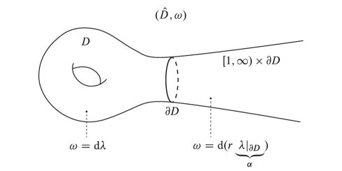
Figure 2.1: A Liouville domain.

The skeleton $\operatorname{Sk}(D)$ of $(D,\differential\lambda,Y)$ is defined by

$$\operatorname{Sk}(D)=\bigcap_{0<r<1}\psi_{Y}^{\ln r}(D).$$

Denote by $R_{\alpha}$ the Reeb vector field on $\partial D$ associated to $\alpha$, meaning

$$R_{\alpha}\mathbin{\scalebox{1.2}{$\lrcorner$}}\differential\alpha=0,\quad \alpha(R)=1.$$

We define $\operatorname{Spec}(\partial D,\alpha)$ to be the set of periods of closed characteristics, the periodic orbits generated by $R_{\alpha}$, on $\partial D$ and put

$$T_{0}=\min\operatorname{Spec}(\partial D,\lambda).$$

As a subset of $\mathbb{R}$, $\operatorname{Spec}(\partial D,\alpha)$ is known to be closed and nowhere dense. For any $A\in\mathbb{R}$, let $\eta_{A}$ denote the distance between $A$ and $\operatorname{Spec}(\partial D,\lambda)$.

2.2 Admissible Hamiltonians and almost complex structures

2.2.1.  Periodic orbits and action functional

Given a Hamiltonian $H:S^{1}\times\hat{D}\to\mathbb{R}$, one defines its time-dependent Hamiltonian vector field $X_{H}^{t}:\hat{D}\to T\hat{D}$ by

$$X_{H}^{t} \mathbin{\scalebox{1.2}{$\lrcorner$}}\omega=-dH_{t}$$

where $H_{t}(p)=H(t,p)$. We denote by $\varphi_{H}^{t}:\hat{D}\to\hat{D}$ the flow generated by $X_{H}^{t}$. The set of all contractible 1-periodic orbits of $\varphi_{H}^{t}$ is denoted by $\mathcal{P}(H)$. An orbit $x\in\mathcal{P}(H)$ is said to be non-degenerate if

$$\det(\mathrm{id}-d_{x(0)}\varphi_{H}^{1})\neq 0$$

and transversally non-degenerate if the eigenspace associated to the eigenvalue 1 of the map $d_{x(0)}\varphi^{1}$ is of dimension 1. If all elements of $\mathcal{P}(H)$ are non-degenerate or transversally non-degenerate, we say that $H$ is regular.

Let $\mathcal{L}\hat{D}$ be the space of contractible loops in $\hat{D}.$ For a Hamiltonian $H:S^{1}\times\hat{D}\to\mathbb{R}$ , the Hamiltonian action functional $\mathcal{A}_{H}:\mathcal{L}\hat{D}\to\mathbb{R}$ associated to $H$ is defined as

$$\mathcal{A}_{H}(x)= \int_{0}^{1}x^{\ast}\hat{\lambda}-\int_{0}^{1}H_{t}(x(t))\>\differential t.$$

It is well known that the elements elements of $\mathcal{P}(H)$ correspond to the critical points of $\mathcal{A}_{H}$, see [AD14, section 6]. The image of $\mathcal{P}(H)$ under the Hamiltonian action functional is called the action spectrum of $H$ and is denoted by $\operatorname{Spec}(H)$.

2.2.2.  Admissible Hamiltonians

The completion of a Liouville domain is obviously non-compact. We thus need to control the behavior at infinity of Hamiltonians we use in order for them to have finitely many 1-periodic contractible orbits.

Definition 7.

Let $r_{0}>1$. A Hamiltonian $H$ is $r_{0}$-admissible if

• $H(t,x,r)=h(r)$ on $\hat{D}\setminus D$,

• $h(r)$ is $C^{2}$-small on $(1,r_{0})$,

• $h(r)=\tau_{H}r-\tau_{H}r_{0}$ on $(r_{0},+\infty)$ for $\tau_{H}\in(0,\infty)\setminus\operatorname{Spec}(\partial D,\alpha)$,

• $H$ is regular.

We denote the set of such Hamiltonians $\mathcal{H}_{r_{0}}$.

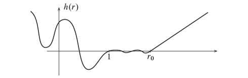
Figure 2.2: An $r_{0}$-admissible Hamiltonian.

We will also consider the set $\mathcal{H}_{r_{0}}^{0}\subset\mathcal{H}_{r_{0}}$ of $r_{0}$-admissibe Hamiltonians which are negative on $D$. In some cases, it is not necessary to specify $r_{0}$ as long as it is greater than $1$. For that purpose, we define

$$\mathcal{H}=\bigcup_{r_{0}>1}\mathcal{H}_{r_{0}},\quad\mathcal{H}^{0}=\bigcup_{r_{0}>1}\mathcal{H}_{r_{0}}^{0}.$$

Remark 8.

Suppose $H\in\mathcal{H}$. If $x\in\mathcal{P}(H)\cap\hat{D}\setminus D$ is non constant, then it is necessarily transversally non-degenerate. Indeed, since $H$ is time-independent there by definition, for any $c\in\mathbb{R}$, $x(t-c)$ is also a 1-periodic orbit of $H$.

Lemma 9.

If $H\in\mathcal{H}$, then $\absolutevalue{\mathcal{P}(H)}$ consists of a finite number of periodic orbits and $S^{1}$ families of periodic orbits.

Proof.

Since $D$ is compact, there is a finite number of 1-periodic orbits of $H$ inside it.

Next, we look at the elements of $\mathcal{P}(H)$ which sit inside $\hat{D}\setminus D$. On this subset of $\hat{D}$, we know that $H=h(r)$ and $\omega=\differential\hat{\lambda}$. Therefore, on $\hat{D}\setminus D$

$$X_{H}\mathbin{\scalebox{1.2}{$\lrcorner$}}\omega =X_{H}\mathbin{\scalebox{1.2}{$\lrcorner$}}(\differential r\wedge\alpha+r\differential\alpha)$$

$$=\differential r(X_{H})\alpha-\alpha(X_{H})\differential r+rX_{H}\mathbin{\scalebox{1.2}{$\lrcorner$}}\differential\alpha$$

and $\differential H=h^{\prime}(r)\differential r$. Hamilton’s equation thus yields

$$\differential r(X_{H})=0=X_{H}\mathbin{\scalebox{1.2}{$\lrcorner$}}\differential\alpha,\quad\alpha(X_{H})=h^{\prime}(r).$$

The three equations above imply the following two facts,

• on $\hat{D}\setminus D$, $X_{H}=h^{\prime}(r)R_{\alpha}$;

• if $x\in\mathcal{P}(H)$ is such that $x\cap\hat{D}\setminus D\neq\varnothing$, then $x\subset\left\{r\right\}\times\partial D$ for some $r>1$.

We conclude that a 1-periodic orbit $x$ of $H$ which lies inside $\{r\}\times\partial D$ corresponds to a Reeb orbit of period $h^{\prime}(r)$. Notice that since $\tau_{H}\notin(0,+\infty)\cap\operatorname{Spec}(\partial D,\alpha)$, $\mathcal{P}(H)\cap(\hat{D}\setminus D)=\mathcal{P}(H)\cap(D^{r_{0}}\setminus D)$. Moreover, $\operatorname{Spec}(\partial D,\alpha)$ being nowhere dense and closed in $\mathbb{R}$, we have that $\operatorname{Spec}(\partial D,\alpha)\cap(1,r_{0})$ is a finite set. We can therefore conclude, since every non-constant 1-periodic orbit of $H$ in $\hat{D}\setminus D$ is transversally non-degenerate, that $\mathcal{P}(H)\cap(\hat{D}\setminus D)$ consists of a finite number of $S^{1}$ families of periodic orbits. ∎

Remark 10.

The fact that admissible Hamiltonians are radial on the cylindrical part of $\hat{D}$ allows us to express the action of the 1-periodic orbits inside $\hat{D}\setminus D$ in terms of that radial function. To see this, we fix $H\in\mathcal{H}$ and compute the action of a non constant orbit $x\in\mathcal{P}(H)\cap(\hat{D}\setminus D)$ which we suppose lies inside $\{r\}\times\partial D$ for $r>1$:

$$\mathcal{A}_{H}(x) =\int_{0}^{1}x^{\ast}\hat{\lambda}-\int_{0}^{1}H\circ x\>\differential t$$

$$=\int_{0}^{1}r\alpha(X_{H})\differential t-\int_{0}^{1}h(r)\differential t=rh^{\prime}(r)-h(r).$$

The function $A_{H}(r)=rh^{\prime}(r)-h(r)$ on the right hand side of the above equation has a nice geometric interpretation. On the graph of $h$, $A_{H}(r^{\prime})$ corresponds to minus the $y$-coordinate of the intersection of the tangent at the point $(r^{\prime},h(r^{\prime}))$ and the $y$-axis.

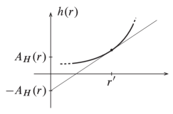
Figure 2.3: Action value of a periodic orbit contained in $\{r^{\prime}\}\times\partial D$.

2.2.3.  Monotone homotopies

We will need to also restrict the types of Hamiltonian homotopies we consider to the following class.

Definition 11.

Let $H_{s}=\left\{H_{s}\right\}_{s\in\mathbb{R}}$ be a smooth homotopy from $H_{+}\in\mathcal{H}_{r_{0}}$ to $H_{-}\in\mathcal{H}_{r_{0}^{\prime}}$ We say that $H_{s}$ is a monotone homotopy if the following conditions hold

• $\exists S>0$ such that $H_{s^{\prime}}=H_{-}$ for $s^{\prime}<-S$ and $H_{s^{\prime}}=H_{+}$ for $s^{\prime}>S$,

• $H_{s}=h_{s}(r)$ on $\hat{D}\setminus D$,

• for $R=\max\{r_{0},r_{0}^{\prime}\}$, $h_{s}(r)=\tau_{s}r+\eta_{s}$ on $(R,+\infty)$ for smooth functions $\tau_{s}$ and $\eta_{s}$ of $s$ and $\partial_{s}\tau_{s}\leq 0$.

For $H_{+}\in\mathcal{H}_{r_{0}}$ and $H_{-}\in\mathcal{H}_{r_{0}^{\prime}}$ with $\tau_{H_{+}}=\tau_{+}\leq\tau_{-}=\tau_{H_{-}}$, we can explicitly construct a monotone homotopy in the following way. Fix a positive constant $S>0$. Let $\beta:\mathbb{R}\to[0,1]$ be a smooth function such that $\beta(s)=0$ for $s\leq-S$, $\beta(s)=1$ for $s\geq S$ and $\beta^{\prime}(s)>0$ for all $s\in(-S,S)$. Define

$$H_{s} =H_{-}+\beta_{s}(H_{+}-H_{-}).$$

For $R=\max\left\{r_{0},r_{0}^{\prime}\right\}$ we have, on $\hat{D}\setminus D^{r_{0}}$,

$$H_{s}(t,r,p) =(\beta(s)(\tau_{+}-\tau_{-})+\tau_{-})r+\beta(s)(\eta_{+}-\eta_{-})+\eta_{-}$$

and $\partial_{s}\tau_{s}\leq 0$ as desired.

2.2.4.  Admissible almost complex structures

Let $J$ be an almost complex structure on $\hat{D}$. Recall that $J$ is $\omega$-compatible if the map $g_{J}:TM\otimes TM\to\mathbb{R}$ defined by

$$g_{J}(v,w) =\omega(v,Jw)$$

is a Riemannian metric. To control the behavior of $\omega$-compatible almost complex structures at infinity, we make the following definition.

Definition 12.

Let $J$ be an $\omega$-compatible almost complex structure on $\hat{D}$. We say that $J$ is admissible if $J_{1}=J|_{\hat{D}\setminus D}$ is of contact type. More specifically, we ask that

$$J_{1}^{\ast}\hat{\lambda} =\differential r.$$

We denote the set of such almost complex structures by $\mathcal{J}$. A pair $(H,J)$ where $H\in\mathcal{H}_{r_{0}}$ and $J\in\mathcal{J}$ is called an $r_{0}$-admissible pair.

2.3 Floer trajectories and maximum principle.

In this subsection, we recall some analytical aspects of Floer theory on Liouville domains. Issues regarding transversality will be dealt with in the next section.

2.3.1.  Floer trajectories

Consider an Hamiltonian $H:S^{1}\times\hat{D}\to\mathbb{R}$ and two 1-periodic orbits $x_{\pm}\in\mathcal{P}(H)$. Let $J$ be an $\omega$-compatible almost complex structure on $\hat{D}.$ A Floer trajectory between $x_{-}$ and $x_{+}$ is a solution $u:\mathbb{R}\times S^{1}\to\hat{D}$ to the Floer equation

$$\partial_{s}u+J(\partial_{t}u-X_{H}) =0$$

that converges uniformly in $t$ to $x_{-}$ and $x_{+}$ as $s\to\pm\infty$:

$$\lim_{s\to\pm\infty}u(s,t)=x_{\pm}.$$

We denote the moduli space of such trajectories $\mathcal{M}^{\prime}(x_{-},x_{+};H).$ We may reparametrize a solution $u\in\mathcal{M}^{\prime}(x_{-},x_{+};H)$ in the $\mathbb{R}$-coordinate by adding a constant. Thus, Floer trajectories occur in $\mathbb{R}$-families. The space of unparametrized solutions is denoted by $\mathcal{M}(x_{-},x_{+};H)=\mathcal{M}^{\prime}(x_{-},x_{+};H)/\mathbb{R}$. When the context is clear, we will drop $H$ from the notation and simply write $\mathcal{M}(x_{-},x_{+})$.

If we replace $H$ with a monotone homotopy $H_{\bullet}=\left\{H_{s}\right\}_{s\in\mathbb{R}}$, we can instead consider solutions $u:\mathbb{R}\times S^{1}\to\hat{D}$ to the $s$-dependent Floer equation

$$\mathcal{\partial}_{s}u+J(\partial_{t}u-X_{H_{s}})=0$$

that converge uniformly in $t$ to $x_{\pm}\in\mathcal{P}(H_{\pm})$ as $s\to\pm\infty$. The moduli space of such trajectories is denoted by $\mathcal{\mathcal{M}}(x_{-},x_{+};H_{\bullet})$. Unlike the $s$-independent case, $\mathcal{M}(x_{-},x_{+};H_{\bullet})$ does not admit a free $\mathbb{R}$-action by which we can quotient.

2.3.2.  Maximum principle

To define Floer cohomology of $\hat{D}$, we need to control the behavior of the Floer trajectories. In particular, we have to make sure they do not escape to infinity. Admissible Hamiltonians and admissible complex structures allow us to achieve that requirement. The first result in that direction is the maximum principle for Floer trajectories. In what follows we say that $v$ is a local Floer solution of $(H,J)$ in $\hat{D}\setminus D$ if

$$v=u\big{|}_{u^{-1}(\operatorname{im}u\cap\hat{D}\setminus D)}:u^{-1}(\operatorname{im}u\cap\hat{D}\setminus D)\to\hat{D}\setminus D$$

for some $u\in\mathcal{M}(x_{-},x_{+};H)$.

Lemma 13 (Generalized maximum principle [Vit99]).

Let $(H,J)$ be an $r_{0}$-admissible pair on $\hat{D}$. Suppose $v$ is a local Floer solution of $(H,J)$ in $\hat{D}\setminus D$. Then, the $r$-coordinate $r\circ v$ of $v$ does not admit an interior maximum unless $r\circ v$ is constant.

Remark 14.

The generalized maximum principle still holds if we replace $H\in\mathcal{H}$ by a monotone homotopy $H_{s}$ between $H_{+}\in\mathcal{H}_{r_{0}}$ and $H_{-}\in\mathcal{H}_{r_{0}^{\prime}}$ and if $v$ is a local solution of the $s$-dependent Floer equation

$$\partial_{s}v+J(\partial_{t}v-X_{H_{s}}) =0$$

inside $\hat{D}\setminus D$.

From the maximum principle above, we immediately obtain the following corollary which guarantees that Floer trajectories do not escape to infinity.

Corollary 15.

Let $(H,J)$ be an $r_{0}$-admissible pair on $\hat{D}$ and let $x_{\pm}\in\mathcal{P}(H)$. If $u\in\mathcal{M}(x_{-},x_{+})$, then

$$\operatorname{im}u\subset D^{R},\quad\text{for }R=\max\{r\circ x_{-},r\circ x_{+},r_{0}\}.$$

If $H_{s}$ is a monotone homotopy between $H_{-}\in\mathcal{H}_{r_{0}}$ and $H_{+}\in\mathcal{H}_{r_{0}^{\prime}}$ and $u$ is a solution to the $s$-dependent Floer equation between $x_{-}\in\mathcal{P}(H_{-})$ and $x_{+}\in\mathcal{P}(H_{+})$, then

$$\operatorname{im}u\subset D^{R},\quad\text{for }R=\max\{r\circ x_{-},r\circ x_{+},r_{0},r_{0}^{\prime}\}.$$

2.3.3.  Energy

An important quantity which is associated to a Floer trajectory is its energy. It is defined as

$$E(u) =\frac{1}{2}\int_{\mathbb{R}\times S^{1}}\left(\absolutevalue{\partial_{s}u}_{J}^{2}+\absolutevalue{\partial_{t}u-X_{H}}_{J}^{2}\right)\differential s\wedge\differential t$$

where $\absolutevalue{\,\cdot\,}_{J}$ is the norm corresponding to $g_{J}$. Using the Floer equation, we can write

$$\absolutevalue{\partial_{t}u-X_{H}}_{J}^{2} =\omega(J\partial_{s}u,-\partial_{s}u)=\omega(\partial_{s}u,J\partial_{s}u)=\absolutevalue{\partial_{s}u}_{J}^{2}.$$

Thus, the energy can be written more compactly as

$$E(u) =\int_{\mathbb{R}\times S^{1}}\absolutevalue{\partial_{s}u}_{J}^{2}\,\differential s\wedge\differential t.$$

It is often useful to estimate the difference in Hamiltonian action of the ends of a Floer trajectory in terms of the energy of that trajectory. This can be achieved using the maximum principle and Stokes Theorem.

Lemma 16.

Let $(H,J)$ be an $r_{0}$-admissible pair and let $u\in\mathcal{M}^{\prime}(x_{-},x_{+};H)$ for $x_{\pm}\in\mathcal{P}(H)$. Then,

$$0\leq E(u)=\mathcal{A}_{H}(x_{+})-\mathcal{A}_{H}(x_{-}).$$

If $H_{s}$ is a monotone homotopy between $H_{+}\in\mathcal{H}_{r_{0}}$ and $H_{-}\in\mathcal{H}_{r_{0}^{\prime}}$ that is constant in the $s$-coordinate for $s>\absolutevalue{S}$ then

$$0\leq E(u)\leq\mathcal{A}_{H_{+}}(x_{+})-\mathcal{A}_{H_{-}}(x_{-})+\sup_{\begin{subarray}{c}s\in[-S,S],\\ t\in S^{1},p\in D^{R}\end{subarray}}\partial_{s}H_{s}(t,p)$$

where $R=\max\{r\circ x_{-},r\circ x_{+},r_{0},r_{0}^{\prime}\}$.

3 Filtered Floer and symplectic cohomology

We present in this subsection a brief overview of Floer cohomology for completions of Liouville domains and their symplectic cohomology. For more details we refer the reader to [CFH95], [CFHW96], [Vit99], [Web06], [CFO10] and [Rit13].

3.1 Filtered Floer Cohomology

3.1.1.  The Floer cochain complex

Let $(H,J)$ be an admissible pair. As mentioned in Remark 8, the 1-periodic orbits of $H$ on $\hat{D}\setminus D$ come in a finite number of $S^{1}$-families which we denote by $\hat{x}_{i}$. To break each $\hat{x}_{i}$ in a finite number of isolated periodic orbits, we first choose an open neighborhoods $U_{i}$ of each $\hat{x}_{i}$ such that $U_{i}\cap U_{j}=\varnothing$ for $i\neq j$. Then, we define on each $\hat{x}_{i}$ a Morse function $f_{i}$ having exactly two critical points : one of index $0$ and another of index $1$. We extend each $f_{i}$ to its corresponding $U_{i}$. When added to $H$, these perturbations, which can be chosen as small as we want, break each of the $S^{1}$-families into two critical points. In virtue of the action formula derived in Remark 10, the actions of the new critical points are as close as we want to the action of their original $S^{1}$-family. We denote by $H_{1}$ the Hamiltonian resulting from this procedure. By abuse of notation we will write $\mathcal{P}(H)$ for the set of 1-periodic orbits of $H_{1}$.

We define the Floer cochain group of $H$ as the $\mathbb{Z}_{2}$-vector space

$$\operatorname{CF}^{\ast}(H) =\bigoplus_{x\in\mathcal{P}(H)}\mathbb{Z}_{2}\expectationvalue{x}.$$

As the notation above suggests, $\operatorname{CF}^{\ast}(H)$ is in fact a graded $\mathbb{Z}_{2}$-vector space. Assuming that the first Chern class $c_{1}(\omega)\in\operatorname{H}^{2}(\hat{D};\mathbb{Z})$ of $(T\hat{D},J)$ vanishes on $\pi_{2}(\hat{D})$, the Conley-Zehnder index $\operatorname{CZ}(x)\in\mathbb{\mathbb{Z}}$ of a 1-periodic orbit $x\in\mathcal{P}(H)$ is well defined [SZ92]. We can therefore equip $\operatorname{CF}^{\ast}(H)$ with the degree

$$\absolutevalue{x}=\frac{\dim\hat{D}}{2}-\operatorname{CZ}(x)$$

and define

$$\operatorname{CF}^{k}(H)=\bigoplus_{\begin{subarray}{c}x\in\mathcal{P}(H)\\ \absolutevalue{x}=k\end{subarray}} \mathbb{Z}_{2}\expectationvalue{x}.$$

Here, $\operatorname{CZ}$ is normalized such that for a $C^{2}$-small time-independent admissible Hamiltonian $F$,

$$\operatorname{CZ}(x) =\frac{\dim\hat{D}}{2}-\operatorname{ind}(x)$$

where $\operatorname{ind}(x)$ corresponds to the Morse index of $x\in\operatorname{Crit}(F)=\mathcal{P}(F)$. In particular, if $x$ is a local minimum of $F$, then $\absolutevalue{x}=0$. This convention therefore ensures that the cohomological unit has degree zero.

For a generic perturbation of $J$, the space $\mathcal{M}(x_{-},x_{+};H)$ is a smooth manifold of dimension

$$\dim\mathcal{M}(x_{-},x_{+};H)=\operatorname{CZ}(x_{+})-\operatorname{CZ}(x_{-})-1.$$

In the case where $|x_{-}|=|x_{+}|+1$, Corollary 15 and Lemma 16 allow us to use the standard compactness arguments, as in [AD14, Chapter 8] to show that $\mathcal{M}(x_{-},x_{+};H)$ is a compact manifold of dimension 0. Knowing that, we define the co-boundary operator $\partial:\operatorname{CF}^{k}(H)\to\operatorname{CF}^{k+1}(H)$ by

$$\partial x_{+}=\sum_{\absolutevalue{x_{-}}=k+1}\#_{2}\mathcal{M}(x_{-},x_{+};H)x_{-}$$

where $\#_{2}\mathcal{M}(x_{-},x_{+};H)$ is the count modulo 2 of components in $\mathcal{M}(x_{-},x_{+},H)$.

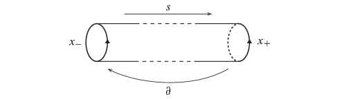
Figure 3.1: The differential in Floer cohomology goes from right to left.

Using once again Corollary 15, $\partial\circ\partial=0$ holds by standard arguments which appear in [AD14, Chapter 9]. The pair $(\operatorname{CF}^{\ast}(H),\partial)$ is thus a graded cochain complex that we call the Floer cochain complex of $H$.

3.1.2.  Filtered Floer cochain complex

The Hamiltonian action functional induces a filtration on the Floer cochain complex. For $a\in(\mathbb{R}\cup\left\{\pm\infty\right\})\setminus\operatorname{Spec}(H)$, we define

$$\operatorname{CF}_{<a}^{k}(H) =\bigoplus_{\begin{subarray}{c}x\in\mathcal{P}(H)\\ |x|=k,\ \mathcal{A}_{H}(x)<a\end{subarray}}\mathbb{Z}_{2}\expectationvalue{x}.$$

By definition, we have $\operatorname{CF}^{\ast}(H)=\operatorname{CF}_{<+\infty}^{\ast}(H)$. Lemma 16 assures that $\partial$ decreases the action. Thus, the restriction $\partial_{<a}:\operatorname{CF}_{<a}^{k}(H)\to\operatorname{CF}_{<a}^{k+1}(H)$ of the co-boundary operator is well defined and $(\operatorname{CF}_{<a}^{\ast}(H),\partial_{<a})$ is a sub-complex of $(\operatorname{CF}^{\ast}(H),\partial)$. Now, for $a,b\in(\mathbb{R}\cup\left\{\pm\infty\right\})\setminus\operatorname{Spec}(H)$ such that $a<b$, we can define the Floer cochain complex in the action window $(a,b)$ as the quotient

$$\operatorname{CF}_{(a,b)}^{\ast}(H) =\frac{\operatorname{CF}_{<b}^{\ast}(H)}{\operatorname{CF}_{<a}^{\ast}(H)},$$

on which we denote the projection of the co-boundary operator by

$$\partial_{(a,b)} :\operatorname{CF}_{(a,b)}^{k}(H)\to\operatorname{CF}_{(a,b)}^{k+1}(H).$$

Therefore, for $a,b,c\in(\mathbb{R}\cup\left\{\pm\infty\right\})\setminus\operatorname{Spec}(H)$ such that $a<b<c$, we have an inclusion and a projection

$$\iota_{a,a}^{b,c} :\operatorname{CF}_{(a,b)}^{\ast}(H)\to\operatorname{CF}_{(a,c)}^{\ast}(H),\quad\pi_{a,b}^{c,c}:\operatorname{CF}_{(a,c)}^{\ast}(H)\to\operatorname{CF}_{(b,c)}^{\ast}(H)$$

that produce the short exact sequence

For simplicity, we define $\iota^{<c}=\iota_{-\infty,-\infty}^{+\infty,c}$ and $\pi_{>b}=\pi_{-\infty,b}^{+\infty,+\infty}$.

3.1.3.  Filtered Floer cohomology

Let $a,b\in(\mathbb{R}\cup\left\{\pm\infty\right\})\setminus\operatorname{Spec}(H)$ such that $a<b$. The above filtered cochain complexes allow us to define the Floer cohomology group of $H$ in the action window $(a,b)$ as

$$\operatorname{HF}_{(a,b)}^{\ast}(H) =\frac{\ker\partial_{(a,b)}}{\operatorname{im}\partial_{(a,b)}}.$$

The full Floer cohomology group of $H$ is defined as $\operatorname{HF}^{\ast}(H)=\operatorname{HF}_{(-\infty,+\infty)}^{\ast}(H)$. For $a,b,c\in(\mathbb{R}\cup\left\{\pm\infty\right\})\setminus\operatorname{Spec}(H)$ such that $a<b<c$, the short exact sequence on the cochain level induces a long exact sequence in cohomology:

For $C^{2}$-small admissible Hamiltonians with small slope at infinity, the Floer cohomology recovers the standard cohomology of $D$.

Lemma 17 ([Rit13, Section 15.2]).

Let $H\in\mathcal{H}$ be a $C^{2}$-small Hamiltonian with $\tau_{H}<T_{0}$ for $T_{0}=\min\operatorname{Spec}(\partial D,\lambda)$. Then, we have an isomorphism

$$\Phi_{H}:\operatorname{H}^{\ast}(D)\to\operatorname{HF}^{\ast}(H).$$

Remark 18.

We can endow $\operatorname{HF}^{\ast}(H)$ with a ring structure [Rit13] where the product is given by the pair of pants product. The unit in $\operatorname{HF}^{\ast}(H)$, which we denote $1_{H}$, coincides with $\Phi_{H}(e_{D})$ where $e_{D}$ is the unit in $\operatorname{H}^{\ast}(D)$ .

3.1.4.  Compactly supported Hamiltonians

We can define the Floer cohomology of compactly supported Hamiltonians on Liouville domains by first extending to affine functions on the cylindrical portion of $\hat{D}$.

Definition 19.

Denote by $\mathcal{C}(D)$ the set of Hamiltonians with support in $S^{1}\times(D\setminus\partial D)$. Let $H\in\mathcal{C}(D)$ . For $\tau\in(0,\infty)\setminus\operatorname{Spec}(\partial D,\lambda)$, we define the $\tau$-extension $H^{\tau}\in\mathcal{H}_{1}$ of $H$ as follows. Fix $0<\varepsilon<1$,

• $H^{\tau}=H$ on $D$,

• $H^{\tau}=h_{\varepsilon}(r)$ on $\hat{D}\setminus D$,

• $h_{\varepsilon}(r)$ is convex for $r\in[1,1+\varepsilon]$ with $h_{\varepsilon}^{(k)}(1)=0$ for all $k\geq 0$, $h_{\varepsilon}^{\prime}(1+\varepsilon)=\tau$ and $h_{\varepsilon}^{(\ell)}(1+\varepsilon)=0$ for all $\ell>0$,

• $h_{\varepsilon}(r)=\tau(r-(1+\varepsilon/2))$ for $r\in[1+\varepsilon,+\infty)$.

The Floer cohomology of $H$ is defined as

$$\operatorname{HF}_{(a,b)}^{\ast}(H)=\operatorname{HF}_{(a,b)}^{\ast}(H^{\tau})$$

where $0<\tau<T_{0}$.

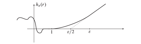
Figure 3.2: The $\tau$-extension of a compactly supported Hamiltonian.

Since we take a slope $\tau$ smaller than the minimum Reeb period to define $\operatorname{HF}_{(a,b)}^{\ast}(H)$, the above definition doesn’t depend on the choice of $\tau$ as we will see in Lemma 20 below.

3.1.5.  Continuation maps

Let $K\in\mathcal{H}_{r_{0}}$ and $F\in\mathcal{H}_{r_{0}^{\prime}}$ such that $F\leq K$. Consider a monotone homotopy $H_{\bullet}$ from $F$ to $K$. Then from Corollary 15 and Lemma 16 in the case of homotopies, we can apply the techniques shown in [AD14, Chapter 11] to show that, for $x_{-}\in\mathcal{P}(K)$ and $x_{+}\in\mathcal{P}(F)$ with $|x_{-}|=|x_{+}|$, $\mathcal{M}(x_{-},x_{+};H_{\bullet})$ is a smooth compact manifold of dimension zero. The continuation map $\Phi^{H_{\bullet}}:\operatorname{CF}^{k}(F)\to\operatorname{CF}^{k}(K)$ induced by $H_{s}$ on the cochain level is defined as

$$\Phi^{H_{\bullet}}(x_{+})=\sum_{|x_{-}|=k}\#_{2}\mathcal{M}(x_{-},x_{+};H_{\bullet})x_{-}$$

where $\#_{2}\mathcal{M}(x_{-},x_{+};H_{\bullet})$ is the count modulo 2 of components in $\mathcal{M}(x_{-},x_{+};H_{\bullet})$. The map

$$[\Phi^{H_{\bullet}}]:\operatorname{HF}^{\ast}(F)\to\operatorname{HF}^{\ast}(K)$$

is independent of the chosen monotone homotopy and we can denote it by $[\Phi^{K,F}]$. Consider the monotone homotopy

$$H_{s}=K+\beta(s)(F-K)$$

described in Section 2.2. We note that $\partial_{s}H_{s}\leq 0$ since $F\leq K$ and $\beta^{\prime}\geq 0$. Thus the action estimate given by Lemma 16 for homotopies yields

$$\mathcal{A}_{K}(x_{-})\leq\mathcal{A}_{H}(x_{+})+\sup_{\begin{subarray}{c}s\in[-S,S],\\ t\in S^{1},p\in D^{R}\end{subarray}}\partial_{s}H_{s}(t,p)\leq\mathcal{A}_{H}(x_{+})$$

for $x_{-}\in\mathcal{P}(K)$ and $x_{+}\in\mathcal{P}(F)$. Therefore, the continuation map decreases the action and hence induces maps

$$[\Phi_{(a,b)}^{K,F}]:\operatorname{HF}_{(a,b)}^{\ast}(F)\to\operatorname{HF}_{(a,b)}^{\ast}(K)$$

that commute with the inclusion and restriction maps as follows [Rit13, Section 8]:

(1)

Suppose we are given another Hamiltonian $H\geq K$, then we have the commutative diagram

As opposed to the closed case, for completion of Liouville domains, continuation maps do not necessarily yield isomorphisms. One case in which they do is when both Hamiltonians have the same slope.

Lemma 20 ([Web06, Section 2.1]).

Let $F,K\in\mathcal{H}$ and suppose $\tau_{F}$ and $\tau_{K}$ are both contained in an open interval that does not intersect $\operatorname{Spec}(\partial D,\alpha)$. Then,

• if $\tau_{F}=\tau_{K}$, $\Phi^{K,F}\circ\Phi^{F,K}=\mathrm{id}=\Phi^{F,K}\circ\Phi^{K,F}$ and thus $\operatorname{HF}^{\ast}(F)\cong\operatorname{HF}^{\ast}(K)$.

• if $\tau_{F}<\tau_{K}$, $[\Phi^{K,F}]:\operatorname{HF}^{\ast}(F)\to\operatorname{HF}^{\ast}(K)$ is an isomorphism.

Under these isomorphisms, $1_{F}$ and $1_{K}$ are identified.

In action windows, we have the following isomorphisms.

Lemma 21 ([Vit99, Proposition 1.1]).

Let $H_{\bullet}$ be a monotone homotopy between $H_{\pm}\in\mathcal{H}$ that is constant in the $s$-coordinate for $|s|>S>0$. Suppose $a_{s},b_{s}:\mathbb{R}\to\mathbb{R}$ are functions which are constant outside $[-S,S]$ and $a_{s},b_{s}\notin\operatorname{Spec}(H_{s})$ for all $s$. Then,

for $a_{\pm}=\lim_{s\to\pm\infty}a_{s}$ and $b_{\pm}=\lim_{s\to\pm\infty}b_{s}$.

3.2 Filtered Symplectic cohomology

Equip the set of admissible Hamiltonians $\mathcal{H}^{0}$ negative on $D$ with the partial order

$$H\preceq K\iff H(t,p)\leq K(t,p)\quad \forall(t,p)\in S^{1}\times\hat{D}.$$

Let $\{H_{i}\}_{i\in I}\subset\mathcal{H}^{0}$ be a cofinal sequence with respect to $\preceq$. We define the symplectic cohomology of $D$ as the direct limit

$$\operatorname{SH}_{(a,b)}^{\ast}(D)=\lim_{\begin{subarray}{c}\longrightarrow\\ H_{i}\end{subarray}}\operatorname{HF}_{(a,b)}^{\ast}(H_{i})$$

taken with respect to the continuation maps

$$[\Phi_{(a,b)}^{H_{j},H_{i}}] :\operatorname{HF}_{(a,b)}^{\ast}(H_{i})\to\operatorname{HF}_{(a,b)}^{\ast}(H_{j})$$

for $i<j$. We denote $\operatorname{SH}^{\ast}(D)=\operatorname{SH}_{(-\infty,+\infty)}^{\ast}(D)$. The long exact sequence on Floer cohomology carries through the direct limit and we also have a long exact sequence on symplectic cohomology

The Viterbo map.–Let $F\in\mathcal{H}$ and consider $H\in\mathcal{H}^{0}$ with $\tau_{H}=\tau_{F}$. Then, by Lemma 20, we have $\operatorname{HF}^{\ast}(F)\cong\operatorname{HF}^{\ast}(H)$ and there exist, by definition of symplectic cohomology, a map

$$j_{F}:\operatorname{HF}^{\ast}(F)\cong\operatorname{HF}^{\ast}(H)\to\operatorname{SH}^{\ast}(D)$$ (2)

sending each element of $\operatorname{HF}^{\ast}(H)$ to its equivalence class. Now, for $H\in\mathcal{H}^{0}$ with slope $\tau_{H}<T_{0}$ we can define, by Lemma 17 the map $v^{\ast}:\operatorname{H}^{\ast}(D)\to\operatorname{SH}^{\ast}(D)$ first introduced in [Vit99] by

This map induces a unit on symplectic cohomology. Recall that $1_{H}$ denotes the unit in $\operatorname{HF}^{\ast}(H)$ (see Remark 18).

Theorem 22 ([Rit13]).

The ring structure on $\operatorname{HF}^{\ast}(H)$ induces a ring structure on $\operatorname{SH}^{\ast}(D)$. The unit on $\operatorname{SH}^{\ast}(D)$ is given by the image of the unit $e_{D}\in\operatorname{H}^{\ast}(D)$ under the map $v^{\ast}$. Moreover,

$$v^{\ast}(e_{D})=[\iota_{-\infty,-\infty}^{\varepsilon,+\infty}](1_{H}).$$

4 Spectral invariants and spectral norm

4.1 Spectral invariants

Denote by $\operatorname{Ham}_{c}(D,\differential\lambda)$ the group of compactly supported Hamiltonian diffeomorphisms of $(D,\differential\lambda)$ and by $\operatorname{Symp}_{c}(D,\differential\lambda)$ the group of compactly supported symplectomorphisms of $(D,\differential\lambda)$. The Hofer norm of a compactly supported Hamiltonian $H\in\mathcal{C}(D)$ is defined as

$$\norm{H} =\int_{0}^{1}\left(\sup_{p\in D}H(t,p)-\inf_{p\in D}H(t,p)\right)\,\differential t.$$

Using the Hofer norm, we can define a bi-invariant metric [Hof90, LM95] on $\operatorname{Ham}_{c}(D,\differential\lambda)$ by

$$d_{H}(\varphi,\psi)=d_{H}(\varphi\psi^{-1},\mathrm{id}),\quad d_{H}(\varphi,\mathrm{id})=\inf\{\norm{H}\mid\varphi=\varphi_{H}\}.$$

Recall that $\mathcal{C}(D)$ forms a group under the multiplication

$$H\#K(t,p)= H(t,p)+K(t,(\varphi_{H}^{t})^{-1}(p))$$

with the inverse of some $H\in\mathcal{C}(D)$ given by $\overline{H}(t,p)=-H(t,\varphi_{H}^{t}(p))$.

From Lemma 17 and by definition of $\operatorname{HF}^{\ast}(H)$ for $H\in\mathcal{C}(D)$, we know that $\operatorname{HF}^{\ast}(H)\cong\operatorname{H}^{\ast}(D)$. For $\beta\in\operatorname{H}^{\ast}(D)$, we define, following [Sch00], the spectral invariant of $H$ relative to $\beta$ as

$$c(\beta,H)=\inf\{\ell\in\mathbb{R}\mid[\pi_{-\infty,\ell}^{+\infty,+\infty}]\circ[\iota_{-\infty,-\infty}^{\ell,+\infty}](\beta)=0\}.$$

The following proposition gathers all the properties of spectral invariants we need for the rest of the text. Proofs of these properties can be found in [FS07, Section 5].

Proposition 23.

Let $\beta,\eta\in H^{\ast}(D)$ and let $H,K\in\mathcal{C}(D)$. Then,

• [Continuity]

  $$\int_{0}^{1}\min_{x\in D}(K-H)\differential t\leq c(\beta,H)-c(\beta,K)\leq\int_{0}^{1}\max_{x\in D}(K-H)\differential t$$

• [Spectrality] $c(\beta,H)\in\operatorname{Spec}(H)$.

• [Triangle inequality] $c(\beta\smile\eta,H\#K)\leq c(\beta,H)+c(\eta,K).$

• [Monotonicity] If $H(t,x)\leq K(t,x)$ for all $(t,x)\in[0,1]\times D$, then $c(\beta,H)\geq c(\beta,K)$.

Remark 24.

The continuity property of Proposition 23 allows us to define spectral invariants of compactly supported continuous Hamiltonians $H\in C_{c}^{0}([0,1]\times D)$. They satisfy continuity, the triangle inequality and monotonicity.

4.1.1.  Additional properties of $c$

The following lemma assures us that spectral invariants are well defined on $\operatorname{Ham}_{c}(D,\differential\lambda)$. The proof relies on the spectrality and the triangle inequality.

Lemma 25.

Let $H,K\in\mathcal{C}(D)$ such that $\varphi_{H}=\varphi_{K}$ and let $\beta\in\operatorname{H}^{\ast}(D)$. Then,

$$c(\beta,H)=c(\beta,K)$$

Proof.

We have $\varphi_{H\#\overline{K}}=\varphi_{0}=\mathrm{id}$ and in that case $\operatorname{Spec}(H\#\overline{K})=\{0\}$. Now, by spectrality of spectral invariants, $c(\beta,H\#\overline{K})=0$. Thus, the triangle inequality yields

$$c(\beta,H)=c(\beta,H\#\overline{K}\#K)\leq c(\beta,H\#\overline{K})+c(\beta,K)=c(\beta,K).$$

Repeating the same argument with $K\#\overline{H}$ instead of $H\#\overline{K}$, we obtain $c(\beta,K)\leq c(\beta,H)$ which concludes the proof. ∎

The spectral invariant with respect to the cohomological unit admits an implicit definition which depends on the spectral invariants with respect to all other cohomology classes in $\operatorname{H}^{\ast}(D)$. This follows directly from the triangle inequality.

Lemma 26.

Let $H\in\mathcal{C}(D)$. Then,

$$c(1,H)=\max_{\beta\in\operatorname{H}^{\ast}(D)}c(\beta,H).$$

Proof.

Let $\beta\in H^{\ast}(D)$. By definition of the unit and the concatenation of Hamiltonians, we have

$$c(\beta,H)=c(\beta\smile 1,H)=c(\beta\smile 1,0\#H).$$

Then, since $c(\beta,0)=0$, the triangle inequality guaranties that

$$c(\beta,H)=c(\beta\smile 1,0\#H)\leq c(\beta,0)+c(1,H)=c(1,H).$$

The choice of $\beta$ being arbitrary, this concludes the proof. ∎

4.1.2.  The symplectic contraction principle

We conclude this section by recalling the symplectic contraction technique introduced by Polterovich [Pol14, Section 5.4]. This principle allows one to describe the effect of the Liouville flow $\{\psi_{Y}^{\log r}\}_{0<r<1}$ on spectral invariants.

First, we need to describe how the Liouville flow acts on the symplectic form $\omega$ of $D$ and on compactly supported Hamiltonians on $D$. Since $L_{Y}\omega=\omega$, we have that the Liouville flow contracts the symplectic form :

$$\left(\psi_{Y}^{\log r}\right)^{\ast}\omega=r\omega$$

Now, consider a Hamiltonian $H\in\mathcal{C}(D)$ supported in $U\subset D$. For fixed $0<r<1$ define the Hamiltonian

$$H_{r}(t,x)=\begin{cases}rH\left(t,\left(\psi_{Y}^{\log r}\right)^{-1}(x)\right)&\text{if }x\in\psi_{Y}^{\log r}(U),\\ 0&\text{if }x\notin\psi_{Y}^{\log r}(U).\end{cases}$$ (3)

It then follows from the two previous equations that $\operatorname{Spec}(H_{r})=r\operatorname{Spec}(H)$. This allows one to prove

Lemma 27 ([Pol14]).

Suppose $H\in\mathcal{C}(D)$ and let $H_{r}\in\mathcal{C}(D)$ be as in Equation 3. Then,

$$c(1,H_{r})=rc(1,H).$$

4.2 Spectral norm

We define the spectral norm $\gamma(H)$ of $H\in\mathcal{C}(D)$ as

$$\gamma(H)=c(1,H)+c(1,\overline{H}).$$

For $\varphi\in\operatorname{Ham}_{c}(D,\differential\lambda)$ such that $\varphi=\varphi_{H}$, define

$$\gamma(\varphi)=\gamma(H)$$

In virtue of Lemma 25, this is well defined.

From [FS07, Section 7], we have the following theorem which justifies calling $\gamma$ a norm.

Theorem 28.

Let $\varphi,\psi\in\operatorname{Ham}_{c}(D,\differential\lambda)$ and let $\chi\in\operatorname{Symp}_{c}(D,\differential\lambda)$. Then,

• [Non-degeneracy] $\gamma(\mathrm{id})=0$ and $\gamma(\varphi)>0$ if $\gamma\neq\mathrm{id}$,

• [Triangle inequality] $\gamma(\varphi\psi)\leq\gamma(\varphi)+\gamma(\psi)$,

• [Symplectic invariance] $\gamma(\chi\circ\varphi\circ\chi^{-1})=\gamma(\varphi)$,

• [Symmetry] $\gamma(\varphi)=\gamma(\varphi^{-1})$,

• [Hofer bound] $\gamma(\varphi)\leq d_{H}(\varphi,\mathrm{id})$.

5 Cohomological barricades on Liouville domains

In [GT] Ganor and Tanny introduced a particular perturbation of Hamiltonians compactly supported inside contact incompressible boundary domains (CIB) of closed aspherical symplectic manifolds. For instance, if $U\subset M$ is an incompressible open set which is a Liouville domain, then $U$ is a CIB. In Floer homology, the aforementioned Hamiltonian perturbation, which is called a barricade, prohibits the existence of Floer trajectories exiting and entering the CIB. We consider barricades in the particular case of Liouville domains and adapt them to Floer cohomology.

Definition 29.

Let $r_{0}>1$ and $0<\varepsilon<r_{0}-1$. Define $B_{r_{0},\varepsilon}=D^{r_{0}-\varepsilon}\setminus D$ where, for $\rho>0$, $D^{\rho}=\Psi_{Y}^{\log\rho}(D)$. Suppose $(F_{\bullet},J)$ is a pair of a monotone homotopy $F_{\bullet}$ from $F_{+}$ to $F_{-}$ and an admissible almost complex structure $J$. We say that $(F_{\bullet},J)$ admits a barricade on $B_{r_{0},\varepsilon}$ if for every $x_{\pm}\in\mathcal{\mathcal{P}}(F_{\pm})$ and every Floer trajectory $u:\mathbb{R}\times S^{1}\to\hat{D}$ connecting $x_{\pm}$, we have, for $D_{\text{b}}:=D^{r_{0}-\varepsilon}=D\cup B_{r_{0},\varepsilon}$

1. If $x_{-}\in D$, then $\operatorname{im}(u)\subset D$,

2. If $x_{+}\in D_{b}$, then $\operatorname{im}(u)\subset D_{\text{b}}$.

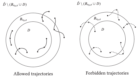
Figure 5.1: Floer cylinders in a barricade.

Remark 30.

In the language of [GT], a barricade on $B_{r_{0},\varepsilon}$ as described above would be called a barricade in $D^{r_{0}-\varepsilon}$ around $D$.

5.1 How to construct barricades

To construct barricades, we consider the following class of pairs.

Definition 31.

Let $r_{0}>1$, $\sigma\in(0,+\infty)\setminus\operatorname{Spec}(\partial D,\lambda)$ and $0<\varepsilon<r_{0}-1$. The pair $(F_{\bullet},J)$ admits a cylindrical bump of slope $\sigma$ on $B_{r_{0},\varepsilon}$ if

• $F=0$ on $\partial B_{r_{0},\varepsilon}\times S^{1}\times\mathbb{R}$,

• $JY=R_{\alpha}$, for $Y$ the Liouville vector field on $D$, on a neighborhood of $\partial B_{r_{0},\varepsilon}$, i.e. $J$ is cylindrical near $\partial B_{r_{0},\varepsilon}=\partial D\sqcup(\{r_{0}-\varepsilon\}\times\partial D)$.

• $\nabla_{J}F=\sigma Y$ near $(\{1\}\times\partial D)\times S^{1}\times\mathbb{R}$ and $\nabla_{J}F=-\sigma Y$ near $(\{r_{0}-\varepsilon\}\times\partial D)\times S^{1}\times\mathbb{R}$. Here, $\nabla_{J}$ denotes the gradient induced by the metric $g_{J}$.

• All 1-periodic orbits of $F_{\pm}$ contained in $B_{r_{0},\varepsilon}$ are critical points with values in the interval $(-\sigma,\sigma)$. (In particular, $\sigma<T_{0}$.)

A cohomological adaptation of Lemma 3.3 in [GT] yields the following action estimates for pairs with cylindrical bumps.

Lemma 32.

Suppose that $(F,J)$ admits a cylindrical bump of slope $\sigma$ on $B_{r_{0},\varepsilon}$. For every finite energy solution $u$ connecting $x_{\pm}\in\mathcal{P}(F_{\pm})$, then

• $x_{-}\subset D$ and $x_{+}\subset\hat{D}\setminus D$ $\implies$ $\mathcal{A}_{F_{+}}(x_{+})>\sigma$,

• $x_{+}\subset D$ and $x_{-}\subset\hat{D}\setminus D$ $\implies$ $\mathcal{A}_{F_{-}}(x_{-})>\sigma$,

• $x_{-}\subset D_{\text{b}}$ and $x_{+}\subset\hat{D}\setminus D_{\text{b}}$ $\implies$ $\mathcal{A}_{F_{+}}(x_{+})<-\sigma$,

• $x_{+}\subset D_{\text{b}}$ and $x_{-}\subset\hat{D}\setminus D_{\text{b}}$ $\implies$ $\mathcal{A}_{F_{-}}(x_{-})<-\sigma$.

Lemma 32 and the maximum principle are all we need to prove that every pair with a cylindrical bump admits a barricade. More precisely, we have the

Proposition 33.

Let $(F,J)$ be a pair with a cylindrical bump of slope $\sigma$ on $B_{r_{0},\varepsilon}$. Then, $(F,J)$ admits a barricade on $B_{r_{0},\varepsilon}$.

Proof.

Suppose $u:\mathbb{R}\times S^{1}\to\hat{D}$ is a Floer trajectory between $x_{\pm}\in\mathcal{P}(F_{\pm})$. We only need to study the case where $x_{-}\in D$ and the case where $x_{+}\in D_{\text{b}}$.

Suppose that $x_{-}\in D$. We first establish that $x_{+}$ must lie inside $D$. Indeed, if $x_{+}\in\hat{D}\setminus D$, Lemma 32 assures us that $\mathcal{A}_{F_{+}}(x_{+})>\sigma$ which contradicts the fact that orbits on $\hat{D}\setminus D$ must have action in the interval $(-\sigma,\sigma)$ by the construction of the cylindrical bump. Therefore, $x_{+}\in D$ as desired. Now, since $x_{\pm}\in D$, the maximum principle guarantees that $\operatorname{im}u\subset D$.

To finish the proof, we look at the case where $x_{+}\in D_{\text{b}}$. Similarly to the previous case, we prove that $x_{-}$ also lies inside $D_{\text{b}}$. If $x_{-}\in\hat{D}\setminus D_{\text{b}}$, Lemma 32 imposes $\mathcal{A}_{F_{-}}(x_{-})<-\sigma$, which is again impossible by construction of the cylindrical bump. Therefore, $x_{-}\in D_{\text{b}}$ and the maximum principle implies $\operatorname{im}u\subset D_{\text{b}}$. ∎

Given a pair $(F,J)$ and $\sigma>0$ small, we can add to $F$ a $\mathcal{C}^{\infty}$-small radial bump function $\chi$ with support inside $B_{r_{0},\varepsilon}$ such that $(F+\chi,J)$ has a cylindrical bump of slope $\sigma$ on $B_{r_{0},\varepsilon}$. By Proposition 33, the perturbed pair will also admit a barricade on $B_{r_{0},\varepsilon}$. A second perturbation of the Hamiltonian term at its ends, under which the barricade survives, allows us to achieve Floer regularity for the pair. This procedure is carried out carefully in [GT, section 9] and yields the following.

Theorem 34 ([GT]).

Let $F_{\bullet}$ be a monotone homotopy. Then, there exists a $\mathcal{{C}}^{\infty}$-small perturbation $f_{\bullet}$ of $F_{\bullet}$ and an almost complex structure $J$ such that the pairs $(f_{\bullet},J)$ and $(f_{\pm},J)$ are Floer-regular and have a barricade on $B_{r_{0},\varepsilon}$.

5.2 Decomposition of the Floer cochain complex

Let us investigate what structure barricades impose on the Floer co-chain complex. Let $H\in\mathcal{H}_{r_{0}}$ and suppose the pair $(H,J)$ admits a barricade on $B_{r_{0},\varepsilon}$. For an open subset $U\subset\hat{D}$, denote by $\operatorname{C}^{\ast}(U,H)$ the set of $1$-periodic orbits of $H$ in $U$. By definition of the differential $\partial$ on Floer cohomology, $\operatorname{C}^{\ast}(D_{\text{b}},H)$ is closed under $\partial$ and it therefore forms a sub-complex of $\operatorname{CF}^{\ast}(H)$. Moreover, for $D_{\text{c}}=\hat{D}\setminus D_{\text{b}}$, we also have that

$$\operatorname{C}^{\ast}(D_{\text{c}},H) =\frac{\operatorname{CF}^{\ast}(H)}{\operatorname{C}^{\ast}(D_{\text{b}},H)}$$

is a well defined cochain complex.

5.2.1.  Continuation maps

Let $(F_{\bullet},J)$ be a pair that admits a barricade on $B_{r_{0},\varepsilon}$ where $F_{\bullet}$ is a monotone homotopy from $F_{+}$ to $F_{-}$. Then, since the continuation map $\Phi_{F_{\bullet}}:\operatorname{CF}^{\ast}(F_{+})\to\operatorname{CF}^{\ast}(F_{-})$ counts Floer trajectories of $F$ connecting 1-periodic orbits of $F_{+}$ to 1-periodic orbits of $F_{-}$, it restricts, due to the barricade, to a chain map

$$\Phi^{\text{b}}_{F}:\operatorname{C}^{\ast}(D_{\text{b}},F_{+})\to\operatorname{C}^{\ast}(D_{\text{b}},F_{-})$$ .

Moreover, in virtue of Lemma 36 below, $\Phi_{F}$ projects to a chain map

$$\Phi^{\text{c}}_{F} :\operatorname{C}^{\ast}(D_{\text{c}},F_{+})\to\operatorname{C}^{\ast}(D_{\text{c}},F_{-})$$

such that the following diagram commutes

for $\pi_{+}^{\text{b}}$ and $\pi_{-}^{\text{b}}$ the canonical projections.

5.2.2.  Chain homotopies

For $F_{\pm}\in\mathcal{H}_{r_{0}}$ , consider the linear homotopy

$$F_{s} =F_{-}+\beta(s)(F_{+}-F_{-})$$

where $\beta:\mathbb{R}\to[0,1]$ is a smooth function such that $\beta(s)=0$ for $s\leq-1$, $\beta(s)=1$ for $s\geq 1$ and $\beta^{\prime}(s)>0$ for all $s\in(-1,1)$. Denote by $\overline{F}_{\bullet}$ the inverse homotopy defined by $\overline{F}_{s}=F_{-s}$. For $\rho>1$ large, we define the concatenation $F\#\overline{F}_{\bullet}$ as

$$(F\#\overline{F})_{s} =\begin{cases}F_{s+\rho}&\text{for }s\leq 0\\ \overline{F}_{s-\rho}&\text{for }s\geq 0\end{cases}.$$

Using the definition of $F_{\bullet}$ and $\overline{F}_{\bullet}$, we can simply write

$$(F\#\overline{F})_{s} =F_{-}+\beta_{\rho}(s)(F_{+}-F_{-})$$

for $\beta_{\rho}(s)=\beta(-|s|+\rho)$. The homotopy $F\#\overline{F}_{\bullet}$ generates the composition of continuation homomorphisms $\Phi_{F}\circ\Phi_{\overline{F}}:\operatorname{CF}^{\ast}(F_{-})\to\operatorname{CF}^{\ast}(F_{-})$ which is chain homotopic to the identity on $\operatorname{CF}^{\ast}(F_{-})$,

$$\Phi_{F_{\bullet}}\circ\Phi_{\overline{F}_{\bullet}}-\mathrm{id}_{-} =\partial_{-}\circ\Psi_{-}-\Psi_{-}\circ\partial_{-}$$

for $\Psi_{-}:\operatorname{CF}^{\ast}(F_{-})\to\operatorname{CF}^{\ast-1}(F_{-})$ and $\partial_{-}$ the differential on $\operatorname{CF}^{\ast}(F_{-})$. The chain homotopy $\Psi_{-}$ is built by counting Floer solutions of the homotopy $\left\{\Gamma^{\kappa}\right\}_{\kappa\in[0,1]}$ between $F\#\overline{F}_{\bullet}$ and the constant homotopy $F_{-}$ which is defined by

$$\Gamma_{s}^{\kappa}=F_{-}+\kappa\beta_{\rho}(s)(F_{+}-F_{-}).$$

For $x\in\mathcal{P}(F_{-})$ and $y\in\mathcal{P}(F_{+})$, define

$$\mathcal{M}^{\Gamma}(x,y)=\left\{(\kappa,u)\mid\kappa\in[0,1],\ u\in\mathcal{M}(x,y;\Gamma_{\bullet}^{k})\right\}.$$

We can perturb $\Gamma$ with a $C^{\infty}$-small function in order to make it regular [AD14, Chapter 11]. Now, if $F_{-}$ and $F_{+}$ admit barricades on $B_{r_{0},\varepsilon}$, solutions to the parametric Floer equation for $\Gamma^{\kappa}$ also admit barricades on $B_{r_{0},\varepsilon}$. The same holds with its regular perturbation.

Lemma 35.

Let $F_{-},F_{+}\in\mathcal{H}_{r_{0}}$ and suppose they both admit a barricade on $B_{r_{0},\varepsilon}$. Then, for any $C^{\infty}$-small perturbation $\Gamma^{\prime}$ of $\Gamma$ which satisfies $\mathcal{P}(F^{\prime}_{\pm})=\mathcal{P}(F_{\pm})$, Floer trajectories in $\mathcal{M}^{\Gamma^{\kappa}}$ follow the rules of the barricade on $B_{r_{0},\varepsilon}$.

Proof.

The proof follows the same ideas as the proof of Proposition 9.21 in [GT]. By Gromov compactness, any sequence $(\kappa_{n},u_{n})\in\mathcal{M}^{\Gamma}(x_{-},y_{+})$ of solutions to the parametric Floer equation converges, up to taking a subsequence, to a broken trajectory $(\kappa,\bar{v})$ where $\bar{v}=(v_{1},\ldots,v_{k},w,v_{1}^{\prime},\ldots,v_{\ell}^{\prime})$ connects two orbits $x_{\pm}\in\mathcal{P}(F_{\pm})$ . The fact that $F_{\pm}$ both admit a barricade on $B_{r_{0},\varepsilon}$ assures us that

• $x_{-}\in D$ $\implies$ $\bar{v}\subset D$

• $x_{+}\in D$ $\implies$ $\bar{v}\subset D_{\text{b}}$.

Now, consider a sequence of regular homotopies $\left\{\Gamma_{n}\right\}_{n}$ with ends $\lim_{s\to\pm\infty}\Gamma_{s,n}=F_{n\pm}$ converging to $\Gamma$ such that $\mathcal{P}(F_{n\pm})=\mathcal{P}(F_{\pm})$ for all $n$. Then, the above two implications regarding broken trajectories imply that every trajectory $(\kappa_{n},u_{n}^{\prime})\in\mathcal{M}^{\Gamma}(x_{-},x_{+})$, for $x_{\pm}\in\mathcal{P}(F_{\pm})$, obeys to the rules of the barricade. ∎

Thus, $\Psi_{-}$ restricts to a map $\Psi_{-}^{b}:\operatorname{C}^{\ast}(D_{\text{b}},F_{-})\to\operatorname{C}^{\ast-1}(D_{\text{b}},F_{-})$ and by Lemma 37 below, we can define its projection $\Psi_{-}^{c}:\operatorname{C}^{\ast}(D_{\text{c}},F_{-})\to\operatorname{C}^{\ast-1}(D_{\text{c}},F_{-})$.

Technical lemmas.– When adapting computations from homology to cohomology, we often have to rely on quotient complexes instead of sub-complexes. Here are a few simple results from homological algebra which will be useful in that regard. Let $(A,d_{A})$ and $(C,d_{C})$ be cochain complexes and let $B\subset A$ and $D\subset C$ be sub-complexes.

Lemma 36.

Suppose $f:(A,B)\to(C,D)$ is a chain map. Then, there exists a unique chain map $\bar{f}:A/B\to C/D$ such that the following diagram commutes

for $\pi_{B}$ and $\pi_{D}$ the canonical projections. It follows that, on cohomology, we have the following commutative diagram.

Proof.

Define, for all $x\in A$,

$$\bar{f}(\pi_{B}(x)) =\pi_{D}(f(x)).$$

We first need to show that $\bar{f}$ is well defined. Suppose $x^{\prime}=x+b$ for $x\in A$ and $b\in B$. Then, since $f$ restricts to a map from $B$ to $D$, there exists $d\in D$ such that $f(b)=d$ and we have

$$\bar{f}(\pi_{B}(x^{\prime})) =\pi_{D}(f(x+b))=\pi_{D}(f(x)+d)=\pi_{D}(f(x)).$$

Thus, $\bar{f}$ is well defined.

To prove uniqueness, we simply use the definition of $\bar{f}$. Suppose we have another map $\bar{g}:A/B\to C/D$ which makes the above diagram commute as well. Then, for all $x\in A$,

$$\bar{f}(\pi_{B}(x))-\bar{g}(\pi_{B}(x)) =\pi_{D}(f(x))-\pi_{D}(f(x))=0.$$

∎

Lemma 37.

Suppose $f:(A,B)\to(C,D)$ and $g:(C,D)\to(A,B)$ are chain maps such that $f\circ g$ is chain homotopic to the identity

$$f\circ g-\mathrm{id}_{C} =d_{C}\circ\psi-\psi\circ d_{C}$$

where the chain homotopy is a map $\psi:(C,D)\to(C,D)$. Then, $\bar{f}\circ\bar{g}:C/D\to C/D$ is also chain homotopic to the identity.

Proof.

Since the chain homotopy $\psi:(C,D)\to(C,D)$ is a chain map of pairs, Lemma 36 allows us to define its projection $\bar{\psi}:C/D\to C/D$. Thus, for all $y\in C$,

$$\bar{f}\circ\bar{g}(\pi_{D}(y))-\mathrm{id}_{C/D}(\pi_{D}(y)) =\bar{f}\circ\pi_{B}(g(y))-\pi_{D}(\mathrm{id}_{C}(y))$$

$$=\pi_{D}(f\circ g(y))-\pi_{D}(\mathrm{id}_{C}(y))$$

$$=\pi_{D}((d_{C}\circ\psi-\psi\circ d_{C})(y))$$

$$=(d_{C/D}\circ\pi_{D}\circ\psi-\pi_{D}\circ\psi\circ d_{C})(y)$$

$$=d_{C/D}\circ\bar{\psi}(\pi_{D}(y))-\bar{\psi}\circ d_{C/D}(\pi_{D}(y))$$

which proves that $\bar{f}\circ\bar{g}$ is chain homotopic to the identity on $C/D$ since any $z\in C/D$ is of the form $z=\pi_{D}(y)$. ∎

6 Proofs of main results

6.1 Proof of Theorem A1

Fix $A\in(0,\infty)\setminus\operatorname{Spec}(\partial D,\lambda)$. The idea of the proof is to construct a special admissible Hamiltonian for which $c(1,\cdot)$ is bounded from below by $A-\varepsilon$ for $\varepsilon$ a small constant which depends on $A$. This construction is inspired by [CFO10, Proposition 2.5]. Then, we use the fact that $c(1,\cdot)\geq 0$ to conclude.

6.1.1.  Construction of the Hamiltonian

For any $\delta\in(0,1)$ and $\sigma\in(0,T_{0})$, we define the Hamiltonian $H_{\delta,A}\in\mathcal{H}_{r_{0}}$ as follows:

• $H_{\delta,A}$ is the constant function $A(\delta-1)$ on $D^{\delta}$,

• $H_{\delta,A}(r,x)=A(r-1)$ on $D\setminus D^{\delta}$,

• $H_{\delta,A}(r,x)=0$ on $D^{r_{0}}\setminus D$

• $H_{\delta,A}(r,x)=\sigma(r-r_{0})$ on $\hat{D}\setminus D^{r_{0}}$.

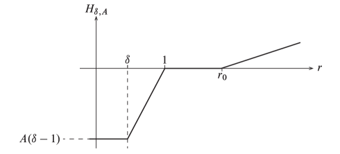
Figure 6.1: Radial portion of the Hamiltonian $H_{\delta,A}$.

We add a small perturbation to $H_{\delta,A}$ so that it lies in $\mathcal{H}_{r_{0}}$. Denote by $h_{\delta,A}$ the restriction of $H_{\delta,A}$ to $\hat{D}\setminus D$. If $\gamma$ is a 1-periodic orbit of $h_{\delta,A}$ inside the level set $\left\{r\right\}\times\partial D,$ its action can be written as

$$\mathcal{A}_{H_{\delta,A}}(\gamma)=\mathcal{A}_{H_{\delta,A}}(r)=rh^{\prime}_{\delta,A}(r)-h_{\delta,A}(r).$$

The 1-periodic orbits of $H_{\delta,A}$ can be classified in three different categories. Recall that $\eta_{A}$ denotes the distance between $A$ and $\operatorname{Spec}(\partial D,\alpha)$.

• Critical points in $D^{\delta}$ with action close to $r_{\text{I}}=(1-\delta)A$

• Non-constant 1-periodic orbits near $\left\{\delta\right\}\times\partial D$ with action in a small neighborhood of the interval

  $$I_{\text{II}}=[\delta T_{0}+(1-\delta)A,\,A-\delta\eta_{A}].$$

• Non-constant 1-periodic orbits near $\left\{1\right\}\times\partial D$ with action in a small neighborhood of the interval

  $$I_{\text{III}}=[T_{0},\,A-\eta_{A}].$$

• Critical points in $D^{r_{0}}\setminus D$ with action close to $r_{\text{IV}}=0$.

Note that there are no non-constant 1-periodic orbits near $\left\{r_{0}\right\}\times\partial D$, since the slope of the Hamiltonian there ranges from $0$ to $\sigma$ which is less than $T_{0}$ by assumption.

We now want to construct a Floer complex $\operatorname{C}_{\text{{I,II}}}^{\ast}$ which will contain the orbits of type (I) and (II) and another complex $\operatorname{C}_{\text{{III,IV}}}^{\ast}$ containing orbits of type (III) and $(\text{IV})$. To that end, pick $0<\delta<1$ small enough so that $\delta A<\eta_{A}$. Now choose $\varepsilon>0$ such that

$$\delta A<\varepsilon<\eta_{A}.$$

Then, we have the following inequalities :

$$r_{\text{IV}}<I_{\text{III}}<A-\varepsilon<r_{\text{I}}<I{}_{\text{II}}.$$

Figure 6.2: Distances that separate the action windows under consideration.

As shown in Figure 6.2, $r_{\text{\text{I}}}$, $I_{\text{II}}$, $I_{\text{III}}$ and $r_{\text{IV}}$ are all separated by distances which depend only on $T_{0}$, $A$, $\eta_{A}$, $\delta$ and $\varepsilon$. Thus, we can choose the perturbation we add to $H_{\delta,A}$ to be small enough so that, in terms of action, we have

$$(\text{IV})<(\text{{III}})<A-\varepsilon<(\text{{I}})<(\text{{II}}).$$

Therefore, since the Floer differential decreases the action, we can define the Floer co-chain complexes as

$$\operatorname{C}_{\text{{III,IV}}}^{\ast}=\operatorname{CF}_{<A-\varepsilon}^{\ast}(H_{\delta,A}),\quad\operatorname{C}_{\text{{I,II}}}^{\ast}=\frac{{\operatorname{CF}^{\ast}(H_{\delta,A})}}{\operatorname{C}_{\text{{III,IV}}}^{\ast}}=\operatorname{CF}_{(A-\varepsilon,\infty)}^{\ast}(H_{\delta,A})$$

and they yield the Floer cohomology groups

$$\operatorname{H}^{\ast}(\operatorname{C}_{\text{III,IV}}^{\ast})=\operatorname{HF}_{(-\infty,A-\varepsilon)}^{\ast}(H_{\delta,A}),\quad\operatorname{H}^{\ast}(\operatorname{C}_{\text{I,II}}^{\ast})=\operatorname{HF}_{(A-\varepsilon,\infty)}^{\ast}(H_{\delta,A}).$$

A quick look at the action windows under consideration informs us that the above complexes fit into the following short exact sequence

which in turn yields an exact triangle in cohomology

6.1.2.  Factoring a map to $\operatorname{SH}^{\ast}(D)$

We now build maps $\Psi$ and $\Psi_{\text{{I,II}}}$ such that the diagram

(4)

commutes. We need to construct $\Psi$ so that it coincides with the map $j_{H_{\delta,A}}:\operatorname{HF}^{\ast}(H_{\delta,A})\to\operatorname{SH}^{\ast}(D)$ (see Equation 2). In virtue of Theorem 22, this assures us that $\Psi$ is a map of unital algebras.

First, we construct $\Psi_{\text{{I,II}}}$ in three steps.

STEP 1. $[\Phi_{1}]:\operatorname{H}^{\ast}(\operatorname{C}_{\text{{I,II}}}^{\ast})\cong\operatorname{HF}_{(\delta A-\varepsilon,\infty)}^{\ast}(H_{\delta,A}+A(1-\delta)).$ This isomorphism follows from a simple shift of $A(1-\delta)$ in the Hamiltonian term which translates to a shift of $A(\delta-1)$ in action (see Figure 6.3). In what follows, we denote $\hat{H}_{\delta,A}:=H_{\delta,A}+A(1-\delta)$.

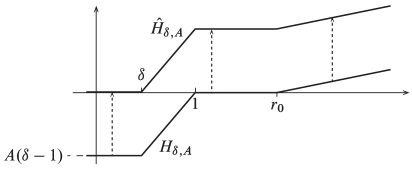
Figure 6.3: Homotopy from $H_{\delta,A}$ to $\hat{H}_{\delta,A}.$

For the next steps, we need to define another special family of Hamiltonians. Given $r_{1}\in(0,+\infty)$ and $\tau\in(0,\infty)\setminus\operatorname{Spec}(\partial D,\lambda)$, define the Hamiltonian $K_{r_{1},\tau}$ as follows (see Figure 6.4).

• $K_{r_{1},\tau}$ is a $C^{2}$-small perturbation of the constant zero function on $D^{r_{1}}$,

• $K_{r_{1},\tau}(x,r)=\tau(r-r_{1})$ on $\hat{D}\setminus D^{r_{1}}$.

The 1-periodic orbits of a suitable perturbation of $K_{r_{1},\tau}$ fall in two categories.

• Critical points in $D^{r_{1}}$ with action near zero,

• Non-constant 1-periodic orbits near $\left\{r_{1}\right\}\times\partial D$ with action in a small neighborhood of the interval

  $$[r_{1}T_{0},r_{1}\tau-r_{1}\eta_{\tau}].$$

By the same argument used for $H_{\delta,A}$, the action windows $(\text{I}^{\prime})$ and $(\text{II}^{\prime})$ are separated if we choose a small enough perturbation.

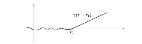
Figure 6.4: Radial portion of the Hamiltonian $K_{r_{0},\tau}$.

STEP 2. $[\Phi_{2}]:\operatorname{HF}_{(\delta A-\varepsilon,\infty)}^{\ast}(\hat{H}_{\delta,A})\cong\operatorname{HF}_{(\delta A-\varepsilon,\infty)}^{\ast}(K_{\delta,A}).$ Consider the homotopy

$$F_{s}=(1-\beta(s))K_{\delta,A}+\beta(s)\hat{H}_{\delta,A},$$

where $\beta:\mathbb{R}\to[0,1]$ is a smooth function such that $\beta(s)=0$ for $s\leq-1$, $\beta(s)=1$ for $s\geq 1$ and $\beta^{\prime}(s)>0$ for all $s\in(-1,1)$ (see Figure 6.5). Denote by

the continuation map generated by $F_{\bullet}$.

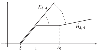
Figure 6.5: Homotopy from $\hat{H}_{\delta,A}$ to $K_{\delta,A}$.

The new orbits created by $\Phi_{F_{\bullet}}$ near $\left\{1\right\}\times\partial D$ will have action in the interval

$$[T_{0}+A(\delta-1),\delta A-\eta_{A}]$$

which, since $\varepsilon<\eta_{A}$ by assumption, is disjoint from $(\delta A-\varepsilon,\infty)$. Hence these new orbits will all appear out of the action window under consideration. Thus, Lemma 21 assures us that $[\Phi_{2}]$ is an isomorphism.

STEP 3. Recall from Equation 2, that we have a natural map

$$\leavevmode\hbox to177.43pt{\vbox to19.06pt{\text{[drawing]}}}. {j_{K_{\delta},A}:\operatorname{HF}^{\ast}_{(\delta A-\varepsilon,+\infty)}(K_{\delta,A})} {\operatorname{SH}^{\ast}_{(\delta A-\varepsilon,+\infty)}(D)\cong\operatorname{SH}^{\ast}(D)} {j_{K_{\delta},A}:\operatorname{HF}^{\ast}_{(\delta A-\varepsilon,+\infty)}(K_{\delta,A})} {\operatorname{SH}^{\ast}_{(\delta A-\varepsilon,+\infty)}(D)\cong\operatorname{SH}^{\ast}(D)}$$

The isomorphism to $\operatorname{SH}^{\ast}(D)$ follows from the fact that, by construction, $\delta A-\varepsilon<0$.

We define $\Psi_{\text{{I,II}}}:\operatorname{H}^{\ast}(\operatorname{C}_{\text{I,II}}^{\ast})\to\operatorname{SH}_{(\delta A-\varepsilon,+\infty)}^{\ast}(D)$ to the composition

$$\Psi_{\text{I,II}}=j_{K_{\delta,A}}\circ[\Phi_{2}]\circ[\Phi_{1}].$$

The morphism $\Psi$ is built in a similar fashion. We define it as the composition of the maps

Here, the isomorphism $[\Phi_{1}^{\prime}]$ follows from the fact that both $H_{\delta,A}$ and $\hat{H}_{\delta,A}$ have the same slope at infinity. We defined $[\Phi_{2}^{\prime}]$ to be the composition of the continuation map $[\Phi^{K_{\delta,A}\hat{H}_{\delta,A}}]$ and the projection $[\pi_{-\infty,\delta A-\varepsilon}^{+\infty+\infty}]:\operatorname{HF}^{\ast}(K_{\delta,A})\to\operatorname{HF}_{(\delta A-\varepsilon+\infty)}^{\ast}(K_{\delta,A})$ which is an isomorphism. The last map is given, just as in STEP 3, by $j_{K_{\delta,A}}:\operatorname{HF}^{\ast}(K_{\delta,A})\to\operatorname{SH}^{\ast}(D)$ . By construction, we therefore have

$$\Psi=j_{K_{\delta,A}}\circ[\Phi_{2}^{\prime}]\circ[\Phi_{1}^{\prime}]=j_{K_{\delta,A}}\circ[\pi_{-\infty,\delta A-\varepsilon}^{+\infty,+\infty}]\circ[\Phi_{K_{\delta,A}\hat{H}_{\delta,A}}]\circ[\Phi_{1}^{\prime}]=j_{H_{\delta,A}}$$

as desired.

Now, we need to prove that Diagram (4) commutes. Writing the maps $\Psi$ and $\Psi_{\text{I,II}}$ explicitly, we have the following diagram:

(5)

The top square in Diagram 5 commutes because, since $\hat{H}_{\delta,A}\geq H_{\delta,A}$, there exists a continuation map from $\operatorname{HF}^{\ast}(H_{\delta,A})$ to $\operatorname{HF}_{(\delta A-\varepsilon,+\infty)}^{\ast}(\hat{H}_{\delta,A})$. Now, since the projection $[\pi_{-\infty,\delta A-\varepsilon}^{+\infty,+\infty}]$ commutes with continuation maps (see Diagram 1), the bottom square in Diagram 5 also commutes. Therefore, we can conclude that Diagram (4) commutes.

6.1.3.  Spectral invariant and spectral norm of $H_{\delta,A}$

Recall that, by definition,

$$c(1,H_{\delta,A})=\inf\{c\in\mathbb{R}\mid[\pi_{-\infty,\ell}^{+\infty,+\infty}]\circ[\iota_{-\infty,-\infty}^{\ell,+\infty}](1)=0\}$$

Since $\Psi$ is a morphism of unital algebras, the commutative diagram (4) assures us that $[\pi_{-\infty,A-\varepsilon}^{+\infty,+\infty}](1_{H_{\delta,A}})\neq 0.$ Thus, from the exact triangle in cohomology induced by $[\iota_{-\infty,-\infty}^{A-\varepsilon,+\infty}]$ and $[\pi_{-\infty,A-\varepsilon}^{+\infty,+\infty}]$, we have $1\notin\operatorname{im}[\iota_{-\infty,-\infty}^{A-\varepsilon,+\infty}]$ and therefore,

$$c(1,H_{\delta,A})\geq A-\varepsilon.$$

Now, we turn our attention to the spectral norm $\gamma(H_{\delta,A})$. We know from Lemma B that $c(1,H_{\delta,A}),c(1,\overline{{H}}_{\delta,A})\geq 0$. It thus follows from the previous inequality that

$$\gamma(H_{\delta,A})=c(1,H_{\delta,A})+c(1,\overline{{H}}_{\delta,A})\geq A-\varepsilon$$

as desired. This completes the proof.

6.2 Proof of Lemma B

We give a proof of Lemma B which relies on the decomposition of the Floer complex induced by the barricade. We expect that Lemma B could also be proven using Poincaré duality and Lemma 4.1 of [GT].

Let $H\in\mathcal{H}_{r_{0}}$ with slope $0<\tau_{H}<T_{0}$. Consider a linear homotopy $F_{\bullet}$ from $F_{+}=K_{r_{0},\tau}$ for $0<\tau<T_{0}$(see Figure 6.4) to $F_{-}=H$ . There exists a small perturbation $f_{\bullet}$ of $F_{\bullet}$ and an almost complex structure $J$ such that the pairs $(f_{\bullet},J)$ and $(f_{\pm},J)$ admit a barricade on $B_{r_{0},\varepsilon}$ for $\varepsilon>0$ small enough. Fix $\delta>0$. The construction allows us to choose $J$ time independent and $f$ such that

$$-\delta\leq\int_{0}^{1}\min_{x\in\hat{D}\setminus(r_{0},+\infty)\times\partial D}(f_{-}-H)\differential t\leq\delta.$$

We may assume further that $f_{+}$ has a local minimum point $p\in D_{\text{c}}$, since $f_{+}$ is $C^{2}$-small there. It follows from Lemma 17 that $1_{f_{+}}=[p]\in\operatorname{HF}^{\ast}(f_{+})$ is the image of the unit $e_{D}\in\operatorname{H}^{\ast}(D)$ under the isomorphism $\Phi_{f_{+}}:\operatorname{H}^{\ast}(D)\to\operatorname{HF}^{\ast}(f_{+})$. Moreover, Lemma 20 assures us that the isomorphism $[\Phi_{f_{\bullet}}]:\operatorname{HF}^{\ast}(f_{+})\to\operatorname{HF}^{\ast}(f_{-})$ induced by the continuation morphism $\Phi_{f_{\bullet}}:\operatorname{CF}^{\ast}(f_{+})\to\operatorname{CF}^{\ast}(f_{-})$ preserves the unit. To summarize, we have

$$\Phi_{f_{+}}(e_{D})=[p]=1_{f_{+}}\quad\text{{and}$\quad$}[\Phi_{f_{\bullet}}(p)]=[\Phi_{f_{\bullet}}](1_{f_{+}})=1_{f_{-}}.$$

By the continuity of spectral invariants, we know that

$$c(1,H)-c(1,f_{-})\geq\int_{0}^{1}\min_{x\in\hat{D}\setminus(r_{0},+\infty)\times\partial D}(f_{-}-H)\differential t$$ .

Therefore, by our choice of $f_{-}$, we have $c(1,H)\geq-\delta+c(1,f_{-}).$ To complete the proof, it suffices to show that $c(1,f_{-})\geq-k\delta$ for $k$>0 independent of $f_{-}$. However, the definition of spectral invariants guarantees the existence of $q\in\operatorname{CF}^{\ast}(f_{-})$ cohomologous to $1$ for which $c(1,f_{-})\geq\mathcal{A}_{f_{-}}(q)-\delta$. We thus only need to prove that $\mathcal{A}_{f_{-}}(q)\geq-\delta.$

Recall that, by the barricade construction, $\operatorname{C}^{\ast}(D_{\text{b}},f_{-})$ forms a sub-complex of $\operatorname{CF}^{\ast}(f_{-})$. Moreover,

$$\operatorname{C}^{\ast}(D_{\text{c}},f_{-})=\frac{\operatorname{CF}^{\ast}(f_{-})}{\operatorname{C}^{\ast}(D_{\text{b}},f_{-})}$$

where we denote the projection by $\pi_{-}^{\text{c}}:\operatorname{CF}^{\ast}(f_{-})\to\operatorname{C}^{\ast}(D_{\text{c}},f_{-})$. This allows us to write

$$\Phi_{f_{\bullet}}(p) =p_{\text{b}}+p_{\text{c}}\ \text{and}\>q=p_{\text{b}}+p_{\text{c}}+\partial(r_{\text{b}}+r_{\text{c}})$$

for $p_{\text{b}},r_{\text{b}}\in\operatorname{C}^{\ast}(D_{\text{b}},f_{-})$ and $p_{\text{c}},r_{\text{c}}\in\operatorname{C}^{\ast}(D_{\text{c}},f_{-})$. Again, from the barricade construction, we have

$$\partial(r_{\text{b}}+r_{0})=r_{\text{bb}}+r_{\text{cb}}+r_{\text{cc}}$$

where $r_{\text{bb}},r_{\text{cb}}\in\operatorname{C}^{\ast}(D_{\text{b}},f_{-})$ and $r_{\text{cc}}\in\operatorname{C}^{\ast}(D_{\text{c}},f_{-})$. Notice that since $f_{-}$ is $C^{2}$-small on $D_{\text{c}}$, $\mathcal{A}_{f_{-}}(p_{\text{c}}+r_{\text{cc}})\geq-\delta.$ Thus, if $p_{\text{c}}+r_{\text{cc}}\neq 0$, we have

$$\mathcal{A}_{f_{-}}(q)=\mathcal{A}_{f_{-}}(p_{\text{b}}+p_{\text{c}}+r_{\text{bb}}+r_{\text{cb}}+r_{\text{cc}})\geq\mathcal{A}_{f_{-}}(p_{\text{c}}+r_{\text{cc}})\geq-\delta.$$

We now prove that $[p_{\text{c}}]\in\operatorname{H}^{\ast}(D_{\text{c}},f_{-})$ is not zero which is equivalent to showing that $p_{\text{c}}+r_{\text{cc}}\neq 0$. Denote by $\Phi_{\bar{f}_{\bullet}}:\operatorname{CF}^{\ast}(f_{-})\to\operatorname{CF}^{\ast}(f_{+})$ the continuation map generated by the inverse homotopy $\overline{f}_{s}=f_{-s}$. We know that both $\Phi_{\bar{f}_{\bullet}}\circ\Phi_{f_{\bullet}}$ and $\Phi_{f_{\bullet}}\circ\Phi_{\bar{f}_{\bullet}}$ are chain homotopic to the identity :

$$\Phi_{\bar{f}_{\bullet}}\circ\Phi_{f_{\bullet}}-\mathrm{id}_{+} =\partial_{+}\circ\Psi_{+}-\Psi_{+}\circ\partial_{+}$$

$$\Phi_{f_{\bullet}}\circ\Phi_{\bar{f}_{\bullet}}-\mathrm{id}_{-} =\partial_{-}\circ\Psi_{-}-\Psi_{-}\circ\partial_{-}$$

for the differentials $\partial_{\pm}:\operatorname{CF}^{\ast}(f_{\pm})\to\operatorname{CF}^{\ast+1}(f_{\pm})$ and chain homotopies $\Psi_{\pm}:\operatorname{CF}^{\ast}(f_{\pm})\to\operatorname{CF}^{\ast-1}(f_{\pm})$. (In fact, for our purpose here, we only need the first homotopy relation.) Since $\Psi_{\pm}$ also obey the rules of the barricade by Lemma 35, the composition of the projections $\Phi^{\text{c}}_{f_{\bullet}}:\operatorname{C}^{\ast}(D_{\text{c}},f_{+})\to\operatorname{C}^{\ast}(D_{\text{c}},f_{-})$ and $\Phi^{\text{c}}_{\bar{f}_{\bullet}}:\operatorname{C}^{\ast}(D_{\text{c}},f_{-})\to\operatorname{C}^{\ast}(D_{\text{c}},f_{+})$ are chain homotopic to the identity on $\operatorname{C}^{\ast}(D_{\text{c}},f_{+})$ by Lemma 37. Therefore, on cohomology, the morphism

$$[\Phi^{\text{c}}_{\bar{f}_{\bullet}}\circ\Phi_{f_{\bullet}}^{c}] :\operatorname{H}^{\ast}(D_{\text{c}},f_{+})\to\operatorname{H}^{\ast}(D_{\text{c}},f_{+})$$

is given by the identity and since $[p]\neq 0$,

$$[p_{\text{c}}]=[\Phi^{\text{c}}_{f_{\bullet}}(p)]=[\Phi^{\text{c}}_{f_{\bullet}}]([p])\neq 0.$$

This concludes the proof.

6.3 Proof of Lemma C

Let $0<\delta<1$ be small enough so that

$$\delta A<\delta A+\delta\eta_{A}<\eta_{A}.$$

Then, following the proof of Theorem A1, we have that

$$c(1,H_{\delta,A})\geq A-\delta(A+\eta_{A}).$$

Notice that $H_{\delta,A}$ converges uniformly as $\delta\to 0$ to the continuous function $H_{0,A}$ (see Figure 6.6). Then, by continuity of spectral invariants and the previous equation, we have

$$c(1,H_{0,A})=\lim_{\delta\to 0}c(1,H_{\delta,A})\geq\lim_{\delta\to 0}\left(A-\delta(A+\eta_{A})\right)=A.$$

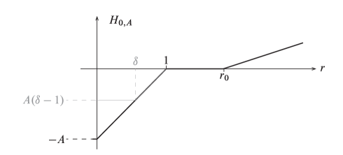
Figure 6.6: The continuous Hamiltonian $H_{0,A}$.

Moreover, since $H_{0,A}\geq-A$, continuity of spectral invariants yields

$$c(1,H_{0,A})\leq\max_{x\in D}-H_{0,A}=A$$

which allows us to conclude that $c(1,H_{0,A})=A.$

First, we prove the Lemma for Hamiltonians which are constant on an open neighborhood of the Skeleton of $D$. Consider an autonomous Hamiltonian $H\in\mathcal{C}(D)$ such that $H\big{|}_{V}=-A$ and $-A\leq H\leq 0$ for an open neighborhood $V$ of $\operatorname{Sk}(D)$ and a constant $A>0$. The last condition on $H$ allows us to use continuity of spectral invariance to conclude that

$$c(1,H)\leq A.$$ (6)

All we need to do now is prove that $A$ bounds $c(1,H)$ from below.

Define $F\in\mathcal{C}(D)$ to be the continuous autonomous Hamiltonian that agrees with $H_{0,A/r^{\prime}}$ on $D$ for some $0<r^{\prime}<1$. Since $H\big{|}_{V}=-A$ , we can choose $r^{\prime}$ so that the $r^{\prime}$-contraction $F_{r^{\prime}}$ of $F$ under the Liouville flow (see Equation 3 and Figure 6.7), has support in $V$ and $-A\leq F_{r^{\prime}}\leq 0$. Therefore,

$$F_{r^{\prime}}(x)\geq H(x),\quad\forall x\in D.$$ (7)

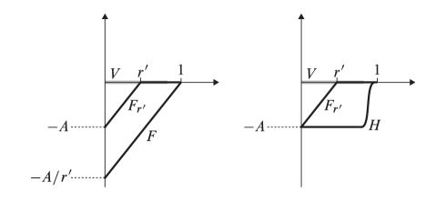
Figure 6.7: The Hamiltonians $F$, $F_{r^{\prime}}$ and $H$.

From the contraction principle stated in Lemma 27 and the computation of $c(1,H_{0,A})$ above, we have

$$c(1,F_{r^{\prime}})=r^{\prime}c(1,F)=r^{\prime}c(1,H_{0,A/r})=A.$$

This computation and Equation 7 yield, by virtue of the monoticity of spectral invariants, the lower bound $A=c(1,F_{r^{\prime}})\leq c(1,H)$ as desired. In conjunction with Equation 6, we conclude that $c(1,H)=A$.

Now, we prove the Lemma in general. Suppose $H\big{|}_{\operatorname{Sk}(D)}=-A$ and $-A\leq H\leq 0$. For any $\varepsilon\in(0,1)$, there exists a compactly supported Hamiltonian $H_{\varepsilon}$ such that $H_{\varepsilon}\big{|}_{V_{\varepsilon}}=-A$ for an open neighborhood $V_{\varepsilon}$ of $\operatorname{Sk}(D)$ and $H_{\varepsilon}\leq H$ everywhere. Indeed, define $H_{\varepsilon}$ as follows : $H_{\varepsilon}\big{|}_{\operatorname{Sk}(D)}=-A$,

$$H_{\varepsilon}\big{|}_{D^{\varepsilon}\setminus\operatorname{Sk}(D)} =\beta_{\varepsilon}(r)H+(1-\beta_{\varepsilon}(r))(-A)$$

where $\beta_{\varepsilon}:(0,1)\to\mathbb{R}$ is such that

• $\beta_{\varepsilon}\big{|}_{(0,\varepsilon]}\equiv 0$,

• $\beta^{\prime}_{\varepsilon}\big{|}_{(\varepsilon,2\varepsilon/3)}>0,$

• $\beta_{\varepsilon}\big{|}_{(2\varepsilon/3,1)}\equiv 1.$

Then, $H_{\varepsilon}$ satisfies the required conditions and converges uniformly to $H$ as $\varepsilon\to 0$. We have $c(1,H_{\varepsilon})$ by the previous computation and by continuity of spectral invariants, we can conclude that

$$c(1,H)=c(1,H_{\varepsilon})=A.$$

This completes the proof.

6.4 Proof of Theorem A2

Let $H\in\mathcal{C}(D)$ be an autonomous Hamiltonian such that $H\big{|}_{V}=-1$ and $-1\leq H\leq 0$ everywhere for an open neighborhood $V$ of $\operatorname{Sk}(D)$.

Define $\iota:\mathbb{R}\to\operatorname{Ham}_{c}(D)$ as

$$\iota(s)=\varphi_{sH}$$ ,

where $\varphi_{sH}\in\operatorname{Ham}_{c}(D)$ is the time-one map associated to $sH$. We claim that $\iota$ is the desired embedding.

We first bound $d_{\gamma}(\iota(s),\iota(s^{\prime}))$ from above. If $F\in\mathcal{C}(D)$, then $\gamma(\varphi_{F})\leq\norm{F}$. Moreover, since $H$ is autonomous, $sH\#\overline{{s^{\prime}H}}=(s-s^{\prime})H$. Therefore,

$$d_{\gamma}(\iota(s),\iota(s^{\prime})) =\gamma(\iota(s)\iota(s^{\prime})^{-1})\leq\norm{(s-s^{\prime})H}=\absolutevalue{s-s^{\prime}}.$$

Now, we bound $d_{\gamma}(\iota(s),\iota(s^{\prime}))$ from below. Since $d_{\gamma}$ is symmetric, we can assume that $s\geq s^{\prime}$. Then, by Lemma B and Lemma C, we have

$$d_{\gamma}(\iota(s),\iota(s^{\prime}))\geq c(1,(s-s^{\prime})H)=s-s^{\prime}$$ ,

which completes the proof.

References

- [AD14] M. Audin and M. Damian. Morse theory and Floer homology. Universitext. Springer, London; EDP Sciences, Les Ulis, 2014. Translated from the 2010 French original by Reinie Erné.
- [BHS21] L. Buhovsky, V. Humilière, and S. Seyfaddini. The action spectrum and symplectic topology. Math. Ann., 380(1-2):293–316, 2021.
- [BK] G. Benedetti and J. Kang. Relative Hofer-Zehnder capacity and positive symplectic homology. J. Fixed Point Theory Appl., to appear. Available at arXiv:2010.15462, 2020.
- [CE12] K. Cieliebak and Y. Eliashberg. From Stein to Weinstein and back, volume 59 of American Mathematical Society Colloquium Publications. American Mathematical Society, Providence, RI, 2012. Symplectic geometry of affine complex manifolds.
- [CFH95] K. Cieliebak, A. Floer, and H. Hofer. Symplectic homology. II. A general construction. Math. Z., 218(1):103–122, 1995.
- [CFHW96] K. Cieliebak, A. Floer, H. Hofer, and K. Wysocki. Applications of symplectic homology. II. Stability of the action spectrum. Math. Z., 223(1):27–45, 1996.
- [CFO10] K. Cieliebak, U. Frauenfelder, and A. Oancea. Rabinowitz Floer homology and symplectic homology. Ann. Sci. Éc. Norm. Supér. (4), 43(6):957–1015, 2010.
- [EP03] M. Entov and L. Polterovich. Calabi quasimorphism and quantum homology. Int. Math. Res. Not., (30):1635–1676, 2003.
- [FH94] A. Floer and H. Hofer. Symplectic homology. I. Open sets in . Math. Z., 215(1):37–88, 1994.
- [FS07] U. Frauenfelder and F. Schlenk. Hamiltonian dynamics on convex symplectic manifolds. Israel J. Math., 159:1–56, 2007.
- [Gir91] E. Giroux. Convexité en topologie de contact. Comment. Math. Helv., 66(4):637–677, 1991.
- [Gir17] E. Giroux. Remarks on Donaldson’s symplectic submanifolds. Pure Appl. Math. Q., 13(3):369–388, 2017.
- [GT] Y. Ganor and S. Tanny. Floer theory of disjointly supported Hamiltonians on symplectically aspherical manifolds. Algebr. Geom. Topol, to appear. Available at arXiv:2005.11096, 2021.
- [Hof90] H. Hofer. On the topological properties of symplectic maps. Proc. Roy. Soc. Edinburgh Sect. A, 115(1-2):25–38, 1990.
- [Kawa] Yusuke Kawamoto. Homogeneous quasimorphisms, -topology and lagrangian intersection. Comment. Math. Helv., to appear. Available at arXiv:2006.07844, 2019.
- [Kawb] Yusuke Kawamoto. On -continuity of the spectral norm for symplectically non-aspherical manifolds. Int. Math. Res. Not. IMRN, to appear. Available at arXiv:1905.07809, 2020.
- [KS21] A. Kislev and E. Shelukhin. Bounds on spectral norms and barcodes. Geom. Topol., 25(7):3257–3350, 2021.
- [LM95] F. Lalonde and D. McDuff. The geometry of symplectic energy. Ann. of Math. (2), 141(2):349–371, 1995.
- [LR10] F. Le Roux. Six questions, a proposition and two pictures on Hofer distance for Hamiltonian diffeomorphisms on surfaces. In Symplectic topology and measure preserving dynamical systems, volume 512 of Contemp. Math., pages 33–40. Amer. Math. Soc., Providence, RI, 2010.
- [LZ18] R. Leclercq and F. Zapolsky. Spectral invariants for monotone lagrangians. Journal of Topology and Analysis, 10(03):627–700, 2018.
- [MVZ12] A. Monzner, N. Vichery, and F. Zapolsky. Partial quasimorphisms and quasistates on cotangent bundles, and symplectic homogenization. J. Mod. Dyn., 6(2):205–249, 2012.
- [Oh05] Y.-G. Oh. Construction of spectral invariants of Hamiltonian paths on closed symplectic manifolds. In The breadth of symplectic and Poisson geometry, volume 232 of Progr. Math., pages 525–570. Birkhäuser Boston, Boston, MA, 2005.
- [Oh15] Y.-G. Oh. Symplectic topology and Floer homology. Vol. 2, volume 29 of New Mathematical Monographs. Cambridge University Press, Cambridge, 2015. Floer homology and its applications.
- [Pol01] L. Polterovich. The geometry of the group of symplectic diffeomorphisms. Lectures in Mathematics ETH Zürich. Birkhäuser Verlag, Basel, 2001.
- [Pol14] L. Polterovich. Symplectic geometry of quantum noise. Comm. Math. Phys., 327(2):481–519, 2014.
- [Rit13] A. F. Ritter. Topological quantum field theory structure on symplectic cohomology. J. Topol., 6(2):391–489, 2013.
- [Sch00] M. Schwarz. On the action spectrum for closed symplectically aspherical manifolds. Pacific J. Math., 193(2):419–461, 2000.
- [Sei08] P. Seidel. A biased view of symplectic cohomology. In Current developments in mathematics, 2006, pages 211–253. Int. Press, Somerville, MA, 2008.
- [SZ92] D. Salamon and E. Zehnder. Morse theory for periodic solutions of Hamiltonian systems and the Maslov index. Comm. Pure Appl. Math., 45(10):1303–1360, 1992.
- [Ush13] M. Usher. Hofer’s metrics and boundary depth. Ann. Sci. Éc. Norm. Supér. (4), 46(1):57–128 (2013), 2013.
- [Vit92] C. Viterbo. Symplectic topology as the geometry of generating functions. Math. Ann., 292(4):685–710, 1992.
- [Vit99] C. Viterbo. Functors and computations in Floer homology with applications. I. Geom. Funct. Anal., 9(5):985–1033, 1999.
- [Web06] J. Weber. Noncontractible periodic orbits in cotangent bundles and Floer homology. Duke Math. J., 133(3):527–568, 2006.
- [Wei79] A. Weinstein. On the hypotheses of Rabinowitz’ periodic orbit theorems. Journal of Differential Equations, 33(3):353–358, 1979.