Deep Stochastic Optimization in Finance

Abstract

This paper outlines, and through stylized examples evaluates a novel and highly effective computational technique in quantitative finance. Empirical Risk Minimization (ERM) and neural networks are key to this approach. Powerful open source optimization libraries allow for efficient implementations of this algorithm making it viable in high-dimensional structures. The free-boundary problems related to American and Bermudan options showcase both the power and the potential difficulties that specific applications may face. The impact of the size of the training data is studied in a simplified Merton type problem. The classical option hedging problem exemplifies the need of market generators or large number of simulations.

Key words: ERM, Neural Networks, Hedging, American Options.
Mathematics Subject Classification: 91G60, 49N35, 65C05.

1 Introduction

Readily available and effective optimization libraries such as Tensorflow or Pytorch now make previously intractable regression type of algorithms over hypothesis spaces with large number of parameters computationally feasible. In the context of stochastic optimal control and nonlinear parabolic partial differential equations which have such representations, these exciting advances allow for a highly efficient computational method. This algorithm, which we call deep empirical risk minimization, proposed by E & Han [21] and E, Jentzen & Han [22], uses artificial neural networks to approximate the feedback actions which are then trained by empirical risk minimization. As stochastic optimal control is the unifying umbrella for almost all hedging, portfolio or risk management problems, and many models in financial economics, this method is also highly relevant for quantitative finance.

Although artificial neural networks as approximate controls are widely used in optimal control and reinforcement learning [6], deep empirical risk minimization simulates directly the system dynamics and does not necessarily use dynamic programming. It aims to construct optimal actions and values offline by using the assumed dynamics and the rewards structure, and often uses market generators to simulate large training data sets. This key difference between reinforcement learning and the proposed algorithm ushers in essential changes to their implementations and analysis as well.

Our goal is to outline this demonstrably effective methodology, assess its strengths and potential shortcomings, and also showcase its power through representative examples from finance. As verified in its numerous applications, deep empirical risk minimization is algorithmically quite flexible and handles well a large class of high-dimensional models, even non-Markovian ones, and adapts to complex structures with ease. To further illustrate and evaluate these properties, we also study three classical problems of finance with this approach. Additional examples from nonlinear partial differential equations and stochastic optimal control are given in the recent survey articles of Fecamp, Mikael & Warin [15] and Germain, Pham & Warin [19]. They also provide an exhaustive literature review.

Our first class of examples is the American and Bermudan options. The analysis of these instruments offer many-faceted complex experiments through which one appreciates the potentials and the challenges. In a series of papers, Becker et al., [4, 5] bring forth a complete analysis with computable theoretical upper bounds through its known convex dual. They also obtain inspiring computational results in high dimensional problems such as Bermudan max-call options with $500$ underlyings. Akin to deep empirical risk minimization is the seminal regression on Monte-Carlo methods that were developed for the American options by Longstaff & Schwartz [29] and Tsitsiklis & van Roy [38]. Many of their refinements, as delineated in the recent article of Ludkovski [30], make them not only textbook topics but also standard industrial tools. Still, the deep empirical risk minimization approach to optimal stopping has some advantages over them, including its effortless ability to incorporate market details and frictions, and to operate in high-dimensions as caused by state enlargements needed for path-dependent claims. An example of the latter is the American options with rough volatility models as studied by Chevalier at. al. [11]. They require infinite-dimensional spaces and their numerical analysis is given in Bayer et al. [3]. Other similar examples can be found in [4, 5].

For interpretability of our results, we base the stopping decisions on a surface separating the ‘continuation’ and ‘stopping’ regions, and approximate directly this boundary - often called the free boundary - by an artificial neural network. Similarly for the same reason, Ciocan & Mis̆ic [12] compute the free boundary directly, by using tree based methods. An additional benefit of this geometric approach to American options is to construct a tool that can also be effectively used for financial problems with discontinuous decisions such as regime-switching or transaction costs, as well as non-financial applications. Indeed, the computation of the free-boundary is an interesting problem independent of applications to finance. Recently, deep Galerkin method [37] is used to compute the free boundary arising in the classical Stephan problem of melting ice [39].

Our numerical results, reported in the subsections 4.5 and 4.6 below, show that natural problem specific modifications enable the general approach to yield excellent results comparable to the ones achieved in [4, 5]. The free boundaries that we compute for the two-dimensional max-call options also compare to the results by Broadie & Detemple [8] and by Detemple [14]. An important step in our approach is to replace the stopping rule given by the sharp interface by a relaxed stopping rule given by a fuzzy boundary as described in the subsection 4.4. Further analysis and the results of our free-boundary methodology are given in our future manuscript [32].

Our second example of classical quadratic hedging [36] is undoubtedly one of the most compelling benchmark for any computational technique in quantitative finance. Thus, the evaluation of the deep empirical risk minimization algorithm on this problem, imparts valuable insights. Readily, Bühler et al., [9, 10] use this approach for multidimensional Heston type models, delivering convincing evidence for the flexibility and the scope of the algorithm, particularly in high-dimensions. Huré et al., [25] and Bachouch et al., [2] also obtain equally remarkable results for the stochastic optimal control using empirical minimization as well as other hybrid algorithms partially based on dynamic programming. Extensive numerical experimentations are also carried out by Fecamp et. al. [15] in an incomplete market that models the electricity markets containing a non-tradable volume risk [40]. Ruf & Wang [33] apply this approach to market data of S&P 500 and Euro Stoxx 50 options. In all these applications, variants of the quadratic hedging error is used as the loss function.

To highlight the essential features, we focus on a simple frictionless market with Heston dynamics, and consider a vanilla Call option with quadratic loss. In this setting, we analyze both the pure hedging problem by fixing the price at a level lower than its known value and also the pricing and hedging problem by training for the price as well. By the well-known results of Schweizer [35, 36] and Föllmer & Schweizer [18], we know that the minimizer of the analytical problem in the continuous time is equal to the price obtained by Heston [23] as the discounted expected value under the risk neutral measure with the chosen market risk of volatility risk. Our numerical computations verify these results as well.

As the final example, we report the results of an accompanying paper of the first two authors [31] for a stylized Merton type problem. With simulated data, the numerical results once again showcase the flexibility and the scope of the algorithm, in this problem as well. We also observe that in data-poor environments, the artificial neural networks have an amazing capability to over-learn the data causing poor generalization. This is one of the key results of [31] which was also observed in [28]. Despite this potential, as demonstrated by our experiments, continual data simulation can overcome this difficulty swiftly.

In this paper, we only discuss the properties of the algorithms that are variants of the deep empirical risk minimization. The use of artificial neural networks or statistical machine learning is of course not limited to this approach. Indeed, starting from [26] and especially recently, artificial neural networks have been extensively employed in quantitative finance. In particular, kernel methods are applied to portfolio valuation in [7], and to the density estimation in [16]. Gonon et. al. [20] use the methodology to study an equilibrium problem in a market with frictions. For further results and more information, we refer to the recent survey of Ruff & Wang [34] and the references therein.

The paper is organized as follows. The next section formulates the control problem abstractly covering many important financial applications. The description of the algorithm follows. Section 4 is about the American and Bermudan options. The quadratic hedging problem is the topic of Section 5. Finally, the numerical examples related to the simple Merton problem are discussed in Section (6).

Acknowledgements. Research of the second and the third authors was partially supported by the National Science Foundation grant DMS 2106462.

2 Abstract problem

Following the formulation of [31], we start with a ${\mathcal{Z}}\subset\mathbb{R}^{d}$ valued stochastic process $Z$ on a probability space $\Omega$. This process drives the dynamics of the problem, and in all financial examples that we consider it is the related to the stock returns. For that reason, in the sequel, we refer to $Z$ as the returns process, although they may be logarithmic returns in some cases. Investment or hedging decisions are made at $N$ uniformly spaced discrete time points labeled by $k=0,1,\ldots,N$ and let

$${\mathcal{T}}:=\{0,1,\ldots,N-1\},\qquad\widehat{{\mathcal{T}}}:=\{0,1,\ldots,N\}.$$

We use the notation $Z=(Z_{1},\ldots,Z_{N})$ and set $Z_{0}=0$. We further let $\mathbb{F}=({\mathcal{F}}_{t})_{t=0,\ldots,N}$ be the filtration generated by the process $Z$. The $\mathbb{F}$-adapted controlled state process $X$ takes values in another Euclidean space ${\mathcal{X}}$ and it may include all or some components of the uncontrolled returns process $Z$.

In the financial examples, the state includes the marked-to-market value of the portfolio and maybe other relevant quantities. In a path-dependent structure, we would be forced to include not only the current value of the portfolio and the return, but also some past values as well (theoretically, we need to keep all past values but in practice one stops at a finite point). In illiquid markets, the portfolio composition is also included into the state and even the order-book might be considered. We assume that the state is appropriately chosen so that the relevant decisions are feedback functions of the state alone and we optimize over feedback decisions or controls. Thus, even if the original problem is low dimensional but non-Markov, one is forced to expand the state resulting in a high-dimensional problem.

We denote the set of possible actions or decisions by ${\mathcal{A}}$. While the main decision variable is the portfolio composition, several other quantities such as the speed of the change of the portfolio could be included. Then, a feedback decision is a continuous function

$$\pi:{\mathcal{T}}\times{\mathcal{X}}\mapsto{\mathcal{A}}.$$

We let ${\mathcal{C}}$ be the set of all such functions. Given $\pi\in{\mathcal{C}}$, the time evolution of the state vector is then completely described as a function of the returns process $Z$. Hence, all optimization problems that we consider have the following form,

$$\text{minimize}\quad v(\pi):=\mathbb{E}\left[\,\ell(\pi,Z)\,\right],\qquad\text{over all}\ \pi\in{\mathcal{C}},$$

where $\ell$ is a nonlinear function. We refer the reader to [31] for a detailed derivation of the above formulation and several examples. Although the cost function $\ell$ could be quite complex to express analytically, it can be easily evaluated by simply mimicking the dynamics of the financial market. Hence, computationally they are straight-forward to compute and all details of the markets can be easily coded into it.

The goal is to compute the optimal feedback decision, $\pi^{*}$, and the optimal value $v^{*}$,

$$\pi^{*}\in\text{argmin}_{\pi\in{\mathcal{C}}}\,v(\pi),\qquad v^{*}:=\inf_{\pi\in{\mathcal{C}}}\,v(\pi)\ =\ v(\pi^{*}).$$

When the underlying dynamics is Markovian and the cost functional has an additive structure, the above formulation of optimization over feedback controls is equivalent to the standard formulation which considers the larger class of all adapted processes, sometimes called open loop controls [17]. However, even without this equivalence, the minimization over the smaller class of feedback controls is a consistent and a well-defined problem, and due to their tractability, feedback controls are widely used. In this manuscript, we implicitly assume that the problem is well chosen and the goal is to construct the best feedback control.

3 The algorithm

In this section, we describe the deep empirical minimization algorithm proposed by Weinan E, Jiequn Han, and Arnulf Jentzen in [21, 22].

A batch $B:=\{Z^{1},\ldots,Z^{m}\}$, with a size of $m$, is an i.i.d. realization of the returns process $Z$, where $Z^{i}=(Z^{i}_{1},\ldots,Z^{i}_{N})$ for each $i$. We set

$$L(\pi,B):=\frac{1}{m}\,\sum_{i=1}^{m}\,\ell(\pi,Z^{i}),$$

and consider a set of artificial neural networks parametrized by,

$${\mathcal{N}}=\left\{\,\Phi(\cdot;\theta):{\mathcal{T}}\times{\mathcal{X}}\mapsto{\mathcal{A}}\ \ :\ \theta\in\Theta\ \right\}\,\subset\,{\mathcal{C}}.$$

Instead of searching for a minimizer in ${\mathcal{C}}$, we look for a computable solution in the smaller set ${\mathcal{N}}$. That is, numerically we approximate the following quantities:

$$\theta^{*} :=\theta^{*}_{\mathcal{N}}\in\text{argmin}_{\theta\in\Theta}\,v(\Phi(\cdot;\theta)),$$

$$v_{{\mathcal{N}}} :=\inf_{\theta\in\Theta}\,v(\Phi(\cdot;\theta))=v(\Phi(\cdot;\theta^{*})).$$

The classical universal approximation result for artificial neural networks [13, 24] imply, under some natural structural assumptions on the function $\ell$, that $v_{{\mathcal{N}}}$ approximates $v^{*}$ as the networks gets larger as proved in [31](Theorem 5). This also implies that the performance of the trained feedback control $\Phi(\cdot;\theta^{*})$ is almost optimal.

The pseudocode of the algorithm to compute $\theta^{*}$ and $v^{*}$ is the following,

• Initialize $\theta\in\Theta$;

• Optimize by stochastic gradient descent: for $n=0,1,\ldots$:

  • Generate a batch $B:=\{Z^{1},\ldots,Z^{m}\}$,

  • Compute the derivative $d:=\nabla_{\theta}\,L(\Phi(\cdot;\theta),B)$;

  • Update $\theta\,\leftarrow\,\theta-\kappa d$.

• Stop if $n$ is sufficiently large and the improvement of the value is ‘small’.

In the above $\kappa$ is the learning rate and the stochastic gradient step is done through an optimization library.

The data generation can be done through either an assumed and calibrated model, namely a market generator, or by random samples from a fixed financial market data when sufficient and relevant historical data is available. Although these two settings look similar, one may get quite different results in these two cases, even when the fixed data set is large. One of our goals is to better understand this dichotomy between these two data regimes and the size of the data needed for reliable results. Theoretically, when the simulation capability is not limited and data is continually generated, the above algorithm should yield the desired minimizer $\theta^{*}$ and the corresponding optimal feedback decision $\Phi(\cdot,\theta^{*})$. However, with a fixed data set, the global minimum over ${\mathcal{N}}$ is almost always strictly less than $v^{*}$, and the large enough networks will eventually gravitate towards this undesirable extreme point which would be over-learning the data as already observed and demonstrated in [31].

4 Exercise boundary of American type options

American and Bermudan options are particularly central to any computational study in quantitative finance as they pose difficult and deep challenges, and they serve as an important benchmark for any new numerical approach. Methods successful in this setting often generalize to other problems as well. Indeed, the seminal regression on Monte-Carlo methods that were developed for the American options by Longstaff & Schwartz [29] and Tsitsiklis & van Roy [38] have not only become industry standards in few years, but they have also shed insight into other problems as well. Together with rich improvements developed over the past decades, they can now handle many Markovian problem with ease. However, the key feature of these algorithms is a projection onto a linear subspace, and this space must grow exponentially with the dimension of the ambient space, making high-dimensional problems out of reach of this otherwise powerful technique. Examples of such high-dimensional problems are financial instruments on many underlyings modeled with many parameters, path-dependent options, or non-Markovian models, all requiring state enlargements and resulting in vast state spaces.

4.1 Problem

As well known the problem is to decide when to stop and collect the pay-off of a financial contract. Mathematically, for $t\in\widehat{{\mathcal{T}}}=\{0,\ldots,N\}$, let $S_{t}\in\mathbb{R}_{+}^{d}$ be the stock value at the $t$-th trading date and $\varphi:\mathbb{R}_{+}^{d}\mapsto\mathbb{R}$ be the pay-off function. With a given interest rate $r>0$, the problem is

$$\text{maximize}\ \ v(\tau):=\mathbb{E}\left[\,e^{-r\tau}\,\varphi(S_{\tau})\,\right],$$

over all $\widehat{{\mathcal{T}}}$-valued stopping times $\tau$. We use the filtration generated by the stock price process to define the stopping times. It is classical that the expectation is taken under the risk neutral measure.

We assume that $S$ is Markov and the pay-off is a function of the current stock value. When it is not, then we need to enlarge the state space. In factor models like Heston or SABR, factor process is included. In non-Markovian models like the fractional Brownian motion, past values the stock are added as in [3, 4, 5]. In look-back type options, the minimum or the maximum of the stock process must be included in the state. We refer to [32] for the details of these extensions.

We continue by defining the price at all future points. Recall that the filtration $\mathbb{F}$ is generated by the stock price process. Let $\Xi_{t}$ be the set of all $\mathbb{F}$-stopping times with values in $\{t,\ldots,N\}$. At any $t\in\widehat{{\mathcal{T}}}$, $s\in\mathbb{R}_{+}^{d}$, let $v(t,s)$ be the maximum value or the price of this option when $S_{t}=s$, i.e.,

$$v(t,s):=\max_{\tau\in\Xi_{t}}\ \mathbb{E}[\,e^{-r(\tau-t)}\,\varphi(S_{\tau})\ \mid\ S_{t}=s\,].$$

Then, $v(N,\cdot)=\varphi$ and the the stopping region is given by

$${\mathcal{S}}:=\left\{\,(t,s)\ :\ v(t,s)=\varphi(s)\,\right\}.$$ (4.1)

Then the optimal stopping time is the first time to enter the region ${\mathcal{S}}$, i.e., the following stopping time in $\Xi_{t}$ is a maximizer of the above problem:

$$\tau^{*}:=\min\{\ u\in\{t,\ldots,N\}\ :\ (u,S_{u})\in{\mathcal{S}}\ \}.$$

Notice that as $v(N,\cdot)=\varphi$, we always have $(N,S_{N})\in{\mathcal{S}}$. This implies that $\tau^{*}$ is well-defined and is bounded by $N$.

Clearly, standard call or put options are the main examples. Many other examples that are also covered in the above abstract setting, including the max-call option discussed below.

Example 4.1 (Max-Call).

Let $S_{t}=(S^{(1)}_{t},\ldots,S^{(d)}_{t})\in\mathbb{R}_{+}^{d}$ be a the stock process of $d$ many dividend bearing stocks. We model it by a $d$-dimensional geometric Brownian motion with constant mean-return rate and a covariance matrix. The pay-off of the max-call is given by,

$$\varphi(S_{t})=\left(\,\max_{i=1,\ldots,d}\,S^{(i)}_{t}\,-K\,\right)^{+},$$

where the strike $K$ is a given constant. We study this example numerically in subsection 4.6 below. One can also consider max-call options with factor models with an extended state-space.

4.2 Relaxed stopping

Quite recently, in a series of papers, Becker et al., [4, 5] use deep empirical risk minimization in this context. As the control variable is discrete (i.e., at any point in space, the decision is either ‘stop’ or ‘go’) and as the training or optimization is done through a stochastic gradient method, one has to relax the problem before applying the general procedure. We continue by first outlining this relaxation.

In the relaxed version, we consider an adapted control process $p=(p_{0},\ldots,p_{N})$ with values in $[0,1]$ which is the probability of stopping at that time conditioned on the event that the process has not stopped before $t$. Because one has to stop at maturity, we have $p_{N}=1$. Given the process $p$, let $\xi_{t}^{p}$ be the probability of stopping strictly before $t$. Clearly, $\xi_{0}=0$ and at other times it is defined recursively by,

$$\xi^{p}_{t+1}=\xi^{p}_{t}+p_{t}(1-\xi^{p}_{t})\,=\,p_{t}+(1-p_{t})\,\xi^{p}_{t},\qquad t\in{\mathcal{T}}.$$

It is immediate that $\xi^{p}_{t}\in[0,1]$ and is non-decreasing. Also, if $p_{t}=1$, then $\xi^{p}_{s}=1$ for all $s>t$. The quantity $(1-\xi^{p}_{t})$ is the unused “stopping budget”, and the relaxed stopping problem is defined by,

$$\text{maximize}\ \ v_{r}(p):=\mathbb{E}\left[\sum_{t=0}^{N}\,p_{t}\,(1-\xi^{p}_{t})\,e^{rt}\,\varphi(S_{t})\,\right],$$ (4.2)

over all $[0,1]$-valued, adapted processes $p$. The original problem of stopping is included in the relaxed one, as for any given stopping time $\tau$, $p^{\tau}_{t}:=\chi_{\{t=\tau\}}$ yields $\xi^{\tau}_{t}=\chi_{\{t>\tau\}}$ and consequently, $v(\tau)=v_{r}(p^{\tau})$. It is also known that this relaxation does not change the value.

Becker et al., [4, 5] study the problem through this relaxation and implement the deep empirical risk minimization exactly as described in the earlier section. Additionally, using the known convex dual of the stopping problem, they are able to obtain computable upper-bounds. For many financial products of interest, they obtain remarkable results in very high-dimensions. They also consider a fractional Brownian motion model for the stock price. As for this example there is no Markovian structure, in their calculations the state is all the past yielding an enormous state space. Still the algorithm is tractable with computable guarantees.

4.3 The free boundary

In most examples, the optimal stopping rule is derived from a surface called the free boundary. For instance, the continuation region of a one-dimensional American Put option is the epigraph of a function of time. The stopping region of an American max-call option on the other hand, is obtained by comparing the maximum of the stock values to a scalar-valued function as proved in Proposition 4.4 below. These stopping rules have the advantage of being interpretable [12] and easy to implement. Additionally, free-boundary problems of this type appear often in financial economics as well as problems from other disciplines. Thus numerical methods developed for the free-boundary of an American option could have implications elsewhere as well.

To be able to apply this method, we assume that the stopping region ${\mathcal{S}}$ has a certain structure. Namely, we assume that there exists two functions

$$\alpha:\mathbb{R}_{+}^{d}\mapsto\mathbb{R},\qquad\text{and}\qquad F:\widehat{{\mathcal{T}}}\times\mathbb{R}_{+}^{d}\mapsto\mathbb{R},$$

(recall that $\widehat{{\mathcal{T}}}=\{0,\ldots,N\}$) so that the stopping region of (4.1) is given by,

$${\mathcal{S}}=\{\,(t,s)\ :\ \alpha(s)\leq F(t,s)\,\}.$$

More importantly, we also assume that $\alpha$ is given by the problem and we only need to determine $F$ which we call the free boundary. The following examples clarifies this assumption which holds in a large class of problems.

Example 4.2.

It is known that the stopping region of an American Put option with a Markovian stock process is given by

$${\mathcal{S}}=\{(t,s)\ :\ s\leq f(t)\ \},$$

for some function $f:[0,T]\mapsto\mathbb{R}_{+}$. In this case, $\alpha(s)=s$ and $F(t,s)=f(t)$.

In the case of the max-call option, we show in Proposition 4.4 below that for any $s=(s_{1},\ldots,s_{d})\in R_{+}^{d}$ with $\alpha(s)=\max\{s_{1},\ldots,s_{d}\}$, there exists a free boundary $F$. ∎

Given the above structure of the stopping region through the pair $(\alpha,F)$ the optimal stopping time is given by $\tau^{*}=\tau_{F}$, where for any free boundary $F$,

$$\tau_{F}\ :=\ \min\ \{\ t\in\widehat{{\mathcal{T}}}:\ \alpha(S_{t})\leq F(t,S_{t})\ \}.$$

In this approach, the output of the artificial neural network is a scalar valued function $\Phi(\cdot;\theta)$ of time and the state values, and it approximates the free boundary $F$. Then for any parameter $\theta$, the stopping time is

$$\tau_{\theta}:=\tau_{\Phi(\cdot;\theta)}=\ \min\{\ t\in\widehat{{\mathcal{T}}}\ :\ \alpha(S_{t})\leq\Phi(t,S_{t}\,;\,\theta)\ \}.$$

4.4 Fuzzy boundary

A sharp free-boundary has the same problem of zero-gradients as the original problem and its remedy is again a relaxation to allow for partial stopping. Indeed, given a free-boundary $\Phi(\cdot;\theta)$ and a tuning-parameter $\epsilon>0$, we define a fuzzy boundary region given by,

$$F_{\Phi,\epsilon}:=\{\ (t,s)\ :\;-\epsilon\leq\Phi(t,s;\theta)-\alpha(s)\leq\epsilon\,\}.$$

If $\Phi-\alpha\leq-\epsilon$ we stop, and if $\Phi-\alpha\geq\epsilon$ we continue, and we do these with probability one in each case. But if the process falls into the fuzzy region $F_{\Phi,\epsilon}$, then as in the relaxed problem, we assign a stopping probability as a function of the normalized distance $d_{t}^{\theta}$ to the sharp boundary $\{\Phi-\alpha=0\}$, i.e.,

$$p^{\theta}_{t}:=g(d_{t}^{\theta}),\qquad\text{where}\qquad d_{t}^{\theta}=\frac{\Phi(t,S_{t};\theta)-\alpha(S_{t})}{\epsilon},$$

and $g:[-1,1]\mapsto[0,1]$ is a fixed increasing, onto function. Linear or sigmoid-like functions are the obvious choices. Once we compute the process $p^{\theta}_{t}$, the value corresponding to the parameter $\theta$ is $v_{r}(p^{\theta})$ with $v_{r}$ as in (4.2). Hence, the relaxed free boundary problem is to train the network to

$$\text{minimize}\ \ \theta\in\Theta\ \mapsto\ v_{r}(p^{\theta}).$$

The resulting trained artificial neural network is an approximation of the optimal free boundary.

4.5 American Put in one-dimension

As in [4, 5] we run the algorithm for an American put on a non-dividend paying stock whose price process is modeled by a standard geometric Brownian motion with parameters

$$S_{0}=K=40,T=1,\sigma=0.4,r=0.06,$$

where as usual $S_{0}$ is the initial stock value, $K$ is the strike, $\sigma$ is the volatility, and $r$ is the risk-free rate. In this example, the state process is simply the stock process.

We are able to obtain accurate results for the value as well as for the free boundary. One typical result is given in Figure 4.5 below. As the free boundary has a large derivative near maturity, we use a non-uniform mesh near maturity. Figure 4.5 uses 500 time points. We also employ important sampling to ensure more crossings of the free boundary. After the training is completed, the value corresponding to this trained free boundary is computed by using the corresponding sharp interface. Accurate price values are obtained rather easily. All of these calculations are implemented by python in a personal laptop.

Figure 1: Left figure is a random initialization and the right one is the final trained boundary. Dashed line is the optimal calculated through a finite-difference scheme. The price is $5.311$.

4.6 Max-Call Options

In this subsection, we consider the max-call option studied in the seminal paper by Broadie & Detemple [8] and also in the book by Detemple [14]. Let $S_{t}\in\mathbb{R}^{d}$ be the price process of a dividend bearing stock. The pay-off the max-call option at time $\tau$ is

$$\varphi(S_{\tau})=\left(\,m(S_{\tau})\,-\,K\,\right)^{+},\qquad$$

where the function $m:\mathbb{R}_{+}^{d}\mapsto\mathbb{R}_{+}$ is given by,

$$m(s):=\max_{i=1,\ldots,d}\,\,s_{i},\qquad s=(s_{1},\ldots,s_{d})\in\mathbb{R}_{+}^{d}.$$

The main structural assumption needed is the natural sub-linear dependence of the stock prices on their initial values.

Assumption 4.3 (Sublinearity).

For $t\in{\mathcal{T}}$, $s\in\mathbb{R}_{+}^{d}$, non-decreasing function $\phi:\mathbb{R}_{+}^{d}\mapsto\mathbb{R}$, $\lambda\geq 1$ and a stopping time $\tau\geq t$,

$$\mathbb{E}\left[\phi(S_{\tau})\mid S_{t}=\lambda s\right]\,\leq\,\mathbb{E}\left[\phi(\lambda\,S_{\tau})\mid S_{t}=s\right].$$

Above assumption is satisfied in all examples. In fact, in most models the dependency on the initial data is linear. Although in our numerical calculations, we use a geometric Brownian motion model for the stock price process, the method also applies more generally to all factor models.

We use this assumption to show that the stopping region has a certain geometric structure which we exploit. The following result is already proved in [8] and more generaly in [32]. We provide its proof for completeness. Let ${\mathcal{S}}$ be as in (4.1) and set

$${\mathcal{K}}:=\left\{\,s\in\mathbb{R}_{+}^{d}\ :\ m(s)=1\,\right\}.$$

Note that for any $s\in\mathbb{R}_{+}^{d}$, $\frac{s}{m(s)}\in{\mathcal{K}}$.

Proposition 4.4.

Consider the max-call option in a market satisfying the Assumption 4.3. Then, if $(t,s)\in{\mathcal{S}}$, then $(t,\lambda s)\in{\mathcal{S}}$ for any $\lambda\geq 1$. In particular,

$${\mathcal{S}}=\{\ (t,s)\ :\ m(s)\geq F(t,s/m(s))\ \},$$

where $F:\widehat{{\mathcal{T}}}\times{\mathcal{K}}\mapsto\mathbb{R}_{+}$ is given by,

$$F(t,k):=\inf\left\{\,\rho>0\ :\ (t,\rho k)\in{\mathcal{S}}\ \right\},\qquad m\in{\mathcal{M}}.$$

Above result can be equivalently stated as the $t$-section $S_{t}:=\{\ s\in\mathbb{R}_{+}^{d}\ :\ (t,s)\in{\mathcal{S}}\ \}$ of the continuation region being star-shaped for every $t$.

Proof.

Suppose that $(t,s)\in{\mathcal{S}}$ and $\lambda\geq 1$. As $\{(N,s)\ :\ s\in\mathbb{R}^{d}_{+}\}\subset{\mathcal{S}}$, if $t=N$, clearly $(t,\lambda s)=(N,\lambda s)\in{\mathcal{S}}$. So we assume that $t<N$. Then, a point $(t,s^{\prime})$ is in ${\mathcal{S}}$ if and only if $s^{\prime}>K$ and the following inequality is satisfied for every $\tau\in\Xi_{t}$:

$$\mathbb{E}\left[\,e^{-r(\tau-t)}\,(S_{\tau}-K)^{+}\,|\,S_{t}=s^{\prime}\,\right]\leq s^{\prime}-K.$$

By Assumption 4.3,

$$\mathbb{E}\left[\,e^{-r(\tau-t)}\,(S_{\tau}-K)^{+}\,|\,S_{t}=\lambda s\,\right] \leq\mathbb{E}\left[\,e^{-r(\tau-t)}\,(\lambda S_{\tau}-K)^{+}\,|\,S_{t}=s\,\right]$$

$$=\mathbb{E}\left[\,e^{-r(\tau-t)}\,(\lambda[S_{\tau}-K]+(\lambda-1)K)^{+}\,|\,S_{t}=s\,\right]$$

$$\leq\lambda\,\mathbb{E}\left[\,e^{-r(\tau-t)}\,(S_{\tau}-K)^{+}\,|\,S_{t}=s\,\right]+(\lambda-1)K$$

$$\leq\lambda(s-K)+(\lambda-1)K$$

$$=(\lambda s-K).$$

Hence, we conclude that $(t,\lambda s)\in{\mathcal{S}}$. ∎

4.6.1 Numerical Experiments

We consider a max-Call option and in a geometric Brownian motion model under the risk neutral measure,

$$S_{t}\ =\ S_{0}\,\exp\left((r-div)t+\sigma W_{t}-\frac{1}{2}\sigma^{2}t\right),$$

with parameters

$$K=100,\ S_{0}=90,100,110,\ \sigma=0.2,\ r=0.05,\ div=0.1,$$

where the notation is as in the previous subsection and $div$ is the dividend rate. We take the maturity to be $3$ years and $N=9$. Thus, each time interval corresponds to four months. All these parameters are taken from [4, 5] to allow for comparison. We also make qualitative comparison to the results of [8].

Runs	1	2	3	4	5	6
Price	8.0747	8.0757	8.0710	8.0684	8.0670	8.0731
Stdev	0.00305	0.00315	0.00310	0.00310	0.00309	0.00311
Runs	7	8	9	10	Mean	Stdev
Price	8.0686	8.0707	8.0620	8.0679	8.0699	0.0040
Stdev	0.00306	0.00308	0.00307	0.00311	-	-

Table 1: Ten experiments with $S_{0}=90$, batch size $2^{13}$, $7000$ iterations. Prices are calculated with $2^{23}$ simulations. Stdev in the third and sixth rows refer to the standard deviations of the Monte-Carlo simulations, while Stdev at the end is the standard deviation of the calculated ten prices.

Table 1 shows the results with $d=2$, $S_{0}=90$, batch size of $B=2^{13}$ and $7,000$ iterations. The corresponding price is computed after the training is completed with $2^{23}$ Monte-Carlo simulations using the sharp boundary instead of the fuzzy one. Important sampling is used with a $1.4\%$ downward drift. We repeated the experiment ten times in a personal computer. All of the results are within the $95\%$ confidence interval $[8.053\,,\,8.082]$ computed in [1]. The standard deviation of each price computation is quite low. Hence, the maximum of the values is a lower bound for the price.

We also repeated the experiments of [4, 5] in space dimensions $d=5,10,100$ with the above parameters. For each parameter set, we computed ten prices exactly as described above. The results reported in Table 2 below are in agreement with the results of [5] (Table 9). We should also note when $d$ is large, the maximum of many stocks have a very strong upward drift making the standard deviation of the rewards quite high.

Dim.	$S_{0}$	Price	Std	Price in [5]	Max Price	Its Std
2	90	8.0699	0.0031	8.068	8.0757	0.0040
2	100	13.9086	0.0059	13.901	13.9128	0.0033
2	110	21.3434	0.0059	21.341	21.3541	0.0104
5	90	16.6187	0.0040	16.631	16.6238	0.0045
5	100	26.1194	0.0259	26.147	26.1644	0.0057
5	110	36.7176	0.0078	36.774	36.7408	0.0078
10	90	26.2130	0.0182	26.196	26.2362	0.0069
10	100	38.2735	0.0538	38.272	38.3351	0.0089
10	110	50.8350	0.0397	50.812	50.8685	0.0081
100	90	66.2460	0.4946	66.359	66.6163	0.0223
100	100	82.5475	0.6463	83.390	83.6563	0.0272
100	110	98.9868	0.0366	100.421	99.0575	0.0353

Table 2: Each price is the mean of ten experiments with parameters as in Table 1. Max price is the maximum of ten experiments with a standard deviation of the price calculation with $2^{23}$ Monte-Carlo simulations.

The above table reports the average values for ten runs to be able to asses the possible variations. However, the maximum value among these ten runs is in fact a lower bound the actual price. As we computed these values with $2^{23}$ (roughly eight million) simulations, the standard devision of this price value is small.

In two dimensions, the stopping region can be visualized effectively. Figures 2, 4 are stopping regions in two space dimensions obtained with initial data $S_{0}=90$ and $S_{0}=100$. Clearly the free boundary is independent of the initial condition and the below numerical results verify it. Also they are similar to those obtained in [8].

Figure 2: Evolution of the Free Boundary with $S_{0}=90$

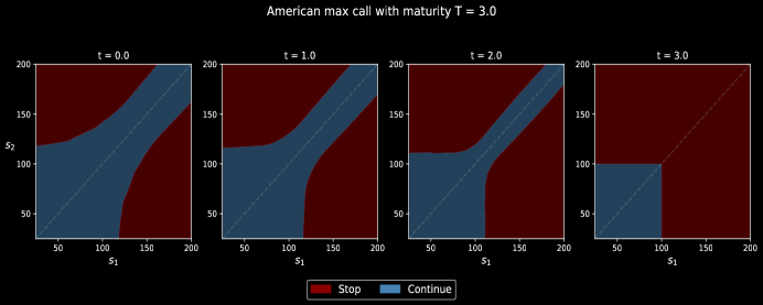
Figure 3: Evolution of the Free Boundary with $S_{0}=100$

5 Valuation and Hedging

We consider a European option with stock process $S$ and pay-off $\varphi(S_{T})$. We consider the Heston dynamics,

$$\mathrm{d}S_{t} =S_{t}\,(\mu\mathrm{d}t+\sqrt{v_{t}\,}\,\mathrm{d}W_{t}),$$

$$\mathrm{d}v_{t} =\left(\kappa(\theta-v_{t})-\lambda\,v_{t}\right)\,\mathrm{d}t+\sigma\,v_{t}\,\mathrm{d}\tilde{W}_{t},$$

where $W,\tilde{W}$ are one-dimensional Brownian motions with constant correlation of $\rho$, and the five Heston parameters $(\mu,\kappa,\theta,\sigma,\rho)$ are chosen satisfying the Feller condition. In particular, we choose the market price of volatility risk parameter $\lambda$.

Let $p^{*}$ be the price of this claim, and $Z$ be the return process, i.e.,

$$Z_{t+1}:=\frac{S_{t+1}-S_{t}}{S_{t}},\qquad t\in{\mathcal{T}}.$$ (5.1)

Further, let the feedback actions be the continuous functions

$$\pi:{\mathcal{T}}\times\mathbb{R}_{+}\times\mathbb{R}\ \mapsto\ \mathbb{R},$$

representing the dollar amount invested in the stock. The corresponding wealth process is given by,

$$X^{\pi,x}_{t+1}=(1+r)\,X^{\pi,x}_{t}+\pi(t,X^{\pi,x}_{t},Z_{t})\,\left(Z_{t+1}-r\,\right),\quad t\in{\mathcal{T}},$$ (5.2)

with initial data $X^{\pi,x}_{0}=x$.

We first fix an initial wealth of $x<p^{*}$ and consider the following pure-hedging problem of minimizing the square hedging error, i.e.,

$$v^{*}(x):=\min_{\pi\in{\mathcal{C}}}\,v(x,\pi),\qquad\text{where}\qquad v(x,\pi):=\mathbb{E}\left[(\varphi(S_{T})-X^{\pi,x}_{T})^{2}\ \right].$$ (5.3)

In the second problem, we minimize over $x$ as well, i.e,

$$v^{*}:=\min_{x\in\mathbb{R}}\,v^{*}(x)=\min_{(x,\pi)\in\mathbb{R}\times{\mathcal{C}}}\,v(x,\pi).$$ (5.4)

As proved by Föllmer & Schweizer [18], it is well-known that in continuous time the solution to the second problem, $v^{*}$, is equal to the Heston price. Thus, for sufficiently fine discretization $v^{*}$ is close to zero, $x^{*}$ is close to the known continuous-time Heston price. Also the numerical hedge $\pi^{*}$ must be equal to the continuous time hedge.

If $r=0$, then, $X^{\pi,x}_{t}=x+X^{\pi,0}_{t}$ and the initial wealth $x$ only influences the mean of the hedging error. Therefore, we expect that after an initial adjustment to minimize the mean, the networks would minimize the variance which is independent of the initial wealth. This approximate reasoning indicates that after an initial transient region, both minimization problems may behave similarly when there is large data.

5.1 Numerical results

We implemented the above hedging problem in Julia’s Flux [27] by parameterizing the portfolio at each time point, including the initial wealth level. In particular, we hedge a call option with strike $K$, i.e., $\varphi(x)=(x-K)_{+}=\max\{x-K,0\}$. Our implementation follows the scheme in Section 3, which we here describe in greater detail for this particular problem.

We see in (5.4) that the two quantities we optimize over are $x$ and $\pi$. As $x$ is a scalar, we directly parameterize it with a 1-element tensor, which after optimization is the option price. The policy $\pi$, however, can be approximated in various ways. We here opt for a very direct method in which we represent it by a single neural network with time and stock data as inputs. This contrasts [9], where the authors discretize time and design one neural network per time point. As we shall see, our implementation of a single neural network also performs well, with the additional benefit of allowing changes to the time discretization during training. There are also other training differences between the two parameterizations, as, for instance, the one used here accomplishes a large degree of parameter sharing. Nevertheless, a thorough account of these differences is outside the scope of the present paper.

Another detail of our implementation is that we write $\pi$ as a function of $t$ and $S_{t}$ instead of the formulation in (5.2). It is clear that the two are mathematically equivalent, although they could differ in training performance. Ours is a naïve choice and we make it because we find it more natural, not because it necessarily leads to better performance. The neural network is designed with two hidden layers of width 20 and with ReLU activation. In-between layers, batch normalization is employed.

The results of our computations are presented in Table 3. We compare our numerical solution to the Heston prices from https://www.quantlib.org/. No significant tuning has gone into producing our values, and it is nevertheless clear that accurate prices are consistently attained. We see, for instance, that the absolute error is approximately the same for all three strikes, which we argue is a consequence of (i) not tuning the training parameters to each individual problem and (ii) our hedging is in discrete time, which introduces a time discretization error. Although this is only a one-dimensional problem, it gives credence to the method’s effectiveness, effectiveness that does translate into higher-dimensional performance, as we illustrated for the American options problems.

$K$	QuantLib price	Price	Avg. abs. error	Error std. dev.
90	10.076508	10.078163	0.001869	0.001174
100	2.295405	2.295211	0.002018	0.001065
110	0.128136	0.127069	0.001971	0.001793

Table 3: Hedging performance of a call option with strike $K$ in a Heston model with parameters $S_{0}=100$, $v_{0}=0.04$, $\kappa=0.9$, $\theta=0.04$, $r=\lambda=0$ and $\sigma=0.2$. The maturity $T=1/12$ and the time interval is discretized in 22 steps. Each row lists the deep hedging price average over 100 runs along with the standard deviation over the same 100 runs.

Theoretically, in continuous-time, the optimal hedge is independent of the initial wealth. We also studied this by fixing the initial portfolio value to the price and also to its half value. One simulation of the trained hedge is given in the Figure 4 shows that the dependence is minimal.

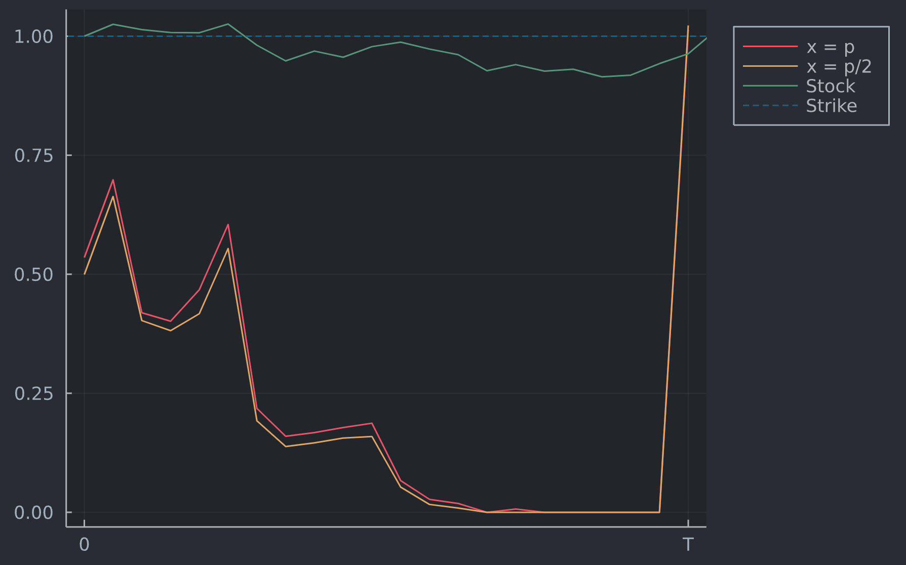
Figure 4: Optimal Hedges for the Heston model. The orange curve is the trained feedback hedge with an initial wealth half the option price, while the red curve is trained with initial wealth equal to the option price. The stock price is rescaled to start at $S_{0}=1$.

6 Merton Problem and Overlearning

In this section, we summarize the results of [31] by the first two authors. As in that paper, to emphasize the essential features of the algorithm, a simple financial market without any frictions and constant coefficients is considered. Additionally, consumption is not taken into account. All these details can incorporated into the model and problems with complex market structures have already been studied extensively by Buehler et.al. [9, 10].

Consider a stock price process $S_{t}\in\mathbb{R}_{+}^{d}$ in discrete time and assume a constant interest rate of $r$. Let the return process $Z$ be as in (5.1) and $X^{\pi}=X^{\pi,x}$ be as in (5.2). We suppress the dependence of the initial wealth $x$ for simplicity. Then, the classical investment problem is to maximize $v(\pi):=\mathbb{E}[U(X^{\pi}_{T})]$ with a given utility function $U$.

In [31] it is proved that the deep empirical risk minimization algorithm converges as the size of the training data gets larger. On the other hand, it is also shown that for fixed training data sets, larger and deeper neural networks have the capability of overlearning the data, however large it might be. In such situations, the trained neural networks while substantially over-perform the theoretical optimum on the training set, they do not generalize and perform poorly on other data sets.

These theoretical results are demonstrated in the following stylized example with an explicit solution in [31](Section 8). In that example, the utility function is taken to be the exponential with parameter one, and as the decisions are independent of the initial value for these class of utilities, the initial value is fixed as one dollar. To simplify even further, for one period this amount is invested uniformly on all stocks. Then, with ${\bf{1}}:=(1,\ldots,1)$, $\pi_{0}={\bf{1}}/d$ and $X_{1}=(Z_{1}\cdot{\bf{1}})/d-r$ are uncontrolled, and the investment problem is to choose the feedback portfolio $\pi_{1}(Z_{1})\in\mathbb{R}^{d}$ so as to maximize

$$v(\pi)=\mathbb{E}\big{[}1-\exp(-X^{\pi}_{2})\big{]},$$

where $X^{\pi}_{2}=(1+r)X_{1}+a(Z_{1})\cdot(Z_{2}-r{\bf{1}})$. The certainty equivalent of a utility value $v<1$ given by

$$\mathrm{ce}(v):=\ln(1-v)\quad\Longleftrightarrow\quad v=U(\mathrm{ce}(v))$$

is a more standard way of comparing different utility values. Indeed, agents with expected utility preferences would be indifferent between an action $\pi$ and a cash amount of $\mathrm{ce}(v(\pi))$ because the utilities of both positions are equal to each other. Thus, for these agents the cash equivalent of the action $\pi$ is $\mathrm{ce}(v(\pi))$.

The following table [31](Table 1) clearly demonstrates overlearning. In this experiments the training data of size $N=100,000$ and an artificial neural network with three hidden layers of width 10 is trained on this set for four or five epochs. For each dimension the algorithm is run thirty times and Table 4 below reports the mean and the standard. deviation. Although conservative stopping rules are employed in [31], there is substantial overperformance increasing with dimension.

dims	$p_{in}$ (%)		$p_{in}-p_{out}$ (%)
	$\mu\ \quad$	$\sigma\ \quad$	$\mu\ \quad$	$\sigma\ \quad$
100	10.12820	1.09290	23.67080	2.01177
85	8.38061	1.35575	20.16440	2.30489
70	7.32720	0.86458	15.62060	1.94043
55	5.05783	0.81518	10.93950	1.54431
40	3.74648	0.62588	7.91105	1.32581
25	2.11501	0.43845	4.58954	0.88461
10	0.53982	0.34432	1.46138	0.39078

Table 4: Average relative in-sample performance, and its comparison to the out-of-sample performance with the above described conservative stopping rule. Everything is in % with training size of $N=100,000$ and three hidden layers of width 10. The $\mu$ value is the average of 30 runs and $\sigma$ is the standard deviation.

7 Conclusion

The deep empirical risk minimization proposed by E, Han & Jentzen [21, 22] provides a flexible and a highly effective tool for stochastic optimization problems arising in computational finance. Recent development of optimization libraries make this algorithm tractable in very high dimensions allowing to include important market details such as factors and frictions, as well as models with long memory. Once a large training set is given, the algorithm mimics the market dynamics with all its details. This simple description together with powerful new computational tools are keys to the power of the algorithm. We have demonstrated above properties in three different classes of problems. As it is always the case, each requires problem specific but natural modifications. Moreover, the output can be designed to be exactly the decision rule that is under investigation.

The method on the other hand needs large data sets for reliable results. In the financial setting this essentially limits its scope to model driven markets with an unlimited simulation capability. However, due to its seamless transition to more complex structures, more interesting parametric models are now feasible. Thus, on-going research on market generators will be an important factor on further developments.

References

- Andersen and Broadie [2004] L. Andersen and M. Broadie. Primal-dual simulation algorithm for pricing multidimensional American options. Management Science, 50(9):1222–1234, 2004.
- Bachouch et al. [2018] A. Bachouch, C. Huré, N. Langrené, and H. Pham. Deep neural networks algorithms for stochastic control problems on finite horizon, part 2: Numerical applications. arXiv:1812.05916, 2018.
- Bayer et al. [2020] C. Bayer, R. Tempone, and S. Wolfers. Pricing American options by exercise rate optimization. Quantitative Finance, 20(11):1749–1760, 2020.
- Becker et al. [2019] S. Becker, P. Cheridito, and A. Jentzen. Deep optimal stopping. Journal of Machine Learning Research, 20(4):1–25, 2019.
- Becker et al. [2021] S. Becker, P. Cheridito, A. Jentzen, and T. Welti. Solving high-dimensional optimal stopping problems using deep learning. European Journal of Applied Mathematics, 32(3):470–514, 2021.
- Bertsekas and Tsitsiklis [1996] D. Bertsekas and J. Tsitsiklis. Neuro-dynamic programming. Athena Scientific, 1996.
- Boudabsa and Filipović [2021] L. Boudabsa and D. Filipović. Machine learning with kernels for portfolio valuation and risk management. Finance and Stochastics, pages 1–42, 2021.
- Broadie and Detemple [1997] M. Broadie and J. Detemple. The valuation of American options on multiple assets. Mathematical Finance, 7(3):241–286, 1997.
- Buehler et al. [2019a] H. Buehler, L. Gonon, J. Teichmann, and B. Wood. Deep hedging. Quantitative Finance, 19(8):1271–1291, 2019a.
- Buehler et al. [2019b] H. Buehler, L. Gonon, J. Teichmann, B. Wood, and B. Mohan. Deep hedging: hedging derivatives under generic market frictions using reinforcement learning. Technical report, Swiss Finance Institute, 2019b.
- Chevalier et al. [2021] E. Chevalier, S. Pulido, and E. Zúñiga. American options in the Volterra Heston model. arXiv:2103.11734, 2021.
- Ciocan and Mišić [2022] D. Ciocan and V. Mišić. Interpretable optimal stopping. Management Science, 68(3):1616–1638, 2022.
- Cybenko [1989] G. Cybenko. Approximations by superpositions of a sigmoidal function. Mathematics of Control, Signals and Systems, 2:183–192, 1989.
- Detemple [2005] J. Detemple. American-style derivatives: Valuation and computation. CRC Press, 2005.
- Fecamp et al. [2020] S. Fecamp, J. Mikael, and X. Warin. Deep learning for discrete-time hedging in incomplete markets. Journal of computational Finance, 2020.
- Filipovic et al. [2021] D. Filipovic, M. Multerer, and P. Schneider. Adaptive joint distribution learning. arXiv:2110.04829, 2021.
- Fleming and Soner [2006] W. H. Fleming and H. M. Soner. Controlled Markov processes and viscosity solutions, volume 25. Springer Science & Business Media, 2006.
- Föllmer and Schweizer [1991] H. Föllmer and M. Schweizer. Hedging of contingent claims under incomplete information. Applied stochastic analysis, 5(389-414):19–31, 1991.
- Germain et al. [2020] M. Germain, H. Pham, and X. Warin. Deep backward multistep schemes for nonlinear pdes and approximation error analysis. arXiv:2006.01496, 2020.
- Gonon et al. [2021] L. Gonon, J. Muhle-Karbe, and X. Shi. Asset pricing with general transaction costs: Theory and numerics. Mathematical Finance, 31(2):595–648, 2021.
- Han and E [2016] J. Han and W. E. Deep learning approximation for stochastic control problems. In Deep Reinforcement Learning Workshop, NIPS, 2016.
- Han et al. [2018] J. Han, A. Jentzen, and W. E. Solving high-dimensional partial differential equations using deep learning. Proceedings of the National Academy of Sciences, 115(34):8505–8510, 2018.
- Heston [1993] S. L. Heston. A closed-form solution for options with stochastic volatility with applications to bond and currency options. The Review of Financial Studies, 6(2):327–343, 1993.
- Hornik [1991] K. Hornik. Approximation capabilities of multilayer feedforward networks. Neural networks, 4(2):251–257, 1991.
- Huré et al. [2018] C. Huré, H. Pham, A. Bachouch, and N. Langrené. Deep neural networks algorithms for stochastic control problems on finite horizon, part I: convergence analysis. arXiv:1812.04300, 2018.
- Hutchinson et al. [1994] J. M. Hutchinson, A. W. Lo, and T. Poggio. A nonparametric approach to pricing and hedging derivative securities via learning networks. The Journal of Finance, 49(3):851–889, 1994.
- Innes [2018] M. Innes. Flux: Elegant machine learning with julia. Journal of Open Source Software, 3(25):602, 2018.
- Laurière et al. [2021] M. Laurière, G. Pagès, and O. Pironneau. Performance of a Markovian neural network versus dynamic programming on a fishing control problem. arXiv:2109.06856, 2021.
- Longstaff and Schwartz [2001] F. A. Longstaff and E. S. Schwartz. Valuing American options by simulation: a simple least-squares approach. The Review of Financial Studies, 14(1):113–147, 2001.
- Ludkovski [2020] M. Ludkovski. mlosp: Towards a unified implementation of regression Monte Carlo algorithms. arXiv:2012.00729, 2020.
- Reppen and Soner [2020] A. M. Reppen and H. M. Soner. Deep empirical risk minimization in finance: an assessment. in preparation, 2020.
- Reppen et al. [2022] A. M. Reppen, H. M. Soner, and V. Tissot-Daguette. Neural optimal stopping boundary. in preparation, 2022.
- Ruf and Wang [2020a] J. Ruf and W. Wang. Hedging with neural networks. arXiv:2004.08891, 2020a.
- Ruf and Wang [2020b] J. Ruf and W. Wang. Neural networks for option pricing and hedging: a literature review. Journal of Computational Finance, 24(1), 2020b.
- Schweizer [1991] M. Schweizer. Option hedging for semimartingales. Stochastic Processes and Their Applications, 37(2):339–363, 1991.
- Schweizer [1999] M. Schweizer. A guided tour through quadratic hedging approaches. Technical report, SFB 373 Discussion Paper, 1999.
- Sirignano and Spiliopoulos [2018] J. Sirignano and K. Spiliopoulos. Dgm: A deep learning algorithm for solving partial differential equations. Journal of Computational Physics, 375:1339–1364, 2018.
- Tsitsiklis and Van Roy [2001] J. N. Tsitsiklis and B. Van Roy. Regression methods for pricing complex American-style options. IEEE Transactions on Neural Networks, 12(4):694–703, 2001.
- Wang and Perdikaris [2021] S. Wang and P. Perdikaris. Deep learning of free boundary and Stefan problems. Journal of Computational Physics, 428:109914, 2021.
- Warin [2019] X. Warin. Variance optimal hedging with application to electricity markets. Journal of Computational Finance, 23(3):33–59, 2019.