A Unified Model for Reverse Dictionary and Definition Modelling

Abstract

We build a dual-way neural dictionary to retrieve words given definitions, and produce definitions for queried words. The model learns the two tasks simultaneously and handles unknown words via embeddings. It casts a word or a definition to the same representation space through a shared layer, then generates the other form in a multi-task fashion. Our method achieves promising automatic scores on previous benchmarks without extra resources. Human annotators prefer the model’s outputs in both reference-less and reference-based evaluation, indicating its practicality. Analysis suggests that multiple objectives benefit learning.

1 Introduction

A monolingual dictionary is a large-scale collection of words paired with their definitions. The main use of such a resource is to find a word or a definition having known the other. Formally, the task of generating a textual definition from a word is named definition modelling; the inverse task of retrieving a word given a definition is called reverse dictionary. Lately, the two tasks are approached using neural networks (Hill et al., 2016; Noraset et al., 2017), and in turn they help researchers better understand word sense and embeddings. Research can further benefit low-resource languages where high-quality dictionaries are not available (Yan et al., 2020). Finally, practical applications include language education, writing assistance, semantic search, etc.

While previous works solve one problem at a time, we argue that both tasks can be learned and dealt with concurrently, based on the intuition that a word and its definition share the same meaning. We design a neural model to embed words and definitions into a shared semantic space, and generate them from this space. Consequently, the training paradigm can include reconstruction and embedding similarity tasks. Such a system can be viewed as a neural dictionary that supports two-way indexing and querying. In our experiments, jointly learning both tasks does not increase the total model size, yet demonstrates ease and effectiveness. Our code is publicly available.

2 Related Work

Although research on the two tasks can be traced back to the early 2000s, recent research has shifted towards neural networks, which we describe here.

Reverse dictionary

Hill et al. (2016) pioneer the use of RNN and bag-of-words models to convert texts to word vectors, on top of which Morinaga and Yamaguchi (2018) add an extra word category classifier. Pilehvar (2019) integrates super-sense into target embeddings to disambiguate polysemous words. Zhang et al. (2020) design a multi-channel network to predict a word with its features like category, POS tag, morpheme, sememe, etc.

Nonetheless, our work tackles the problem without using linguistically annotated resources. The proposed framework learns autoencodings for definitions and words, instead of mapping texts to plain word vectors. From this aspect, Bosc and Vincent (2018) train word embeddings via definition reconstruction.

Definition modelling

Noraset et al. (2017) use RNNs for definition generation, followed by Gadetsky et al. (2018) who add attention and word context, as well as Chang et al. (2018) whose model projects words and contexts to a sparse space, then generates from selected dimensions only. Mickus et al. (2019)’s model encodes a context sentence and marks the word of interest, whereas Bevilacqua et al. (2020)’s defines a flexible span of words. Apart from generating definitions freely, Chang and Chen (2019) take a new perspective of re-formulating the generation task to definition retrieval from a dictionary.

3 Methodology

3.1 A unified model with multi-task training

A word (embedding) and its definition share the same meaning, even though they exist in different surface forms. When we model their semantics using a neural method, we hypothesize that a word and its definition can be encoded into a consistent representation space. This gives rise to our core architecture in the paper: a model that transforms inputs into a shared embedding space that can represent both words and definitions. We then have downstream modules that convert the shared embeddings back to words or definitions. Essentially, the shared representation can be viewed as an autoencoding of the meaning of a word and its definition. In the learning process, definition modelling and reverse dictionary are jointly trained to aid each other; yet at inference time, only half of the network needs to be used to perform either task.

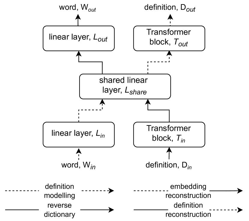
Figure 1: An illustration of our designed model.

The proposed architecture with four sub-task workflows is illustrated in Figure 1. The autoencoding capability is accomplished through a shared linear layer L_share between the encoder and the decoder networks, the output of which is the encoded words and definitions. We use linear layers L_in and L_out to process words W_in and W_out before and after the shared layer. Likewise, we have definitions D_in and D_out converted to and from the shared layer, using Transformer blocks T_in and T_out (Vaswani et al., 2017). In addition, we encourage the shared layer’s representations of the input word W_in and definition D_in to be as close as possible. The Transformer blocks operate on self-attention but not encoder-decoder attention, i.e. Transformer blocks do not attend to each other, so as to force all information to flow through the autoencoding bottleneck.

With an embedding distance $\mathrm{embed\_dist()}$ and a token-level loss $\mathrm{token\_loss()}$, canonical reverse dictionary and definition modelling have losses:

$$\mathcal{L}_{\mathrm{revdic}}= \mathrm{embed\_dist}(\mathrm{W}_{\mathit{gold}},\mathit{L}_{\mathit{out}}(\mathit{L}_{\mathit{share}}(\mathit{T}_{\mathit{in}}(\mathrm{D}_{\mathit{in}}))))$$

$$\mathcal{L}_{\mathrm{defmod}}= \mathrm{token\_loss}(\mathrm{D}_{\mathit{gold}},\mathit{T}_{\mathit{out}}(\mathit{L}_{\mathit{share}}(\mathit{L}_{\mathit{in}}(\mathrm{W}_{\mathit{in}}))))$$

Our model also optimizes on the losses from word and definition reconstruction (autoencoding):

$$\mathcal{L}_{\mathrm{wordAE}}= \mathrm{embed\_dist}(\mathrm{W}_{\mathit{gold}},\mathit{L}_{\mathit{out}}(\mathit{L}_{\mathit{share}}(\mathit{L}_{\mathit{in}}(\mathrm{W}_{\mathit{in}}))))$$

$$\mathcal{L}_{\mathrm{defAE}}= \mathrm{token\_loss}(\mathrm{D}_{\mathit{gold}},\mathit{T}_{\mathit{out}}(\mathit{L}_{\mathit{share}}(\mathit{T}_{\mathit{in}}(\mathrm{D}_{\mathit{in}}))))$$

The distance between a pair of word and definition representations from the shared layer is:

$$\mathcal{L}_{\mathrm{sim}}=\mathrm{embed\_dist}(\mathit{L}_{\mathit{share}}(\mathit{T}_{\mathit{in}}(\mathrm{D}_{\mathit{in}})),\mathit{L}_{\mathit{share}}(\mathit{L}_{\mathit{in}}(\mathrm{W}_{\mathit{in}})))$$

Finally, our training minimizes the overall loss $\mathcal{L}$ that adds all above losses weighted equally:

$$\mathcal{L}=\mathcal{L}_{\mathrm{revdic}}+\mathcal{L}_{\mathrm{defmod}}+\mathcal{L}_{\mathrm{wordAE}}+\mathcal{L}_{\mathrm{defAE}}+\mathcal{L}_{\mathrm{sim}}$$

3.2 Word-sense disambiguation

A word is often associated with multiple definitions due to the presence of polysemy, sense granularity, etc. In our practice, the one-to-many word-definition relationship does not harm reverse dictionary, since our model can master mapping different definitions into the same word vector. However, it is problematic for definition modelling, as telling the exact word sense without context is hard. Thus, we embed words in their usage context (supplied in the data we use) using BERT (Devlin et al., 2019). We sum up the sub-word embeddings for each word if it is segmented by BERT.

4 Experiments and Results

4.1 Data and evaluation

Hill: we evaluate reverse dictionary on Hill et al. (2016)’s English data. There are roughly 100k words and 900k word-definition pairs. Three test sets are present to test a system’s memorizing and generalizing capabilities: 500 seen from training data, 500 unseen, and 200 human description (where definitions are from a human, instead of a dictionary). The evaluation metrics are retrieval accuracies at 1, 10 and 100, as well as the median and standard deviation of the target words’ ranks.

Chang: definition modelling is experimented on Chang and Chen (2019)’s data from the Oxford English Dictionary. Each instance is a tuple of a word, its usage (context), and a definition. The data has two splits: seen and unseen. The unseen split we use consists of 530k training instances, and the test set is 1k words paired with 16.0k definitions and context. Performance is measured by corpus-level Bleu from Nltk, and Rouge-L F1 (Papineni et al., 2002; Lin, 2004; Bird et al., 2009).

	unseen				human description
	median rank	acc@ 1/10/100	rank std.†	real std.	median rank	acc@ 1/10/100	rank std.†	real std.
OneLook.com	-	-	-	-	5.5	.33/.54/.76	332	-
bag-of-words	248	.03/.13/.39	424	-	22	.13/.41/.69	308	-
RNN	171	.03/.15/.42	404	-	17	.14/.40/.73	274	-
category inference	170	.05/.19/.43	420	-	16	.14/.41/.74	306	-
multi-sense	276	.03/.14/.37	426	-	1000	.01/.04/.18	404	-
super-sense	465	.02/.11/.31	454	-	115	.03/.15/.47	396	-
multi-channel	54	.09/.29/.58	358	-	2	.32/.64/.88	203	-
Transformer	79	.01/.14/.59	473	125	27	.05/.23/.87	332	49
unified	18	.13/.39/.81	386	93	4	.22/.64/.97	183	30
+ share embed	20	.08/.36/.77	410	99	4	.23/.65/.97	183	32

Table 1: Reverse dictionary results on the Hill data with past results from Zhang et al. (2020)’s re-run. ^†They force-set a word rank larger than 100 to 1000 which affected std.; we follow suit for comparison, and also include the real std.

4.2 The questionable seen test set

Understandably, a dictionary needs to “memorize” word entries, so both Hill and Chang supply a seen test drawn from training data. However, this is impractical in deep learning, for it implicitly encourages overfitting. Further, the foremost function of a neural dictionary is to deal with unseen words and definitions; otherwise, a traditional rule-based one suffices. We hence omit evaluation on seen sets and request future research to not focus on it.

4.3 System configurations

Our baselines are 4-layer Transformer blocks: a Transformer encoder for reverse dictionary, and a Transformer decoder for definition modelling. Hyperparameter searches are detailed in Appendix A. We tokenize training definitions into an open vocabulary by whitespace. We use cross-entropy for definition tokens and mean squared error (MSE) as the embedding distance.

Our proposed model essentially connects and trains the above two baselines with an extra shared layer. The layer has the same size as the input embeddings and a residual connection (He et al., 2016). As an additional variant, we tie both Transformer blocks’ embedding and output layers (Press and Wolf, 2017). This is only possible with our multi-task framework, since a Transformer block baseline does not have both encoder and decoder embeddings. The unified model optimizes roughly twice as many parameters as a single-task baseline; in other words, when performing both tasks, our system is of the same size as the baseline models.

For reverse dictionary, we compare with a number of existing works: OneLook.com, bag-of-words, RNN (Hill et al., 2016), category inference (Morinaga and Yamaguchi, 2018), multi-sense (Kartsaklis et al., 2018), super-sense (Pilehvar, 2019) and multi-channel Zhang et al. (2020). Following Zhang et al. (2020) we embed target words with 300d word2vec (Mikolov et al., 2013), but definition tokens are encoded into 256d embeddings to train from scratch, instead of pre-trained embeddings.

For definition modelling, words are embedded by 768d BERT-base-uncased, while definition token embeddings are initialized randomly. We include RNN (Noraset et al., 2017) and xSense (Chang et al., 2018) for reference but not Chang and Chen (2019)’s results from an oracle retrieval experiment.

Our choice of word embedders aligns with previous works, which ensures that comparison is fair and improvement comes from the model design. It is also worth noting that we train separate models on HILL and CHANG data to evaluate reverse dictionary and definition modelling performances respectively.

4.4 Results

Reverse dictionary

results in Table 1 show a solid baseline, which our proposed models significantly improve upon. Compared to previous works, we obtain the best ranking and accuracies on unseen words. On human descriptions our models yield compelling accuracies with the best standard deviation, indicating a consistent performance.

One highlight is that our model attains a superior position without linguistic annotations, other than a word embedder which is always used in previous research. Consequently, ours can be concluded as a more generic framework for this task.

Definition modelling

results are reported in Table 2. On the unseen test, our model with tied embeddings achieves state-of-the-art scores. The model without it has performance similar to the baseline. Admittedly, while Rouge-L scores look reasonable, the single-digit Bleu might hint at the poor quality of the generation. We conduct human evaluation and discuss that later.

	unseen
	Bleu	Rouge-L
RNN	1.7	15.8
xSense	2.0	15.9
Transformer	2.4	17.9
unified	2.2	18.5
+ share embed	3.0	20.2

Table 2: Definition modelling results on the Chang data, with past numbers from Chang and Chen (2019)’s replicate.

5 Analysis and Discussions

5.1 Shared embeddings and the vocabulary

For definition modelling, a shared embedding and output layer brings significant improvement to our proposed approach, but in reverse dictionary, our models arrive at desirable results without it. This is reasonable as well-trained embedding and output layers particularly benefit language generation (Press and Wolf, 2017). It further indicates the usefulness of our unified approach whereby all embedding and output layers can be weight-tied, enabled by concurrently training the two Transformer sub-models for the two tasks.

We have used an open vocabulary, which has weaknesses like being oversized and vulnerable to unknown tokens. Therefore, we add a model with a 25k unigram SentencePiece vocabulary (Kudo and Richardson, 2018) to definition modelling. All other configurations remain the same as the best-performing model. Bleu and Rouge-L drop to 2.5 and 18.7, proving that an open vocabulary is not an issue in our earlier experiments.

5.2 Human evaluation on definitions

Supplementary to the automatic evaluation for definition generation, we run reference-less and reference-based human evaluation, on the Transformer baseline and the best-performing unified model. In a reference-less evaluation, a human is asked to pick the preferred output after seeing a word, whereas in a reference-based setting, a human sees a reference definition instead. Test instances are sampled, and then the models’ outputs are presented in a shuffled order. Two annotators in total evaluated 80 test instances for each setting. Table 3 records the number of times each model is favoured over the other.

Regardless of the evaluation condition, evaluators often regard the unified model’s outputs as better. Especially in the reference-less scenario, which resembles a real-life application of definition generation, our unified model wins notably.

	reference-less	reference-based
Transformer	25 (31%)	32 (40%)
unified	50 (63%)	42 (53%)

Table 3: Chances a model’s output is preferred by human evaluators. Columns do not add up to 80 (100%) because we do not count when both models generated the same output.

5.3 Ablation studies on the objectives

Our models are trained with five losses from five tasks: definition modelling, reverse dictionary, two reconstruction tasks and a shared embedding similarity task. In contrast to the full 5-task model, we try to understand how multiple objectives influence learning, by excluding certain losses.

We first remove reconstruction losses to form a 3-task model that learns reverse dictionary, definition modelling and embedding similarity. This is the minimum set of tasks required to train the full architecture and to ensure words and definitions are mapped to the same representation. Then we designate 1-task models to learn either reverse dictionary or definition modelling depending on the baseline it is compared to. Such a model is deeper than the baseline Transformer but partly untrained.

We run the ablation investigation on both reverse dictionary and definition modelling tasks. We log training dynamics in Figure 2: embedding MSE against epochs for reverse dictionary, and generation cross-entropy against epochs for definition modelling. The curve plotting stops when validation does not improve.

Figure 2: Validation losses (y-axis) against epochs (x-axis).

As Figure 2a shows, the single-task Hill model does not converge, probably because in reverse dictionary the Transformer block is far away from the output end, and only receives small gradients from just one loss. The 3-task and 5-task models display similar losses, but the 3-task loss curve is smoother. In Figure 2b for definition modelling, the 3-task model trains the fastest, but 1-task and 5-task models reach better convergence. It implies that learning more than one task is always beneficial compared to single-task training; reconstruction is sometimes helpful but not crucial.

6 Conclusion

We build a multi-task model for reverse dictionary and definition modelling. The approach records strong numbers on public datasets. Our method delegates disambiguation to BERT and minimizes dependency on linguistically annotated resources, so it can potentially be made cross-lingual and multilingual. A limitation is that the current evaluation centers on English, without exploring low-resource languages, which could be impactful extensions that benefit the community.

Appendix A Hyperparameters and Computation

Our model configuration search is summarized here. We adjusted the hyperparameters for the baseline using the validation set, and kept the values unchanged for the proposed model which joins two baseline Transformer blocks. We list all hyperparameters in Table 4, and highlight the selected ones in bold if multiple values were tried out. The trial is carried out one by one for each hyperparameter. On a single Nvidia GeForce GTX 1080 Ti, it takes 60 hours for a reverse dictionary model to converge; a definition modelling model converges after 6 hours on a single Nvidia GeForce RTX 2080 Ti.

word embed.	Hill: word2vec
	Chang: BERT-base-uncased
word embed. dim.	Hill: 300
	Chang: 768
definition tokenizer	whitespace
def. token embed.	none, trained from one-hot
def. token embed. dim.	256
training toolkit	PyTorch (Paszke et al., 2019)
stopping criterion	5 non-improving validations
learning rate	1e-3, 1e-4, 1e-5 and 1e-6
optimizer	Adam (Kingma and Ba, 2015)
beta1, beta2	0.9, 0.999
weight decay	1e-6
embedding loss	MSE, cosine (failed to converge)
token loss	cross-entropy
training batch size	Hill: 256
	Chang: 128
decoding batch size	1
decoding beam size	6, 64
Transformer depth	4, 6
Transformer head	4, 8
Transformer dropout	0.1, 0.3
def. token dropout	0, 0.1
linear layer dropout	0.2
linear layer dim.	Hill: 256
	Chang: 768
shared layer dim.	Hill: 256
	Chang: 768
trainable parameters	Hill: 35.1M
	Chang: 62.7M

Table 4: Model and training configurations.

References

- Bevilacqua et al. (2020) Michele Bevilacqua, Marco Maru, and Roberto Navigli. 2020. Generationary or “how we went beyond word sense inventories and learned to gloss”. In Proceedings of EMNLP, pages 7207–7221, Online. Association for Computational Linguistics.
- Bird et al. (2009) Steven Bird, Ewan Klein, and Edward Loper. 2009. Natural Language Processing with Python. O’Reilly Media.
- Bosc and Vincent (2018) Tom Bosc and Pascal Vincent. 2018. Auto-encoding dictionary definitions into consistent word embeddings. In Proceedings of EMNLP, pages 1522–1532, Brussels, Belgium. Association for Computational Linguistics.
- Chang and Chen (2019) Ting-Yun Chang and Yun-Nung Chen. 2019. What does this word mean? explaining contextualized embeddings with natural language definition. In Proceedings of EMNLP-IJCNLP, pages 6064–6070, Hong Kong, China. Association for Computational Linguistics.
- Chang et al. (2018) Ting-Yun Chang, Ta-Chung Chi, Shang-Chi Tsai, and Yun-Nung Chen. 2018. xSense: Learning sense-separated sparse representations and textual definitions for explainable word sense networks. arXiv.
- Devlin et al. (2019) Jacob Devlin, Ming-Wei Chang, Kenton Lee, and Kristina Toutanova. 2019. BERT: Pre-training of deep bidirectional transformers for language understanding. In Proceedings of NAACL, pages 4171–4186, Minneapolis, Minnesota. Association for Computational Linguistics.
- Gadetsky et al. (2018) Artyom Gadetsky, Ilya Yakubovskiy, and Dmitry Vetrov. 2018. Conditional generators of words definitions. In Proceedings of ACL, pages 266–271, Melbourne, Australia. Association for Computational Linguistics.
- He et al. (2016) Kaiming He, Xiangyu Zhang, Shaoqing Ren, and Jian Sun. 2016. Deep residual learning for image recognition. In CVPR, pages 770–778.
- Hill et al. (2016) Felix Hill, Kyunghyun Cho, Anna Korhonen, and Yoshua Bengio. 2016. Learning to understand phrases by embedding the dictionary. TACL, 4:17–30.
- Kartsaklis et al. (2018) Dimitri Kartsaklis, Mohammad Taher Pilehvar, and Nigel Collier. 2018. Mapping text to knowledge graph entities using multi-sense LSTMs. In Proceedings of EMNLP, pages 1959–1970, Brussels, Belgium. Association for Computational Linguistics.
- Kingma and Ba (2015) Diederik P. Kingma and Jimmy Ba. 2015. Adam: A method for stochastic optimization. In ICLR.
- Kudo and Richardson (2018) Taku Kudo and John Richardson. 2018. SentencePiece: A simple and language independent subword tokenizer and detokenizer for neural text processing. In Proceedings of EMNLP, pages 66–71, Brussels, Belgium. Association for Computational Linguistics.
- Lin (2004) Chin-Yew Lin. 2004. ROUGE: A package for automatic evaluation of summaries. In Text Summarization Branches Out, pages 74–81, Barcelona, Spain. Association for Computational Linguistics.
- Mickus et al. (2019) Timothee Mickus, Denis Paperno, and Matthieu Constant. 2019. Mark my word: A sequence-to-sequence approach to definition modeling. In Proceedings of the First NLPL Workshop on Deep Learning for Natural Language Processing, pages 1–11, Turku, Finland. Linköping University Electronic Press.
- Mikolov et al. (2013) Tomás Mikolov, Kai Chen, Greg Corrado, and Jeffrey Dean. 2013. Efficient estimation of word representations in vector space. In ICLR Workshop.
- Morinaga and Yamaguchi (2018) Yuya Morinaga and Kazunori Yamaguchi. 2018. Improvement of reverse dictionary by tuning word vectors and category inference. In International Conference on Information and Software Technologies, pages 533–545, Cham. Springer International Publishing.
- Noraset et al. (2017) Thanapon Noraset, Chen Liang, Larry Birnbaum, and Doug Downey. 2017. Definition modeling: Learning to define word embeddings in natural language. In Proceedings of the AAAI Conference on Artificial Intelligence, pages 3259–3266.
- Papineni et al. (2002) Kishore Papineni, Salim Roukos, Todd Ward, and Wei-Jing Zhu. 2002. Bleu: a method for automatic evaluation of machine translation. In Proceedings of ACL, pages 311–318, Philadelphia, Pennsylvania, USA. Association for Computational Linguistics.
- Paszke et al. (2019) Adam Paszke, Sam Gross, Francisco Massa, Adam Lerer, James Bradbury, Gregory Chanan, Trevor Killeen, Zeming Lin, Natalia Gimelshein, Luca Antiga, Alban Desmaison, Andreas Kopf, Edward Yang, Zachary DeVito, Martin Raison, Alykhan Tejani, Sasank Chilamkurthy, Benoit Steiner, Lu Fang, Junjie Bai, and Soumith Chintala. 2019. Pytorch: An imperative style, high-performance deep learning library. In NeurIPS, pages 8024–8035. Curran Associates, Inc.
- Pilehvar (2019) Mohammad Taher Pilehvar. 2019. On the importance of distinguishing word meaning representations: A case study on reverse dictionary mapping. In Proceedings of NAACL, pages 2151–2156, Minneapolis, Minnesota. Association for Computational Linguistics.
- Press and Wolf (2017) Ofir Press and Lior Wolf. 2017. Using the output embedding to improve language models. In Proceedings of EACL, pages 157–163, Valencia, Spain. Association for Computational Linguistics.
- Vaswani et al. (2017) Ashish Vaswani, Noam Shazeer, Niki Parmar, Jakob Uszkoreit, Llion Jones, Aidan N. Gomez, Łukasz Kaiser, and Illia Polosukhin. 2017. Attention is all you need. In NeurIPS, pages 6000–6010.
- Yan et al. (2020) Hang Yan, Xiaonan Li, Xipeng Qiu, and Bocao Deng. 2020. BERT for monolingual and cross-lingual reverse dictionary. In Findings of EMNLP, pages 4329–4338, Online. Association for Computational Linguistics.
- Zhang et al. (2020) Lei Zhang, Fanchao Qi, Zhiyuan Liu, Yasheng Wang, Qun Liu, and Maosong Sun. 2020. Multi-channel reverse dictionary model. In Proceedings of AAAI, pages 312–319.