Neural Optimal Stopping Boundary

Abstract

A method based on deep artificial neural networks and empirical risk minimization is developed to calculate the boundary separating the stopping and continuation regions in optimal stopping. The algorithm parameterizes the stopping boundary as the graph of a function and introduces relaxed stopping rules based on fuzzy boundaries to facilitate efficient optimization. Several financial instruments, some in high dimensions, are analyzed through this method, demonstrating its effectiveness. The existence of the stopping boundary is also proved under natural structural assumptions.

Key words: Stopping boundary problems, American derivatives, Bermudan options, optimal stopping, deep learning, fuzzy boundary.
Mathematics Subject Classification: 91G20, 91G60, 68T07, 35R35.

1 Introduction

The classical decision problem of optimal stopping has found amazing range of applications from finance, statistics, marketing, phase transitions to engineering. While over the past decades many efficient methods have been developed for its numerical resolution, until recently essentially all computational approaches in high-dimensions first approximate the maximal value. The quantity that is equally important is the associated stopping rule, and the state is divided into two regions depending on whether at a point it is optimal to stop or to continue. Although approximate optimal actions can either be calculated directly, or are always available from the calculated value function in a greedy policy, a characterization and computation of these regions through interpretable criterion would provide an immediate link between the policy and the state.

In many important applications, continuation and stopping regions are separated by graphs of functions that can be used to construct interpretable optimal stopping decisions, and our goal is to directly compute these stopping boundaries whose performances are close to the maximal ones. In lower dimensions, they can be accurately approximated by methods based on nonlinear partial differential equations or dynamic programming. However, in models with many degrees of freedom, this numerical problem is still challenging.

Our approach is based on a method proposed by E, Jentzen & Han [32, 33], which we call deep empirical risk minimization (deep ERM). In this framework, the controller is replaced by a deep artificial neural network and the random system dynamics is simulated via Monte-Carlo. Recent advances in optimization tools and computational capabilities enable us to optimize this system efficiently, thus providing an accurate tool potentially also applicable to other problems with stopping boundaries, including models with regime change or other singularities in financial economics, phase transitions in continuum mechanics, and Stefan type problems in solidification.

Deep ERM applies essentially to all problems that can be formulated as dynamic stochastic optimization, maybe after problem specific modifications. This and similar algorithms [3, 7, 9, 10, 16, 17, 31, 2, 46, 48, 55] have been applied to many classical problems from quantitative finance, financial economics, and to nonlinear partial differential equations that have stochastic representations. Also, the application to optimal stopping is carried out by Becker, Jentzen & Cheridito [7, 9] to compute an approximation of the optimal stopping rule and hence, the stopping region as well as the maximal value. They accurately price many American options of practical importance in very high dimensions with confidence intervals, showcasing the power and the flexibility of deep ERM in optimal stopping as well. We refer the readers to our accompanying papers [43, 44] for an introduction of deep ERM, and to the excellent surveys [25, 35, 47] and the references therein for more information.

The stopping regions are exactly the sets of all points at which the value and the pay-off functions agree, and they can be derived from the calculated value or computed directly. However, qualitatively these approximations may not always have accurate geometric properties, and lack interpretability. Thus a direct computation of these regions with their known structures is desirable, and it is the main goal of our approach. Indeed, in many financial applications they are characterized as the epi or hypo-graph of certain functions in a natural but problem specific coordinate system, described in Assumption 2.1. We first outline the algorithm and its properties under this assumption, and then verify it in Theorem 4.1 for all examples that we consider. In contrast to methods mapping each state point to stopping decisions, our representation of stopping boundaries as graphs provides topological guarantees, even when approximated.

In our method, the graph separating the continuation and stopping sets is approximated by a deep artificial neural network which then provides a stopping rule used to calculate an empirical reward function. However, it is not possible to directly use any gradient method for optimization over these “stop-or-go” decisions. Therefore, although at the high-level our approach is deep ERM, it requires one important modification to overcome this difficulty. We replace these sharp rules based on the hitting times, by stopping probabilities. In this relaxed formulation, when the state is not close to the boundary, we still stop or continue the process as in the non-relaxed case. But when it is close to the boundary, in a region called the fuzzy (stopping) boundary, we stop with a probability proportional to the distance to the boundary. This is analogous to mushy regions in solidification or phase fields models in continuum mechanics [4, 12, 27, 42, 50, 53]. Similarly [7, 9] uses stopping probabilities as relaxed control variables but without any connection to the geometric structures.

We numerically study several American and Bermudan options with this methodology. The numerical results for the American put options in Black & Scholes, and in Heston models verify the effectiveness of the method. The Bermudan max-call option, studied in high dimensions, shows once again the power of deep ERM. The numerical results for the look-back options is an example of the flexibility of this approach in handling path-dependent options. When possible all our computations is benchmarked to previous studies, and shown to be comparable. Also, confidence intervals and upper bounds computed in [7, 8, 9], provide computable guarantees. Additionally, the stopping regions, Figures 8, 9, 10, for the two-dimensional max-call options are qualitatively similar to those obtained in [14].

Direct computation of the stopping boundary has been the object of several other studies as well. In low dimensions, techniques from nonlinear partial differential equations modeling obstacle problems and phase transitions allow for accurate calculations. Also, Garcia [28] proposes a method similar to ours based on a parsimonious parametrization of the stopping region. A recent study by Ciocan & Mis̆ić [19] proposes a tree-based method to compute this partition. Alternatively, deep Galerkin method for the differential equations is used by [49] to compute the value function of basket options at every point and the stopping boundary is derived from this function. [54] studies the classical Stephan problem of melting ice in low dimensions, by the same approach. We also refer the readers to [5] for a review of numerical methods based on boundary parametrization as well as other approaches to optimal stopping.

For American option pricing with many degrees of freedom, the main alternative computational tool to deep ERM are the Monte-Carlo based regression methods described in Glasserman [30], Longstaff & Schwartz [40] and Tsitsiklis & van Roy [52]. The classical book of Detemple [24] and the recent article of Ludkovski [41] provide extensive information on simulation based computational techniques for optimal stopping. The key difference between these approaches, and the value computation through deep ERM is the choice of the set of basis functions that grows rapidly with the underlying dimension. Deep artificial neural networks do not require an a priori specification of the basis. Therefore, they are likely to be more effective for problems with many states, as supported by the experiments. Indeed, [8, 38] exploit this property and replace the preset hypothesis class by an artificial neural network in their regression.

The power of these new approaches are more apparent in high dimensional settings, and an interesting example is the American options with rough volatility models. These are infinite-dimensional models, and their numerical analysis is given in Bayer et al. [5, 6] and in Chevalier at. al. [18] by alternative methods. In a different class of problems with many states, [29] exploits the symmetry of the underlying problem to build an appropriate architecture of the neural networks. This approach is particularly relevant for mean-field games which models many agents that are identical. Additionally, [7, 8, 9] consider several models with many variables including the fractional Brownian motion.

The paper is organized as follows. The problem and the value function is defined in the next section. The algorithm is introduced in Section 3, and the financial structure is outlined in Section 4. Section 4.2 details the network architecture and parameters used in our experiments. One dimensional put options in the Black & Scholes model is studied in Section 4.3, in the Heston model in Section 4.4, Bermudan max-call options are the topic of Section 4.6, and the look-back options are the foci of Section 4.7. Appendix A proves Theorem 4.1, Appendix B proves the convergence of the reward function $\operatorname{\mathcal{R}}_{\epsilon}$ as the width of the mushy region tends to zero. Appendix C provides the details of the algorithm.

2 Optimal Stopping

Let $T>0$ be the finite time horizon, and $(\Omega,\operatorname{\mathbb{Q}})$ be the probability space with the filtration $\operatorname{\mathbb{F}}=(\operatorname{\mathcal{F}}_{t})_{t\in[0,T]}$. The state process $X=(X_{t})_{t\in[0,T]}$ is an $\operatorname{\mathbb{F}}$-adapted, continuous, Markov process taking values in a Euclidean space $\operatorname{\mathcal{X}}$. For a fixed subset $\operatorname{\mathcal{T}}\subset[0,T]$, $\vartheta=\vartheta(\operatorname{\mathcal{T}})$ is the set of $\operatorname{\mathbb{F}}$-stopping times taking values in $\operatorname{\mathcal{T}}$. Then, the optimal stopping problem, corresponding to a given reward function $\varphi$, is

$$\text{to maximize}\ \ v(\tau):=\operatorname{\mathbb{E}}[\varphi(\tau,X_{\tau})],\qquad\text{over all}\ \tau\,\in\,\vartheta,$$ (2.1)

where for some $a>0$, $\varphi(t,\cdot)\in\operatorname{\mathcal{L}}_{a}$ defined as

$$\operatorname{\mathcal{L}}_{a}:=\left\{\phi:\operatorname{\mathcal{X}}\to\operatorname{\mathbb{R}}\ :\ \text{continuous and}\ |\phi(x)|\leq C[1+|x|^{a}]\ \ \text{for some}\ C>0\right\}.$$ (2.2)

In financial examples, $a$ is almost always equal to one. Also, $\operatorname{\mathcal{T}}=[0,T]$ corresponds to an American option, while $\operatorname{\mathcal{T}}$ is a finite set for Bermudan ones. However, since for numerical calculations one has to discretize the time variable, from the onset we assume that $\operatorname{\mathcal{T}}=\{t_{0},t_{1},\ldots,t_{n-1},T\}$, with $n$ being large for the American ones.

We next define the value function which is a central tool in Markov optimal control [26]. For $t\in\operatorname{\mathcal{T}}$ and $x\in\operatorname{\mathcal{X}}$, let $\vartheta_{t}$ be the set of all $[t,T]\cap\operatorname{\mathcal{T}}$-valued stopping times, and set

$$v(t,x):=\sup_{\tau\in\vartheta_{t}}\ v(t,x,\tau)\quad\text{where}\quad v(t,x,\tau):=\operatorname{\mathbb{E}}\left[\varphi(\tau,X_{\tau})\mid X_{t}=x\right].$$

Finally, we introduce our notation $\operatorname{\mathbb{R}}_{+}=(0,\infty)$, and

$$\operatorname{\mathcal{T}}^{\circ}:=\operatorname{\mathcal{T}}\setminus\{T\}=\{t_{0},t_{1},\ldots,t_{n-1}\}.$$

2.1 Stopping region

The following subset of the state space is the stopping region at time $t\in\operatorname{\mathcal{T}}$:

$$\operatorname{\mathcal{S}}_{t}:=\left\{x\in\operatorname{\mathcal{X}}\ :\ \varphi(t,x)=v(t,x)\right\}.$$

As $v(T,x)=\varphi(T,x)$ for every $x\in\operatorname{\mathcal{X}}$, we have $\operatorname{\mathcal{S}}_{T}=\operatorname{\mathcal{X}}$.

Because the stopping regions are closed (hence Borel) and $\operatorname{\mathcal{S}}_{T}=\operatorname{\mathcal{X}}$, the hitting time

$$\tau^{*}:=\min\left\{u\in\operatorname{\mathcal{T}}\ :\ X_{u}\in\operatorname{\mathcal{S}}_{u}\right\}$$ (2.3)

is a well-defined stopping time and belongs to $\vartheta$. Moreover, $\tau^{*}$ is optimal, or equivalently, with $v(\tau)$ as in (2.1),

$$v(\tau^{*})=\sup_{\tau\in\vartheta}v(\tau).$$

2.2 Stopping boundary: graph representation

Our goal is to represent the stopping region by a boundary given by the graph of a function. Although even in cases where this is not possible, such as for straddle options, the stopping region can be naturally represented as unions and intersections of this structure and treated similarly.

To allow the flexbility of a graph representation, we construct the graph boundaries in a possibly different coordinate system than the natural one of the state space. Examples of this are illustrated in Figure 1(b), showing possible boundaries and coordinates for a max-call option on two symmetric assets; see Examples 2.3, 2.4. Theorem 4.1 shows that for a large class of options, there is a natural coordinate choice, and the many examples in Section 4 show that the choice is often easy also in other cases.

Figure 1: Stopping region of a max-call option on two symmetric assets. The upper connected component becomes an epigraph through $(\alpha,\Xi)$.

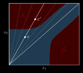
(a) Stopping region in $\operatorname{\mathcal{X}}$

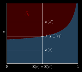
(b) Stopping region through $(\alpha,\Xi)$

Let us first consider three simple examples:

Example 2.1 (1D American put).

It is well known that there exists a boundary $f^{*}$ as a function of time such that

$$\operatorname{\mathcal{S}}_{t}:=\left\{x\in\operatorname{\mathcal{X}}\ :\ x\leq f^{*}(t)\right\}.$$

In this case, stopping is optimal in the state $(t,x)$ if $x\leq f^{*}(t)$, and the indifference points satisfy $x=f^{*}(t)$. In other words, the stopping region is the hypograph of $f^{*}$ and $f^{*}$ is the stopping boundary.

Example 2.2 (Straddle).

A straddle option involves the both the option of selling and buying the underlying asset. The payoff is therefore given by $\varphi(t,s)=e^{-rt}|s-K|^{+}$. As the reward appreciates when the stock moves away from the strike, the stopping region has two boundaries: one lower for selling and one upper for buying, cf. Figure 7. This stopping region is naturally the union of two stopping regions delimited by function graphs:

$$\operatorname{\mathcal{S}}_{t}=\left\{x\in\operatorname{\mathcal{X}}\ :\ x\geq f^{U}(t)\text{ or }x\leq f^{L}(t)\right\}=\left\{x\in\operatorname{\mathcal{X}}\ :\ x\geq f^{U}(t)\right\}\cup\left\{x\in\operatorname{\mathcal{X}}\ :\ x\leq f^{L}(t)\right\},$$

where $f^{L},f^{U}:\operatorname{\mathcal{T}}^{\circ}\to[0,\infty]$ are the lower and upper boundaries, respectively. Although this does not directly fit our main assumption, which assumes a single boundary, this more general case is a natural generalization, cf. Remark 2.2.

In both of the preceding examples, the boundary is described by graphs in the problem’s natural coordinates. Even if this is not the case, it is often possible to construct a coordinate system in which the graph representation holds.

Example 2.3 (Max-call option).

In the financial problem of an American max-call option with two stocks and a given strike $K$, we have $\varphi(t,x)=(\max\{x_{1},x_{2}\}-K)^{+}$ for $x=(x_{1},x_{2})\in\operatorname{\mathcal{X}}$. With Markovian dynamics, the state space is $\operatorname{\mathcal{X}}=\operatorname{\mathbb{R}}_{+}^{2}$. The stopping region is illustrated in Figure 1(b), and the coorindates $(\alpha,\Xi)$ from Theorem 4.1 are $\alpha=\max\{x_{1},x_{2}\}$ and $\Xi=x/\max\{x_{1},x_{2}\}$. ∎

With these examples in mind, we formulate our main assumption: that a stopping boundary exists as a function graph (or union thereof), at least in some coordinates. In Theorem 4.1 below, we verify this assumption for a large class of options, under mild natural structural conditions. More examples are provided in Section 4.

Although the description of the following assumption is technical, its interpretation is quite natural. In words, we assume that there exists a stopping boundary that can be characterized as the graph of some function $f^{*}$ in the appropriate coordinates $(\alpha,\Xi)$. In the applications, the choice of these functions is natural as discussed in Example 2.3 above, and in Section 4.

Assumption 2.1.

(Existence of a stopping boundary) There exist measurable functions

$$\alpha:\operatorname{\mathcal{X}}\to\operatorname{\mathbb{R}}_{+},\quad\Xi:\operatorname{\mathcal{X}}\to\Xi(\operatorname{\mathcal{X}}),\quad f^{*}:\operatorname{\mathcal{T}}^{\circ}\times\ \Xi(\operatorname{\mathcal{X}})\to[0,\infty],$$

and $\eta\in\{-1,+1\}$, so that the map $x\in\operatorname{\mathcal{X}}\mapsto(\alpha(x),\Xi(x))\in\operatorname{\mathbb{R}}_{+}\times\ \Xi(\operatorname{\mathcal{X}})$ is a homeomorphism (i.e., one-to-one, onto, continuous with a continuous inverse) and for every $t\in\operatorname{\mathcal{T}}^{\circ}$,

$$\operatorname{\mathcal{S}}_{t}=\{x\in\operatorname{\mathcal{X}}\ :\ \eta\left(f^{*}(t,\Xi(x))-\alpha(x)\right)\leq 0\}.$$ (2.4)

The parameter $\eta$ determines whether the stopping region is an epigraph or a hypograph of $f^{*}$. In the financial applications, typically $\eta=1$ corresponds to a call type option and the stopping region is an epigraph. While $\eta=-1$ is related to put options.

The surjectivity of $\alpha$ ensures that this characterization is non-trivial, and it additionally implies that for every $c>0$, the point corresponding to the pair $(f^{*}(t,\Xi(x))+\eta c,\Xi(x))$ is in the stopping region $\operatorname{\mathcal{S}}_{t}$, and respectively, to the pair $(f^{*}(t,\Xi(x))-\eta c,\Xi(x))$ is not in $\operatorname{\mathcal{S}}_{t}$. Therefore, the graph of $f^{*}$ in the coordinates $(\alpha(x),\Xi(x))$ given by

$$\{x\in\operatorname{\mathcal{X}}:\alpha(x)=f^{*}(t,\Xi(x))\},$$

is included in the boundary of $\operatorname{\mathcal{S}}_{t}$. In fact, in all examples it separates the stopping and continuation regions. Thus, we call $f^{*}$ the optimal stopping boundary.

Example 2.4 (Example 2.3 continued).

In Theorem 4.1, we show that there exists a stopping boundary $f^{*}$ such that the triplet $(\alpha,\Xi,f^{*})$ with

$$\alpha(x)=\max\{x_{1},x_{2}\},\qquad\Xi(x)=\frac{x}{\alpha(x)},\qquad\eta=1,$$

satisfies the above assumption. Figures 8, 9, 10 below provide examples of these regions. In our numerical approach, the latent variable $\Xi(x)$ is the input to the network approximating the stopping boundary. As $\Xi(x)=\Xi(\gamma x)$ for all $x\in\operatorname{\mathbb{R}}_{+}^{2},$ $\gamma>0$, every ray emanating from the origin is mapped to a single point by the map $\Xi$, and the threshold $f^{*}(t,\Xi(x))$ separates the stopping and continuation regions on this ray. ∎

Remark 2.2.

In the theoretical analysis, we assume that there is a single graph that separates the stopping and continuation region.

More generally, like in the case of Example 2.2, there may be multiple boundaries or other structures. The algorithm we present naturally extends to stopping regions that are unions or intersections of regions delimited by a single graph. This is achieved in the implementation by ‘or’ and ‘and’ operations for the respective set operations.

We thus emphasize that the algorithm in Section 3 has considerably flexibility. ∎

2.3 Value function structure

To obtain some regularity of the value function and the stopping regions, we make the following mild assumption satisfied in all applications. Recall that $\operatorname{\mathcal{L}}_{a}$ is defined in (2.2).

Assumption 2.3.

(Growth and continuity) There exists $a>0$, such that for every $t\in\operatorname{\mathcal{T}}$, $\varphi(t,\cdot)\in\operatorname{\mathcal{L}}_{a}$. Moreover, for every $\phi\in\operatorname{\mathcal{L}}_{a}$, $t<\bar{t}\in\operatorname{\mathcal{T}}$, $v_{\phi}(t,\cdot,\bar{t})\in\operatorname{\mathcal{L}}_{a}$, where

$$v_{\phi}(t,x,\bar{t}):=\operatorname{\mathbb{E}}[\phi(X_{\bar{t}})\mid X_{t}=x],\qquad x\in\operatorname{\mathcal{X}}.$$

The above assumed continuity essentially follows form the continuous dependence of the distribution of the state on its initial value, and it is always satisfied in all our applications.

The following are direct consequences.

Proposition 2.4.

Under the growth and continuity Assumption 2.3, for each $t\in\operatorname{\mathcal{T}}$, the value function $v(t,\cdot)\in\operatorname{\mathcal{L}}_{a}$, and the stopping region $\operatorname{\mathcal{S}}_{t}$ is a relatively closed subset of $\operatorname{\mathcal{X}}$.

Proof.

To prove the first statement, we use backward induction in time $t_{0}<t_{1}<\ldots<t_{n}=T$. First observe that by Assumption 2.3, $v(T,\cdot)=\varphi(T,\cdot)\in\operatorname{\mathcal{L}}_{a}$. For the induction hypothesis, suppose that $v(t_{k+1},\cdot)\in\operatorname{\mathcal{L}}_{a}$ for some $t_{k+1}\in\operatorname{\mathcal{T}}$. By dynamic programming,

$$v(t_{k},x)=\max\left\{\varphi(t_{k},x),\ c(t_{k},x)\right\},\qquad\text{where}\qquad c(t_{k},x):=\operatorname{\mathbb{E}}[v(t_{k+1},X_{t_{k+1}})\mid X_{t}=x].$$

As $v(t_{k+1},\cdot)$ is assumed to be in $\operatorname{\mathcal{L}}_{a}$, Assumption 2.3 implies that $c(t_{k},x)$ is also in $\operatorname{\mathcal{L}}_{a}$. Since the space $\operatorname{\mathcal{L}}_{a}$ is closed under maximization, the above equation implies that $v(t_{k},\cdot)\in\operatorname{\mathcal{L}}_{a}$. Hence, $v(t,\cdot)\in\operatorname{\mathcal{L}}_{a}$ for every $t\in\operatorname{\mathcal{T}}$, and in particular, it is continuous.

The stopping region $\operatorname{\mathcal{S}}_{t}$ is the zero level set of $v(t,\cdot)-\varphi(t,\cdot)$ which is shown to be continuous. Hence, it is relatively closed in $\operatorname{\mathcal{X}}$. ∎

As an immediate consequence of the above assumption, we can restrict the maximization in (2.1) to stopping times given by stopping boundaries. For future reference, we record this fact. Let $\operatorname{\mathfrak{F}}$ be the set of all measurable functions $f:\operatorname{\mathcal{T}}^{\circ}\times\ \Xi(\operatorname{\mathcal{X}})\to[0,\infty]$. For $f\in\operatorname{\mathfrak{F}}$, the corresponding stopping time is given by,

$$\tau_{f}:=\min\left\{u\in\operatorname{\mathcal{T}}\ :\ \eta\left(f(u,\Xi(X_{u}))-\alpha(X_{u})\right)\leq 0\ \ \text{or}\ \ u=T\right\}\in\vartheta.$$

Lemma 2.5.

Under the growth and continuity Assumption 2.3, and the existence of a stopping boundary Assumption 2.1,

$$\sup_{\tau\in\vartheta}v(\tau)=\sup_{f\in\operatorname{\mathfrak{F}}}v(\tau_{f}).$$

Proof.

As $\tau_{f}\in\vartheta$, we have $\sup_{\tau\in\vartheta}v(\tau)\geq v(\tau_{f})$ for all $f\in\operatorname{\mathfrak{F}}$. Let $f^{*}$ be as in Assumption 2.1. Then, for $u\in\operatorname{\mathcal{T}}$, we have $X_{u}\in\operatorname{\mathcal{S}}_{u}$ if and only if, either $\eta\left(f^{*}(u,\Xi(X_{u}))-\alpha(X_{u})\right)\leq 0$, or $u=T$. Therefore, $\tau_{f^{*}}$ is equal to the optimal hitting time $\tau^{*}$ defined in (2.3). These imply that $\sup_{\tau\in\vartheta}v(\tau)\geq\sup_{f\in\operatorname{\mathfrak{F}}}v(\tau_{f})\geq v(\tau_{f^{*}})=v(\tau^{*})=\sup_{\tau\in\vartheta}v(\tau)$. ∎

3 The Algorithm

Our goal is to construct an efficient algorithm for the calculation of the interpretable stopping decisions based on boundaries approximated by artificial neural networks. We train the networks by the deep empirical risk minimization algorithm proposed by Weinan E, Jiequn Han, and Arnulf Jentzen [32, 33].

This method approximates the expected value of a reward function by Monte-Carlo simulations and optimizes it by stochastic gradient ascent. For the problem of optimal stopping, the natural choice for the reward function is $\varphi(\tau_{\theta},X_{\tau_{\theta}})$. However, the map $\theta\mapsto\tau_{\theta}$ is piece-wise constant, making optimization by gradient ascent impossible. Therefore, we replace the hitting times by stopping probabilities based on fuzzy boundaries that are also used in some problems of solidification [12, 27, 50, 53].

3.1 Fuzzy Stopping Boundary

Let $\eta\in\{-1,1\}$ be as in Assumption 2.1. For $f\in\operatorname{\mathfrak{F}}$, set

$$d(t,x;f):=\eta\left(f(t,\Xi(x))-\alpha(x)\right),\qquad t\in\operatorname{\mathcal{T}}^{\circ},\ x\in\operatorname{\mathcal{X}}.$$

In the original problem, once a boundary $f$ is chosen, we stop the process only when $d(t,X_{t};f)\leq 0$. As training is not possible with this sharp “stop-or-continue” rule, we introduce the fuzzy boundaries. Namely, we fix a tuning parameter $\epsilon>0$, and at time $t\in\operatorname{\mathcal{T}}^{\circ}$, define

$$\operatorname{\mathfrak{B}}_{t}^{\epsilon}(f):=\{x\in\operatorname{\mathcal{X}}\ :\ |d(t,x;f)|<\epsilon\}$$

be the fuzzy region.

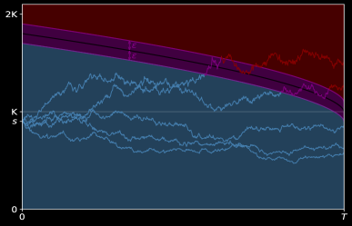
Figure 2: Fuzzy region of an American call (in purple) connecting the stopping region (in red) to the continuation region (in blue).

An illustration of the fuzzy region is given in Figure 2 for an American call option. If the state is not in $\operatorname{\mathfrak{B}}_{t}^{\epsilon}(f)$, we continue or stop, as before, with probability one. But if we are in the fuzzy region, we stop with probability $p_{t}(X_{t},f)$, where

$$p_{t}(x,f):=\left(\frac{\epsilon-d(t,x,f)}{2\epsilon}\right)^{+}\wedge 1,\qquad t\in\operatorname{\mathcal{T}}^{\circ},\ f\in\operatorname{\mathfrak{F}},\ x\in\operatorname{\mathcal{X}}.$$

At maturity, we stop at all states, or equivalently, we set $p_{T}(\cdot,f)\equiv 1$. Precisely, $p_{t}(X_{t},f)$ is the probability of stopping at time $t\in\operatorname{\mathcal{T}}$, conditioned on the event that the process is not stopped prior to $t$. The relaxed control problem is then defined using the reward function given by

$$\operatorname{\mathcal{R}}_{\epsilon}(X,f):=\sum_{t\in\operatorname{\mathcal{T}}}\ p_{t}(X_{t},f)\ b_{t}(X,f)\ \varphi(t,X_{t}),$$ (3.1)

where $b_{t}(X,f)$ is the probability of not stopping strictly before time $t$ and it is obtained as the solution of the following difference equations,

$$b_{t+1}(X,f)=b_{t}(X,f)(1-p_{t}(X_{t},f)),\qquad t\in\operatorname{\mathcal{T}}^{\circ},$$

with $b_{0}(X,f)=1$. In other words, $b_{t}(X,f)$ is the unused stopping-budget remaining. The process $b_{t}(X,f)$ is non-increasing in time and takes values in $[0,1]$. Connection between $\operatorname{\mathbb{E}}[\operatorname{\mathcal{R}}_{\epsilon}(X,f)]$ and $v(\tau_{f})$ is discussed in Appendix B.

We refer to [44] for a different exposition of this relaxation.

3.2 Deep ERM

In this method, we approximate the stopping boundary by a set of deep neural networks that we abstractly parameterize by $\theta$ taking values in a finite-dimensional space $\Theta$ as follows:

$$\operatorname{\mathfrak{N}}=\left\{\ g(\cdot;\theta):\operatorname{\mathcal{T}}^{\circ}\times\ \Xi(\operatorname{\mathcal{X}})\to\operatorname{\mathbb{R}}_{+}\ :\ \theta\in\Theta\ \right\}\subset\operatorname{\mathfrak{F}}.$$

Let $\tau_{\theta}=\tau_{g(\cdot;\theta)}$ be the hitting time corresponding to the stopping boundary $g(\cdot;\theta)$. The following is the pseudocode of the deep empirical risk minimization based on the fuzzy stopping boundary.

1. Initialize $\theta\in\Theta$.

2. Simulate independent state trajectories, $\{X^{(1)},\ldots,X^{(B)}\}$, where $B$ is the batch size.

3. Compute the empirical reward function:

   $$R_{\epsilon}(\theta):=\frac{1}{B}\ \sum_{i=1}^{B}\ \operatorname{\mathcal{R}}_{\epsilon}(X^{(i)},g(\cdot;\theta)),$$

   where $\operatorname{\mathcal{R}}_{\epsilon}(X,f)$ is as in (3.1). A modification $\operatorname{\mathcal{R}}_{\epsilon,\lambda}$, given in (4.4), allows for importance sampling discussed in Section 4.1 below.

4. Optimize and update by stochastic gradient ascent with the learning rate process $\zeta$:

   $$\theta\,\leftarrow\,\theta+\zeta\nabla_{\theta}R_{\epsilon}(\theta).$$

5. Stop after $M$ number of iterations.

6. Compute the initial price given by the training network, using $J$ many Monte-Carlo simulations with a sharp boundary.

A formal discussion of the algorithm is given in the next subsection. In Appendix C, we also provide more details of the above algorithm for the benefit of readers interested in the implementation. [28] proposes a similar approach by assuming that the stopping region has a finite dimensional representation without a formal justification. Also, Chapter 8.2 of [30] discusses a general approximation for the value calculation by parametrizing the stopping times. In our approach we approximate the stopping boundary directly.

3.3 Discussion

The general theory of stochastic gradient ascent [45] implies that the above algorithm constructs an approximation of

$$\theta_{\epsilon}^{*}\in\arg\max_{\theta\in\Theta}\ \operatorname{\mathbb{E}}\left[\operatorname{\mathcal{R}}_{\epsilon}(X,g(\cdot;\theta))\right].$$

In the context of optimal stopping, [11] also provides rates of convergence. Moreover, in Lemma B.1 below, we show that for each $\theta\in\Theta$,

$$\lim_{\epsilon\downarrow 0}\ \operatorname{\mathbb{E}}[\operatorname{\mathcal{R}}_{\epsilon}(X,g(\cdot;\theta))]=\operatorname{\mathbb{E}}[\varphi(\tau_{\theta},X_{\tau_{\theta}})]=v(\tau_{\theta}).$$

Therefore,

$$\operatorname{\mathbb{E}}\left[\operatorname{\mathcal{R}}_{\epsilon}(X,g(\cdot;\theta_{\epsilon}^{*}))\right]=\sup_{\theta\in\Theta}\ \operatorname{\mathbb{E}}\left[\operatorname{\mathcal{R}}_{\epsilon}(X,g(\cdot;\theta))\right]\approx\sup_{\theta\in\Theta}\ v(\tau_{\theta}).$$

Also, by the celebrated universal approximation theorem [21, 34], continuous stopping boundaries are well approximated by the hypothesis class $\operatorname{\mathfrak{N}}$, and in all our applications the optimal stopping boundaries are continuous. Thus, in view of this approximation capability of $\operatorname{\mathfrak{N}}$ and Lemma 2.5, we formally have

$$\operatorname{\mathbb{E}}\left[\operatorname{\mathcal{R}}_{\epsilon}(X,g(\cdot;\theta_{\epsilon}^{*}))\right]=\sup_{\theta\in\Theta}\ \operatorname{\mathbb{E}}\left[\operatorname{\mathcal{R}}_{\epsilon}(X,g(\cdot;\theta))\right]\approx\sup_{\theta\in\Theta}\ v(\tau_{\theta})\approx\sup_{f\in\operatorname{\mathfrak{F}}}\ v(\tau_{f})=\sup_{\tau\in\vartheta}\ v(\tau).$$

Hence, the above algorithm constructs an artificial neural network with an asymptotic performance formally close to the optimal value, justifying the algorithm. However, there are several technical issues in front a rigorous statement and we postpone this convergence analysis to another manuscript [51].

4 Financial Examples

We numerically study several American or Bermudan options to illustrate and also assess the proposed algorithm. In these applications, $\operatorname{\mathbb{Q}}$ is a risk-neutral measure and the Markov state process $X=(S,Y,Z)$ has three components: $S$ is the prices of the underlying stocks possibly including the past values to make it Markov, a factor process $Y$ used in models like Heston, and a functional $Z$ of the stock process, making the pay-off of a path-dependent option a function of the current value of $X$. Typical examples of $Z$ are the running maximum or minimum in look-back options, and the average stock price for the Asian options. Depending on the model and the option, $Y$, $Z$, or neither may be present.

In our examples, the pay-off function always has the following form:

$$\varphi(t,x)=e^{-rt}\left(\eta(\alpha(s,z)-\beta(s,z)-K)\right)^{+},\qquad t\in\operatorname{\mathcal{T}},\ x=(s,y,z)\in\operatorname{\mathcal{X}},$$ (4.1)

where $\alpha>0,\beta\geq 0$ are positively homogenous of degree one, and the parameter $\eta\in\{-1,+1\}$ determines the option type: $\eta=1$ is a call and $\eta=-1$ is a put. The choice of $\alpha$ and $\beta$ may not be unique, and we would choose $\beta\equiv 0$ when possible. It is clear that $\varphi$ grows linearly. Additionally, in all our examples, the stock price distribution depends smoothly on the initial data. Hence, the growth and continuity Assumption 2.3 holds with $a=1$.

The following stopping boundary result is proven in the Appendix. For max-call options a similar result is proved in Proposition A.5 in [14], and for look-back options in [22].

Theorem 4.1.

Suppose that in (4.1), $\alpha:\operatorname{\mathcal{X}}\to\operatorname{\mathbb{R}}_{+}$, $\beta:\operatorname{\mathcal{X}}\to[0,\infty)$ are positively homogenous of degree one, and that $X$ scales linearly in the initial values $S_{t}=s,Z_{t}=z$, i.e., for $x=(s,y,z)$, $\gamma>0$, and a bounded, continuous, integrable function $\phi$, the following holds:

$$\operatorname{\mathbb{E}}\left[\phi(u,X_{u})\mid X_{t}=(\gamma s,y,\gamma z)\right]=\operatorname{\mathbb{E}}\left[\phi(u,\gamma X_{u})\mid X_{t}=(s,y,z)\right].$$

Further assume that the growth and continuity Assumption 2.3 holds, and the price of the European option is strictly positive for all $t<T$. Then, the existence of a stopping boundary Assumption 2.1 is satisfied with $\alpha$ as in (4.1),

$$\Xi(s,y,z)=\left(\frac{s}{\alpha(s,z)}\,,\,y\,,\,\frac{z}{\alpha(s,z)}\right),$$ (4.2)

and

$$f^{*}(t,\xi):=\left\{\begin{array}[]{ll}\sup\left\{\alpha(s,z)\ :\ x\in\operatorname{\mathcal{S}}_{t}\ \ \text{s.t.}\ \ \Xi(x)=\xi\right\},&\text{if}\ \ \eta=-1,\\ \,\inf\left\{\alpha(s,z)\ :\ x\in\operatorname{\mathcal{S}}_{t}\ \ \text{s.t.}\ \ \Xi(x)=\xi\right\},&\text{if}\ \ \eta=1,\end{array}\right.$$ (4.3)

where we use the convention that the sup over the empty set is zero and inf is infinity.

The positivity of the European price ensures that on stopping regions $\varphi>0$.

4.1 Importance sampling

To effectively train the network $g(\cdot;\theta)$ by deep ERM, it is crucial that the simulated paths $X_{t}$ hit the fuzzy boundary $\operatorname{\mathfrak{B}}_{t}^{\epsilon}(g(\cdot;\theta))$ frequently enough for each exercise date. We achieve this by importance sampling that we now outline.

In all our examples, $S$ evolves according to a stochastic differential equation,

$$dS_{t}=S_{t}\left(\mu_{t}dt+\sigma_{t}dW_{t}\right),\quad s_{0}\in\operatorname{\mathbb{R}}^{d},$$

where the processes $\mu\in\operatorname{\mathbb{R}}^{d}$, $\sigma\in\operatorname{\mathbb{R}}^{d\times d}$ may depend on $t,S_{t}$ and other exogenous factors. For $\lambda=(\lambda_{1},\dots,\lambda_{d})\in\operatorname{\mathbb{R}}^{d}$, let $\operatorname{\mathbb{Q}}_{\lambda}$ be the measure obtained by the Girsanov transformation so that $W_{t}^{\lambda}:=W_{t}+\lambda t$ is a $\operatorname{\mathbb{Q}}_{\lambda}$ Brownian motion. Hence, under $\operatorname{\mathbb{Q}}_{\lambda}$,

$$dS_{t}=S_{t}\left([\mu_{t}-\sigma_{t}\lambda]dt+\sigma_{t}dW^{\lambda}_{t}\right).$$

We then adjust the hitting frequency of the simulated trajectories, by choosing $\lambda$ appropriately, thus allowing for more efficient training. Although in all our experiments we have employed constant $\lambda$, one could also use time dependent ones as well.

However, as the probability measure is modified, we need to account for it in the reward function. This is achieved by the Radon-Nikodym derivative given by,

$$\operatorname{\mathcal{Z}}^{\lambda}_{t}(S):=\frac{d\operatorname{\mathbb{Q}}}{d\operatorname{\mathbb{Q}}_{\lambda}}\big{|}_{\operatorname{\mathcal{F}}_{t}}=\exp(\lambda\cdot W_{t}^{\lambda}-\frac{1}{2}|\lambda|^{2}t).$$

Since $W^{\lambda}$ can be expressed in terms of $S$, the process $\operatorname{\mathcal{Z}}^{\lambda}$ can be viewed as a function of the state process $S$. We then modify the reward function given in (3.1) by,

$$\operatorname{\mathcal{R}}_{\epsilon,\lambda}(X,f):=\sum_{t\in\operatorname{\mathcal{T}}}\ \operatorname{\mathcal{Z}}^{\lambda}_{t}(S)\ p_{t}(X_{t},f)\ b_{t}(X,f)\ \varphi(t,X_{t}).$$ (4.4)

4.2 Network Architecture and Parameters

All our numerical experiments have been carried out with Tensorflow 2.7 on a 2021 Macbook pro with 64GB unified memory and Apple M1 Max chip. The code is implemented in Python and run on CPU (10-core) only. Throughout the examples, we use the same neural network architecture and training parameters, given below:

1. We use only one deep neural network that takes both the time and the state vector as input. Then, the trained boundary is a function of the continuous time variable, delivering smoother dependence on time. This is in contrast to majority of previous studies that use one deep neural network for each time in the discrete set $\operatorname{\mathcal{T}}$.

2. The single feedforward neural network that we employ consists of $2$ hidden layers with leaky rectified linear unit (Leaky ReLU) activation function. Each layer has $20+\bar{d}$ many nodes where $\bar{d}$ is the dimension of the latent space $\Xi(\operatorname{\mathcal{X}})$. The output layer uses the standard rectified linear unit (ReLU) activation. An important parameter is the bias $\theta_{0}\in\operatorname{\mathbb{R}}_{+}$ in the output layer that sets an initial boundary level. Namely, the output function $g$ is given by,

$$g(t,\xi;\theta_{1},\theta_{0},\theta_{in})=\left(\theta_{1}\cdot g_{in}(t,\xi;\theta_{in})+\theta_{0}\right)^{+},$$

where $g_{in}(t,\xi;\theta_{in})\in\operatorname{\mathbb{R}}^{20+\bar{d}}$ is the value of the neural network before entering the output layer, with parameters $\theta_{in}$. In our experiments, we have observed that the algorithm is not sensitive to the initial bias $\theta_{0}$, as long as it is set to a reasonable value. For example, for options with a given strike $K$, we choose $\theta_{0}=\frac{3K}{2}$, $\theta_{0}=\frac{K}{2}$ for calls and puts, respectively.

3. We set the number of stochastic gradient iterations to $M=3,000$ with a fixed simulation batch size of $B=512$.

4. The learning rate process $\zeta$ is taken from the Adam optimizer [36].

5. The fuzzy region width $\epsilon$ is chosen to be the strike $K$ times the standard deviation of the increments of $\alpha(X)$. While the strike $K$ adjusts to the scale of the payoff, the second term reflects the typical variation of the process $\alpha(X)$ between exercise dates.

5. After the training is completed, the initial price is computed using the sharp boundary and $J=2^{22}=4,194,304$ many Monte Carlo simulations.

4.3 One-dimensional Put Option

As an initial study, we consider an at the money Bermudan put option in the Black Scholes model. Hence, $\varphi(t,s)=e^{-rt}(K-s)^{+}$, $\eta=-1$, and $X_{t}=S_{t}$ with $\operatorname{\mathcal{X}}=\operatorname{\mathbb{R}}_{+}$.

We take the same model and parameters as in Section 4.3.1.2 of [9]. Namely, $S_{t}$ follows the Black-Scholes model with parameters

$$s_{0}=K=40,\ r=6\%,\ \sigma=40\%,\ T=1,\ n=50,$$ (4.5)

so that $\operatorname{\mathcal{T}}=\{0,\frac{1}{50},\ldots,1\}$. For efficient training, we want the the stock price to reach low values to cross the boundary. Towards this goal, we use use importance sampling with $\lambda=0.275$, so that $S$ becomes a super-martingale under $\operatorname{\mathbb{Q}}_{\lambda}$ with $5\%$ negative drift. The fuzzy region width is approximately equal to $\epsilon=K\sigma\sqrt{T/n}$.

It is classical that the existence of a stopping boundary Assumption 2.1 holds with $\alpha(s)=s$ and $\Xi(s)\equiv 0$. Table 1 summarizes the performance values and compares it to the values computed by Becker et.al. [7]. The first column in that table is the average price of ten experiments, and the second column the highest price. In practice, one would of course retain the trained boundary yielding the highest price.

Bermudan with parameters as in (4.5)

Average Price	Highest Price	Runtime	Price in [9]
5.308 (0.003)	5.313 (0.003)	57.9	5.311

Table 1: Bermudan Put Option with $n=50$ in Black-Scholes model. First column is the average of ten experiments with its standard deviation in brackets. The second column is the highest price among the realizations and its standard deviation in brackets. Third column is the average runtime (in seconds) per experiment for the training phase.

Figure 3 displays the initial boundary and the trained one. The optimal boundary, shown in blue, is computed using a finite-difference scheme. Figure 4 is the approximation of the optimal stopping boundary for the American option with same parameters. As the American option does not restrict the trading dates, we use $n=250$. Also, to capture the known singular behavior of the optimal boundary, we use a non-uniform discretization that is finer near maturity.

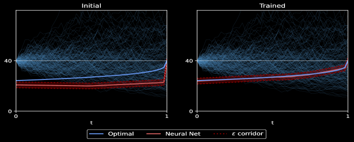
Figure 3: Black-Scholes model with parameters as in (4.5). Blue trajectories are simulated paths.

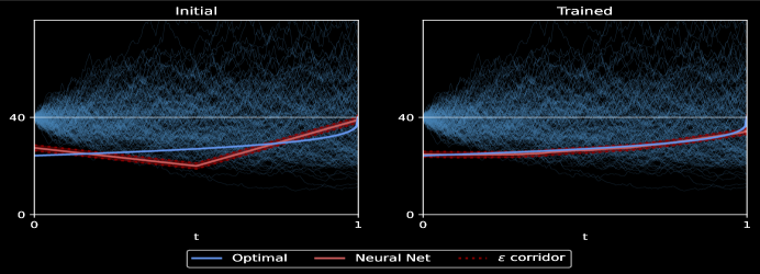
Figure 4: Almost American option in Black-Scholes model with parameters as in (4.5) except $n=250$.

4.4 Put Option in the Heston Model

Consider the Bermudan put option of the Section 4.3 (i.e., $s_{0}=K=40$, $T=1$, $n=50$) but now in the Heston model. Then, under a risk-neutral measure $\operatorname{\mathbb{Q}}$, the stock and factor dynamics are given by,

$$\frac{dS_{t}}{S_{t}} =rdt+\sqrt{Y_{t}}\ dW_{t},$$

$$dY_{t} =(\kappa(\bar{y}-Y_{t})-\gamma_{\operatorname{\mathbb{Q}}}Y_{t})dt+\sigma_{Y}\sqrt{Y_{t}}\ d\tilde{W}_{t},$$

where $W,\tilde{W}$ are Brownian motions with constant correlations $\rho$, and $\gamma_{\operatorname{\mathbb{Q}}}$ is the volatility risk premium related to the risk-neutral measure $\operatorname{\mathbb{Q}}$. We use the parameters

$$r=6\%,\ \kappa=1,\ \sqrt{Y_{0}}=\sqrt{\bar{y}}=40\%,\ \gamma_{\operatorname{\mathbb{Q}}}=0,\ \sigma_{Y}=0.5,\ \rho=-0.5.$$

In particular, the Feller condition $2\kappa\bar{y}\geq\sigma_{Y}^{2}$ is satisfied. To allow for a comparison with results of Section 4.3, we set the initial value and the long term mean $\sqrt{\bar{y}}$ of the stochastic volatility $\sqrt{Y}$ equal to the Black-Scholes volatility $\sigma$ from that section. Moreover, we use importance sampling with the same Girsanov parameter, $\lambda=0.275$. The variance process is simulated using the Milstein scheme [37] with $n^{\prime}=4n=200$ time steps.

In this example, $X=(S,Y)$, $\operatorname{\mathcal{X}}=\operatorname{\mathbb{R}}_{+}^{2}$, $\alpha(x)=s$, $\beta\equiv 0$, and $\Xi(x)=(1,y)$. We simplify and set $\Xi$ to $y$. Figure 5 shows that the stopping boundary is a function of time $t$ and the spot variance $Y_{t}=y$. As $\varphi$ is convex and bounded, the value function $v(t,s,y)$ is non-decreasing in $y$ for all $t\in[0,T]$, cf. [39]. Consequently, the map $y\mapsto f(t,y)$ is non-increasing and the trained neural network $g(\cdot,\cdot;\theta^{M})$ has the same property as seen in Figure 5. Notice also that $y\mapsto f(t,y)$ becomes less steep as $t$ approaches maturity. This is line with the fact that the vega of the option decreases over time prior to the exercise date. Since $s\mapsto v(t,s,y)$ is non-increasing for fixed $(t,y)$, we therefore expect that the rectangle $[0,s]\times[0,y]$ is contained in $\operatorname{\mathcal{S}}_{t}$ whenever $(s,y)\in\operatorname{\mathcal{S}}_{t}$. This is also confirmed in Figure 5.

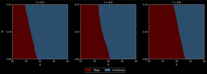
Figure 5: Stopping and continuation regions for a Bermudan put in the Heston model.

Table 2 reports the prices of the claim. Note that the longer runtime compared to Table 1 is due to the thin partition needed to simulate the spot variance process $Y$.

Bermudan Put Option ($n=50$), Heston model

Average Price	Highest Price	Runtime
5.033 (0.003)	5.037 (0.003)	201.0

Table 2: First column is the average of ten experiments with its standard deviation in brackets. Second column is the highest price among the realizations and its standard deviation in brackets. Third column is the average run-time (in seconds) per experiment for the training phase.

Finally, Figure 6 displays a trajectory of $(X,Y)$ together with the trained stopping boundary $g(\cdot;\theta^{M})$. As can be seen, the threshold is typically below the Black-Scholes boundary (red curve) when $Y_{t}$ is above its mean $\bar{y}=0.16$ and vice versa.

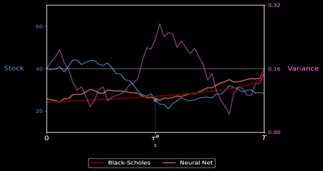
Figure 6: Stock price, variance and threshold process for a Bermudan put in the Heston model.

4.5 Bermudan Straddle

Consider a Bermudan straddle in the Black-Scholes model, that is $\varphi(t,s)=e^{-rt}|s-K|^{+}$, $X_{t}=S_{t}$, and $\operatorname{\mathcal{X}}=\operatorname{\mathbb{R}}_{+}$. As already seen in Example 2.2, the payoff is not of the form (4.1). The purpose of this section is therefore to demonstrate the flexibility of the method. As argued in Example 2.2, there exist two boundaries $f^{U},f^{L}:\operatorname{\mathcal{T}}^{\circ}\to[0,\infty]$ such that $\operatorname{\mathcal{S}}=\operatorname{\mathcal{S}}^{L}\cup\operatorname{\mathcal{S}}^{U},$ where $\operatorname{\mathcal{S}}^{\text{U}}$ (respectively $\operatorname{\mathcal{S}}^{\text{L}}$) is the epigraph of $f^{U}$ (resp. hypograph of $f^{L}$).

We consider the same Black-Scholes parameters as in (4.5), except that the stock has a dividend rate of $\delta=0.06$. This is to prevent that the option is never exercised prior to maturity when the underlying is above the strike, in which case $f^{U}\equiv\infty$. The

In the implementation, we reconfigure the neural network with a two-dimensional output and train the lower and upper boundaries simultaneously. Because of the symmetry of the problem, it is reasonable to make the the underlying process a martingale so as to visit both high and low values. Since $r=\delta=0.06$, the drift is already zero under $\operatorname{\mathbb{Q}}$ so importance sampling is not used in this case. The results are given in Table 3 and the two boundaries illustrated in Figure 7. As can be seen, the neural network can effectively handle multiple boundaries.

Bermudan Straddle $(n=50)$, Black-Scholes model

Average Price	Highest Price	Runtime	LSMC Price
12.080 (0.004)	12.087 (0.004)	24.6	12.018 (0.004)

Table 3: Bermudan at-the-money Straddle with $n=50$ in Black-Scholes model. First column is the average of ten experiments with its standard deviation in brackets. The second column is the highest price among the realizations and its standard deviation in brackets. Third column is the average runtime (in seconds) per experiment for the training phase and fourth column is the price obtained with the Least square Monte Carlo algorithm.

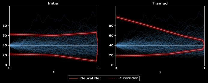
Figure 7: Bermudan straddle ($n=50$) in the Black-Scholes model.

4.6 Bermudan Max-Call

We now apply the deep empirical risk minimization to the classical example of the max-call option on dividend paying stocks as studied in the seminal paper by Broadie & Detemple [14], and also in the book by Detemple [24].

We assume that the stock price process $S_{t}=(S^{(1)}_{t},\ldots,S^{(d)}_{t})\in\operatorname{\mathbb{R}}_{+}^{d}$ is the state process and solves

$$dS^{(i)}_{t}=S^{(i)}_{t}\Big{(}(r-\delta_{i})dt+\sigma_{i}dW^{(i)}_{t}\Big{)},$$

where $\delta_{i}$ is the dividend rate. In this example, the reward function is given by,

$$\varphi(t,s)=e^{-rt}(\alpha(s)-K)^{+},\quad\text{where}\quad\alpha(s)=\max\{s_{1},\ldots,s_{d}\},\qquad s\in\operatorname{\mathbb{R}}_{+}^{d}.$$

Hence, $X=S$, $\operatorname{\mathcal{X}}=\operatorname{\mathbb{R}}_{+}^{d}$, $\eta=1$, and $\beta\equiv 0$. In view of Theorem 4.1, the existence of a stopping boundary Assumption 2.1 holds with $\alpha$ and $\Xi(s)=s/\alpha(s)$. In two dimensions, the stopping regions can be visualized effectively as seen in the Figures 8, 9 reported from [44]. These are stopping regions in two space dimensions obtained with initial data $s_{0}=90$ and $s_{0}=100$ with parameters given in (4.6). Clearly the stopping boundary is independent of the initial condition and the below numerical results verify it. Also they are very similar to those obtained in [14].

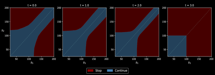
Figure 8: Stopping Boundaries with $s_{0}=90$, $K=100$, $\sigma_{i}=0.2$, $r=0.05$, $\delta_{i}=0.1$, reported from [44].

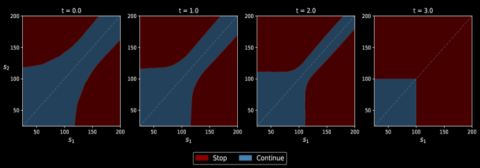
Figure 9: Stopping Boundaries with $s_{0}=100$, $K=100$, $\sigma_{i}=0.2$, $r=0.05$, $\delta_{i}=0.1$, reported from [44].

4.6.1 Symmetric Max-call

As in [7, 9], we use the following parameter set:

$$K=100,\ s_{0}=100,\ \sigma_{i}=0.2,\ r=0.05,\ \delta_{i}=0.1.$$ (4.6)

We take the maturity to be $3$ years and $n=9$. Thus, each time interval corresponds to four months. Numerical experiments for these parameters are reported in the accompanying paper [44]. They compare well to the results obtained in [7, 9].

We also compute the initial price of this max option on $d\in\{2,5,10,20,50\}$ assets. Since we observe that the drift of the maximum stock price process is of order $\ln(d)$, we use important sampling with $\lambda_{i}=(r-\delta_{i}-\mu(d))/\sigma$ and $\mu(d)=-0.01\ln(d)$ to ensure that the maximum stock value does not cross the stopping boundary too soon. Utilizing the fact that the stocks are exchangeable in this example, we order the stock prices $s_{(1)}\geq s_{(2)}\geq\ldots$ and input the second to sixth largest ratios $(\frac{s_{(2)}}{\alpha(s)},\ldots,\frac{s_{(6)}}{\alpha(s)})$ to the neural network (note that the first ratio $\frac{s_{(1)}}{\alpha(s)}\equiv 1$ and is therefore omitted).

Table 4 summarizes the results. Despite a low cutoff, the obtained prices are close or above the benchmark. Moreover, the runtime remains moderate as $d$ increases. The case $d=5$ is a classical example first introduced by Broadie and Glasserman [15] and well-studied later in the literature. Table 4 also contains the tight confidence intervals, obtained in [1], [13], and [7] using a primal-dual method.

Max-call option with parameters in (4.6) and $s_{0}=100$

$d$	Average Price	Highest Price	Runtime	Price in [9]	Confidence Intervals
2	13.883 (0.009)	13.898 (0.008)	29.1	13.901	[13.892, 13.934]   ([1])
5	26.130 (0.010)	26.151 (0.009)	31.8	26.147	[26.115, 26.164]   ([13])
10	38.336 (0.015)	38.355 (0.011)	33.1	38.272	[38.300, 38.367]   ([7])
20	51.728 (0.018)	51.753 (0.011)	36.0	51.572	[51.549, 51.803]   ([7])
50	69.860 (0.012)	69.881 (0.011)	43.5	69.572	[69.560, 69.945]   ([7])

Table 4: Max Option on $d\in\{5,10,20,50\}$ symmetric assets. The second column is the average of ten experiments with its standard deviation in brackets. The third column is the highest price among the realizations and its standard deviation in brackets. The fourth column is the average runtime (in seconds) per experiment for the training phase.

4.6.2 Asymmetric Max-call

We next investigate the Bermudan max option with asymmetric assets. We consider two stocks with same volatility $\sigma$ but different dividend rates. We use the same parameters for $K,r,\sigma$ as in the previous subsection, and $s_{0}=100$, $\delta=(5\%,15\%)$.

We choose the parameter $\lambda$ in the Girsanov theorem, so as to make the assets symmetric under an equivalent measure. More precisely, we choose $\lambda=[(r+\mu(2))(1,1)-\delta]/{\sigma}\in\operatorname{\mathbb{R}}^{2}$ so that both assets have the same drift $\mu(2)\in\operatorname{\mathbb{R}}$ under $\operatorname{\mathbb{Q}}_{\lambda}$, and $\mu(2)=-0.01\ln(2)$ is as in the previous subsection. The asymmetry is then captured by the Radon-Nikodym derivative appearing in the reward function.

The average and highest price after $10$ realizations are given in Table 5. The last column is a benchmark price obtained from the Least Square Monte Carlo (LSMC) algorithm [40] with $2^{22}$ simulations. As can be seen, our method in average computes a price comparable to the benchmark, but may construct better stopping strategies reported in the second column. Notice also that having different dividends gives a premium over the symmetric case as shown in the first row of Table 4.

Max-call option with asymmetric assets

Average Price	Highest Price	Runtime	LSMC Price
15.551 (0.014)	15.575 (0.011)	30.9	15.558 (0.009)

Table 5: Max Option on $d=2$ asymmetric assets

Figure 10 displays the stopping and continuation region over time. In particular, we clearly see the assymmetry of the problem and the stopping region reflected in the figure. For $i=1,2$, let the the connected components of $\operatorname{\mathcal{S}}_{t}$ be given by, $\operatorname{\mathcal{S}}^{(i)}_{t}:=\left\{s\in\operatorname{\mathcal{S}}_{t}:\alpha(s)=s_{i}\right\}$. In Figure 10, we observe that the light red region $\operatorname{\mathcal{I}}(\operatorname{\mathcal{S}}^{(1)}_{t})$ with $\operatorname{\mathcal{I}}(s_{1},s_{2}):=(s_{2},s_{1})$, is contained in $\operatorname{\mathcal{S}}^{(2)}_{t}$. That is, if it is optimal to stop at $S_{t}=(s_{1},s_{2})$, then the same is true at $\operatorname{\mathcal{I}}(S_{t})=(s_{2},s_{1})$. The structure of the assymmetry is therefore consistent with our expectations.

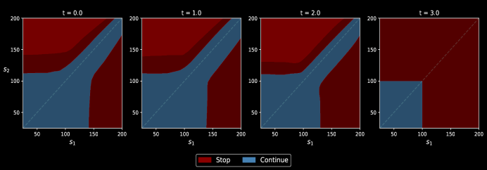
Figure 10: Stopping and continuation regions for a max option with $d=2$ assets and $T=3$. The light red region is the reflection of the lower stopping region $\{s\in\operatorname{\mathcal{S}}_{t}\ :\ s_{1}\geq s_{2}\}$ through the diagonal.

Remark 4.2.

For max-call options on two assets, [28] also use a two-dimensional parametrization of the stopping region given by

$$\operatorname{\mathcal{S}}_{t}\approx\left\{(s_{1},s_{2})\in\operatorname{\mathbb{R}}_{+}^{2}\ :\ \alpha(s)=\max\{s_{1},s_{2}\}\geq\theta_{t}^{1},\ \text{and}\ \ |s_{1}-s_{2}|\geq\theta_{t}^{2}\ \right\}.$$

While the above hypothesis class of regions provides satisfactory numerical results, they are restricted to two dimensions, and only give a simple polygonal approximation of the actual stopping regions that are more complex as can be seen in the Figures 8, 9, 10.

4.6.3 Up-and-Out Max-call

We consider a Bermudan up-and-out max-call option on $d\geq 2$ symmetric assets. That is, the payoff is given by

$$\varphi(X_{t})=(\alpha(S_{t})-K)^{+}\mathds{1}_{\{Z_{t}\leq b\}},\quad X_{t}=(S_{t},Z_{t})\in\operatorname{\mathbb{R}}^{d+1}_{+},\quad(\alpha(s)=\max\{s_{1},\ldots,s_{d}\})\\$$

where $b$ is the barrier and $Z_{t}=\overline{S}_{t}:=\max_{u\in[0,t]}\alpha(S_{u})$ is the running maximum across all assets. We take the parameters from [23], namely

$$K=100,\ b=170,\ s_{0}=100,\ \sigma_{i}=0.2,\ r=0.05,\ \delta_{i}=0,\ T=3,\ N=54.$$

In this example, we set $\Xi(x)=(s/\alpha(s),z)$ instead of $\Xi(x)=x/\alpha(s),\ x=(s,z)$. In other words, the raw running maximum is given to the boundary instead of the ratio $\bar{S}_{t}/\alpha(S_{t})$ to directly compare $\bar{S}_{t}$ with the barrier level. We use the same cutoff (5 assets) and Girsanov parameter as in Figure 4.6.1. The results are reported in Figure 6. As can be seen, the average and highest prices (first two columns) lies within the price intervals from [23] (last column). Notice that the price of the up-and-out max-call option increases slowly with the number of assets ($d$) because the contract becomes more likely to be knocked out. Indeed, the drift of the running maximum process $\bar{S}$ increases with $d$, increasing the probability of hitting the barrier $b$.

Up-and-Out Max-call option with parameters in (4.6) and $s_{0}=100$

$d$	Average Price	Highest Price	Runtime	Price Interval from [23]
4	42.487 (0.010)	43.093 (0.009)	49.2	[41.541, 43.853]
8	50.905 (0.007)	51.379 (0.006)	57.2	[50.252, 52.053]
16	53.650 (0.007)	54.468 (0.006)	62.7	[53.638, 55.094]

Table 6: Up-and-out max-call option on $d\in\{4,8,16\}$ symmetric assets. The second column is the average of ten experiments with its standard deviation in brackets. The third column is the highest price among the realizations and its standard deviation in brackets. The fourth column is the average runtime (in seconds) per experiment for the training phase.

4.7 Look-back Options

Look-back options provides exposure to the minimum or maximum values attained during the tenure of the option. There are several types of look-back options that are commonly traded as summarized in the Table 7. In these examples, when the stock price $S_{t}\in\operatorname{\mathbb{R}}_{+}$ is modeled as a Markov process, then we would have $X=(S,Z)$, where $Z_{t}$ is either the running maximum $\overline{S}_{t}$ or running minimum $\underline{S}_{t}$ given by,

$$\overline{S}_{t}:=\max_{u\in[0,t]}S_{u},\qquad\underline{S}_{t}:=\min_{u\in[0,t]}S_{u}.$$

Option	$e^{rt}\varphi(t,X_{t})$	$\eta$	$\alpha(s,z)$	$\beta(s,z)$
Fixed Strike Call	$(\overline{S}_{t}-K)^{+}$	$1$	$z$	$0$
Fixed Strike Put	$(K-\underline{S}_{t})^{+}$	$-1$	$z$	$0$
Floating Strike Call	$(S_{t}-\gamma\underline{S}_{t})^{+}$	$1$	$s$	$\gamma z$
Floating Strike Put	$(\gamma\overline{S}_{t}-S_{t})^{+}$	$-1$	$s$	$\gamma z$

Table 7: Different Lookback Options.

Clearly, $X=(S,Z)$ is a Markov process with $\operatorname{\mathcal{X}}=\{x=(s,z)\in\operatorname{\mathbb{R}}_{+}^{2}\ |\ 0<s\leq z\}$, when $Z_{t}=\overline{S}_{t}$, or $\operatorname{\mathcal{X}}=\{x=(s,z)\in\operatorname{\mathbb{R}}_{+}^{2}\ |\ 0<z\leq s\}$ when $Z_{t}=\underline{S}_{t}$. The scaling factor $\gamma$ appearing in the payoff of floating strike options is introduced to reduce the price of these otherwise expensive contracts. We therefore choose $\gamma\in[1,\infty)$ and $\gamma\in(0,1]$ for call and put options, respectively. When $\gamma=1$, the floating strike look-back put (call) option delivers precisely the drawdown (drawup) of the stock. We refer the reader to Dai and Kwok [22] for an introduction and discussion of American look-back claims.

4.7.1 Fixed strike call

Although our setting covers all look-backs, as an example we only consider the fixed strike call. Then, $Z_{t}=\overline{S}_{t}$, $\operatorname{\mathcal{X}}=\{x=(s,z)\in\operatorname{\mathbb{R}}_{+}^{2}\ |\ 0<s\leq z\}$), $\eta=1$, $\alpha(s,z)=z$. By Theorem 4.1, a stopping boundary exist with $\Xi(x)=(s/z,1)$. Notice that $1-(s/z)=(z-s)/z$ is the relative drawdown of the stock. As in [22], we use

$$T=1/2,\quad r=2\%,\quad\delta=4\%,\quad\sigma=30\%.$$ (4.7)

To approximate the American option, we consider a regular partition with $n=200$ many exercise dates. Moreover, we employ an even thinner partition with $n^{\prime}=800$ points for our simulations. This allows us to better approximate the running maximum. Importance sampling is not needed in this example. We visualize the the stopping region in the $(s,y)$ plane, similar to Fig. 3 in [22], where the authors use a finite difference scheme to compute the initial price.

Average Price	Highest Price	Runtime	European Price	Upper Bound
16.827 (0.008)	16.844 (0.007)	216.7	16.808	16.979

Table 8: American look-back call with parameters in (4.7) and $K=100$.

Table 8 summarizes the result for $s_{0}=K=100$. First column in that table is the average of ten experiments with the standard deviation in brackets. The second column is the highest price among the realizations and its standard deviation in brackets. The third column is the average runtime (in seconds) per experiment for the training phase.

The last column is the upper bound given by the forward value of the European price. The European price, denoted by $v_{e}$ provides a lower bound on the American price. The last column is the forward value of European price, $e^{rT}v_{e}$, giving an upper bound for the American price. Since here $e^{rT}\approx 1.01$, the American option only offers little premium over its European counterparts. This is nevertheless fortunate from a performance perspective as it gives a tight interval in which the American price must lie (see, e.g., [20]). We indeed obtain prices that are within the bounds.

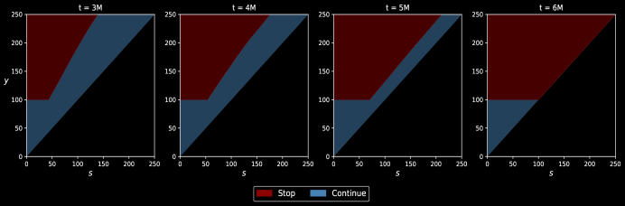
Figure 11: Stopping boundaries for a look-back call with parameters in (4.7) and $K=100$.

We display the stopping and continuation region in Figure 11. Obtaining an overall accurate boundary turns out to be challenging, as visiting all the pairs $(s,y)\in\operatorname{\mathcal{X}}$ is difficult, especially when $s\ll y$. We effectively resolve this issue by randomizing $s_{0}\in\operatorname{\mathcal{X}}$ and setting the initial running maximum to $y_{0}=K\vee s_{0}$. As in Fig. $3$ of [22], we observe a flat boundary when $s\ll K$. That is, the neural network correctly set the boundary equal to the strike when the ratio $s/y$ is small, or equivalently, when the relative drawdown is large.

5 Conclusion

We have developed an algorithm for the computation of the “graph-like” stopping boundaries separating the continuation and stopping regions in optimal stopping. While the method at the high-level is empirical risk minimization, a relaxation based on fuzzy boundaries motivated from phase-field models for liquid-to-solid phase transitions is used. Through numerical experiments, the method is shown to be effective in high-dimensions. The method has the potential to incorporate market details like price impact, transaction costs, and market restrictions. It is also possible to apply the technique to other models from financial economics and other obstacle type problems as long as a control representation is available.

Appendix A Proof of Theorem 4.1

We prove the theorem when the parameter $\eta$ in (4.1) is equal to $-1$. The other case of $\eta=1$ is proved mutatis mutandis. We fix $t\in\operatorname{\mathcal{T}}^{\circ}$.

Firstly, it is clear that for $\Xi$ as in (4.2), the map $x=(s,y,z)\mapsto(\alpha(s,z),\Xi(x))$ is a homeomorphism and $\alpha$ is onto.

Recall that $\vartheta$ is the set of all $\operatorname{\mathcal{T}}$-valued stopping times, $\vartheta_{t}=\vartheta\cap[t,T]$, the pay-off $\varphi(t,x)=\varphi(t,s,z)$ is given by (4.1), and the European price, $v_{e}$, is strictly positive. As the European price is equal to price of the stopping time $\tau\equiv T$, $v(t,x)\geq v_{e}>0$. Therefore, the stopping region is characterized by

$$x\in\operatorname{\mathcal{S}}_{t}\quad\Leftrightarrow\quad v(t,x)=\varphi(t,s,z)>0.$$

We start by showing that $\operatorname{\mathcal{S}}_{t}$ is star-shaped around the origin.

Lemma A.1.

If $x=(s,y,z)\in\operatorname{\mathcal{S}}_{t}$, then $(\gamma s,y,\gamma z)\in\operatorname{\mathcal{S}}_{t}$ for every $\gamma\in(0,1]$.

Proof.

Fix $x=(s,y,z)\in\operatorname{\mathcal{S}}_{t}$ and $\gamma\in(0,1]$. Then, by the definition of the stopping region $\operatorname{\mathcal{S}}_{t}$, $v(t,x)=\varphi(t,s,z)>0$. In particular, as $\eta=-1$, $\alpha(s,z)-\beta(s,z)<K$ and therefore,

$$\alpha(\gamma s,\gamma z)-\beta(\gamma s,\gamma z)=\gamma(\alpha(s,z)-\beta(s,z))<\gamma K\leq K.$$

Hence, $\varphi(t,\gamma s,\gamma z)=-(\alpha(\gamma s,\gamma z)-\beta(\gamma s,\gamma z)-K)>0$. Moreover,

$$\operatorname{\mathbb{E}}\left[\varphi(\tau,S_{\tau},Z_{\tau})\mid X_{t}=(\gamma s,y,\gamma z)\right]=\operatorname{\mathbb{E}}\left[\varphi(\tau,\gamma S_{\tau},\gamma Z_{\tau})\mid X_{t}=(s,y,z)\right].$$

for all $t\in\operatorname{\mathcal{T}}^{\circ}$, $x=(s,y,z)$, $\tau\in\vartheta_{t}$, and $\gamma>0$. By (4.1) and the homogeneity of $\alpha$ and $\beta$,

$$\varphi(\tau,\gamma S_{\tau},\gamma Z_{\tau}) =e^{-r\tau}\left(-(\alpha(\gamma S_{\tau},\gamma Z_{\tau})-\beta(\gamma S_{\tau},\gamma Z_{\tau})-K)\right)^{+}$$

$$=e^{-r\tau}\left(-(\gamma\alpha(S_{\tau},Z_{\tau})-\gamma\beta(S_{\tau},Z_{\tau})-K)\right)^{+}$$

$$\leq e^{-r\tau}\gamma\left(-(\alpha(S_{\tau},Z_{\tau})-\beta(S_{\tau},Z_{\tau})-K)\right)^{+}+e^{-r\tau}(1-\gamma)K$$

$$=\gamma\varphi(\tau,S_{\tau},Z_{\tau})+e^{-r\tau}(1-\gamma)K.$$

We combine the above inequalities to arrive at the following:

$$\operatorname{\mathbb{E}}\left[\varphi(\tau,S_{\tau},Z_{\tau})\mid X_{t}=(\gamma s,y,\gamma z)\right] \leq\gamma\operatorname{\mathbb{E}}\left[\varphi(\tau,S_{\tau},Z_{\tau})\mid X_{t}=(s,y,z)\right]+e^{-rt}(\gamma-1)K$$

$$\leq\gamma v(t,x)+e^{-rt}(1-\gamma)K$$

$$=\gamma\varphi(t,x)+e^{-rt}(1-\gamma)K.$$

As $v(t,x)=\varphi(t,s,z)>0$, again by the homogeneity of $\alpha$ and $\beta$,

$$\varphi(t,\gamma s,\gamma z) =v(t,x)$$

$$=\sup_{\tau\in\vartheta_{t}}\operatorname{\mathbb{E}}\left[\varphi(\tau,S_{\tau},Z_{\tau})\mid X_{t}=(\gamma s,y,\gamma z)\right]$$

$$\leq\gamma\varphi(t,s,z)+e^{-rt}(1-\gamma)K$$

$$=e^{-rt}\left(-(\gamma\alpha(s,z)-\gamma\beta(s,z)-\gamma K)\right)+e^{-rt}(1-\gamma)K$$

$$=e^{-rt}\left(-(\alpha(\gamma s,\gamma z)-\beta(\gamma s,\gamma z)-K)\right)$$

$$=\varphi(t,\gamma s,\gamma z).$$

Hence, $(\gamma s,y,\gamma z)\in\operatorname{\mathcal{S}}_{t}$. ∎

Let $f^{*}$ be as in (4.3). It is clear that if $\alpha(\bar{x})>f^{*}(t,\Xi(\bar{x}))$, then $\bar{x}\not\in\operatorname{\mathcal{S}}_{t}$. Now, suppose $\alpha(\bar{x})<f^{*}(t,\Xi(\bar{x}))$ for some $\bar{x}=(\bar{s},\bar{y},\bar{z})$. Then, by the above definition, there exists $x=(s,y,z)\in\operatorname{\mathcal{S}}_{t}$ such that $\alpha(x)\geq\alpha(\bar{x})$ and $\Xi(x)=\Xi(\bar{x})$. By the definition of $\Xi$, we conclude that $y=\bar{y}$ and $(\bar{s},\bar{z})=(\gamma s,\gamma z)$ with $\gamma:=\alpha(\bar{s},\bar{z})/\alpha(s,z)$. Therefore, $(\gamma s,y,\gamma z)=\bar{x}$, and as $\gamma\leq 1$, by the above lemma $\bar{x}\in\operatorname{\mathcal{S}}_{t}$. Summarizing, we have shown that

$$\{\alpha<f^{*}\}\subset\operatorname{\mathcal{S}}_{t},\quad\text{and}\quad\{\alpha>f^{*}\}\subset\operatorname{\mathcal{X}}\setminus\operatorname{\mathcal{S}}_{t}.$$

Now suppose that $\alpha(x)=f^{*}(t,\Xi(x))$. Since $\alpha$ is always strictly positive, $f^{*}(t,\Xi(x))>0$. Then, there is a sequence $x_{n}\in\operatorname{\mathcal{S}}_{t}$ with $\Xi(x_{n})=\Xi(x)$ and $\alpha(x_{n})\uparrow f^{*}(t,\Xi(x))=\alpha(x)$. As $(\alpha,\Xi)$ is a homeomorphism, we conclude that $x_{n}$ converges to $x$. Moreover, $\operatorname{\mathcal{S}}_{t}$ is relatively closed in $\operatorname{\mathcal{X}}$, implying that $x\in\operatorname{\mathcal{S}}_{t}$. Hence, $\{\alpha=f^{*}\}\subset\operatorname{\mathcal{S}}_{t}$. Consequently, the triplet $(\alpha,\Xi,f^{*})$ satisfies (2.4), and the existence of a stopping boundary Assumption 2.1 holds.

Appendix B Convergence of $\operatorname{\mathcal{R}}_{\epsilon}$

The following limit result justifies our choice of the reward function $\operatorname{\mathcal{R}}_{\epsilon}$. Further details are given in [51].

Lemma B.1.

Suppose that $X_{t}$ has no atoms for all $t\in(0,T]$ and $x_{0}=X_{0}$ is not on the boundary $f$, i.e., $\alpha(x_{0})\neq f(0,\Xi(x_{0}))$. Then,

$$\lim_{\epsilon\downarrow 0}\ \operatorname{\mathbb{E}}[\operatorname{\mathcal{R}}_{\epsilon}(X,f)]=\operatorname{\mathbb{E}}[\varphi(\tau_{f},X_{\tau_{f}})]=v(\tau_{f}).$$ (B.1)

Proof.

Under above assumptions, for every $t\in\operatorname{\mathcal{T}}^{\circ}$, $d(t,X_{t};f)\neq 0$ with probability one. Then as $\epsilon$ tends to zero, $p_{t}(X_{t},f)$ converges to one if $d(t,X_{t};f)>0$ and respectively, to zero if $d(t,X_{t};f)<0$. Consequently, $b_{t}(X,f)$ converges to one for all $t\leq\tau_{f}$ and respectively, to zero for all $t>\tau_{f}$. These limit statements directly imply that

$$\lim_{\epsilon\downarrow 0}\ \operatorname{\mathcal{R}}_{\epsilon}(X,f)=\varphi(\tau_{f},X_{\tau_{f}}),\qquad\text{a.s.}$$

Moreover, as $b_{t},p_{t}\in[0,1]$, Assumption 2.3 implies that

$$|\operatorname{\mathcal{R}}_{\epsilon}(X,f)|\leq\sum_{t\in\operatorname{\mathcal{T}}}\varphi(t,X_{t})\leq C\sum_{t\in\operatorname{\mathcal{T}}}[1+|X_{t}|^{a}]=:\Phi.$$

Since $\operatorname{\mathcal{T}}$ is finite, by Assumption 2.3, $\Phi$ is integrable. Then, the claimed limit (B.1) follows from the dominated convergence theorem. ∎

Appendix C Algorithm Details

The following is a brief outline of the training part of our algorithm.

Stopping Boundary Training:

1. Initialize $\theta_{0}\in\Theta$

2. For $m=0,\ldots,M-1$

   • Simulate trajectories $(X_{t_{k}}^{j})_{k=0}^{n}$, $\ j=1,\ldots,B$.

   • For $k=0,\ldots,n-1$, $j=1,\ldots$, compute the following quantities:

     $$- d_{k,m,j} =\eta\ \left(g(t_{k},\Xi(X^{j}_{t_{k}});\theta^{m})-\alpha(X^{j}_{t_{k}})\right)$$ signed distances

     $$- p_{k,m,j} =\left(\frac{\epsilon-d_{k,m,j}}{2\epsilon}\right)^{+}\wedge 1\quad\text{(}p_{n,m,j}=1\text{)}$$ stopping probabilities

     $$- b_{k+1,m,j} =b_{k,m,j}(1-p_{k,m,j})\quad\text{(}b_{0,m,j}=1\text{)}$$ stopping budgets

     $$- R_{\epsilon}(\theta_{m}) =\frac{1}{B}\sum_{k=1}^{B}\sum_{k=0}^{n}p_{k,m,j}b_{k,m,j}\varphi(t_{k},X_{t_{k}}^{j})$$ reward function

   • Update: $\theta_{m+1}=\theta_{m}+\zeta_{m}\nabla_{\theta}R_{\epsilon}(\theta_{m})$

3. Return $\theta_{M}$ ∎

In the above algorithm, we fix the width of the fuzzy region $\epsilon>0$, and the learning rate process $\zeta_{m}$ is taken from the Adam optimizer [36]. Also in all financial examples, we use important sampling as discussed in the subsection 4.1. That is, chosen a parameter $\lambda$, we modify the dynamics of the state process $X$ and use it in the simulations. Then, we adjust the reward function as in (4.4). The choice of the tuning parameters $\epsilon$ and $\lambda$ are discussed in the specific examples.

References

- Andersen and Broadie [2004] L. Andersen and M. Broadie. Primal-dual simulation algorithm for pricing multidimensional American options. Management Science, 50(9):1222–1234, 2004.
- Bachouch et al. [2021] A. Bachouch, C. Huré, H. Pham, and N. Langrené. Deep neural networks algorithms for stochastic control problems on finite horizon: Convergence analysis. SIAM Journal on Numerical Analysis, 59(1):525–557, 2021.
- Bachouch et al. [2022] A. Bachouch, C. Huré, N. Langrené, and H. Pham. Deep Neural Networks Algorithms for Stochastic Control Problems on Finite Horizon: Numerical Applications. Methodology and Computing in Applied Probability, 24(1):143–178, March 2022.
- Barles et al. [1993] G. Barles, H. M. Soner, and P. E. Souganidis. Front propagation and phase field theory. SIAM Journal on Control and Optimization, 31(2):439–469, 1993.
- Bayer et al. [2020] C. Bayer, R. Tempone, and S. Wolfers. Pricing American options by exercise rate optimization. Quantitative Finance, 20(11):1749–1760, 2020.
- Bayer et al. [2022] C. Bayer, J. Qiu, and Y. Yao. Pricing options under rough volatility with backward SPDEs. SIAM Journal on Financial Mathematics, 13(1):179–212, 2022.
- Becker et al. [2019] S. Becker, P. Cheridito, and A. Jentzen. Deep optimal stopping. Journal of Machine Learning Research, 20(74):1–25, 2019.
- Becker et al. [2020] S. Becker, P. Cheridito, and A. Jentzen. Pricing and hedging American-style options with deep learning. Journal of Risk and Financial Management, 13(7):158, 2020.
- Becker et al. [2021] S. Becker, P. Cheridito, A. Jentzen, and T. Welti. Solving high-dimensional optimal stopping problems using deep learning. European Journal of Applied Mathematics, 32(3):470–514, 2021.
- Becker et al. [2022] S. Becker, A. Jentzen, M. S. Müller, and P. von Wurstemberger. Learning the random variables in Monte Carlo simulations with stochastic gradient descent: Machine learning for parametric PDEs and financial derivative pricing. arXiv:2202.02717, 2022.
- Belomestny [2011] D. Belomestny. On the rates of convergence of simulation-based optimization algorithms for optimal stopping problems. The Annals of Applied Probability, 21(1):215–239, 2011.
- Boettinger et al. [2002] W. J. Boettinger, J. A. Warren, C. Beckermann, and A. Karma. Phase-field simulation of solidification. Annual Review of Materials Research, 32(1):163–194, 2002.
- Broadie and Cao [2008] M. Broadie and M. Cao. Improved lower and upper bound algorithms for pricing american options by simulation. Quantitative Finance, 8:845–861, 12 2008.
- Broadie and Detemple [1997] M. Broadie and J. Detemple. The valuation of American options on multiple assets. Mathematical Finance, 7:241–286, 1997.
- Broadie and Glasserman [2004] M. Broadie and P. Glasserman. A stochastic mesh method for pricing high-dimensional american options. Journal of Computational Finance, 7:35–72, 2004.
- Buehler et al. [2019a] H. Buehler, L. Gonon, J. Teichmann, and B. Wood. Deep hedging. Quantitative Finance, 19(8):1271–1291, 2019a.
- Buehler et al. [2019b] H. Buehler, L. Gonon, J. Teichmann, B. Wood, and B. Mohan. Deep hedging: hedging derivatives under generic market frictions using reinforcement learning. Technical report, Swiss Finance Institute, 2019b.
- Chevalier et al. [2021] E. Chevalier, S. Pulido, and E. Zúñiga. American options in the Volterra Heston model. arXiv:2103.11734, 2021.
- Ciocan and Mišić [2022] D. Ciocan and V. Mišić. Interpretable optimal stopping. Management Science, 68(3):1616–1638, 2022.
- Conze and Viswanathan [1991] A. Conze and Viswanathan. Path dependent options: The case of lookback options. The Journal of Finance, 46(5):1893–1907, 1991.
- Cybenko [1989] G. V. Cybenko. Approximation by superpositions of a sigmoidal function. Mathematics of Control, Signals and Systems, 2:303–314, 1989.
- Dai and Kwok [2005] M. Dai and Y. K. Kwok. American options with lookback payoff. SIAM Journal on Applied Mathematics, 66(1):206–227, 2005. ISSN 00361399.
- Desai et al. [2012] V. V. Desai, V. F. Farias, and C. C. Moallemi. Pathwise Optimization for Optimal Stopping Problems. Management Science, 58(12):2292–2308, December 2012.
- Detemple [2005] J. Detemple. American-Style Derivatives: Valuation and Computation. Chapman and Hall/CRC Financial Mathematics Series. CRC Press, 2005.
- Fecamp et al. [2020] S. Fecamp, J. Mikael, and X. Warin. Deep learning for discrete-time hedging in incomplete markets. Journal of computational Finance, 2020.
- Fleming and Soner [2006] W. H. Fleming and H. M. Soner. Controlled Markov processes and viscosity solutions, volume 25. Springer Science & Business Media, 2006.
- Fried and Gurtin [1994] E. Fried and M. E. Gurtin. Dynamic solid-solid transitions with phase characterized by an order parameter. Physica D: Nonlinear Phenomena, 72(4):287–308, 1994.
- Garcia [2003] D. Garcia. Convergence and Biases of Monte Carlo estimates of American option prices using a parametric exercise rule. Journal of Economic Dynamics and Control, 27(10):1855–1879, 2003.
- Germain et al. [2021] M. Germain, M. Laurière, H. Pham, and X. Warin. Deepsets and their derivative networks for solving symmetric pdes. arXiv:2103.00838, 2021.
- Glasserman [2004] P. Glasserman. Monte Carlo methods in financial engineering. Springer, 2004.
- Gonon et al. [2019] L. Gonon, J. Muhle-Karbe, and X. Shi. Asset pricing with general transaction costs: Theory and numerics. arXiv:1905.05027, 2019.
- Han and E [2016] J. Han and W. E. Deep learning approximation for stochastic control problems. NIPS, 2016.
- Han et al. [2018] J. Han, A. Jentzen, and W. E. Solving high-dimensional partial differential equations using deep learning. Proceedings of the National Academy of Sciences, 115(34):8505–8510, 2018.
- Hornik [1991] K. Hornik. Approximation capabilities of multilayer feedforward networks. Neural Networks, 4(2):251–257, 1991. ISSN 0893-6080.
- Huré et al. [2019] C. Huré, H. Pham, and X. Warin. Some machine learning schemes for high-dimensional nonlinear PDEs. arXiv:1902.01599, 33, 2019.
- Kingma and Ba [2015] D. Kingma and J. A. Ba. Adam: a method for stochastic optimization. Proceedings of the International Conference on Learning Representations (ICLR), 2015.
- Kloeden and Platen [1992] P. E. Kloeden and E. Platen. Numerical Solution of Stochastic Differential Equations. Springer, 1992.
- Kohler et al. [2008] M. Kohler, A. Krzyżak, and N. Todorovic. Pricing of high-dimensional american options by neural networks. Mathematical Finance, 20, 08 2008.
- Lamberton and Terenzi [2019] D. Lamberton and G. Terenzi. Properties of the American price function in the Heston-type models. arXiv:1904.01653, 2019.
- Longstaff and Schwartz [2001] F. A. Longstaff and E. S. Schwartz. Valuing American options by simulation: a simple least-squares approach. The Review of Financial Studies, 14(1):113–147, 2001.
- Ludkovski [2020] M. Ludkovski. mlosp: Towards a unified implementation of regression Monte Carlo algorithms. arXiv:2012.00729, 2020.
- Osher and Fedkiw [2003] S. Osher and R. Fedkiw. Level Set Methods and Dynamic Implicit Surfaces. Springer, 2003.
- Reppen and Soner [2021] A. M. Reppen and H. M. Soner. Deep empirical risk minimization in finance: an assessment. arXiv:2011.09349, 2021.
- Reppen et al. [2022] A. M. Reppen, H. M. Soner, and V. Tissot-Daguette. Deep stochastic optimization in finance. Digital Finance, pages 1–21, 2022.
- Robbins and Siegmund [1971] H. Robbins and D. Siegmund. A convergence theorem for non negative almost supermartingales and some applications. In Optimizing methods in statistics, pages 233–257. Elsevier, 1971.
- Ruf and Wang [2020a] J. Ruf and W. Wang. Hedging with neural networks. arXiv:2004.08891, 2020a.
- Ruf and Wang [2020b] J. Ruf and W. Wang. Neural networks for option pricing and hedging: a literature review. Journal of Computational Finance, 24(1), 2020b.
- Shkolnikov et al. [2023] M. Shkolnikov, H. M. Soner, and V. Tissot-Daguett. Deep level-set method for stefan problems (with and without surface tension). in preperation, 2023.
- Sirignano and Spiliopoulos [2018] J. Sirignano and K. Spiliopoulos. Dgm: A deep learning algorithm for solving partial differential equations. Journal of Computational Physics, 375:1339–1364, 2018.
- Soner [1995] H. M. Soner. Convergence of the phase-field equations to the Mullins-Sekerka problem with kinetic undercooling. Archive for Rat. Mech. and Analysis, 131(2):139–197, 1995.
- Soner and Tissot-Daguette [2023] H. M. Soner and V. Tissot-Daguette. Stopping times of boundaries: Relaxation and continuity. arXiv:2305.09766, 2023.
- Tsitsiklis and Van Roy [2001] J. N. Tsitsiklis and B. Van Roy. Regression methods for pricing complex American-style options. IEEE Transactions on Neural Networks, 12(4):694–703, 2001.
- Voller and Prakash [1987] V. R. Voller and C. Prakash. A fixed grid numerical modelling methodology for convection-diffusion mushy region phase-change problems. International journal of heat and mass transfer, 30(8):1709–1719, 1987.
- Wang and Perdikaris [2021] S. Wang and P. Perdikaris. Deep learning of free boundary and Stefan problems. Journal of Computational Physics, 428:109914, 2021.
- Warin [2019] X. Warin. Variance optimal hedging with application to electricity markets. Journal of Computational Finance, 23(3):33–59, 2019.