Dynamics of SGD with Stochastic Polyak Stepsizes: Truly Adaptive Variants and Convergence
to Exact Solution
Abstract
Recently Loizou et al. [22], proposed and analyzed stochastic gradient descent (SGD) with stochastic Polyak stepsize (SPS). The proposed SPS comes with strong convergence guarantees and competitive performance; however, it has two main drawbacks when it is used in non-over-parameterized regimes: (i) It requires a priori knowledge of the optimal mini-batch losses, which are not available when the interpolation condition is not satisfied (e.g., regularized objectives), and (ii) it guarantees convergence only to a neighborhood of the solution. In this work, we study the dynamics and the convergence properties of SGD equipped with new variants of the stochastic Polyak stepsize and provide solutions to both drawbacks of the original SPS. We first show that a simple modification of the original SPS that uses lower bounds instead of the optimal function values can directly solve issue (i). On the other hand, solving issue (ii) turns out to be more challenging and leads us to valuable insights into the method’s behavior. We show that if interpolation is not satisfied, the correlation between SPS and stochastic gradients introduces a bias, which effectively distorts the expectation of the gradient signal near minimizers, leading to non-convergence - even if the stepsize is scaled down during training. To fix this issue, we propose DecSPS, a novel modification of SPS, which guarantees convergence to the exact minimizer - without a priori knowledge of the problem parameters. For strongly-convex optimization problems, DecSPS is the first stochastic adaptive optimization method that converges to the exact solution without restrictive assumptions like bounded iterates/gradients.
1 Introduction
We consider the stochastic optimization problem:
| (1) |
where each is convex and lower bounded. We denote by the non-empty set of optimal points of equation (1). We set , and .
In this setting, the algorithm of choice is often Stochastic Gradient Descent (SGD), i.e. , where is the stepsize at iteration , a random subset of datapoints (minibatch) with cardinality sampled independently at each iteration , and is the minibatch gradient.
A careful choice of is crucial for most applications [4, 14]. The simplest option is to pick to be constant over training, with its value inversely proportional to the Lipschitz constant of the gradient. While this choice yields fast convergence to the neighborhood of a minimizer, two main problems arise: (a) the optimal depends on (often unknown) problem parameters — hence often requires heavy tuning ; and (b) it cannot be guaranteed that is reached in the limit [13, 16, 15]. A simple fix for the last problem is to allow polynomially decreasing stepsizes (second option) [23]: this choice for often leads to convergence to , but hurts the overall algorithm speed. The third option, which became very popular with the rise of deep learning, is to implement an adaptive stepsize. These methods do not commit to a fixed schedule, but instead use the optimization statistics (e.g. gradient history, cost history) to tune the value of at each iteration. These stepsizes are known to work very well in deep learning [35], and include Adam [19], Adagrad [11], and RMSprop [29].
Ideally, a theoretically grounded adaptive method should yield fast convergence to without knowledge of problem dependent parameters, such as the gradient Lipshitz constant or the strong convexity constant. As a result, an ideal adaptive method should require very little tuning by the user, while matching the performance of a fine-tuned . However, while in practice this is the case for common adaptive methods such as Adam and AdaGrad, the associated convergence rates often rely on strong assumptions — e.g. that the iterates live on a bounded domain, or that gradients are uniformly bounded in norm [11, 32, 31]. While the above assumptions are valid in the constrained setting, they are problematic for problems defined in the whole .
A promising new direction in the adaptive stepsizes literature is based on the idea of Polyak stepsizes, introduced by [25] in the context of deterministic convex optimization. Recently [22] successfully adapted Polyak stepsizes to the stochastic setting, and provided convergence rates matching fine-tuned SGD — while the algorithm does not require knowledge of the unknown quantities such as the gradient Lipschitz constant. The results especially shines in the overparameterized strongly convex setting, where linear convergence to is shown. This result is especially important since, under the same assumption, no such rate exists for AdaGrad (see e.g. [31] for the latest results) or other adaptive stepsizes. Moreover, the method was shown to work surprisingly well on deep learning problems, without requiring heavy tuning [22].
Even if the stochastic Polyak stepsize (SPS) [22] comes with strong convergence guarantees, it has two main drawbacks when it is used in non-over-parameterized regimes: (i) It requires a priori knowledge of the optimal mini-batch losses, which are not often available for big batch sizes or regularized objectives (see discussion in §1.1) and (ii) it guarantees convergence only to a neighborhood of the solution. In this work, we study the dynamics and the convergence properties of SGD equipped with new variants of SPS for solving general convex optimization problems. Our new proposed variants provide solutions to both drawbacks of the original SPS.
1.1 Background and Technical Preliminaries
Dependency on .
Crucially the algorithm requires knowledge of for every realization of the mini-batch . In the non-regularized overparametrized setting (e.g. neural networks), is often zero for every subset [34]. However, this is not the only setting where is computable: e.g., in the regularized logistic loss with batch size 1, it is possible to recover a cheap closed form expression for each [22]. Unfortunately, if the batch-size is bigger than or the loss becomes more demanding (e.g. cross-entropy), then no such closed-form computation is possible.
Rates and comparison with AdaGrad.
In the convex overparametrized setting (more precisely, under the interpolation condition, i.e. : for all , see also §2), SPSmax enjoys a convergence speed of , without requiring knowledge of the gradient Lipschitz constant or other problem parameters. Recently, [31] showed that the same rate can be achieved for AdaGrad in the same setting. However, there is an important difference: the rate of [31] is technically , where is the problem dimension and is a global bound on the squared distance to the minimizer, which is assumed to be finite. Not only does SPSmax not have this dimension dependency, which dates back to crucial arguments in the AdaGrad literature [11, 21], but also does not require bounded iterates. While this assumption is satisfied in the constrained setting, it has no reason to hold in the unconstrained scenario. Unfortunately, this is a common problem of all AdaGrad variants: with the exception of [33] (which works in a slightly different scenario), no rate can be provided in the stochastic setting without the bounded iterates/gradients [12] assumption — even after assuming strong convexity. However, in the non-interpolated setting, AdaGrad enjoys a convergence guarantee of (with the bounded iterates assumption). A similar rate does not yet exist for SPS, and our work aims at filling this gap.
1.2 Main Contributions
As we already mentioned, in the non-interpolated setting SPSmax has the following issues:
-
Issue (1):
For (minibatch setting), SPSmax requires the exact knowledge of . This is not practical.
-
Issue (2):
SPSmax guarantees convergence to a neighborhood of the solution. It is not clear how to modify it to yield convergence to the exact minimizer.
Having the above two issues in mind, the main contributions of our work (see also Table 1 for a summary of the main complexity results obtained in this paper) are summarized as follows:
-
•
In §3, we provide a direct solution for Issue (1). We explain how only a lower bound on (trivial if all s are non-negative) is required for convergence to a neighborhood of the solution. While this neighborhood is bigger that the one for SPSmax, our modified version provides a practical baseline for the solution to the second issue.
-
•
We explain why Issue (2) is highly non-trivial and requires an in-depth study of the bias induced by the interaction between gradients and Polyak stepsizes. Namely, we show that simply multiplying the stepsize of SPSmax by — which would work for vanilla SGD [23] — yields a bias in the solution found by SPS (§4), regardless of the estimation of .
-
•
In §5, we provide a solution to the problem (Issue (2)) by introducing additional structure — as well as the fix to Issue (1) — into the stepsize. We call the new algorithm Decreasing SPS (DecSPS), and provide a convergence guarantee under the bounded domain assumption — matching the standard AdaGrad results.
-
•
In §5.2 we go one step further and show that, if strong convexity is assumed, iterates are bounded with probability 1 and hence we can remove the bounded iterates assumption. To the best of our knowledge, DecSPS, is the first stochastic adaptive optimization method that converges to the exact solution without assuming strong assumptions like bounded iterates/gradients.
-
•
In §5.3 we provide extensions of our approach to the non-smooth setting.
-
•
In §6, we corroborate our theoretical results with experimental testing.
| Stepsize | Citation | Assumptions |
|
|
Theorem | ||||
| SPSmax | [22] | convex, smooth | ✗ | ✗ | Thm. 1 | ||||
| SPS | This paper | convex, smooth | ✓ | ✗ | Thm. 2, Cor. 1 | ||||
| DecSPS | This paper | convex, smooth, bounded iterates | ✓ | ✓ | Cor. 2, | ||||
| This paper | strongly-convex, smooth | ✓ | ✓ | Thm. 4, | |||||
| DecSPS-NS | This paper | convex, bounded iterates/grads | ✓ | ✓ | Cor. 3, |
2 Background on Stochastic Polyak Stepsize
In this section, we provide a concise overview of the results in [22], and highlight the main assumptions and open questions.
To start, we remind the reader that problem (1) is said to be interpolated if there exists a problem solution such that for all . The degree of interpolation at batch size can be quantified by the following quantity, introduced by [22] and studied also in [31, 9]: fix a batch size , and let with .
| (2) |
It is easy to realize that as soon as problem (1) is interpolated, then for each . In addition, note that is non-increasing as a function of .
We now comment on the main result from [22].
Theorem 1 (Main result of [22]).
Let each be -smooth convex functions. Then SGD with SPSmax, mini-batch size , and , converges as: where and . If in addition is -strongly convex, then, for any , SGD with SPSmax converges as: where again and is the maximum smoothness constant.
In the overparametrized setting, the result guarantees convergence to the exact minimizer, without knowledge of the gradient Lipschitz constant (as vanilla SGD would instead require) and without assuming bounded iterates (in contrast to [31]).
As soon as (1) a regularizer is applied to the loss (e.g. penalty), or (2) the number of datapoints gets comparable to the dimension, then the problem is not interpolated and SPSmax only converges to a neighborhood and it gets impractical to compute — this is the setting we study in this paper.
Remark 1 (What if ?).
In the rare case that , there is no need to evaluate the stepsize. In this scenario, the update direction and thus the iterate is not updated irrespective of the choice of step-size. If this happens, the user should simply sample a different minibatch. We note that in our experiments (see §6), such event never occurred.
Related work on Polyak stepsize:
The classical Polyak stepsize [25] has been successfully used in the analysis of deterministic subgradient methods in different settings [5, 7, 18]. First attempts on providing an efficient variant of the stepsize that works well in the stochastic setting were made in [3, 24]. However, as explained in [22], none of these approaches provide a natural stochastic extension with strong theoretical convergence guarantees, and thus Loizou et al. [22] proposed the stochastic Polyak stepsize SPSmax as a better alternative.111A variant of SGD with SPSmax was also proposed by Asi and Duchi [2] as a special case of a model-based method called the lower-truncated model. Asi and Duchi [2] also proposed a decreasing step-size variant of SPSmax which is closely related but different than the DecSPS that we propose in §5. Among some differences, they assume interpolation for their convergence results whereas we do not in §5. We describe the differences between our work and Asi and Duchi [2] in more detail in Appendix A. Despite its recent appearance, SPSmax has already been used and analyzed as a stepsize for SGD for solving structured non-convex problems [15], in combination with other adaptive methods [31], with a moving target [17] and in the update rule of stochastic mirror descent [9]. These extensions are orthogonal to our approach, and we speculate that our proposed variants can also be used in the above settings. We leave such extensions for future work.
3 Removing from SPS
As motivated in the last sections, computing in the non-interpolated setting is not practical. In this section, we explore the effect of using a lower bound instead in the SPSmax definition.
Such a lower bound is easy to get for many problems of interest: indeed, for standard regularized regression and classification tasks, the loss is non-negative hence one can pick , for any .
The obvious question is: what is the effect of estimating on the convergence rates in Thm. 1? We found that the proof of [22] is easy to adapt to this case, by using the following fundamental bound (see also Lemma 3): .
The following results can be seen as an easy extension of the main result of [22], under a newly defined suboptimality measure:
| (3) |
Theorem 2.
Under SPS, the same exact rates in Thm. 1 hold (under the corresponding assumptions), after replacing with .
And we also have an easy practical corollary.
Corollary 1.
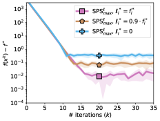
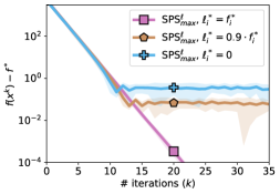
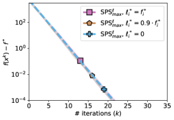
A numerical illustration of this result can be found in Fig. 1. In essence, both theory and experiments confirm that, if interpolation is not satisfied, then we have a linear rate until a convergence ball, where the size is optimal under exact knowledge of . Instead, under interpolation, if all the s are non-negative and , then SPSmax=SPS. Finally, in the less common case in practice where but we still have interpolation, then SPSmax converges to the exact solution while SPS does not. To conclude SPS does not (of course) work better than SPSmax, but it is a practical variant which we can use as a baseline in §5 for an adaptive stochastic Polyak stepsize with convergence to the true in the non-interpolated setting.
No Interpolation and Interpolation and Interpolation and
4 Bias in the SPS dynamics.
In this section, we study convergence of the standard SPSmax in the non-interpolated regime, under an additional (decreasing) multiplicative factor, in the most ideal setting: batch size 1, and we have knowledge of each . That is, we consider with , e.g. or . We note that, in the SGD case, simply picking e.g. would guarantee convergence of to , in expectation and with high probability [20, 23]. Therefore, it is natural to expect a similar behavior for SPS, if safisfies the usual Robbins-Monro conditions [27]: .
We show that this is not the case: quite interestingly, converges to a biased solution due to the correlation between and . we show this formally, in the case of non-interpolation (otherwise both SGD and SPS do not require a decreasing learning rate).
Counterexample.
Consider the following finite-sum setting: with . To make the problem interesting, we choose and : this introduces asymmetry in the average landscape with respect to the origin. During optimization, we sample and independently and seek convergence to the unique minimizer . The first thing we notice is that is not a stationary point for the dynamics under SPS. Indeed note that since for we have (assuming large enough): , if , and if .
Crucially, note that this update is curvature-independent. The expected update is . Hence, the iterates can only converge to — because this is the only fixed point for the update rule. The proof naturally extends to the multidimensional setting, an illustration can be found in Fig. 2.
No interpolation Interpolation
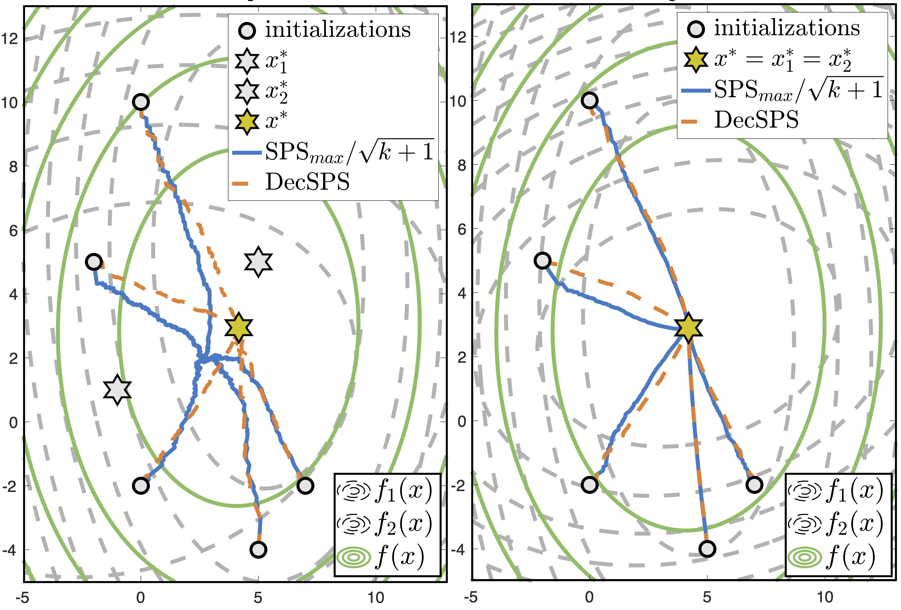
In the same picture, we show how our modified variant of the vanilla stepsize — we call this new algorithm DecSPS, see §5 — instead converges to the correct solution.
Remark 2.
SGD with (non-adaptive) stepsize instead keeps the curvature, and therefore is able to correctly estimate the average — precisely because is independent from . From this we can see that SGD can only converge to the correct stationary point — because again this is the only fixed point for the update rule.
In the appendix, we go one step further and provide an analysis of the bias of SPS in the one-dimensional quadratic case (Prop. 4). Yet, we expect the precise characterization of the bias phenomenon in the non-quadratic setting to be particularly challenging. We provide additional insights in §D.2. Instead, in the next section, we show how to effectively modify to yield convergence to without further assumptions.
5 DecSPS: Convergence to the exact solution
We propose the following modification of the vanilla SPS proposed in [22], designed to yield convergence to the exact minimizer while keeping the main adaptiveness properties222Similar choices are possible. We found that this leads to the biggest stepsize magnitude, allowing for faster convergence in practice.. We call it Decreasing SPS (DecSPS), since it combines a steady stepsize decrease with the adaptiveness of SPS.
for , where for every . We set and (stepsize bound, similar to [22]), to get .
Lemma 1.
Let each be smooth and let be any non-decreasing positive sequence of real numbers. Under DecSPS, we have , and
Remark 3.
As stated in the last lemma, under the assumption of non-decreasing, is trivially non-increasing since .
The proof can be found in the appendix, and is based on a simple induction argument.
5.1 Convergence under bounded iterates
The following result provides a proof of convergence of SGD for the sequence defined above.
Theorem 3.
Consider SGD with DecSPS and let be any non-decreasing sequence such that . Assume that each is convex and smooth. We have:
| (4) |
where , and .
If , then for all leads to a rate , well known from [22]. If , as for the standard SGD analysis under decreasing stepsizes, the choice leads to an optimal asymptotic trade-off between the deterministic and the stochastic terms, hence to the asymptotic rate since . Moreover, picking minimizes the speed of convergence for the deterministic factor. Under the assumption that (e.g. reasonable distance initialization-solution and ), this factor is dominant compared to the factor involving . For this setting, the rate simplifies as follows.
Corollary 2.
Under the setting of Thm. 3, for () we have
| (5) |
Remark 4 (Beyond bounded iterates).
The result above crucially relies on the bounded iterates assumption: . To the best of our knowledge, if no further regularity is assumed, modern convergence results for adaptive methods (e.g. variants of AdaGrad) in convex stochastic programming require333Perhaps the only exception is the result of [33], where the authors work on a different setting: i.e. they introduce the RUIG inequality. this assumption, or else require gradients to be globally bounded. To mention a few: [11, 26, 32, 8, 31]. A simple algorithmic fix to this problem is adding a cheap projection step onto a large bounded domain [21]. We can of course include this projection step in DecSPS, and the theorem above will hold with no further modification. Yet we found this to be not necessary: the strong guarantees of SPS in the strongly convex setting [22] let us go one step beyond: in §5.2 we show that, if each is strongly convex (e.g. regularizer is added), then one can bound the iterates globally with probability one, without knowledge of the gradient Lipschitz constant. To the best of our knowledge, no such result exist for AdaGrad — except [30], for the deterministic case.
Remark 5 (Dependency on the problem dimension).
In standard results for AdaGrad, a dependency on the problem dimension often appears (e.g. Thm. 1 in [31]). This dependency follows from a bound on the AdaGrad preconditioner that can be found e.g. in Thm. 4 in [21]. In the SPS case no such dependency appears — specifically because the stepsize is lower bounded by .
5.2 Removing the bounded iterates assumption
We prove that under DecSPS the iterates live in a set of diameter almost surely. This can be done by assuming strong convexity of each .
The result uses this alternative definition of neighborhood: .
Note that trivially under the assumption that all are lower bounded and .
Proposition 1.
Let each be -strongly convex and -smooth. The iterates of SGD with DecSPS with (and ) are such that almost surely , where , with and .
The proof relies on the variations of constants formula and an induction argument — it is provided in the appendix. We are now ready to state the main theorem for the unconstrained setting, which follows from Prop. 1 and Thm. 3.
Theorem 4.
Consider SGD with the DecSPS stepsize , for and defined as at the beginning of this section. Let each be -strongly convex and -smooth:
| (6) |
Remark 6 (Strong Convexity).
The careful reader might notice that, while we assumed strong convexity, our rate is slower than the optimal . This is due to the adaptive nature of DecSPS. It is indeed notoriously hard to achieve a convergence rate of for adaptive methods in the strongly convex regime. While further investigations will shed light on this interesting problem, we note that the result we provide is somewhat unique in the literature: we are not aware of any adaptive method that enjoys a similar convergence rate without either (a) assuming bounded iterates/gradients or (b) assuming knowledge of the gradient Lipschitz constant or the strong convexity constant.
Remark 7 (Comparison with Vanilla SGD).
On a convex problem, the non-asymptotic performance of SGD with a decreasing stepsize strongly depends on the choice of . The optimizer might diverge if is too big for the problem at hand. Indeed, most bounds for SGD, under no access to the gradient Lipschitz constant, display a dependency on the size of the domain and rely on projections after each step. If one applies the method in the unconstrained setting, such convergence rates technically do not hold, and tuning is sometimes necessary to retrieve stability and good performance. Instead, for DecSPS, simply by adding a small regularizer, the method is guaranteed to converge at the non-asymptotic rate we derived even in the unconstrained setting.
5.3 Extension to the non-smooth setting
For any , we denote in this section by the subgradient of evaluated at . We discuss the extension of DecSPS to the non-smooth setting.
A straightforward application of DecSPS leads to a stepsize which is no longer lower bounded (see Lemma 1) by the positive quantity . Indeed, the gradient Lipschitz constant in the non-smooth case is formally . Hence, prescribed by DecSPS can get arbitrarily small444Take for instance the deterministic setting one-dimensional setting . As , the stepsize prescribed by DecSPS converges to zero. This is not the case e.g. in the quadratic setting. for finite . One easy solution to the problem is to enforce a lower bound, and adopt a new proof technique. Specifically we propose the following:
where for every , is a small positive number and all the other quantities are defined as in DecSPS. In particular, as for DecSPS, we set and . Intuitively, is selected to live in the interval (see proof in §F, appendix), but has subgradient-dependent adaptive value. In addition, this stepsize is enforced to be monotonically decreasing.
Theorem 5.
For any non-decreasing positive sequence , consider SGD with DecSPS-NS. Assume that each is convex and lower bounded. We have
| (7) |
where and .
One can then easily derive an convergence rate. This is presented in §F (appendix).
6 Numerical Evaluation
We evaluate the performance of DecSPS with on binary classification tasks, with regularized logistic loss , where is the feature vector for the -th datapoint and is the corresponding binary target.
We study performance on three datasets: (1) a Synthetic
Dataset, (2) The A1A dataset [6] and (3) the
Breast Cancer dataset [10]. We choose
different regularization levels and batch sizes bigger than 1.
Details are reported in §G, and the code is available at https://github.com/aorvieto/DecSPS.
At the batch sizes and regularizer levels we choose, the problems do not satisfy interpolation. Indeed, running full batch gradient descent yields . While running SPSmax on these problems (1) does not guarantee convergence to and (2) requires full knowledge of the set of optimal function values , in DecSPS we can simply pick the lower bound for every . Supported by Theorems 3 & 4 & 5, we expect SGD with DecSPS to converge to the minimum .
Stability of DecSPS.
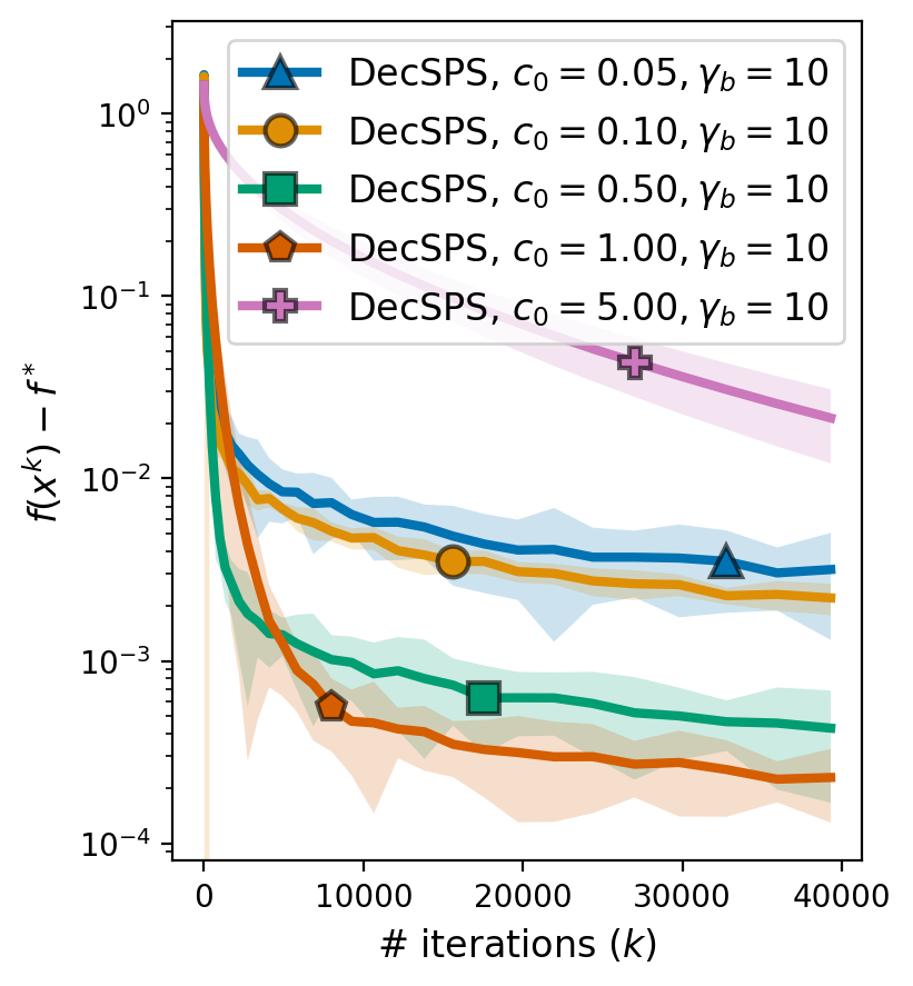
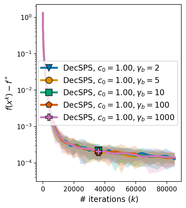
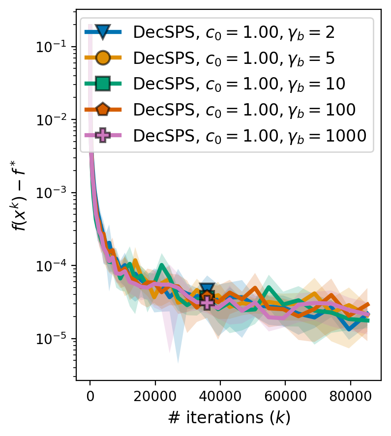
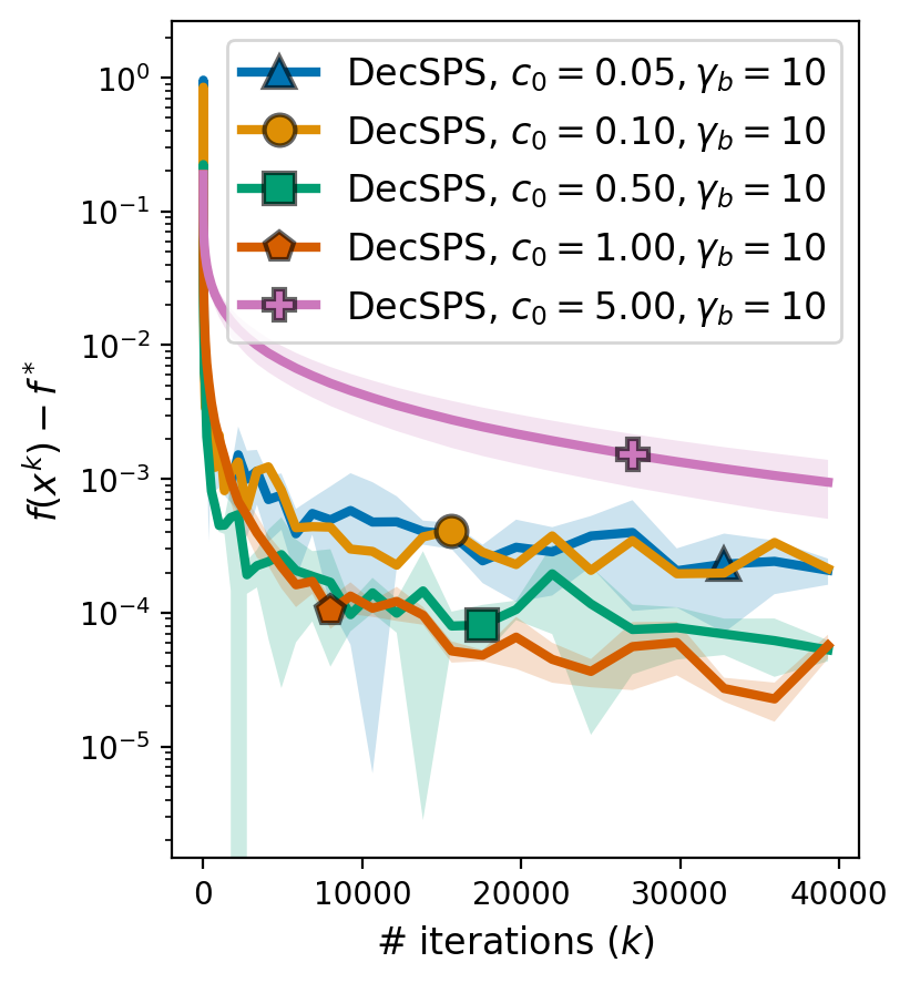
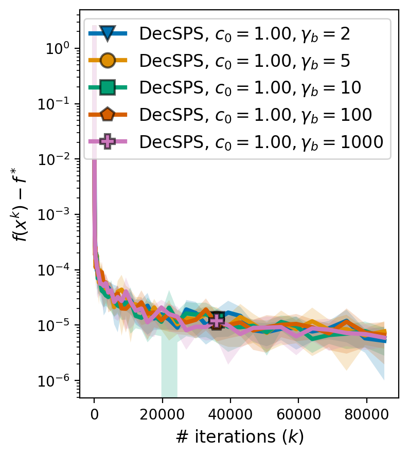
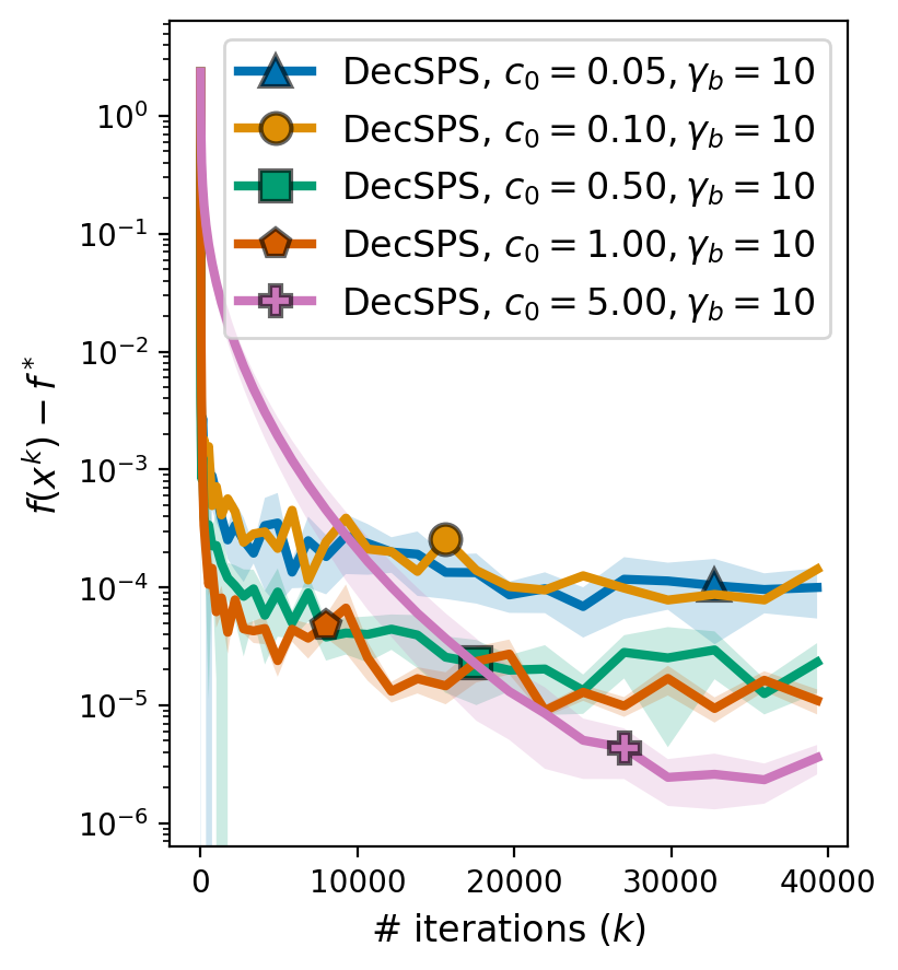
DecSPS has two hyperparameters: the upper bound on the first stepsize and the scaling constant . While Thm. 5 guarantees convergence for any positive value of these hyperparameters, the result of Thm. 3 suggests that using yields the best performance under the assumption that (e.g. reasonable distance of initialization from the solution, and ). In Fig. 3, we show on the synthetic dataset that (1) is indeed the best choice in this setting and (2) the performance of SGD with DecSPS is almost independent of . Similar findings are reported and commented in Figure 7 (Appendix) for the other datasets. Hence, for all further experiments, we choose the hyperparameters .
Comparison with vanilla SGD with decreasing stepsize.
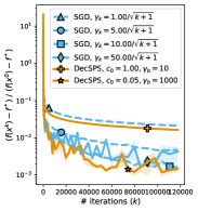
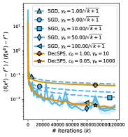
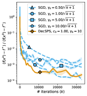
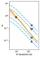
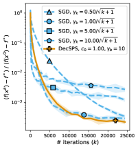
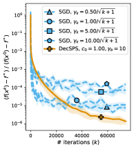
We compare the performance of DecSPS against the classical decreasing SGD stepsize , which guarantees convergence to the exact solution at the same asymptotic rate as DecSPS. We show that, while the asymptotics are the same, DecSPS with hyperparameters performs competitively to a fine-tuned — where crucially the optimal value of depends on the problem. This behavior is shown on all the considered datasets, and is reported in Figures 4 (Breast and Synthetic reported in the appendix for space constraints). If lower regularization () is considered, then DecSPS can still match the performance of tuned SGD — but further tuning is needed (see Figure 14. Specifically, since the non-regularized problems do not have strong curvature, we found that DecSPS works best with a much higher parameter and .
DecSPS yields a truly adaptive stepsize.
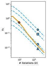
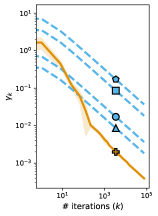
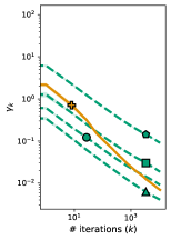
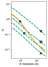
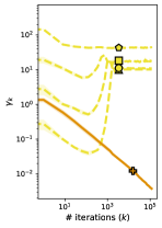
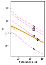
We inspect the value of returned by DecSPS, shown in Figures 4 & 8 (in the appendix). Compared to the vanilla SGD stepsize , a crucial difference appears: decreases faster than . This showcases that, while the factor can be found in the formula of DecSPS555We pick , as suggested by Cor. 2 & 3 , the algorithm structure provides additional adaptation to curvature. Indeed, in (regularized) logistic regression, the local gradient Lipschitz constant increases as we approach the solution. Since the optimal stepsize for steadily-decreasing SGD is , where is the global Lipschitz constant [13], it is pretty clear that should be decreased over training for optimal converge (as effectively increases). This is precisely what DecSPS is doing.
Comparison with AdaGrad stepsizes.
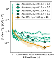
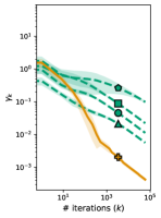
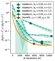
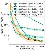
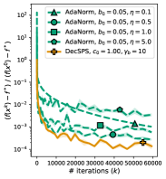
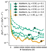
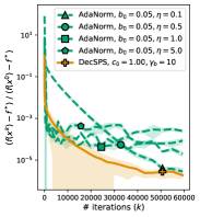
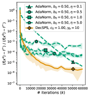
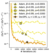
Last, we compare DecSPS with another adaptive coordinate-independent stepsize with strong theoretical guarantees: the norm version of AdaGrad (a.k.a. AdaGrad-Norm, AdaNorm), which guarantees the exact solution at the same asymptotic rate as DecSPS [32]. AdaGrad-norm at each iteration updates the scalar and then selects the next step as . Hence, it has tuning parameters and . In Fig. 4 we show that, on the Breast Cancer dataset, after fixing as recommended in [32] (see their Figure 3), tuning cannot quite match the performance of DecSPS. This behavior is also observed on the other two datasets we consider (see Fig. 9 in the Appendix). Last, in Fig. 10& 11 in the Appendix, we show that further tuning of likely does not yield a substantial improvement.
Regularized A1A – SGD Vs DecSPS Regularized Breast Cancer – AdaGrad-Norm VS DecSPS
Comparison with Adam and AMSgrad without momentum.
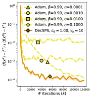
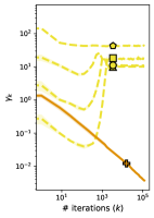
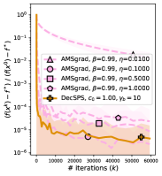
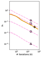
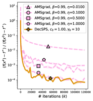
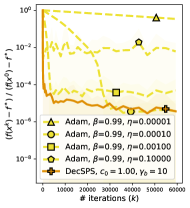
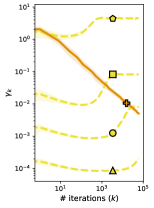
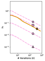
In Figures 5&12&13 we compare DecSPS with Adam [19] and AMSgrad [26] on the A1A and Breast Cancer datasets. Results show that DecSPS with the usual hyperparameters is comparable to the fine-tuned version of both these algorithms — which however do not enjoy convergence guarantees in the unbounded domain setting.
Regularized A1A – DecSPS Vs Adam Regularized Breast Cancer – DecSPS Vs AMSgrad
7 Conclusions and Future Work
We provided a practical variant of SPS [22], which converges to the true problem solution without the interpolation assumption in convex stochastic problems — matching the rate of AdaGrad. If in addition, strong convexity is assumed, then we show how, in contrast to current results for AdaGrad, the bounded iterates assumption can be dropped. The main open direction is a proof of a faster rate under strong convexity. Other possible extensions of our work include using the proposed new variants of SPS with accelerated methods, studying further the effect of mini-batching and non-uniform sampling of DecSPS, and extensions to the distributed and decentralized settings.
Acknowledgements
This work was partially supported by the Canada CIFAR AI Chair Program. Simon Lacoste-Julien is a CIFAR Associate Fellow in the Learning in Machines & Brains program.
References
- Asi and Duchi [2019a] H. Asi and J. C. Duchi. The importance of better models in stochastic optimization. Proceedings of the National Academy of Sciences, 116(46):22924–22930, 2019a.
- Asi and Duchi [2019b] H. Asi and J. C. Duchi. Stochastic (approximate) proximal point methods: Convergence, optimality, and adaptivity. SIAM Journal on Optimization, 29(3):2257–2290, 2019b.
- Berrada et al. [2020] L. Berrada, A. Zisserman, and M. P. Kumar. Training neural networks for and by interpolation. In International Conference on Machine Learning, 2020.
- Bottou et al. [2018] L. Bottou, F. E. Curtis, and J. Nocedal. Optimization methods for large-scale machine learning. Siam Review, 60(2):223–311, 2018.
- Boyd et al. [2003] S. Boyd, L. Xiao, and A. Mutapcic. Subgradient methods. Lecture Notes of EE392o, Stanford University, Autumn Quarter, 2004:2004–2005, 2003.
- Chang [2011] C.-C. Chang. LIBSVM: a library for support vector machines. ACM Transactions on Intelligent Systems and Technology, 2011.
- Davis et al. [2018] D. Davis, D. Drusvyatskiy, K. J. MacPhee, and C. Paquette. Subgradient methods for sharp weakly convex functions. Journal of Optimization Theory and Applications, 179(3):962–982, 2018.
- Défossez et al. [2020] A. Défossez, L. Bottou, F. Bach, and N. Usunier. A simple convergence proof of Adam and Adagrad. arXiv preprint arXiv:2003.02395, 2020.
- D’Orazio et al. [2021] R. D’Orazio, N. Loizou, I. Laradji, and I. Mitliagkas. Stochastic mirror descent: Convergence analysis and adaptive variants via the mirror stochastic Polyak stepsize. arXiv preprint arXiv:2110.15412, 2021.
- Dua and Graff [2017] D. Dua and C. Graff. UCI machine learning repository, 2017. URL http://archive.ics.uci.edu/ml.
- Duchi et al. [2011] J. Duchi, E. Hazan, and Y. Singer. Adaptive subgradient methods for online learning and stochastic optimization. Journal of Machine Learning Research, 12(7), 2011.
- Ene and Nguyen [2020] A. Ene and H. L. Nguyen. Adaptive and universal algorithms for variational inequalities with optimal convergence. arXiv preprint arXiv:2010.07799, 2020.
- Ghadimi and Lan [2013] S. Ghadimi and G. Lan. Stochastic first-and zeroth-order methods for nonconvex stochastic programming. SIAM Journal on Optimization, 23(4), 2013.
- Goodfellow et al. [2016] I. Goodfellow, Y. Bengio, and A. Courville. Deep Learning. MIT press, 2016.
- Gower et al. [2021a] R. Gower, O. Sebbouh, and N. Loizou. SGD for structured nonconvex functions: Learning rates, minibatching and interpolation. In International Conference on Artificial Intelligence and Statistics, 2021a.
- Gower et al. [2019] R. M. Gower, N. Loizou, X. Qian, A. Sailanbayev, E. Shulgin, and P. Richtárik. SGD: General analysis and improved rates. In International Conference on Machine Learning, 2019.
- Gower et al. [2021b] R. M. Gower, A. Defazio, and M. Rabbat. Stochastic Polyak stepsize with a moving target. arXiv preprint arXiv:2106.11851, 2021b.
- Hazan and Kakade [2019] E. Hazan and S. Kakade. Revisiting the Polyak step size. arXiv preprint arXiv:1905.00313, 2019.
- Kingma and Ba [2014] D. P. Kingma and J. Ba. Adam: A method for stochastic optimization. arXiv:1412.6980, 2014.
- Kushner and Yin [2003] H. Kushner and G. G. Yin. Stochastic Approximation and Recursive Algorithms and Applications, volume 35. Springer Science & Business Media, 2003.
- Levy et al. [2018] K. Y. Levy, A. Yurtsever, and V. Cevher. Online adaptive methods, universality and acceleration. Advances in Neural Information Processing Systems, 31, 2018.
- Loizou et al. [2021] N. Loizou, S. Vaswani, I. H. Laradji, and S. Lacoste-Julien. Stochastic Polyak step-size for SGD: An adaptive learning rate for fast convergence. In International Conference on Artificial Intelligence and Statistics, 2021.
- Nemirovski et al. [2009] A. Nemirovski, A. Juditsky, G. Lan, and A. Shapiro. Robust stochastic approximation approach to stochastic programming. SIAM Journal on Optimization, 19(4):1574–1609, 2009.
- Oberman and Prazeres [2019] A. M. Oberman and M. Prazeres. Stochastic gradient descent with Polyak’s learning rate. arXiv preprint arXiv:1903.08688, 2019.
- Polyak [1987] B. Polyak. Introduction to Optimization. Inc., Publications Division, New York, 1987.
- Reddi et al. [2018] S. J. Reddi, S. Kale, and S. Kumar. On the convergence of Adam and beyond. In International Conference on Learning Representations, 2018.
- Robbins and Monro [1951] H. Robbins and S. Monro. A stochastic approximation method. The Annals of Mathematical Statistics, 1951.
- Rolinek and Martius [2018] M. Rolinek and G. Martius. L4: Practical loss-based stepsize adaptation for deep learning. Advances in neural information processing systems, 31, 2018.
- Tieleman and Hinton [2012] T. Tieleman and G. Hinton. Lecture 6.5 - RMSprop, Coursera: Neural networks for machine learning. University of Toronto, Technical Report, 2012.
- Traoré and Pauwels [2021] C. Traoré and E. Pauwels. Sequential convergence of AdaGrad algorithm for smooth convex optimization. Operations Research Letters, 49(4):452–458, 2021.
- Vaswani et al. [2020] S. Vaswani, I. Laradji, F. Kunstner, S. Y. Meng, M. Schmidt, and S. Lacoste-Julien. Adaptive gradient methods converge faster with over-parameterization (but you should do a line-search). arXiv preprint arXiv:2006.06835, 2020.
- Ward et al. [2019] R. Ward, X. Wu, and L. Bottou. Adagrad stepsizes: Sharp convergence over nonconvex landscapes. In International Conference on Machine Learning, 2019.
- Xie et al. [2020] Y. Xie, X. Wu, and R. Ward. Linear convergence of adaptive stochastic gradient descent. In International Conference on Artificial Intelligence and Statistics, 2020.
- Zhang et al. [2021] C. Zhang, S. Bengio, M. Hardt, B. Recht, and O. Vinyals. Understanding deep learning (still) requires rethinking generalization. Communications of the ACM, 64(3):107–115, 2021.
- Zhang et al. [2020] J. Zhang, S. P. Karimireddy, A. Veit, S. Kim, S. Reddi, S. Kumar, and S. Sra. Why are adaptive methods good for attention models? Advances in Neural Information Processing Systems, 33, 2020.
Supplementary Material
Dynamics of SGD with Stochastic Polyak Stepsizes:
Truly Adaptive Variants and Convergence to Exact Solution
The appendix is organized as follows:
-
1.
In §A we provide a more detail comparison with closely related works.
-
2.
In §B we present some technical preliminaries.
-
3.
In §C, we present convergence guarantees for SPS after replacing with (lower bound).
-
4.
In §D, we discuss the lack of convergence of SPS in the non-interpolated setting.
-
5.
In §E, we discuss convergence of DecSPS, our convergent variant of SPS.
-
6.
In §F, we discuss convergence of DecSPS-NS, our convergent variant of SPS in the non-smooth setting.
-
7.
In §G we provide some additional experimental results and describe the datasets in detail.
Appendix A Comparison with closely related work
In this section we present a more detailed comparison to closely related works on stochastic variants of the Polyak stepsize. We start with the work of Asi and Duchi [2], and then continue with a brief presentation of other papers (already presented in Loizou et al. [22]).
A.1 Comparison with Asi and Duchi [2]
Asi and Duchi [2] proposed the following adaptive method for solving Problem (1) under the interpolation assumption for all subsets of with :
| (8) |
where for some , is a polynomially decreasing/increasing sequence. We provide here a full comparison of this stepsize with SPS and DecSPS.
Comparison with the adaptive stepsizes in Loizou et al. [22] and our DecSPS.
In Loizou et al. [22], the proposed SPSmax stepsize is
| (9) |
This stepsize is similar to the one in Asi and Duchi [2]: in both, a Polyak-like stochastic stepsize is bounded from above in order to guarantee convergence. However there are crucial differences.
- •
-
•
As we will see in the next paragraph, one can formulate few conditions under which it is possible to derive linear convergence rates for Eq. (8) in the interpolated setting. As can be easily seen from Theorem 1, SPSmax has similar convergence guarantees but works under a more standard/restrictive set of assumptions. In particular, in the interpolated setting, while Asi and Duchi [2] require some specific assumptions on the noise statistics (see next paragraph), the rates in Loizou et al. [22] can be applied without the need for, e.g., probabilistic bound on the gradient magnitude.
In this paper, starting from the SPSmax algorithm we propose the following stepsize for convergence to the exact solution in the non-interpolated setting:
| (DecSPS) |
where is an increasing sequence (e.g. , see Theorem 4), and is any lower bound on . At initialization, we set and .
We now compare DecSPS with Eq. (8) and our results with the rates in [2].
-
•
Convergence rates: The form of Eq. (8) and the convergence guarantees of [2] are restricted to the interpolated setting. Instead, in this paper we focus on the non-interpolated setting: using DecSPS we provided the first stochastic adaptive optimization method that converges in the non-interpolated setting to the exact solution without restrictive assumptions like bounded iterates/gradients.
-
•
Inspection of the stepsize: DecSPS provides a version of SPS where is steadily decreasing and is upper bounded by the decreasing quantity , where yields the optimal asymptotic rate (Theorem 4) . Hence, DecSPS can be compared to Eq. (8) for . However, note that there are two fundamental differences: First, in DecSPS we have that (see Lemma 1), a feature which Eq. (8) does not have. Secondly, compared to our DecSPS, the stepsize in Eq. (8) with decreasing polynomially is asymptotically non-adaptive. Indeed, assuming that each has -Lipschitz gradients and that each is non-negative, we have (see [22]) that
(10) therefore, after iterations666Simply plugging in and solving for . the algorithm coincides with SGD with stepsize .
For completeness, we provide in the next paragraph an overview of the results in Asi and Duchi [2].
Precise theoretical guarantees in Asi and Duchi [2].
The stepsize in Equation (8) yields linear convergence guarantees under a specific set of assumptions. We summarize the two main results of Asi and Duchi [2] below in the case of differentiable losses777The results of Asi and Duchi [2] also work in the subdifferentiable setting.:
Proposition 2 (Proposition 2 in Asi and Duchi [2]).
Let each be a convex and differentiable function which satisfies a specific set of technical assumptions (see conditions C.i and C.iii in [2]). For a fixed batch-size assume for all subsets of with (i.e. interpolation). Assume in addition that there exist constants such that for all , and (set of solutions) we have (sharp growth with shared minimizers assumption)
| (11) |
Then, for with the stepsize of Equation (8) yields a linear convergence rate dependent on and the choice of .
Sufficient conditions for Equation (11) to hold is that there exist such that, for all , and .
Proposition 3 (Proposition 3 in Asi and Duchi [2]).
Let each be a convex and differentiable function which satisfies a specific set of technical assumptions (see conditions C.i and C.iii in [2]). Under the same interpolation assumptions as Lemma 2, assume that there exist constants such that for all , and we have (quadrtic growth with shared minimizers assumption)
| (12) |
Then, for with the stepsize of Equation (8) yields a linear convergence rate dependent on and the choice of .
The authors show that Equation (12) holds under the assumption that the averaged loss has quadratic growth and has Lipschitz continuous gradients, if in addition there exist constants , such that .
A.2 Comparisons with other versions of the Polyak stepsize for stochastic problems
To the best of our knowledge, no prior work has provided a computationally feasible modification of the Polyak stepsize for convergence to the exact solution in stochastic non-interpolated problems. In the next lines, we outline the details for a few related works on Polyak stepsize for stochastic problems.
-
•
SPSmax: As discussed in the main paper, our starting point is the SPSmax algorithm in [22], which provides linear (for strongly convex) or sublinear (for convex) convergence to a ball around the minimizer, with size dependent of the problems’ degree of interpolation. Instead, in this work, we provide convergence guarantees to the exact solution in the non-interpolated setting for a modified version of this algorithm. In addition, when compared to SPSmax, our method does not require knowledge of the single s, but just of lower bounds on these quantities (see §3).
-
•
L4: A stepsize very similar to SPSmax (the L4 algorithm) was proposed back in 2018 by [28]. While this stepsize results in promising performance in deep learning, (1) it has no theoretical convergence guarantees, and (2) each update requires an online estimation of the , which in turn requires tuning up to three hyper-parameters.
-
•
SPLR: Oberman and Prazeres [24] instead study convergence of SGD with the following stepsize: , which requires knowledge of for all iterates and the evaluation of — the full-batch loss — at each step. This makes the concrete application of SPLR problematic for sizeable stochastic problems.
-
•
ALI-G: Last, the ALI-G stepsize proposed by Berrada et al. [3] is , where is a tuning parameter. Unlike the SPSmax setting, their theoretical analysis relies on an -interpolation condition. Moreover, the values of the parameter and that guarantee convergence heavily depend on the smoothness parameter of the objective , limiting the method’s practical applicability. In addition, in the interpolated setting, while ALI-G converges to a neighborhood of the solution, the SPSmax method [22] is able to provide linear convergence to the solution.
Appendix B Technical Preliminaries
Let us present some basic definitions used throughout the paper.
Definition 1 (Strong Convexity / Convexity).
The function , is -strongly convex, if there exists a constant such that :
| (13) |
for all . If inequality (13) holds with the function is convex.
Definition 2 (-smooth).
The function , -smooth, if there exists a constant such that :
| (14) |
or equivalently:
| (15) |
Lemma 2.
If a function is -strongly convex and -smooth the following bounds holds:
| (16) |
The following lemma is the fundamental starting point in [22].
Lemma 3.
Let where the functions are -strongly convex and -smooth, then
| (17) |
where , and .
Proof.
Directly using Lemma 2. ∎
Appendix C Convergence guarantees after replacing in SPS with
The proofs in this subsection is an easy adaptation of the proofs appeared in [22]. To avoid redundancy in the literature, we provide skecth of the proofs showing the fundamental differences and invite the interested reader to read the details in [22].
See 2
Proof.
We highlight in blue text the differences between this proof and the one in [22].
Recall the stepsize definition
| (SPS) |
where is any lower bound on . We also will make use of the bound
| (18) |
Convex setting.
As in [22] we use a standard expansion as well as the stepsize definition.
| (19) | |||
| (20) | |||
| (21) | |||
| (22) | |||
| (23) |
Next, adding and subtracting gives
| (25) | |||
| (26) | |||
| (27) | |||
| (28) |
Since it holds that . We obtain:
| (29) | |||
| (30) | |||
| (31) | |||
| (32) | |||
| (33) | |||
| (34) | |||
| (35) |
where in the last inequality we use that . Note that this factor pops up in the proof, not in the stepsize! By rearranging:
| (36) |
The rest of the proof is identical to [22] (Theorem 3.4). Just, at the instead of we have . That is, after taking the expectation on both sides (conditioning on ), we can use the tower property and sum over (from to ) on both sides of the inequality. After dividing by , thanks to Jensen’s inequality, we get (for ):
where , and is the maximum smoothness constant.
Strongly Convex setting.
We proceed in the usual way:
| (37) | ||||
| (38) |
Using the fact that , we get
| (40) | |||
| (41) | |||
| (42) |
From convexity of functions it holds that , . Thus,
| (43) | ||||
| (44) |
The rest of the proof is identical to [22] (Theorem 3.1). Just, at the instead of we have . That is, after taking the expectation on both sides (conditioning on ), we can use the tower property and solve the resulting geometric series in closed form: for we get
where and is the maximum smoothness constant. ∎
Appendix D Lack of convergence of SGD with SPSmax in the non-interpolated setting
D.1 Convergence of SPS with decreasing stepsizes to in the quadratic case
We recall the variation of constants formula
Lemma 4 (Variation of constants).
Let evolve with time-varying linear dynamics , where and for all . Then, with the convention that ,
| (45) |
Proof.
For we get . The induction step yields
| (46) | ||||
| (47) | ||||
| (48) | ||||
| (49) |
This completes the proof of the variations of constants formula. ∎
Proposition 4 ( Quadratic 1d).
Consider . We consider SGD with , with . Then , with
Proof.
To show that , first notice that the curvature gets canceled out in the update, due to correlation between and .
| (50) |
Now let’s add and subtract twice as follows:
| (51) |
From this equality it is already clear that in expectation the update is in the direction of . To provide a formal proof of convergence the first step is to use the variations of constants formula ( Lemma 4). Therefore,
| (52) |
If then and therefore
| (53) |
Hence,
| (54) |
Moreover, since we have that in distribution, by the law of large numbers.
Finally, to get a rate on the distance-shrinking, we take the expectation w.r.t. conditioned on : the cross-term disappears and we get
| (55) | ||||
| (56) |
Plugging in , we get
| (57) |
Therefore, using the tower property and the variation of constants formula,
| (58) | ||||
| (59) |
This concludes the proof. ∎
D.2 Asymptotic vanishing of the SPS bias in 1d quadratics
As the number of datapoints grows, the bias in the SPS solution (Prop. 4) is alleviated by an averaging effect. Indeed, if we let each pair to be sampled i.i.d, for every we have
| (60) |
As , it is possible to see that, under some additional assumptions (e.g. Beta-distributed), the variance of collapses to zero, hence one has in probability, as , with rate .
First, recall the law of total variance: . In our case, setting and , the first term is zero since is independent of . Hence
| (61) | |||
| (62) |
Evaluating might be complex, yet if e.g. one assumes e.g. (positive support, to ensure convexity), then it is possible to show888This derivation was posted on the Mathematics StackExchange at https://math.stackexchange.com/questions/138290/finding-e-left-frac-sum-i-1n-x-i2-sum-i-1n-x-i2-right-of-a-sam?rq=1 and we report it here for completeness. that . First, recall that, for ,
| (63) |
We rewrite the expectation as follows:
| (64) | ||||
| (65) | ||||
| (66) | ||||
| (67) |
where denotes the moment generating function of the distribution. Next, we solve the integral using the closed-form expression for (else does not exist). Note that we integrate only for so the MGF is always defined:
| (68) | ||||
| (69) | ||||
| (70) | ||||
| (71) | ||||
| (72) |
where in the third-last inequality we changed variables and in the second last we changed variables .
All in all, we have that . This implies that converges to in quadratic mean — hence also in probability.
Appendix E Convergence of SGD with DecSPS in the smooth setting
Here we study Decreasing SPS (DecSPS), which combines stepsize decrease with the adaptiveness of SPS.
| (DecSPS) |
for , where we set and (stepsize bound, similar to [22]), to get
| (73) |
E.1 Proof of Lemma 1
See 1
Proof.
First, note that is trivially non-increasing since . Next, we prove the bounds on .
For , we can directly use Lemma 2:
| (74) |
Next, we proceed by induction: we assume the proposition holds true for :
| (75) |
Then, we have : , where
| (76) |
by the induction hypothesis. This bound directly implies that the proposition holds true for , since again by Lemma 2 we have . This concludes the induction step. ∎
E.2 Proof of Thm. 3
Remark 8 (Why was this challenging?).
The fundamental problem towards a proof for DecSPS is that the error to control due to gradient stochasticity does not come from the term in the expansion of , as instead is usual for SGD with decreasing stepsizes. Instead, the error comes from the inner product term . Hence, the error is proportional to , and not . As a result, the usual Robbins-Monro conditions [27] do not yield convergence. A similar problem is discussed for AdaGrad in [32].
In the first version of this paper, the proof contained a small error999This was in Eq. (87), where we incorrectly bounded with the constant . This, of course, cannot be done since the term is not positive. However, it’s expectation is positive. Since is a constant, we avoid bounding it in the early stages and instead bound it after taking the expectation at the end of the proof. The result is unchanged.. This is now fixed, the result is unchanged.
See 3
Proof.
Note that from the definition , we have that:
| (77) |
Multiplying by and rearranging terms we get the fundamental inequality
| (78) |
Using the definition of DecSPS and convexity we get
| (79) | |||
| (80) | |||
| (81) |
Next, using convexity,
| (82) | |||
| (83) | |||
| (84) | |||
| (85) |
Let us divide everything by .
| (86) |
Rearranging,
| (87) |
Next, summing from to :
| (88) |
And therefore
| (89) | |||
| (90) | |||
| (91) | |||
| (92) | |||
| (93) | |||
| (94) | |||
| (95) |
Remark 9 (Where did we use the modified SPS definition?).
Remark 10 (Second term does not depend on ).
Note that, in the convergence rate, the second term does not depend on while the first does. This is different from the original SPS result [22], and due to the different proof technique: specifically, we divide by early in the proof — and not at the end. To point to the exact source of this difference, we invite the reader to inspect Equation 24 in the appendix101010http://proceedings.mlr.press/v130/loizou21a/loizou21a-supp.pdf of [22]: the last term there is proportional to , where is a lower bound on the SPS and is an upper bound. In our proof approach, these terms — which bound the same quantity — effectively cancel out (because we divide by earlier in the proof), at the price of having in the first term.
E.3 Proof of Prop. 1
We need the following lemma. An illustration of the result can be found in Fig. 6.
Lemma 5.
Let with and . If , , , then for all .
Proof.
Simple to prove by induction. The base case is trivial, since . Let us now assume the proposition holds true for (that is, ) , we want to show it holds true for . We have
| (101) |
If , then we get, by induction
| (102) |
Else, if , then by induction
| (103) |
where the last inequality holds because and is positive. This completes the proof. ∎
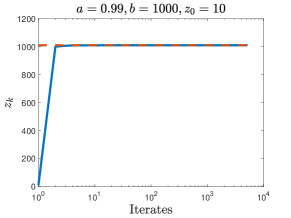
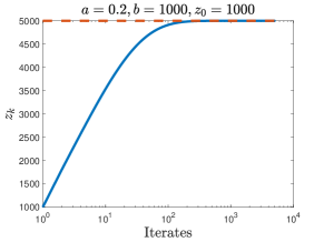
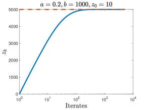
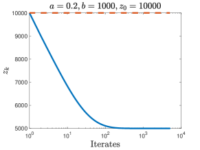
See 1
Proof.
Using the SPS definition we directly get
| (104) | ||||
| (105) | ||||
| (106) |
where (as always) we used the fact that since from the definition , then and we have
| (107) |
Now recall that, if each is -strongly convex then for any we have
| (108) |
For and , this implies
| (109) |
Adding and subtracting to the RHS of the inequality above, we get
| (110) |
Since , we can substitute this inequality in Equation (106) and get
| (111) | ||||
| (112) |
Rearranging a few terms we get
| (113) | |||
| (114) | |||
| (115) |
Since we assumed for all , we can drop the term , since also . Hence, we get the following bound:
| (116) | ||||
| (117) | ||||
| (118) |
where we used the inequality (Lemma 1).
Appendix F Convergence of stochastic subgradient method with DecSPS-NS in the non-smooth setting
In this subsection we consider the DecSPS-NS stepsize in the non-smooth setting:
| (121) |
where is the stochastic subgradient using batch size at iteration , and we set and to get
| (122) |
F.1 Proof stepsize bounds
Lemma 6 (Non-smooth bounds).
Let be any non-decreasing positive sequence. Then, under DecSPS-NS, we have that for every , , .
Proof.
First, note that is trivially non-increasing since . Next, we prove the bounds on .
Without loss of generality, we can work with the simplified stepsize
| (123) |
where is any number. We proceed by induction: at (base case) we get
| (124) |
if then . Otherwise and therefore . If in addition, if then , else . In all these cases, we get ; hence, the base case holds true.
We now proceed with the induction step by assuming . Using the definition of DecSPS-NS we will then show that the same inequalities hold for . We start by noting that, since , it holds that,
| (125) |
Similarly to the base case, we can write:
| (126) |
With a procedure identical to the setting we get that . This concludes the proof. ∎
F.2 Proof of Thm. 5
See 5
Proof.
Let us consider the DecSPS stepsize in the non-smooth setting. Using convexity and the gradient bound we get
| (127) | ||||
| (128) | ||||
| (129) |
where the last line follows from definition of subgradient and Lemma 6.
By dividing by ,
| (130) |
Using the same exact steps as Thm 3, and using the fact that is decreasing, we arrive at the equation
| (131) |
Now we use the fact that, since by Lemma 6, we have
| (132) |
We conclude by taking the expectation and using Jensen’s inequality. ∎
Corollary 3.
In the setting of Thm. 5, if we have
| (133) |
Remark 11.
The bound in Cor. 3 does not depend on , while the one in Cor. 2 does. This is because the proof is different, and does not rely on bounding squared gradients with function suboptimalities (one cannot, if smoothness does not hold). Similarly, usual bounds for non-smooth optimization do not depend on subgradient variance but instead on [23, 11, 12].
Appendix G Further experimental results
-
•
Synthetic Dataset : Following [16] we generate datapoints from a standardized Gaussian distribution in , with . We sample the corresponding labels at random. We consider a batch size and either or .
-
•
A1A dataset (standard normalization) from [6], consisting in datapoints in 123 dimensions. We consider again but a substantial regularization with .
-
•
Breast Cancer dataset (standard normalization) [10], consisting in datapoints in 39 dimensions. We consider a small batch size with strong regularization .
All experiments reported below are repeated 5 times. Shown is mean and 2 standard deviations.
Tuning of DecSPS.
DecSPS has two hyperparameters: the upper bound on the first stepsize and the scaling constant . As stated in the main paper, while Thm. 5 guarantees convergence for any positive value of these hyperparameters, the result of Thm. 3 suggests that using yields the best performance under the assumption that (e.g. reasonable distance of initialization from the solution, and the maximum gradient Lipschitz constant ). For the definition of these quantities plese refer to the main paper. In Fig. 3 in the main paper we showed that (1) is optimal in this setting (under and (2) the performance of SGD with DecSPS is almost independent of at . Similar findings hold for the A1A and Breast Cancer datasets, as shown in Figure 7. For A1A, we can see that the dynamics is almost independent of at and that, at , indeed yields the best performance. The findings are similar for the Breast Cancer dataset; however, there we see that at , yields the best final suboptimality — yet is clearly the best tradeoff between convergence speed and final accuracy.
A1A - Sensitivity A1A - Sensitivity Breast - Sensitivity Breast - Sensitivity
Comparison with SGD.
In addition to Figure 4 (A1A dataset), in Figure 8 we provide comparison of DecSPS with SGD with stepsize for the Synthetic and Breast Cancer datasets. From the results, it is clear that DecSPS with standard parameters (see discussion in main paper and paragraph above) is comparable if not faster than vanilla SGD with decreasing stepsize.
Synthetic Logistic Regression – SGD Vs DecSPS Regularized Breast Cancer – SGD Vs DecSPS
Comparison with Adagrad-Norm.
In addition to Figure 4 (Breast Cancer dataset), in Figures 10&11&9 we provide comparison of DecSPS with AdaGrad-Norm [32] for the Synthetic and A1A datasets. AdaGrad-norm at each iteration updates the scalar and then selects the next step as . Hence, it has tuning parameters and ; is recommended in [32] (see their Figure 3). Using this value for we show in Figure 9 that the performance of DecSPS is competitive against a well-tuned value of the AdaGrad-norm stepsize . In Figure 10&11 we show the effect of tuning on the synthetic dataset: no major improvement is observed.
Regularized A1A – DecSPS Vs AdaGrad-Norm Synthetic Dataset – DecSPS Vs AdaGrad-Norm
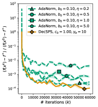
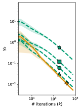
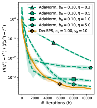
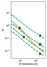
Synthetic Logistic Regression, Synthetic Logistic Regression,
Regularized A1A, Regularized Breast Cancer ,
Comparison with Adam and AMSgrad.
We provide a comparison with Adam [19] and AMSgrad [26]. For both methods, we set the momentum parameter to zero (a.k.a RMSprop) for a fair comparison with DecSPS. For , the parameter that controls the moving average of the second moments, we select the value since we found that the standard leads to problematic (exploding) stepsizes. Findings are pretty similar for both the A1A (Figure 12) and Breast Cancer (Figure 13) datasets: when compared to DecSPS with the usual parameters, fine-tuned Adam with fixed stepsize can reach the same performance after a few tens of thousand iterations — however, it is much slower at the beginning of training. While deriving convergence guarantees for Adam is problematic [26], AMSgrad [26] with stepsize enjoys a convergence guarantee similar to Adagrad and Adagrad-Norm. This is reflected in the empirical convergence: fine-tuned AMSgrad is able to match the convergence of DecSPS with the usual parameters motivated at the beginning of this section. Yet, we recall that the convergence guarantees of AMSgrad require the iterates to live in a bounded domain, an assumption which is not needed in our DecSPS (see § 5.2).
Regularized A1A – DecSPS Vs Adam Regularized A1A – DecSPS Vs AMSgrad
Regularized Breast Cancer – DecSPS Vs Adam Regularized Breast Cancer – DecSPS Vs AMSgrad

Performance under light regularization.
If the problem at hand does not have strong curvature information, e.g. there is very light regularization, then additional tuning of the DecSPS parameters is required. Figure 14 shows that it is possible to retrieve the performance of SGD also with light regularization parameters () under additional tuning of and .
SGD vs DecSPS on A1A with lighter regularization
