Informed Steiner Trees: Sampling and Pruning for Multi-Goal Path Finding in High Dimensions

Abstract

We interleave sampling based motion planning methods with pruning ideas from minimum spanning tree algorithms to develop a new approach for solving a Multi-Goal Path Finding (MGPF) problem in high dimensional spaces. The approach alternates between sampling points from selected regions in the search space and de-emphasizing regions that may not lead to good solutions for MGPF. Our approach provides an asymptotic, 2-approximation guarantee for MGPF. We also present extensive numerical results to illustrate the advantages of our proposed approach over uniform sampling in terms of the quality of the solutions found and computation speed.

Introduction

Multi-Goal Path Finding (MGPF) problems aim to find a least-cost path for a robot to travel from an origin ($s$) to a destination ($d$) such that the path visits each node in a given set of goals ($\bar{T}$) at least once. In the process of finding a least-cost path, MGPF algorithms also find an optimal sequence in which the goals must be visited. When the search space is discrete ($i.e.$, a finite graph), the cost of traveling between any two nodes is computed using an all-pairs shortest paths algorithm. In this case, the MGPF encodes a variant of the Steiner Traveling Salesman Problem (TSP) and is NP-Hard (Kou, Markowsky, and Berman 1981). In the general case, the search space is continuous and the least cost to travel between any two nodes is not known a-priori. This least-cost path computation between any two nodes in the presence of obstacles, in itself, is one of the most widely studied problems in robot motion planning (Kavraki et al. 1996; Kuffner and LaValle 2000). We address the general case of MGPF as it naturally arises in active perception (Best, Faigl, and Fitch 2016; McMahon and Plaku 2015), surface inspection (Edelkamp, Secim, and Plaku 2017) and logistical applications (Janoš, Vonásek, and Pěnička 2021; Otto et al. 2018; Macharet and Campos 2018). MGPF is notoriously hard as it combines the challenges in Steiner TSP and the least-cost path computations in the presence of obstacles; hence, we are interested in finding approximate solutions for MGPF.

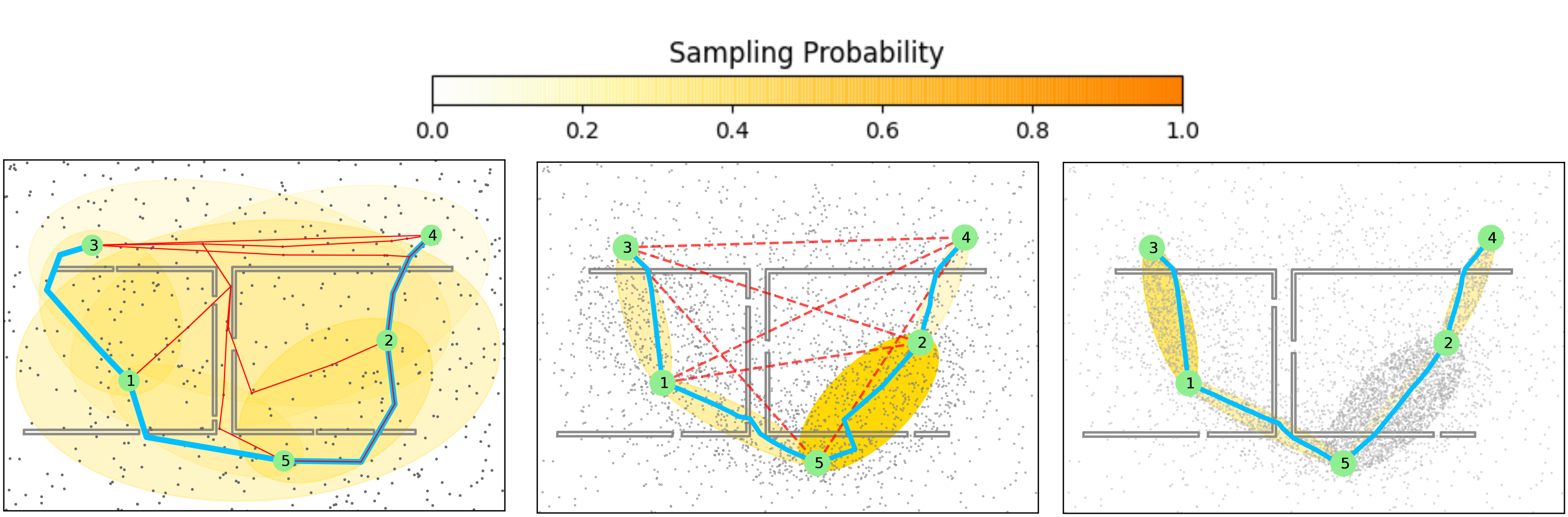
Figure 1: The Steiner tree (thick-blue lines) computed using a IST^*, showing the advantage of pruning. The environment has 2 U-shaped obstacles with tiny openings. Numbered nodes indicate terminals to be connected. Ellipses indicate an edge’s informed set, with color intensity related to sampling probability. Sampled points in free space are part of the roadmap (shown in grey). Left: without pruning, all non-MST edges (thin-red lines) are also sampled. Middle: with pruning, a subset of edges (dashed lines) may safely be removed without affecting the optimal MST. Right: after pruning, the roadmap is further densified around active edges that can lead to an optimal MST faster.

Irrespective of whether the search space is discrete or continuous, Steiner trees spanning the origin, goals and the destination play a critical role in the development of approximation algorithms for MGPF. In the discrete case, doubling the edges in a suitable Steiner tree, and finding a feasible path in the resulting Eulerian graph leads to 2-approximation algorithms for MGPF (Kou, Markowsky, and Berman 1981; Mehlhorn 1988; Chour, Rathinam, and Ravi 2021). This approach doesn’t readily extend to the continuous case because we do not a-priori know the travel cost between any two nodes in $T:=\{s,t\}\bigcup\bar{T}$. One can appeal to the well-known sampling-based methods (Karaman and Frazzoli 2011; Kavraki et al. 1996; Gammell, Srinivasa, and Barfoot 2014, 2015) to estimate the costs between the nodes, but the following key questions remain: 1) How to sample the space so that the costs of the edges joining the nodes in $T$ can be estimated quickly so that we can get a desired Steiner tree? 2) Should we estimate the cost of all the edges or can we ignore some edges and focus our effort on edges we think will likely end up in the Steiner tree?

We call our approach Informed Steiner Tree^∗ (IST^∗). IST^∗ iteratively alternates between sampling points in the search space and pruning edges. Throughout its execution, a Steiner tree is maintained which is initially empty but eventually spans the nodes in $T$, possibly including a subset of sampled points. IST* relies on two key ideas. First, finding a Steiner tree spanning $T$ commonly involves finding a Minimum Spanning Tree (MST) in the metric completion of the nodes in $T$. For any two distinct terminals $u,v$, we maintain a lower bound and an upper bound on the cost of the edge $(u,v)$. Using these bounds and cycle properties of an MST, we identify edges which will never be part of the MST. This allows us to only sample regions corresponding to the edges that are likely to be part of the MST. We further bias our sampling by assigning a suitable probability distribution over the search space based on the bounds on the cost of the edges (See Fig. 1). Second, as the algorithm progresses, a new set of points are added to the search graph in each iteration. Each new sample added may facilitate a lower-cost feasible path between terminals requiring us to frequently update the Steiner tree. To address this efficiently, we develop an incremental version of the Steiner tree algorithm while maintaining its properties. Since this incremental approach correctly finds a Steiner tree, as the number of sampled points tend the infinity, IST* provides an asymptotic 2-approximation guarantee for MGPF.

We use the sampling procedure developed in Informed RRT* (Gammell, Barfoot, and Srinivasa 2018) to choose points from selected regions in our approach. Informed sampling in synergy with pruning enables faster convergence to the optimal solution than uniform sampling. After describing IST^∗ with its theoretical properties, we provide extensive computational results on high-dimensional problem instances.

Related Work:

The MGPF and several variants of it have been addressed in the literature. Here, we discuss the most relevant work in continuous domains (more details are presented in the appendix). Un-supervised learning approaches(Faigl et al. 2011; Faigl 2016) using Self Organizing Maps (SOMs) have been used to solve MGPF. In (Faigl 2016), SOM is combined with a rapidly exploring random graph algorithm to find feasible solutions for the MGPF. In (Devaurs, Siméon, and Cortés 2014), a meta-heuristic similar to simulated annealing is combined with multiple Rapidly-exploring Random Tree (RRT) expansions to solve MGPF. In (Vonásek and Pěnička 2019), a method called Space Filling Forests (SFF) is proposed to solve MGPF. Multiple trees are grown from the nodes in $T$ and unlike the approach in (Devaurs, Siméon, and Cortés 2014) where any two close enough (or neighboring) trees are merged into a single tree, in SFF, multiple virtual connections are allowed between two neighboring trees leading to multiple paths between any two nodes in $T$. Recently, in (Janoš, Vonásek, and Pěnička 2021), a generalization of SFF (called SFF*) has been proposed to also include rewiring of the edges in the trees similar to RRT*. Computational results show that SFF* performed the best among several previously known solvers for the simulation environments considered in (Janoš, Vonásek, and Pěnička 2021). We evaluated SFF* on the environments we considered and report our findings in the results section.

A generalization of MGPF was considered in (Saha et al. 2006) where all the goals were partitioned into groups and the aim is to also visit one goal from each partition. They work under the assumption that a path between two nodes is computed at most once which may, in reality, be far from the optimal path. Their planner stops the instant it has found a feasible path connecting all the goals unlike our approach which keeps refining the paths.

Background and Preliminaries

Let $X\subseteq\mathbb{R}^{n}$ be the $n$-dimensional configuration spaceof a robot, and let $X_{f}\subset X$ be the set of obstacle-free configurations. Let $\sigma:[0,1]\rightarrow X_{f}$ be a collision free, feasible path such that the path starts at the origin ($\sigma(0)=s$), visits each of the goals in $\bar{T}$ at least once and ends at the destination ($\sigma(1)=d$). Let $c(\sigma)\in\mathbb{R}_{\geq 0}$ denote the cost of the path $\sigma$. The objective of MGPF is to find a collision-free feasible path $\sigma$ such that $c(\sigma)$ is minimized.

Let $S\subseteq X_{f}$ be a set of sampled points (also referred to as nodes) from $X_{f}$. Nodes which are within a radius of $\rho$ of each other are treated as neighbors. Edges are formed between neighbors if a feasible path is found between them using a local planner (for example, straight-line connection). Let $V:=S\bigcup{T}$. We refer to all the nodes in $T$ as terminals. Let $G=(V,E)$ denote the undirected graph thus formed where $E$ denotes all the edges joining any pair of neighbors in $V$. Henceforth, we refer to $G$ as the roadmap. Given a graph $G$, we use $E(G)$ to refer to all the edges present in $G$.

Let $e:=(u,v)$ be an edge joining two distinct nodes $u,v$ in $G$. Edge $e$ represents a feasible path between $u$ and $v$ found by the local planner. The cost of a feasible path joining vertices $u$ and $v$ is denoted as $dist(e)$. Let $h(e)$ be a lower bound on the length of any feasible path between $u$ and $v$; typically, we set $h(e)$ to be the Euclidean distance between the nodes $u$ and $v$.

One approach for solving the MGPF is to sample as many points uniformly as possible from the obstacle-free space and form a roadmap spanning the terminals and the sampled points. At the end of the search process, the recently developed $A^{*}$ based approach (Chour, Rathinam, and Ravi 2021) for discrete version of MGPF can be used to find a suitable Steiner tree. In this article, we consider this approach as the baseline against which IST^∗ is compared.

Informed Steiner Trees

1 Input:

$X_{f}\subset X$ // Collision free space

$T\subset X_{f}$ // Discrete set of terminals

$h(e)$ for any $e=(u,v),u,v\in X_{f}$ // Heuristic cost between terminals $u$ and $v$

$n_{s}$ // Samples per batch

$n_{b}$ // Number of batches

2 Output:

$S_{T}$ // Steiner tree spanning the terminals in $T$

3 Initialization:

$V\leftarrow T$ // Add terminals to the roadmap

$\mathcal{N}_{V}(u):=\{v:dist(v,u)\leq\rho,v\neq u,v\in V\}$ for any $u\in V$ // nearest neighbors of $u$ in $V$

4 $E\leftarrow\{(u,v):v\in\mathcal{N}_{V}(u),u\in V\}$

5 $cost(e)=dist(u,v)$ for any $e=(u,v)\in E$

6 $G\leftarrow(V,E)$

7

$\mathcal{A}=\{(u,v):u,v\in T,u\neq v\}$ // Set of active edges joining terminals

8 $cost_{T}(u,v)=\infty$ for any $(u,v)\in\mathcal{A}$

$Prob(e)=\frac{h(e)}{\sum_{e^{\prime}\in\mathcal{A}}h(e^{\prime})}$ for all $e\in\mathcal{A}$ // Initial probabilities using lower bounds

9 $S_{T}\leftarrow\emptyset$

10

// Note: $G,\bar{G},cost,cost_{T}$ are global variables.

11 Main loop:

12 for $iteration=1,\ldots,n_{b}$ do

13       $S^{\prime}\leftarrow AddSamples(Prob,\mathcal{A},cost_{T},n_{s})$

14      

15       $Ripple(S^{\prime})$

16      

17      $S_{T}\leftarrow UpdateTree(S_{T},\mathcal{A})$

18      

19       $\mathcal{A}\leftarrow PruneEdges(S_{T},\mathcal{A})$

20       $Prob\leftarrow UpdateProbability(Prob,\mathcal{A},S_{T},h)$

return $S_{T}$

Algorithm 1 IST^*

An overview of IST^* is presented in Algorithm 1. At any iteration, IST^* maintains three graphs to enable the search process:

1. Roadmap graph: $G=(V,E)$ includes all the terminals and the sampled points, and the edges between its neighboring nodes. Two nodes $u,v$ are neighboring if $dist(u,v)\leq\rho$, where $\rho$ is the connection radius. We provide a discussion on the role (and implementation) of $\rho$ in the Appendix. Initially, $G$ includes only the terminals and the edges between any pair of neighboring terminals.

2. Shortest-path graph: This graph is denoted as $\bar{G}:=(V,\bar{E})$ and is a subgraph of the roadmap. It is a forest which contains a tree corresponding to each terminal and maintains all the shortest paths from a terminal to each sampled point in its component. The shortest-path graph is used to find feasible paths between terminals. Initially, $\bar{G}$ is an empty forest ($i.e.$, contains no edges).

3. Terminal graph: This graph is denoted as $G_{T}=(T,\mathcal{A})$ and consists of only the terminals and any edges connecting them. Any edge in $G_{T}$ corresponds to a path between two terminals in the roadmap. Therefore, any spanning tree $S_{T}$ in the terminal graph corresponds to a feasible Steiner tree in $G$. It is used in determining which regions to sample and in finding feasible Steiner trees for MGPF. $\mathcal{A}$ contains the set of all the edges that can possibly be part of $S_{T}$, and hence are currently actively explored when sampling. Initially, $\mathcal{A}$ consists of all the edges that join any pair of terminals in $T$. As the algorithm progresses, edges in $\mathcal{A}$ may be pruned. Also, the cost of an edge connecting any pair of distinct terminals $u,v$ in $G_{T}$ is denoted as $cost_{T}(u,v)$. Initially, $cost_{T}(u,v)$ is set to $\infty$ for all $u,v\in T$ and $S_{T}$ is empty.

In each iteration of IST^*, the algorithm (i) samples new points in $X_{f}$ (line 21 of Algorithm 1), (ii) updates $S_{T}$ based on a new incremental Steiner tree algorithm called Ripple (lines 22–23 of Algorithm 1), (iii) prunes edges from $\mathcal{A}$ (line 24 of Algorithm 1), and (iv) updates the probability distribution (line 25 of Algorithm 1). Each of these key steps are discussed in the following subsections.

1 $S^{\prime}\leftarrow\emptyset$

2 for $1,\ldots,n_{s}$ do

3       Choose $(u,v)\in\mathcal{A}$ using $Prob$

4       $x_{rand}\leftarrow\texttt{Sample}(u,v,cost_{T}(u,v))$

5       $S^{\prime}\leftarrow S^{\prime}\cup\{x_{rand}\}$

6return $S^{\prime}$

Algorithm 2 AddSamples$(Prob,\mathcal{A},cost_{T},n_{s})$

// For any $u\in V$, let $r_{u}$ denote the closest terminal to $u$ in $G$. If $u$ is a terminal, then $r_{u}:=u$. The parent of any terminal is itself

1 while $S^{\prime}\neq\emptyset$ do

2       $s\leftarrow S^{\prime}.pop()$

3       $V\leftarrow V\cup\{s\}$

4       $E\leftarrow E\cup\{(s,u):u\in\mathcal{N}_{V}(s)\}$

5       $parent(s),r_{s}\leftarrow NULL$

6       $n^{*}=\arg\min\{g(n)+cost(s,n):n\in\mathcal{N}_{V}(s),r_{n}\neq NULL\}$

7       if $n^{*}\neq NULL$ then

8             $\bar{E}\leftarrow\bar{E}\cup\{(s,n^{*})\}$

9             $g(s)\leftarrow g(n^{*})+c(s,n^{*})$

10             $r_{s}\leftarrow r_{n^{*}}$

11             $parent(s)\leftarrow n^{*}$

12            

            $\mathcal{Q}.insert(s,g(s))$ // Priority Queue

13            

14            while $\mathcal{Q}\neq\emptyset$ do

15                   $u^{*}\leftarrow\mathcal{Q}.extractMin()$

16                   foreach $n\in N_{V}(u^{*})$ do

17                         if $g(u^{*})+cost(u^{*},n)<g(n)$ then

18                               $g(n)\leftarrow g(u^{*})+cost(u^{*},n)$

19                               $\mathcal{Q}.insert(n,g(n))$

20                               $r_{n}\leftarrow r_{u^{*}}$

21                               $\bar{E}\leftarrow\bar{E}\setminus\{(n,parent(n))\cup\{(n,u^{*})\}\}$

22                               $parent(n)\leftarrow u^{*}$

23                              

24                         else if $r_{n}\neq r_{u^{*}}$ then

25                               $d\leftarrow g(n)+cost(n,u^{*})+g(u^{*})$ if $d<cost_{T}(r_{n},r_{u^{*}})$ then

26                                     $cost_{T}(r_{n},r_{u^{*}})\leftarrow d$

27                                    

28                              

return

Algorithm 3 Ripple$(S^{\prime})$

// Notation: $\Omega((u,v),S_{T})$ is the cycle induced by adding edge $(u,v)$ to $S_{T}$

1 if $S_{T}$ is empty then

2       $S_{T}$ = Kruskal($cost_{T}$)

3       return $S_{T}$

4 for $(u,v)\in\mathcal{A}:(u,v)\not\in S_{T}$ do

5       $P:=\{(u^{\prime},v^{\prime})\in\Omega((u,v),S_{T})\setminus\{u,v\}\}$

6       $pathCost\leftarrow\sum\{cost_{T}(u^{\prime},v^{\prime}):(u^{\prime},v^{\prime})\in P\}$

7       $(u^{*},v^{*})=\arg\max\{cost_{T}(u^{\prime},v^{\prime}):(u^{\prime},v^{\prime})\in P\}\}$

8       if $cost_{T}(u^{*},v^{*})>cost_{T}(u,v)$ then

9             $S_{T}\leftarrow S_{T}\setminus\{(u^{*},v^{*})\}\cup\{(u,v)\}$

10       else if $pathCost<cost_{T}(u,v)$ then

             $cost_{T}(u,v)\leftarrow pathCost$ // Update non-MST edge with a cheaper path via MST

11            

12      

return $S_{T}$

Algorithm 4 UpdateTree$(S_{T},\mathcal{A})$

1 for $(u,v)\in\mathcal{A}:(u,v)\not\in S_{T}$ do

2       $(u^{*},v^{*})=\arg\max\{cost_{T}(u^{\prime},v^{\prime}):(u^{\prime},v^{\prime})\in\Omega((u,v),S_{T})\setminus\{u,v\}\}$

3       if $h(u,v)>cost_{T}(u^{*},v^{*})$ then

4             $\mathcal{A}\leftarrow\mathcal{A}\setminus\{(u,v)\}$

5      

return $\mathcal{A}$

Algorithm 5 PruneEdges$(S_{T},\mathcal{A})$

1

2if  $S_{T}$ is empty then

3       return $Prob$

// Reset probability distribution

4 $Prob(e):=0$ for all $e\in\{(u,v):u,v\in T,u\neq v\}$

5 $gap_{1}(e):=cost_{T}(u,v)-h(u,v),\forall(u,v)\in S_{T}$

6 $gap_{2}(e):=cost_{T}(u,v)-\max\{c(e^{\prime}):e^{\prime}\in\Omega(e,S_{T})\setminus\{e\}\},\forall e\in\mathcal{A}\setminus S_{T}$

// Partition active edges

7 $\mathcal{A}_{mst}=\{e\in S_{T}:gap_{1}(e)>0\}$

8 $\mathcal{A}_{non-mst}=\{e\in\mathcal{A}\setminus S_{T}:gap_{2}(e)>0\}$

9 foreach $e\in\mathcal{A}_{mst}$ do

10       $Prob(e)\leftarrow\frac{|\mathcal{A}_{mst}|}{|\mathcal{A}_{mst}|+|\mathcal{A}_{non-mst}|}\cdot\frac{gap_{1}(e)}{\sum_{e^{\prime}\in gap_{1}(e^{\prime})}}$

11foreach $e\in\mathcal{A}_{non-mst}$ do

12       $Prob(e)\leftarrow\frac{|\mathcal{A}_{non-mst}|}{|\mathcal{A}_{mst}|+|\mathcal{A}_{non-mst}|}\cdot\frac{gap_{2}(e)}{\sum_{e^{\prime}\in gap_{2}(e^{\prime})}}$

return $Prob$

Algorithm 6 UpdateProbability$(Prob,\mathcal{A},S_{T},h)$

Sampling:

The sampling procedure (Algorithm 2) uses the routine Sample developed in Informed RRT* (Gammell, Srinivasa, and Barfoot 2014, Algorithm 2). In this procedure, a fixed number of samples $n_{s}$ is added to $S^{\prime}$ from $X_{f}$ in each iteration. First, an edge $e:=(u,v)$ is drawn from the probability distribution over $\mathcal{A}$ (line 3 in Algorithm 2). Initially, until a feasible $S_{T}$ is obtained, the probability distribution is computed using the heuristic lower bounds (line 1 in Algorithm 1). Once a random sample $x_{rand}$ is obtained for the edge $(u,v)$ using Sample, it is added to $S^{\prime}$.

Incremental Steiner tree algorithm:

This procedure is accomplished by first finding lower-cost, feasible paths between the terminals through Ripple (Algorithm 3), and then updating the spanning tree $S_{T}$. In Ripple, each sample is processed individually until $S^{\prime}$ becomes empty. Adding a new point $s$ to the roadmap (consequently to $\bar{G}$) can facilitate new paths between terminals. If $s$ has a neighbor that is connected to a terminal (or is itself a terminal), then $s$ and each of its neighbors are expanded in a Dijkstra-like fashion until the priority queue $\mathcal{Q}$ is empty (lines 3–3 of Algorithm 3). The variable $g(u)$ keeps track of the shortest path from $u$ to its closest terminal which is stored in $r_{u}$. The key part of the Ripple algorithm lies in finding new feasible paths between the terminals. This happens (line 3 of Algorithm 3) during the expansion of a node $u^{*}$ to its neighbor $n$ when $g(u^{*})+cost(u^{*},n)\geq g(n)$ and $r_{u^{*}}\neq r_{u}$, $i.e.$, $n$ is closer to its root $r_{n}$ than to $r_{u^{*}}$. In this case, a feasible path from $r_{u^{*}}$ to $r_{n}$ has been discovered through the nodes $u^{*}$ and $n$. If the cost of this feasible path is lower than $cost_{T}(r_{u^{*}},r_{n})$, then $cost_{T}(r_{u^{*}},r_{n})$ is updated accordingly.

After $cost_{T}(u,v)$ for any pair of terminals $(u,v)$ is updated, it is relatively straightforward to check if any edge not in $S_{T}$ should become part of $S_{T}$. First, we check if $S_{T}$ is empty or not. If $S_{T}$ is empty, then we just use the Kruskal’s algorithm (Kruskal 1956) to find a spanning tree (if it exists) for $T$ (line 2 of Algorithm 4). If $S_{T}$ is not empty, we appeal to the following well-known cycle property of minimum spanning trees to see if we should include $(u,v)$ in $S_{T}$.

Cycle Property.

Suppose that $S_{T}$ is a MST in $G_{T}$ and when a new edge $(u,v)\notin S_{T}$ is added to $G_{T}$, it forms a cycle $C=\Omega((u,v),S_{T})$. Consider an edge $(u^{*},v^{*})\in C$ other than $(u,v)$ that has the maximum of all the edge costs in $C$. If $cost_{T}(u^{*},v^{*})>cost_{T}(u,v)$, then $S_{T}\setminus\{(u^{*},v^{*})\}\cup\{(u,v)\}$ is an MST of the updated $G_{T}$.

Thus, in our algorithm, if $cost_{T}(u^{*},v^{*})>cost_{T}(u,v)$, then edge $(u^{*},v^{*})$ is deleted from $S_{T}$ and edge $(u,v)$ is added to $S_{T}$ (lines 9 of Algorithm 4).

Pruning edges from $\mathcal{A}$:

The pruning procedure (Algorithm 5) is similar to what we discussed in the previous tree update procedure except that we now appeal to the bounds on the cost of the edges. Consider an edge $(u^{*},v^{*})\in\Omega((u,v),S_{T})$ other than $(u,v)$ that has the maximum of all the edge costs in $C$. If $cost_{T}(u^{*},v^{*})<h(u,v)$, and since $h(u,v)\leq cost_{T}(u,v)$, we have $cost_{T}(u^{*},v^{*})<cost_{T}(u,v)$. Then, again applying the cycle property, edge $(u,v)$ is pruned from $\mathcal{A}$ and is never considered by the algorithm henceforth (line 4 of Algorithm 5).

Update probability distributions:

Once a feasible $S_{T}$ is found, the probability distribution is updated (Algorithm 6) in each iteration to reflect the changes in the costs and $\mathcal{A}$. We want to sample the region around an edge more if the uncertainty around the cost of the edge is higher. This is based on our assumption that the more we learn about the cost of an edge, the better we can decide on its inclusion in $S_{T}$. If an edge $(u,v)$ already belongs to $S_{T}$, we assign a sampling probability for $(u,v)$ proportional to the difference between the edge cost and its lower bound. On the other hand, if an edge $(u,v)$ does not belong to $S_{T}$, we first aim to include it in $S_{T}$ and later hope to drive its cost to its lower bound. Thus, we assign a sampling probability for $(u,v)$ proportional to the difference between the edge cost and the cost of its next largest cost edge in $\Omega((u,v),S_{T})$.

Theoretical Properties

At any iteration of the algorithm, the algorithm maintains a Steiner tree $S_{T}$ which is formed by expanding the paths of a MST on the terminal graph $G_{T}$. For any given state of the graph $G$ that contains the terminals $T$ along with the sampled points so far, we argue that the tree returned by IST^* is such an MST.

Theorem 1.

IST^* will return an MST over the shortest paths between terminals in $G$.

We show this theorem by arguing that the edge pruning from the active set $\cal A$ of inter-terminal edges is correct and that the sampling procedure with updated probabilities coupled with the Ripple update will eventually find all relevant shortest paths. The former claim follows from the cycle property as discussed in the pruning step. To prove the latter claim, we use the following key lemma, that is proved in the Appendix.

Lemma 2.

Suppose a sample point $s\in S^{\prime}$ is processed by Ripple so that $r_{s}$ is a terminal $t$, then in $G$, $t$ is (one of) the closest terminal to $s$ among all terminals $T$.

In this way, Ripple maintains every sample point in the correct so-called ‘Voronoi’ partition of the terminals (i.e. assigning it to its closest terminal). From this lemma, we see that the edges between terminals in $G_{T}$ whose costs are updated by Ripple (line 24, Algorithm 3) are precisely those where an edge between a node $u^{*}$ and its neighbor $n$ such that $r_{u^{*}}\neq r_{n}$ discovers a new cheaper path between $r_{u^{*}}$ and $r_{n}$. Thus, Ripple is able to find all shortest paths between pairs of terminals that are witnessed by a pair of neighboring boundary We can now use a result of (Mehlhorn 1988) (Lemma in Section 2.2) that shows that this subgraph $G_{T}$ of the subset of shortest paths between terminals in $T$ that are witnessed by adjacent boundary nodes is sufficient to reconstruct an MST of $G$. This shows that $S_{T}$ constructed as a MST of $G_{T}$ is indeed an MST of the metric completion of $T$ using all the edges in $G$ as claimed.

Since the UpdateTree method in IST^* always maintains a MST of the sampled graph $G$, in the limit with more sampling, the actual shortest paths corresponding to the true final MST will be updated to their correct lengths with diminishing error, and this MST will be output by IST^*. Since the MST is a 2-approximation to the optimal Steiner tree in any graph and consequently, the MGPF problem (Kou, Markowsky, and Berman 1981), we get the following result.

Corollary 3.

IST^* outputs a 2-approximation to the MGPF problem asymptotically.

Results

Env.	10 Terminals	30 Terminals	50 Terminals
CO $\mathbb{R}^{4}$
CO $\mathbb{R}^{8}$
UH $\mathbb{R}^{4}$
UH $\mathbb{R}^{8}$
H O M E
A B S T R A C T

Table 1: Comparison of IST^* against the Baseline across 6 different environments – real vector spaces over uniform hyper rectangles (UH) and center obstacles CO, and $SE(3)$ environments HOME and ABSTRACT – over 10/30/50 terminals. The thin solid line represents the mean solution cost with the shaded region being the 99% confidence interval about this mean.

Env.	10 Terminals	30 Terminals	50 Terminals
H O M E
UH $\mathbb{R}^{8}$

Table 2: Comparison of the performance of IST^* when Ripple is used against S* on an $SE(3)$ instance ($Home$) and a high-dimensional environment (UH $\mathbb{R}^{8}$). The dark line represents the mean solution cost with the thick region being the 99% confidence interval about the mean.

To evaluate the performance of IST^*, we compared it with a baseline as described in the Background and Preliminaries section. Specifically for the baseline, we densified a roadmap given by PRM^* (Karaman and Frazzoli 2011) for a fixed amount of time via uniform random sampling after which S^* (S^*-BS variant was used) was run on the resulting roadmap to obtain an MST-based Steiner tree (Chour, Rathinam, and Ravi 2021). It was ensured that the combined time spent in growing the roadmap and running S^* exhausted the input time limit.

The planners (IST^* and the Baseline) were implemented in Python 3.7 using OMPL (Şucan, Moll, and Kavraki 2012) v1.5.2 on a desktop computer running Ubuntu 20.04, with 32 GB of RAM and an Intel i7-8700k processor. Further implementation details are available in the Appendix. Both the planners output the cost of the Steiner tree found over time. Each planner was ran 50 times to obtain a distribution of solution costs. The mean solution cost with a 99% confidence interval is calculated from 50 trials and shown in Table 1.

Table 3: Time (in seconds) given to planners as input in different problem instances.

$$\begin{array}[]{|c|c|c|c|}\hline\cr\leavevmode\hbox to104.89pt{\vbox to18.98pt{\text{[drawing]}}}&10&30&50\\ \hline\cr\texttt{CO}\ \ \mathbb{R}^{4}&450s&900s&1350s\\ \hline\cr\texttt{CO}\ \ \mathbb{R}^{8}&900s&1800s&2700s\\ \hline\cr\texttt{UH}\ \ \mathbb{R}^{4}&600s&1200s&1800s\\ \hline\cr\texttt{UH}\ \ \mathbb{R}^{8}&1200s&2400s&3600s\\ \hline\cr HOME&600s&1200s&1800s\\ \hline\cr ABSTRACT&600s&600s&600s\\ \hline\cr\end{array}$$

Due to the absence of a standard suite of instances for benchmarking planners for MGPF, we use the environments commonly considered in motion planning and extend them to our setting by randomly generating valid goal configurations. Specifically, we test our planners in high-dimensional state spaces, and on rigid body motion planning instances available in the OMPL.app GUI. A problem instance is uniquely identified by an environment (with its specific robot model), number of terminals, and the computational time given for planning. For each environment, a varying number of terminals ($|T|=10,30,50$) was generated. The choice for the size of the problem instances was motivated by unmanned vehicle applications (Oberlin, Rathinam, and Darbha 2011). The time specified in problem instances was based on the number of terminals and the difficulty of planning in that environment (Table 3). We now describe the testing environments and the corresponding results.

Real-vector space problems

IST^* and the Baseline were tested on two simulated problems in a unit hypercube with distinct obstacle configurations in $\mathbb{R}^{4}$ and $\mathbb{R}^{8}$ (Fig. 2). The collision detection resolution was set to $10^{-4}$ to make evaluating edge costs computationally expensive.

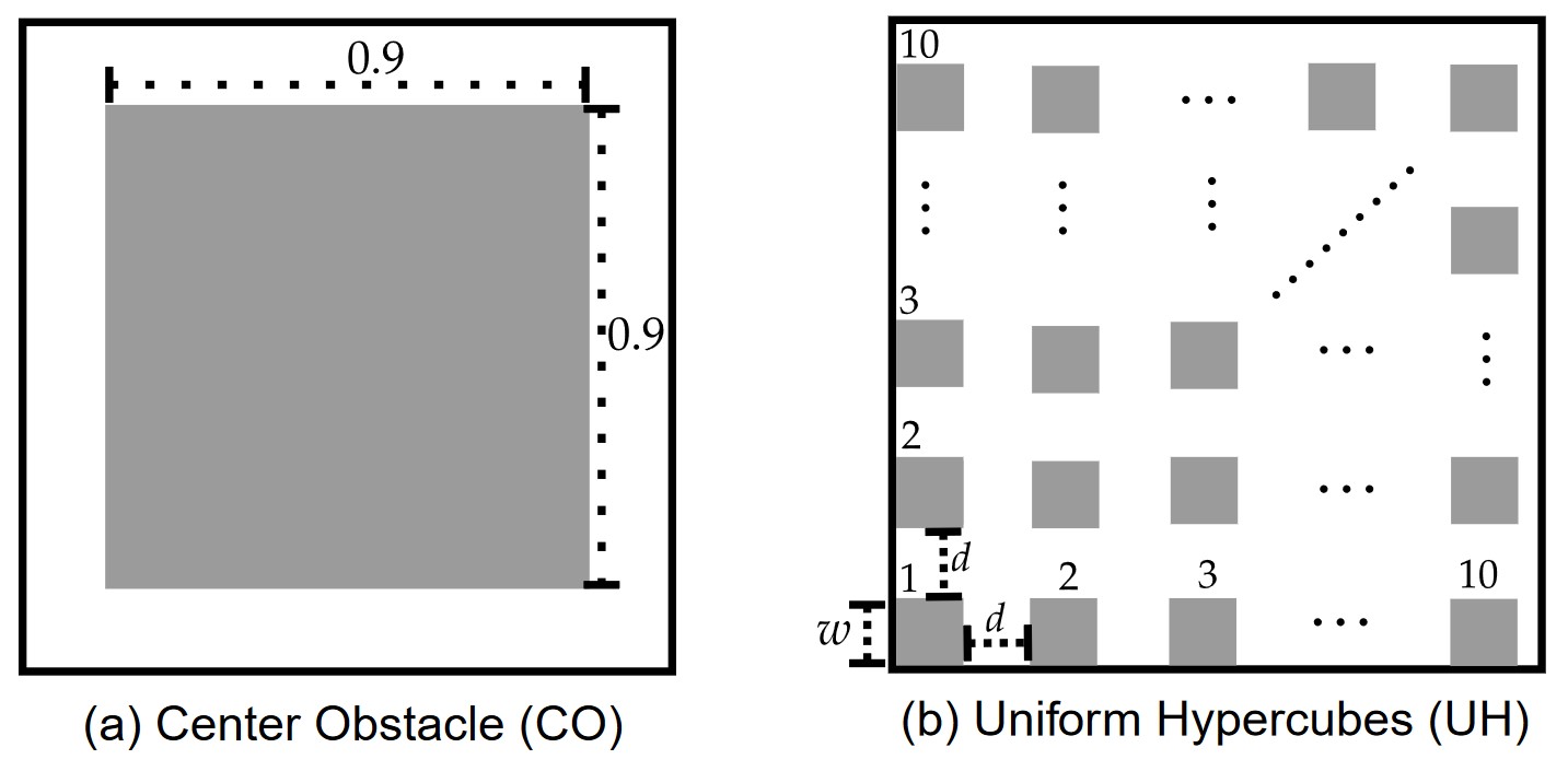
Figure 2: A 2-dimensional illustration of the problems in real-vector spaces. The configuration space for both is a unit hypercube, $i.e.$, each state space was bounded to the interval [0, 1], illustrated by the black bounding box. Solid regions represent invalid states. In Fig.2(b), the hypercube obstacles are axis-aligned (specifically, 10 on each axis) and uniformly spread with $w=0.075,d=0.025$.

Center Obstacle (CH): This problem consisted of a big hypercube at the center (with volume $(0.9)^{n}$ in $\mathbb{R}^{n}$) (Fig. 2a). In this environment, IST^* started on par with the Baseline but significantly improved while the Baseline remained stuck in a sub-optimal solution.

Uniform Hypercubes (UH): This domain was filled with a regular pattern of axis-aligned hypercubes (identically distributed with uniform gaps) (Fig. 2b). For a real vector space of dimension $n$, this environment contains $10^{n}$ obstacles with a total volume of $0.75^{n}$. In this environment, we see a dominant performance of IST* over the Baseline with up to $30\%$ better solution cost.

$\mathbf{SE(3)}$ problems

As the environment models in OMPL App are designed for single source and destination motion planning (with no goals), many of them have disconnected regions making them unsuitable for benchmarking multi-goal path planning under random generation of goal points. Thus, we used the $Home$ and $Abstract$ environment which not only admit one connected $SE(3)$ configuration space but also offer several homotopy classes of solution paths.

$Home$ and $Abstract$ environments are related to the classic Piano Mover’s problem, admitting several narrow passages. $Home$ offers the highest scope for optimization among all the environments considered, with the final solution often being $50\%$ better than the initial solution. In $Home$, Baseline performs competitively to IST^*, and sometimes also finds better solutions initially. However, IST^* converges to a better solution asymptotically in all the problem instances of $Home$. In $Abstract$, both Baseline and IST* find a good solution quickly, and as a result, the scope for optimization is not much. Still, IST* is able to improve very quickly, dominates throughout, and reaches the final solution cost of Baseline $\approx 6$ times faster.

Impact of Ripple

In each iteration of IST^*, a batch of samples is added to the roadmap $G$. As Ripple processes each sample incrementally and keeps rewiring a rooted shortest-path tree until convergence, it may seem better to simply add all the samples at once and then run S* on the updated roadmap to get $S_{T}$. However, the roadmap grows significantly over time, making S* computationally expensive for repeated executions. Whereas, Ripple only has to process a small fraction of the roadmap for a fixed number of samples per batch.

We benchmarked Ripple with S* to investigate its effect on the performance of IST^*. A pseudorandom generator was used for generating the same sample points for both. The problem instances considered for this comparison were same as before (Table 3). However, due to space constraints, we only show the results (in Table 2) for just $2$ environments depicting extreme scenarios. In UH  $\mathbb{R}^{8}$, both S* and Ripple perform similarly, with Ripple being marginally better in the instance with $50$ terminals. In $Home$, Ripple not only finds a better final solution, but is also $2-3$x faster than S* for the same solution cost consistently. In all other problem instances as well, these 2 scenarios were observed throughout: either Ripple’s performance was very similar to S* or it was significantly faster while converging to a better solution. In conclusion, while both S* and Ripple can lead to the optimal MST over $G_{T}$, Ripple dominates S* across all instances considered.

Comparison with SFF^*

SFF^* (Janoš, Vonásek, and Pěnička 2021) is an algorithm that builds multiple RRTs to find distances between terminals and is designed to terminate when all target locations have been connected to a single component. The performance of SFF^* is not shown in the experimental plots for the following reasons: 1) The available implementation of SFF^* only supports $SE(3)$ (and its subspace), and thus cannot be evaluated on environments like $\mathbb{R}^{4}$ and $\mathbb{R}^{8}$ presently. 2) We benchmarked SFF^* on $Home$ and $Abstract$ but we encountered long termination times.

Comparing Path Costs

While IST^*’s primary output is a Steiner tree, we also evaluated the cost of the feasible path obtainable from IST^* for MGPF. Overall, it was seen to perform better than the Baseline in path computations too, an example of which is shown on two challenging problem instances in Fig. 3.

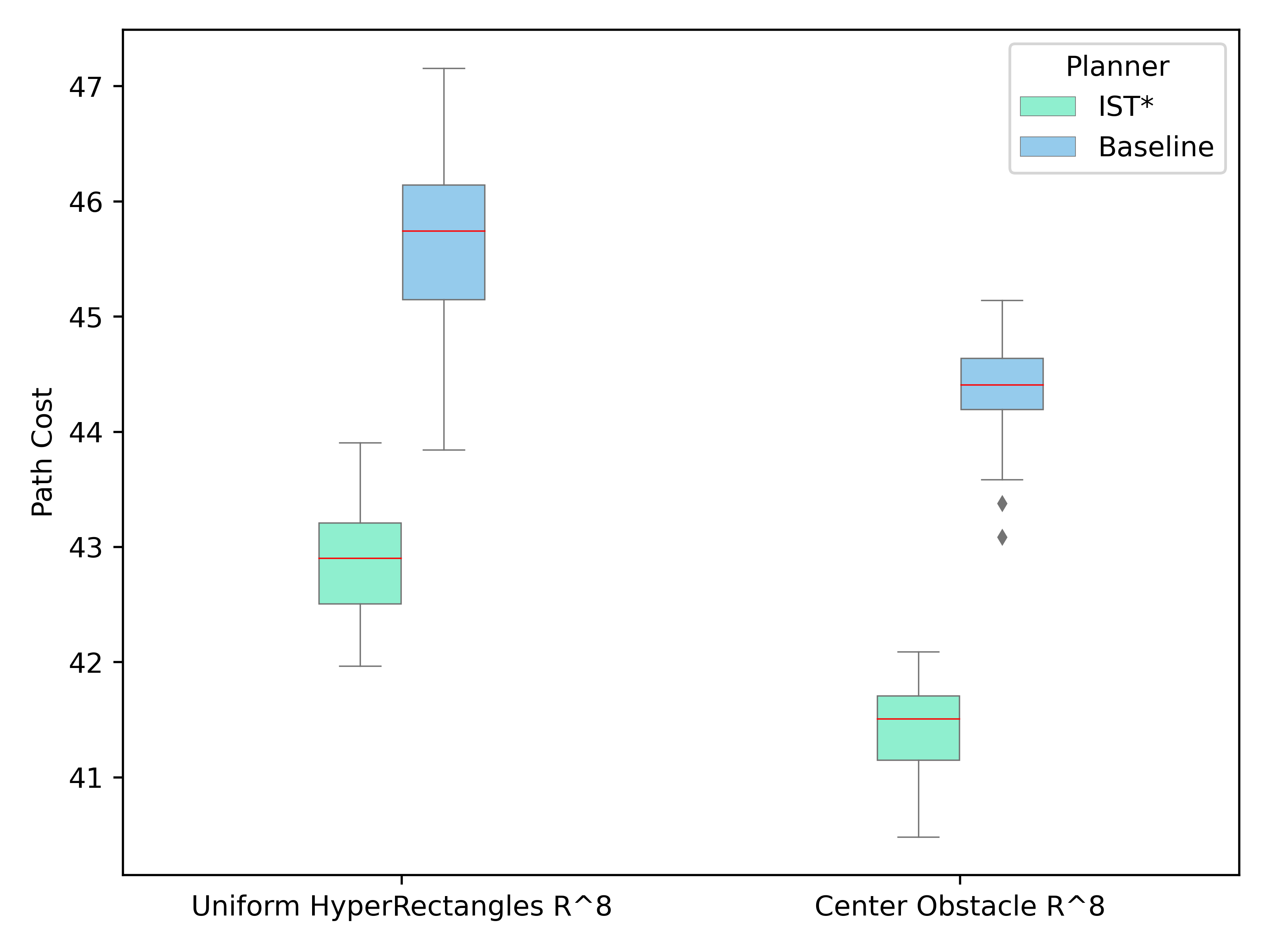
Figure 3: Comparisons of the costs of the feasible MGPF solution found by the planners in the high-dimensional real environments with 50 terminals (over 50 runs).

Conclusion

Inspired by the recent advancements in sampling-based methods for shortest path problems for single source and destination in continuous space and multi-goal path finding in discrete space, we provide a unifying framework to promote a novel line of research in MGPF. For the first time, to the best of the authors’ knowledge, the ideas of informed sampling have been fruitfully extended to the setting of planning for multiple goals. Our approach is decoupled in the sense that any further advancements in PRM* or informed sampling can be directly used to update the respective components of our proposed framework.

In the future, we plan to explore obtaining effective lower bounds on the shortest path cost between two terminals instead of using the Euclidean distance. Including heuristics in Ripple also seems to be a promising line of research.

References

- Best, Faigl, and Fitch (2016) Best, G.; Faigl, J.; and Fitch, R. 2016. Multi-robot path planning for budgeted active perception with self-organising maps. In 2016 IEEE/RSJ International Conference on Intelligent Robots and Systems (IROS), 3164–3171. IEEE.
- Chour, Rathinam, and Ravi (2021) Chour, K.; Rathinam, S.; and Ravi, R. 2021. S*: A Heuristic Information-Based Approximation Framework for Multi-Goal Path Finding. In Proceedings of the International Conference on Automated Planning and Scheduling, volume 31, 85–93.
- Devaurs, Siméon, and Cortés (2014) Devaurs, D.; Siméon, T.; and Cortés, J. 2014. A multi-tree extension of the Transition-based RRT: Application to ordering-and-pathfinding problems in continuous cost spaces. In 2014 IEEE/RSJ International Conference on Intelligent Robots and Systems, 2991–2996. IEEE.
- Edelkamp, Secim, and Plaku (2017) Edelkamp, S.; Secim, B. C.; and Plaku, E. 2017. Surface inspection via hitting sets and multi-goal motion planning. In Annual Conference Towards Autonomous Robotic Systems, 134–149. Springer.
- Faigl (2016) Faigl, J. 2016. On self-organizing map and rapidly-exploring random graph in multi-goal planning. In Advances in self-organizing maps and learning vector quantization, 143–153. Springer.
- Faigl et al. (2011) Faigl, J.; Kulich, M.; Vonásek, V.; and Přeučil, L. 2011. An application of the self-organizing map in the non-Euclidean Traveling Salesman Problem. Neurocomputing, 74(5): 671–679.
- Gammell, Barfoot, and Srinivasa (2018) Gammell, J. D.; Barfoot, T. D.; and Srinivasa, S. S. 2018. Informed sampling for asymptotically optimal path planning. IEEE Transactions on Robotics, 34(4): 966–984.
- Gammell, Srinivasa, and Barfoot (2014) Gammell, J. D.; Srinivasa, S. S.; and Barfoot, T. D. 2014. Informed RRT*: Optimal sampling-based path planning focused via direct sampling of an admissible ellipsoidal heuristic. In 2014 IEEE/RSJ International Conference on Intelligent Robots and Systems, 2997–3004. IEEE.
- Gammell, Srinivasa, and Barfoot (2015) Gammell, J. D.; Srinivasa, S. S.; and Barfoot, T. D. 2015. Batch informed trees (BIT*): Sampling-based optimal planning via the heuristically guided search of implicit random geometric graphs. In 2015 IEEE international conference on robotics and automation (ICRA), 3067–3074. IEEE.
- Janoš, Vonásek, and Pěnička (2021) Janoš, J.; Vonásek, V.; and Pěnička, R. 2021. Multi-goal path planning using multiple random trees. IEEE Robotics and Automation Letters, 6(2): 4201–4208.
- Karaman and Frazzoli (2011) Karaman, S.; and Frazzoli, E. 2011. Sampling-based algorithms for optimal motion planning. The international journal of robotics research, 30(7): 846–894.
- Kavraki et al. (1996) Kavraki, L.; Svestka, P.; Latombe, J.-C.; and Overmars, M. 1996. Probabilistic roadmaps for path planning in high-dimensional configuration spaces. IEEE Transactions on Robotics and Automation, 12(4): 566–580.
- Kou, Markowsky, and Berman (1981) Kou, L.; Markowsky, G.; and Berman, L. 1981. A fast algorithm for Steiner trees. Acta Informatica, 15(2): 141–145.
- Kruskal (1956) Kruskal, J. B. 1956. On the shortest spanning subtree of a graph and the traveling salesman problem. Proceedings of the American Mathematical society, 7(1): 48–50.
- Kuffner and LaValle (2000) Kuffner, J.; and LaValle, S. 2000. RRT-connect: An efficient approach to single-query path planning. In Proceedings 2000 ICRA. Millennium Conference. IEEE International Conference on Robotics and Automation. Symposia Proceedings (Cat. No.00CH37065), volume 2, 995–1001 vol.2.
- Macharet and Campos (2018) Macharet, D. G.; and Campos, M. F. 2018. A survey on routing problems and robotic systems. Robotica, 36(12): 1781–1803.
- McMahon and Plaku (2015) McMahon, J.; and Plaku, E. 2015. Autonomous underwater vehicle mine countermeasures mission planning via the physical traveling salesman problem. In OCEANS 2015-MTS/IEEE Washington, 1–5. IEEE.
- Mehlhorn (1988) Mehlhorn, K. 1988. A faster approximation algorithm for the Steiner problem in graphs. Information Processing Letters, 27(3): 125–128.
- Oberlin, Rathinam, and Darbha (2011) Oberlin, P.; Rathinam, S.; and Darbha, S. 2011. Today’s Traveling Salesman Problem. Robotics and Automation Magazine, IEEE, 17: 70 – 77.
- Otto et al. (2018) Otto, A.; Agatz, N.; Campbell, J.; Golden, B.; and Pesch, E. 2018. Optimization approaches for civil applications of unmanned aerial vehicles (UAVs) or aerial drones: A survey. Networks, 72(4): 411–458.
- Saha et al. (2006) Saha, M.; Roughgarden, T.; Latombe, J.-C.; and Sánchez-Ante, G. 2006. Planning tours of robotic arms among partitioned goals. The International Journal of Robotics Research, 25(3): 207–223.
- Şucan, Moll, and Kavraki (2012) Şucan, I. A.; Moll, M.; and Kavraki, L. E. 2012. The Open Motion Planning Library. IEEE Robotics and Automation Magazine, 19(4): 72–82. https://ompl.kavrakilab.org.
- Vonásek and Pěnička (2019) Vonásek, V.; and Pěnička, R. 2019. Space-filling forest for multi-goal path planning. In 2019 24th IEEE International Conference on Emerging Technologies and Factory Automation (ETFA), 1587–1590. IEEE.