A Probabilistic Generative Model of Free Categories

Abstract

Applied category theory has recently developed libraries for computing with morphisms in interesting categories, while machine learning has developed ways of learning programs in interesting languages. Taking the analogy between categories and languages seriously, this paper defines a probabilistic generative model of morphisms in free monoidal categories over domain-specific generating objects and morphisms. The paper shows how acyclic directed wiring diagrams can model specifications for morphisms, which the model can use to generate morphisms. Amortized variational inference in the generative model then enables learning of parameters (by maximum likelihood) and inference of latent variables (by Bayesian inversion). A concrete experiment shows that the free category prior achieves competitive reconstruction performance on the Omniglot dataset.

1 Introduction

Applied category theory has recently developed software libraries for representing and computing with morphisms in various categories, with a particular focus on (symmetric) monoidal categories and diagrammatic reasoning (e.g. [17, 29, 54, 53]). Categories have also emerged as a common representation for computer programs in different languages [65, 14]. In parallel, the field has worked to provide categorical semantics and interpretations for a variety of machine learning (ML) and artificial intelligence (AI) building blocks, including neural networks [18, 19, 11], and probabilistic inference [25, 12, 7, 22].

The intersection of learning and compositional reasoning has challenged the cognitive sciences (AI, ML, cognitive science, etc.) from the beginning. Theoretical arguments suggest that a generally intelligent agent ought to reason compositionally [55, 43], to employ something like computable programs as models of the world [64], and to prefer simpler programs to more complex ones [69]. Evidence from a variety of experiments [39, 35, 27, 38, 74] suggests that abductive learning of program-like causal models provides a domain-general foundation for human intelligence.

Most process models of cognition spring from a limited selection of metaphors for how the mind works. For instance, cognitive scientists continue to debate whether the mind builds concepts by means of a “language of thought” [56, 51, 58] or convex geometric spaces [23]. Some cognitive neuroscientists find tentative support for both “map-like” and “sentence-like” processes in the brain [21] while others argue for a more connectionist “direct fit” [30]. Machine learning scientists tackling the learning and synthesis of task-specific policies or programs tend to employ either Bayesian inference over a context-free grammar of programs, reinforcement learning of neural network policies, or both [52, 68, 50].

Category theory readers will notice that program learning tasks, via their context-free grammars, work with the compositional structure of operads [32, 20]. The connection suggests that categories, too, could provide a setting for learning and inference. This paper thus suggests an additional alternative to the options of neural networks and grammatical programs: a probabilistic generative model (PGM) of morphisms in a free monoidal category. This free category prior is parameterized by generating objects and morphisms (to construct the free category) and wiring diagrams (to sample specific morphisms). An experiment shows that the model’s software implementation can learn to compose deep generative models to achieve competitive performance in reconstruction evaluation data.

Outline

Section 2 summarizes the categorical background for the rest of the paper: our chosen setting for categorical probability in Section 2.1, and the operad of wiring diagrams for use as specifications in Section 2.2. Section 3 then defines the necessary categorical machinery for generative modeling, presents the free category prior, and demonstrates its basic properties. Section 4 describes its software implementation, describes amortized variational inference (Section 4.2), and presents a basic experiment (Section 4.3) showing that fitting the free category model to data yields competitive performance in a generative modeling task. Section 5 discusses extensions and further applications.

2 Categorical background

2.1 Markov categories

In this paper we build upon Markov categories, a formalism presented by Fritz [22] following a series of works by Golubtsov [26] and Cho and Jacobs [7]. It allows us to represent fundamental concepts from probability theory (such as conditioning, causality, almost surety, etc.) in purely categorical terms. In particular we work in QBS (i.e., the category of quasi-Borel spaces) by Heunen et al. [33]. In the following we use the notation $\fatsemi$ and $\odot$ throughout for sequential and monoidal composition.

Definition 1 (Markov Category).

A Markov category $\mathcal{C}$ is a symmetric monoidal category in which every object $X\in\mathcal{C}$ is equipped with a commutative comonoid structure given by a comultiplication $\textbf{copy}_{\_}X:X\rightarrow X\odot X$ and a counit $\textbf{del}_{\_}X:X\rightarrow I$.

Modeling probability theory in a Markov category involves the following steps:

• Identify a base Markov category $\mathcal{C}$ (usually a category of certain type of measurable spaces).

• Identify a monad (usually Giry/probability monad) represented by an endofunctor $\mathbb{P}\>:\mathcal{C}\rightarrow\mathcal{C}$.

• Take the Kleisli category $Kl(\mathbb{P}\>)$ of the monad $\mathbb{P}\>$.

Corollary 3.2 in [22] says that if $\mathbb{P}\>$ is a symmetric monoidal affine monad then the Kleisli category $Kl(\mathbb{P}\>)$ is again a Markov category. In particular, the Giry monad is symmetric monoidal and affine.

Typically Markov categories consist of certain measurable spaces as objects and Markov kernels as morphisms. In QBS, by contrast, each object consists of a pair of a sample space $X$ and a collection of $X$-valued random variables $M_{\_}{X}\subseteq[\mathbb{R}\rightarrow X]$ (which must be closed under certain conditions) and the morphisms are random functions between sample spaces that extend the random variables in the domain to random variables in the codomain. Random variables are thus fundamental, rather than being derived from a $\sigma$-algebra of measurable subsets. They then derive their randomness from probability measures in $\mathbb{R}$, as we will discuss below.

Definition 2 (Category of quasi-Borel spaces).

A quasi-Borel space is a set $X$, which we call the sample space, together with a set of functions $M_{\_}X\subseteq[\mathbb{R}\rightarrow X]$ that

• Contains all constant functions: $\alpha\in M_{\_}{X}$ if $\alpha:\mathbb{R}\rightarrow X$ is constant;

• Is closed under pre-composition: $\alpha\circ f\in M_{\_}{X}$ if $\alpha\in M_{\_}X$ and $f:\mathbb{R}\rightarrow\mathbb{R}$ is measurable; and

• Is closed under countable mixtures: with respect to a partition of $\mathbb{R}$ into a disjoint union of countably many Borel sets i.e. $\mathbb{R}=\biguplus_{\_}{i\in\mathbb{N}}S_{\_}{i}$, and $\alpha_{\_}{1},\alpha_{\_}{2},\ldots\in M_{\_}{X}$ then the mixed random variable $\beta$ is in $M_{\_}{X}$ where $\beta(r)=\alpha_{\_}i(r)$ for $r\in S_{\_}i$.

Morphisms $(X,M_{\_}X)\rightarrow(Y,M_{\_}Y)$ between quasi-Borel spaces consist of functions $f:X\rightarrow Y$ such that $f\circ\alpha\in M_{\_}Y$ for all $\alpha\in M_{\_}X$.

Together these form the category of Quasi-Borel Spaces and measurable functions between them (QBS), with function composition as composition of morphisms and identity functions as identity morphisms.

To study probability theory via quasi-Borel spaces, there is a notion of probability measure on them.

Definition 3 (Probability measure on quasi-Borel space.).

A probability measure on a quasi-Borel space $(X,M_{\_}X)$ is a pair $(\alpha,\mu)$ where $\alpha\in M_{\_}X$ and $\mu$ is a probability measure on $\mathbb{R}$. Here $\mu$ is a probability measure from the standard measure theory.

The above definition reflects the usual notion of a probability measure on a measurable space which is induced via pushing-forward through a random variable (a measurable function) from the sample space with a probability measure. Another way of phrasing the notion of probability measure is that with a source of randomness from $\mathbb{R}$ and a distribution $\mu$ on $\mathbb{R}$, we observe the effect of the process $\alpha\in M_{\_}X$ in $X$. From this notion of probability measure, there is generalized version of Giry monad in QBS which is referred as the probability monad.

Lemma 1 (Probability monad in QBS, due to Heunen et al. [33]).

The set of all probability measures on a quasi-Borel space naturally forms a quasi-Borel space (see Heunen et al. [33]). The endofunctor $\mathbb{P}\>$ sending a quasi-Borel $X$ to the space $\mathbb{P}\>X$ of probability measures on $X$ (quotienting out a suitable notion of equivalent measures) gives rise to a commutative monad in QBS with Kleisli composition $\fatsemi_{\_}{\mathbb{P}\>}:\mathbf{QBS}(A,\mathbb{P}\>B)\times\mathbf{QBS}(B,\mathbb{P}\>C)\rightarrow\mathbf{QBS}(A,\mathbb{P}\>C)$ and unit natural transformation $\eta:\mathbb{I}\rightarrow\mathbb{P}\>$ from the identity functor $\mathbb{I}$.

2.2 Wiring diagram operads and algebras over them

Rupel and Spivak [60] introduced wiring diagrams as a formal graphical language to represent the structure of composite processes. Despite their geometric presentation, wiring diagrams should be understood as combinatorial entities. Every wiring diagram is a combinatorial scheme of composing blank boxes and directed wires, and Patterson et al. [54] showed that wiring diagrams provide a combinatorial normal form for morphisms in SMCs. This makes wiring diagrams suitable to be represented in a data structure. This paper employs acyclic wiring diagrams as a syntax for specifying morphisms in categories.

Mathematically, wiring diagrams are expressed via the notion of a symmetric colored operad. Loosely speaking, a colored operad is a category except that the hom-sets are allowed to go from a one finite set of objects to another finite set of objects. Operads capture algebraic structures in SMCs. We utilize the specific definition of an operad found in Spivak [66]. In short, an operad $\mathcal{O}$ is encoded by two pieces of data: structure and laws. The structure of $\mathcal{O}$ consists of a) objects; b) morphisms; c) specified identity morphisms on objects; and d) a composition formula for morphisms. The structure is required to satisfy an identity law and an associativity law. We give a quick overview of the $\tau$-typed operad $\mathcal{W_{\_}\tau}$ of acyclic wiring diagrams for the convenience of readers. The full definition can be found in Patterson [54].

Definition 4 (Operad of acyclic wiring diagrams).

Let $\tau$ be a set. A $\tau$-typed set is an object in the slice category $\mathtt{Set}/\tau$. The operad $\mathcal{W_{\_}\tau}$ has the following structure:

• Objects. An object (box) $\mathbf{t}$ of $\mathcal{W_{\_}\tau}$ is a pair of $\tau$-typed finite sets. Pictorially $\mathbf{t}=(\mathbf{t}_{\_}{-},\mathbf{t}_{\_}{+})$ is a blank box with a finite number of $\tau$-typed input and output wires .

• Morphisms. A morphism (wiring diagram) $\Phi$ from a set of indexed boxes $\mathbf{t}^{1},\ldots,\mathbf{t}^{n}$ to a box $\mathbf{v}$ is a span in category $\mathbf{Bij}_{\_}\tau$ which is the category of $\tau$-typed finite sets and bijective functions between them. The morphism is denoted as $\Phi:\mathbf{t}^{1},\ldots,\mathbf{t}^{n}\rightarrow\mathbf{v}$. Pictorially $\Phi$ is a wiring diagram with $\mathbf{t}^{1},\ldots,\mathbf{t}^{n}$ as inner boxes and $\mathbf{v}$ as outer box. More importantly, $\Phi$ encodes how the wires are connected. Additionally, the indexed boxes $\mathbf{t}^{1},\ldots,\mathbf{t}^{n}$ must satisfy a progress condition which ensures that there is no cycle in a wiring diagram. For example:

• Identities. The identity morphism $\mathbf{Id_{\_}t}$ on box $\mathbf{t}$ is the identity span associated with $\mathbf{t}$. Pictorially, it is a wiring diagram with no internal box, i.e., there is only one wire going right through the diagram.

• Composition formula. Given wiring diagram $\Psi:\mathbf{s}^{1},\ldots,\mathbf{s}^{m}\rightarrow\mathbf{t}^{i}\text{ and }\Phi:\mathbf{t}^{1},\ldots,\mathbf{t}^{n}\rightarrow\mathbf{v}$, their $i$-th partial composition is denoted as $\Psi{\fatsemi}_{\_}i\Phi$. We follow the notation from Patterson, Spivak and Vagner that $\fatsemi$ gives composition of morphisms in operad and the order of composition is left to right. The composition is a new wiring diagram:

  $$\Psi{\fatsemi}_{\_}i\Phi:\mathbf{t}^{1},\ldots,\mathbf{t}^{i-1},\mathbf{s}^{1},\ldots,\mathbf{s}^{m},\mathbf{t}^{i+1},\ldots,\mathbf{t}^{n}\rightarrow\mathbf{v}$$

  The formula says that the composition slots the whole wiring diagram $\Psi$ into the inner box $\mathbf{t}^{i}$ in wiring diagram $\Phi$.

  It can be shown that composition satisfies the progress condition which ensures that the wiring diagram is acyclic.

The necessary identity law and associativity law are left to readers to check.

Operad algebras take composition structures in operads and map them to a meaning in some SMC. A $\mathcal{W}_{\_}{Ob(\mathcal{C})}$-algebra is an operad functor $H:\mathcal{W}_{\_}{Ob(\mathcal{C})}\rightarrow\mathcal{O}_{\_}{\mathcal{V}}$, where the latter is the operad underlying $\mathcal{V}$.

Proposition 1 (Enriched SMCs have enriched operad algebras).

Each $\mathcal{V}$-enriched strict SMC $\mathcal{C}$ has an operad of wiring diagrams $\mathcal{W}_{\_}{Ob(\mathcal{C})}$ and a $\mathcal{V}$-enriched algebra $H:\mathcal{W}_{\_}{Ob(\mathcal{C})}\rightarrow\mathcal{O}_{\_}{\mathcal{V}}$. This operad provides a “normal form” for $\mathcal{C}$, in the sense that the $\mathcal{V}$-enriched SMC arising from the algebra and $\mathcal{C}$ itself.

Proof.

Definition 6.63 in Fong and Spivak [18] shows how to construct the operad $\mathcal{O}_{\_}{\mathcal{V}}$ underlying $\mathcal{V}$. Theorem 5.3 in Patterson [54] then shows how to obtain the algebra $H:\mathcal{W}_{\_}{Ob(\mathcal{C})}\rightarrow\mathcal{O}_{\_}{\mathcal{V}}$, substituting $\mathcal{O}_{\_}\mathcal{V}$ for the operad Set and hom-objects for hom-sets. ∎

We therefore understand the $\mathcal{V}$-enriched algebra $H$ as

• Sending a box $(\mathbf{t}_{\_}{-},\mathbf{t}_{\_}{+})\in\mathcal{W}_{\_}{Ob(\mathcal{C})}$ to the hom-object $\mathcal{C}(\mathbf{t}_{\_}{-},\mathbf{t}_{\_}{+})\in\mathcal{V}$ whose shapes it specifies.

• Sending a wiring diagram $\Phi:\mathbf{t}^{1}\times\ldots\times\mathbf{t}^{n}\rightarrow\mathbf{v}$ to the morphism $H(\Phi):\mathcal{C}(\mathbf{t}^{1}_{\_}{-},\mathbf{t}^{1}_{\_}{+})\otimes\ldots\otimes\mathcal{C}(\mathbf{t}^{n}_{\_}{-},\mathbf{t}^{n}_{\_}{+})\rightarrow\mathcal{C}(\mathbf{v}_{\_}{-},\mathbf{v}_{\_}{+})$ from the boxes’ hom-objects to the whole diagram’s hom-object.

2.3 Free monoidal categories over quivers

Learning structures of composition will require specifying, a priori, some set of generating objects and morphisms between them. However, a specific structure of possible compositions may have semantics in several concrete categories, depending on the needs of the application. The free category prior therefore defers semantics to specific applications, considering only structure in the generative model itself.

The free category prior requires, as a hyperparameter, a directed multigraph $G=(V,E)$ as a nerve. Each vertex $v\in V$ must have a label $\sigma(v)$ drawn from $\bigcup_{\_}{n\in\mathbb{N}}\Sigma^{n}$ (the Kleene closure of a finite symbol-set $\Sigma$), and each label in $\Sigma^{1}$ must appear on a vertex. A unique label $I\in\Sigma$ is reserved to denote in the graph the vertex underlying the monoidal unit. Each edge has a “domain” $\text{dom}(e)$ and a “codomain” $\text{cod}(e)$. We write $E(A,B)$ to denote the edge-set between $A,B\in V$, and write (assuming $\emptyset=E^{0}$)

$$P(A,B) :=\bigcup_{\_}{n\in\mathbb{N}}\{p\in E^{n}:\text{dom}(p_{\_}1)=A,\text{cod}(p_{\_}n)=B\}$$

for the path-set from $A$ to $B$. We impose the following condition on the nerve-graph $G$.

Condition 1 (All non-unit generating objects have points).

Each vertex $v\in V$ with $|\sigma(v)|=1$, $\sigma(v)\neq I$, and a nonzero out-degree must have a path into it from the unit

$$\forall v\in V.(|\sigma(v)|=1)\wedge(\text{deg}^{+}(v)>0)\rightarrow(|P(I,v)|>0).$$

Definition 5 (Directed multigraph with monoidal points).

Given a directed multigraph $G$ meeting Condition 1, the quiver $Q=(V_{\_}Q,E_{\_}Q)$ where

$$V_{\_}Q =V\cup\{I\}$$

$$E_{\_}Q =E\cup\bigcup_{\_}{\{(\sigma(v_{\_}1)\sigma(v_{\_}2))\in V:(I,v_{\_}1),(I,v_{\_}2)\in E\}}\{(I,\sigma(v_{\_}1)\sigma(v_{\_}2))\}$$

has paths from the unit vertex $I$ to its vertices with labels longer than one symbol. Adding the extra edges to the quiver ensures that any two generating vertices with paths from the unit give rise to a compound vertex with a path from the unit. Note that the original multigraph $G$ may already include a vertex for $I$; this construction simply ensures one is added if it doesn’t.

Definition 6 (Free monoidal category on a directed multigraph).

Assume that $Q=(V_{\_}Q,E_{\_}Q)$ is a quiver constructed via Definition 5. The free monoidal category $\mathbf{Free}(Q)$ (notation due to Gavranovic [24]) on that quiver has as objects finite Cartesian products of vertex labels

$$Ob(\mathbf{Free}(Q)) :=\bigcup_{\_}{n\in\mathbb{N}}\{\sigma(v):v\in V_{\_}Q\}^{n}.$$

We define the hom-sets for the free monoidal category inductively. For each $A,B\in V_{\_}Q$ such that $|\sigma(A)|=1,|\sigma(B)|=1$,

$$\mathbf{Free}(Q)(\sigma(A),\sigma(B)):=P(A,B).$$

For $A,B,C,D\in\mathbf{Free}(Q)$, none of which equals $I$,

$$\mathbf{Free}(Q)(\sigma(A)\sigma(C),\sigma(B)\sigma(D)) :=\{(f,g):f\in\mathbf{Free}(Q)(\sigma(A),\sigma(B)),g\in\mathbf{Free}(Q)(\sigma(C),\sigma(D))\}.$$

Finally, for each $A\in\mathbf{Free}(Q)$ we define the identity morphism to be

$$id_{\_}A =\emptyset\in\mathbf{Free}(Q)(A,A).$$

The above construction gives the free (Cartesian) monoidal product on paths in a graph, with the monoidal action on objects being concatenation of vertex labels. This category has as morphisms finite tuples of paths between the respect elements of finite tuples of vertices.

3 Probabilistic categorical generative modeling

3.1 Assigning probabilities to morphisms by enrichment in a Markov category

Definition 6 defined the free category over a given quiver, giving a purely syntactic description of compositional structure. Constructing a probabilistic generative model over such structure will require defining a version of the free category $\mathbf{Free}(Q)$ enriched in a Markov category, in our case QBS. This requires first showing that hom-sets in $\mathbf{Free}(Q)$ admit the structure of objects in the enriching category.

Lemma 2 (Hom-sets in free (monoidal) categories admit the structure of quasi-Borel spaces).

Let $G$ be a directed multigraph and $\mathbf{Free}(Q)$ its free monoidal category as defined above. Each hom-set $\mathbf{Free}(Q)(A,B)$ can admit the structure of a quasi-Borel space.

Proof.

An object in QBS is a pair $(X,M_{\_}X)$ with $X$ a set and $M_{\_}X\subseteq[\mathbb{R}\rightarrow X]$ a set of primitive random variables over that space. For each $A,B\in V$ we already have a hom-set $\mathbf{Free}(Q)(A,B)$, and just need to construct a corresponding set of random variables. We take advantage of the countable-discrete nature of the underlying path-set $\mathbf{Free}(Q)(A,B)$ to construct the standard discrete $\sigma$-algebra over the set, which we call $\Sigma_{\_}{Q(A,B)}$. We then call $M_{\_}{B^{A}}$ the set of measurable functions $\mathbb{R}\rightarrow\mathbf{Free}(Q)(A,B)$. We therefore have $(\mathbf{Free}(Q)(A,B),M_{\_}{B^{A}}))\in\textbf{QBS}$ as required. ∎

Defining quasi-Borel spaces with path-sets as their sample spaces enables defining a probabilistically enriched free category. Recall from Lemma 1, $\mathbb{P}\>$ is the probability monad in QBS. Furthermore, we define the enrichment here with a twist: since we require a probabilistic generative model, composition builds up joint distributions, without marginalizing away intermediate spaces.

Definition 7 (Probabilistic generative free category).

The probabilistic generative category $\mathbf{P}\>Q$ is a version of $\mathbf{Free}(Q)$ enriched in $\mathbf{QBS}$. We construct it by specifying

• Its objects $Ob(\mathbf{P}\>Q)=Ob(\mathbf{Free}(Q))$;

• For each $(A,B)\in Ob(\mathbf{P}\>Q)\times Ob(\mathbf{P}\>Q)$ the hom-object $\mathbf{P}\>Q(A,B)=\mathbb{P}\>(\mathbf{Free}(Q)(A,B),M_{\_}{B^{A}})\in\mathbf{QBS}$;

• For each $A\in Ob(\mathbf{P}\>Q)$ the identity element

  $$id_{\_}{A} :\mathbf{QBS}(I,\mathbb{P}\>(\mathbf{Free}(Q)(A,A),M_{\_}{A^{A}}))$$

  $$id_{\_}{A} =I\mapsto\eta_{\_}{\mathbf{Free}(Q)(A,A)}(\mathbf{const}_{\_}{\emptyset}:(\mathbf{Free}(Q)(A,A),M_{\_}{A^{A}}))$$

  gives a Dirac delta distribution over the empty path in $\mathbf{Free}(Q)(A,A)$;

• For each $A,B,C\in Ob(\mathbf{P}\>Q)$ a way of composing morphisms, in this case

  $$\fatsemi_{\_}{A,B,C} :\mathbf{P}\>Q(A,B)\odot\mathbf{P}\>Q(B,C)\rightarrow\mathbf{P}\>Q(A,C)$$

  $$f\fatsemi_{\_}{A,B,C}g =(f\odot_{\_}{\mathbf{QBS}}g)\fatsemi_{\_}{\mathbb{P}\>}(x\odot y\mapsto\eta_{\_}{\mathbf{Free}(Q)(A,C)}(x\fatsemi_{\_}{\mathbf{Free}(Q)}y)),$$

  pushes-forward the joint distribution defined by $f$ and $g$ into a distribution over $\mathbf{Free}(Q)(A,C)$.

• $\mathbf{P}\>Q$ inherits its monoidal structure from QBS

  $$\odot_{\_}{A,B,CD} :\mathbf{P}\>Q(A,B)\times\mathbf{P}\>Q(C,D)\rightarrow\mathbf{P}\>Q(A\odot C,B\odot D)$$

  $$f\odot_{\_}{A,B,C,D}g =(f\odot_{\_}{\mathbf{QBS}}g).$$

  The usual probabilistic composition uses a random outcome from one distribution to parameterize another. Here we take their monoidal product, representing their joint distribution.

Above we defined operads $\mathcal{W}_{\_}{Ob(\mathcal{C})}$ of wiring diagrams, and algebras over them. Now, having an enriched category $\mathbf{P}\>Q$, we can demonstrate the existence of an enriched operad algebra mapping wiring diagrams $\Phi$ into $\mathbf{P}\>Q$.

Lemma 3 (Existence of algebras of wiring diagrams over the probabilistic generative free category).

We consider the concrete setting where $\mathcal{C}=\mathbf{P}\>Q$, the probabilistic generative free category, with the enriching category being $\mathcal{V}=\mathbf{QBS}$. An operad algebra in this setting has the form $H:\mathcal{W}_{\_}{Ob(\mathcal{C})}\rightarrow Op(\mathbf{QBS})$, which sends a box $\mathbf{t}=(\mathbf{t}_{\_}{-},\mathbf{t}_{\_}{+})\in\mathcal{W}_{\_}{Ob(\mathcal{C})}$ to the quasi-Borel space $\mathbf{P}\>Q(\mathbf{t}_{\_}{-},\mathbf{t}_{\_}{+})\in\mathbf{QBS}$ and the collection of hom-distributions in a wiring diagram $\Phi$ to their joint distribution within the space of distributions over paths from the input and output types of the diagram as a whole.

Proof.

Definition 7 (of $\mathbf{P}\>Q$) gives the machinery for forming $\tau$-typed hom-distributions, and joint hom-distributions, in QBS. Since QBS is an SMC and $\mathbf{P}\>Q$ inherits its monoidal structure, $\mathbf{P}\>Q$ supports an operad algebra as an instantiation of Proposition 1 above. This construction requires that the hom-distribution assigned to each box in a wiring diagram be conditionally independent of all others, given the wiring diagram itself. ∎

3.2 The free category prior over morphisms

Definition 7 demonstrates that free categories allow enrichment with joint distributions, and similarly, Lemma 3 demonstrates the existence of operad algebras taking wiring diagrams into joint distributions over morphisms in the free category. These existence proofs alone do not constitute a generative model: that requires a distribution with constructive procedures for sampling and density evaluation. This section will define such procedures and the joint distribution they induce on morphisms.

A probabilistic generative model over some space must generally impose some notion of simplicity, assigning higher prior probability to simpler elements of the space. Free monoidal categories have only two kinds of structure that give rise to complexity: sequential and parallel composition. We hypothesize that path-length and product-width in the underlying quiver may serve as a reasonable inductive bias. Shorter, “narrower” paths should have higher probability, but no path should have zero probability.

We thus begin with our quiver $Q$ representing the free category, and a wiring diagram $\Phi$. Each box $\mathbf{t}^{i}\in\text{dom}(\Phi)$ consists of a source and target $\mathbf{t}^{i}_{\_}{-},\mathbf{t}^{i}_{\_}{+}\in V_{\_}Q$. To generate morphisms, we need a policy

$$\pi(e\mid v,\mathbf{t}_{\_}{+}) :E_{\_}Q(v,\cdot)\rightarrow(0,1]$$

that randomly selects edges out of $v$, yielding short paths to the destination $\mathbf{t}_{\_}{+}$. This is a stochastic short-paths problem, generalizing the all-destinations shortest-path problem (which has itself inspired a learning problem [37]) to a setting of probabilistic transitions.

We construct our stochastic short-paths problem by transforming the original nerve quiver $Q$ into a simple directed bipartite graph $G^{\prime}=(V^{\prime},E^{\prime})$ for

$$V^{\prime} =V_{\_}Q\cup E_{\_}Q E^{\prime} =\bigcup_{\_}{e\in E_{\_}Q}\{(\text{dom}(e),e),(e,\text{cod}(e))\}.$$

This directed graph has two sets of vertices: one of the generating objects $v\in V_{\_}Q$ and another of the generating morphisms $e\in E_{\_}Q$. In this graph, generating object vertices only receive edges from generating morphism vertices, and vice-versa, while each generating morphism vertex has only a single exiting edge. No two vertices have multiple edges between them.

Lemma 4 (Equivalence of free categories under conversion from quiver to directed bipartite graph).

The original free category $\mathbf{Free}(Q)$ is equivalent to the one generated by taking the directed bipartite graph $G^{\prime}$, converting it back into a quiver $Q^{\prime}$ according to the above construction, and generating a free category $\mathbf{Free}(Q^{\prime})$ from that.

Proof.

Representing both graphs via their adjacency matrices will demonstrate equivalence of the graphs, with proofs due to Brualdi [6] and others as old results. Equivalence of the underlying graphs then produces an equivalence of their free categories. ∎

We represent $Q$ as $G^{\prime}$ because the latter supports representing our policy as a transition kernel $\pi\in\mathbf{QBS}(V^{\prime},V^{\prime})$. Given the directed adjacency matrix $A^{\prime}\in\mathbb{R}^{|V^{\prime}|\times|V^{\prime}|}$, Estrada and Hatano [15] defined the communicability between $\mathbf{t}^{i}_{\_}{-}$ and $\mathbf{t}^{i}_{\_}{+}$ as

$$C_{\_}{\mathbf{t}^{i}_{\_}{-},\mathbf{t}^{i}_{\_}{+}} =\sum_{\_}{n=1}^{\infty}\frac{({A^{\prime}}^{l})_{\_}{\mathbf{t}^{i}_{\_}{-},\mathbf{t}^{i}_{\_}{+}}}{n!}=(e^{A^{\prime}})_{\_}{\mathbf{t}^{i}_{\_}{-},\mathbf{t}^{i}_{\_}{+}}.$$ (1)

This communicability measure, also known as the matrix exponential, measures the number of paths in the underlying graph, weighted by their length. Its negative logarithm

$$d(\mathbf{t}^{i}_{\_}{-},\mathbf{t}^{i}_{\_}{+}) =-\log(C)_{\_}{\mathbf{t}^{i}_{\_}{-},\mathbf{t}^{i}_{\_}{+}}$$ (2)

provides a quasimetric of “intuitive distance” on the graph [2]. Intuitive distance in a graph penalizes actual path length, while rewarding paths connecting many sources and targets.

We therefore parameterize the policy in log-space $\log\pi(e\mid v;\mathbf{t}_{\_}{+},Q)$, for global hyperparameters $Q$ and $\mathbf{t}_{\_}{+}\in V_{\_}Q$, with global random variables

• $\mathbf{w}\sim\mathcal{N}(\vec{0},\vec{1})\in\mathbb{R}^{|V^{\prime}|}$: a vector of single-step “preferences” over objects and morphisms sampled from a standard Gaussian prior;

• $\beta\sim\gamma(1,1)\in\mathbb{R}_{\_}{+}$: a positive inverse-temperature specifying the “confidence” of the policy, sampled from a Gamma prior;

and the local random variable $v\in V_{\_}Q$. $v$ is a “present location” in the graph $G^{\prime}$, obtained autoregressively. The policy is then written in terms of its surprisal as

$$-\log\pi(e\mid v,\mathbf{w},\beta;\mathbf{t}_{\_}{+},Q) \propto-\frac{1}{\beta}\log\left(C+(A^{\prime})\text{diag}(\mathbf{w})\right)_{\_}{\text{cod}(e),\mathbf{t}_{\_}{+}},$$ (3)

and we have the following theorem relating the policy to the global structure of the quiver $Q$.

Theorem 1 (The intuitive distance lower-bounds expected policy surprisal).

Under the prior distributions on the global random variables, the expected unnormalized surprisal of the policy (Equation 3) is at least the intuitive distance (Equation 2)

$$d(\text{cod}(e),\mathbf{t}_{\_}{+}) \leq\mathbb{E}_{\mathbf{w}\sim\mathcal{N},\beta\sim\gamma(1,1)}\left[-\log\pi(e\mid v,\mathbf{w},\beta;\mathbf{t}_{\_}{+},Q)\right].$$

Proof.

We begin by expanding the definition of the expectation

$$\mathbb{E}_{\mathbf{w}\sim\mathcal{N},\beta\sim\gamma(1,1)}\left[-\log\pi(e\mid v,\mathbf{w},\beta;\mathbf{t}_{\_}{+},Q)\right] =\mathbb{E}_{\mathbf{w}\sim\mathcal{N}}\left[\mathbb{E}_{\beta\sim\gamma(1,1)}\left[-\frac{1}{\beta}\log\left(C+(A^{\prime})\text{diag}(\mathbf{w})\right)_{\_}{\text{cod}(e),\mathbf{t}_{\_}{+}}\right]\right]$$

and recognizing that our Gamma prior has a mean of 1. Substituting the inner expectation away and cancelling, we have

$$\mathbb{E}_{\mathbf{w}\sim\mathcal{N},\beta\sim\gamma(1,1)}\left[\log\pi(e\mid v,\mathbf{w},\beta;\mathbf{t}_{\_}{+},Q)\right] =\mathbb{E}_{\mathbf{w}\sim\mathcal{N}}\left[\log\left(C+(A^{\prime})\text{diag}(\mathbf{w})\right)_{\_}{\text{cod}(e),\mathbf{t}_{\_}{+}}\right].$$

Jensen’s inequality for log-expectations says an expected-log lower bounds a log-expectation

$$\mathbb{E}_{\mathbf{w}\sim\mathcal{N},\beta\sim\gamma(1,1)}\left[\log\pi(e\mid v,\mathbf{w},\beta;\mathbf{t}_{\_}{+},Q)\right] \leq\log\left(\mathbb{E}_{\mathbf{w}\sim\mathcal{N}}\left[C+(A^{\prime})\text{diag}(\mathbf{w})\right]\right)_{\_}{\text{cod}(e),\mathbf{t}_{\_}{+}}$$

$$\leq\log\left(C+\mathbb{E}_{\mathbf{w}\sim\mathcal{N}}\left[(A^{\prime})\text{diag}(\mathbf{w})\right]\right)_{\_}{\text{cod}(e),\mathbf{t}_{\_}{+}},$$

and we can now substitute in the standard normal’s mean

$$\mathbb{E}_{\mathbf{w}\sim\mathcal{N},\beta\sim\gamma(1,1)}\left[\log\pi(e\mid v,\mathbf{w},\beta;\mathbf{t}_{\_}{+},Q)\right] \leq\log\left(C+(A^{\prime})\text{diag}(\vec{0})\right)_{\_}{\text{cod}(e),\mathbf{t}_{\_}{+}}$$

$$\leq\log\left(C\right)_{\_}{\text{cod}(e),\mathbf{t}_{\_}{+}}$$

$$-\log\left(C\right)_{\_}{\text{cod}(e),\mathbf{t}_{\_}{+}} \leq\mathbb{E}_{\mathbf{w}\sim\mathcal{N},\beta\sim\gamma(1,1)}\left[-\log\pi(e\mid v,\mathbf{w},\beta;\mathbf{t}_{\_}{+},Q)\right]$$

$$d(\text{cod}(e),\mathbf{t}_{\_}{+}) \leq\mathbb{E}_{\mathbf{w}\sim\mathcal{N},\beta\sim\gamma(1,1)}\left[-\log\pi(e\mid v,\mathbf{w},\beta;\mathbf{t}_{\_}{+},Q)\right].$$

∎

The policy’s parametric form thus normalizes to

$$\pi(e\mid v,\mathbf{w},\beta;\mathbf{t}_{\_}{+},Q) =\text{softmin}\left(-\frac{1}{\beta}\log(C+(A^{\prime})\text{diag}(\mathbf{w}))_{\_}{\cdot,\mathbf{t}_{\_}{+}}\right)_{\_}{\text{cod}(e)}.$$ (4)

Theorem 1 demonstrates that Equation 4 assigns “energy” to finite edge-sets proportionately to a stochastic upper bound on their intuitive distance, scales the energies according to its “confidence” $\beta$, and employs soft minimization to assign probabilities to edges. When arrival to $v=\mathbf{t}_{\_}{+}$ samples a path $f=(e_{\_}1,\ldots,e_{\_}L):\mathbf{t}_{\_}{-}\rightarrow\mathbf{t}_{\_}{+}$ of length $L$, it has probability

$$\mathbb{P}(f\mid\mathbf{w},\beta;\mathbf{t}_{\_}{-},\mathbf{t}_{\_}{+},Q) =\pi(e_{\_}1\mid\mathbf{t}_{\_}{-},\mathbf{w},\beta;\mathbf{t}_{\_}{+},Q)\prod_{\_}{l=2}^{L}\pi(e_{\_}l\mid\text{cod}(e_{\_}{l-1}),\mathbf{w},\beta;\mathbf{t}_{\_}{+},Q).\vspace{-1em}$$ (5)

Equation 5 relies on the explicit quiver representation $Q$, and so can only “connect” generator objects $\mathbf{t}_{\_}{-},\mathbf{t}_{\_}{+}\in V_{\_}Q$ to define a hom-distribution $\mathbf{P}\>Q(\mathbf{t}_{\_}{-},\mathbf{t}_{\_}{+})$. However, the second term defining $E_{\_}Q$ in Definition 5 defines a series of edges in $Q$ mapping $I\rightarrow\mathbf{P}\>Q(\mathbf{t}^{1}_{\_}{+}\odot\mathbf{t}^{2}_{\_}{+})$. These edges represent “points” in the product object, and their semantic content is to recursively invoke the free category prior to generate $f:I\rightarrow\mathbf{t}^{1}_{\_}{+}$, $g:I\rightarrow\mathbf{t}^{2}_{\_}{+}$, and then finally combine them into $f\odot g:I\rightarrow\mathbf{t}^{1}_{\_}{+}\odot\mathbf{t}^{2}_{\_}{+}$.

We employ “macro expansion” rather than split and simplify boxes in wiring diagrams because some applications may supply their own generating morphisms into product objects. Our approach here simply supplies points in product objects when the component objects support points.

3.3 The complete generative model over wiring diagrams

In summary, given a quiver $Q$ and a wiring diagram $\Phi:\mathbf{t}^{1}\times\ldots\times\mathbf{t}^{n}\rightarrow\mathbf{v}$, the sampling process for generating a morphism $f\sim\mathbf{P}\>Q$ fitting $\Phi$ proceeds as

$$\beta \sim\gamma(1,1)$$

$$\mathbf{w} \sim\mathcal{N}(0,1)$$

$$\forall i\in[1..n].f_{\_}{i} \sim\mathbb{P}(\mathbf{f}_{\_}{i}\mid\mathbf{w},\beta;\mathbf{t}^{i}_{\_}{-},\mathbf{t}^{i}_{\_}{+},Q).$$

This procedure induces a joint distribution over all latent variables

$$p(f,\mathbf{w},\beta;\Phi,Q) =p(\beta)p(\mathbf{w})\prod_{\_}{\textbf{t}\in\Phi}\mathbb{P}(f_{\_}{\textbf{t}}\mid\mathbf{w},\beta;\textbf{t},Q).$$ (6)

Finally, in order to learn morphisms, an application must supply both a concrete semantic functor $F:\mathbf{Free}(Q)\rightarrow\mathcal{C}$ into an arbitrary SMC $\mathcal{C}$ and a likelihood $p(x\mid F(f))$ relating morphisms to data.

Theorem 2 (Bayesian learning with free category priors).

Assuming that the semantic category $\mathcal{C}$ supports enrichment in QBS via joint distributions, the free category prior indeed acts as a prior. Sampling a morphism $f\sim p(f;\Phi,Q)$ from the prior, assigning semantics $F(f)$ to that morphism, and evaluating a likelihood $p(x\mid F(f))$ relating those semantics to data induces a joint density and Bayesian inverse.

Proof.

We can “lift” the semantics $F:\mathbf{Free}(Q)\rightarrow\mathcal{C}$ into a functor $\mathbb{P}\>F:\mathbf{P}\>Q\rightarrow\mathbf{QBS}-\mathcal{C}$ by defining the action on morphisms

$$\mathbb{P}\>F(\cdot) :\mathbf{P}\>Q(A,B)\rightarrow\mathbf{QBS}-\mathcal{C}(F(A),F(B))$$

$$\mathbb{P}\>F(p) =p\fatsemi_{\_}{\mathbb{P}\>}(f\mapsto\eta_{\_}{F(B)}(F(f))),$$

to push-forward $\mathbf{P}\>Q(A,B)$ via $F(f)$. The semantics and likelihood then define a joint density

$$p(x,f,\mathbf{w},\beta;\Phi,Q) =p(x\mid F(f))p(f,\mathbf{w},\beta;\Phi,Q)$$ (7)

with a Bayesian inversion

$$p(f,\mathbf{w},\beta\mid x;\Phi,Q) =\frac{p(x,f,\mathbf{w},\beta;\Phi,Q)}{p(x;\Phi,Q)}.$$ (8)

∎

Section 4 will discuss the software implementation of the free category prior, and an experiment in which a concrete quiver $Q$ is assigned specific semantics and likelihood to perform learning.

4 Machine learning with the free category prior

For machine learning applications, we provide a software implementation of the free category prior. We call it Discopyro; it is available as a Python library on top of the Discopy [17] library for computing with morphisms in monoidal categories and the Pyro [3] probabilistic programming language. The Discopyro implementation takes the directed multigraph $G$ as a hyperparameter; constructs its corresponding $Q$, $\mathbf{Free}(Q)$, and $\mathbf{P}\>Q$; and uses those to conditionally sample morphisms for application-specific wiring diagrams $\Phi$. The Discopyro software supports implicitly associating each edge (generating morphism) $e\in E_{\_}Q$ with an instance of discopy.monoidal.Diagram, representing an arbitrary SMC $\mathcal{C}$ via Discopy. The user can also apply a Discopy Functor defining the semantics $F:\mathbf{Free}(Q)\rightarrow\mathcal{C}$ to interpret morphisms into the chosen category.

4.1 Implementing the sampling process

To specify wiring diagrams in Python, we have added wiring diagrams to a fork of Discopy. Our implementation is fairly naive and just consists of Box, Id wires, and Sequential and Parallel composites, all subclasses of a wiring.Diagram base class. These come equipped with a collapse() method which implements the canonical catamorphism on the algebraic data type of wiring diagrams. We then implement wiring-diagram algebras for sampling from the $\mathbf{P}\>Q$ representation via F-algebras on wiring diagrams. Python pseudocode describing Discopyro’s implementation will denote sequential (categorical) and parallel (monoidal product) compositions by their Discopy operators >> and @.

We represent the free category prior defined in Section 3.2 as a program that samples from the model in the Pyro [3] probabilistic programming language. We give the name path_through to the sample procedure defined above, and give pseudocode for its implementation in Listing 4.1.

[h]

⬇

def path_through(self, wbox, energies, temperature):

loc = wbox.dom

f = |$id_A$|

while loc != wbox.cod:

logits = [energies[a, wbox.cod] for a in self.out_arrows(loc)]

idx = pyro.sample(Categorical(logits=logits / temperature))

arrow = self.out_arrows(loc)[idx]

if not isinstance(arrow, Box):

wiring = [wiring.Box(|$I$|, ob)] for ob in arrow.dest.objects]

wiring = reduce(|$\lambda$| x, y: x @ y, wiring, wiring.Id(|$I$|))

arrow = self.sample_morphism(wiring, energies)

f = f >> arrow # Composition of morphisms

loc = arrow.cod

return f

Generative model for short paths from $A$ to $B$ in the nerve $Q$.

Listing 4.1 then extends the short-paths procedure from individual boxes to whole wiring diagrams, implementing the operad algebra of Lemma 3. Since probability distributions are once again represented by random samplers and wiring diagrams by combinatorial data structures, the algebra over wiring diagrams is written as an $F$-algebra over the wiring diagrams themselves.

[h]

⬇

def __sampler_falg__(self, f, energies, temp):

if isinstance(f, Id):

return ar_factory.id(f.dom)

if isinstance(f, Box):

return self.path_through(f, energies, temp)

if isinstance(f, Sequential):

return reduce(|$\lambda$| f, g: f >> g, arrows)

if isinstance(f, Parallel):

return reduce(|$\lambda$| x, y: x @ y, factors, ar_factory.id(Ty()))

\pardef sample_morphism(self, wdiagram, energies, temperature):

falg = |$\lambda$| f: self.__sampler_falg__(f, energies, temperature)

return wdiagram.collapse(falg)

The operad functor mapping wiring diagrams to morphisms in $\mathbf{Free}(Q)$

4.2 Amortized inference with the free category prior

Learning morphisms from data via a likelihood requires approximately estimating the marginal likelihood $p(x;\Phi,Q)$ and thereby approximating the Bayesian inversion (Equation 8). Discopyro provides amortized variational inference over its own random variables via neural proposals, whose parameters we label $\phi$, for the “confidence” $\beta\sim q_{\_}\phi(\beta\mid x)$ and the edge “preferences” $\mathbf{w}\sim q_{\_}\phi(\mathbf{w}\mid x)$.

The samples from these proposal distributions then parameterize a proposal, identical to the generative model, over $f_{\_}\theta\sim\mathbb{P}(f_{\_}\theta\mid\mathbf{w},\beta;\Phi,Q)$. This gives us a complete proposal for the latent variables induced by the free category prior itself,

$$q_{\_}\phi(f_{\_}\theta,\mathbf{w},\beta\mid x;\Phi,Q) =\mathbb{P}(f_{\_}\theta\mid\mathbf{w},\beta;\Phi,Q)q_{\_}\phi(\beta\mid x)q_{\_}\phi(\mathbf{w}\mid x).$$

Finally, if an application programmer wants to make use of Discopyro’s amortized inference functionality, they must supply a proposal $q_{\_}\phi(F(f_{\_}\theta)\mid f_{\_}\theta,x)$ which approximates the posterior distribution over the morphism’s semantics $F(f_{\_}\theta)$. This final piece induces a joint proposal density

$$q_{\_}\phi(F(f_{\_}\theta),f_{\_}\theta,\mathbf{w},\beta\mid x;\Phi,Q) =q_{\_}\phi(F(f_{\_}\theta)\mid f_{\_}\theta,x)q_{\_}\phi(f_{\_}\theta,\mathbf{w},\beta\mid x;\Phi,Q),$$ (9)

on the parameters $\mathbf{w}$ and $\beta$, the string diagram structure $f_{\_}\theta$ (with internal parameters $\theta$) compatible with the wiring diagram $\Phi$, and the semantics $F(f)$. Maximizing the ELBO (Equation 12)

$$\mathcal{L}(\theta,\phi) =\mathbb{E}_{q_{\_}\phi}\left[\log\frac{p_{\_}\theta(x,F(f_{\_}\theta),f_{\_}\theta,\mathbf{w},\beta;\Phi,G)}{q_{\_}\phi(F(f_{\_}\theta),f_{\_}\theta,\mathbf{w},\beta\mid x)}\right]$$

by stochastic gradient ascent adjusts the proposal to approximate the true posterior distribution (a process called variational Bayesian inference [4]). Appendices A and B derive and justify this objective function.

4.3 Experiment: representing Omniglot with deep generative models

Model	Image Size	Learns Structure	log-$\hat{Z}$	log-$\hat{Z}$/dim
Sequential Attention	28x28	✗	-95.5	-0.1218
Variational Homoencoder (PixelCNN)	28x28	✗	-61.2	-0.0780
Graph VAE	28x28	✓	-104.6	-0.1334
Generative Neurosymbolic	105x105	✓	-383.2	-0.0348
Free Category DGM (ours)	28x28	✓	-11.6	-0.0148

Table 1: Average log model evidence on the Omniglot evaluation set across deep generative models

As a demonstrative experiment, we constructed a graphical nerve $G$ whose edges (generating morphisms) implemented probabilistic programs in Pyro by inheriting from discopy.cartesian.Box. We trained the resulting free category model on the Omniglot challenge dataset for few-shot learning [40].

Internally, the edges implemented functions consisting of neural building blocks (ie: neural networks elements with probabilistic sampling) for deep generate models. Each generating morphism consisted not only of a domain, codomain, and function but also of a trace-type for its random sampling. Lew et al. [42] gave semantics in QBS to traced probabilistic programs with a monoidal structure over traces

$$\fatsemi_{\_}{\mathbb{P}\>_{\_}{\tau}} :\mathbf{QBS}(A,\mathbb{P}\>(B\times\tau))\times\mathbf{QBS}(B,\mathbb{P}\>(C\times\tau))\rightarrow\mathbf{QBS}(A,\mathbb{P}\>(C\times\tau)).$$

This additional monoidal structure induces an appropriately “traced” probability monad and Kleisli category, which we call $\mathbb{P}\>\mathbf{QBS}_{\_}{\tau}$ as a subcategory of QBS. The implied semantics functor and likelihood function apply the monadic multiplier of $\mathbb{P}$ in QBS to yield only a single-level probability endofunctor. Our experiment assumes data $x\in\mathbb{R}^{28\times 28}$, and that morphisms therefore induce the joint likelihood

$$p_{\_}\theta(x\mid z,f) =\mathcal{N}(\mu{{}_{\_}\theta}(z,f),\tau I)$$

$$p(x\mid F(f)) =p_{\_}\theta(x\mid z,f)p_{\_}\theta(z\mid f)$$

and semantics proposal over the random variable $x$

$$q_{\_}\phi(F(f)\mid f,x) =q_{\_}\phi(z\mid f^{\dagger}_{\_}{\phi},x).$$

The random variable $z$ denotes unobserved random variables occurring in the randomness trace when running $f_{\_}\theta$ on data $x$. $f^{\dagger}_{\_}{\phi}$ is the result of an endofunctor $F_{\_}q:\mathbb{P}\>\mathbf{QBS}_{\_}\tau\rightarrow\mathbb{P}\>\mathbf{QBS}_{\_}\tau$ with action on objects

$$F_{\_}q(A) =\begin{cases}\mathbb{R}^{D}&\text{if }A=\mathbb{R}^{D}\\ A\odot A&\text{otherwise},\end{cases}$$

and action $F_{\_}q(f_{\_}\theta):\mathbb{P}\>\mathbf{QBS}_{\_}{\tau}(A,B)\rightarrow\mathbb{P}\>\mathbf{QBS}_{\_}{\tau}(F_{\_}q(B),F_{\_}q(A))$ on morphisms $f_{\_}\theta:\mathbb{P}\>\mathbf{QBS}_{\_}{\tau}(A,B)$ is $F_{\_}q(f_{\_}\theta)=f^{\dagger}_{\_}{\phi}$. Each $f^{\dagger}_{\_}\phi$ is represented by a neural network with parameters $\phi$. The inference functor “doubles” objects in order to produce, for each piece of data and each latent variable, two parameters $\mu,\sigma$ for a Gaussian proposal with the appropriate trace-type.

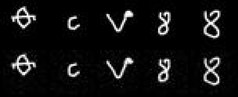
(a) Characters from the Omniglot evaluation set (above) and our model’s reconstructions (below)

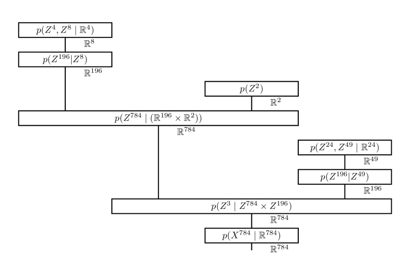
(b) An example string diagram drawn from the approximate posterior of the free category model.

Figure 1: Reconstructions (left) generated by inference in the diagrammatic generative model (right) on handwritten characters in the Omniglot evaluation set. The string diagram shows a model that generates a glimpse, decodes it into an image canvas via a variational ladder decoder, and then performs a simpler process to generate another glimpse and insert it into the canvas.

Table 1 compares the free category prior’s performance to other structured generative models (described in Appendix D). We report the estimated log model evidence (estimated as described in Appendix A). Our free category prior over deep generatives models achieves the best log-evidence per data dimension. Figure 1 shows samples from the trained model’s posterior distribution, including reconstruction of evaluation data (Figure 1(a)) and the morphism sampled for that data (Figure 1(b)).

5 Discussion

This paper described a probabilistic generative model over free categories. Section 3 gave a novel categorical description of distributions over morphisms, by enriching in QBS with joint distributions and push-forwards. It then showed how to sample morphisms from QBS-enriched free monoidal categories via a stochastic short-paths policy. Section 4 described the software implementation of the free category prior as Discopyro, showing that enriching in a Markov category can also be understood as randomly sampling the computational representations of morphisms in an SMC. It then showed that amortized variational inference in Discopyro achieved competitive log-likelihood in generative modeling of the Omniglot dataset. This section discusses potential future work.

Future improvements to the free category prior

The underlying quiver $Q$ could be expanded stochastically by randomly choosing and applying commuting diagrams (such as functors, universal constructions, etc.). In the infinite limit, such expansions would give a $Q$ encoding the “true” category given by the original graph and the commuting diagrams: a (nonparametric) probability model $\mathbb{P}(Q)$ over the category. This would provide a nonparametric category model as an alternative to nonparametric grammar (i.e. operad) models [36]. Stochastic memoization [59] would enable sampling from that model, with Russian Roulette methods [72] providing gradient estimates of Equation 12.

We defined the free category prior in terms of Estrada and Hatano’s [15] communicability quasimetric. Boyd et al. [5] recently published a proper metric on quivers and their Markov chains, which might provide a more interpretable foundation for our stochastic short-paths algorithm. Stochastically generalizing shortest-path algorithms may improve the tractability of credit-assignment in policy learning. We plan to explore a subgoal decomposition (e.g. such as Jurgenson’s[37]) of path-sampling.

Future improvements to the Discopyro implementation

Discopyro employs amortized variational inference to model the posterior distribution over morphisms. The inference functor mentioned in Section 4.2 was defined ad-hoc, meeting only the requirements for constructing faithful inverses [71] for string diagrams. We used QBS as a semantic category for our learned probabilistic programs, and it is not yet known whether QBS and QBS have all the conditionals necessary to encode Bayesian inversion as a dagger functor. Conjecture 1 hypothesizes explicitly that an inference construction similar to ours could approximate Bayesian inversions (in the sense of Cho and Jacobs [7]), rather than just a proposal.

Conjecture 1 (Approximate Bayesian inversions in $\mathbb{P}\>\mathbf{QBS}$).

Consider an inference functor $F^{\dagger}$ whose action on objects is identity, with action on morphisms similar to $F_{\_}q$ above. Such a functor is a dagger endofunctor $F^{\dagger}:\mathbb{P}\>\mathbf{QBS}\rightarrow\mathbb{P}\>\mathbf{QBS}$ sending objects to themselves and morphisms $f:\mathbf{QBS}(A,\mathbb{P}\>B)$ to (approximate) Bayesian inversions $f^{\dagger}:\mathbf{QBS}(B,\mathbb{P}\>A)$.

Conclusion

In our experiment the free category prior learned compositional structures from real data. Future applications could include learning program-like representations, a long-term goal for artificial intelligence [8, 40, 49], or “cognitive maps” for spatial navigation [44] in cognitive science [47].

Appendix A Estimation of log-likelihood by importance weighting

In approximate inference techniques based on importance weighting, we sample latent variables from a proposal density $q_{\_}\phi$ and then score them with an importance weight

$$w_{\_}{\theta,\phi} =\frac{p_{\_}\theta(x,z,f,\beta,W;\Phi,G)}{q_{\_}\phi(z,f,\beta,W\mid x)}$$ (10)

equal to the ratio of the proposal joint density over the latent variables and the generative joint density over all variables. This weighting adjusts for the bias of the proposal density, relative to the normalized generative joint density (that is, the Bayesian inverse or posterior distribution).

Lemma 5 (Importance weighting provides an estimator of the marginal density).

Given the generative and proposal joint distributions above, the expectation of the importance weights equals the marginal density of the observation

$$\mathbb{E}_{q_{\_}\phi(z,f,\beta,W\mid x;\Phi)}\left[w_{\_}{\theta,\phi}\right] =p_{\_}\theta(x;\Phi,G).$$ (11)

Finite samples approximating this expectation therefore provide Monte Carlo estimators of the analytically intractable marginal density:

$$p_{\_}\theta(x;\Phi,G) \approx\frac{1}{K}\sum_{\_}{k=1}^{K}w^{k}_{\_}{\theta,\phi}\text{ for }w^{k}_{\_}{\theta,\phi}\sim q_{\_}\phi(z,f,\beta,W\mid x;\Phi).$$

Proof.

We begin with the definition of the expected importance weight

$$\mathbb{E}_{q_{\_}\phi(z,f,\beta,W\mid x;\Phi)}\left[w_{\_}{\theta,\phi}\right] =\int\!{dz,f,\beta,W}\>q_{\_}\phi(z,f,\beta,W\mid x;\Phi)\>w_{\_}{\theta,\phi},$$

and expand it to include the density ratio

$$=\int\!{dz,f,\beta,W}\>q_{\_}\phi(z,f,\beta,W\mid x;\Phi)\>\left[\frac{p_{\_}\theta(x,z,f,\beta,W;\Phi,G)}{q_{\_}\phi(z,f,\beta,W\mid x)}\right],$$

$$=\int\!{dz,f,\beta,W}\>\>\frac{\cancel{q_{\_}\phi(z,f,\beta,W\mid x;\Phi)}p_{\_}\theta(x,z,f,\beta,W;\Phi,G)}{\cancel{q_{\_}\phi(z,f,\beta,W\mid x)}},$$

$$=\int\!{dz,f,\beta,W}\>p_{\_}\theta(x,z,f,\beta,W;\Phi,G)\>,$$

$$\mathbb{E}_{q_{\_}\phi(z,f,\beta,W\mid x;\Phi)}\left[w_{\_}{\theta,\phi}\right] =p_{\_}\theta(x;\Phi,G).$$

∎

This quantity can be estimated by Monte Carlo techniques, obtaining the estimator

$$Z_{\_}{\theta,\phi} \approx\frac{1}{K}\sum_{\_}{k=1}^{K}w_{\_}{\theta,\phi} \hat{Z}_{\_}{\theta,\phi} =\frac{1}{K}\sum_{\_}{k=1}^{K}w_{\_}{\theta,\phi}.$$

Resampling proportionally to these weights can then provide us with an unbiased sample from the true posterior distribution [9]. Storing the actual weights in log-space typically provides better numerical stability, when coupled to a specialized mean-exp implementation. In our case, PyTorch provides such an implementation.

Taking the logarithm of both sides of Equation 11 yields an expression known as the log-evidence for the model

$$\log\mathbb{E}_{q_{\_}\phi(z,f,\beta,W\mid x;\Phi)}\left[w_{\_}{\theta,\phi}\right] =\log p_{\_}\theta(x;\Phi,G),$$

and applying Jensen’s Inequality yields a variational lower bound to the log-evidence

$$\mathbb{E}_{q_{\_}\phi(z,f,\beta,W\mid x;\Phi)}\left[\log w_{\_}{\theta,\phi}\right] \leq\log p_{\_}\theta(x;\Phi,G).$$

We call the left-hand side of this inequality the Evidence Lower Bound (ELBO)

$$\mathcal{L}(\theta,\phi) =\mathbb{E}_{q_{\_}\phi(z,f,\beta,W\mid x;\Phi)}\left[\log w_{\_}{\theta,\phi}\right]\leq\log p_{\_}\theta(x;\Phi,G).$$ (12)

Appendix B will provide an alternate derivation for the ELBO, showing that maximizing the ELBO minimizes the (exclusive) Kullback Lieblier divergence from the proposal to the posterior distribution.

Appendix B Derivation of the ELBO objective

Any proposal like Equation 9 can help sample from the posterior distribution by importance weighting, but we can obtain progressively better approximations by minimizing the Kullback Liebler divergence (see [48] for details) from the proposal to the true posterior

$$\text{KL}(q_{\_}\phi(z,f,\beta,W\mid x)||p_{\_}\theta(z,f,\beta,W\mid x;\Phi,G)) =\mathbb{E}_{q_{\_}\phi(z,f,\beta,W\mid x)}\left[\log\frac{q_{\_}\phi(z,f,\beta,W\mid x)}{p_{\_}\theta(z,f,\beta,W\mid x;\Phi,G)}\right].$$

Equation 8 shows the true posterior to be

$$p_{\_}\theta(z,f,\beta,W\mid x;\Phi,G) =\frac{p_{\_}\theta(x,z,f,\beta,W;\Phi,G)}{p_{\_}\theta(x;\Phi,G)},$$

with the numerator being the joint distribution defined in Equation 7 above. Substituting the right-hand side of this equation into the definition of the divergence above

$$\text{KL}(q_{\_}\phi||p_{\_}\theta) =\mathbb{E}_{q_{\_}\phi(z,f,\beta,W\mid x)}\left[\log\frac{q_{\_}\phi(z,f,\beta,W\mid x)p_{\_}\theta(x;\Phi,G)}{p_{\_}\theta(x,z,f,\beta,W;\Phi,G)}\right],$$

$$=\mathbb{E}_{q_{\_}\phi(z,f,\beta,W\mid x)}\left[\log q_{\_}\phi(z,f,\beta,W\mid x)+\log p_{\_}\theta(x;\Phi,G)-\log p_{\_}\theta(x,z,f,\beta,W;\Phi,G)\right],$$

$$=\mathbb{E}_{q_{\_}\phi(z,f,\beta,W\mid x)}\left[\log q_{\_}\phi(z,f,\beta,W\mid x)-\log p_{\_}\theta(x,z,f,\beta,W;\Phi,G)\right]+\log p_{\_}\theta(x;\Phi,G),$$

$$=\mathbb{E}_{q_{\_}\phi(z,f,\beta,W\mid x)}\left[\log\frac{q_{\_}\phi(z,f,\beta,W\mid x)}{p_{\_}\theta(x,z,f,\beta,W;\Phi,G)}\right]+\log p_{\_}\theta(x;\Phi,G),$$

$$=\log p_{\_}\theta(x;\Phi,G)-\mathbb{E}_{q_{\_}\phi(z,f,\beta,W\mid x)}\left[\log\frac{p_{\_}\theta(x,z,f,\beta,W;\Phi,G)}{q_{\_}\phi(z,f,\beta,W\mid x)}\right]$$

shows that the divergence decomposes into two components: the log model evidence and the negative expected log importance weight. The sum of the expected log weight and the divergence is the log model evidence

$$\text{KL}(q_{\_}\phi||p_{\_}\theta)+\mathbb{E}_{q_{\_}\phi(z,f,\beta,W\mid x)}\left[\log\frac{p_{\_}\theta(x,z,f,\beta,W;\Phi,G)}{q_{\_}\phi(z,f,\beta,W\mid x)}\right] =\log p_{\_}\theta(x;\Phi,G),$$

so that the expected log weight itself

$$\mathbb{E}_{q_{\_}\phi(z,f,\beta,W\mid x)}\left[\log\frac{p_{\_}\theta(x,z,f,\beta,W;\Phi,G)}{q_{\_}\phi(z,f,\beta,W\mid x)}\right] =\log p_{\_}\theta(x;\Phi,G)-\text{KL}(q_{\_}\phi||p_{\_}\theta),$$

equals the log evidence minus the divergence. Since the divergence itself is always non-negative

$$\log p_{\_}\theta(x;\Phi,G)-\text{KL}(q_{\_}\phi||p_{\_}\theta) \leq\log p_{\_}\theta(x;\Phi,G)$$

$$\mathbb{E}_{q_{\_}\phi(z,f,\beta,W\mid x)}\left[\log\frac{p_{\_}\theta(x,z,f,\beta,W;\Phi,G)}{q_{\_}\phi(z,f,\beta,W\mid x)}\right] \leq\log p_{\_}\theta(x;\Phi,G),$$

the expected log-weight therefore provides a lower bound to the log-evidence. For this reason, we typically call it the Evidence Lower Bound (ELBO)

$$\mathcal{L}(\theta,\phi) =\mathbb{E}_{\_}{q_{\_}{\phi}}\left[\log\frac{p_{\_}\theta(x,z,f,\beta,W;\Phi,G)}{q_{\_}\phi(z,f,\beta,W\mid x)}\right],$$

and take it as an objective function to perform variational Bayesian inference [4]. The derivation above implies that maximizing $\mathcal{L}$ will minimize the divergence between the tractable proposal density and the intractable true posterior, with $\mathcal{L}$ equalling the true model-evidence only if the divergence reaches zero.

Appendix C Training and evaluation details

We parameterized the free category $\mathbf{Free}(Q)$ by generating input and output pairs from dimensionalities ranging from 4 to 196, picking powers of 2, and constructing the following build blocks for deep generative models:

1. Fully-connected VAE decoder networks. Decoders mapping down to $\mathbb{R}^{196}$ were considered to decode image glimpses, and therefore used transposed convolutional layers to produce their outputs;

2. Variational “Ladder” decoder and prior networks from Zhao [73]’s work on learning hierarchical features, with a noise dimension of 2; and

3. Spatial attention mechanisms from Rezende [57] which map $\mathbb{R}^{14\times 14}\rightarrow\mathbb{R}^{28\times 28}$, sampling a spatial transformation code $z\in\mathbb{R}^{3}$ from a learned Gaussian prior.

Attaching the likelihood to the generator morphism required sampling the free category prior via the two-part wiring diagram

$$f_{\_}{\theta} :\mathbf{QBS}(I,\mathbb{P}\>(\mathbb{R}^{28\times 28}\times\tau)) \ell_{\_}{\sigma} :\mathbf{QBS}(\mathbb{R}^{28\times 28},\mathbb{P}\>(\mathbb{R}^{28\times 28}\times(\mathtt{x}:\mathbb{R}^{28\times 28})))$$

$$f_{\_}{\theta}\fatsemi_{\_}{\mathbb{P}\>}\ell_{\_}{\sigma} :\mathbf{QBS}(I,\mathbb{P}\>(\mathbb{R}^{28\times 28}\times(\mathtt{x}:\mathbb{R}^{28\times 28}))).$$

$\mathcal{L}$ and its gradients were approximated by Monte Carlo sampling; Pyro [3]’s TraceGraphELBO class provided gradient estimators [46, 61]. We trained this model for 1200 epochs, with a learning rate $\eta=10^{-3}$. At test time we substitute a Bernoulli likelihood for the Gaussian, to “compare like to like” with other models in the literature.

Appendix D Dataset history and selection of competing models

Lake [39, 40] and colleagues proposed the Omniglot dataset to challenge the machine learning community to achieve human-like concept learning by learning a single generative model from very few examples; the Omniglot challenge requires that a model be usable for classification, latent feature recognition, concept generation from a type, and exemplar generation of a concept. The deep generative models research community has focused on producing models capable of few-shot reconstruction of unseen characters. Rezende [57] and Hewitt [34] fixed as constant the model architecture, attempting to account for the compositional structure in the data with static dimensionality. In contrast, He [31] and Feinman [16] jointly learned the model structure alongside inferring the posterior distribution over the latent variables and reconstructing the data.

References

- [1]
- [2] Alon B Baram, Timothy H Muller, James CR Whittington & Timothy EJ Behrens (2018): Intuitive planning: global navigation through cognitive maps based on grid-like codes. bioRxiv, p. 421461.
- [3] Eli Bingham, Jonathan P Chen, Martin Jankowiak, Fritz Obermeyer, Neeraj Pradhan, Theofanis Karaletsos, Rohit Singh, Paul Szerlip, Paul Horsfall & Noah D Goodman (2019): Pyro: Deep universal probabilistic programming. The Journal of Machine Learning Research 20(1), pp. 973–978.
- [4] David M. Blei, Alp Kucukelbir & Jon D. McAuliffe (2017): Variational Inference: A Review for Statisticians, 10.1080/01621459.2017.1285773. Available at http://arxiv.org/abs/1601.00670http://dx.doi.org/10.1080/01621459.2017.1285773.
- [5] Zachary M. Boyd, Nicolas Fraiman, Jeremy Marzuola, Peter J. Mucha, Braxton Osting & Jonathan Weare (2021): A Metric on Directed Graphs and Markov Chains Based on Hitting Probabilities. SIAM Journal on Mathematics of Data Science 3(2), pp. 467–493, 10.1137/20m1348315.
- [6] Richard A. Brualdi, Frank Harary & Zevi Miller (1980): Bigraphs versus digraphs via matrices. Journal of Graph Theory 4(1), pp. 51–73, https://doi.org/10.1002/jgt.3190040107. Available at https://onlinelibrary.wiley.com/doi/abs/10.1002/jgt.3190040107.
- [7] Kenta Cho & Bart Jacobs (2019): Disintegration and Bayesian inversion via string diagrams. Mathematical Structures in Computer Science 29(7), pp. 938–971, 10.1017/S0960129518000488.
- [8] François Chollet (2019): On the Measure of Intelligence, pp. 1–64. Available at http://arxiv.org/abs/1911.01547.
- [9] Nicolas Chopin & Omiros Papaspiliopoulos (2020): An Introduction to Sequential Monte Carlo. Springer, 10.1007/978-3-030-47845-2.
- [10] Stephen Clark, Bob Coecke & Mehrnoosh Sadrzadeh (2008): A compositional distributional model of meaning. In: Proceedings of the Second Quantum Interaction Symposium (QI-2008), Schuetze 1998, pp. 133–140.
- [11] G. S. H. Cruttwell, Bruno Gavranović, Neil Ghani, Paul Wilson & Fabio Zanasi (2021): Categorical Foundations of Gradient-Based Learning. In: Applied Category Theory Conference (ACT 2021). Available at http://arxiv.org/abs/2103.01931.
- [12] Jared Culbertson & Kirk Sturtz (2014): A categorical foundation for bayesian probability. Applied Categorical Structures 22(4), pp. 647–662, 10.1007/s10485-013-9324-9.
- [13] Fredrik Dahlqvist, Alexandra Silva, Vincent Danos & Ilias Garnier (2018): Borel Kernels and their Approximation, Categorically. Electronic Notes in Theoretical Computer Science 341, pp. 91–119, https://doi.org/10.1016/j.entcs.2018.11.006. Available at https://www.sciencedirect.com/science/article/pii/S1571066118300860. Proceedings of the Thirty-Fourth Conference on the Mathematical Foundations of Programming Semantics (MFPS XXXIV).
- [14] Conal Elliott (2017): Compiling to categories. Proceedings of the ACM on Programming Languages 1(ICFP), pp. 1–27, 10.1145/3110271.
- [15] Ernesto Estrada & Naomichi Hatano (2008): Communicability in complex networks. Physical Review E - Statistical, Nonlinear, and Soft Matter Physics 77(3), pp. 1–12, 10.1103/PhysRevE.77.036111.
- [16] Reuben Feinman & Brenden M. Lake (2021): Learning Task-General Representations with Generative Neuro-Symbolic Modeling. In: International Conference on Learning Representations. Available at http://arxiv.org/abs/2006.14448.
- [17] Giovanni de Felice, Alexis Toumi & Bob Coecke (2020): DisCoPy: Monoidal Categories in Python. In: Applied Category Theory Conference, pp. 1–20. Available at http://arxiv.org/abs/2005.02975.
- [18] Brendan Fong & Michael Johnson (2019): Lenses and learners. CEUR Workshop Proceedings 2355(Bx), pp. 16–29.
- [19] Brendan Fong, David Spivak & Remy Tuyeras (2019): Backprop as Functor: A compositional perspective on supervised learning. Proceedings - Symposium on Logic in Computer Science 2019-June, pp. 1–13, 10.1109/LICS.2019.8785665.
- [20] Brendan Fong & David I Spivak (2019): Seven Sketches in Compositionality: An Invitation to Applied Category Theory. Cambridge University Press. Available at http://arxiv.org/abs/1803.05316.
- [21] Steven M. Frankland & Joshua D. Greene (2020): Concepts and Compositionality: In Search of the Brain’s Language of Thought. Annual Review of Psychology 71(1), pp. 273–303, 10.1146/annurev-psych-122216-011829.
- [22] Tobias Fritz (2020): A synthetic approach to Markov kernels, conditional independence and theorems on sufficient statistics. Advances in Mathematics 370, p. 107239, 10.1016/j.aim.2020.107239. Available at https://doi.org/10.1016/j.aim.2020.107239.
- [23] Peter Gardenfors (2004): Conceptual spaces: The geometry of thought. MIT press.
- [24] Bruno Gavranovic (2019): Learning functors using gradient descent. In: Applied Category Theory Conference (ACT 2019), 323, Electronic Proceedings in Theoretical Computer Science, EPTCS, pp. 230–245, 10.4204/EPTCS.323.15.
- [25] Michele Giry (1982): A categorical approach to probability theory. In: Categorical aspects of topology and analysis, Springer, pp. 68–85.
- [26] Petr Viktorovich Golubtsov (1999): Axiomatic description of categories of information transformers. Problemy Peredachi Informatsii 35(3), pp. 80–98.
- [27] Erin Grant, Joshua C. Peterson & Tom Griffiths (2019): Learning deep taxonomic priors for concept learning from few positive examples. In: The Annual Meeting of the Cognitive Science Society, pp. 1865–1870. Available at https://www.semanticscholar.org/paper/Learning-deep-taxonomic-priors-for-concept-learning-Grant-Peterson/8eef236bca7ed58f8fa96786925c0e1da4a124eb.
- [28] Edward Grefenstette & Mehrnoosh Sadrzadeh (2011): Experimental support for a categorical compositional distributional model of meaning. In: EMNLP 2011 - Conference on Empirical Methods in Natural Language Processing, Proceedings of the Conference, pp. 1394–1404.
- [29] Micah Halter, Evan Patterson, Andrew Baas & James Fairbanks (2020): Compositional Scientific Computing with Catlab and SemanticModels, pp. 1–3. Available at http://arxiv.org/abs/2005.04831.
- [30] Uri Hasson, Samuel A. Nastase & Ariel Goldstein (2020): Direct Fit to Nature: An Evolutionary Perspective on Biological and Artificial Neural Networks. Neuron 105(3), pp. 416–434, 10.1016/j.neuron.2019.12.002. Available at https://doi.org/10.1016/j.neuron.2019.12.002.
- [31] Jiawei He, Yu Gong, Greg Mori, Joseph Marino & Andreas M. Lehrmann (2019): Variational autoencoders with jointly optimized latent dependency structure. In: 7th International Conference on Learning Representations, ICLR 2019, pp. 1–16.
- [32] C. Hermida, M. Makkai & J. Power (1998): Higher dimensional multigraphs. In: Proceedings. Thirteenth Annual IEEE Symposium on Logic in Computer Science (Cat. No.98CB36226), pp. 199–206, 10.1109/LICS.1998.705656.
- [33] Chris Heunen, Ohad Kammar, Sam Staton & Hongseok Yang (2017): A convenient category for higher-order probability theory. In: Proceedings - Symposium on Logic in Computer Science, 10.1109/LICS.2017.8005137.
- [34] Luke B. Hewitt, Maxwell I. Nye, Andreea Gane, Tommi Jaakkola & Joshua B. Tenenbaum (2018): The Variational Homoencoder: Learning to learn high capacity generative models from few examples. 34th Conference on Uncertainty in Artificial Intelligence 2018, UAI 2018 2, pp. 988–997.
- [35] Mark K Ho & Tom Griffiths (2018): Human Priors in Hierarchical Program Induction. In: Cognitive Computational Neuroscience, 1. Available at http://lightbot.com.
- [36] Mark Johnson, Thomas Griffiths & Sharon Goldwater (2006): Adaptor grammars: A framework for specifying compositional nonparametric Bayesian models. Advances in neural information processing systems 19.
- [37] Tom Jurgenson, Or Avner, Edward Groshev & Aviv Tamar (2020): Sub-goal trees – A framework for goal-based reinforcement learning. In: 37th International Conference on Machine Learning, ICML 2020, pp. 5020–5030.
- [38] Brenden M. Lake & Steven T. Piantadosi (2019): People infer recursive visual concepts from just a few examples. Computational Brain & Behavior. Available at http://arxiv.org/abs/1904.08034.
- [39] Brenden M. Lake, Ruslan Salakhutdinov & Joshua B. Tenenbaum (2015): Human-level concept learning through probabilistic program induction. Science 350(6266), pp. 1332–1338, 10.1126/science.aab3050. Available at http://science.sciencemag.org/content/350/6266/1332https://www.sciencemag.org/content/350/6266/1332.full.pdf.
- [40] Brenden M. Lake, Ruslan Salakhutdinov & Joshua B. Tenenbaum (2019): The Omniglot challenge: a 3-year progress report. Current Opinion in Behavioral Sciences 29, pp. 97–104, 10.1016/j.cobeha.2019.04.007. Available at https://doi.org/10.1016/j.cobeha.2019.04.007.
- [41] Guy Latouche & Vaidyanathan Ramaswami (1999): Introduction to Matrix Analytic Methods in Stochastic Modeling. Society for Industrial and Applied Mathematics, Philadelphia, PA.
- [42] Alexander K. Lew, Marco F. Cusumano-Towner, Benjamin Sherman, Michael Carbin & Vikash K. Mansinghka (2020): Trace Types and Denotational Semantics for Sound Programmable Inference in Probabilistic Languages. In: ACM Principles of Programming Languages, 4, pp. 1–31, 10.1145/3371087.
- [43] Gary F Marcus (2018): The algebraic mind: Integrating connectionism and cognitive science. MIT press.
- [44] Jade Master (2021): The Open Algebraic Path Problem. In Fabio Gadducci & Alexandra Silva, editors: 9th Conference on Algebra and Coalgebra in Computer Science (CALCO 2021), Leibniz International Proceedings in Informatics (LIPIcs) 211, Schloss Dagstuhl – Leibniz-Zentrum für Informatik, Dagstuhl, Germany, pp. 20:1–20:20, 10.4230/LIPIcs.CALCO.2021.20. Available at https://drops.dagstuhl.de/opus/volltexte/2021/15375.
- [45] Jan-Willem van de Meent, Brooks Paige, Hongseok Yang & Frank Wood (2018): An introduction to probabilistic programming. arXiv preprint arXiv:1809.10756.
- [46] Andriy Mnih & Karol Gregor (2014): Neural variational inference and learning in belief networks. In: 31st International Conference on Machine Learning, ICML 2014, 5, pp. 3800–3809.
- [47] Ida Momennejad (2020): Learning Structures: Predictive Representations, Replay, and Generalization. Current Opinion in Behavioral Sciences 32, pp. 155–166, 10.1016/j.cobeha.2020.02.017. Available at https://doi.org/10.1016/j.cobeha.2020.02.017.
- [48] P K Murphy (2012): Machine Learning: A Probabilistic Perspective. 10.1007/SpringerReference35834.
- [49] Weili Nie, Zhiding Yu, Lei Mao, Ankit B. Patel, Yuke Zhu & Animashree Anandkumar (2020): Bongard-LOGO: A New Benchmark for Human-Level Concept Learning and Reasoning. In: Advances in Neural Information Processing Systems, NeurIPS. Available at http://arxiv.org/abs/2010.00763.
- [50] Maxwell I. Nye, Armando Solar-Lezama, Joshua B. Tenenbaum & Brenden M. Lake (2020): Learning compositional rules via neural program synthesis. Advances in Neural Information Processing Systems 2020-December(NeurIPS), pp. 1–11.
- [51] Matthew C. Overlan, Robert A. Jacobs & Steven T. Piantadosi (2017): Learning abstract visual concepts via probabilistic program induction in a Language of Thought. Cognition 168, pp. 320–334, 10.1016/j.cognition.2017.07.005. Available at http://dx.doi.org/10.1016/j.cognition.2017.07.005.
- [52] Emilio Parisotto, Abdel-rahman Mohamed, Rishabh Singh, Lihong Li, Dengyong Zhou & Pushmeet Kohli (2017): Neuro-Symbolic Program Synthesis. In: International Conference on Learning Representations, pp. 1–14. Available at http://arxiv.org/abs/1611.01855.
- [53] Evan Patterson, Owen Lynch & James Fairbanks (2021): Categorical Data Structures for Technical Computing, pp. 1–28. Available at https://arxiv.org/abs/2106.04703.
- [54] Evan Patterson, David I. Spivak & Dmitry Vagner (2021): Wiring diagrams as normal forms for computing in symmetric monoidal categories. Electronic Proceedings in Theoretical Computer Science, EPTCS 333, pp. 49–64, 10.4204/EPTCS.333.4.
- [55] Steven Phillips & William H. Wilson (2010): Categorial Compositionality: A Category Theory Explanation for the Systematicity of Human Cognition. PLOS Computational Biology 6(7), pp. 1–14, 10.1371/journal.pcbi.1000858. Available at https://doi.org/10.1371/journal.pcbi.1000858.
- [56] Steven T. Piantadosi, Joshua B. Tenenbaum & Noah D. Goodman (2016): The logical primitives of thought: Empirical foundations for compositional cognitive models. Psychological Review 123(4), pp. 392–424, 10.1037/a0039980.
- [57] Danilo Jimenez Rezende, Shakir Mohamed, Ivo Danihelka, Karol Gregor & Daan Wierstra (2016): One-Shot Generalization in Deep Generative Models. In: International Conference on Machine Learning, 48.
- [58] Sergio Romano, Alejo Salles, Marie Amalric, Stanislas Dehaene, Mariano Sigman & Santiago Figueira (2018): Bayesian validation of grammar productions for the language of thought. PLoS ONE 13(7), pp. 1–20, 10.1371/journal.pone.0200420.
- [59] Daniel M Roy, VK Mansinghka, ND Goodman & JB Tenenbaum (2008): A stochastic programming perspective on nonparametric Bayes. In: Nonparametric Bayesian Workshop, Int. Conf. on Machine Learning, 22, p. 26.
- [60] Dylan Rupel & David I. Spivak (2013): The operad of temporal wiring diagrams: formalizing a graphical language for discrete-time processes, pp. 1–37. Available at http://arxiv.org/abs/1307.6894.
- [61] John Schulman, Nicolas Heess, Theophane Weber & Pieter Abbeel (2015): Gradient estimation using stochastic computation graphs. In: Advances in Neural Information Processing Systems, 2015-Janua, pp. 3528–3536.
- [62] Adam Ścibior, Ohad Kammar, Matthijs Vákár, Sam Staton, Hongseok Yang, Yufei Cai, Klaus Ostermann, Sean K. Moss, Chris Heunen & Zoubin Ghahramani (2018): Denotational validation of higher-order Bayesian inference. In: Principles of Programming Languages, 2, 10.1145/3158148.
- [63] Dan Shiebler, Bruno Gavranović & Paul Wilson (2021): Category Theory in Machine Learning. In: Applied Category Theory Conference. Available at http://arxiv.org/abs/2106.07032.
- [64] R J Solomonoff (1964): A formal theory of inductive inference. Part I. Information and Control 7(1), pp. 1–22, https://doi.org/10.1016/S0019-9958(64)90223-2. Available at http://www.sciencedirect.com/science/article/pii/S0019995864902232.
- [65] Morten Heine Sørensen & Pawel Urzyczyn (2006): Lectures on the Curry-Howard isomorphism. Elsevier.
- [66] David I Spivak (2013): The operad of wiring diagrams: formalizing a graphical language for databases, recursion, and plug-and-play circuits. arXiv preprint arXiv:1305.0297.
- [67] Andreas Stuhlmüller, Jacob Taylor & Noah Goodman (2013): Learning Stochastic Inverses. In C. J. C. Burges, L. Bottou, M. Welling, Z. Ghahramani & K. Q. Weinberger, editors: Advances in Neural Information Processing Systems, 26, Curran Associates, Inc. Available at https://proceedings.neurips.cc/paper/2013/file/7f53f8c6c730af6aeb52e66eb74d8507-Paper.pdf.
- [68] Lazar Valkov, Dipak Chaudhari, Charles Sutton, Akash Srivastava & Swarat Chaudhuri (2018): Houdini: Lifelong learning as program synthesis. In: Advances in Neural Information Processing Systems, 2018-Decem, pp. 8687–8698.
- [69] Paul M.B. Vitányi & Ming Li (2000): Minimum description length induction, Bayesianism, and Kolmogorov complexity. IEEE Transactions on Information Theory 46(2), pp. 446–464, 10.1109/18.825807.
- [70] R. F.C. Walters (1989): The free category with products on a multigraph. Journal of Pure and Applied Algebra 62(2), pp. 205–210, 10.1016/0022-4049(89)90152-7.
- [71] Stefan Webb, Adam Goliński, Robert Zinkov, N. Siddharth, Tom Rainforth, Yee Whye Teh & Frank Wood (2018): Faithful Inversion of Generative Models for Effective Amortized Inference. In: Proceedings of the 32nd International Conference on Neural Information Processing Systems, NIPS’18, Curran Associates Inc., Red Hook, NY, USA, p. 3074–3084.
- [72] Kai Xu, Akash Srivastava & Charles Sutton (2019): Variational Russian Roulette for Deep Bayesian Nonparametrics. In Kamalika Chaudhuri & Ruslan Salakhutdinov, editors: Proceedings of the 36th International Conference on Machine Learning, Proceedings of Machine Learning Research 97, PMLR, pp. 6963–6972. Available at https://proceedings.mlr.press/v97/xu19e.html.
- [73] Shengjia Zhao, Jiaming Song & Stefano Ermon (2017): Learning Hierarchical Features from Generative Models. In: International Conference on Machine Learning. Available at http://arxiv.org/abs/1702.08396.
- [74] Yanli Zhou & Brenden M. Lake (2021): Flexible Compositional Learning of Structured Visual Concepts. In: Proceedings of the 43rd Annual Conference of the Cognitive Science Society. Available at http://arxiv.org/abs/2105.09848.