Repeated Averages on Graphs

Abstract

Sourav Chatterjee, Persi Diaconis, Allan Sly and Lingfu Zhang ([Chatterjee et al., 2021]), prompted by a question of Ramis Movassagh, renewed the study of a process proposed in the early 1980s by Jean Bourgain. A state vector $v\in\mathbb{R}^{n}$, labeled with the vertices of a connected graph, $G$, changes in discrete time steps following the simple rule that at each step a random edge $(i,j)$ is picked and $v_{i}$ and $v_{j}$ are both replaced by their average $(v_{i}+v_{j})/2$. It is easy to see that the value associated with each vertex converges to $1/n$. The question was how quickly will $v$ be $\epsilon$-close to uniform in the $L^{1}$ norm in the case of the complete graph, $K_{n}$, when $v$ is initialized as a standard basis vector that takes the value 1 on one coordinate, and zeros everywhere else. They have established a sharp cutoff of $\frac{1}{2\log 2}n\log n+O(n\sqrt{\log n})$. Our main result is to prove, that $\frac{(1-\epsilon)}{2\log 2}n\log n-O(n)$ is a general lower bound for all connected graphs on $n$ nodes. We also get sharp magnitude of $t_{\epsilon,1}$ for several important families of graphs, including star, expander, dumbbell, and cycle. In order to establish our results we make several observations about the process, such as the worst case initialization is always a standard basis vector. Our results add to the body of work of Aldous [1989], Aldous and Lanoue [2012], Quattropani and Sau [2021], Cao [2021], Olshevsky and Tsitsiklis [2009], and others. The renewed interest is due to an analogy to a question related to the Google’s supremacy circuit. For the proof of our main theorem we employ a concept that we call augmented entropy function which may find independent interest in the computer science and probability theory communities.

1 Introduction

1.1 The Averaging Process

Let $G=\left(V(G),E(G)\right)$ be an undirected, connected finite graph. The averaging process on $G$ proceeds in discrete time steps, $t=0,1,\ldots$. At $t=0$ there is a real number associated with each node of the graph, defining the initial vector, $v(0)$. In each step, $t=1,2,\ldots$, we pick an edge randomly and uniformly from $E$ and replace the values associated with both of its end points of this edge by their average. Let $(v_{1},\dots,v_{n})^{T}$ denote the state vector at a given time. If in the next step an edge $(i,j)\in E$ is picked, the new state vector becomes

$$\left(v_{1},\;\dots,\;v_{i-1},\;\frac{v_{i}+v_{j}}{2},v_{i+1},\;\dots,v_{j-1},\;\frac{v_{i}+v_{j}}{2},\;v_{j+1},\;\dots,\;v_{n}\right)^{T}.$$

Let $v(t)=(v_{1}(t),\dots,v_{n}(t))^{T}$ be the value of $v$ in the $t^{\rm th}$ step ($t=0,1,2,\ldots$). The expression $\frac{1}{n}\sum_{i=1}^{n}v_{i}(t)$ remains invariant in every branch of the process. Let

$${\bar{v}}\equiv(a,\dots,a)^{T},\;\;\;\;\;{\rm where}\;\;\;\;\;a\equiv\frac{1}{n}\sum_{i=1}^{n}v_{i}(0)$$

An easy argument shows that for large enough $t$ the state vector $v(t)$ will be very likely in the proximity of ${\bar{v}}$. Most results, including ours, investigate the speed of convergence to ${\bar{v}}$. This speed depends on ($i$) the graph $G$, ($ii$) the initial vector $v(0)$, and ($iii$) the notion of convergence. The convergence in the $L^{2}$ norm is easy to analyse, but it is less interesting than the convergence in the $L^{1}$ norm, which is the main subject of our study. We will also study $2\rightarrow 1$ convergence defined below. To capture the quantities we are interested in, we have developed the following general definition:

Definition 1 ($\epsilon$-mixing time for $L^{q}$ metric under the unit $L^{p}$ sphere initialization).

$$t_{\epsilon,\,p\rightarrow q}(G)\equiv\min\left\{t\in\mathbb{N}\;\middle|\;\scaleto{\forall\mathstrut}{15pt}\;v(0)\;{\rm with}\;\lVert v(0)\rVert_{p}=1:\;\sqrt[\scaleto{q\mathstrut}{8pt}]{\mathbb{E}\left[\lVert v(t)-\bar{v}\rVert_{q}^{q}\right]}\leq\epsilon\right\},$$

where $\lVert w\rVert_{q}$ is $\sqrt[\scaleto{q\mathstrut}{8pt}]{\sum w_{i}^{q}}$, the $L^{q}$ norm.

We may omit $G$ in the argument when clear from the context. Further, when $p=q$, we simply say “$L^{p}$ convergence,” “$L^{p}$ mixing time” and we write “$t_{\epsilon,p}(G)$.” Notice that $\lVert v(t)-\bar{v}\rVert_{q}^{q}$ is a random variable, and Definition 1 focuses on its expectation.

Let $A(G)$ be the adjacency matrix of $G$ and $D(G)$ be the diagonal matrix formed from the vertex degrees of $G$. The spectrum of the graph Laplacian, $D(G)-A(G)$, is a well-known aid in analysing random walks on $G$. All eigenvalues of $L(G)$ are non-negative, the smallest of which is zero, while the second smallest, $\lambda_{2}(G)$ is a controlling parameter that roughly tells how quickly the random walk on $G$ mixes. In our case the following parameter will be central:

Definition 2.

For a connected, undirected graph $G=(V,E)$, we define

$$\gamma(G)=\frac{|E(G)|}{\lambda_{2}(G)}.$$

Since $\lambda_{2}(G)>0$ for every connected graph Fiedler [1973], we have $\gamma(G)<\infty$.

1.2 Main results

Throughout we will use the notation $f(x,\epsilon)=\Theta_{\epsilon}(g(x,\epsilon))$ when constants $c_{\epsilon},C_{\epsilon}$ exist that depend only on $\epsilon$ exist such that $c_{\epsilon}g(x,\epsilon)\leq f(x,\epsilon)\leq C_{\epsilon}g(x,\epsilon)$. We may omit the $\epsilon$ subscipt when $c_{\epsilon}$ and $C_{\epsilon}$ need not depend on $\epsilon$.

We compute or estimate the mixing times $t_{\epsilon,1}$ and $t_{\epsilon,2\rightarrow 1}$ (see Definition 1). The $L^{1}$ convergence, $t_{\epsilon,1}$, is the focus of most other works.

For all norms the quantity $\gamma(G)$ defined in Definition 2 determines convergence up-to a logarithmic factor, and the question is when this factor or some part of it is present. It has been observed earlier by several authors, that $t_{\epsilon,2}(G)=\Theta(\gamma(G))$ for every fixed $0<\epsilon<1$, and the constant factor is not large (about $2$). We show that the $t_{\epsilon,2\rightarrow 1}$ mixing time is also $\Theta(\gamma(G))$ when the graph Laplacian $L(G)$ admits a delocalized Fiedler vector – the eigenvector the corresponds to the second smallest eigenvalue (Theorem 8). For the $L^{1}$ mixing time we prove:

Theorem 1.

For any connected graph $G$ with $n$ nodes, the $\epsilon$-mixing time satisfies

$$t_{\epsilon,1}(G)\geq\frac{(1-\epsilon)}{2\log 2}n\log n-O(n)$$

Our bound does not only beat the standard argument’s general $\Omega(n)$ lower bound, but matches up-to a factor of $1-\epsilon$ with the sharp threshold of Sourav Chatterjee, Persi Diaconis, Allan Sly and Lingfu Zhang ([Chatterjee et al., 2021]) for the complete graph. Thus our result essentially shows that the complete graph asymptotically mixes fastest in the $L^{1}$ metric.

We conjecture, that $t_{\epsilon,1}(G)=\Theta_{\epsilon}(\max\{\gamma(G),n\log n\})$ (Conjecture 1). Towards the conjecture we derive several useful results on general graphs. In particular, the following result gives the slowest initialization under the $L^{1}$-metric, which can be of use in future research.

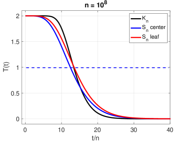
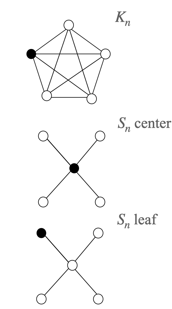
Figure 1: Expected $L^{1}$ convergence of the Averaging Process for the 100,000,000 node $K_{n}$ and for the star graph, $S_{n}$, of the same size with two different starting states (averaged over $20$ runs in each of the three cases; $T(t)$ estimates the expectation $\mathbb{E}[||v(t)-\frac{1}{n}{\bf 1}||_{1}]$ for the respective graphs). Interestingly, the star graph may slightly beat $K_{n}$, when the initial vector is $1$ at the center, although our theorem implies, that even when this is the case, it must be a lower order advantage.

Theorem 2 (Slowest initialization is at the corner).

Let $G$ be a graph with $n$ nodes. For every fixed $t$, the slowest initialization:

$$\operatorname*{arg\,max}_{v(0):\lVert v(0)\rVert_{1}=1}\mathbb{E}\lVert v(t)-\bar{v}\rVert_{1}=e_{i}$$

for some $i$, where

$$e_{i}=(0,\cdots,0,1,0,\cdots,0)$$

only has its $i$-th coordinate equals $1$.

Consequently, we get sharp magnitude of $t_{\epsilon,1}$ for several important families of graphs, with results summarized below. All our existing results support Conjecture 1. Our result on cycles resolve a conjecture in Spiro [2021], independently from Quattropani and Sau [2021], and with different techniques.

Graph	Bounded deg. expander	Star	Dumbbell	Cycle
$\boldsymbol{t_{\epsilon,1}}$	$\Theta_{\epsilon}(n\log n)$ (Prop 5)	$\Theta_{\epsilon}(n\log n)$ (Cor 4)	$\Theta_{\epsilon}(n^{3})$ (Thm 6)	$\Theta_{\epsilon}(n^{3})$ (Thm 7)

Table 1: The $L^{1}$ mixing time for selected graphs (each with $n$ nodes).

This paper provides several new techniques for the study of the averaging process. For example, the universal $\Omega(n\log n)$ lower bound relies on a novel augmented entropy function (see Definition 6). The mixing time for several families of graphs is based on ‘flow’, ‘comparison’ and ‘splitting’ techniques that are introduced and developed in this paper. These techniques may be of independent interest, and a utility for further investigations.

1.3 Open problems

Regarding the $L^{1}$ mixing time, evidences point towards

Conjecture 1.

Let $G$ be any connected graph with $n$ nodes,

$$\qquad t_{\epsilon,1}(G)=\Theta_{\epsilon}(\max\{\gamma(G),n\log n\})$$

We also think that in the case of $t_{\epsilon,2\rightarrow 1}$, which is immediate between $t_{\epsilon,2}(G)$ and $t_{\epsilon,1}(G)$, the $\log n$ factor is always present:

Conjecture 2.

Let $G$ be any connected graph with $n$ nodes,

$$\qquad t_{\epsilon,2\rightarrow 1}=\Theta_{\epsilon}(\gamma(G)\log n)$$

It is natural to inquire the cut-off phenomenon for different families of graphs. In [Chatterjee et al., 2021], the authors prove a cut-off phenomenon for the complete graph. It is also proved in Quattropani and Sau [2021] that certain families of graphs do not exhibit cut-offs. Are there other graphs for which one can prove or disprove a cut-off phenomenon, for instance for star graphs?

1.4 Organization

The result of this paper is organized as follows. After motivation and a discussion of previous work in Section 2, we state and prove the convergence speed of the averaging process under $L^{2}$, $L^{1}$, and $L^{2\rightarrow 1}$ metrics in Section 3.1, 3.2 and 3.3, respectively. Some numerical explorations are provided in Section 4. We introduce a related random process and prove the extremity of the complete graph in Section 5. Useful properties of the averaging process, and some technical proofs are provided in Section 6.

2 Motivation and previous work

Repeated averages (an alternative term for the averaging process in some literature) is a simple model for reaching equilibrium in statistical physics. Suppose each vertex value $v_{i}$ is a local temperature. We can envision an interaction that brings this system to thermal equilibrium. In much of statistical physics the equilibrium is reached via intermediate partial equilibria, where local patches reach an equilibrium and then each patch equilibrates with neighboring patches till full equilibrium is reached [Landau and Lifshitz, 2013, Vol. 5, Section 4]. Therefore, it is more realistic to consider the averaging process with respect to a locality constraint of the underlying system such as a graph structure or a lattice.

Another motivation comes from a toy model of quantum supremacy circuits, in which each gate enacts a unitary matrix drawn independently from the Haar measure. This random circuit family itself is an abstraction of Google’s Sycamore circuit Boixo et al. [2018], Arute et al. [2019]. Despite intensive research it remains open to prove that upon measurement and for a randomly selected member of the above family (with appropriate depth and connectivity parameters) the output distribution of the $2^{n}$ possible output strings approaches what is known as the Porter-Thomas distribution.

The effect of a Haar-local unitary is that regardless of the input to each gate, the output probability is the same for all possible outcomes. A key question is: how many such local gates should be applied for the overall output to reach the Porter-Thomas distribution? This crucially depends on the so-called architecture of the quantum circuit, which is the underlying graph of connectivity that dictates the position of the gates in the course of the computation. Therefore, both the power of a quantum circuit and its convergence to the desired output are dependent on the graph that defines the circuit architecture. The averaging process is a classical abstraction of these random quantum circuits.

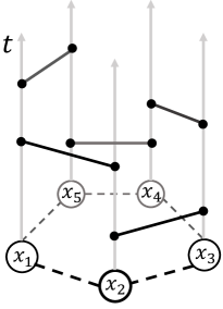
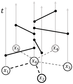
Figure 2: Schematics of the classical randomized swap gate circuit. Left: Circuit has a cycle architecture. Right: Circuit has a star architecture.

Our toy model is even simpler. It is a family of classical randomized circuits with 2-bit randomized swap gates. Each gate independently flips an unbiased coin. If Heads, the gate does not change the two bits involved. If Tails, the two bits are swapped. Given a graph, $G$, and a depth parameter $m$, we can define a randomized circuit family ${\cal F}(G,m)$ as follows. The nodes of $G$ correspond to input bits. Edges of $G$ represent bit-pairs where randomized swap gates can be placed. Example circuits for the star and circle graphs are shown in Figure 2. In the family ${\cal F}(G,m)$ each member of the family performs a sequence of $m$ gates $g_{1},\ldots,g_{m}$, where $g_{i}$ is randomly selected from $E(G)$. Assume now that we start with a distribution $p_{1},\ldots,p_{n}$ on inputs $e_{1},\ldots,e_{n}$, where $e_{i}=(0\cdots 0,\underbrace{1}_{i},0\cdots 0)^{T}$. The output is also a distribution on strings of Hamming weight one, since the application of each gate leaves the Hamming weight unchanged. For a random member of the family ${\cal F}(G,m)$ the output-distribution vector, $q$, distributes in the same way as $v(m)$ of the averaging process (in both cases we talk about distribution on vectors), where $v(0)=(p_{1},\ldots,p_{n})^{T}$, and the underlying graph is $G$. Further motivation for the averaging process can be found in Section 1.1 of Chatterjee et al. [2021].

The averaging process we study has been the subject of various works. Most notably, Aldous and Lanoue [2012] give a survey entitled “Lectures on the averaging process,” where the problem is expressed in the language of continuous-time Markov chains. Convergence in $L^{2}$ and entropy are investigated in connection with the spectral gap. Spiro [2021] derives upper bounds for the $L^{2}$ convergence of the averaging process on hyper-graphs.

[Chatterjee et al., 2021] focused on the $L^{1}$ convergence in the special case of the complete graph. They succeeded in showing a sharp cutoff phenomenon answering a conjecture of Jean Bourgain and a question of Ramis Movassagh. They proved that the $L^{1}$ convergence happens in time ${1\over 2\log 2}n\log n$ and the cutoff window is of magnitude $n\sqrt{\log n}$.

Quattropani and Sau [2021] considers a dual problem to averaging and characterizes the $L^{1}$ mixing time. They analyze the cutoff phenomena with respect to the number of random walkers on the graph.

Lastly, Cao [2021] derives the convergence to the uniform state of the averaging process on the complete graph from the exponential decay of the “Gini index” to zero in the continuum hydrodynamic limit.

There are a number of other works that investigate processes closely related to the averaging process. For example, Olshevsky and Tsitsiklis [2009] consider the averaging and consensus finding problems, where they mainly focus on the expected state vector under the averaging process. Shah’s 127 pages manuscript Shah [2009] on Gossip Algorithms derives mixing times and conductance for various graphs. Häggström [2012] considers the Deffuant model in the context of social interactions, where the graph has vertices on the integers with nearest-neighbor interactions. The underlying process averages the randomly chosen adjacent nodes with the possibility of “censorship”. They characterize the compatibility of social interactions as a function of the parameters of the underlying process. [Jain et al., 2020] consider the Kac walk with the aim of finding efficient algorithms for dimension reduction. For a set of special parameters their construction resembles the averaging process.

3 Convergence for the averaging process

This section includes our theoretical results. Some detailed proofs are deferred to the Appendix. Preliminary useful properties that we will directly use here are also proved in the Appendix (Section 6.1).

3.1 $L^{2}$ convergence

The $L^{2}$ convergence of the process is standard to analyze. We have that for every connected graph $G$ with $n$ nodes,

$$(2\gamma(G)-1)\log(\epsilon^{-1})\leq t_{\epsilon,2}(G)\;\leq\;4\gamma(G)\log(\epsilon^{-1})$$

whereas,

$$(2\gamma(G)-1)\log(\epsilon^{-1})\;\leq\;\{t_{\epsilon,1}(G),\;t_{\epsilon,2\rightarrow 1}(G)\}\;\leq\;4\gamma(G)\log(\sqrt{n}\epsilon^{-1})$$ (1)

We notice that replacing $(v_{i},v_{j})$ by $\left(\frac{v_{i}+v_{j}}{2},\frac{v_{i}+v_{j}}{2}\right)$ decreases $\mathbb{E}\left[\left\|v(t)-\bar{v}\right\|_{2}^{2}\right]$ exactly by $(v_{i}-v_{j})^{2}/2$. Based on this observation we have the following theorem. The proof details can be found in Section 6.2.1. The upper bound for Theorem 3 appears in Aldous and Lanoue [2012].

Theorem 3.

Let $v(0)\in\mathbb{R}^{n}$ be an arbitrary initial vector. Then the expected $L^{2}$ distance satisfies

$$\sqrt{\mathbb{E}\left[\left\|v(t)-\bar{v}\right\|_{2}^{2}\right]}\leq\left(1-\frac{1}{2\gamma(G)}\right)^{t/2}\left\|\bar{v}-v(0)\right\|_{2}\quad.$$ (2)

Furthermore, the slowest convergence speed is at least $\left(1-1/(2\gamma(G))\right)^{t}:$

$$\sup_{\left\|v(0)\right\|_{2}=1}\sqrt{\mathbb{E}\left[\left\|v(t)-\bar{v}\right\|_{2}^{2}\right]}\geq\left(1-\frac{1}{2\gamma(G)}\right)^{t}\quad.$$ (3)

We are in the position to bound the mixing time, which is the time it takes for the distribution of the state vector to be $\epsilon$-close to the uniform vector with respect to the norm of interest. The next corollary shows the $\epsilon$-mixing time under the $L^{2}$ metric is $\Theta(\gamma(G)\log(\epsilon^{-1}))$. The proof details can be found in Section 6.2.2.

Corollary 1.

($L^{2}$ mixing time)

$$(2\gamma(G)-1)\log\epsilon^{-1}\leq t_{\epsilon,2}\leq 4\gamma(G)\log\epsilon^{-1}\quad$$ (4)

With Corollary 1 in hand, we are able to analyze the $L^{2}$ mixing time for several natural families of graphs. Our results are summarized in Table 2 below, see Section 6.2.3 for proof details.

Graph	Complete graph $K_{n}$	Binary tree $B_{n}$	Star $S_{n-1}$	Cycle $C_{n}$
$\boldsymbol{t_{\epsilon,2}}$	$\Theta(n)\log\epsilon^{-1}$	$\Theta(n^{2})\log\epsilon^{-1}$	$\Theta(n)\log\epsilon^{-1}$	$\Theta(n^{3})\log\epsilon^{-1}$

Table 2: The $L^{2}$ mixing time for selected graphs

3.2 $L^{1}$ convergence

Although the $L^{2}$ distance is often regarded the natural metric for its mathematical convenience, two special reasons motivate the study of $L^{1}$ distance. First, the $L^{1}$ metric has a natural interpretation in probability theory. Any discrete probability measure is a unit vector under the $L^{1}$ metric, with non-negative coordinates. If the starting vector, $v(0)$, is a probability distribution, it remains so during the entire process. We then look at how quickly this distribution tends to uniform measured in total variation distance. Second, it is proved in [Chatterjee et al., 2021] that for the averaging process the $L^{1}$ convergence behaves differently from the $L^{2}$ convergence for the complete graph. They show that it takes $\Theta(n)$ steps to converge in $L^{2}$ metric, but $\frac{1}{2}(n\log_{2}n+c\,n\sqrt{\log_{2}n)}$ steps to converge in $L^{1}$ metric.

In this section we turn to study of the $\epsilon$-mixing time, $t_{\epsilon,1}$.

From the standard $L^{2}$ techniques we have the following upper and lower bounds, see Section 6.3.1 for proof details.

Theorem 4 (General bounds for $t_{\epsilon,1}$).

$$\left(2\gamma(G)-1\right)\log\epsilon^{-1}\;\leq\;t_{\epsilon,1}\;\leq\;4\gamma(G)(\log\sqrt{n}+\log\epsilon^{-1})$$ (5)

Equation (5) gives the $L^{1}$ mixing time up to a $\log n$ factor.

In this section we develop techniques to get the sharp bounds in many cases.

3.2.1 A universal $\Omega(n\log n)$ lower bound via the augmented entropy approach

Since $\gamma(G)=\Omega(\lvert V(G)\rvert)$, Equation (5) immediately gives a $\Omega(n)$ lower bound for every graph with $n$ nodes. Due to e.g. [Chatterjee et al., 2021] we know that the complete graph mixes in $\Theta(n\log n)$ steps, and since intuitively the complete graph seems to mix fastest, it is natural to assume that this is a universal lower bound for general connected graphs. In this section, we show that this is the case in a precise sense: $t_{1}(\epsilon)\geq\frac{(1-\epsilon)n\log n}{2\log 2}-O(n)$ for all graphs on $n$ nodes.

To motivate our proof, we review the entropy lower bound idea (e.g. of [Chatterjee et al., 2021]) and explain why it fails for graphs like the star. Throughout our analysis, we assume without loss of generality that the initial vector $v=v(0)$ has non-negative coordinates and $\sum_{i=1}^{n}v_{i}(0)=1$. The idea goes as follows. Let

$$S(v):=\sum_{i=1}^{n}v_{i}\log\frac{1}{v_{i}}$$

be the entropy of $v$, where $0\times\log 0$ is by definition zero. When the averaging process for a certain graph $G$ starts at $v(0)=(0,\cdots,0,1,0,\cdots,0)$, the entropy $S(v(t))$ increases from $0$ to $\log n$ as $t$ approaches the mixing time. If the expected entropy increase is bounded by ${\cal O}(1/n)$ per step, then we need at least $\Omega(n\log n)$ steps for the mixing. This idea works well for regular graphs (in general, for graphs with “balanced” degree sequences), but entirely fails for graphs with $d_{\rm max}/d_{\rm min}\rightarrow\infty$. Let us take for instance the star graph, $S_{n}$, which has one node (center) with degree $n-1$, and $n-1$ leafs with degree $1$. Suppose that $v(0)$ puts weight 1 on the center and zero elsewhere. We look at the progress of the expected entropy increase. Already in the first step the entropy increases exactly by one, since no matter which edge of the star is chosen by the averaging process, the sorted list of the entries of $v(1)$ will be $\frac{1}{2},\frac{1}{2},0,\ldots$. We are able to fix this problem if we penalize for the center having a large weight. If we add twice the weight of the center to the entropy function, the decrease of this penalty term after the first averaging step will cancel out the increase of the entropy, and in general the increase of entropy + penalty will not exceed ${\cal O}(1/n)$ on expectation per step. This is our plan for providing a balanced progress measure.

To carry out this plan we introduce what we call augmented entropy function.

Definition 3 (Augmented Entropy Function).

$$F(v):=\sum_{i=1}^{n}v_{i}\log\frac{1}{v_{i}}+\sum_{i=1}^{n}\beta_{i}v_{i}=S(v)+\sum_{i=1}^{n}\beta_{i}v_{i}.$$ (6)

This will be our progress measure instead of $S(v)$. The sequence $\beta_{1},\ldots,\beta_{n}$ are parameters of $F$ that will be cleverly chosen depending on the graph. The first term $S(v)$ in (6) is the entropy of $v$ when viewing $v$ as a probability distribution. When $v$ is close to the uniform vector $(1/n,1/n,\ldots,1/n)^{T}$, the entropy term will be close to $\sum_{i=1}^{n}\frac{1}{n}\log n=\log n$. The precise relation between $L^{1}$-closeness to uniform and end entropy is spelled out in Corollary 2. It will be one of the challenges in the proof to find suitable parameters $\beta_{i}\geq 0$ so that the expected change of $F(v)$ in every step remains upper bounded by ${\cal O}(1/n)$. When this is accomplished and the starting vector, $v(0)$, is well-chosen, we have shown that the convergence takes at least $\Omega(\log n/(1/n))=\Omega(n\log n)$ steps, and we can even pin down the precise constant in the $\Omega$.

Theorem 5.

Let $G$ be a graph on $n$ nodes with degree vector $\mathbf{d}=(d_{1},\ldots,d_{n})^{T}$ and Laplacian $L$. Let $\bar{d}=\sum_{i=1}^{n}d_{i}/n$ the average degree of $G$. Suppose there exists a vector $\beta\equiv(\beta_{1},\ldots,\beta_{n})^{T}$ such that for some constant $C$ it component-wise holds that

$$\mathbf{d}\leq\frac{1}{2\log 2}L\beta+\frac{C\bar{d}}{\log 2}~{}\mathbf{1}\;.$$ (7)

Then there exists a $1\leq k\leq n$ such that the starting vector $e_{k}$ (the vector whose $k$-th coordinate is $1$ and the others are $0$) has the following property: If we set $v(0)=e_{k}$, then for any $\epsilon<1$ it holds that

$$\mathbb{E}[\lVert v(t)-\bar{v}\rVert_{1}]\geq\epsilon,\;\;\text{as long as}~{}~{}t\leq\frac{(1-\epsilon)n\log n}{2C}-O(n).$$ (8)

Putting the above conclusion in the counter-positive, we cannot reach $\epsilon$-convergence in the $L^{1}$ sense earlier than after $\frac{(1-\epsilon)n\log n}{2C}-O(n)$ steps.

In the preparation for proving the theorem we state some useful facts. Our first lemma estimates the change of $S(v)=\sum_{i=1}^{n}v_{i}\log\frac{1}{v_{i}}$ in a single move:

Lemma 1.

When averaging $v_{i}$ and $v_{j}$ the entropy $S(v)$ increases by at most $(\log 2)(v_{i}+v_{j})$.

Proof.

The increase of $S(v)$ is expressed as

$$v_{i}\log v_{i}+v_{j}\log v_{j}-2\frac{v_{i}+v_{j}}{2}\log\frac{v_{i}+v_{j}}{2} =$$

$$v_{i}\log\frac{2v_{i}}{v_{i}+v_{j}}+v_{j}\log\frac{2v_{j}}{v_{i}+v_{j}}.$$

We have $\log\frac{2a}{a+b}\leq\log 2$ for every $a,b\geq 0$, which gives the lemma. ∎

We will also need a lemma, which gives an upper bound on the entropy difference by the $L^{1}$ distance:

Lemma 2 (Fannes inequality).

Let $S=\sum_{i=1}^{n}v_{i}\log\frac{1}{v_{i}}$ be the entropy function (with $e$-based log) and $v$ and $w$ be two probability distributions on $n$ points. Then

$$|S(v)-S(w)|\leq||v-w||_{1}\log n+\frac{1}{e\log 2}$$

Corollary 2.

Let $v$ be a probability distribution and $0\leq\delta\leq 1$ be arbitrary. Then

$$S(v)\;\geq\;\log n-\left|\left|v-\frac{1}{n}\mathbf{1}\right|\right|_{1}\log n-\frac{1}{e\log 2}$$

The corollary is immediate. Finally we describe the expected effect of a single step of the process on a given $v(t)$:

Lemma 3.

$\mathbb{E}[v(t+1)\mid v(t)]=\left(I_{n}-\frac{L}{2|E|}\right)v(t)$

The lemma comes from the linearity of expectation. Now we are ready to prove Theorem 5.

Proof of Theorem 5.

Due to the identity $L\mathbf{1}=\mathbf{0}$ (vector $\mathbf{1}$ is always an eigenvector of the Laplacian with eigenvalue zero) we can replace $\beta$ with $\beta+\mu\mathbf{1}$ without changing $L\beta$. We call this “shifting,” since we add $\mu$ to each coordinate of $\beta$. Let

$$k=\operatorname*{arg\,min}\{1\leq i\leq n\;\mid\;\beta_{i}\}.$$

Shift $\beta$ in (7) by $\beta_{k}$, i.e. redefine $\beta$ as $\beta-\beta_{k}\mathbf{1}$. Then $\beta_{k}=0$, and we have not changed (7). Thus without loss of generality we can assume that:

1. $\beta$ has non-negative entries,

2. there is a $k$ such that $\beta_{k}=0$.

Define $v(0)=e_{k}=(0,\ldots,0,\underbrace{1}_{k}0,\ldots,0)$ with the above $k$.

To estimate $\mathbb{E}[F(v(t))]$ in the final $t$ we have the lemma below (immediate from Corollary 2). This is the only place where we need Corollary 2 and the non-negativity of $\beta$:

Lemma 4.

For any non-negative $\beta$ and any probability distribution $v=(v_{1},\ldots,v_{n})$ we have:

$$F(v)\;\geq\;\log n-\left|\left|v-\frac{1}{n}\mathbf{1}\right|\right|_{1}\log n-\frac{1}{e\log 2},$$

Corollary 3.

$\mathbb{E}[F(v(t_{\epsilon,1}))]\geq(1-\epsilon)\log n-\frac{1}{e\log 2}$

Proof.

Let $t=t_{\epsilon,1}$. From Lemma 4 and from the definition of $t_{\epsilon,1}$:

$$\mathbb{E}[F(v(t))]\geq\log n-\mathbb{E}\left[\left|\left|v(t)-\frac{1}{n}\mathbf{1}\right|\right|_{1}\right]\log n-\frac{1}{e\log 2}\geq(1-\epsilon)\log n-\frac{1}{e\log 2}$$

∎

Corollary 3 gives a lower bounds on the expectation of $F$ in the final step, when we reach $\epsilon$-closeness to uniform in the $L_{1}$ norm, on expectation. To press ahead with our proof plan we also need the value of $\mathbb{E}[F(v(0))]$ which is just $F(v(0))$. This is easy to compute: Due to $v(0)=e_{k}=(0,\ldots,0,\underbrace{1}_{k}0,\ldots,0)$ and $\beta_{k}=0$ we have $F(v(0))=0$.

Next, we upper bound the change, $\mathbb{E}[F(v(t+1))]-\mathbb{E}[F(v(t))]$, at any step $t$. The ratio of

$$\mathbb{E}[F(v(t_{\epsilon,1}))]-\mathbb{E}[F(v(0))]\;\geq\;(1-\epsilon)\log n-\frac{1}{e\log 2}$$ (9)

and this upper bound on the step-wise change of $\mathbb{E}[F(v(t))]$ will give Equation (8) of the theorem. Recall $C$ from Equation (7). We prove

Lemma 5.

For any $t\geq 0$:

$$\mathbb{E}[F(v(t+1))]-\mathbb{E}[F(v(t))]\;\leq\;2C/n$$

Proof.

We prove the stronger

$$\mathbb{E}[F(v(t+1))\mid v(t)]-F(v(t))\;\leq\;2C/n$$ (10)

In other words, no matter how we fix $v(t)$, the expected growth of $F$ in the next step is at most $2C/n$. Equation (10) implies Lemma 5, simply by taking the expectation over all $v(t)$ (according to the distribution in which $v(t)$ arises in the process from $v(0)$).

The function $F$ consists of the entropy term and the term $\beta^{T}v(t)$. By Lemma 1, the expected change of the entropy term conditioned on a fixed $v(t)$, can be bounded by:

$$\mathbb{E}[S(v(t+1))\mid v(t)]-S(v(t))\leq\frac{(\log 2)\sum_{(i,j)\in E}(v_{i}(t)+v_{j}(t))}{\lvert E\rvert}=\frac{(\log 2)\mathbf{d}^{T}v(t)}{\lvert E\rvert}.$$ (11)

(Note, that this alone can be much larger than $2C/n$.) Further, the expected change of the term $\beta^{T}v(t)$ conditioned on $v(t)$ is exactly

$$\mathbb{E}[\beta^{T}v(t+1)\mid v(t)]-\beta^{T}v(t)=\beta^{T}\left(I_{n}-\frac{L}{2|E|}\right)v(t)-\beta^{T}v(t)=-\beta^{T}\frac{L}{2|E|}v(t).$$ (12)

where the first equality follows from Lemma 3. Adding (11) and (12) a “cancellation” occurs:

$$\mathbb{E}[F(v(t+1))\mid v(t)]-F(v(t))\;\leq\;\frac{2(\log 2)\mathbf{d}^{T}-\beta^{T}L}{2\lvert E\rvert}v(t)\;\leq\;\frac{2C\bar{d}}{2|E|}{\mathbf{1}^{T}v(t)}\;=\;\frac{2C}{n}$$ (13)

The first inequality follows from the definition of $F$ and the estimates above. The second inequality uses the assumption (7) of the theorem: $\mathbf{d}\leq\frac{1}{2\log 2}L\beta+\frac{C\bar{d}}{\log 2}\mathbf{1}$, and the fact that $v(t)$ is a non-negative vector. ∎

Comparing Expression (9) (total change of $\mathbb{E}[F(v(0))]$ from $t=0$ to $t=t_{\epsilon,1}$) and Lemma 5 (for the one step increase of $\mathbb{E}[f(t)]$) we get:

$$t_{\epsilon,1}\;\geq\;\frac{(1-\epsilon)\log n-\frac{1}{e\log 2}}{2C/n}=\frac{1-\epsilon}{2C}n\log n-O(n)$$

∎

We are left with having to find the $\beta$ that gives the optimum $C$.

Lemma 6.

For a connected $G$ the equation

$$L\,\mathbf{x}=c\,\mathbf{d}-c\,\overline{d}\,\mathbf{1}$$ (14)

always has a solution $\mathbf{x}$ for any $c\in\mathbb{R}$ in the subspace orthogonal to $\mathbf{1}$.

Proof.

When $G$ is connected, the rank of $L$ is $n-1$, with $\langle{\bf 1}\rangle$ as its zero subspace. (It is known that the multiplicity of the $0$ eigenvalue of $L$ equals the number of connected components of the graph Fiedler [1973].) Since $L$ is symmetric (thus self-adjoint), any equation $L\,\mathbf{x}=\mathbf{y}$, where $\mathbf{y}\in\langle{\bf 1}\rangle^{\perp}$ is solvable. The lemma is now implied by the fact that $c\,\mathbf{d}-c\,\overline{d}{\bf 1}$ is orthogonal to ${\bf 1}$. ∎

With the choice of $c=2\log 2$ we can turn Equation (14) into Equation 7 in Theorem 5 (satisfied with equality!) if we also set $C=\log 2$. This in turn proves our main theorem:

Theorem (Theorem 1 in Section 1).

For any connected graph $G$ with $n$ nodes, the $\epsilon$-mixing time satisfies

$$t_{\epsilon,1}\geq\frac{(1-\epsilon)n\log n}{2\log 2}-O(n)$$

Theorem 1 has the immediate corollaries (see also in Section 6.3.2):

Corollary 4.

The star graph $S_{n-1}$ with $n$ nodes has $t_{\epsilon,1}=\Theta_{\epsilon}(n\log n)$.

(The upper bound easily follows from the spectral analysis of the star.)

Corollary 5 (Complete graph mixes fastest).

Let $\{G_{n}\}_{n}$ be any family of connected graphs ($n$ is the number of nodes), and $K_{n}$ be the complete graph on $n$ nodes. Then we have:

$$\liminf_{\epsilon\rightarrow 0}\left(\liminf_{n\rightarrow\infty}\frac{t_{1}(\epsilon,G_{n})}{t_{1}(\epsilon,K_{n})}\right)\geq 1.$$

It is natural to ask whether $K_{n}$ mixes the fastest under the $L^{1}$ metric for any fixed $\epsilon$. Perhaps surprisingly, this is not the case. The star graph seems to mix faster than the complete graph for $\epsilon$ values that are between 2 and a threshold, which is 1 or slightly larger than 1 (the threshold seems to converge to 1 as $n$ converges to infinity). For small values of $\epsilon$ however $K_{n}$ seems to be the best (see Figures 1 and 3). Alternatively, we can fix $t$ and compute $\mathbb{E}[||v(t))-\frac{1}{n}{\bf 1}||_{1}]$ as an indication for the mixing speed. For $t=1$ and $t=2$ the clique gives a lower expectation value than the star graph of the same size, for $t=3$ the clique still has a tiny advantage, which reverses by $t=4$. For very small $t$s these numbers can be explicitly computed. For larger $t$s we refer the reader to Figure 1.

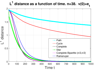
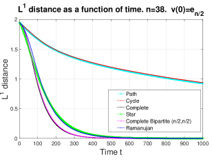
Figure 3: Comparison of the $L^{1}$ convergence for the Path, Cycle, Complete, Star, Complete Bipartite graphs and for a relatively sparse expander graph, each on 38 nodes. The left and right figures differ only where we place the starting weight 1 (all other starting weights are 0: On the left figure we place the 1 in the middle of the star and the side of the path, on the right in the middle of the path and on a terminal node of the star; the other graphs are symmetric.

3.2.2 Improved bounds: $\alpha$-covering, flow and comparison techniques.

In this section we introduce new techniques to bound $t_{\epsilon,1}$ for several instances. These bounds will add information not derivable from Theorems 1 or 4. Our first very simple but also very useful observation will be that the worst initialization always happens at a corner of the $L^{1}$-unit ball. Our proof uses the convexity of the $L^{1}$ norm together with a coupling argument.

Definition 4 ($L^{1}$-unit ball $\Diamond$).

The $L_{1}$-unit ball is the set

$$\Diamond_{n}=\{v\in\mathbb{R}^{n}\mid||v||_{1}\leq 1\}$$

When $n$ is clear from the context, we just write $\Diamond$ for $\Diamond_{n}$.

We have:

Proposition 1.

$\Diamond_{n}$ is the convex hall of $\{e_{1},\ldots,e_{n},-e_{1},\ldots,-e_{n}\}$.

Lemma 7.

The mixing properties of the process do not change if we replace $v(0)$ with $-v(0)$.

Theorem (Theorem 2 in Section 1).

Let $G$ be a graph with $n$ nodes. For every fixed $t$, define $v_{{\rm slowest},t}$ such that $\mathbb{E}\lVert v(t)-\bar{v}\rVert_{1}$ is maximized (if there are more than one such starting vectors we can non-deterministically pick one). Then we can define

$$v_{{\rm slowest},t}=e_{i}=(0,\cdots,0,\underbrace{1}_{i},0,\cdots,0)\;\;\;\;{\rm for}\;{\rm some}\;1\leq i\leq n$$

The theorem follows from Proposition 1, Lemma 7 and from the following fact:

Proposition 2.

Assume that $v$ is a convex combination of $v_{1},\ldots,v_{\ell}$, i.e. $v=\sum_{i=1}^{\ell}\lambda_{i}v_{i}$, where $\sum_{i=1}^{\ell}\lambda_{i}\;=\;1$ and $\lambda_{i}\geq 0$ for $1\leq i\leq\ell$. Let $v(t)$, respectively $v_{i}(t)$ denote state vector when we start from $v$, respectively from $v_{i}$ ($1\leq i\leq\ell$). Then

$$\mathbb{E}(\lVert v(t)-\bar{v}\rVert_{1})\;\leq\;\sum_{i=1}^{\ell}\lambda_{i}\;\mathbb{E}(\lVert v_{i}(t)-\bar{v}\rVert_{1})$$

Proof.

We couple two processes. The first process is simply the averaging process with initial vector $v$, while the second process has a random initialization, which equals $v_{i}$ with probability $\lambda_{i}$ ($1\leq i\leq\ell$). After specifying the initial vector, we always choose the same edge for both processes at every step. After $t$ steps, we observe that

$$\lVert v(t)-\bar{v}\rVert_{1}\;=\;\left\lVert\sum_{i=1}^{n}\lambda_{i}(v_{i}(t)-\bar{v}_{i})\right\rVert_{1}\;\;\leq\;\sum_{i=1}^{n}\lambda_{i}\left\lVert v_{i}(t)-\bar{v}_{i}\right\rVert_{1}$$

taking expectation on both sides yields

$$\mathbb{E}\lVert v(t)-\bar{v}\rVert_{1}\leq\sum_{i=1}^{n}\lambda_{i}\mathbb{E}\;\lVert v_{i}(t)-\bar{v}_{i}\rVert_{1}\;,$$

as desired. ∎

Proof.

(of theorem 2) From the above theorem we get that when $v$ is a convex combination of $v_{i}$s, then $\mathbb{E}\lVert v(t)-\bar{v}\rVert_{1}\;\leq\;\max_{i=1}^{\ell}\mathbb{E}\;\lVert v_{i}(t)-\bar{v}_{i}\rVert_{1}$. Assume now that $\lVert v\rVert=1$. Since $v$ is a convex combination of the $e_{i}$s and $-e_{i}$s, there must be an $i$ such that either $\mathbb{E}\lVert v(t)-\bar{v}\rVert_{1}\;\leq\;\mathbb{E}\lVert e_{i}(t)-\frac{1}{n}{\bf 1}\rVert_{1}$ or $\mathbb{E}\lVert v(t)-\bar{v}\rVert_{1}\;\leq\;\mathbb{E}\lVert-e_{i}(t)-\frac{1}{n}{\bf 1}\rVert_{1}$. But since both right hand sides are the same, for $v_{{\rm slowest},t}$ we can pick the $e_{i}$ with the positive sign, and Theorem 2 follows. ∎

Finding the slowest initialization requires knowing the structure of the underlying graph. For example, by vertex transitivity, every $v(0)=e_{i}$ $(1\leq i\leq n)$ converges at the same speed for complete graphs and cycles. On the other hand, it is not hard to show that for star graphs starting from a leaf is strictly slower than starting from the root.

Now we can assume without loss of generality that the process starts at a corner of the simplex. We give some techniques to bound the $L^{1}$ mixing, which improves the general bound in Theorem 4.

3.2.2.1 $\alpha$-covering

The $\alpha$-cover time captures the first time that at least $\alpha$-proportion of the entries of $v(t)$ are non-zero.

Definition 5 ($\alpha$-covering time).

For any vector $v\in\mathbb{R}^{n}$, let $n(v)\equiv\#\{i:v_{i}\neq 0\}$ denote the number of non-zero components of $v$. Suppose the averaging process starts at $v(0)=e_{i}$. We denote by $t_{\text{cov}}(\epsilon,i):=\mathbb{E}[\inf\{t:n(v(t))=\epsilon n,v(0)=e_{i}\}]$ the expected time that $v(t)$ has $\alpha n$ non-zero coordinates when starting from $e_{i}$. We also define the $\alpha$-covering time as $t_{\text{cov}}(\alpha):=\max_{i}t_{\text{cov}}(\alpha,i).$

The notion comes from [Chatterjee et al., 2021], where it was observed that the $\alpha$-covering time gives a “makeshift” lower bound for the $L^{1}$-mixing time of $K_{n}$. In general:

Proposition 3 (Alternative lower bound on $t_{\epsilon,1}$).

$$t_{\epsilon,1}\geq t_{\text{cov}}(1-\epsilon).$$

(See the easy proof in Section 6.3.3.1.) The quantity $t_{\text{cov}}(1-\epsilon)$ can often be calculated or bounded by coupon-collector type arguments. For example, $t_{\text{cov}}(1-\epsilon)$ is at least $\Theta_{\epsilon}(n\log n)$ if the graph is nearly regular:

Proposition 4.

Let $G_{n}$ be a graph with $n$ nodes which satisfies: $\frac{\max_{i}d_{i}}{\min_{i}d_{i}}\leq C$ for some universal constant $C$, where $d_{i}$ is the degree of node $i$. Then $t_{\text{cov}}(1-\epsilon)\geq\frac{n}{2C}\log((1-\epsilon)n).$

Proposition 5 (Expander graph).

Let $G_{n}$ be a be a family of bounded degree regular expander graphs with $n$ nodes. Then $t_{\text{cov}}(1-\epsilon,\;G_{n})=\Theta_{\epsilon}(n\log n)$.

The proofs of the above propositions are in Sections 6.3.3.2 and 6.3.3.3.

Although $t_{\text{cov}}(1-\epsilon)$ never beats our best bounds on $t_{\epsilon,1}$, and it fails to give good bounds for graphs like e.g. the star graph, it often gives an easy-to-prove approximation, and it is applicable to various averaging processes with different weight updates, not just ours.

3.2.2.2 Flow

The averaging process is a transportation process, and observing the mass flow can be a way to estimate the mixing time. A typical example is the path graph $P_{n}$ with $n$ points. Assuming we label the nodes by $1,2,\dots,n$ from left to right, and initialize the process from the leftmost entry. It is clear that the direction of the flow is always from left to right at every step, see Figure 4 for illustrations. Lower bounds on the flow at each step can be translated to new upper bounds for the $L^{1}$ convergence. The flow technique is based on the next general proposition:

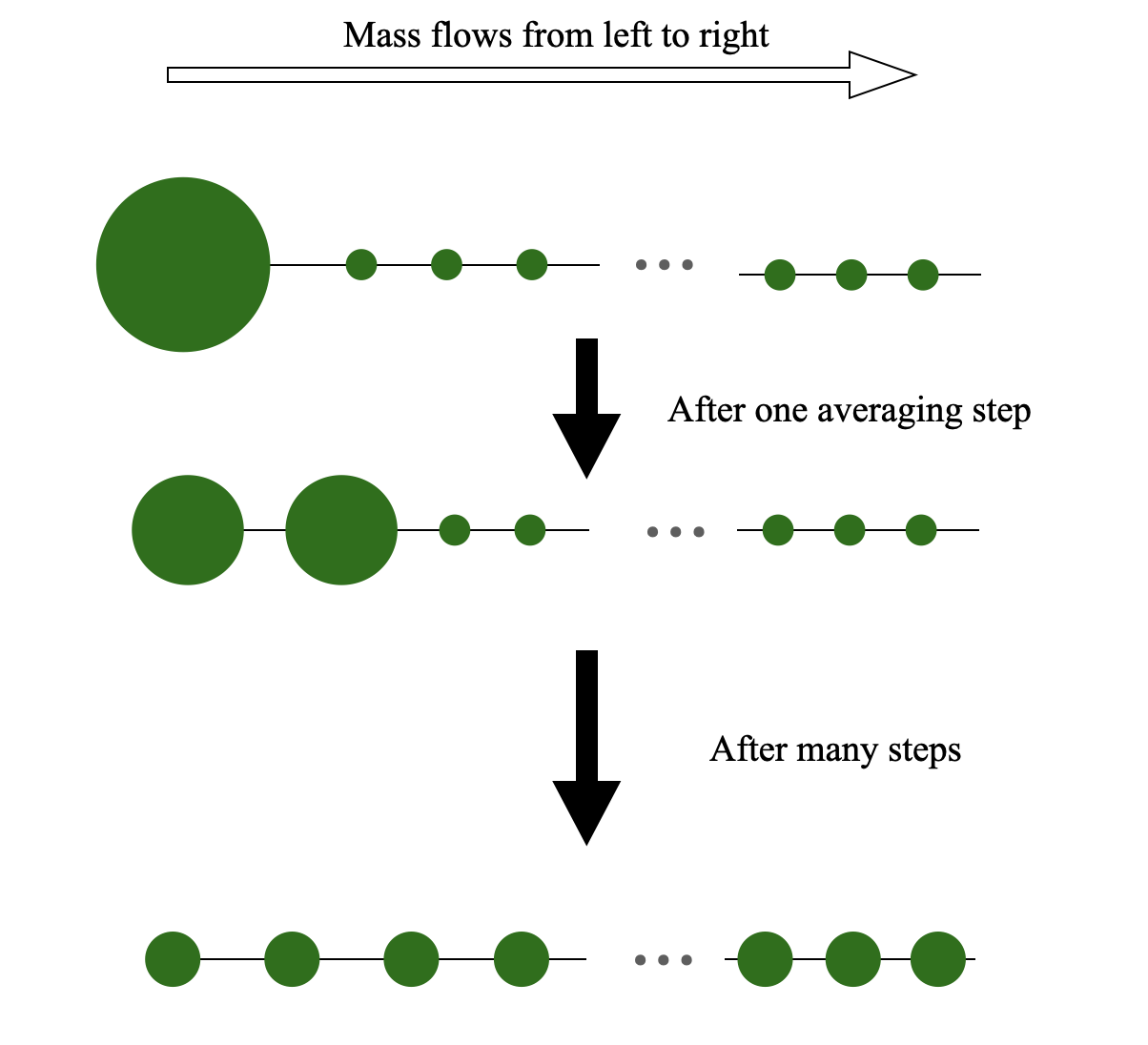
Figure 4: An illustrative figure for the mass flow on the path graph $P_{n}$.

Proposition 6 (Upper bounding $t_{\epsilon,1}$ via the flow technique).

Let $G$ be a connected undirected graph. For a starting vector $v(0)$ of the averaging process on $G$ define $\bar{v}:=\bar{v}(0)$. Suppose that for any $v(0)$ with $\lVert v(0)\rVert\leq 1$ and each $t\geq 1$ there exists a non-negative real-valued random variable $F(t,v(0))$ (called flow) over the random edge sequences of length $t$ such that

• There exists a $C>0$ such that for every $v(0)$ with $\lVert v(0)\rVert\leq 1$ and every $t\geq 1$ and every $w\in\mathbb{R}^{V(G)}$ we have:

  $$\mathbb{E}[F(t,v(0))\mid v(t-1)=w]\geq C\,\lVert w-\bar{v}\rVert_{1}$$

• The cumulative flow, $\sum_{t}F(t,v(0))$, on the space of infinite random edge sequences, converges to a random variable $F(v(0))$ in $L^{1}$, i.e., $\mathbb{E}[\lVert\sum_{t=1}^{k}F(t,v(0))-F(v(0))\rVert]\rightarrow 0$ as $k\rightarrow\infty$.

Let $\mathbb{E}_{\rm max}=\max_{\lVert v(0)\rVert\leq 1}\mathbb{E}[F(v(0))]$. Then the mixing time can be upper-bounded by

$$t_{\epsilon,1}(G,v(0))\leq\frac{8\,\mathbb{E}[F(v(0))]}{\epsilon^{2}\,C};\;\;\;\;t_{\epsilon,1}(G)\leq\frac{8\,\mathbb{E}_{\rm max}}{\epsilon^{2}\,C}$$

where $t_{\epsilon,1}(G,v(0))\equiv\min\left\{t\in\mathbb{N}\;\middle|\;\mathbb{E}\left[\lVert v(t)-\bar{v}(0)\rVert_{1}\right]\leq\epsilon\right\}$.

Proof.

Fix an initialization with $\lVert v(0)\rVert\leq 1$ and for simplicity let us omit $v(0)$ from the arguments of $F(t)$ and $F$. Let $E(t)$ be the event $\{\lVert v(t)-\bar{v}\rVert_{1}\geq\frac{\epsilon}{2}\}$. Then we have

$$\frac{\epsilon}{2}\mathbb{P}[E(t)]\;\leq\;\mathbb{E}[\lVert v(t)-\bar{v}\rVert_{1}]\leq\frac{\epsilon}{2}+2\mathbb{P}[E(t)]$$ (15)

The last inequality is due to $\lVert v(t)-\bar{v}\rVert_{1}\leq\lVert v(t)\rVert_{1}+\lVert\bar{v}\rVert_{1}\leq 2$. To bound $\mathbb{P}[E(t)]$, we observe:

$$\mathbb{E}[F]\;=\;\mathbb{E}\left[\sum_{l=1}^{\infty}F(l)\right]\;\geq\;\mathbb{E}\left[\sum_{l=1}^{t}F(l)\right]\;\geq\;\frac{\epsilon\,C}{2}\sum_{l=1}^{t}\mathbb{P}\left[E(l-1)\right]\;\geq\;t\frac{\epsilon\,C}{2}\mathbb{P}\left[E(t-1)\right],$$

where the last inequality uses the fact $E(t)\subset E(t-1)\subset E(t-2)\cdots$, and the second to last inequality uses the left side of Equation (15). Our result follows when taking $t\geq\frac{8\mathbb{E}[F]}{\epsilon^{2}C}$, plugging in the result to the right-side inequality of (15), and maximizing over all $\lVert v(0)\rVert\leq 1$. ∎

Remark 1.

The conditional random variable $F(t,v(0),w):=[F(t,v(0))\mid v(t-1)=w]$ will only depend on $w$ and the last edge picked, but is independent on $t$ and $v(0)$. Thus we can uniquely define $F^{\prime}(w):=F(t,v(0),w)$. Of course, $F(t,v(0))$ must also dependent on the probabilities $\mathbb{P}(v(t-1)=w)$.

Now we use the flow technique to analyze the path graph. Notice that Theorem 4 shows $t_{\epsilon,1}(P_{n})$ is between $\Theta_{\epsilon}(n^{3})$ and $\Theta_{\epsilon}(n^{3}\log n)$.

Proposition 7 (Path graph).

The $L^{1}$ mixing time for the path graph equals $\Theta_{\epsilon}(n^{3})$ when the initialization vector $v(0)=e_{1}$.

Proof.

It follows from induction that the random vector $v(t)$ is monotone in the sense that $v_{i}(t)\geq v_{j}(t)$ when $i\leq j$. We define $F(t)$ as $\frac{v_{I}(t)-v_{I+1}(t)}{2}$ where $(I,I+1)$ is the random edge chosen at time $t$ (since $v(0)$ is fixed, we omit it from the argument list of $F(t,v(0))$). Here $F(t)$ is the mass transported from left to right at time $t$. Given vector $v(t-1)$, the conditional expectation of $F(t)$ equals

$$\mathbb{E}[F(t)\mid v(t-1)]=\frac{v_{1}(t-1)-v_{n}(t-1)}{2(n-1)}\geq\frac{\lVert v(t-1)-\bar{v}\rVert_{1}}{2n(n-1)},$$

therefore the quantity $C(n)$ in Proposition 6 can be chosen as $1/(2n^{2}-2n)$. On the other hand, due to the convergence theorem, the long-time total cumulative flow across all the edges is $\sum_{k=1}^{n-1}1-\frac{k}{n}=(n-1)/2$. Therefore $\mathbb{E}[F_{n}]=\frac{n-1}{2}$. Applying Proposition 6 gives us the mixing time upper bound $\frac{8n(n-1)^{2}}{\epsilon^{2}}$. ∎

3.2.2.3 Comparison and splitting:

The comparison idea has been widely used in analyzing Markov chains Diaconis and Saloff-Coste [1993b], Diaconis and Saloff-Coste [1993a] to get sharp results on the mixing time. Here we develop comparison techniques to prove the mixing time for the averaging process. Our results can be applied to show that the process mixes in $\Theta(n^{3})$ steps on both Dumbbell graphs $D_{n}$ and cycles $C_{n}$. When studying the mixing on Dumbbell graphs, we compare the averaging process with the same process on the complete graph $K_{n}$. When studying the mixing on cycles, we compare the process with a new splitting process and use the results in Proposition 7.

The Dumbbell graph.

The Dumbbell graph $D_{n}$ on $2n$ nodes is a disjoint union of two complete graphs of size $n$, connected by an edge.

Theorem 6.

The $\epsilon$-mixing time of the Dumbbell graph is $\Theta_{\epsilon}(n^{3})$.

Proof Sketch of Theorem 6.

(See the detailed proof in Section 6.3.3.4.) Let the complete graph on $\{1,\ldots,n\}$ be denoted by $L$, and the complete graph on $\{n+1,\ldots,2n\}$ be denoted by $R$. We also call edge $e=(n,2n)$ a bridge. We shall decompose the edge sequence of the process to subsequences, separated by those events when $e$ is picked. We call the run of each subsequence a phase, while averaging over the edge $e$ an equalization step.

We may assume without loss of generality that the initialization vector is $e_{1}$. Easily deducible from the random edge sequence, each phase takes a random time which is geometrically distributed with expectation $\Theta(n^{2})$. It is known from both Theorem 4 and [Chatterjee et al., 2021] that the mixing time of the complete graph is $\Theta(n\log n)$ which is smaller than $\Theta(n^{2})$. Therefore we expect each phase very close to equalizing half of the Dumbbell graph, and each equalization step transfers $\Theta(1/n)$ mass from one part to the other. Therefore, it takes in total $\Theta(n)$ phases, and in turn $\Theta(n^{3})$ steps for mixing. ∎

The Cycle graph.

Let $C_{n}$ be the cycle graph on $n$ nodes. The usual spectral argument gives $\Theta(n^{3})\leq t_{\epsilon,1}\leq\Theta(n^{3}\log n)$, and our goal is to sharpen this to $t_{\epsilon,1}(C_{n})=\Theta(n^{3})$. The proof sketch that we present here is discussed in more details in Section 6.3.3.5. It has two main ideas: the flow idea for the path graph $P_{n}$, and an interesting application of the comparison method.

Let $PC_{1}$ denote the original averaging process on $C_{n}$. We also define a new splitting process, $PC_{2}$. The process starts at a vector $v(0)=(v_{1},v_{2},\cdots,v_{n})^{T}$ with $v_{1}\geq v_{2}\geq\cdots\geq v_{n}$. Then, in each step $PC_{2}$ proceeds as follows:

 

• Chooses an edge $(i,i+1\mod n)$ uniformly at random.

• When $i<n$, updates both $v_{i}$ and $v_{i+1}$ to $\frac{v_{i}+v_{i+1}}{2}$.

• When $i=n$, if $\frac{v_{1}+v_{n}}{2}\geq v_{2}$, updates the sequence to $(\frac{v_{1}+v_{n}}{2},\frac{v_{1}+v_{n}}{2},v_{2},v_{3},\cdots v_{n-1})$. Otherwise, let $k\geq 2$ be the largest index with $v_{k}>\frac{v_{1}+v_{n}}{2}$, splits the original sequence into two sequences

  $$\left(\underbrace{\frac{v_{1}+v_{n}}{2},\frac{v_{1}+v_{n}}{2},\dots,\frac{v_{1}+v_{n}}{2}}_{k+1},v_{k+1},\dots,v_{n-1}\right)$$

  and

  $$\left(v_{2}-\frac{v_{1}+v_{n}}{2},v_{3}-\frac{v_{1}+v_{n}}{2},\dots,v_{k}-\frac{v_{1}+v_{n}}{2},\underbrace{0,0,\dots,0}_{n-k+1}\right)$$

  and proceeds the splitting process $PC_{2}$ on the two sequences independently.

 

Unlike the averaging process, the splitting process may split one sequence into many sequences after $t$ steps. On the other hand, as long as the process starts at a non-increasing sequence, in the splitting process monotonicity will be preserved for every split sequence, and for every time step $t$.

First we define a few notations. Consider the splitting process with a non-increasing initialization $v=v(0)$. For time $t$, let $N_{t}$ be the number of sequences from the splitting process ($N_{t}$ is a random variable), and denote by $v^{1}(t),\cdots,v^{N_{t}}(t)$ those sequences. We also let $\tilde{v}(t):=\sum_{i=1}^{N_{t}}v^{i}(t)$ to be the sum of the split sequences, and define

$$T_{v}(t):=\lVert v(t)-\overline{v}\rVert_{1}\;\;({\rm for}\;PC_{1});\;\;\;\tilde{T}_{v}(t):=\sum_{i=1}^{N_{t}}\lVert v^{i}(t)-\overline{v^{i}}(t)\rVert_{1}\;\;({\rm for}\;PC_{2})$$

In Section 6.3.3.5 we show:

Lemma 8.

Let $PC_{1}$ and $PC_{2}$ processes as above with the same initialization $v=(v_{1},v_{2},\cdots,v_{n})$ satisfying $v_{1}\geq v_{2}\geq\cdots\geq v_{n}$. We have:

$$\mathbb{E}[T_{v}(t)]\leq\mathbb{E}[\tilde{T}_{v}(t)]$$

and

$$\tilde{T}_{v}(t)\leq n(\tilde{v}_{1}(t)-\tilde{v}_{n}(t))\;\;\;\;\;{\rm where}\;\tilde{v}_{j}(t):=\sum_{i=1}^{N_{t}}v^{i}_{j}(t)$$

Due to vertex transitivity, without loss of generality we assume that $v=e_{1}=(1,0,\cdots,0)^{T}$ is the initial vector. We define the linear form $Q(\vec{x})=\sum_{i=1}^{n}(n+1-i)x_{i}$ and introduce $\tilde{Q}(t)=Q(\tilde{v}(t))$. Then we follow how $\tilde{Q}(t)$ changes throughout the splitting process $PC_{2}$. We show that $\tilde{Q}(t)$ is monotonically non-increasing in $t$ and give a lower bound on its conditional expected change in one step:

Lemma 9.

Let $v=e_{1}$ be the initial vector. With all the notations defined above, we have:

$$n=\tilde{Q}(1)\geq\tilde{Q}(2)\geq\cdots\geq\tilde{Q}(t)\geq\cdots\geq 0\;\;\;\;\mbox{(over every fixed infinite edge sequence)},$$

and

$$\mathbb{E}[\tilde{Q}(t-1)-\tilde{Q}(t)\mid\tilde{v}(t-1)]\geq\frac{\tilde{v}_{1}(t-1)-\tilde{v}_{n}(t-1)}{2n}\;.$$

Lemma 8 asserts that we can use the mixing time of the splitting process $PC2$ to upper bound the original process $PC1$. Notice that $\tilde{Q}(1)=n$, and that $\tilde{Q}(t)$ always remains non-negative. The total decrease of $\tilde{Q}$ throughout the entire process is therefore upper bounded by $n$ (in every branch of the process). Let $E(t)$ be the event that $\tilde{v}_{1}(t)-\tilde{v}_{n}(t)\geq\epsilon/2n$. It suffices to show, that $\mathbb{P}[E(t)]\leq\epsilon/4$ for $t=\Theta_{\epsilon}(n^{3})$ (here we used the second part of Lemma 8). The second equation in Lemma 9 shows

$$\mathbb{E}[\tilde{Q}(t-1)-\tilde{Q}(t)]\geq\frac{\epsilon}{4n^{2}}\mathbb{P}[E(t-1)]$$

by only counting the contribution made by the vectors in $E(t-1)$. Summing the above inequality from $t=1$ to $t=16n^{3}/\epsilon^{2}$, and observing the fact that $E(t)\subseteq E(t-1)\subseteq E(t-2)\subseteq\cdots$, we have

$$n\geq\frac{16n^{3}}{\epsilon^{2}}\frac{\epsilon}{4n^{2}}\mathbb{P}[E(16n^{3}/\epsilon^{2})],$$

and therefore $\mathbb{P}[E(16n^{3}/\epsilon^{2})]\leq\frac{\epsilon}{4}$, which shows our main theorem (details are in Section 6.3.3.5):

Theorem 7 (Mixing time on a cycle).

$t_{\epsilon,1}(C_{n})=\Theta_{\epsilon}(n^{3})$.

3.3 $L^{2}\rightarrow L^{1}$ convergence

In this section we study $L^{1}$ convergence with respect to the initialization $\lVert v(0)\rVert_{2}=1$. Since the $L^{2}$ unit sphere, where the initial vector ranges, contains the $L^{1}$ unit sphere, but we measure the convergence in the $L^{1}$ distance, we must have slower (or at most equal) convergence than in the $L^{1}\rightarrow L^{1}$ case:

Proposition 8.

Let $G$ be any connected graph with $n$ nodes, we have $t_{\epsilon,1}\leq t_{\epsilon,2\rightarrow 1}$

Theorem 3 implies the proposition below (the simple details of the implication are in 6.4.2):

Proposition 9.

Let $v(0)$ be an arbitrary vector on $\mathbb{R}^{n}$ and $\bar{v}$ as before. Then the $L^{1}$ distance between $v(t)$ and $\bar{v}$ satisfies:

$$\mathbb{E}[\lVert v(t)-\bar{v}\rVert_{1}]\leq\bigg{(}1-{1\over 2\gamma(G)}\bigg{)}^{t/2}\sqrt{n}\;\lVert v(0)-\bar{v}\rVert_{2}$$ (16)

Furthermore, the slowest convergence speed is at least $\left(1-\frac{1}{2\gamma(G)}\right)^{t}$:

$$\sup_{\left\|v(0)\right\|_{2}=1}\mathbb{E}[\left\|v(t)-\bar{v}\right\|_{1}]\geq\left(1-\frac{1}{2\gamma(G)}\right)^{t}.$$

Proposition 9 gives the following general upper and lower bounds for $t_{\epsilon,2\rightarrow 1}$ that are very similar to formulas in Theorem 4 (proof details are in 6.4.3):

Corollary 6 (General bounds for $t_{\epsilon,2\rightarrow 1}$).

$$(2\gamma(G)-1)\log(\epsilon^{-1})\leq t_{\epsilon,2\rightarrow 1}\leq 4\gamma(G)\log(\sqrt{n}\epsilon^{-1})$$ (17)

In particular, for every undirected connected graph with $n\geq 3$ nodes, we have

$$\gamma(G)\log(\epsilon^{-1})\leq t_{\epsilon,2\rightarrow 1}\leq 4\gamma(G)\log(\sqrt{n}\epsilon^{-1})$$ (18)

The $\log n$ gap between the lower and upper bounds in Corollary 6 essentially comes from the Cauchy-Schwarz inequality used to prove Proposition 9. The gap however can be removed when $L(G)$ has a delocalized Fiedler vector.

Definition 6.

A vector $v\in\mathbb{R}^{n}$ is called $\delta$-delocalized if

$$\lVert v\rVert_{1}\geq\delta\sqrt{n}\>\lVert v\rVert_{2}\;.$$ (19)

Heuristically, a vector is called delocalized if the top constant fraction of its coordinates are of roughly the same magnitude (there are other ways to quantify delocalization, but they are of similar spirit). Delocalization of eigenvectors of graph Laplacians is an active area in random matrix theory and combinatorics. We refer the readers to Brooks and Lindenstrauss [2013] and Rudelson and Vershynin [2015] for recent progress. We show, that $\Theta(\log(n)\gamma(G))$ is the correct magnitude for $t_{\epsilon,2\rightarrow 1}$ given the second eigenvector of the graph Laplacian is $\Omega(1)-$delocalized. Proof details can be found in Section 6.4.4.

Theorem 8 (Improved bounds for $t_{\epsilon,2\rightarrow 1}$ with delocalized eigenvector).

Let $G$ be an undirected connected graph with $n$ nodes. Let $u_{2}$ be a unit eigenvector of $L(G)$ with respect to the second smallest eigenvalue. If $u_{2}$ is $\delta$-delocalized, we have:

$$\left(2\gamma(G)-1\right)\log(\delta\sqrt{n}\epsilon^{-1})\leq t_{\epsilon,2\rightarrow 1}\leq 4\gamma(G)\log(\sqrt{n}\epsilon^{-1})$$ (20)

In particular, for every undirected connected graph with $n\geq 3$ nodes, we have

$$\gamma(G)\log(\delta\sqrt{n}\epsilon^{-1})\leq t_{\epsilon,2\rightarrow 1}\leq 4\gamma(G)\log(\sqrt{n}\epsilon^{-1})$$ (21)

Theorem 8 can be used to analyze the $L^{2\rightarrow 1}$ mixing time for several natural families of graphs. Our results are summarized in Table 3 below (see Section 6.4.5 for proof details).

Graph	Complete graph $K_{n}$	Binary tree $B_{n}$	Star $S_{n-1}$	Cycle $C_{n}$
$\boldsymbol{t_{\epsilon,2\rightarrow 1}}$	$\Theta_{\epsilon}(n\log n)$	$\Theta_{\epsilon}(n^{2}\log n)$	$\Theta_{\epsilon}(n\log n)$	$\Theta_{\epsilon}(n^{3}\log n)$

Table 3: The $L^{2\rightarrow 1}$ mixing time for selected graphs

4 Numerical Explorations

The goal of this section is to numerically corroborate some of the theory and inspire future work. We explore the expected $L^{1}$ behavior for three distinct scenarios: (1) The complete graph (2) Star graph with the initialization on the center (i.e., high degree) node (3) Star graph with the initialization on a leaf (i.e., high degree) node.

Fig. 5 shows the expected $L^{1}$ convergence over $20$ runs enveloped by the standard of deviation. The enveloping curves can be seen as horizontal error bars. Fig. 7 illustrates the convergence in each case as a function of the size of the graph.

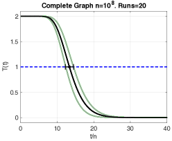
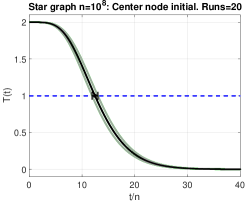
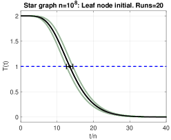
Figure 5: Expected $L^{1}$ enveloped by the standard of deviation over $20$ runs.

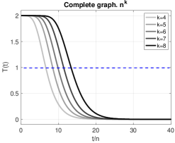
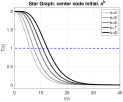
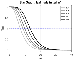
Figure 6: Convergence in time for various graph sizes.

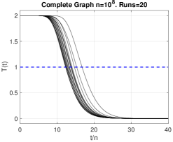
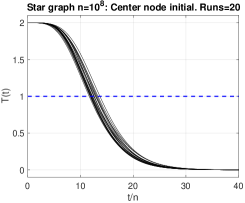
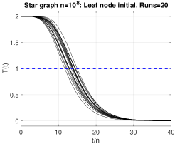
Figure 7: Convergence in time for various graphs and $20$ distinct runs per graph.

5 A related random process and the extremal nature of the complete graph with respect to it

It is shown in Corollary 5 that the complete graph has asymptotically the smallest $L^{1}$-mixing time among all undirected, connected graphs when the number of nodes goes to infinity. However, for a fixed number of nodes $n$ and a fixed number of iterations $t$, there exists other graphs that mix faster than the complete graph. For example, Figure 3 shows the star graph mixes faster than the complete graph when the number of iterations is small. In this section, we introduce a related process for which we will prove that the complete graph is extremal. The new process will be identical to the original, slowed down by a factor of $|E(G)|/{n\choose 2}$.

Given an undirected and connected graph $G$ with $n$ vertices, the new process is defined as follows: The process starts from an initial vector $v_{0}\in\mathbb{R}^{n}$. At each discrete time-step the process picks a pair of nodes $(i,j)$ uniformly at random from all ${n\choose 2}$ pairs of nodes with $i\neq j$, and performs the averaging step if $(i,j)\in E(G)$. If $(i,j)\notin E(G)$, the process simply keeps the current $v$ (i.e. it “does nothing”).

The new process clearly coincides with the original one for the complete graph, $K_{n}$. It however runs slower on general graphs $G$, due to the steps when it idles (that constitute $1-|E(G)|/{n\choose 2}$ fraction of steps, on expectation).

5.1 $L^{1}$-norm is monotonically non-increasing

Recall that if $(i,j)\in E(G)$, we update the vector $(v_{1},\dots,v_{i},\dots,v_{j},\dots,v_{n})$ by replacing $v_{i}$ and $v_{j}$ by $\frac{v_{i}+v_{j}}{2}$. The only stationary state of the process is the vector $\bar{v}=(a,a,\dots,a)^{T}$. We define

$$T_{G}(t)=\sum_{j=1}^{n}|v_{j}(t)-a|$$

where we have put the graph $G$ as subscript on purpose. By applying the averaging process to the $i^{\rm th}$ and $j^{\rm th}$ entry when $(i,j)\in E(G)$, we obtain

$$T_{G}(t+1) = T_{G}(t)-|v_{i}(t)-a|-|v_{j}(t)-a|+2\;\left|\frac{v_{i}(t)+v_{j}(t)}{2}-a\right|\;\leq\;T_{G}(t)$$

(The above argument is same for the original process and the new one.) Further, $T_{G}(t+1)$ is clearly the same as $T_{G}(t)$, when the $(i,j)$ pair picked is not in $E(G)$. Thus monotonicity holds in the case of the new process too.

5.2 The complete graph is extremal for the new process

We now prove that the complete graph converges to the averaging vector fastest in $L^{1}$ distance under the new dynamics, i.e. for any connected graph $G$ with $n$ nodes and for $K=K_{n}$ we have $\mathbb{E}_{v}\left[T_{K}(t)\right]\leq\mathbb{E}_{v}\left[T_{G}(t)\right]$ for any initialization $v$. This will in turn imply that for all $t$.

$$\sup_{\lVert v\rVert_{1}=1}\mathbb{E}_{v}\left[T_{K}(t)\right]\leq\sup_{\lVert v\rVert_{1}=1}\mathbb{E}_{v}\left[T_{G}(t)\right]$$

This implies that if we start the new process with the same initial vector, $v$, on $K_{n}$, respectively on some other graph on $n$ nodes, then after step $t$ the state vector for the complete graph will be closer to $\bar{v}$, than the corresponding state vector for the other graph (in terms of the expected distance). That is, the complete graph mixes the fastest in a strong sense.

Theorem 9.

(The complete graph is extremal) Let $G_{n}$ be any connected graph with $n$ nodes and $K=K_{n}$ be the $n$-node complete graph. Let $v$ be an arbitrary initial vector. We have $\mathbb{E}_{v}[T_{K}(t)]\leq\mathbb{E}_{v}[T_{G}(t)]$ for all $t\geq 0$ and any connected graph $G$, where expectation is with respect to the sequence of random choices of pair of nodes $1\leq i<j\leq n$.

Proof.

Let $v(0):=v=(v_{1},\dots,v_{n})$ be an arbitrary initial vector for both processes, and let $v_{K}(t)$ and $v_{G}(t)$ be the state vectors for $K=K_{n}$ and $G$, respectively, at time $t$ of the process. We prove the theorem by induction on $t$.

Case $t=0$: The statement is trivial, since $T_{K}(0)=T_{G}(0)=||v(0)-\bar{v}||_{1}$.

Inductive step: We prove $\mathbb{E}[T_{K}(t)]\leq\mathbb{E}[T_{G}(t)]$ by conditioning on the first step, and relying on $\mathbb{E}_{v}[T_{K}(t-1)]\leq\mathbb{E}_{v}[T_{G}(t-1)]$ for all $v\in\mathbb{R}^{n}$, as given by the induction hypothesis. If in the first step a pair $(i,j)\in E(G)$ is picked, then $v(1)$ is the same for both graphs and we have reduced the number of steps by one. The proof, conditioned on this event, becomes a trivial consequence of the induction hypothesis.

Next suppose, that in the first step an $(i,j)\not\in E(G)$ is picked. Without loss of generality let us assume that $(i,j)=(1,2)$. We have:

$$v_{K}(1)\;=\;v_{1,2}\;=\;\left(\frac{v_{1}+v_{2}}{2},\frac{v_{1}+v_{2}}{2},v_{3},\dots,v_{n}\right),$$

whereas $v_{G}(1)=v(0)=v$. Observe that

$$v_{1,2}=\frac{1}{2}(v_{1},v_{2},v_{3,}\dots,v_{n})+\frac{1}{2}(v_{2},v_{1},v_{3},\dots,v_{n}).$$

Now by the convexity lemma proved in Section 6.1 we have that

$$\mathbb{E}_{v_{1,2}}\left[T_{K}(t-1)\right]\leq\frac{1}{2}\mathbb{E}_{(v_{1},v_{2},v_{3,}\dots,v_{n})}\left[T_{K}(t-1)\right]+\frac{1}{2}\mathbb{E}_{(v_{2},v_{1},v_{3,}\dots,v_{n})}\left[T_{K}(t-1)\right].$$

By the symmetry of the complete graph $\mathbb{E}_{(v_{1},v_{2},v_{3,}\dots,v_{n})}\left[T_{K}(t-1)\right]=\mathbb{E}_{(v_{2},v_{1},v_{3,}\dots,v_{n})}\left[T_{K}(t-1)\right]$, so we get

$$\mathbb{E}_{v_{1,2}}\left[T_{K}(t-1)\right]\leq\mathbb{E}_{v}\left[T_{K}(t-1)\right]\;\leq\;\mathbb{E}_{v}\left[T_{G}(t-1)\right],$$

where the last inequality is by induction. Since we have considered both cases where the first randomly chosen edge is in $E(G)$ and when it is not, and in both cases the conditional expectation of $T_{K}(t)$ is less than that of $T_{G}(t)$, the proof is complete. ∎

Remark 2.

Although at first it might seem so, $T_{K}(t)\leq T_{G}(t)$ does not hold for all points of the event space, only on expectation (here we couple the processes for $K=K_{n}$ and for $G$, starting from the same vector $v$, in the obvious way, since they both run on infinite edge sequences, where the edges are taken from the complete graph). An example is furnished by the following. Let $G$ be the almost complete graph with missing edge $(1,2)$. Suppose the initial vector is $(1,0,\dots,0)$ and at the first step of the Markov chain the pair $(i,j)=(1,2)$ is picked. The state vector over the complete graph becomes $(1/2,1/2,0,\dots,0)$ and the state vector over $G$ remains to be $(1,0,\dots,0)$. Suppose that all the subsequent moves for a long time pick pairs $(i,j)$ where $i,j\neq 2$ (i.e. all moves avoid edges incident to $2$). Then after a long time the state vector over the complete graph is close to $(\text{$\frac{1}{2(n-1)}$},\frac{1}{2},\text{$\frac{1}{2(n-1)}$},\dots,\text{$\frac{1}{2(n-1)}$})$, whereas the state vector over $G$ is close to $(\frac{1}{n-1},0,\frac{1}{n-1},\dots,\frac{1}{n-1})$. Therefore, $T_{K}(t\gg 1)\approx 1-2/n$, and $T_{G}(t\gg 1)\approx 2/n$.

Remark 3.

When we compare Theorem 9 with Corollary 5, we will notice that the latter only asserts that (under the original process) the complete graph mixes fastest asymptotically, i.e. when the number of nodes goes to infinity. When $n$ is fixed and $t$ is small, the star often mixes slightly faster than the complete graph. In contrast, in the case of the new process the complete graph mixes fastest for every $t$ and $n$.

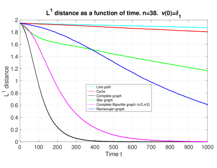
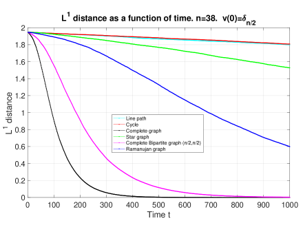
Figure 8: Numerical illustration of $L^{1}$ convergence (see Theorem 9). The two plots are different in the initialization of the state, which is mainly relevant in comparing the path and cycle graphs, and the star graph as discussed in the text. The size $n=38$ was dictated by the Ramanujan graph we picked.

5.3 Numerical illustrations for the new process

In Figure 8 we show $\mathbb{E}[T_{G}(t)]$ vs. $t=\{0,1,\dots,\tau\}$ for various graphs $G$.

6 Proofs

6.1 Preparation

In this subsection, we collect several useful results for the averaging process.

6.1.1 Averaging matrix

For a graph $G=(V,E)$ with $n$ nodes, recall that the Laplacian is defined as $L=D-A$ where $A$ and $D$ are the adjacency matrix and degree matrix of $G$ respectively. Recall that $v(t)$ is a vector-valued random variable determined by the $t^{\rm th}$ step of the averaging process. We prove a formula for the expectation of $v(t)$.

Proposition 10 (Averaging matrix).

$$\mathbb{E}[v(t)] = M^{t}v(0)\;,$$ (22)

where

$$M=I-\frac{1}{2|E|}L\;.$$ (23)

Proof.

We first prove (22) for $t=1$. Fix any index $i$, the expected value of $v_{i}(1)$ equals

$$\mathbb{E}[v_{i}(1)]=(1-\frac{d_{i}}{\lvert E\rvert})v_{i}(0)+\frac{1}{\lvert E\rvert}\sum_{(i,j)\in E}\frac{v_{i}+v_{j}}{2}\;.$$

Writing the above formula in the matrix form yields $\mathbb{E}[v(1)]=Mv(0)$, which concludes the case $t=1$. The general case follows from writing $\mathbb{E}[v(t)]$ as $\mathbb{E}\left[\mathbb{E}[v(t)\mid v(t-1)]\right]$ iteratively and using the linearity of expectation. ∎

Observe that $M$ is a doubly stochastic matrix. Assuming that the eigenvalues of $L$ are
$0=\lambda_{1}\leq\lambda_{2}\leq\cdots\leq\lambda_{n}$, the eigenvalues of $M$ are $\mu_{i}=1-\frac{\lambda_{i}}{2|E|}$ with $1\geq\mu_{1}\geq\mu_{2}\geq\cdots\geq\mu_{n}$. The eigenvalue gap of the Laplacian, $\lambda_{2}$, controls the convergence of $\mathbb{E}[v(t)]$ to the uniform distribution with respect to $t$.

6.1.2 Monotinicity and other useful properties

In this section, we will state several useful properties of the averaging process. First, the averaging process preserves linear combination, with consequences:

Proposition 11.

Let $u_{0}$, $v(0)$ be two starting vectors, $\lambda,\mu\in\mathbb{R}$ be two real numbers, $u(t),v(t)$ and $w(t)$ are results of the $t$ step averaging process with starting vectors $u_{0}$, $v(0)$ and $\lambda u_{0}+\mu v(0)$, respectively. Let $r$ be a fixed edge-sequence, i.e. a fix random branch for the process. Then

$$w(t)(r)=\lambda u(t)(r)+\mu v(t)(r)$$

As a consequence we get:

Proposition 12 (Translation and scaling).

Let $v(0)\in\mathbb{R}^{n}$ be an arbitrary initial vector, $c,\lambda\in\mathbb{R}$. Let $w_{0}=\lambda v(0)-c$ be another initial vector. Then:

$$w(t)\stackrel{{\scriptstyle\mathcal{L}}}{{=}}\lambda v(t)-c$$

where $\stackrel{{\scriptstyle\mathcal{L}}}{{=}}$ denotes equality in the distribution sense.

The proofs of Propositions 11 and 12 are straightforward and we omit them here. Proposition 12 allows us to normalize the initial vector in convenient ways, for instance when we study the $L^{2}$ norm, we can assume that the sum of the coordinates of $v(0)$ is zero and $||v(0)||_{2}=1$.

Proposition 13 (Monotonicity).

Let $f:\mathbb{R}\rightarrow\mathbb{R}$ be a convex real function. Define

$$S_{f}(v)\equiv\sum_{i=1}^{n}f(v_{i})$$

Then the sequence $S_{f}(v(i))$ $i=0,1,\ldots$ of random variables is monotonically non-increasing:

$$S_{f}(v(0))\geq S_{f}(v(1))\geq\cdots\geq S_{f}(v(t))\geq\cdots$$ (24)

Proof.

Fix any time step $k$, and assume at time $k$ an random edge $(I,J)$ is chosen, then we have

$$S_{f}(v(k+1)-S_{f}(v(k))=2f\left(\frac{v_{I}(k)+v_{J}(k)}{2}\right)-\left(f(v_{I}(k))+f(v_{I}(k))\right)\leq 0$$

where the last inequality follows from the convexity of $f$. ∎

Corollary 7.

Let $p\geq 1$. With the choice of $f(x)=\lvert x\rvert^{p}$, Proposition 13 implies that the $p$-th power of the $L^{p}$ norm of $v(t)$ is monotonically non-increasing.

6.2 Proofs for Section 3.1

6.2.1 Proof of Theorem 3

We start with the following Proposition. First notice that replacing $(v_{i},v_{j})$ by $\left(\frac{v_{i}+v_{j}}{2},\frac{v_{i}+v_{j}}{2}\right)$ decreases $S(t)=\sum_{i=1}^{n}v_{i}^{2}(t)$, the square of the $L^{2}$ norm, exactly by $(v_{i}-v_{j})^{2}/2$. Using this we show that on expectation $S(t)$ changes as:

Proposition 14.

$\mathbb{E}\left[S(t)|v(t-1)\right]=v^{T}(t-1)\,M\,v(t-1)$

Proof.

Since each edge is picked uniformly at random we have

$$S(t-1)-\mathbb{E}\left[S(t)|v(t-1)\right]=\frac{1}{|E|}\sum_{(i,j)\in E}\frac{\left(v_{i}(t)-v_{j}(t)\right)^{2}}{2}=\frac{1}{2|E|}v^{T}(t-1)\,L\,v(t-1)\;,$$

where the latter follows from the quadratic form expression of the Laplacian. Using Eq. (23) we conclude that

$$\mathbb{E}\left[S(t)|v(t-1)\right]=S(t-1)-\frac{1}{2|E|}v^{T}(t-1)\,L\,v(t-1)=v^{T}(t-1)\,M\,v(t-1)\;.$$ (25)

∎

This leads us to the upper and lower bounds about the $L^{2}$ convergence.

Proof of Theorem 3.

With no loss of generality, we take $\sum_{i=1}^{n}v_{i}(0)=0$. Since $M$ is a real symmetric matrix we write its spectral decomposition $M=\sum_{i=1}^{n}\left(1-\frac{\lambda_{i}}{2|E|}\right)u_{i}u_{i}^{T},$ where $\left(1-\frac{\lambda_{i}}{2|E|}\right)$ are the eigenvalues and $u_{i}$ are the corresponding set of orthonormal eigenvectors. $M$ is a doubly stochastic matrix that can be viewed as a transition matrix of an irreducible Markov chain. The standard Markov chain theory guarantees a unique largest eigenvalue $1$ with the corresponding eigenvector $u_{1}=\frac{1}{\sqrt{n}}(1,1,\dots,1)$. We now prove the upper and lower bound on the $L^{2}$ norm.

For the upper-bound, from Eq. (25) in Prop. 14 and the spectral decomposition of $M$ we have

$$\mathbb{E}\left[S(t)|v(t-1)\right] = \sum_{i=2}^{n}\left(1-\frac{\lambda_{i}}{2|E|}\right)|u_{i}^{T}v(t-1)|^{2}$$

$$\leq \left(1-\frac{\lambda_{2}}{2|E|}\right)\sum_{i=2}^{n}|u_{i}^{T}v(t-1)|^{2}=\left(1-\frac{\lambda_{2}}{2|E|}\right)S(t-1)\;,$$

where the first equality uses the zero-mean choice $\sum_{i=1}^{n}v_{i}(t-1)=0$. Taking an expectation of both sides with respect to $v(t-1)$ yields $\mathbb{E}[S(t)]\leq\left(1-\frac{\lambda_{2}}{2|E|}\right)\mathbb{E}[S(t-1)].$ Solving the foregoing recursion we find $\mathbb{E}[S(t)]\leq\left(1-\frac{\lambda_{2}}{2|E|}\right)^{t}\mathbb{E}[S(0)]$. Since $\mathbb{E}[S(t)]=\left\|v(t)\right\|_{2}^{2}$ we have

$$\sqrt{\mathbb{E}[\left\|v(t)\right\|_{2}^{2}]}\leq\left(1-\frac{\lambda_{2}}{2|E|}\right)^{t/2}\left\|v(0)\right\|_{2}\;.$$

For the lower-bound, we prove it by taking the initial condition to be the second eigenvector $v(0)=u_{2}$ (if there is a multiplicity, then pick any in the eigenspace). Recall that by Eq. (22) we have

$$\mathbb{E}[v(t)]=\left(1-\frac{\lambda_{2}}{2|E|}\right)^{t}u_{2}\;.$$

This along with the fact that $\left\|u_{2}\right\|_{2}^{2}=1$ give

$$\mathbb{E}[\left\|v(t)\right\|_{2}^{2}] = \sum_{i=1}^{n}\mathbb{E}\left[v_{i}^{2}(t)\right]\geq\sum_{i=1}^{n}\left(\mathbb{E}[v_{i}(t)]\right)^{2}$$

$$= \left(1-\frac{\lambda_{2}}{2|E|}\right)^{2t}\sum_{i=1}^{n}u_{2,i}^{2}=\left(1-\frac{\lambda_{2}}{2|E|}\right)^{2t}.$$

Since $u_{2}^{T}u_{1}=0$, we have that $\sum_{i=1}^{n}u_{2,i}=0$ and hence $\bar{v}=0$. The desired lower-bound then follows

$$\sup_{\left\|v(0)\right\|_{2}=1}\sqrt{\mathbb{E}[\left\|v(t)-\bar{v}\right\|_{2}^{2}]}\geq\underbrace{\sqrt{\mathbb{E}[\left\|v(t)\right\|_{2}^{2}]}}_{v(0)=u_{2}}=\left(1-\frac{\lambda_{2}}{2|E|}\right)^{t}.$$

∎

6.2.2 Proof of Corollary 1

Proof of Corollary 1.

Notice that $\left\|v(0)\right\|_{2}^{2}=\left\|v(0)-\bar{v}\right\|_{2}^{2}+\left\|\bar{v}\right\|_{2}^{2}=1$ and we have $\left\|v(0)-\bar{v}\right\|_{2}^{2}\leq 1$. Eq. (2) in the first part of Theorem 3 easily gives

$$\sqrt{\mathbb{E}[\left\|v(t)-\bar{v}\right\|_{2}^{2}]}\leq\left(1-\frac{\lambda_{2}}{2|E|}\right)^{t/2}\left\|v(0)-\bar{v}\right\|_{2}\leq e^{-\frac{t}{4|E|}\lambda_{2}}\quad,$$

where we used $\left\|v(0)-\bar{v}\right\|_{2}=1$ and $1-x\leq e^{-x}$. Solving for $t$ in $\epsilon=e^{-\frac{t}{4|E|}\lambda_{2}}$ gives the upper bound $4\gamma(G)\log(\epsilon^{-1})$ in Eq. (4).

From Eq. (3) in the second part of Theorem 3 we have

$$\sup_{\left\|v(0)\right\|_{2}=1}\sqrt{\mathbb{E}\left[\left\|v(t)-\bar{v}\right\|_{2}^{2}\right]} \geq \left(1-\frac{\lambda_{2}}{2|E|}\right)^{t}=\exp\left[t\log\left(1-\frac{\lambda_{2}}{2|E|}\right)\right]$$

$$\geq \exp\left[\frac{-t\lambda_{2}}{2|E|\left(1-\frac{\lambda_{2}}{2|E|}\right)}\right]$$

where in the last inequality we used $\log(1-x)>-x/(1-x)$. Once more solving for $t$ in $\epsilon=\exp\left[\frac{-t\lambda_{2}}{2|E|\left(1-\frac{\lambda_{2}}{2|E|}\right)}\right]$ yields the lower bound in Eq. (4)

$$t=\left(1-\frac{\lambda_{2}}{2|E|}\right)\frac{2|E|}{\lambda_{2}}\log(\epsilon^{-1})=(2\gamma(G)-1)\log(\epsilon^{-1}).$$

∎

6.2.3 Proof of the examples in Table 2

With Theorem 3 and Corollary 1 in hand, now we can estimate the $L^{2}$ convergence speed for several different graphs.

Example 1 (Complete graph).

The complete graph $K_{n}$ has $n$ nodes and $|E(K_{n})|=\frac{n(n-1)}{2}$ edges. It is well-known that the eigenvalues of the graph Laplacian $L(K_{n})$ are:

$$\lambda_{1}=0\;;\qquad\lambda_{2}=\cdots=\lambda_{n}=n\;,$$

and Theorem 3 and Corollary 1 respectively imply:

$$\bigg{(}1-\frac{1}{n-1}\bigg{)}^{t}\leq\sup_{\{v(0):\lVert v(0)\rVert_{2}=1\}}\sqrt{\mathbb{E}[\lVert v(t)-\bar{v}\rVert_{2}^{2}]}\leq\bigg{(}1-\frac{1}{n-1}\bigg{)}^{t/2},$$

and

$$(n-2)\log(\epsilon^{-1})\leq t_{\epsilon,2}(K_{n})\leq(2n-2)\log(\epsilon^{-1}).$$

Our bounds match the magnitude of the result in [Chatterjee et al., 2021, Proposition 2.1].

Example 2 (Cycle with $n$ nodes).

A cycle graph $C_{n}$ is a graph with $n$ nodes that consists of a single cycle. We know $|E(C_{n})|=n$ and the Laplacian $L(C_{n})$ can also be diagonalized explicitly, with eigenvalues $2-2\cos(kw)$ where $w\equiv\frac{2\pi}{n}$ and $0\leq k\leq\frac{n}{2}$. Since $\cos(w)=\cos(\frac{2\pi}{n})\sim 1-\frac{2\pi^{2}}{n^{2}}$ when $n$ is large, from Corollary 1 we have that $t_{\epsilon,2}(C_{n})=\Theta(n^{3})\log(\epsilon^{-1})$.

Example 3 (Star graph).

A star graph $S_{n-1}$ is a tree with $n$ nodes. It contains one root and $n-1$ leaves. We know $|E(S_{n-1})|=n-1$ and the second smallest eigenvalue of $S_{n-1}$ equals $1$. Theorem 3 and Corollary 1 imply:

$$\bigg{(}1-\frac{1}{2(n-1)}\bigg{)}^{t}\leq\sup_{\{v(0):\lVert v(0)\rVert_{2}=1\}}\sqrt{\mathbb{E}[\lVert v(t)-\bar{v}\rVert_{2}^{2}]}\leq\bigg{(}1-\frac{1}{2(n-1)}\bigg{)}^{t/2}$$

and

$$(2n-3)\log(\epsilon^{-1})\;\leq\;t_{\epsilon,2}\;\leq\;(4n-4)\log(\epsilon^{-1}).$$

Thus $t_{\epsilon,2}(S_{n-1})=\Theta(n)\log(\epsilon^{-1})$.

Example 4 (Binary tree).

A balanced full binary tree $B_{n}$ has $n-1$ edges and $\log_{2}(n+1)$ levels. It is difficult to explicitly diagonalize the graph Laplacian $L(B_{n})$, but it is well known (from the Cheeger’s inequality) that the second smallest eigenvalue $\lambda_{2}(B_{n})=\Theta(\frac{1}{n})$. More precisely, from [Guattery and Miller, 1994, Lemma 3.8] we have

$$\frac{1}{n}<\lambda_{2}(B_{n})<\frac{2}{n}\;.$$

And Theorem 3 and Corollary 1 imply:

$$\bigg{(}1-\frac{1}{n(n-1)}\bigg{)}^{t}<\sup_{\{v(0):\lVert v(0)\rVert_{2}=1\}}\sqrt{\mathbb{E}[\lVert v(t)-\bar{v}\rVert_{2}^{2}]}<\bigg{(}1-\frac{1}{2n(n-1)}\bigg{)}^{t/2}$$

and

$$(n^{2}-n-1)\log(\epsilon^{-1})\;<\;t_{\epsilon,2}\;<\;4(n^{2}-n)\log(\epsilon^{-1}).$$

Thus $t_{\epsilon,2}(B_{n})=\Theta(n^{2})\log(\epsilon^{-1})$.

6.3 Proofs for Section 3.2

6.3.1 Proof of Theorem 4

Proof of Theorem 4.

For the upper bound, Theorem 3 and Cauchy-Schwarz give:

$$\mathbb{E}[\lVert v(t)-\bar{v}\rVert_{1}] =\mathbb{E}\left[\sum_{i=1}^{n}\lvert v_{i}(t)-\bar{v}\rvert\right]\;\leq\;\sqrt{n}\;\mathbb{E}\left[\sqrt{\sum_{i=1}^{n}\lvert v_{i}(t)-\bar{v}\rvert^{2}}\;\right]$$

$$\leq\sqrt{n}\;\sqrt{\mathbb{E}[\lVert v(t)-\bar{v}\rVert_{2}^{2}]}\leq\sqrt{n}\;\bigg{(}1-{1\over 2\gamma(G)}\bigg{)}^{t/2}\lVert v(0)-\bar{v}\rVert_{2}.$$

Since $\lVert v(0)\rVert_{2}\leq\lVert v(0)\rVert_{1}=1$, we have $\lVert v(0)-\bar{v}\rVert_{2}\leq 1$. Therefore solving for $t$ in $\sqrt{n}\;\bigg{(}1-{1\over 2\gamma(G)}\bigg{)}^{t/2}=\epsilon$ gives us the upper bound in Eq. (5).

For the lower bound, we take $v(0)=u_{2}/\lVert u_{2}\rVert_{1}$ (so $\bar{v}=\vec{0}$) where $u_{2}$ is the eigenvector of $L(G)$ corresponding to $\lambda_{2}$. After the normalization it is clear that $\lVert v(0)\rVert_{1}=1$. Recall that $\mathbb{E}[v(t)]=M^{t}v(0)$, which gives:

$$\mathbb{E}[\lVert v(t)\rVert_{1}]\;\geq\; \sum_{i=1}^{n}\bigg{|}\mathbb{E}[v_{i}(t)]\bigg{|}=\;\lVert M^{t}v(0)\rVert_{1}\;=\;\bigg{\lVert}\bigg{(}1-{1\over 2\gamma(G)}\bigg{)}^{t}v(0)\bigg{\rVert}_{1}$$

$$\;= \bigg{(}1-{1\over 2\gamma(G)}\bigg{)}^{t}\geq\exp{\left[-\frac{t}{2\gamma(G)}/\left(1-\frac{1}{2\gamma(G)}\right)\right]}.$$ (26)

Again, solving for $t$ in $\exp{\left[(-\frac{t}{2\gamma(G)})/(1-\frac{1}{2\gamma(G)})\right]}=\epsilon$ gives us the lower bound in Eq.  (5). ∎

6.3.2 Remaining Proofs for Section 3.2.1 : $\Omega(n\log n)$ lower bound

6.3.2.1 Proof of Corollary 4

Proof.

The spectral properties of star (see example 7) shows the mixing time is between $\Theta(n)$ and $\Theta(n\log n)$ for every fixed $\epsilon$. Theorem 1 gives a universal $\Omega(n\log n)$ lower bound. Therefore we conclude $t_{\epsilon,1}(S_{n-1})=\Theta_{\epsilon}(n\log n)$. ∎

6.3.2.2 Proof of Corollary 5

Proof.

Proof of Corollary 5 It is known in Chatterjee et al. Chatterjee et al. [2021] that for every $2>\epsilon>0$,

$$\frac{(2\log 2)t_{1}(\epsilon,K_{n})}{n\log(n/2)}\rightarrow 1.$$

Meanwhile, we have $t_{1}(\epsilon,G_{n})\geq\frac{(1-\epsilon)}{2\log 2}n\log(n)-O(n)$ from Theorem 1. Combining the two results together and Corollary 5 immediately follows. ∎

6.3.3 Remaining Proofs for Section 3.2.2 : $\alpha$-covering, flow, comparison, and splitting

6.3.3.1 Proof of Proposition 3

Proof.

Suppose one starts at $v(0)=e_{i}$, and let $T_{\text{cov}}(1-\epsilon,i)$ be the first time $v(t)$ has $(1-\epsilon)n$ non-zero elements. Then for any $t\leq T_{\text{cov}}(1-\epsilon,i)$, we have:

$$\lVert v(t)-\bar{v}\rVert_{1}=\lVert v(t)-\frac{1}{n}\mathbf{1}\rVert_{1}\geq\epsilon n\cdot\frac{1}{n}=\epsilon,$$

which implies

$$t_{\epsilon,1}\geq\mathbb{E}[T_{\text{cov}}(1-\epsilon,i)]=t_{\text{cov}}(1-\epsilon,i).$$

Since $i$ is arbitrary, we conclude $t_{\epsilon,1}\geq t_{\text{cov}}(1-\epsilon)$. ∎

6.3.3.2 Proof of Proposition 4

Proof.

Without loss of generality we assume the process is initialized at $e_{1}=(1,0,\cdots,0)$. Let $n_{0}\equiv(1-\epsilon)n$. Let $W_{i}$ be the ‘waiting time’ of the $(i+1)$-th non-zero coordinate given the vector has $i$ non-zero coordinate. Clearly $t_{\text{cov}}(1-\epsilon)(G_{n})\geq\mathbb{E}[W_{1}+W_{2}+W_{3}+\cdots W_{n_{0}}]$.

Given the vector has $k$-non zero coordinates, the waiting time of $W_{k}$ follows a geometric distribution with success probability no larger than

$$\frac{kM}{|E(G_{n})|}\leq 2\,C\,\frac{k}{n}$$

since there are at most $kM$ edges which connects between the zero and non-zero elements. Therefore, $\mathbb{E}[W_{k}]\geq\frac{n}{2Ck}$ for every $k\leq n_{0}$, and summing up over $\mathbb{E}[W_{k}]$ yields

$$t_{\text{cov}}(1-\epsilon)(G_{n})\geq\sum_{k=1}^{n_{0}}\frac{n}{2Ck}\geq\frac{n}{C}\log(n_{0})=\frac{n}{2C}\log\left((1-\epsilon)n\right).$$

∎

6.3.3.3 Proof of Proposition 5

Proof.

It follows from the definition of the expander graph that $\gamma(G_{n})=\Theta(n)$, and therefore $t_{\epsilon,1}(G_{n})$ is between $\Theta(n)$ and $\Theta(n\log n)$. Meanwhile, it follows from Proposition 4 that $t_{\epsilon,1}(G_{n})$ is $\Omega(n\log n)$. Combining the two facts together gives us the desired result. ∎

6.3.3.4 Proof of Theorem 6

Proof.

Let $D_{n}$ be a Dumbbell graph on the node set $\{1,\ldots,n\}\cup\{n+1,\ldots,2n\}$. The edge set of $D_{n}$ is $\{(i,j),(n+i,n+j)\mid\;1\leq i<j\leq n\}$, plus a special edge $e=(n,2n)$. A lower bound of $O(n^{3})$ is immediately implied by the spectrum, but it is not necessary to refer to this, because as soon as we understand how the typical process takes place, both the lower and upper bounds follow. Below we sketch only the proof of the $\Omega(n^{3})$ upper bound.

Let the clique on $\{1,\ldots,n\}$ be denoted by $L$, and the clique on $\{n+1,\ldots,2n\}$ be denoted by $R$ (for “left” and “right”). We also call edge $e=(n,2n)$ a bridge. We shall decompose the edge sequence of the process to sub-sequences, separated by those events when $e$ is picked. Let $S_{1},S_{2},$ etc. denote these sub-sequences, so the process looks like $S_{1}eS_{2}e\ldots$. We call the run of each $S_{i}$ a phase, while averaging over the edge $e$ an equalization step.

Let $M_{i}$ be the maximum and $m_{i}$ the minimum of the state vector right before the $i^{th}$ phase. We work with the assumption that $|v_{0}|_{1}=1$, and $v_{0}$ is non-negative, so $1\geq M_{1}\geq m_{1}\geq 0$. We shall prove that for any fixed $\epsilon>0$ there is a $K_{\epsilon}=O(n)$, that after any period of $K_{\epsilon}$ subsequent phases ending with the $\ell^{\rm th}$, with very high probability $M_{\ell}-m_{\ell}<{\epsilon\over n}$ (independently of the prior $\ell-K_{\epsilon}$ phases). We leave it to the avid reader to recognize that this together with the phase length distribution (given below in item 1.) implies the theorem. Let $\Delta_{i}=M_{i}-m_{i}$. Since $\Delta_{i}$ never increases, it is sufficient to show, that as long as $\Delta_{i}>{\epsilon\over n}$, with very high probability (0.5 is in fact sufficient) $\Delta_{i+2}$ reduces to below $\min\{2/n,\;\Delta_{i}-\Omega(1/n^{2})\}$, independently of the history before the $i^{\rm th}$ phase, i.e. of phases from 1 to $i-1$. Note: All $\Omega$, $O$, $\Theta$ notations depend on $\epsilon$. We again leave it to the insightful reader that the above fact proves the fact before. (It is interesting to note, that in the first phase the progress will be very quick: $\Delta_{2}$ is likely $\leq 10/n$. Then additional $O(n)$ phases are needed to get $\Delta_{i}$ to below $\epsilon/n$.) Observe:

1. The length of each $S_{i}$ follows a geometric distribution:

   $$\mathbb{P}(|S_{i}|=k)=\left(1-{1\over n(n-1)+1}\right)^{-k}{1\over n(n-1)+1}.$$ (27)

2. Each $S_{i}$ consists of moves $S_{i}^{L}$ made on $L$ and $S_{i}^{R}$ made on $R$.

3. Saying it differently, we recover the usual distribution on edge sequences for the dumbbell graph if for each $1\leq i\leq\infty$ we construct $S_{i}$, $S_{i}^{L}$, $S_{i}^{R}$ as follows: (i.) We first randomly decide at the length ${\cal L}_{i}$ of $S_{i}$ according to Formula (27). (ii.) We create a random $LLRRL\ldots$ sequence of length ${\cal L}_{i}$, made from symbols ‘$L$’s and ‘$R$’s, and (iii.) We replace every symbol ‘$L$’ with a random edge from $L$, and every symbol ‘$R$’ with a random edge from $R$.

4. Due to the previous construction, $S_{i}^{L}$ and $S_{i}^{R}$ are independent moves on $L$ and $R$, respectively. Therefore we can apply the analysis for the clique graph when determining their effects.

5. $\mathbb{E}(|S_{i}|)=n(n-1)$, and for large enough $n$:

   $$\mathbb{P}\left[\underbrace{|S_{i}^{L}|<{n(n-1)\over 1000}\;\;\wedge\;\;|S_{i}^{R}|<{n(n-1)\over 1000}}_{{\rm event}\;A}\right]<0.01$$ (28)

Let $M_{i}^{L}$, $m_{i}^{L}$, $M_{i}^{R}$, $m_{i}^{R}$ be the maximums and minimums on $L$ and $R$ before the $i^{\rm th}$ phase. Conditioned on that $|S_{i}^{L}|,|S_{i}^{R}|\geq{n(n-1)\over 1000}$ one can show from the clique result, that after running $S_{i}$, due to the very quick convergence on the clique to the uniform vector:

$$\mathbb{P}\left[\underbrace{\max\{M_{i}^{L}-m_{i}^{L},\;M_{i}^{R}-m_{i}^{R}\}\geq\epsilon/100n^{2}}_{{\rm event}\;B}|A^{c}\right]\leq 0.01.$$ (29)

When event $B$ does not happen, we have $\Delta_{i+1}<2/n$. Further, still under $B$ does not happen, and also assuming $\Delta_{i}>{\epsilon\over n}$, during the equalization step following $S_{i}$, an amount $\geq{\epsilon\over 10n}$ flows through $e$ from $L$ to $R$, if $M_{i}^{L}>M_{i}^{R}$, otherwise from $R$ to $L$. Then applying Estimate (29), but at this time for $S_{i+1}$, we get the reduction $\Delta_{i+2}\leq\Delta_{i}-\frac{\epsilon}{20n^{2}}$ with high probability. ∎

6.3.3.5 Proof for the cycle graph

Now we claim the following comparison lemma between the splitting process defined in Section 3.2.2.3.

Proof of Lemma 8.

We start with the second inequality. It is clear that each splitted sequence $v^{i}(t)$ is still non-increasing by design of the process. Therefore we have

$$\lVert v^{i}(t)-\bar{v^{i}}(t)\rVert_{1}\leq n(v^{i}_{1}(t)-v^{i}_{n}(t)).$$

Summing both sides from $i$ to $N_{t}$ gives the second inequality.

We prove the first inequality by induction. When $t=1$, the inequality follows immediately from the triangle inequality. Let $T(t)$ be the $L^{1}$ distance between the vector $v(t)$ and uniform vector of the original process after step $t$, and $\tilde{T}(t)$ be the same quantity of the splitting process. Suppose the inequality $\mathbb{E}[T(t)]\leq\mathbb{E}[\tilde{T}(t)]$ is true for every $t\leq(s-1)$ and every non-increasing initialization. The $t=s$ case can be analyzed by a first-step analysis as follows.

If the edge $(n,1)$ is not chosen in the first step, then both processes will evolve in the same way, and $v(1)$ is still non-increasing, thus the inequality follows from the induction hypothesis.

If the edge $(n,1)$ is chosen, and the original process has conditional expectation:

$$\mathbb{E}\left[T_{v}(t)|(n,1)~{}\text{is chosen}\right] =\mathbb{E}\left[T_{\left(\frac{v_{1}+v_{n}}{2},v_{2},\dots,v_{n-1},\frac{v_{1}+v_{n}}{2}\right)}(t-1)\right]$$

$$=\mathbb{E}\left[T_{\left(\frac{v_{1}+v_{n}}{2},\frac{v_{1}+v_{n}}{2},v_{2},v_{3},\dots,v_{n-1}\right)}(t-1)\right],$$

where the last equality follows from the cycle structure, as the initializations are equivalent up to a circular shift.

Suppose $(v_{1}+v_{n})/2\geq v_{2}$, then the sequence $\left((v_{1}+v_{n})/2,(v_{1}+v_{n})/2,v_{2},\dots,v_{n-1}\right)$ is already non-increasing, which means $N_{1}=1$ and $\tilde{v}(1)$ equals $\left((v_{1}+v_{n})/2,(v_{1}+v_{n})/2,v_{2},\dots,v_{n-1}\right)$, thus the first inequality also follows from the induction hypothesis.

Suppose $(v_{1}+v_{n})/2<v_{2}$, then let $k$ denotes the largest index such that $v_{k}>(v_{1}+v_{n})/2$. For the original process we have

$$\mathbb{E}\left[T_{v}(t)|(n,1)~{}\text{is chosen}\right] =\mathbb{E}\left[T_{\left(\frac{v_{1}+v_{n}}{2},\frac{v_{1}+v_{n}}{2},v_{2},v_{3},\dots,v_{n-1}\right)}(t-1)\right]$$

$$\leq\mathbb{E}\left[T_{\left(\frac{v_{1}+v_{n}}{2},\dots,\frac{v_{1}+v_{n}}{2},v_{k+1},\dots,v_{n-1}\right)}(t-1)\right]$$

$$+\mathbb{E}\left[T_{\left(0,0,v_{2}-\frac{v_{1}+v_{n}}{2},\dots,v_{k}-\frac{v_{1}+v_{n}}{2},0,\cdots 0\right)}(t-1)\right]$$

$$\leq\mathbb{E}\left[\tilde{T}_{\tilde{v}^{1}(1)}(t-1)\right]+\mathbb{E}\left[\tilde{T}_{\tilde{v}^{2}(1)}(t-1)\right]=\mathbb{E}\left[\tilde{T}_{v}(t)\,:\,(n,1)~{}\text{is chosen}\right],$$

where the first inequality follows from the fact that

$$\left(\frac{v_{1}+v_{n}}{2},\frac{v_{1}+v_{n}}{2},v_{2},\dots,v_{n-1}\right)= \left(\frac{v_{1}+v_{n}}{2},\frac{v_{1}+v_{n}}{2},\dots,\frac{v_{1}+v_{n}}{2},v_{k+1},\dots,v_{n-1}\right)$$

$$+\left(0,0,v_{2}-\frac{v_{1}+v_{n}}{2},\dots,v_{k}-\frac{v_{1}+v_{n}}{2},0,\dots,0\right)$$

and then use the triangle inequality. The second equality uses the fact that the initialization $(0,0,v_{2}-\frac{v_{1}+v_{n}}{2},\cdots,v_{k}-\frac{v_{1}+v_{n}}{2},0,0,\cdots,0)$ is equivalent to the initialization
$(v_{2}-\frac{v_{1}+v_{n}}{2},\cdots,v_{k}-\frac{v_{1}+v_{n}}{2},0,0,\cdots,0)$ because one is a circular shift of the other. The last inequality follows from the induction hypothesis, and the fact that

$$\tilde{v}^{1}(1)=\left(\frac{v_{1}+v_{n}}{2},\frac{v_{1}+v_{n}}{2},\dots,\frac{v_{1}+v_{n}}{2},v_{k+1},\dots,v_{n-1}\right)^{T}$$

and

$$\tilde{v}^{2}(1)=\left(v_{2}-\frac{v_{1}+v_{n}}{2},\dots,v_{k}-\frac{v_{1}+v_{n}}{2},0,\dots,0\right)^{T}$$

are both non-increasing. Now we have exhausted all the possible cases for the first step, and therefore we conclude that $\mathbb{E}[T_{v}(t)]\leq\mathbb{E}[\tilde{T}_{v}(t)]$ for every $t$. ∎

The first inequality of the comparison lemma shows the splitting process ‘converges’ slower than the averaging process, whereas the second inequality shows it suffices to bound the probability of $\mathbb{P}[\tilde{v}_{1}(t)-\tilde{v}_{n}(t)\geq\frac{\epsilon}{n}]$ in order to bound $\mathbb{E}[\tilde{T}_{v}(t)]$.

Now we are ready to bound the $L^{1}$ convergence for the averaging process on the cycle $C_{n}$. Spectral arguments prove it takes $\Theta(n^{3})$ to $\Theta(n^{3}\log n)$ steps for $L^{1}$ convergence, and we are trying to show $\Theta(n^{3})$ is the correct magnitude.

We assume $v=e_{1}=(1,0,\cdots,0)\in\mathbb{R}^{n}$ is the initial vector. Note that assuming $e_{1}$ is the initialization entails no loss of generality, as the slowest initialization happens on a corner, but every corner has the same convergence speed for a cycle graph.

We will use the quantity $\tilde{Q}(t)$ to bound $\mathbb{E}[\tilde{T}_{v}(t)]$ for the splitting process $PC_{2}$. Our next result shows $\tilde{Q}(t)$ is monotonically non-increasing with $t$.

Proof of Lemma 9.

Since the splitting process happens independently for every splitted sequence, it suffices to show for any fixed non-increasing sequence $a=(a_{1},a_{2},\cdots a_{n})$, after one step of the splitting process, the quantity $\tilde{Q}$ always decays, and in expectation decays no less than $(a_{1}-a_{n})/2n$. Suppose edge $(1,n)$ is not chosen, it follows from straightforward calculation that the quantity $Q$ will decrease (since $Q(a_{1},\cdots,a_{n})=a_{1}+(a_{1}+a_{2})+\cdots+(a_{1}+a_{2}+\cdots+a_{n})$, and each term will not increase after averaging $a_{i}$ and $a_{i+1}$). If $(1,n)$ is chosen and $(a_{1}+a_{n})/2\geq a_{2}$, then the new vector becomes $((a_{1}+a_{n})/2,(a_{1}+a_{n})/2,a_{2},\dots,a_{n})$ and we can directly check

$$Q\left(\frac{a_{1}+a_{n}}{2},\frac{a_{1}+a_{n}}{2},a_{2},\dots,a_{n-1}\right) -Q\left(a_{1},a_{2},\dots,a_{n}\right)$$

$$=-\frac{a_{1}}{2}-a_{2}-a_{3}-\dots-a_{n-1}+\left(n-\frac{3}{2}\right)a_{n}$$

$$=\frac{a_{n}-a_{1}}{2}+(a_{n}-a_{2})+(a_{n}-a_{3})+\dots+(a_{n}-a_{n-1})$$

$$\leq 0\;.$$

Otherwise, again let $k$ be the largest index such that $a_{k}>(a_{1}+a_{n})/2$, then the sequence will be splitted into two, and the two sequences add up to

$$\tilde{a}=\left(a_{2},a_{3},\dots,a_{k},\frac{a_{1}+a_{n}}{2},\frac{a_{1}+a_{n}}{2},a_{k+1},\dots,a_{n-1}\right),$$

and we have

$$Q(\tilde{a})-Q(a)<0$$

for the same reason. Since $\tilde{v}(t)$ is the summation of $N_{t}$ sequences, and $Q$ is a linear function, we have $\tilde{Q}(t)=\sum_{i=1}^{N_{t}}Q(v^{i}(t))$, as the $Q$ function decays on each individual sequence, we know $\tilde{Q}(t)$ decays with $t$.

For the second inequality, still we focus on one fixed sequence $(a_{1},\cdots,a_{n})$, after one step of the splitting process, it has $\frac{n-1}{n}$ probability of not choosing $(1,n)$, which contributes an average decay of at least (it is at least because we ignore the contribution when choosing $(1,n)$, which is non-negative)

$$\frac{1}{n}\left(\frac{a_{1}-a_{2}}{2}+\frac{a_{2}-a_{3}}{2}+\cdots+\frac{a_{n-1}-a_{n}}{2}\right)=\frac{a_{1}-a_{n}}{2n}.$$

Again, given the previous state $\tilde{v}(t-1)$, summing up all the individual sequences $\tilde{v}^{i}(t-1)$ from $i=1$ to $N_{t-1}$ yields the second inequality. ∎

Finally, we are ready to show our main result.

Proof of Theorem 7.

It suffices to show $t_{\epsilon,1}(C_{n})\leq C_{\epsilon}n^{3}$. Let $E(t)$ be the event that $\{\tilde{v}_{1}(t)-\tilde{v}_{n}(t)\geq\frac{\epsilon}{2n}\}$. By design we have $E(t)\subset E(t-1)\subset E(t-2)\cdots$, as $\tilde{v}_{1}(t)$ is non-increasing with $t$ and $\tilde{v}_{n}(t)$ is non-decreasing with $t$. Under the complement of $E(t)$, we know $\tilde{T}_{v}(t)\leq\frac{\epsilon}{2}$, under $E(t)$ we know $\tilde{T}_{v}(t)$ is no larger than its maximum possible value $2$, as $\tilde{v}(t)$ is a non-negative vector which sum up to $1$. Therefore, by the comparison lemma we have

$$\mathbb{E}[T_{v}(t)]\leq\mathbb{E}[\tilde{T}_{v}(t)]\leq\frac{\epsilon}{2}+2\mathbb{P}(E(t)).$$

To bound $\mathbb{P}(E(t))$, we have:

$$n =\mathbb{E}[\tilde{Q}(1)]\geq\sum_{i=1}^{\infty}\mathbb{E}[\tilde{Q}(i)-\tilde{Q}(i+1)]\geq\sum_{i=1}^{t}\mathbb{E}[\tilde{Q}(i)-\tilde{Q}(i+1)]$$

$$\geq t\frac{\epsilon}{4n^{2}}\mathbb{P}[E(t)].$$

Take $t\geq\frac{16n^{3}}{\epsilon^{2}}$ and we conclude $\mathbb{E}[T_{v}(t)]\leq\epsilon$, thus $t_{\epsilon,1}(C_{n})\leq\frac{16n^{3}}{\epsilon^{2}}$.

∎

6.4 Proofs for Section 3.3

6.4.1 Proof of Proposition 8

Proof.

For every vector $v$ with $\lVert v\rVert_{1}=1$, we have $\lVert v\rVert_{2}\leq 1$. Therefore if we define

$$t_{\epsilon}(v)\equiv\min\{t\in\mathbb{Z}:{\mathbb{E}[\lVert v(t)-\bar{v}\rVert_{1}]}\leq\epsilon\}.$$

Then by our previous observation and Proposition 12 we have $t_{\epsilon}(v)\leq t_{\epsilon}(v/\lVert v\rVert_{2})$, which implies $\mathbb{E}[t_{\epsilon}(v)]\leq t_{\epsilon,2\rightarrow 1}$ for every $v$ with $\lVert v\rVert_{1}=1$. Then by definition of $t_{\epsilon,1}$ we conclude $t_{\epsilon,1}\leq t_{\epsilon,2\rightarrow 1}$. ∎

6.4.2 Proof of Proposition 9

Proof.

For the upper bound, Theorem 3 and Cauchy-Schwarz give:

$$\mathbb{E}[\lVert v(t)-\bar{v}\rVert_{1}] =\mathbb{E}\left[\sum_{i=1}^{n}\lvert v_{i}(t)-\bar{v}\rvert\right]\;\leq\;\sqrt{n}\;\mathbb{E}\left[\sqrt{\sum_{i=1}^{n}\lvert v_{i}(t)-\bar{v}\rvert^{2}}\;\right]$$

$$\leq\sqrt{n}\;\sqrt{\mathbb{E}[\lVert v(t)-\bar{v}\rVert_{2}^{2}]}\leq\sqrt{n}\;\bigg{(}1-{1\over 2\gamma(G)}\bigg{)}^{\frac{t}{2}}\lVert v(0)-\bar{v}\rVert_{2}.$$

For the lower-bound, again we prove it by taking the initial condition to be the second eigenvector $v(0)=u_{2}$. Recall that by Eq. (22) we have

$$\mathbb{E}[v(t)]=\left(1-\frac{\lambda_{2}}{2|E|}\right)^{t}u_{2}.$$

This along with the fact that $\left\|u_{2}\right\|_{2}^{2}=1$ give

$$\mathbb{E}[\left\|v(t)\right\|_{1}] = \sum_{i=1}^{n}\mathbb{E}\left[\lvert v_{i}(t)\rvert\right]\geq\lVert\mathbb{E}[v(t)]\rVert_{1}\geq\lVert\mathbb{E}[v(t)]\rVert_{2}$$

$$= \sqrt{\left(1-\frac{\lambda_{2}}{2|E|}\right)^{2t}\sum_{i=1}^{n}u_{2,i}^{2}}=\left(1-\frac{\lambda_{2}}{2|E|}\right)^{t}.$$

The desired lower-bound then follows

$$\sup_{\left\|v(0)\right\|_{2}=1}\mathbb{E}[\left\|v(t)-\bar{v}\right\|_{1}]\geq\left(1-\frac{1}{2\gamma(G)}\right)^{t}.$$

∎

6.4.3 Proof of Corollary 6

Proof.

According to Proposition 9, for starting vectors $v(0)$ with $\lVert v(0)\rVert_{2}=1$, it holds that

$$\mathbb{E}[\lVert v(t)-\bar{v}\rVert_{1}]\;\leq\;\bigg{(}1-{1\over 2\gamma(G)}\bigg{)}^{\frac{t}{2}}\sqrt{n}\lVert v(0)-\bar{v}\rVert_{2}\;\leq\;\exp\left(\frac{-t}{4\gamma(G)}\right)\sqrt{n}$$ (30)

where the second inequality uses the fact that $\lVert v(0)-\bar{v}\rVert_{2}^{2}+\lVert\bar{v}\rVert_{2}^{2}=\lVert v(0)\rVert_{2}^{2}=1$. Solving the equation $\exp\left(\frac{-t}{4\gamma(G)}\right)\sqrt{n}\;=\;\epsilon$ we get $t\;=\;4\gamma(G)\log(\sqrt{n}\epsilon^{-1}).$ This gives us the upper-bound in Eq. (17). The lower bound follows directly from the same calculation and the lower bound in Proposition 9. ∎

6.4.4 Proof of Theorem 8

Proof.

The upper bound is precisely the same as Corollary 6, thus it suffices to show the lower bound. Again, set $v(0)=u_{2}$ where $u_{2}$ is the unit eigenvector of $L(G)$ corresponding to $\lambda_{2}$. Recall that $\mathbb{E}[v(t)]=M^{t}v(0)$, which gives:

$$\mathbb{E}[\lVert v(t)\rVert_{1}]\; \geq\;\sum_{i=1}^{n}\bigg{|}\mathbb{E}[v_{i}(t)]\bigg{|}=\;\lVert M^{t}v(0)\rVert_{1}=\;\bigg{(}1-{1\over 2\gamma(G)}\bigg{)}^{t}\lVert u_{2}\rVert_{1}$$

$$\geq\delta\;\sqrt{n}\;\exp\left[-\frac{t}{2\gamma(G)}/\left(1-\frac{1}{2\gamma(G)}\right)\right],$$ (31)

where the last inequality uses the fact that $u_{2}$ is $\delta$-delocalized. Solving the equation

$$\delta\;\sqrt{n}\;\exp\left[-\frac{t}{2\gamma(G)}/\left(1-\frac{1}{2\gamma(G)}\right)\right]=\epsilon$$

gives the desired result. ∎

6.4.5 Proof of the examples in Table 3

Now we apply Theorem 8 on the concrete examples discussed before to get the correct magnitude of $t_{\epsilon,2\rightarrow 1}$.

Example 5 (Complete graph, continued).

As shown in Example 1, the complete graph $K_{n}$ has $\lambda_{2}=n$ and thus $t_{\epsilon,2}(K_{n})=\Theta(n)$. Applying Corollary 6 shows $t_{\epsilon,2\rightarrow 1}$ is between $\Theta(n)$ and $\Theta(n\log n)$. Meanwhile, every vector $u\in\mathbb{R}^{n}$ with $\sum_{i=1}^{n}u_{i}=0$ is an eigenvector of $L(K_{n})$ with eigenvalue $n$. Therefore, we may choose $u_{2}=(\frac{1}{\sqrt{n}},\cdots,\frac{1}{\sqrt{n}},-\frac{1}{\sqrt{n}},\cdots,-\frac{1}{\sqrt{n}})$ when $n$ is even and $u_{2}=(\frac{1}{\sqrt{n-1}},\cdots,\frac{1}{\sqrt{n-1}},-\frac{1}{\sqrt{n-1}},\cdots,-\frac{1}{\sqrt{n-1}},0)$ when $n$ is odd. In either case $u_{2}$ is at least $\sqrt{\frac{n-1}{n}}$-delocalized. Therefore, applying Theorem 8 yields

$$\frac{n-2}{2}\log((n-1)\epsilon^{-2})\leq t_{\epsilon,2\rightarrow 1}(K_{n})\leq(n-1)\log(n\epsilon^{-2}),$$

which shows $\Theta_{\epsilon}(n\log n)$ is the correct magnitude of $t_{\epsilon,2\rightarrow 1}(K_{n})$.

Example 6 (Cycle graph, continued).

As shown in Example 2, the cycle graph $C_{n}$ has
$\lambda_{2}=2-2\cos(\frac{2\pi}{n})$ and $t_{\epsilon,2}=\Theta_{\epsilon}(n^{3})$. Applying Corollary 6 shows $t_{\epsilon,2\rightarrow 1}(C_{n})$ is between $\Theta_{\epsilon}(n^{3})$ and $\Theta_{\epsilon}(n^{3}\log n)$. Meahwhile, the Laplacian $L(C_{n})$ can be diagonalized explicitly. In particular, the normalized eigenvector of $\lambda_{2}$ is $u_{2}=\sqrt{\frac{2}{n}}(\cos(w),\cos(2w),\cdots,\cos(nw))^{T}$ where $w=\frac{2\pi}{n}$. Now we calculate the $L^{1}$-norm of $u_{2}$, we have:

$$\sqrt{\frac{2}{n}}\lVert u_{2}\rVert_{1}=\sum_{k=1}^{n}|\cos(kw)|\geq 4\sum_{k=1}^{\lfloor n/4\rfloor}\cos(kw)\;.$$

Using the identity $\cos(w)+\cos(2w)+\cdots+\cos(lw)=\frac{\sin(\frac{lw}{2})\cos(\frac{lw+w}{2})}{\sin(\frac{w}{2})}$ we conclude
$4\sum_{k=1}^{\lfloor n/4\rfloor}\cos(kw)=\Theta(n)$ since in the denominator $\sin(\frac{w}{2})=\Theta(\frac{1}{n})$ and the numerator is $\Theta(1)$. Therefore, there exists some universal constant $\delta$ such that $\lVert u_{2}\rVert_{1}\geq\delta\sqrt{n}\lVert u_{2}\rVert_{2}$. Then we apply Theorem 8 and conclude that $\Theta_{\epsilon}(n^{3}\log n)$ is the correct magnitude of $t_{\epsilon,2\rightarrow 1}(C_{n})$.

Example 7 (Star graph, continued).

As shown in Example 3, the star graph $S_{n-1}$ with $n$ nodes has $\lambda_{2}=1$ and $t_{\epsilon,2}=\Theta(n)$. Therefore Corollary 6 implies $t_{\epsilon,2\rightarrow 1}(S_{n-1})$ is between $\Theta(n)$ and $\Theta(n\log n)$. Meanwhile, if we label the root node by $1$ and the remaining leaves by $2,\cdots,n$. One can diagonalize $L(K_{n})$, and observe that every vector $u\in\mathbb{R}^{n}$ which satisfies $u_{1}=0$ and $\sum_{i=2}^{n}u_{i}=0$ is eigenvector of $L(K_{n})$ with respect to $\lambda_{2}=1$. Therefore, we may choose $u_{2}=\frac{1}{\sqrt{n-1}}(0,1,\cdots,1,-1,\cdots,-1)$ when $n$ is odd and $u_{2}=\frac{1}{\sqrt{n-2}}(0,0,1,\cdots,1,-1,\cdots,-1)$ when $n$ is even. In both cases $u_{2}$ is at least $\sqrt{\frac{n-2}{n}}$-delocalized. Therefore, applying Theorem 8 yields

$$\frac{2n-3}{2}\log((n-2)\epsilon^{-2})\leq t_{\epsilon,2\rightarrow 1}\leq(2n-2)\log(n\epsilon^{-2}),$$

which shows $t_{\epsilon,2\rightarrow 1}(S_{n-1})=\Theta_{\epsilon}(n\log n)$.

Though Theorem 8 is successfully applied in the above examples to get the correct magnitude of $t_{\epsilon,2\rightarrow 1}$, it requires the precise knowledge of the second eigenvector $u_{2}$, which is often not available in practical settings. In the next example, we show an alternative way to derive the correct magnitude of $t_{\epsilon,2\rightarrow 1}$ without using Theorem 8. Our idea is partially motivated by the proof of the Cheeger’s inequality [Cheeger, 2015].

Example 8 (Binary tree, continued).

As shown in Example 4, a balanced full binary tree $B_{n}$ has $n-1$ nodes, $\lambda(B_{n})=\Theta(\frac{1}{n}),$ and $t_{\epsilon,2}=\Theta(n^{2})$. Therefore, Corollary 6 implies $t_{\epsilon,2\rightarrow 1}(B_{n})$ is between $\Theta_{\epsilon}(n^{2})$ and $\Theta_{\epsilon}(n^{2}\log n)$. Unlike the previous examples, we do not know the explicit structure of $u_{2}$, therefore it require new tools. We claim $t_{\epsilon,2\rightarrow 1}(B_{n})=\Theta_{\epsilon}(n^{2}\log n)$.

Proof of the claim in Example 8: $t_{\epsilon,2\rightarrow 1}(B_{n})=\Theta_{\epsilon}(n^{2}\log n)$.

Let us first label the binary tree as follows. We label the root by $1$, and label the nodes of the left subtree by $2,3,\cdots,\frac{n+1}{2}$, and the nodes in the right subtree by $\frac{n+3}{2},\cdots,n$. We further notice that a binary tree with $n$ nodes has $\log_{2}(n+1)$ levels, and we label the levels by $1,\cdots,k=\log_{2}(n+1)$, from bottom to top.

Now let us consider the following unit vector $v(0)=\frac{1}{\sqrt{n-1}}(0,1,\cdots,1,-1,\cdots,-1)$. In other words, the value of the root node equals $0$, the value of every node in the left subtree equals $\frac{1}{\sqrt{n-1}}$, and the value of every node in the right subtree equals $-\frac{1}{\sqrt{n-1}}$.

Let $v(0)$ be the initial vector for the averaging process, and we are going to prove it takes at least $\Theta(n^{2}\log(n))$ steps for the process to mix in $L^{1}$ distance. We claim the following properties of this process starting with $v(0)$:

• For every $t$, $\mathbb{E}[v_{1}(t)]=0$.

• For every $t$, $\mathbb{E}[v_{j}(t)]\geq 0$, if $2\leq j\leq\frac{n+1}{2}$, and $\mathbb{E}[v_{j}(t)]\leq 0$ if $j>\frac{n+1}{2}$.

• For every $t$, let $j$ be any node in the left subtree (i.e., $j\leq\frac{n+1}{2}$), we have $\mathbb{E}[v_{2}(t)]\leq\mathbb{E}[v_{j}(t)]$. Similarly, let $j$ be any node in the right subtree (i.e., $j\geq\frac{n+3}{2}$), we have $\mathbb{E}[v_{\frac{n+3}{2}}(t)]\geq\mathbb{E}[v_{j}(t)]$.

Roughly, we claim that the root vertex always has expectation $0$, the left subtree always has positive expectation while the right subtree always has negative expectation. In particular, the top node (node $2$) in the left subtree has the smallest (but positive) expectation among all the nodes in the left, while the top node (node $\frac{n+3}{2}$) on the right subtree has the largest (but negative) expectation among all the nodes in the right.

All of the above properties can be proved by induction, and we will only sketch the proof here.

It is clear that every node in the left subtree has the same expectation as long as they are at the same level. Let $l^{t}_{s}$ be the expectation of the nodes in the $s$-th level of the left subtree after $t$ steps, and likewise $r^{t}_{s}$ for expectation of the nodes in the $s$-th level of the right subtree. It is clear that we have $l^{t}_{s}=-r^{t}_{s}$. For $2\leq s\leq k-1$ (except for the bottom level), we have the recursion:

$$l^{t}_{s}=\frac{2}{n-1}l^{t-1}_{s+1}+\frac{1}{n-1}l^{t-1}_{s-1}+\frac{n-4}{n-1}l^{t-1}_{s}$$

and for $s=k$, we have

$$l^{t}_{k}=\frac{1}{n-1}l^{t-1}_{k-1}+\frac{n-2}{n-1}l^{t-1}_{k}.$$

This recursion can be directly used to prove the first and second claim inductively. The last claim can also be proved as we can show $l_{1}^{t}\leq l_{2}^{t}\leq l_{3}^{t}\leq\cdots\leq l_{k}^{t}$ for every $t$ inductively.

Now we are ready to estimate the decay of $v(t)$ to $\bar{v}=\vec{0}$ in $L^{1}$ metric. Let $M^{t}\equiv\sum_{i=2}^{\frac{n-1}{2}}v_{i}(t)$ be the sum of coordinates in the left subtree. Given $v(t-1)$, we know $M^{t}$ equals $M^{t-1}$ with probability $\frac{n-2}{n-1}$ (as long as the edge $(1,2)$ is not chosen), and if $(1,2)$ is chosen, $M^{t}=M^{t-1}-\frac{v_{2}(t-1)-v_{1}(t-1)}{2}$. In other words, we have

$$\mathbb{E}[M^{t}|v(t-1)]=M^{t-1}-\frac{1}{n-1}\frac{v_{2}(t-1)-v_{1}(t-1)}{2}\;.$$

We can further take expectation with respect to $v(t-1)$ and get

$$\mathbb{E}[M^{t}]=\mathbb{E}[M^{t-1}]-\frac{\mathbb{E}[v_{2}(t-1)]}{2(n-1)}$$ (32)

where the last equality uses $\mathbb{E}[v_{1}(t)]=0$. From our third claim, we further have:

$$\mathbb{E}[M^{t}]=\mathbb{E}[M^{t-1}]-\frac{\mathbb{E}[v_{2}(t-1)]}{2(n-1)}\geq\mathbb{E}[M^{t-1}]-\frac{\mathbb{E}[M^{t-1}]}{(n-1)^{2}}=\left(1-\frac{1}{(n-1)^{2}}\right)\mathbb{E}[M^{t-1}]\;.$$

Therefore, we know:

$$\mathbb{E}\lVert v(t)-\bar{v}\rVert_{1}=\mathbb{E}\lVert v(t)\rVert_{1}\geq\mathbb{E}[M^{t}] \geq\left(1-\frac{1}{(n-1)^{2}}\right)^{t}M^{0}$$

$$=\left(1-\frac{1}{(n-1)^{2}}\right)^{t}\frac{\sqrt{n-1}}{2}$$

$$\geq\frac{\sqrt{n-1}}{2}e^{-\frac{t}{(n-1)^{2}-1}}\;.$$

Therefore, solving the equation

$$\frac{\sqrt{n-1}}{2}e^{-\frac{t}{(n-1)^{2}-1}}=\epsilon$$

yields,

$$t_{\epsilon,2\rightarrow 1}(B_{n})\geq\frac{(n-1)^{2}-1}{2}\log\left(\frac{n-1}{4}\epsilon^{-2}\right),$$

which shows $\Theta(n^{2}\log n)$ is also the lower bound. Thus $t_{\epsilon,2\rightarrow 1}(B_{n})=\Theta(n^{2}\log n)$. ∎

References

- Aldous and Lanoue [2012] D. Aldous and D. Lanoue. A lecture on the averaging process. Probability Surveys, 9:90–102, 2012.
- Aldous [1989] D. J. Aldous. Lower bounds for covering times for reversible markov chains and random walks on graphs. Journal of Theoretical Probability, 2(1):91–100, 1989.
- Arute et al. [2019] F. Arute, K. Arya, R. Babbush, D. Bacon, J. C. Bardin, R. Barends, R. Biswas, S. Boixo, F. G. Brandao, D. A. Buell, et al. Quantum supremacy using a programmable superconducting processor. Nature, 574:505–510, 2019.
- Boixo et al. [2018] S. Boixo, S. V. Isakov, V. N. Smelyanskiy, R. Babbush, N. Ding, Z. Jiang, M. J. Bremner, J. M. Martinis, and H. Neven. Characterizing quantum supremacy in near-term devices. Nature Physics, 14(6):595–600, 2018.
- Brooks and Lindenstrauss [2013] S. Brooks and E. Lindenstrauss. Non-localization of eigenfunctions on large regular graphs. Israel Journal of Mathematics, 193(1):1–14, 2013.
- Cao [2021] F. Cao. Explicit decay rate for the gini index in the repeated averaging model. arXiv preprint arXiv:2108.07904, 2021.
- Chatterjee et al. [2021] S. Chatterjee, P. Diaconis, A. Sly, and L. Zhang. A phase transition for repeated averages. Annals of Probability, to appear, 2021.
- Cheeger [2015] J. Cheeger. A lower bound for the smallest eigenvalue of the laplacian. In Problems in analysis, pages 195–200. Princeton University Press, 2015.
- Diaconis and Saloff-Coste [1993a] P. Diaconis and L. Saloff-Coste. Comparison techniques for random walk on finite groups. The Annals of Probability, pages 2131–2156, 1993a.
- Diaconis and Saloff-Coste [1993b] P. Diaconis and L. Saloff-Coste. Comparison theorems for reversible Markov chains. The Annals of Applied Probability, 3(3):696–730, 1993b.
- Fiedler [1973] M. Fiedler. Algebraic connectivity of graphs. Czechoslovak Mathematical Journal, 23(2):298–305, 1973.
- Guattery and Miller [1994] S. Guattery and G. L. Miller. On the performance of spectral graph partitioning methods. Technical report, 1994.
- Häggström [2012] O. Häggström. A pairwise averaging procedure with application to consensus formation in the deffuant model. Acta Applicandae Mathematicae, 119(1):185–201, 2012.
- Jain et al. [2020] V. Jain, N. S. Pillai, A. Sah, M. Sawhney, and A. Smith. Fast and memory-optimal dimension reduction using Kac’s walk. arXiv preprint arXiv:2003.10069, 2020.
- Landau and Lifshitz [2013] L. D. Landau and E. M. Lifshitz. Course of theoretical physics. Elsevier, 2013.
- Olshevsky and Tsitsiklis [2009] A. Olshevsky and J. N. Tsitsiklis. Convergence speed in distributed consensus and averaging. SIAM Journal on Control and Optimization, 48(1):33–55, 2009.