Front Propagation from Radiative Sources

Abstract

Fronts are regions of transition from one state to another in a medium. They are present in many areas of science and applied mathematics, and modelling them and their evolution is often an effective way of treating the underlying phenomena responsible for them. In this paper, we propose a new approach to modelling front propagation, which characterises the evolution of structures surrounding radiative sources. This approach is generic and has a wide range of applications, particularly when dealing with the propagation of phase or state transitions in media surrounding radiation emitting objects. As an illustration, we show an application in modelling the propagation of ionisation fronts around early stars during the cosmological Epoch of Reionisation (EoR) and show that the results are consistent with those of existing equations but provide much richer sources of information.

I Introduction

A front is a transitional region between two states. They can be infinitesimal in thickness or may take the form of a wide gradient. They may also be either static or dynamic, depending upon the nature of the system and states being modelled. The study of the dynamics of fronts is important to many areas of sciences, in particular physics and applied mathematics, including the study of the effects of ionising radiation, of chemical catalysis by radiation, of the spread of fires, and of pressure shock waves.

A number of algorithms have been developed to model the propagation of fronts in various scenarios, many of which rely upon finding solutions to the Eikonal equation of motion. Examples of Eikonal based models are the level-set method and its variants [1, 2, 3, 4], which model the propagation of fronts from a set of initial conditions. A simple yet useful class of algorithms in the restricted level-set methods are known as the fast-marching algorithms [5, 6], in which a monotonically evolving front is defined only by its local conditions, again through treatment of the Eikonal equation. This simplification greatly reduces the computational cost. A variant of the fast marching algorithms, which attempts to retain their computational advantages over other level set methods but allow for non-monotonically evolving fronts [7] was also developed to give the flexibility to account for non-uniform interaction around the fronts.

However, these models would not be idea for describing the propagation of fronts driven by linear radiation emitted from a spatially finite source. Examples of scenarios such models could describe is the propagation of ionisation fronts around radiative astrophysical objects such as stars [see e.g. 8] or photochemical reactions in a medium [e.g. 9] irradiated by a light source.

In this paper, we present a new model of front propagation which was specifically developed to describe hydrogen ionisation around radiative astrophysical objects, but which can be applied to any scenario in which a source drives a front radially outwards. This model divides the space around the object into a polar grid of cells, each of which contains a number of particles and, over a series of time steps, models the progression of the front as it transmits through these cells. The precision of the model ultimately depends upon the sizes of the cells and time steps which, when the model is applied numerically, will be limited only by the computational resources available. A similar method was developed in [10] for the study of astrophysical ionisation in media of homogeneous densities, but their study differed in its aims and applications from ours.

In Sec II, we introduce the model and describe its workings in a general scenario. In Sec. III, we apply the model to the case of a Population-III star during the cosmological Epoch of Reionisation (EoR) and compare the results we obtain to those from a common analytic approximation, showing that the results are not only consistent but provide us with richer information than those pre-existing methods. Finally, in Sec. IV, we highlight the capabilities of this model and its potential for modelling front propagation in complex media that researchers encounter in a variety of disciplines both within and beyond physics.

II The Radiative Front Model

Our model begins with a very generic assumption: radiation is being emitted from a point source and travelling radially away from that source. As such, the model would be applicable to any system which features a source transmitting radiation into a surrounding medium which could be expected to illicit an alteration in that medium with minimal scattering.

The space around the source is divided into cells arranged into a polar grid, with the source at the origin. Taking the example of such a grid in 3D space, the volume of each cell is given by

$$V_{i,\theta,\phi}=\frac{4}{3}\frac{\pi}{N_{\theta}N_{\phi}}\left[\;\!(r_{i+1,\theta,\phi})^{3}-(r_{i,\theta,\phi})^{3}\;\!\right]\ ,$$ (1)

where $N_{\theta}$ is the number of cells defined in the $\theta$ dimension, $N_{\phi}$ is the number of cells defined in the $\phi$ dimension, and $r_{i,\theta,\phi}$ is the inner radius of the cell in question. The medium under consideration is divided into particles distributed between the cells in accordance with the nature of the system being modelled. The number of particles in a given cell with coordinates $\left(t,i,\theta,\phi\right)$ that are in the initial state will be labelled $n_{\mathrm{I};t,i,\theta,\phi}$, and the number in the affected state will be labelled $n_{\mathrm{II};t,i,\theta,\phi}$.

Once the initial grid has been established, the radiating object is treated as being activated. Assuming the speed of sound of its radiation is a known function, which we label as $v$, the maximum distance that radiation could have travelled radially from the source is computed at each time step as $v(t-1)\Delta t$, where $\Delta t$ is the length of each time step, such that $(t-1)\Delta t$ is the time that has elapsed by the beginning of that time step. Every cell that is within this distance is then treated as being in contact with the radiation.

The medium in question has an absorbativity parameter associated with it. In the case of a physical or chemical reaction this will be a function, $f$, of the particle cross-section of the substance and the particle number in a given cell. We can therefore calculate the probability of each unit of radiation affecting a given unit of medium in a given cell as

$$\Pi_{t,i,\theta,\phi}=1-e^{f_{t,i,\theta,\phi}}\ ,$$ (2)

such that the number of affected medium particles per time step will be given by

$$\Gamma_{t,i,\theta,\phi}=J_{t,i,\theta,\phi}\;\!\Pi_{t,i,\theta,\phi}\ ,$$ (3)

where $J_{t,i,\theta,\phi}$ is the flux of radiation entering that cell.

In order to calculate $J_{t,i,\theta,\phi}$, we will need to not only account for the angular distribution of radiation but also for the absorption in cells radially preceding the cell in question. We define the radial absorption function as

$$s_{t,i,\theta,\phi}=\sum_{j=1}^{i-1}f_{t,j,\theta,\phi}$$ (4)

such that $s_{t,i,\theta,\phi}$ gives the fraction of radiation that reaches the $i$th radial cell in a given angular bin. Thus, the flux of radiation entering the cell will be given by

$$J_{t,i,\theta,\phi}=J_{t,1,\theta,\phi}\ e^{s_{t,i,\theta,\phi}}\ .$$ (5)

Having calculated the influx of radiation into a given cell at a given time step, we recalculate the number of affected and unaffected particles as

$$n_{\mathrm{I};t,i,\theta,\phi} =n_{\mathrm{I};,t-1,i,\theta,\phi}-\Gamma_{t,i,\theta,\phi}\ ,$$ (6)

$$n_{\mathrm{II};t,i,\theta,\phi} =n_{\mathrm{II};,t-1,i,\theta,\phi}+\Gamma_{t,i,\theta,\phi}\ ,$$ (7)

in a manner that the overall particle count in a given cell is preserved. Any other effects which might affect the particle counts, such as the stochastic processes that can reverse the radiation’s effects, can be accounted for by adding additional terms into these equations. Having recalculated the particle numbers in each cell at a given time step, the absorption fraction can either be calculated again as a function of that cell’s parameters at that time step or more simply recalculated as

$$f_{t+1,i,\theta,\phi}=f_{t,i,\theta,\phi}\ \left(\;\!\frac{n_{\mathrm{I};t,i,\theta,\phi}}{n_{\mathrm{I};0,i,\theta,\phi}}\;\!\right)\ ,$$ (8)

accounting for the alteration in the number of reactive particles in the medium at a given time step by taking their ratio with the initial number, and the radial absorption function would then be recalculated in kind.

In effect, at every time step and every cell, we are calculating the amount of radiation reaching that cell from the source, taking into account absorption by preceding cells in the same angular bin, calculating the reaction rate in the cell due to that radiation, and preparing our map for a new set of calculations to take place at the next time step, taking into account the ensuing changes in the medium. The mechanisms of this model is illustrated in the flow chart in Fig. 1.

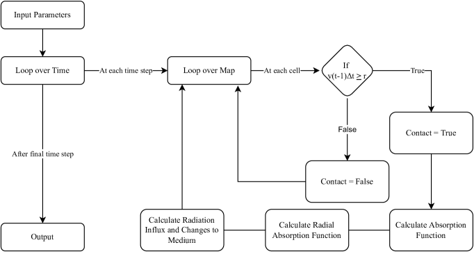
Figure 1: A flow chart showing the basic underlying mechanism of the radiative front model. $r$ is the radial distance to the inner edge of the cell in question, $t$ is the time step coordinate, $\Delta t$ is the real time duration of each time step, and $v$ is the speed of the radiation causing the front, such that the cell in question can be considered to be in contact with the radiation in any timestep for which $v(t-1)\Delta t>r$. In the case of a background which allows for non-trivial transport of the medium through which the front is propagating, transport terms will be included in the cell parameter calculations to represent this. In the event that the radiation is travelling at less than the speed of sound in that medium, an additional series of statements would need to be added within the loop over the map to find which cells are within range of medium transport and recalculate those cell’s parameters even when they are out of range of the radiation.

III Example Application - Ionisation in Astrophysical Media

III.1 Background

The earliest stars were composed almost entirely of hydrogen and helium, and they are known as Population-III stars. [11, 12]. They were large and bright and emitted predominantly ultraviolet radiation. They were also short lived, with lifespans generally not more than a few million years. They are believed to have first come into existence during the transition from what are called the cosmological dark ages, during which the baryonic component of the Universe was primarily composed of neutral hydrogen (HI), to the EoR, during which that HI was predominantly converted into the ionised hydrogen (HII) that composes most of the baryonic matter of the Universe today [13, 14], beginning at a redshift of approximately $z=15$ [15].

An understanding of the ionisation dynamics around individual objects as Population-III stars is essential for high precision studies of the EoR, in particular, those being carried out by the 21cm surveys [16, 17, 18] though there is no precise model able to describe in detail the evolution, spatial extent and morphological structures of the fronts these sources create which determine the tomographic features to be observed in the 21cm spectral lines [19].

When ionising light travels through a medium containing neutral atoms, each photon will have a probability of ionising an atom of

$$\Pi=1-e^{-\tau}\ ,$$ (9)

where

$$\tau=\sigma d$$ (10)

is the optical depth of the path traversed for interaction cross-section $\sigma$ and the column density of the path $d=\rho_{\mathrm{HI}}l$ for HI number density $\rho_{\mathrm{HI}}$ and distance $l$. In the case of neutral hydrogen (HI) being converted to ionised hydrogen (HII), $\sigma=6.3\times 10^{-18}\leavevmode\nobreak\ \mathrm{cm^{-2}}$.

$$\Gamma_{\mathrm{B}}=n_{\mathrm{e}}n_{\mathrm{p}}\alpha\leavevmode\nobreak\ ,$$ (11)

for electron number density $n_{\mathrm{e}}$, proton number density $n_{\mathrm{p}}$, and B-recombination coefficient [20, 21, 22]

$$\alpha\approx\frac{2.6\times 10^{-13}}{(T/10^{4}{\rm K})^{4/5}}$$ (12)

with units of volume per unit time, where $T$ is the average temperature of the medium.

Due to B-recombinations, there will always be a theoretical limit to how large a photoionised bubble can be for a given radiation source. That limit, given under the assumption that the system remains radiating and unchanging except for the interaction of the radiation and the medium for all of time, is given by the Strömgren radius [23]:

$$r_{\mathrm{S}}=\left(\frac{3\phi}{4\pi n_{\mathrm{e}}n_{\mathrm{p}}\alpha}\right)^{\frac{1}{3}}\leavevmode\nobreak\ ,$$ (13)

where $\phi$ is the total flux of photoionising particles being emitted. This can be trivially rearranged to see that it is defined as the radius of a sphere around a radiative object at which the flux of radiation is equal to the number of B-recombinations; assuming that each photon can ionise only one particle, this will of course be the limiting radius of an ionisation bubble. In the event that the ionising particles are able to ionise more than one atom each, this could be corrected by simply multiplying $\phi$ by the number of atoms each particle could ionise.

Of course, Eq. (13) is not an entirely accurate model even for the idealised assumptions we are making; since the flux of particles will decrease with distance from the source, the number density of electrons and protons will also decrease, such that $r_{\mathrm{S}}$ should more realistically be phrased as an integral over spacetime with variable number densities. Since Eq. (13) would generally be calculated under the assumption that within the ionised region the number densities of ionised products equals the initial number density of neutral hydrogen and, if we were to proceed with such a more detailed analogue of the Strömgren radius, we would expect that they would decrease with distance, we would find that such a calculation would yield a slightly higher result. Therefore, we would expect the radius calculated with Eq. (13) to actually be slightly smaller than the maximum radius reached by the ionisation front of a star. Effectively, Eq. (13) assumes a hard cutoff at which complete ionisation gives way to complete neutrality, while failing to take into account the existence of an intermediating front at all.

III.2 Implementation

We wish to model the physics described in Sec. III.1 with the model we described in Sec. II. Specifically, we wish to model the evolution of the ionisation front around a single Population-III star in a neutral background medium during the EoR by treating the star as a source of radiation at the origin of a polar coordinate system and studying the effects of the radiation on the matter in the cell’s that compose the spherical polar map. The speed of the radiation is the speed of light such that cells are considered to be in contact with the source when $r_{i,\theta,\phi}\leq c(t-1)\Delta t$ where $c$ is the speed of light and we are assuming a negligible difference between the speed of light in a vacuum and the speed of sound of the light in the medium.

The absorption function of a given cell is given by its optical depth

$$\tau_{t,i,\theta,\phi}=\sigma\;\!\rho_{\mathrm{HI};t,i,\theta,\phi}l\leavevmode\nobreak\ ,$$ (14)

for cross-section $\sigma$ and cell depth $l=r_{i+1}-r_{i}$. From the definition of $\tau$, we have that $e^{-\tau}$ is the fraction of radiation that transmits through the medium without scattering.

The radial absorption function is then given by a sum over the optical depths of the preceding cells in the same angular bin,

$$s_{t,i,\theta,\phi}=\sum_{j=1}^{i-1}\;\!\tau_{t,j,\theta,\phi}\ .$$ (15)

In order to calculate the flux of radiation reaching each cell at each time step, we must not only account for the division of the star’s overall flux throughout the angular components of the map, but also for the absorption that takes place before they reach a given cell. Thus, the radiation intensity at a given cell will be a function of the overall stellar luminosity $L$, the number of angular components $N_{\theta}$ and $N_{\phi}$, and the radial optical depth $S_{t,i,\theta,\phi}$.

Thus, at a given cell which we label cell $i$, we have that the ionising radiation intensity is given by

$$J_{t,i,\theta,\phi}=\frac{Le^{-s_{t,i,\theta,\phi}}}{N_{\theta}N_{\phi}}\Delta t\leavevmode\nobreak\ .$$ (16)

The ionisation rate within that cell is then given by

$$\Gamma_{t,i,\theta,\phi}=\frac{JN}{h\nu}(1-e^{-\tau_{t,i,\theta,\phi}})\ ,$$ (17)

where $N$ is the number of atoms each photon is capable of ionising, given by $N=\lfloor h\nu/E_{\mathrm{i}}\rfloor$ where $E_{\mathrm{i}}$ is the energy needed to ionise a ground state atom. In the event that multiple types of radiation are emitted, we can generalise Eq. (17) to become a sum over the different wavelengths emitted or, in the event of a continuous distribution of radiation wavelengths, this could be further generalised to

$$\Gamma_{t,i,\theta,\phi}=\int{\rm d}j\ \frac{J_{j}N_{j}}{h\nu_{j}}\;\!\left(1-e^{-\tau_{j,t,i,\theta,\phi}}\right)\ ,$$ (18)

where $N_{j}=\lfloor h\nu_{j}/E_{\mathrm{i}}\rfloor$. However, for this simplified study we content ourselves to treat the star’s radiation as being purely composed of $13.6\mathrm{eV}$ ultraviolet light; given the heavily ultraviolet spectrum of a Population-III star, this is not a particularly inaccurate treatment and will allow accurate results to a level of precision that is satisfactory for the present study.

Given that HI has only one electron, we treat $n_{\mathrm{e}}=n_{\mathrm{p}}=n_{\mathrm{HII}}$, such that Eq. (11) can be implemented as

$$\Gamma_{\mathrm{B};t,i,\theta,\phi}={(n_{\mathrm{HII};t,i,\theta,\phi})}^{2}\;\!\alpha_{t,i,\theta,\phi}\;\!V_{i,\theta,\phi}\;\!\Delta t\ .$$ (19)

As a first approximation, we treat the temperature of all cells as being constant, at $10^{4}\mathrm{K}$. This is an appropriate temperature of such ionised media. Furthermore, we treat the astrophysical medium as being entirely composed of hydrogen, such that at all times we will have $n_{\mathrm{e}}=n_{\mathrm{p}}$ and $N=\lfloor\;\!h\nu/13.6\;\!{\rm eV}\;\!\rfloor$. In a detailed study relevant to 21cm surveys, we would want to use a more detailed analysis with variable temperatures and a medium containing helium, but for the purposes of demonstrating the radiative front model and its application to the evolution of photoionised fronts, these approximations are valid, particularly when one bears in mind that the Strömgren radius given in Eq. (13) assumes a purely hydrogen background and is itself a function of temperature, which we can also set to a constant $10^{4}\leavevmode\nobreak\ \mathrm{K}$.

Thus, at each time step we are altering each cell’s HI and HII count by

$$n_{\mathrm{HI};t,i,\theta,\phi} =n_{\mathrm{HI};t-1,i,\theta,\phi}-\Gamma_{t,i,\theta,\phi}+\Gamma_{\mathrm{B};t,i,\theta,\phi}\leavevmode\nobreak\ ,$$ (20)

$$n_{\mathrm{HII};t,i,\theta,\phi} =n_{\mathrm{HII};t-1,i,\theta,\phi}+\Gamma_{t,i,\theta,\phi}-\Gamma_{\mathrm{B};t,i,\theta,\phi}\leavevmode\nobreak\ ,$$ (21)

in a manner that naturally preserves the overall number of particles per cell, before recalculating the optical depths as

$$\tau_{t+1,i,\theta,\phi} =\sigma\rho_{\mathrm{HI};t,i,\theta,\phi}l\leavevmode\nobreak\ ,$$ (22)

$$s_{t+1,i,\theta,\phi} =\sum_{j=1}^{i-1}\tau_{t+1,j,\theta,\phi}\leavevmode\nobreak\ ,$$ (23)

in preparation for the next time step.

III.3 Application

We demonstrate the model by taking the example of a $100\leavevmode\nobreak\ \mathrm{M_{\odot}}$ Population-III star in a homogeneous background composed entirely of HI with a number density of $\rho_{\mathrm{HI}}=5\times 10^{-6}\;\!(1+z)^{3}\mathrm{\leavevmode\nobreak\ cm^{-3}}$ [24], where the bracketed term accounts for the reduction in density with the expansion of the Universe. Such a star would have a lifespan of approximately $2.7\leavevmode\nobreak\ \mathrm{Myr}$ and would emit $2.4\times 10^{51}\mathrm{\leavevmode\nobreak\ eV\leavevmode\nobreak\ s}^{-1}$ of predominantly ultraviolet radiation [12], which for the sake of simplicity we treat as being purely $13.6\leavevmode\nobreak\ \mathrm{eV}$ light. With these parameters, we generated homogeneous density maps with densities equal to the average densities at $z=15$, $z=10$, and $z=5$.

Before using the model to obtain new results, we would like to confirm that it is consistent with existing ones. In order to do this, we allow the stars to exist for unrealistically long lifespans and compare the maximum radii of their ionised bubbles to the Strömgren radii calculated from Eq. (13). In Fig. 2, we plot the maximum extent of the front against the Strömgren radii calculated from Eq. (13) at the same three redshifts, where the maximum extent of the front is defined in the algorithm as being the inner radius of the cells at which $1-n_{\mathrm{HI};t,i,\theta,\phi}/n_{\mathrm{HI};0,i,\theta,\phi}>0$ and $1-n_{\mathrm{HI};t,i+1,\theta,\phi}/n_{\mathrm{HI};0,i+1,\theta,\phi}=0$. In these cases, we adjusted the run time of the model to account for the respective times it took for the front to reach an equilibrium at the different redshifts, changing the length of each time step accordingly, as well as altering the radius of each cell. In the $z=15$ case, we used cell radii of $2.5\leavevmode\nobreak\ \mathrm{pc}$ and time steps of $450\leavevmode\nobreak\ \mathrm{years}$, in the $z=10$ case we used a cell radius of $5.2\leavevmode\nobreak\ \mathrm{pc}$ and time steps of $1000\leavevmode\nobreak\ \mathrm{years}$, and in the $z=5$ case we used cell radii of $18\leavevmode\nobreak\ \mathrm{pc}$ and time steps of $5000\leavevmode\nobreak\ \mathrm{years}$. Due to the isotropy of the map, we used $N_{\theta}=N_{\phi}=1$ in order to maximise computational efficiency.

We can see that the curves end up slightly exceeding the Strömgren radius, as expected. We also see that in higher densities, ionisation fronts tend to reach this equilibrium position sooner; in the case of $z=5$, for example, it took approximately $500\leavevmode\nobreak\ \mathrm{Myr}$ for the front to stop expanding, while in the case of $z=15$ it too approximately $50\leavevmode\nobreak\ \mathrm{Myr}$. This is in keeping with the notion that, in higher density, regions, the higher rate of B-recombinations will bring about a total radiation absorption in a smaller time frame as well as a smaller volume.

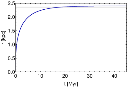
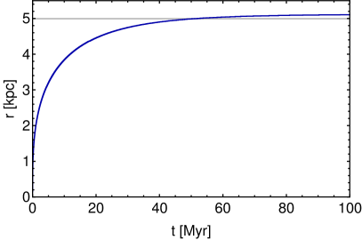
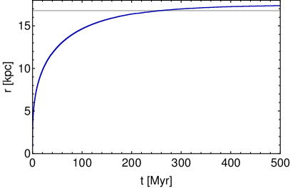
Figure 2: The maximum extent of the ionisation front, defined as being the radius of the cell at which $1-n_{\mathrm{HI},t,i,\theta,\phi}/n_{\mathrm{HI,0},t,i,\theta,\phi}>0$ and $1-n_{\mathrm{HI},t,i+1,\theta,\phi}/n_{\mathrm{HI,0},t,i+1,\theta,\phi}=0$, over periods of time far greater than the realistic lifespan of a Population-III star assuming a constant density as given by the average densities at $z=15$ (top left panel), $z=10$ (top right panel), and $z=5$ (bottom panel), showing that, as expected, the ionisation fronts slightly exceed the Strömgren radii calculated from Eq. (13), plotted alongside the model’s results as grey lines.

Having confirmed that the model is consistent with expected results, we may use it to generate new results by studying the composition of the photoionised region and the front that borders it in more detail. We therefore set the stars to exist for their realistic lifespan of $2.7\leavevmode\nobreak\ \mathrm{Myr}$ and ran the model with time steps of $2000\leavevmode\nobreak\ \mathrm{years}$ and cell radii of, in the case of $z=15$, $17.14\leavevmode\nobreak\ \mathrm{pc}$, in the case of $z=10$, $8.57\leavevmode\nobreak\ \mathrm{pc}$, and in the case of $z=5$, $5\leavevmode\nobreak\ \mathrm{pc}$, once again setting $N_{\theta}=N_{\phi}=1$ for efficiency since we are assuming a homogeneous cosmological background.

Running the model thus, we obtain the results shown in Fig. 3. These figures show the evolution of the angularly symmetric front with time, defined through the ratio $1-n_{\mathrm{HI}}/n_{\mathrm{HI,0}}=n_{\mathrm{HII}}/n_{\mathrm{HII,0}}$, the fraction of the medium which has been ionised. As can clearly be seen, photoionised bubbles in higher density media as are presented by the higher redshift samples evolve more slowly and with a thinner front. Indeed, not only do the higher density samples present smaller bubbles and fronts, but the ratio of the width of the front to the width of the photoionised region is much lower, indicating that the radiation is able to penetrate partially ionised cells much less effectively due to their higher count of HI particles. We also find that the front during the earlier phases of expansion is much thinner than this and only becomes thicker with a more apparent gradient as the ionised bubble becomes larger, which is what one might intuitively expect as the radiation becomes more dispersed and so begins to ionise the media it is in contact with at a lower rate.

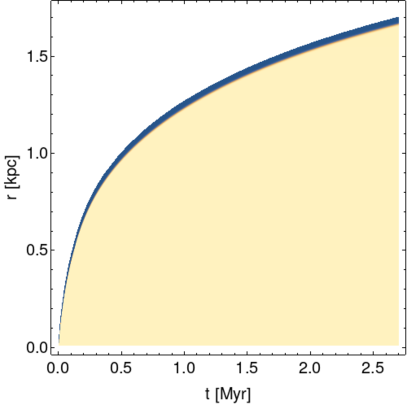
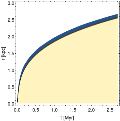
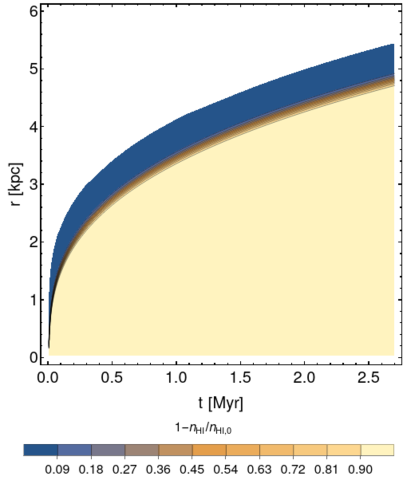
Figure 3: The evolution in time of the photoionisation front created by a Population-III star emitting $2.4\times 10^{51}\mathrm{\leavevmode\nobreak\ eV\leavevmode\nobreak\ s}^{-1}$ of purely $13.6\leavevmode\nobreak\ \mathrm{eV}$ ultraviolet light consistently from its creation to its destruction at an age of $2.7\mathrm{Myr}$ at $z=15$ (top left (panel), $z=15$ (top right panel), and $z=5$ (bottom panel), under the approximation of a constant background density at each redshift. The hydrogen to the outside of the front is almost entirely neutral, that inside it is almost entirely ionised with a small amount of constant recombination preventing full ionisation from ever occurring, and the region within the front is defined as being the region that has a reduced ionised to neutral hydrogen ratio $1-n_{\mathrm{p}}/n_{\mathrm{H}}$ of between $0$ and $1$. As one would expect, the photoionised bubble evolves more quickly and to a larger size in eras with a lower matter density and the front at a given time is wider, as the lower optical depth of the medium allows a greater depth of space to be being ionised simultaneously. Cells in which $n_{\mathrm{HI}}=n_{\mathrm{HI,0}}$ at a given time step are not plotted and therefore make up the region beyond the blue curve of the outer layer of the front.

Taking another example, that of an inhomogeneous background density, once again with a supersonic ionisation front and the same stellar parameters, we define a density map in which the background is primarily defined as being the average density at $z=5$ with a region of overdensity at $\theta=3\pi/2$ which decreases exponentially around that centre until it vanishes at $\theta=0$ and $\theta=\pi$. Allowing the star to live for the unrealistic timeframe examined for the results shown in Fig. 2 and studying again the maximum extent of the front, we find that a slice in time and the homogeneous angular dimension gives a final ionisation front at $2.7\leavevmode\nobreak\ \mathrm{Myr}$ which varies with density, as shown in Fig. 4. This serves to highlight the models ability to study supersonic radiative transport in inhomogeneous media, such as in a region of space containing nebulae and other sources of over- and underdensity.

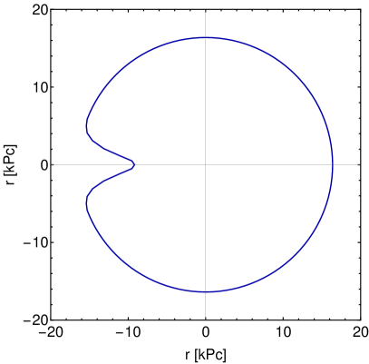
Figure 4: A slice in $\phi$ of the maximum extent of the ionisation front, defined as being the radius of the cell at which $1-n_{\mathrm{HI};t,i,\theta,\phi}/n_{\mathrm{HI,0};t,i,\theta,\phi}>0$ and $1-n_{\mathrm{HI};t,i+1,\theta,\phi}/n_{\mathrm{HI,0};t,i+1,\theta,\phi}=0$, after a period of time of $500\leavevmode\nobreak\ \mathrm{Myr}$ with a density contrast defined at $r\geq 9\leavevmode\nobreak\ \mathrm{kPc}$ around $\theta=3\pi/2$ and exponentially decreasing around that angle before vanishing at $\theta=0$ and $\theta=\pi$.

IV Discussion

We have proposed a new method for modelling the evolution of fronts around radiative objects and have examined the example application of the ionisation bubble around a star in a neutral medium. We have shown that this method agrees with existing methods for estimating basic parameters of the front while providing significantly more information than those methods, allowing us to precisely model its evolution in time as a function of all relevant physical parameters. We propose that this method could find many uses in varied fields, from modelling the effects of ionising radiation as examined here, to modelling chemical photocatalysis, to studying more varied phenomenon such as the propagation of ant expeditions as they explore the territory around their nests. We intend to continue the development of this model and use it for astrophysical applications, specifically using it to study ionising objects during the cosmological epoch of reionisation and how the information this model provides can be applied to upcoming studies of 21cm spectroscopy and we encourage members of other academic groups to apply this method with appropriate modifications and parameters to their own fields.

The current formulation of the Radiative Front Model relies upon a static medium through which the front is propagating; this works for a supersonic front, but would run into issues when describing subsonic fronts as they are much more likely to encounter alterations due to fluid transport caused by the change of state they herald. Furthermore, the model assumes that no radiation is scattered to non-radiative angles.

The subsonic front issue could be corrected for by introducing a set of medium transport equations into the model which allow the particle number to change between cells in a manner that preserves the overall particle number over the set of cells.

The scattering of radiation could be accounted for in one of a number of ways; the simplest would be to incorporate a scalar field into the grid which affects each cell as a function of the conditions of its surrounding cells, effectively modelling the non-radiative scattering by taking an average of its expected effects and applying them directly to each cell. Alternatively, the radiation could be modelled coming out of each cell in which non-radiative scattering is occurring directly before being mapped onto the initial polar coordinate system of cells; however, this method would be significantly more computationally expensive.

Another possible modification which could improve both the precision and computational efficiency of the model would involve dividing each cell into smaller subcells which could be selectively explored depending upon the circumstances; for example, regions well within or well outside the front could be treated as single units, while transitional front cells could be divided up to get a smoother description of the front as it evolves. This could be performed by assigning regions that have been transitioned enough to be considered no longer a part of the front but a part of the altered region with a logical statement and then grouping all cells in contact with each other with that logical statement together as one larger cell, while taking all cells that are in contact with the radiation but are still considered to be a part of the front into smaller cells. However, for the purposes of this paper which was intended to describe and demonstrate our new method, we restricted ourselves to the simpler example of using fixed cell sizes.

We leave it to a future paper to explore these potential extensions of the model in more detail and limit ourselves to the study of entirely radiative, supersonic fronts in this paper.

References

- Sethian [1996] J. A. Sethian, Level Set Methods and Fast MArching Methods (Cambridge University Press, Cambridge, 1996).
- Gibou et al. [2018] F. Gibou, R. Fedkiw, and S. Osher, A review of level-set methods and some recent applications, Journal of Computational Physics 353, 82 (2018).
- Osher [1993] S. Osher, A level set formulation for the solution of the dirichlet problem for hamilton–jacobi equations, SIAM Journal on Mathematical Analysis 24, 1145 (1993), https://doi.org/10.1137/0524066 .
- Osher and Fedkiw [2003] S. Osher and R. Fedkiw, The Level Set Methods and Dynamic Implicit Surfaces (Springer-Verlag, New York, 2003).
- Sethian [1996] J. A. Sethian, A fast marching level set method for monotonically advancing fronts., Proceedings of the National Academy of Sciences 93, 1591 (1996), https://www.pnas.org/doi/pdf/10.1073/pnas.93.4.1591 .
- Sethian [1999] J. A. Sethian, Fast marching methods, SIAM Review 41, 199 (1999).
- Tcheng and Nave [2016] A. Tcheng and J.-C. Nave, A fast-marching algorithm for nonmonotonically evolving fronts, SIAM Journal on Scientific Computing 38, A2307 (2016).
- Goldsworthy [1961] F. A. Goldsworthy, Ionization Fronts in Interstellar Gas and the Expansion of HII Regions, Philosophical Transactions of the Royal Society of London Series A 253, 277 (1961).
- Ducharme et al. [1990] S. Ducharme, J. Hautala, and P. C. Taylor, Photodarkening profiles and kinetics in chalcogenide glasses, Phys. Rev. B 41, 12250 (1990).
- Altay and Wise [2015] G. Altay and J. Wise, Rabacus: A Python Package for Analytic Cosmological Radiative Transfer Calculations, Astron. Comput. 10, 73 (2015), arXiv:1502.02798 [astro-ph.CO] .
- Glover [2005] S. Glover, The Formation Of The First Stars In The Universe, Space Science Review 117, 445 (2005), arXiv:astro-ph/0409737 .
- Wise [2011] J. Wise, First Light, in New Horizons in Astronomy (2011) p. 13.
- Loeb and Barkana [2001] A. Loeb and R. Barkana, The Reionization of the Universe by the first stars and quasars, Ann. Rev. Astron. Astrophys. 39, 19 (2001), arXiv:astro-ph/0010467 .
- Liu and Bromm [2020] B. Liu and V. Bromm, When did Population III star formation end?, MNRAS 497, 2839 (2020), arXiv:2006.15260 [astro-ph.GA] .
- Koopmans et al. [2015] L. V. E. Koopmans et al., The Cosmic Dawn and Epoch of Reionization with the Square Kilometre Array, PoS AASKA14, 001 (2015), arXiv:1505.07568 [astro-ph.CO] .
- Di Matteo et al. [2004] T. Di Matteo, B. Ciardi, and F. Miniati, The 21 Centimeter emission from the reionization epoch: Extended and point source foregrounds, MNRAS 355, 1053 (2004), arXiv:astro-ph/0402322 .
- Pritchard and Loeb [2012] J. R. Pritchard and A. Loeb, 21-cm cosmology in the 21st century, Rep. Prog. Phys. 75, 086901 (2012), arXiv:1109.6012 .
- Smoot, George F. and Debono, Ivan [2017] Smoot, George F. and Debono, Ivan, 21 cm intensity mapping with the five hundred metre aperture spherical telescope, A&A 597, A136 (2017).
- Mirocha et al. [2018] J. Mirocha, R. H. Mebane, S. R. Furlanetto, K. Singal, and D. Trinh, Unique signatures of Population III stars in the global 21-cm signal, MNRAS 478, 5591 (2018), arXiv:1710.02530 [astro-ph.GA] .
- Osterbrock and Ferland [2006] D. E. Osterbrock and G. J. Ferland, Astrophysics of gaseous nebulae and active galactic nuclei (University Science Book, Sausalito, CA, 2006).
- Seaton [1959] M. J. Seaton, The solution of capture-cascade equations for hydrogen, MNRAS 119 (1959).
- Pengelly [1964] R. M. Pengelly, Recombination spectra, I, MNRAS 127 (1964).
- Strömgren [1939] B. Strömgren, The Physical State of Interstellar Hydrogen., Astrophys. J. 89, 526 (1939).
- Crighton et al. [2015] N. H. M. Crighton et al., The neutral hydrogen cosmological mass density at z = 5, MNRAS 452, 217 (2015), arXiv:1506.02037 [astro-ph.CO] .