Implementation of advanced Riemann solvers in a neutrino-radiation magnetohydrodynamics code in numerical relativity and its application to a binary neutron star merger
Abstract
We implement advanced Riemann solvers HLLC and HLLD Mignone and Bodo (2005); Mignone et al. (2009) together with an advanced constrained transport scheme Gardiner and Stone (2008) in a numerical-relativity neutrino-radiation magnetohydrodynamics code. We validate our implementation by performing a series of one- and multi-dimensional test problems for relativistic hydrodynamics and magnetohydrodynamics in both Minkowski spacetime and a static black hole spacetime. We find that the numerical solutions with the advanced Riemann solvers are more accurate than those with the HLLE solver Del Zanna et al. (2003), which was originally implemented in our code. As an application to numerical relativity, we simulate an asymmetric binary neutron star merger leading to a short-lived massive neutron star both with and without magnetic fields. We find that the lifetime of the rotating massive neutron star formed after the merger and also the amount of the tidally-driven dynamical ejecta are overestimated when we employ the diffusive HLLE solver. We also find that the magnetorotational instability is less resolved when we employ the HLLE solver because of the solver’s large numerical diffusivity. This causes a spurious enhancement both of magnetic winding resulting from large scale poloidal magnetic fields, and also of the energy of the outflow induced by magnetic pressure.
I Introduction
The first direct detection of gravitational waves from a binary neutron star merger (GW170817) and its electromagnetic counterparts (AT 2017gfo/SGRB 170817A) heralded the beginning of multimessenger astronomy including gravitational waves Abbott et al. (2017a, b). In this event, the tidal deformability of the neutron star binary was measured for the first time and found to be in the interval , with an accurate measurement of the total mass of the binary yielding Abbott et al. (2017a, 2019, 2018); De et al. (2018) 111The precise value of depends on the details of the analysis.. Any viable neutron star matter equations of state must satisfy this observational constraint on tidal deformability. In this event it was also shown that the binary neutron star merger drives a short gamma-ray burst Goldstein et al. (2017); Abbott et al. (2017b); Savchenko et al. (2017); Mooley et al. (2018), thus providing the first ‘smoking gun’ for supporting the hypothesis that binary mergers can be the central engine of short gamma-ray bursts Paczynski (1986); Goodman (1986); Eichler et al. (1989); Narayan et al. (1992). Finally, this event indicated that neutron-rich matter is likely to be ejected during the merger and heavy elements are synthesized within these ejecta by means of the rapid neutron capture process on nuclei (the -process) Metzger et al. (2010); Lattimer and Schramm (1974); Eichler et al. (1989); Wanajo et al. (2014). It had been predicted that the -process nucleosynthesis subsequently causes so-called kilonova emission via the radioactive decay of unstable -process elements Tanaka and Hotokezaka (2013); Barnes and Kasen (2013), and a kilonova was indeed observed after the merger in the near infrared, optical, and ultraviolet bands Arcavi et al. (2017); Chornock et al. (2017); Coulter et al. (2017); Cowperthwaite et al. (2017); Drout et al. (2017); Kasen et al. (2017); Kasliwal et al. (2017); Kilpatrick et al. (2017); McCully et al. (2017); Nicholl et al. (2017); Shappee et al. (2017); Smartt et al. (2017); Soares-Santos et al. (2017); Tanaka et al. (2017); Tanvir et al. (2017).
References Abbott et al. (2020, 2021) reported the detection of a second binary neutron star merger event (GW190425) and measured a total binary mass of , which is much larger than the total mass measured in binary pulsars observed in our Galaxy Farrow et al. (2019). The merger dynamics, mass ejection process, and resultant electromagnetic emission due to -process nucleosynthesis could be different from those in GW170817 and AT 2017gfo Kyutoku et al. (2020); Dudi et al. (2021). Although an electromagnetic counterpart was not observed in GW190425, either due to poor sky localization or due to intrinsically dimmer emission Hosseinzadeh et al. (2019); Coughlin et al. (2019, 2020), the existence of a massive binary neutron star suggests that the binary neutron star merger and associated mass ejection process could have a diversity of mechanisms. The new observation run O4 is planned to commence at the end of 2022 O4- , and could lead to the observation of binary neutron star mergers and associated electromagnetic counterparts that are qualitatively different from those observed in GW170817. This motivates building binary neutron star merger models based on reliable numerical relativity simulations for predicting and interpreting gravitational wave events in preparation for the upcoming observational run Shibata et al. (2017).
Recent axisymmetric neutrino-radiation viscous-hydrodynamics simulations of binary neutron star merger remnants in numerical relativity suggest that the amount of post-merger ejecta launched from the merger remnant due to viscous effects (which were facilitated in these simulations by an effective ‘alpha’ viscosity parameter) can be larger than the dynamical ejecta launched during the merger itself Fujibayashi et al. (2018, 2020a, 2020b, 2020c); Shibata et al. (2017). The timescale of the post-merger mass ejection is second, and depends on the value of the viscosity parameter. Plausible values of the viscosity parameter are inferred from three-dimensional magnetohydrodynamics simulations of the binary neutron star merger remnant in which angular momentum transport is facilitated in a self-consistent manner by the magnetorotational instability Kiuchi et al. (2018) (see also Refs. Christie et al. (2019); Fernández et al. (2019) for magnetohydrodynamics simulations of a massive torus in a stationary black hole spacetime). The electron fraction of the post-merger ejecta and the resultant -process nucleosynthesis also depends on this viscosity parameter Fujibayashi et al. (2020b, a, c), although the electron fraction of the post-merger ejecta is appreciably larger than that of the dynamical ejecta.
Furthermore, very recently we performed neutrino-radiation magnetohydrodynamics simulations of black hole-neutron star mergers in numerical relativity Hayashi et al. (2021). We found post-merger mass ejection due to magnetorotational instability-driven turbulence and the launch of a Poynting flux-dominated outflow. The post-merger mass ejection and the Poynting-flux dominated outflow sets in at several ms after the merger and lasts for – seconds after the merger. These timescales are determined by the strength of the effective viscosity associated with both magnetorotational-instability turbulence and neutrino cooling Hayashi et al. (2021).
All these recent studies show that for modeling future gravitational wave events it is necessary to perform self-consistent (i.e. in which turbulence is sustained by the magnetorotational instability) three-dimensional neutrino-radiation magnetohydrodynamics simulations of binary neutron star mergers in general relativity for the durations of second. In particular, it is crucial to reproduce a magneto-turbulent state driven by the magnetorotational instability inside the merger remnant because the resultant effective turbulent viscosity transports angular momentum outwards and heats up the matter via viscous heating Balbus and Hawley (1998).
Finite volume methods are a popular combination of numerical schemes for simulations of astrophysical fluid dynamics due to their inherent conservation properties and ability to capture sharp discontinuities in the flow such as shocks Toro (2013). Central to these schemes is the solution of the so-called Riemann problem in which one considers two constant states separated by a discontinuity. The solution consists of three waves in hydrodynamics and seven waves in magnetohydrodynamics. As exact Riemann solvers are computationally expensive Giacomazzo and Rezzolla (2006), approximate Riemann solvers are often used. One such family of approximate Riemann solvers is the HLL-based Riemann solvers, in which only a subset of the full seven waves in the Riemann fan are considered. The HLL(E) solver, for example, takes into account only shocks/rarefactions and omits the contact discontinuity Harten et al. (1983).
At present, the Riemann solver and constrained transport scheme implemented in existing numerical relativity magnetohydrodynamics codes, e.g. Hayashi et al. (2021); Radice et al. (2021); Bernuzzi and Dietrich (2016); Most et al. (2019); Mösta et al. (2014); Etienne et al. (2015); Viganò et al. (2020); Cipolletta et al. (2021); Foucart et al. (2021), are based on the HLLE solver Kurganov and Tadmor (2000); Harten et al. (1983); Del Zanna et al. (2003). (An exception is the SpECTRE Deppe et al. (2021) code, which is based on the discontinuous Galerkin method.) This Riemann solver is known to be very diffusive Toro et al. (1994); Mignone et al. (2009); Held and Latter (2018). The numerical diffusion inherent in the Riemann solver adversely affects the accuracy of the numerical solution, in particular for long-term simulations of compact object mergers of second. Although Refs. Bernuzzi and Dietrich (2016); Most et al. (2019); Radice et al. (2014) reported the implementation of fourth-order accurate Riemann solvers in their numerical relativity codes, these solvers are based on the finite difference method. Therefore, it is unclear how accurate these finite difference-based Riemann solvers are for the problem of astrophysical turbulence.
This paper reports a new implementation of advanced Riemann solvers in our neutrino-radiation magnetohydrodynamics numerical relativity code Kiuchi et al. (2012); Sekiguchi et al. (2012) based on the finite volume method. We implement the HLLC solver for relativistic hydrodynamics, which restores the contact discontinuity Mignone and Bodo (2005), and the HLLD solver for relativistic magnetohydrodynamics, which takes into account five of the seven waves in the Riemann fan Mignone et al. (2009). Both these Riemann solves are known to be less diffusive than the HLLE solver Del Zanna et al. (2003). In addition, the constrained transport scheme in Ref. Gardiner and Stone (2008), which relies on the solution given by a Riemann solver, significantly suppresses numerical diffusion compared to the HLLE-constrained transport scheme proposed in Ref. Del Zanna et al. (2003) (see Ref. Mignone and Del Zanna (2021) for a detailed comparison of different implementations of the constrained transport scheme). Thus, in addition to implementing the advanced Riemann solvers, HLLC and HLLD, we also implement the novel constrained transport scheme of Ref. Gardiner and Stone (2008) in our code.
This paper is organized as follows. Section II summarizes the equations of motion for general relativistic neutrino-radiation magnetohydrodynamics. Section III is devoted to the numerical algorithm for general relativistic magnetohydrodynamics: the finite volume method, the constrained transport method (for enforcing divergence-free condition of the magnetic field), the tetrad transformation (which enables us to use Riemann solvers designed for special relativistic flows in full general relativity), the implementation of the HLLC solver Mignone and Bodo (2005), that of the HLLD solver Mignone et al. (2009), and the electric field evaluation (which is used by the constrained transport algorithm) Gardiner and Stone (2008). In Sec. IV, we validate our implementation of the new Riemann solvers by performing one- and multi-dimensional test problems both in Minkowski spacetime and in curved, but static, spacetime in both relativistic hydrodynamics and magnetohydrodynamics. Finally, in Sec. V we apply our new solvers in general relativity to a dynamical spacetime. We first present the results of binary neutron star merger simulations in the absence of magnetic fields (which are run up to – ms after the formation of the black hole), and subsequently the evolution of the merger remnant with a magnetic field. Section VI summarizes our results. Throughout this paper, we use geometrical units in which . Greek and Latin indices without hats denote the spacetime and purely spatial components, respectively. Those with hats indicate tetrad components.
II Governing equations for general relativistic neutrino-radiation magnetohydrodynamics
In this section, we briefly summarize the set of basic equations of general relativistic neutrino-radiation magnetohydrodynamics using the 3+1 formalism. The reader can find a more comprehensive derivation of these equations in, e.g., Ref. Shibata (2016).
We begin by introducing a unit vector normal to a spatial hypersurface of constant coordinate time, ,
| (1) |
where and are the lapse function and shift vector, respectively. With this vector, the four dimensional metric can be decomposed into
| (4) |
where is the three-dimensional spatial metric.
The stress-energy-momentum tensor for ideal magnetohydrodynamics and for a free-streaming neutrino-radiation field are, respectively, given by
| (5) |
where , , , , , , and are, respectively, the rest-mass density, pressure, four-velocity, magnetic field (measured in the fluid rest frame), radiation energy density, radiation momentum, and radiation stress-energy-momentum tensor of the neutrino species in the Eulerian frame. denotes the relativistic specific enthalpy with the specific internal energy. We consider the electron neutrino , electron antineutrino , and the total of and neutrinos and antineutrinos collectively denoted by Sekiguchi et al. (2012); Shibata (2016). Note that we assume that the stress-energy-momentum tensor of the neutrino-radiation field is split into a trapped component and a free-streaming component. The stress-energy-momentum tensor of the trapped neutrinos is then absorbed into that for the ideal magnetohydrodynamics fluid because trapped neutrinos are strongly coupled to the fluid Sekiguchi et al. (2012); Shibata (2016).
The conserved mass density, total momentum density, and total energy density of an electrically conducting fluid are defined by
| (6) | ||||
| (7) | ||||
| (8) |
where is the Lorentz factor measured by an Eulerian observer and is the magnetic field measured in the Eulerian frame and satisfies (i.e., ). The relation between and is given by
| (9) |
and thus,
| (10) |
where .
The equations of motion of ideal magnetohydrodynamics and of the free-streaming neutrino-radiation field are derived from the conservation of the stress-energy-momentum tensor, the continuity equations for rest-mass density, electron fraction, electron neutrino fraction, electron antineutrino fraction, and heavy neutrino fraction, and the Maxwell equations. These conservation laws are written as
| (11) | |||
| (12) | |||
| (13) | |||
| (14) | |||
| (15) |
where and denotes electrons, electron neutrinos, electron antineutrinos, and heavy neutrinos, respectively. and denote the fractions with respect to the baryon and the source term for the number of the species , respectively. is an interaction term between the fluid and free-streaming neutrino-radiation field of the neutrino species in the framework of a general relativistic neutrino leakage scheme Sekiguchi et al. (2012); Sekiguchi (2010). Here is the Hodge dual of the Faraday tensor, which is given by in ideal magnetohydrodynamics.
Equations (11), (13), and (15) can be written in conservative form as
| (16) | |||
| (17) |
where the flow quantities are given by the state vector with . The corresponding fluxes are given by
and the source terms are
| (22) |
where , , and the spatial components of the stress-energy-momentum tensor are given by
| (23) | |||
| (24) |
We also introduce the conformal metric and the trace-free conformal extrinsic curvature , where and are the conformal factor and the extrinsic curvature, respectively. The explicit forms for and and for the equation of motion of the free-streaming neutrino-radiation field can be found in Refs. Fujibayashi et al. (2017); Shibata (2016). The high resolution shock capturing scheme for the neutrino-radiation field Eq. (12) is the same as that in Ref. Shibata et al. (2011).
III Numerical algorithm
In this section, we describe the numerical algorithms which we implemented in our code. In Sec. III.1 we present the finite volume algorithm and discretization scheme, and in Sec. III.2 we discuss the transformation to Minkowski spacetime used to implement the HLLC and HLLD solvers in general relativity. The implementation of the HLLC and HLLD solvers themselves is presented in Sec. III.3 and III.4, respectively. Finally, the evaluation of the electric field used by the constrained transport algorithm is discussed in Sec. III.5.
III.1 Finite volume method
III.1.1 Fluid and magnetic field at cell center
Let be a region of a given four-dimensional manifold , bounded by a closed three-dimensional surface , where denotes the surface of a four-dimensional parallelepiped composed of two spacelike surfaces and three sets of two timelike surfaces that connect the two temporal slices Font (2003). The timelike surface, e.g., , may also be regarded as a time series of constant- surfaces, . We integrate Eq. (16) over the domain of :
| (25) |
where .
Using Gauss’s theorem, this equation can be integrated to give
| (26) |
where
| (27) | |||
| (28) |
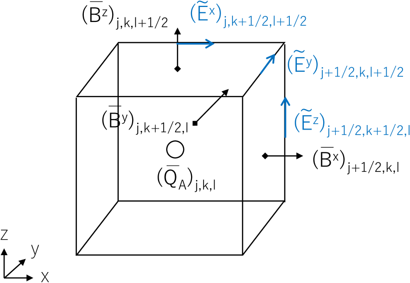
are, respectively, the three-dimensional proper volume-averaged conserved quantities and the proper volume. Let us now define a cell consisting of (see Fig. 1). We next consider a numerical flux, which approximates a time-averaged flux at the cell interface and depends on the solution of the Riemann problem at the interface. For example, in the -direction the flux across the right-hand interface is given by
| (29) |
where . With this numerical flux, Eq. (26) can be discretized as
| (30) |
where
| (31) | |||
| (32) | |||
| (33) |
We also assume that the determinant of the spatial metric does not change significantly during the time step. If we introduce the volume- or surface area-averaged determinant of the spatial metric, denoted by , this equation is reduced to
| (34) |
where
| (35) | |||
| (36) | |||
| (37) | |||
| (38) |
and
| (39) |
III.1.2 Magnetic fields at cell surface
To ensure that the divergence-free condition (17) is maintained, we employ the constrained transport method introduced by Evans and Hawley Evans and Hawley (1988). In this method, the magnetic-field components are defined at the cell surfaces, and the electric field components are defined at the cell edges (see Fig. 1).
We then integrate Eq. (16) for on . For example, through the surface , we have
| (40) |
where , is the three-dimensional Levi-Civita tensor, and . Using Stokes’ theorem, this equation is integrated to give
| (41) |
where
is the surface-averaged magnetic field. Similarly, through the surfaces and , respectively, we have
| (42) | |||
| (43) |
where
We next consider a cell surface consisting of , , and a numerical flux which approximates a time-averaged electric field at the cell edge, given by
| (44) | |||
| (45) | |||
| (46) |
With these averaged electric fields, Eqs. (III.1.2)–(43) are discretized as
| (47) | |||
| (48) | |||
| (49) |
where
| (50) | |||
| (51) | |||
| (52) |
If we introduce a line-averaged determinant of the spatial metric by
| (53) |
then, together with the surface area-averaged spatial metric given by Eqs. (36)–(38), Eqs. (47)–(49) are reduced to
| (54) | |||
| (55) | |||
| (56) |
The magnetic-field distribution inside the cell is reconstructed from the magnetic fields at the cell surface. Practically, we reconstruct the magnetic field at the cell center in Eq. (34) by
| (57) | |||
| (58) | |||
| (59) |
III.2 Tetrad frame
To evaluate the numerical fluxes through cell interfaces (e.g. Eq. (29)), we implement HLL-type Riemann solvers Mignone and Bodo (2005); Mignone et al. (2009). Because these Riemann solvers are designed to solve a Riemann problem in Minkowski spacetime (except for the HLLE solver, which we have implemented directly in curved spacetime, see, e.g., Ref. Shibata and Sekiguchi (2005)), it is necessary to transform all the equations into a tetrad frame in order to apply these methods to a general relativistic framework.
Following Ref. White et al. (2016), we define a tetrad basis in the -direction, for example, by
| (60) | |||
| (61) | |||
| (62) | |||
| (63) |
where
| (64) | |||
| (65) | |||
| (66) |
With this basis, we can perform a transformation from the Eulerian frame to the tetrad frame by
| (67) | |||
| (68) |
where and denote a covariant vector and tensor, respectively, in the Eulerian frame. The covariant components of the tetrad basis are
| (69) | ||||
| (70) | ||||
| (71) | ||||
| (72) |
With this basis, we can then perform the transformation from the tetrad frame to the Eulerian frame by
| (73) | |||
| (74) |
With this tetrad basis the procedure to obtain the numerical flux is as follows: first, we calculate the tetrad component of , and by
| (75) | |||
| (76) | |||
| (77) |
Second, we solve a Riemann problem in the locally Minkowski spacetime to obtain the numerical flux and the conserved quantities at the cell interface (see the next section for more detail on the Riemann problem). Finally, we transform back to the Eulerian frame from the tetrad frame by
| (78) | |||
| (79) | |||
| (80) | |||
| (81) | |||
| (82) | |||
| (83) | |||
| (84) | |||
| (85) |
where are contracted with , respectively, in the second term of the right-hand side of Eqs. (79) and (80). Note that, from now on, we do not distinguish the upper- and lower-spatial tetrad components, e.g., . These numerical fluxes are used to update the conserved quantities in Eq. (34). An interface velocity is calculated by White et al. (2016)
| (86) |
This velocity is used to calculate a numerical flux at the interface (see Eqs. (103) and (137) in the next section). The tetrad basis and numerical fluxes in the - and -directions are summarized in Appendix A.
III.3 HLLC solver for relativistic hydrodynamics
In the absence of electromagnetic fields, Eq. (34) with are reduced to those of relativistic hydrodynamics. In this case, one choice for the Riemann solver is the HLLC solver proposed in Ref. Mignone and Bodo (2005). We calculate the HLLC flux in the tetrad frame by solving the source-free one-dimensional conservation law:
| (87) | |||
| (91) | |||
| (95) |
where . Given an initial condition described by
| (98) |
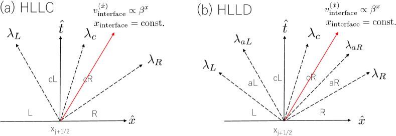
for , three characteristic speeds and therefore four states will appear in the Riemann fan (see Fig. 2). In the HLLC solver, one needs to find the pressure in the intermediate states (the and states) which satisfies a jump condition. Then, the numerical flux is calculated by (see the left panel of Fig. 2)
| (103) |
where
| (104) | |||
| (105) |
and is the characteristic speed of the left/right-going nonlinear wave. Equation (105) is obtained from the jump condition and is the characteristic speed of the contact discontinuity. By imposing continuity of the pressure across the contact discontinuity, one finds a quadratic equation for Mignone and Bodo (2005):
| (106) |
where , , , and denote conserved quantities and fluxes in the HLL state:
| (107) | |||
| (108) | |||
| (109) | |||
| (110) |
Once we obtain the speed of the contact discontinuity , the pressure in the intermediate state is determined by
| (111) |
Then the conserved quantities in the and states are given by
| (112) | |||
| (113) | |||
| (114) |
where the subscripts and on the left-hand side of the equations correspond to and on the right-hand side, respectively. These quantities can be used to evaluate the flux in the state (105) and the flux in the Eulerian frame (see, e.g., Eq. (78)).
For the left and right characteristic speeds , we apply Davis’s estimate Mignone and Bodo (2005):
| (115) | |||
| (116) |
and
| (117) |
where
| (118) | |||
| (119) |
The equivalent expressions in the - and -directions are given by permutation of the indices , and .
III.4 HLLD solver for relativistic magnetohydrodynamics
In the presence of an electromagnetic field, one choice for the Riemann solver is the HLLD solver proposed in Ref. Mignone et al. (2009). For this case, we calculate the HLLD flux, in the tetrad frame by solving the one-dimensional conservation law:
| (120) |
where
| (125) | |||
| (130) |
Here, has seven components (), and is the total pressure (gas plus magnetic). Note that the equation for is simply , and thus, is constant for the Riemann problem of the -direction. Together with the initial condition given by Eq. (98) for the relevant components, the full magnetohydrodynamics Riemann fan consists of seven waves separating eight states Font (2003). In the HLLD solver two of these seven waves (the slow magnetosonic waves) are neglected. As a result, the Riemann fan with the HLLD solver consists of five waves separating six states (see Fig. 2). In the HLLD solver, we need to find the total pressure which satisfies a jump condition across the five waves. The numerical flux is then given by (see the right-hand panel of Fig. 2)
| (137) |
where
| (138) | ||||
| (139) | ||||
| (140) |
The latter two fluxes are obtained from the jump condition.
In the following subsections, we present specific quantities employed by the HLLD solver: the characteristic speeds of the five waves, and the six states.
III.4.1 Characteristic speeds
III.4.2 L/R state
Given left- and right-state quantities, we first calculate the following quantities which should be preserved when one crosses the fast waves:
| (147) | |||
| (148) | |||
| (149) | |||
| (150) |
where for , respectively, in Eq. (148). Also for , respectively, in Eq. (150). For the above quantities, we employ the characteristic speed defined by
| (151) |
III.4.3 aL/aR state
Given an initial guess for the unknown total pressure (which should be constant inside the Riemann fan), the three velocities in the and states are given by
| (152) | |||
| (153) | |||
| (154) |
where
| (155) | |||
| (156) | |||
| (157) | |||
| (158) | |||
| (159) |
Note that and on the left-hand side of Eqs. (152)–(154) correspond to and for , , , and on the right-hand side of the same equations, respectively. With these velocity components, the magnetic field is calculated from the jump condition by
| (160) |
for . The total enthalpy density is calculated by
| (161) |
The conserved quantities necessary for the numerical flux in Eq. (139) and in the Eulerian frame (see Eqs. (78)–(85)) are calculated by
| (162) | |||
| (163) | |||
| (164) |
III.4.4 cL/cR state
Following Ref. Mignone et al. (2009), we first define
| (165) | |||
| (166) |
where the plus (minus) sign corresponds to the right (left) state. We then define by
| (167) |
Here is nothing other than the Alfvén wave speed in the -direction. From the jump condition one can find that , , , and do not change across the Alfvén waves. Therefore, , , and the total enthalpy density are calculated by
| (168) | |||
| (169) | |||
| (170) |
where and on the left-hand side of the equations correspond to and on the right-hand side of the same equations, respectively.
The magnetic field and the three velocity in the and states are calculated by
| (171) | |||
| (172) |
and the characteristic speed is
| (173) |
We impose the continuity condition on the normal velocity across the contact discontinuity, i.e., , by
| (174) | |||
| (175) |
where . This equation gives an improved guess of the total pressure in the next iteration step. Then we go back to Eq. (152) and repeat the same procedure until it converges with sufficient accuracy. In practice, we employ the Newton-Raphson method to solve Eq. (174).
The conserved quantities necessary for the numerical flux in Eq. (140) and in the Eulerian frame (see Eqs. (78)–(85)) are
| (176) | |||
| (177) | |||
| (178) |
The equivalent expressions in the - and -directions are given by permutation of the indices , and .
III.5 Electric-field evaluation
The constrained transport method used to enforce the divergence-free condition on the magnetic field requires us to evaluate the electric field defined at the cell edges. Gardiner and Stone Gardiner and Stone (2008) proposed a method for evaluating the electric-field by utilizing the numerical fluxes which are obtained by the Riemann solver. In their method, for example, the -component of the electric field is evaluated by
| (179) |
where
Here and are identical to the fluxes and in Eqs. (78) and (III.2), which are given by the Riemann solver in the -direction. Similarly, and are given by the Riemann solver in the -direction. is calculated from the quantities defined at the cell center, i.e., Eqs. (57)–(59) and the three velocity. Therefore, the accuracy of this constrained transport scheme depends on the accuracy of an employed Riemann solver. Equivalent expressions for the - and -components of the electric field are given by permutation of the indices and . These electric fields are used to update the magnetic field in Eqs. (54)–(56).
| Test problem | State | CFL | ||||||||||
|---|---|---|---|---|---|---|---|---|---|---|---|---|
| Problem HD1 | L | 4/3 | 1 | 0.9 | 0 | 0 | 1 | – | – | – | 0.4 | 0.8 |
| R | 1 | 0 | 0 | 0 | 10 | – | – | – | ||||
| Problem HD2 | L | 5/3 | 1 | 0 | 0 | 10 | – | – | – | 0.4 | 0.8 | |
| R | 10 | 0.5 | 0 | 0 | 20 | – | – | – | ||||
| Problem HD3 | L | 5/3 | 10 | 0 | 0 | 0 | 40 | – | – | – | 0.4 | 0.8 |
| R | 1 | 0 | 0 | 0 | 3 | – | – | – | ||||
| Problem HD4 | L | 5/3 | 1 | 0 | 0 | 0 | – | – | – | 0.4 | 0.8 | |
| T | 1 | 0 | 0 | 0 | – | – | – | 0.4 | 0.8 | |||
| Problem MHD1 | L | 5/3 | 10 | 0 | 0.7 | 0.2 | 1 | 5 | 1 | 0.5 | 1 | 0.8 |
| R | 1 | 0 | 0.7 | 0.2 | 1 | 5 | 1 | 0.5 | ||||
| Problem MHD2 | L | 5/3 | 1 | 0.4 | 0.5 | 1 | 2.4 | 1 | 1 | 0.8 | ||
| R | 1 | 0.377347 | 0.424190 | 1 | 2.4 | |||||||
| Problem MHD3 | L | 2 | 1 | 0 | 0 | 0 | 1 | 0.5 | 1 | 0 | 0.4 | 0.8 |
| R | 0.125 | 0 | 0 | 0 | 0.1 | 0.5 | 0 | |||||
| Problem MHD4 | L | 5/3 | 1.08 | 0.4 | 0.3 | 0.2 | 0.95 | 2 | 0.3 | 0.3 | 0.55 | 0.8 |
| R | 1 | 0.2 | 1 | 2 | ||||||||
| Problem MHD5 | L | 5/3 | 1 | 0.999 | 0 | 0 | 0.1 | 10 | 7 | 7 | 0.4 | 0.8 |
| R | 1 | 0 | 0 | 0.1 | 10 | |||||||
| Problem MHD6 | L | 5/3 | 1 | 0 | 0.3 | 0.4 | 5 | 1 | 6 | 2 | 0.5 | 0.8 |
| R | 0.9 | 0 | 0 | 0 | 5.3 | 1 | 5 | 2 |
In the rest of this paper, we refer to this particular algorithm for evaluating the electric field as CT_GS. On the other hand, the electric-field evaluation algorithm which was originally implemented in our code, and which is based on HLLE Del Zanna et al. (2003); Shibata and Sekiguchi (2005), is referred to as CT_HLLE Shibata and Sekiguchi (2005). For the base Riemann solver, we use either HLLC, HLLD, or HLLE. Here the last one is the base Riemann solver which was originally implemented in our code Shibata and Sekiguchi (2005). In the hydrodynamics test simulations shown in the next section, we refer to the particular combination of numerical schemes used in a particular test problem in terms of the base solver, only. In the magnetohydrodynamics test simulations, we describe a simulation both in terms of the base Riemann solver and in terms of the algorithm used for the evaluation of the electric-field. For example, HLLD-CT_GS means that the (base) Riemann solver is HLLD and the electric-field evaluation is CT_GS.
IV Validation of the HLLC and HLLD solvers
In this section, we introduce various problems designed to test the implementation of the advanced Riemann solvers and constrained transport algorithm discussed in the previous section. We start with a common suite of one-dimensional special relativistic shock-tube problems in both hydrodynamics and magnetohydrodynamics (see Sec. IV.1). Next, in Sec. IV.2, we turn our attention to multi-dimensional hydrodynamics and magnetohydrodynamics test problems in special relativity (specifically, we consider a two-dimensional hydrodynamical shock, a cylindrical hydrodynamical blast wave, a magnetohydrodynamical current sheet, and the Kelvin-Helmholtz instability in magnetohydrodynamics). In Sec. IV.3 we consider Bondi flow onto a black hole (in both hydrodynamics and magnetohydrodynamics) as a test problem in general relativity with a static spacetime.
For all the test problems we assume a -law equation of state given by
| (180) |
We also employ a cell-centered grid structure in which the -coordinate 222 In Ref. Kiuchi et al. (2012), we employed a vertex-centered grid structure. We updated the interpolation scheme of the metric and fluid at the refinement boundary for cell-centered grid structure for a simulation in a dynamical spacetime. is given by
| (181) |
with and grid spacing (and likewise for the - and -components). As a time integrator, we employ the fourth-order Runge-Kutta method (RK4) in all our test simulations. For reconstruction of the solution at cell-interfaces, we employ either 1st-order reconstruction or 3rd-order piecewise parabolic method (PPM) (Shibata and Sekiguchi, 2005; Colella and Woodward, 1984). For the PPM reconstruction, we employ the min-mod limiter function with a compression parameter which is generally set to Shibata and Sekiguchi (2005), though in some cases we employ different values of .
IV.1 Special relativistic one-dimensional problems
First, we consider special relativistic problems in one spatial dimension. With this setup, the tetrad basis in Sec. III.2 is reduced to a coordinate vector in Minkowski spacetime. Thus, the setup is suitable for validating the Riemann solvers described in Sec. III.3 and III.4. We assume Minkowski metric, and thus turn off the solver for Einstein’s equations in the code. The initial conditions for all the one-dimensional test problems are summarized in Table 1. We note that the test suite employed in this paper is the same as that presented in Refs. Mignone et al. (2009); Mattia and Mignone (2021).
IV.1.1 Hydrodynamics: one-dimensional shock tubes
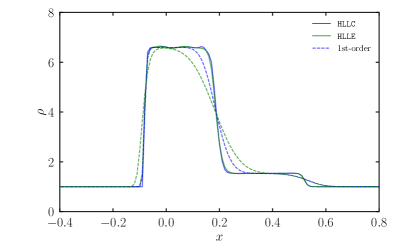
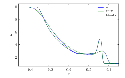
The first special relativistic hydrodynamics test (HD1) is the computation of a contact discontinuity. For this we prepare a simulation domain of with and . We integrate the numerical solution up to . In the left panel of Fig. 3 we plot the rest-mass density profile at the end of the simulation. In this problem, left- and right-propagating shock waves appear from the initial discontinuity, with a contact discontinuity sandwiched between them. The blue and green curves denote the numerical solution with the HLLC and HLLE solvers, respectively. The solid and dashed curves denote the simulation results with 3rd-order PPM reconstruction and 1st-order reconstruction, respectively. First, we consider the results obtained with 1st-order reconstruction (dashed curves). With the HLLC solver, the contact discontinuity located at is more sharply captured than with the HLLE solver. This behavior is expected since the HLLC solver explicitly restores the contact wave inside the Riemann fan. When we employ 3rd-order reconstruction, however, we find that there is no qualitative difference between the two solvers. This suggests that the weak point of a particular solver may be alleviated by using a high enough resolution.
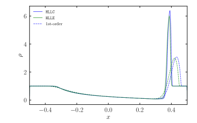
The right panel of Fig. 3 shows the rest-mass density profile for the second test problem (Problem HD2) listed in Table 1. The simulation domain and the grid spacing are the same as those in Problem HD1. In this problem, left- and right-going rarefaction waves propagate away from the initial discontinuity, and a contact discontinuity appears between the two and is located at . As in our first test problem, we find that the contact discontinuity is more sharply captured with the HLLC solver than that with the HLLE solver when 1st-order reconstruction is used, while we find no qualitative difference between the numerical solutions obtained with the two solvers when we employ 3rd-order-accurate reconstruction.
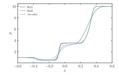
The third hydrodynamics test problem (Problem HD3 in Table 1) is the often-employed shock-tube problem. Here, the simulation domain spans with and . In this problem, the initial discontinuity decays into a left-propagating rarefaction wave and a right-propagating shock wave. The contact discontinuity adjacent to the shock wave also propagates to the right. The left panel of Fig. 4 shows the rest-mass density profile at the end of the simulation for which the contact discontinuity is located at . In this problem, we find that there is no qualitative difference between the numerical solutions with the two solvers irrespective of the cell reconstruction accuracy. This behaviour is also reported in Ref. Mignone and Bodo (2005). For obtaining an accurate result for this particular shock-tube problem it is necessary to employ an accurate reconstruction method. This suggests that employing an accurate reconstruction method is as important as employing an accurate solver in numerical hydrodynamics at least in the one-dimensional problems.
For the fourth (final) hydrodynamics test problem (Problem HD4), we employ a simulation domain of with a grid spacing of , i.e., . The solution consists of a left-propagating rarefaction wave and a right-propagating shock wave. Note that the result differs from that in Problem HD3 as the shock is much stronger compared to the one in Problem HD3 because of the initial large pressure jump (see Table I). A right-propagating contact discontinuity appears adjacent to the shock wave. We plot the rest-mass density profile at in the right panel of Fig. 4. We find that the contact discontinuity (located at ) is more sharply resolved with the HLLC solver than with the HLLE solver when we employ 3rd-order reconstruction. We find that the compression parameter for the min-mod function in the PPM cell reconstruction should be reduced to be 1 in this problem (i.e., a steep limiter function does not work; see, e.g., Ref. Shibata and Sekiguchi (2005)). Otherwise, spurious waves appear irrespective of which solver is used (not shown).
IV.1.2 Magnetohydrodynamics: one-dimensional shock tubes
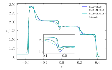
In this section we consider six special relativistic magnetohydrodynamics test problems in one spatial dimension. All the test problems except for Problem MHD6 are carried out in a domain of size with grid spacing (i.e., ). For Problem MHD6, the domain is identical but we employ a higher resolution with and .
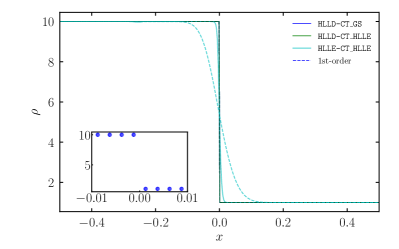
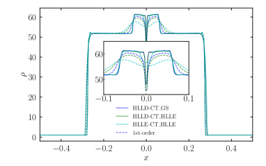
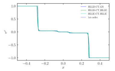
In the first problem (Problem MHD1 in Table 1) the solution consists of a stationary contact discontinuity. The left panel of Fig. 5 plots the rest-mass density profile at the end of the simulation. Because the HLLD-CT_GS and HLLD-CT_HLLE solvers exactly capture the contact discontinuity, the numerical solutions remain stationary even when we employ 1st-order reconstruction (see the inset in the left panel of Fig. 5). On the other hand, with the HLLE-CT_HLLE solver, the initial contact discontinuity is broadened because this solver neglects the contact discontinuity inside the Riemann fan. However when we employ 3rd-order (PPM) reconstruction, this spurious broadening of the contact discontinuity is suppressed, although the contact wave is still not resolved as sharply as it is with the HLLD solver.
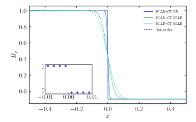
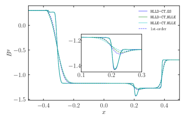
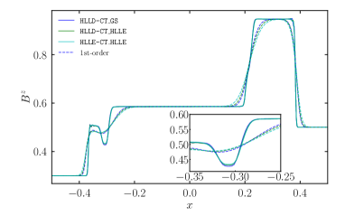
In the second magnetohydrodynamics test problem (Problem MHD2 in Table 1) we model a stationary rotational discontinuity (i.e., an Alfvén wave). The right panel of Fig. 5 presents the profile of the -component of the magnetic field at the end of the simulation. When we employ 1st-order cell reconstruction, the HLLD-CT_GS solver reproduces the stationary solution (see the inset in the right panel of Fig. 5). This is because the rotational discontinuity is captured exactly by the HLLD solver, and the electric field at the cell edge is evaluated with the numerical flux, i.e., the electric field at the cell interface, given by the HLLD solver with the CT_GS scheme (see, e.g., Eq. (179)). With the HLLD-CT_HLLE solver, on the other hand, the rotational discontinuity is broadened because the electric field at the cell interface given by the HLLD solver is not used to evaluate the electric field at the cell edge in the CT_HLLE scheme. With the HLLE-CT_HLLE solver, the rotational discontinuity inside the Riemann fan is not captured. As a result, the initial rotational discontinuity is spuriously broadened. This drawback is improved by employing 3rd-order PPM cell reconstruction in the HLLD-CT_HLLE and HLLE-CT_HLLE solvers. Note that for this problem, we employ the compression parameter in the min-mod function for the PPM reconstruction in the HLLD-CT_GS run. Otherwise, we find the over- and under-shoot in the vicinity of the initial rotational discontinuity (not shown) because the default value of is not sufficient to capture the initial steep profile.
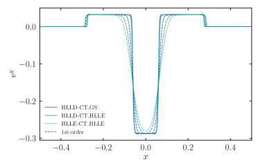
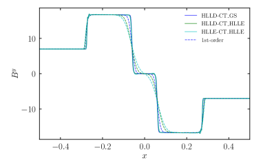
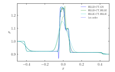
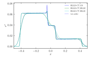
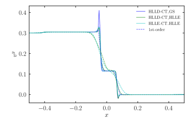
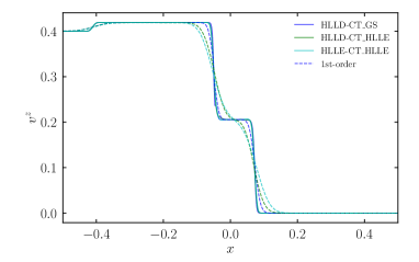
The third magnetohydrodynamics test problem (Problem MHD3) is the relativistic extension of the Brio-Wu shock tube Brio and Wu (1988). In this problem, the solution consists of a left-propagating rarefaction wave, a right-propagating slow shock wave (located at in Fig. 6), and a right-propagating rarefaction wave. In addition there is a right-ward propagating contact discontinuity located at in Fig. 6 adjacent to the shock wave. Finally at , a compound wave appears. When we use 1st-order reconstruction, the contact discontinuity is captured more sharply with the HLLD-CT_GS solver than with the HLLD-CT_HLLE solver, while the HLLE-CT_HLLE solver cannot capture the contact discontinuity at all if the 1st-order reconstruction is used. The slow shock is also captured more sharply with the HLLD-CT_GS solver than with the HLLD-CT_HLLE solver, while with the HLLE-CT_HLLE solver the slow shock wave is significantly broadened. This feature is also found for the compound wave. While the various waves are better captured in 3rd-order PPM reconstruction irrespective of the chosen solvers, we find that the higher order reconstruction method induces artificial oscillatory behavior behind the compound wave (in the regions of ) in both the rest-mass density and in the -component of the velocity (see also in the regions of in the -component of the velocity). The amplitude of these oscillations is reduced when we employ the diffusive compression parameter of the PPM reconstruction .
The fourth magnetohydrodynamics test problem (Problem MHD4) consists of a left (right)-propagating fast wave located at , a left-propagating rarefaction wave (), a contact discontinuity (), a right-propagating slow wave (), and, finally, a left (right)-propagating Alfvén wave (located at ). See Fig. 7 for the solutions (the inset in the () panel shows a close-up region of the right (left) Alfvén waves). When we employ 1st-order reconstruction, both solvers are able to capture the fast waves, but the contact discontinuity is captured more sharply with the HLLD-CT_GS or HLLD-CT_HLLE solver than with the HLLE-CT_HLLE solver (see the inset in the rest-mass density profile in Fig. 7 which shows a close-up of the contact discontinuity). Irrespective of the solvers, it is hard to distinguish the slow wave and the right-propagating Alfvén wave, and also between the the rarefaction wave and the left-propagating Alfvén wave. When we employ 3rd-order PPM reconstruction, on the other hand, we find no qualitative difference in the numerical solutions between the different solvers.
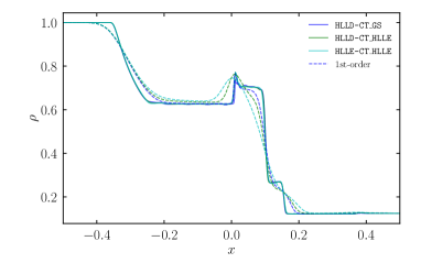
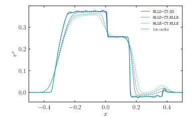
For our fifth magnetohydrodynamics test problem (Problem MHD5) we consider the relativistic collision of two streams. Figure 8 shows the result at . In this problem the solution consists of left (right)-propagating fast waves located at , and left (right)-propagating slow waves located at . When we employ 1st-order cell reconstruction, the slow waves are captured more sharply with the HLLD solvers, i.e., the HLLD-CT_GS or HLLD-CT_HLLE solvers than with the HLLE-CT_HLLE solver. On the other hand, the resolution across the outermost fast waves is essentially the same for all solvers. Irrespective of the solver or reconstruction method used, a spurious undershoot in the rest-mass density appears at . This is known as the wall-heating problem Noh (1987): it is well-known that Godunov-type schemes cannot avoid this pathological behavior. As reported in Ref. Mignone et al. (2009), the undershoot is shallower with the HLLE-CT_HLLE solver due to the solver’s larger numerical diffusion. When we employ 3rd-order PPM reconstruction, both the HLLD and HLLE solvers are equally capable of capturing the slow waves as well as the fast waves.
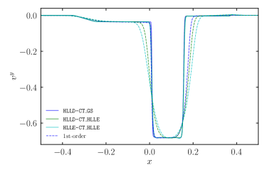
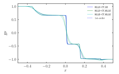
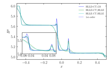
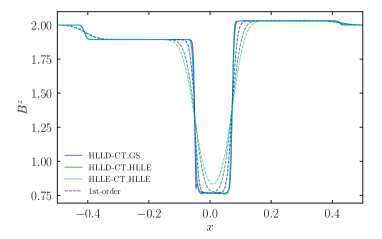
In the final problem (Problem MHD6) in our one-dimensional suite, the solution consists of all seven waves Giacomazzo and Rezzolla (2006). The numerical results are shown in Fig. 9. In this problem, a contact discontinuity appears at , a rarefaction wave propagates to the left of the contact discontinuity, which can be seen at , and the rotational discontinuity at and the slow shock at follow the rarefaction wave (see the inset in the panel for in Fig. 9). To the right of the contact discontinuity, a fast shock propagates up to . The rotational discontinuity at and the slow shock at follow the fast shock (again, this is most easily seen in the inset in the panel for in Fig. 9).
When we use 1st-order cell reconstruction (dashed curves), the contact discontinuity is resolved only with the HLLD solvers, i.e. HLLD-CT_GS or HLLD-CT_HLLE, (see the panel for in Fig. 9). With 1st-order reconstruction, however, it is difficult to disentangle the left/right-propagating rotational discontinuities and left/right-propagating slow shocks, even with the HLLD solver (see the dashed curves in the inset in the panel for in Fig. 9). When we employ 3rd-order PPM reconstruction (solid curves), on the other hand, the difference between the various Riemann solvers is striking. With the HLLD-CT_GS solver, the left/right-propagating rotational discontinuities and slow shocks are captured as plotted in the inset in the panel for in Fig. 9. With the HLLD-CT_HLLE or HLLE-CT_HLLE solvers, the right-propagating rotational discontinuity and the left/right-propagating slow shock are captured, but the left-propagating rotational discontinuity is not. This demonstrates the ability of the HLLD-CT_GS solver to properly capture all seven of the emergent waves.

IV.2 Special relativistic multi-dimensional problems
IV.2.1 Hydrodynamics: two-dimensional shock tube
For our first multi-dimensional special relativistic test problem, we consider the two-dimensional Riemann problem first proposed in Ref. Zanna and Bucciantini (2002). The simulation domain spans in both the - and -directions. We set and . We impose outflow boundary conditions in both directions. We use an adiabatic index of . We employ 3rd-order PPM reconstruction and set the CFL number to be 0.45. Finally, the initial condition is given by
| (186) |
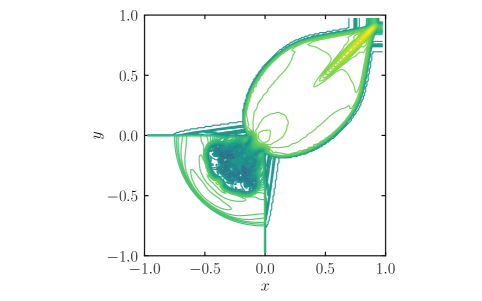
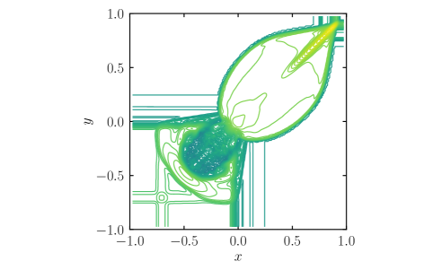
Figure 10 show the logarithmic contour of the rest-mass density at with the HLLC solver (left panel) and with the HLLE solver (right panel). The most notable difference in the solutions between the two solvers appears around the two tangential discontinuities in the lower-left portion of the simulation domain. With the HLLC solver (left panel), the initial tangential discontinuities remain sharp. With the HLLE solver, on the other hand, spurious waves propagate along each axis from the initial tangential discontinuities due to numerical diffusion. Unlike the one-dimensional problems, the spurious diffusion out of the initial tangential discontinuities that occurs with the HLLE solver cannot be mitigated even when we employ 3rd-order PPM reconstruction. Thus in this multi-dimensional test problem we observe a qualitative difference in the solutions between the HLLC and HLLE solvers that cannot be removed by resorting to higher-order reconstruction.
IV.2.2 Hydrodynamics: two-dimensional cylindrical explosion
For the second special relativistic multi-dimensional test problem, we consider a cylindrical blast wave in two dimensions. For this problem, we choose the simulation domain to span and , and set , i.e., in the - and -directions, respectively. Periodic boundary conditions are imposed at the - and -boundaries. We set the adiabatic index to , employ 3rd-order PPM reconstruction, and set the CFL number to 0.45. The initial condition is given by
| (189) |
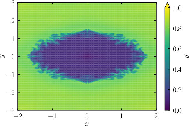
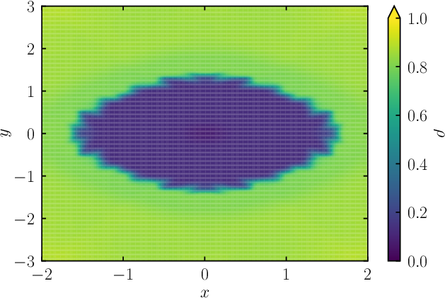
Figure 11 shows the rest-mass density profile at with the HLLC solver (left panel) and the HLLE solver (right panel). By this time, the blast wave has intersected itself many times, and consequently a Rayleigh-Taylor-like instability (known in this context as the Richtmyer-Meshkov instability) has developed White et al. (2016). With the HLLC solver, the Richtmyer-Meshkov instability is well resolved, and as a result the density irregularity around the elliptical figure is sharply captured. By contrast, with the HLLE solver, the fine structure around the elliptical figure is not captured well due to the large numerical diffusivity. This demonstrates an effective improvement in spatial resolution with the HLLC solver compared to that with the HLLE solver.
IV.2.3 Magnetohydrodynamics: two-dimensional magnetized current sheet
Next we consider a two-dimensional problem in relativistic magnetohydrodynamics: that of a magnetized current sheet, studied recently by Refs. Mignone and Del Zanna (2021); White et al. (2016). The initial profile for the magnetic field is given by
| (190) |
where and . The density is uniform with and the fluid is at rest with . The thermal pressure is determined from the force balance with the magnetic pressure and its profile is given by
| (191) |
where is the initial plasma-beta parameter, which we set to unity. The equilibrium magnetic field is initially perturbed and the perturbation is given by the -component of the vector potential as
| (192) |
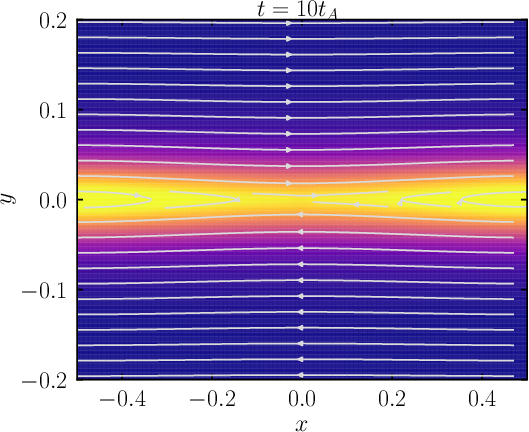
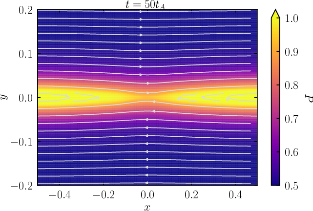
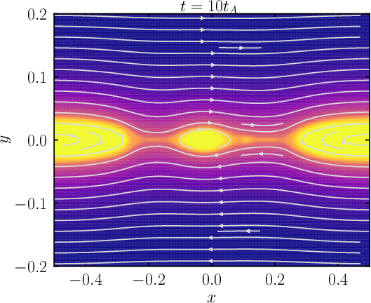
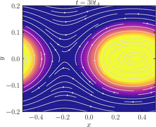
where , , , and and denote the domain size in the - and -directions, respectively. We employ a simulation domain consisting of and . To check convergence, we carry out simulations at three different resolutions: , , and . We set the CFL number to 0.8 in all simulations. We impose a periodic boundary condition in the -direction, and a reflective boundary condition in the -direction. With this setup, the maximum Alfvén wave speed is and the Alfvén timescale is .
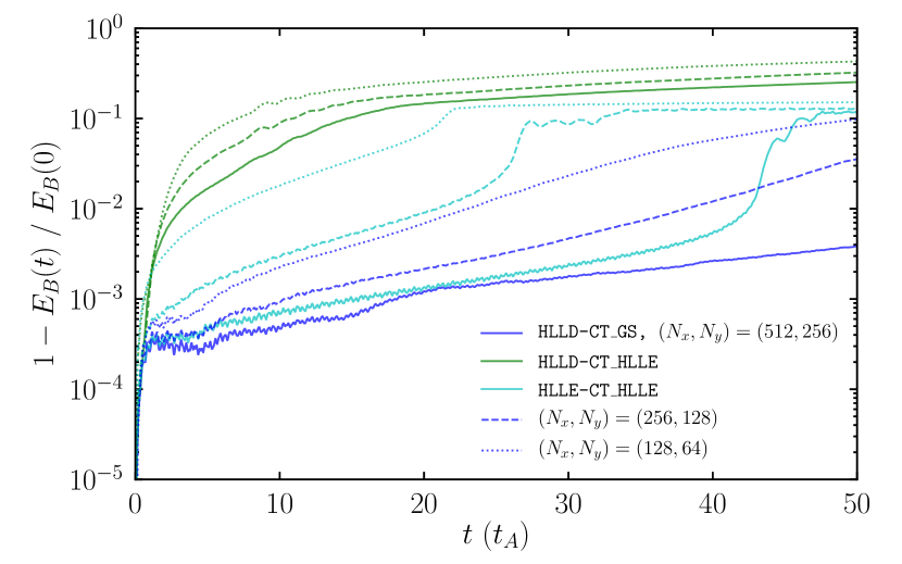
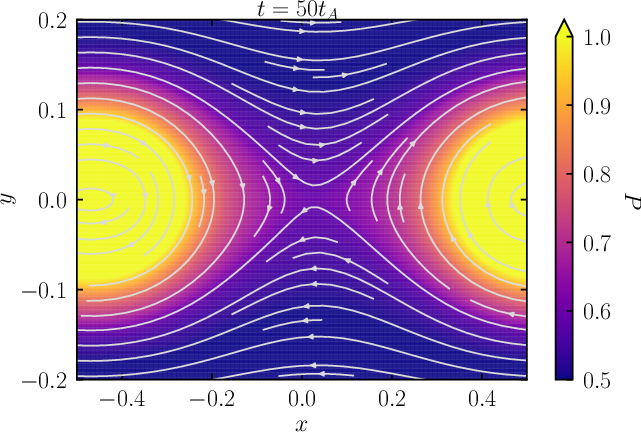
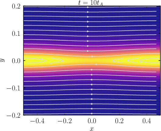
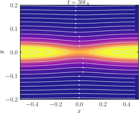
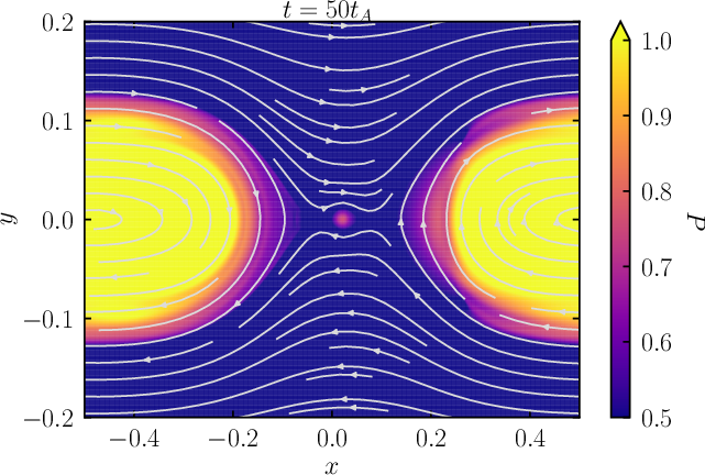
Figure 12 displays colorplots of the thermal pressure together with the magnetic-field lines at three different times: (left panel), (center), and (right). The top, middle, and bottle panels show the numerical solutions with the HLLD-CT_GS, HLLD-CT_HLLE, and HLLE-CT_HLLE solvers, respectively. The snapshots are all taken from our highest resolution runs with . Magnetic field lines reconnect at due to the numerical resistivity inherent both in the Riemann solvers as well as in the constrained transport scheme. Once reconnection starts, the profile of the magnetic-field lines changes, and as a result, the thermal pressure profile is modified, leading to the formation of island-like structures.
The timescale of the reconnection depends on how large the numerical resistivity is. Figure 12 indicates that the HLLD-CT_GS solver is accompanied with the smallest numerical resistivity because the formation of the islands is delayed. It is found that HLLD-CT_HLLE solver has the largest numerical resistivity, leading to rapid formation of the islands. This does not agree with one’s naive expectation, because the HLLE-CT_HLLE solver is actually less dissipative than the HLLD-CT_HLLE solver. In other words, we observe an unexpected hierarchy between the HLLD-CT_HLLE and HLLE-CT_HLLE solvers. This stems from the algorithm of the CT_HLLE solver. In this constrained transport scheme, dissipation terms which are proportional to the maximum absolute value of the characteristic speed appear in the electric-field evaluation (see, e.g., Eq. (44) in Ref. Del Zanna et al. (2003)). This characteristic speed is then obtained from the (global) Riemann solver. We find that the HLLD solver returns a larger characteristic speed than the HLLE solver. As a result, the HLLD-CT_HLLE solver ends up being more diffusive than the HLLE-CT_HLLE solver, as can be seen in this test problem.
Figure 13 shows the fraction of the initial magnetic-field energy that is dissipated as a function of time. With the HLLD-CT_GS solver (blue curves), the magnetic-field energy dissipates only gradually. Also, the dissipation rate is suppressed when we employ higher resolution: the energy increases by an order of magnitude only over Alfvén timescales. This feature is also found for the HLLE-CT_HLLE solver (cyan curves), although the dissipation rate steeply rises at a later time, , even in our highest resolution run. With the HLLD-CT_HLLE solver (green curves), magnetic reconnection commences immediately after the simulation starts. We conclude that for problems involving strong magnetic field gradients (current sheets) accurate evolution can be modeled only when the HLLD solver is paired with CT_GS for the constrained transport.
IV.2.4 Magnetohydrodynamics: two-dimensional Kelvin-Helmoltz instability
The second two-dimensional problem in special relativistic magnetohydrodynamics is the Kelvin-Helmholtz instability, as proposed in Refs. Mignone et al. (2009); Bucciantini and Del Zanna (2006). For this, we prepare a simulation domain which spans and . To check the convergence, we perform the simulations with three different resolutions: (‘high’ resolution), (‘medium’ resolution), and (‘low’ resolution). The simulations are carried out with either the HLLD-CT_GS or HLLE-CT_HLLE solvers, and we employ 3rd-order PPM reconstruction for all the simulations. We impose a periodic boundary condition in the -direction, and an outflow boundary condition in the -direction. The CFL number is set to 0.4 in all the simulations.
As the initial condition, we give a tanh-shaped shear velocity profile for the -component,
| (193) |
where and . The thickness of the shear layer is covered by around and grid cells at the low, medium, and high resolutions, respectively. We employ a uniform density of , and a uniform gas pressure with . The adiabatic index is taken to be . Note that our setup is different from that employed in the recent test simulation for the Kelvin-Helmholtz instability in special relativistic magnetohydrodynamics of Ref. Mattia and Mignone (2021), in which the authors employ a non-uniform density field, a smaller shear-layer thickness of , and an amplitude of the -component of the velocity () which is twice that used in our runs.
The magnetic field at is given by
| (194) |
i.e. the magnetic field is initially uniform and parallel to the velocity in the lower-half of the -plane. We set . The shear layer is perturbed by the motion in the -direction as
| (195) |
while .
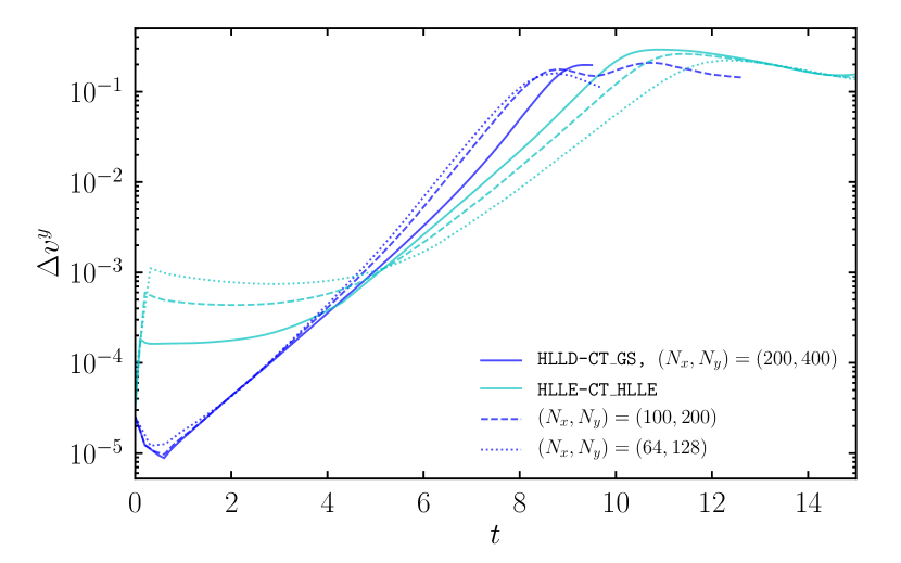
Figure 14 shows the perturbed velocity difference as a function of time taken from six simulations at three different resolutions and employing either the HLLD-CT_GS or HLLE-CT_HLLE solver. All the simulations start from perturbations of size . We find exponential growth followed by nonlinear saturation at the end of the linear phase at . The behavior during the linear phase depends strongly on the solver, particularly at low resolutions. Nonlinear saturation occurs more quickly in the simulations with the HLLD-CT_GS solver than in those with the HLLE-CT_HLLE solver, but the saturation amplitude depends only weakly on the solver and resolution. The growth rate is higher with the less diffusive HLLD-CT_GS solver than with the HLLE-CT_HLLE solver, but the results converge between the two solvers as the resolution is improved. This result is consistent with that in Ref. Mattia and Mignone (2021) (see their Fig. 14). The evolution after the nonlinear saturation is not sensitive to the solver or resolution, although at late times (not shown) the velocity difference decays more quickly in the simulations with the (more diffusive) HLLE-CT_HLLE solver than with the HLLD-CT_GS.
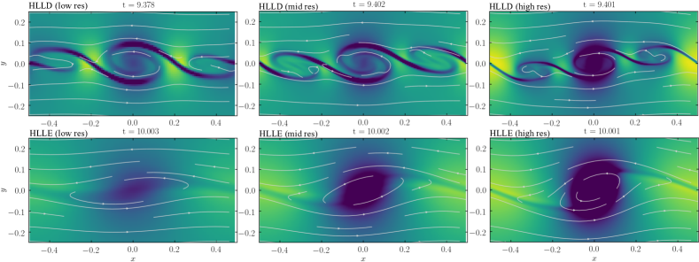
In Fig. 15 we show snapshots of the density at nonlinear saturation from the six simulations. The top row shows results from the low, medium, and high resolution runs using the HLLD-CT_GS solver, while the bottom row shows the corresponding snapshots from runs that employ the HLLE-CT_HLLE solver. Using the HLLD-CT_GS solvers, we observe the formation of a single vortex together with two neighboring, stretched secondary vortices that are well-resolved at all resolutions, whereas with the HLLE-CT_HLLE solver we see the formation of only a single large vortex at the shear interface, mirroring the behaviour of the Kelvin-Helmholtz instability in the simulations of Ref. Bucciantini and Del Zanna (2006) which employed the HLLE-CT_HLLE solver. Our results show that, at least at low resolutions, the HLLE solver is not appropriate for studying phenomena in which the Kelvin-Helmholtz instability plays an important role.
IV.3 General relativistic problems in a fixed background spacetime
IV.3.1 Hydrodynamics: Bondi flow
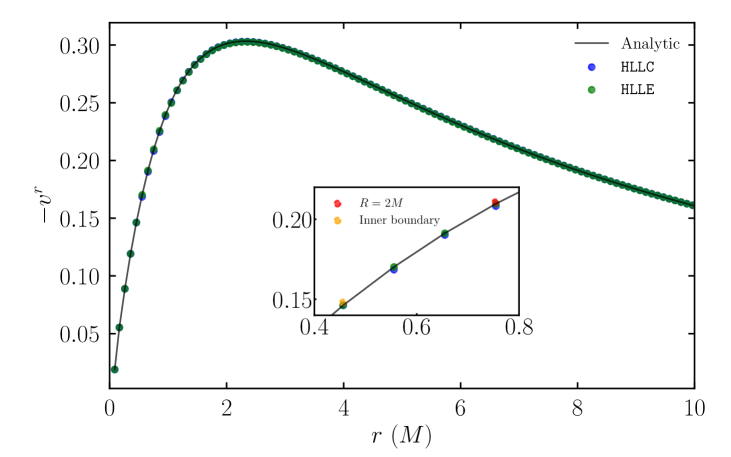
As a test problem in a curved (but static) spacetime, we consider spherical accretion (ingoing Bondi flow) onto a non-rotating black hole Hawley et al. (1984). The Bondi flow in Schwarzschild coordinates has been extensively discussed in the literature (see, e.g., Ref. White et al. (2016)). Following previous work Gammie et al. (2003); Shibata and Sekiguchi (2005), we adopt the parameters for this problem as follows: an adiabatic index of , an adiabat of , and a critical radius of , where denotes the black hole mass. With this setup, the mass accretion rate is 0.797. We perform simulations both with the HLLE and HLLC solvers, and employ 3rd-order PPM reconstruction.
Our numerical-relativity code employs the so-called puncture formalism, and hence, in the presence of black holes, the black-hole spacetime is foliated in most cases by the so-called limiting hypersurface Estabrook et al. (1973). Thus, for preparing a practical setup in this test problem, a non-rotating black hole should be described in the so-called maximal trumpet geometry rather than in Schwarzschild coordinates or in isotropic coordinates on slices of constant Schwarzschild time Baumgarte and Naculich (2007); Miller and Baumgarte (2017). Note that in both of these latter two coordinate systems, the fluid four-velocity exhibits pathological behavior near the horizon Miller and Baumgarte (2017) 333The pathological behavior at the horizon is avoidable if one employs Kerr-Schild coordinates. However, we employ the maximal trumpet geometry in this test problem because of its high compatibility with our numerical relativity code.. In Appendix B, we describe the explicit coordinate transformation from the Schwarzschild coordinates to the maximal trumpet geometry. With this geometry, the radial component of the shift vector is non-zero. Therefore, the tetrad basis (see, e.g., Eq. (60)) does not agree any longer with a coordinate basis in the Minkowski spacetime, and the cell interface may be dragged by the shift vector as discussed in Sec. III.2.
We employ a simulation domain in Cartesian coordinates spanning with . The grid spacing of the simulation is given by with as the number of grid cells in each direction. We also check convergence by increasing the resolution to and , which correspond to grid spacings of and , respectively. We set the CFL number to 0.45 and integrate the numerical solution up to . We impose a stationary boundary condition at the outer and inner boundaries, with the latter located at . Note that the horizon in this geometry is located at . We also impose octant symmetry at the , and planes.
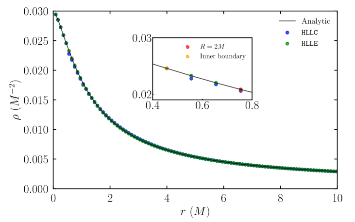
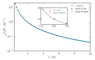
Figure 16 shows radial profiles of the rest-mass density and the radial velocity calculated by the HLLC solver with the blue dots and by the HLLE solver with the green dots on top of the analytic solution Hawley et al. (1984). The profiles are along the diagonal direction, i.e., in the simulation domain. This figure demonstrates that our implementation of the HLLC solver in curved spacetime works well. It also shows that, for this particular problem, the HLLE solver works as well as the HLLC solver because of the smoothness of the accretion flow, as many other previous implementations have shown; e.g., Refs. Gammie et al. (2003); Shibata and Sekiguchi (2005); Mösta et al. (2014); Etienne et al. (2010).
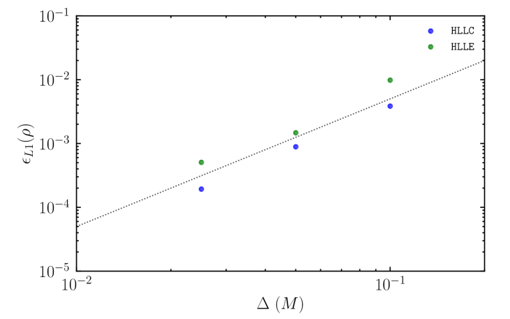
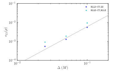
In the lower panel of Fig. 16 we plot the norm of the error in the rest-mass density as a function of the spatial grid spacing. The convergence order of the norm of the error is both for the HLLC and HLLE solvers, because our Riemann solver is 2nd-order accurate. One likely reason for the slight deviation from the expected accuracy is that spherical symmetry of the accretion flow is not perfectly preserved during the evolution because we simulate it in the Cartesian geometry. This plot also shows that the numerical solution with the HLLC solver is more accurate than that with the HLLE solver. Our interpretation of this is that with the tetrad transformation (see Sec. III.2) the frame-dragging effect of the cell interface is taken into account with a better accuracy (see also Fig. 2) 444Note that our HLLE solver (which was the only Riemann solver present in our original formulation), does not employ the tetrad transformation, but is instead formulated directly in a curved spacetime. See Ref. Shibata and Sekiguchi (2005) for details..
IV.3.2 Magnetohydrodynamics: Magnetized Bondi flow
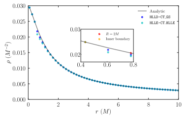
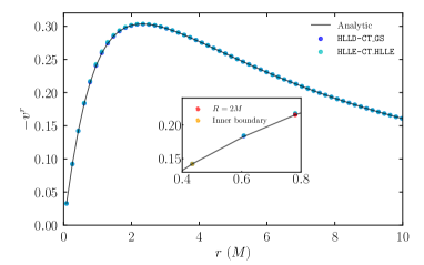
The next test problem in a curved spacetime is magnetized Bondi flow onto a non-rotating black hole. It is known that a purely radial magnetic field does not alter the flow profile of non-magnetized Bondi flow Shibata (2016). Therefore, we employ the same flow profile used in the previous section. From the divergence-free condition (17), the radial magnetic field should be in Schwarzschild coordinates (see Appendix B for the definition of and the transformation to the maximal trumpet geometry). The amplitude of the magnetic field is chosen to be such that at . We perform two simulations, one with the HLLD-CT_GS solver and the other with the HLLE-CT_HLLE solver. We employ RK4 and 3rd-order PPM reconstruction in both cases.
We employ a simulation domain in Cartesian coordinates spanning with . The grid spacing of the simulation is with being the number of the grid cells in each direction. To check convergence, we perform better-resolved simulations with and , i.e., and , respectively. We impose octant symmetry at the , , and planes, and a stationary condition at the outer and inner boundaries, with the latter located at . Numerical simulations are performed up to .
Figure 17 shows the radial profiles of the rest-mass density (top-left), the radial velocity (top-right), and the radial magnetic field (bottom-left). Numerical solutions with the HLLD-CT_GS solver are indicated by the blue dots, while those with the HLLE-CT_HLLE solver are indicated by the cyan dots. As in the non-magnetized cases, the flow profiles agree with the analytic solution Hawley et al. (1984) (see also the insets in Fig. 17 which show the solution close to the inner boundary). The rest mass density inside the horizon slightly deviates from the analytic solution. However, the deviation decreases as the spatial resolution is increased. This demonstrates that our HLLD solver works just as well as our HLLC solver in a curved spacetime. As in the hydrodynamic case, we find no qualitative difference in the numerical solutions between the HLLD-CT_GS and HLLE-CT_HLLE solvers because of the smoothness of the accretion flow. The bottom-right panel in Fig. 17 plots the norm of the error in the rest-mass density as a function of the spatial grid spacing. It shows that (i) the numerical solution with the HLLD-CT_GS solver is more accurate than that with the HLLE-CT_HLLE solver, and (ii) the order of the convergence is . These results are essentially the same as those in the previous subsection. Again, the deviation from the formal accuracy of the Riemann solver is likely to be an artifact of the Cartesian geometry which we employ.
V Application to a dynamical spacetime
Finally, we apply our new Riemann solvers in general relativity to a dynamical spacetime. We simulate a binary neutron star merger, both with and without magnetic fields. We turn on the solver for Einstein’s equations and the neutrino-radiation hydrodynamics solver in the simulations shown in this section (see Eqs. (11)–(15)).
V.1 Hydrodynamics: binary neutron star merger
V.1.1 Setup
First, we consider non-magnetized asymmetric binary neutron stars with masses of and . We utilize the spectral method library LORENE LORENE ; Gourgoulhon et al. (2001); Taniguchi and Shibata (2010); Taniguchi and Gourgoulhon (2002, 2003) to generate a quasi-equilibrium configuration of the irrotational binary neutron star. We also employ an eccentricity reduction prescription to generate an initial condition that has low orbital eccentricity Kyutoku et al. (2014). The initial orbital angular velocity is set to be where is the total mass of the binary.
Our solver for Einstein’s equations implements the BSSN-puncture formulation Shibata and Takashi (1995); Baumgarte and Shapiro (1998); Campanelli et al. (2006); Baker et al. (2006), locally incorporating the Z4c prescription for constraint propagation Hilditch et al. (2013). We employ 4th-order centered finite differencing for the spatial derivative of the metric, a lop-sided finite difference for the advection term associated with the shift vector, and 4th-order Runge-Kutta for the time integrator. For the relativistic hydrodynamics solver, we employ either the HLLC or HLLE solver, together with 3rd-order PPM cell reconstruction.
We employ the SFHo equation of state for relatively high-density nuclear matter Steiner et al. (2013), and the Timmes (Helmholtz) equation of state for the low-density part Timmes and Swesty (2000). Because high-resolution shock-capturing schemes cannot treat the vacuum state, we need to implement an artificial atmosphere outside the neutron stars. In this simulation, we set a constant atmospheric density of for the inner part of the finest fixed mesh refinement (FMR) domain, for which the refinement boundary along each axis is typically located at (see below for the FMR setup in detail). We also set a power-law profile of the atmospheric density of for and as far as the atmospheric density is larger than the floor value which is determined by the employed equation of state. In our present table for the equation of state, this floor is and if becomes smaller than this value, we set the the atmospheric density to the floor value. The atmospheric temperature is set to be .
We also explicitly solve the radiation-hydrodynamics equations for neutrinos in time using an approximate neutrino-transfer scheme based on a leakage scheme Sekiguchi (2010) and the truncated moment formalism Thorne (1981); Shibata et al. (2011). The cooling source terms are computed using a general-relativistic leakage scheme Sekiguchi et al. (2012), and heating source terms due to neutrino capture processes are computed by the method presented in Ref. Fujibayashi et al. (2017).
The computational region consists of levels of FMR half-cubic domains. The size of each FMR domain is for and , and with . Note that in the -direction we impose reflection symmetry with respect to the equatorial plane, . We set the overall domain size to and . Thus the grid spacing of the finest FMR domain is m. To check convergence, we also perform simulations with lower resolutions of and , for which the grid spacing of the finest FMR domain is m and m, respectively. For the HLLC solver, we perform an additional simulation with and m. By virtue of the cell-centered grid structure, the cell interface of the parent FMR domain coincides with that of the child FMR domain. We employ the reflux prescription during time marching of the Berger-Oliger type mesh refinement algorithm to ensure the conservation of baryonic mass.
V.1.2 Inspiral phase
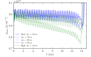
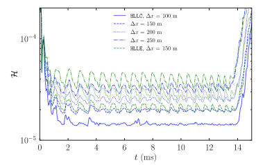
The left and right panels of Fig. 18, respectively, show the time-evolution (during the inspiral phase) of the maximum rest-mass density and the density-weighted Hamiltonian constraint violation (see Eqs. (29) and (30) in Ref. Shibata and Sekiguchi (2005) for definitions). The blue and green curves denote the results with the HLLC and HLLE solvers, respectively, and the solid, dashed, dotted, and dot-dashed curves indicate the resolution (i.e. m, m, m, and m, respectively). During inspiral, the maximum rest-mass density oscillates due to numerical error regardless of which solver is used. It also decreases partly due to the numerical error. However, the degree of the decrease is much more prominent with the HLLE solver than it is with the HLLC solver, especially at the coarsest resolution. This is due to the large numerical diffusion inherent in the HLLE solver. Specifically, this solver is more subject to spurious broadening of the density profile near the stellar surface (not shown), leading to a higher degree of spurious neutron-star expansion and to a resultant decrease in the maximum rest-mass density. However, this artifact is mitigated with the HLLC solver, because of its stronger capability of capturing irregular surfaces, i.e., the stellar surface.
The right panel of Fig. 18 shows that, for a given grid resolution, the time-averaged value of the constraint violation during the inspiral phase is smaller with the HLLC solver than with the HLLE solver. This demonstrates that the numerical result with the HLLC solver is more accurate than that with the HLLE solver. We find that the order of convergence of the density-weighted Hamiltonian constraint violation is –, irrespective of which Riemann solver is used. Note that this convergence is slow compared to that achieved using a higher-order finite difference scheme Bernuzzi and Dietrich (2016); Radice et al. (2014); Most et al. (2019), but could be improved if we were to employ a more accurate reconstruction scheme such as MP5 Suresh and Huynh (1997). However, the implementation of such a scheme is beyond the scope of this paper.
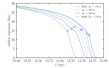
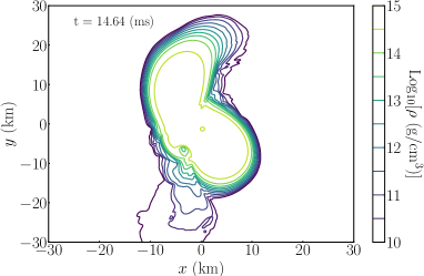
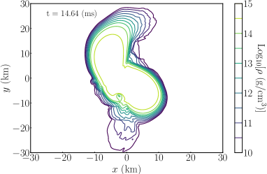
The top panel of Fig. 19 shows the orbital separation of the binary as a function of time. Here we define ‘orbital separation’ as the coordinate distance in the orbital plane between the two rest-mass density maxima. The cross symbols denote the final moment at which we can unambiguously identify the two rest-mass density maxima. At this point the less massive neutron star has been significantly tidally elongated, and we define this time as being the time of onset of the merger. This plot shows that the merger time found in the simulation with the HLLC solver is later than that with the HLLE solver (the reason for this will be described shortly). The bottom panels display contour plots of the rest-mass density in the orbital plane at the moment of merger for the runs with the HLLC solver (left panel) and the HLLE solver (right panel) (for both cases, m). The orbital phase with the HLLE solver slightly larger compared to that with the HLLC solver. This implies that the neutron star simulated with the HLLE solver is more subject to artificial tidal deformation than the neutron star with the HLLC solver, because the HLLE solver (since it cannot accurately resolve the irregularities at the stellar surface) results in a larger spurious expansion of the neutron star. Note that the tidal elongation of the low-density part of the less massive neutron star is more enhanced with the HLLE solver than with the HLLC solver, as found from the comparison of the two contour plots. It is this enhanced (but artificial) tidal elongation with the HLLE solver that ultimately results in the earlier merger time observed when when we employ that solver.
V.1.3 Post-merger phase
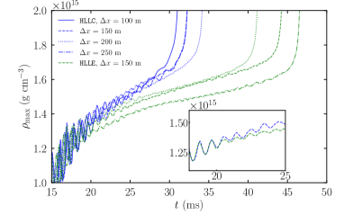
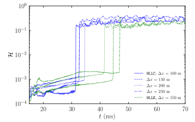
Having presented various diagnostics from the inspiral phase, we now turn our attention to the post-merger phase. Figure 20 shows the maximum rest-mass density and the density-weighted Hamiltonian constraint violation as functions of time during the post-merger phase. The existence of oscillations in the density after the merger indicates the formation of a massive neutron star remnant rather than a direct collapse to a black hole. The remnant massive neutron star gradually contracts due to angular momentum transport by the gravitational torque, neutrino cooling, and gravitational-wave emission. Eventually the remnant collapses to a black hole, indicated by the blow-up of the maximum rest-mass density (see the figure at – ms). Because the remnant massive neutron star is a meta-stable object, its stability is influenced significantly by the numerical truncation error, by the randomness with which the collapse time does not become a monotonic function of the spatial grid spacing. (The non-monotonic behavior of the black-hole formation time with respect to the grid spacing is also reported in the literature (see, e.g, Ref. Baiotti and Rezzolla (2017)).) Specifically, with the HLLC solver, the collapse time of the remnant coincides for both the m and m runs, is earliest for the m run, and is latest for the m run. With the HLLE solver, the collapse time is earliest for the m run and the latest for m run. The inset in the left panel of Fig. 20 shows a close-up of the results with the HLLC and HLLE solvers for m.
However, the collapse time of the remnant is systematically earlier for runs with the HLLC solver. This is related to the evolution of the oscillation amplitude of the remnant neutron star. For ms, the oscillation amplitude of the maximum rest-mass density is approximately identical for the two solvers (see the left-hand panel of Fig. 20). After that, however, the oscillations are noticeably damped when we use the HLLE solver. This implies that the oscillation energy is dissipated by the numerical diffusion inherent in the HLLE solver. Thus, the lifetime of the remnant massive neutron star is significantly overestimated when the more diffusive HLLE solver is used.
The right panel of Fig. 20 shows that the density-weighted Hamiltonian constraint violation is of order during the remnant massive neutron star phase and of order after the black hole formation. The constraint violation only slowly decreases with increased resolution in the post-merger phase, and does so regardless of which solver is used. The reason for this is that during the merger phase, shocks are formed inside a large portion of the neutron stars. Because shocks are always computed with first-order accuracy in numerical hydrodynamics, the overall accuracy of the solution deteriorates and the convergence becomes slow.
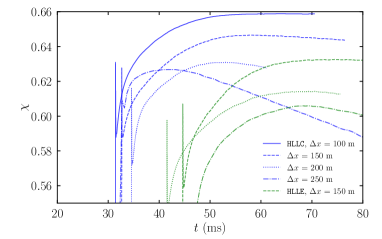
The left panel of Fig. 21 shows the evolution of the dimensionless spin of the remnant black hole 555The methods we use to estimate the non-dimensional spin and the mass of the black hole are the same as in Refs. Kiuchi et al. (2009); Shibata and Taniguchi (2008).. We find spurious spin-down of the black hole due to numerical diffusion, in particular when the simulations are performed at low resolutions with m or m. We measure the spin-down rate in the HLLC run and estimate that the dimensionless spin decreases by in 1 s if where denotes the minimum radius of the apparent horizon. However, the spurious spin-down rate decreases approximately at the 4th order, reflecting the order of the accuracy in the solver for Einstein’s equations. This implies that the spurious decrease of the dimensionless spin will be suppressed to the required level if we perform a simulation with a sufficiently high resolution. In low-resolution runs, however, the spurious spin down will influence the evolution of the disk because the specific angular momentum at the inner stable circular orbit will increase as a result of the spin-down, which in turn will result in spurious mass accretion. Thus the grid resolution must be chosen carefully when the main aim is to quantitatively explore the evolution of the disk and subsequent mass ejection.
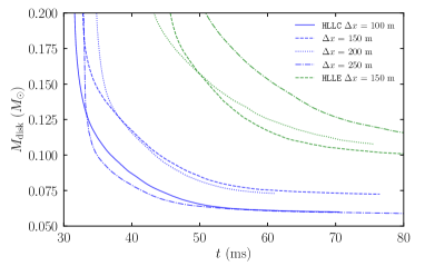
The right panel of Fig. 21 shows the gravitationally bound baryonic mass outside the apparent horizon 666We employ the geodesic criterion to identify gravitationally bound fluid (conversely, corresponds to unbound fluid elements) Hotokezaka et al. (2013).. Irrespective of which Riemann solver we employ, the bounded baryonic mass is not a monotonic function of the grid spacing. Before the formation of the black hole, the non-axisymmetric density structure of the remnant massive neutron star exerts a gravitational torque on the fluid elements. As a result, angular momentum is transported outwards. Thus the longer lifetime of the remnant massive neutron star results in the formation of a more massive torus after the neutron star remnant collapses to the black hole. Because the lifetime of the remnant massive neutron star is not a monotonic function of the grid spacing it is a natural consequence that we find that the baryonic mass of bound material does not converge as the resolution is increased. Nevertheless, in the simulations with the HLLC solver, the gravitationally bound baryonic mass is found to lie in a narrow range, between and , at the time of formation of the black hole (at ms). When we employ the HLLE solver, the bound baryonic mass is systematically larger than that with the HLLC solver (between and ). This is because the lifetime of the remnant massive neutron star is systematically longer in the simulations with the HLLE solver than with the HLLC solver, as already mentioned. Therefore, when one employs the HLLE solver, one should keep in mind that the bound baryonic mass could be overestimated with a systematic error of .
Figure 22 shows the time-evolution of the luminosity of electron neutrinos (left panel) and of electron antineutrinos (right panel). These plots show that the luminosity increases quickly after merger, reaching a peak value of erg/s for the electron neutrinos and erg/s for the electron antineutrinos at ms. These values agree broadly with our previous results Sekiguchi et al. (2016). After the formation of the black hole, the luminosity quickly decreases because the high density and temperature regions of the remnant massive neutron star are swallowed into the black hole Sekiguchi et al. (2011, 2016). Note that the overall evolution of the neutrino luminosity in the remnant massive neutron star phase does not significantly depend either on the Riemann solver, nor on the spatial grid spacing.
Finally, Fig. 23 shows the time-evolution of the gravitationally unbound baryonic mass, i.e. the ejecta mass. In this model (i.e., the model with appreciable mass asymmetry in the binary), mass ejection is driven primarily by the tidal force from the heavier component to the lighter one. The blue and green curves denote results with the HLLC and HLLE solvers, respectively. The solid, dashed, dotted, and dot-dashed curves denote the results with grid spacings of m, m, m, and m, respectively. The inset depicts the ejecta-mass evolution on a logarithmic scale along the vertical axis, and the shaded region denotes the violation of baryonic mass conservation. We find that the spurious mass ejection during the inspiral phase is , and it decreases as the resolution is enhanced. We also find that the error in baryonic mass conservation is below even after the merger. This figure shows that the ejecta mass decreases as the grid spacing is improved from m to m. This is likely to be related to the spurious expansion of the less massive neutron star during the inspiral phase, which we discussed above. This spurious expansion is enhanced in the lower resolution runs. When we employ m for the HLLC solver, the ejecta mass is approximately identical to that with m. Therefore, the convergence for the ejecta mass is approximately achieved in this model.
Figure 23 also shows that the amount of ejecta mass in the simulation with the HLLC solver is smaller than that with the HLLE solver for a given grid spacing. Quantitatively, the ejecta mass difference due to the Riemann solver is for m in this model. This difference arises from how accurately the employed Riemann solver can capture the neutron-star shape during the late inspiral phase. As we have already emphasized, with the HLLE solver the neutron star spuriously expands during the inspiral phase. As a result, the less massive neutron star is more subject to (partly artificial) tidal deformation, thereby ultimately increasing the tidally-driven ejecta mass. When we employ the HLLC solver together with a high grid resolution this artifact is mitigated. This is one of the advantages of using a more sophisticated Riemann solver in this problem.
We conclude that the HLLC solver is superior to the HLLE solver both during the inspiral and post-merger phases of the binary neutron star merger. In particular, we note that for the purpose of obtaining accurate and high-precision gravitational waveforms during the late inspiral phase over more than 10 orbits, the HLLE solver is likely not an appropriate choice.
V.2 Magnetohydrodynamics: binary neutron star merger (evolution of remnant)
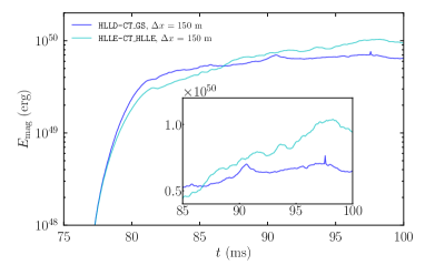
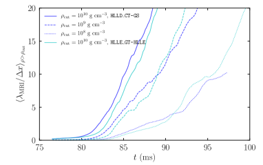
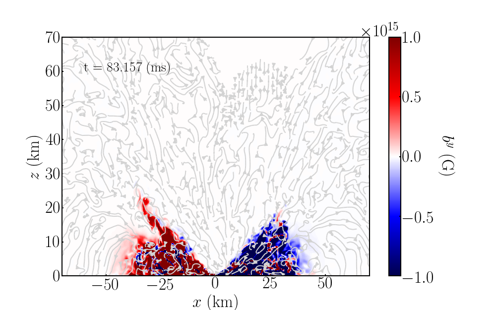
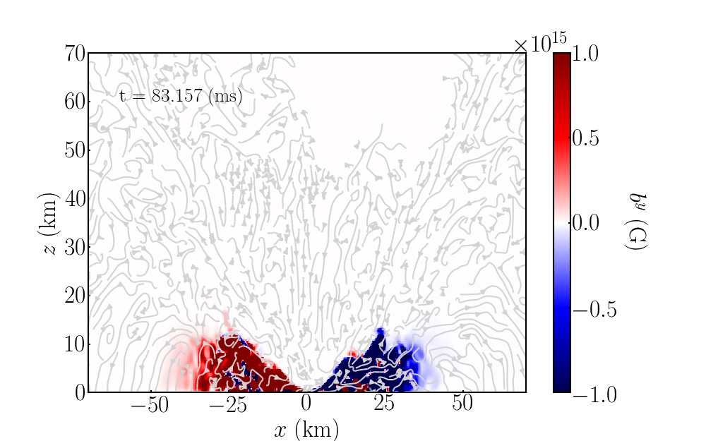
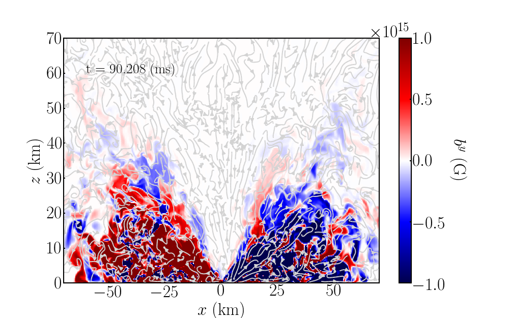
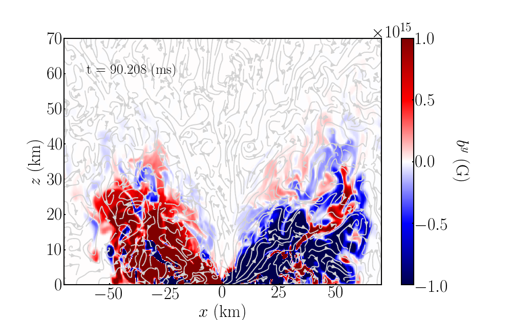
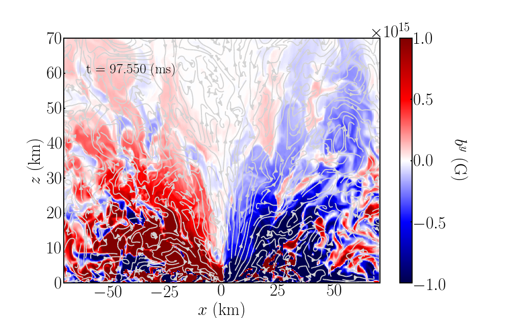
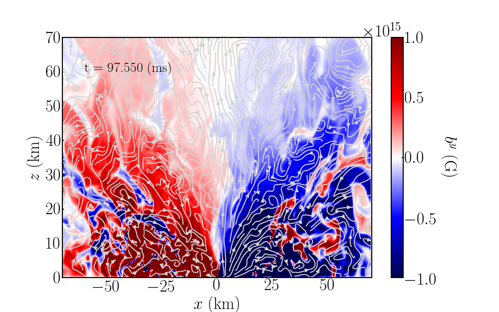
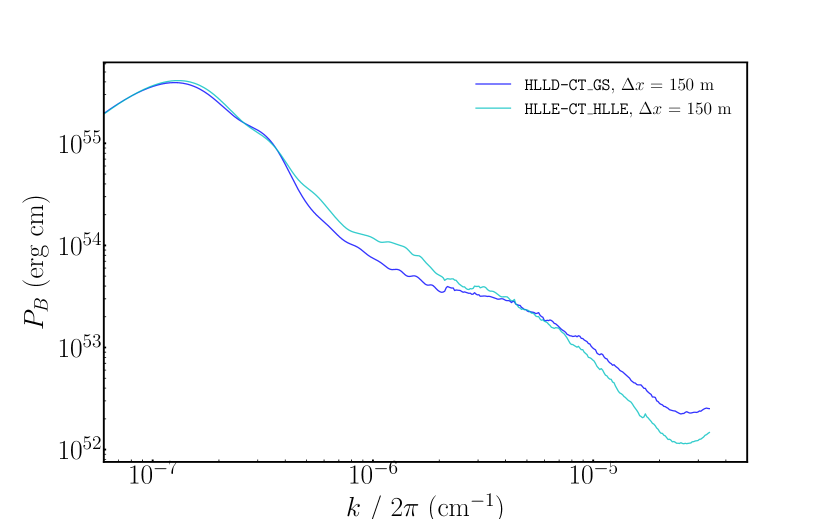
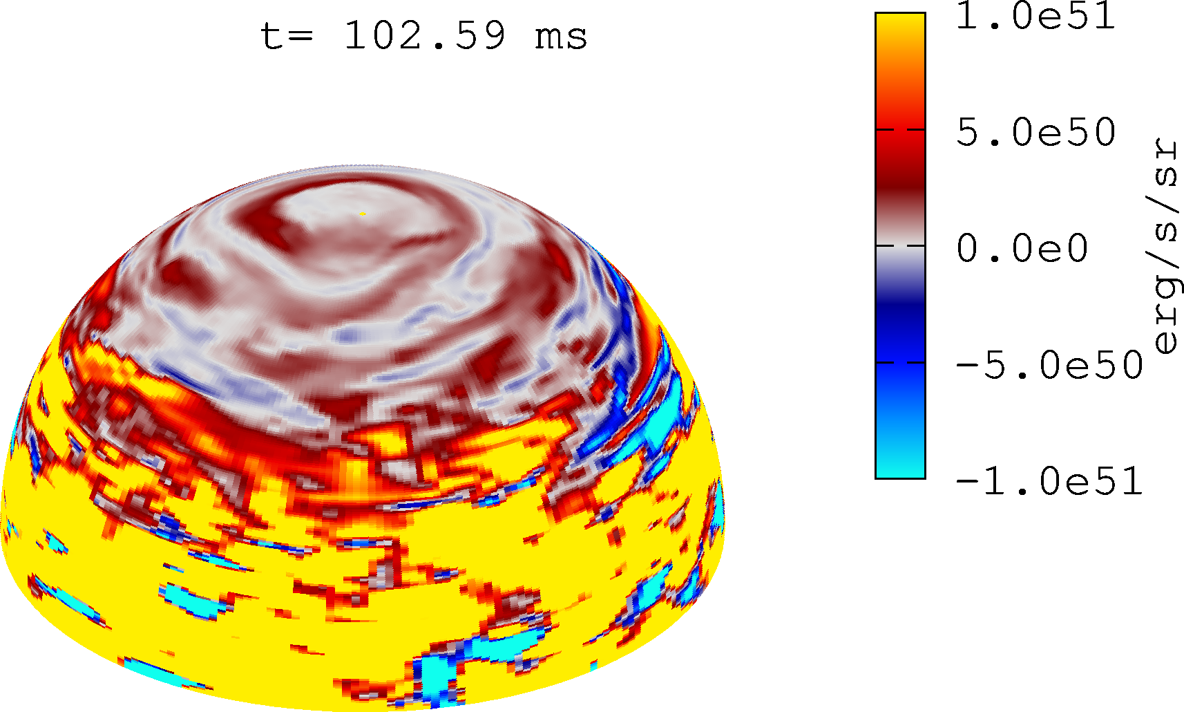
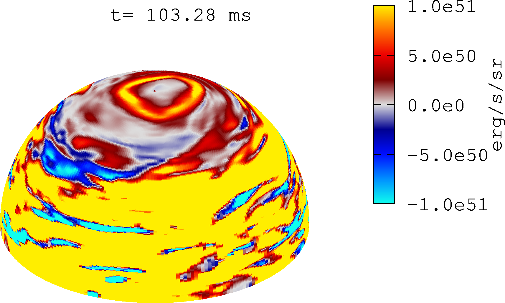
V.2.1 Setup
As an application of the new Riemann solvers (paired with our new implementation of the constrained transport scheme) to relativistic magnetohydrodynamics in a dynamical spacetime, we consider the evolution of the magnetized torus surrounding a black hole formed after a binary neutron star merger. The initial condition is taken from the final moment of the hydrodynamics simulation for a binary neutron star merger presented in the previous section. Specifically, our initial condition is taken from the result of the simulation run with the HLLC solver at a resolution of m and at ms. The grid setup is exactly the same as in the hydrodynamics simulation for the binary neutron star merger.
We initialize the magnetic field inside the torus with a vector potential of the form
| (196) |
where or , and denote the - and -coordinates of the central black hole, is the gas pressure, and is its maximum. We choose the amplitude such that the initial maximum magnetic field strength is G. We employ the HLLD-CT_GS and HLLE-CT_HLLE solvers and compare the results. We also employ Balsara’s method to ensure the divergence-free condition and magnetic flux conservation in the refinement boundary Balsara (2001, 2009); Kiuchi et al. (2012). In our implementation, not only is the divergence-free condition preserved to machine-precision, but the magnetic flux is also preserved across the refinement boundary. We note that the vector potential method Etienne et al. (2010), which has been widely implemented in numerical relativity codes, does not ensure the latter property Etienne et al. (2015); Cipolletta et al. (2021); Most et al. (2019); Mösta et al. (2014).
V.2.2 Post-merger evolution
The left and right panels of Fig. 24 show the time evolution of the electromagnetic energy and the time evolution of the magnetorotational-instability quality factor, respectively. The electromagnetic energy is defined by Kiuchi et al. (2008)
| (197) |
The origin of the time-axis is the same as in Fig. 18. The blue and cyan curves denote results with the HLLD_CT-GS and HLLE_CT-HLLE solvers, respectively. The magnetorotational-instability quality factor is defined by
| (198) |
where
| (199) |
is the wavelength of the fastest growing mode of the axisymmetric magnetorotational instability Balbus and Hawley (1991); Hawley et al. (1995). Note that we introduce a cut-off density in the quality factor to determine in which part of the torus the magnetorotational instability is resolved.
These panels show that the electromagnetic energy is amplified during the initial stage of –85 ms primarily due to magnetic winding rather than the magnetorotational instability, because the fastest growing mode of the magnetorotational instability in the high-density regions of the torus is not well resolved at these early times (see the solid curves in the right panel with a cut-off density of ). During this stage, the electromagnetic energy with the HLLD-CT_GS solver is larger than that with the HLLE-CT_HLLE solver because the large numerical diffusion inherent in the HLLE-CT_HLLE solver results in the diffusion of magnetic field lines. In addition, in the orbital plane magnetic fields are forced to reconnect because we impose plane symmetry with respect to the equatorial plane. For the HLLE-CT_HLLE solver, reconnection in this plane is also enhanced due to numerical diffusion, and thus reduces the electromagnetic energy even further (see also the magnetized current sheet problem in Fig. 12).
After –85 ms by which the poloidal magnetic-field strength has been enhanced nearly to saturation level due to winding and subsequent outgoing motion resulting from the enhanced magnetic-field pressure, magnetorotational instability-driven turbulence begins to develop in the high-density region of the torus, because the fastest growing mode is now resolved by more than ten grid points (see the right panel of Fig. 24). This then establishes a turbulent state.
Figure 25 displays the magnetic-field structure in the - plane. This figure shows that by the time the magnetic-field strength has saturated, turbulence has developed and an outflow associated with the turbulent activity is driven from the disk. The middle panels of Fig. 25 show the magnetic-field structure at ms. With the HLLD-CT_GS solver, the inside of the torus exhibits smaller-scale turbulence than that with the HLLE-CT_HLLE solver (see, e.g., the region of km and km). The larger structures seen in the colormap also suggest that magnetic-field lines are more coherent with the HLLE-CT_HLLE solver than they are with the HLLD-CT_GS solver. Our explanation for this is that with the HLLE-CT_HLLE solver, the magnetorotational instability is less resolved, and thus, the small-scale turbulent structure is less developed. As a result, large-scale magnetic fields appear to be spuriously enhanced with HLLE-CT_HLLE compared to HLLD-CT_GS.
As evidence for this explanation, we calculate the power spectrum density of the electromagnetic energy defined by
| (200) |
where is the Fourier component of the magnetic-field strength (in the frame comoving with the fluid), , calculated by
| (201) |
and is its complex conjugate. Here, is the wave vector with and . is a solid angle in -space. We employ the Python package fiNUFFT Barnett et al. (2018); Barnett (2020) to perform a non-uniform Fast Fourier Transformation in our FMR domain. Practically, we employ the first five finest domains, which span from to , in this analysis.
Figure 26 plots the power spectrum density of the magnetic-field energy at ms. The blue and cyan curves denote solutions with the HLLD-CT_GS and HLLE-CT_HLLE solvers, respectively. With the help of the non-uniform Fast Fourier Transformation, we obtain a power spectrum density that spans three orders of magnitude. It clearly shows that the power spectrum amplitude around is larger in the HLLE-CT_HLLE than in the HLLD-CT_GS run. This implies that a relatively large-scale magnetic field with a scale of is generated in the HLLE-CT_HLLE run compared to the HLLD-CT_GS run. On the other hand, at small scales (i.e. with ), the power spectrum density is higher in the HLLD-CT_GS run than in the HLLE-CT_HLLE run. This shows the HLLD-CT_GS solver is able to sustain smaller-scale magnetorotational instability-driven turbulence than the HLLE-CT_HLLE solver.
Figure 24 indicates that the electromagnetic energy is still increasing for ms. We find that (i) the growth is not exponential, and (ii) the growth rate with the HLLE-CT_HLLE solver is higher than with the HLLD-CT_GS solver. This indicates that magnetic winding of a coherent poloidal magnetic field proceeds more efficiently (though spuriously) in the simulation with the HLLE-CT_HLLE solver than with the HLLD-CT_GS solver. This in turn enhances the launch of a magnetic tower outflow in the polar direction, as shown in the bottom panels of Fig. 25. While this outflow is observed regardless of which solver is used, we observe a more powerful magnetic tower outflow with the HLLE-CT_HLLE solver, which reflects the greater (but spurious) coherency of the magnetic-field lines when we use of this solver.
To quantify how powerful the magnetic tower outflow is, we plot the angular distribution of the Poynting flux on a sphere of km in Fig. 27. The snapshot is taken at ms. In the polar region, the Poynting flux with the HLLE-CT_HLLE solver is much stronger than with the HLLD-CT_GS solver. This plot suggests that the power of the magnetic tower outflow is overestimated when we employ the HLLE-CT_HLLE solver.
VI Summary and conclusion
We implemented the advanced Riemann solvers HLLC Mignone and Bodo (2005) and HLLD Mignone et al. (2009) in our numerical relativity neutrino-radiation magnetohydrodynamics code. We validated our implementation by performing one- and multi-dimensional test problems in both Minkowski spacetime and in a fixed background spacetime, both in relativistic hydrodynamics and relativistic (ideal) magnetohydrodynamics. In the relativistic hydrodynamics test problems, we found that the HLLC solver is always superior to the HLLE solver, in particular, for the multi-dimensional case: the spurious waves associated with the HLLE solver disappear, and the grid resolution is effectively improved, when we employ the HLLC solver. For relativistic magnetohydrodynamics test problems, we also found that the performance of the HLLD solver together with the constrained transport method proposed by Gardiner and Stone Gardiner and Stone (2008), which relies on the accuracy of a Riemann solver, is the best for both one-dimensional as well as multi-dimensional test problems.
We also performed simulations of a non-magnetized asymmetric binary neutron star merger in a dynamical spacetime with the HLLC and HLLE solvers. We found that spurious broadening of the neutron star surface during the inspiral phase can be mitigated by employing the HLLC solver. As a result, the less massive companion of the binary is less subject to tidal elongation during the late inspiral phase than when the HLLE solver is used. This point is particularly important for deriving a high-precision gravitational waveform during the late inspiral phase, because one has to compute the orbital evolution precisely, i.e. excluding spurious numerical effects for this problem. The solution with the HLLC solver also differs from that with the HLLE solver in the subsequent post-merger evolution. For example, the amount of dynamical ejecta driven by the tidal interaction of the two stars and the lifetime of the remnant massive neutron star are overestimated when we employ the HLLE solver.
The neutron-rich dynamical ejecta and post-merger ejecta, the latter of which is launched from the merger remnant by an effective turbulent viscosity due to the magnetorotational instability Fujibayashi et al. (2020c, 2017, b, a); Christie et al. (2019); Fernández et al. (2019), will shine by means of radioactive decay of -process elements which have been freshly synthesized in the ejecta (see, e.g., Metzger et al. (2010); Wanajo et al. (2014); Metzger and Fernández (2014)). One of the most important aims in the observation of binary neutron star mergers is to observe this signal and to infer the binary parameters by comparing the observational results with the theoretical prediction from numerical relativity simulations. Therefore, we conclude that employing a better solver (i.e., the HLLC solver rather than the HLLE solver) is crucial for reliable modeling of electromagnetic counterparts from binary neutron star mergers.
We also performed simulations of the binary neutron star merger remnant, i.e. a black hole surrounded by a massive torus, in the framework of neutrino-radiation magnetohydrodynamics. We embedded a purely poloidal magnetic-field loop inside the torus and performed simulations with the HLLD-CT_GS and HLLE-CT_HLLE solvers. We found that (i) artificial magnetic-field dissipation is suppressed, and (ii) a well-resolved magneto-turbulent state is reproduced, when we employed the HLLD-CT_GS solver. On the other hand, when we employed the dissipative HLLE-CT_HLLE solver, the coherency of the magnetic-field lines is artificially enhanced, resulting in the launch of a powerful magnetic tower outflow due to magnetic winding of this coherent poloidal field. The emergence of a Poynting flux-dominated outflow from the black hole-torus system could be a key ingredient for driving a short gamma-ray burst from the compact binary merger remnant Hayashi et al. (2021). Therefore, we conclude that employing the HLLD solver paired with the constrained transport method proposed by Gardiner and Stone Gardiner and Stone (2008) is crucial for reliable modeling of the central engine of short gamma-ray bursts.
As a future project, we plan to perform long-term simulations of binary neutron star mergers and black hole-neutron star binary mergers, employing the advanced Riemann solvers which we have implemented in our code.
Acknowledgements.
We thank Tsz Lok Lam, Sho Fujibayashi, Shinya Wanajo, and the members of the Computational Relativistic Astrophysics division at the AEI for useful discussions. Kenta Kiuchi thanks Koutarou Kyutoku for providing the initial data for the binary neutron star simulations, and for checking the manuscript. Kenta Kiuchi also thanks Kota Hayashi for providing the script used to generate Figure 27. Numerical simulations were performed on the Sakura, Cobra, and Raven clusters at the Max Planck Computing and Data Facility and on the Cray XC50 at CfCA of the National Astronomical Observatory of Japan. This work was in part supported by the Grant-in-Aid for Scientific Research (grant Nos. 18H01213, 19K14720, and 20H00158) of Japan MEXT/JSPS.Appendix A Tetrad basis in the - and -directions
For convenience, we explicitly show the tetrad basis for the Riemann problem in the - and -directions.
A.0.1 y-direction
In the -direction, the contravariant components of the tetrad basis are:
| (202) | |||
| (203) | |||
| (204) | |||
| (205) |
where
| (206) | |||
| (207) | |||
| (208) |
The covariant components of the tetrad basis are given by
| (209) | |||
| (210) | |||
| (211) | |||
| (212) |
The components of the numerical flux at the -interface in the Eulerian frame are
| (213) | ||||
| (214) | ||||
| (215) | ||||
| (216) |
| (217) | |||
| (218) | |||
| (219) | |||
| (220) |
The interface velocity is
| (221) |
A.0.2 z-direction
In the -direction, the contravariant components of the tetrad basis are:
| (222) | |||
| (223) | |||
| (224) | |||
| (225) |
where
| (226) | |||
| (227) | |||
| (228) |
The covariant components of the tetrad basis are
| (229) | |||
| (230) | |||
| (231) | |||
| (232) |
The components of the numerical flux at the -interface in the Eulerian frame are given by
| (233) | ||||
| (234) | ||||
| (235) | ||||
| (236) |
| (237) | |||
| (238) | |||
| (239) | |||
| (240) |
The interface velocity is
| (241) |
Appendix B Coordinate transformation to the maximal trumpet black hole puncture solution
Bondi flow is usually described in Schwarzschild coordinates. However, our numerical relativity code has a high affinity with puncture coordinates because the solver for Einstein’s equations handles a black hole with the moving puncture gauge. In numerical relativity with this gauge condition, black holes relax to a stationary solution in the so-called limit hypersurface. This implies that the code test should be done employing this special stationary hypersurface. To do this, one needs to seek a coordinate transformation from the Schwarzschild coordinates to the puncture coordinates (i.e., the coordinates of the limit hypersurface). One simple way of doing this is to describe a black hole as the maximal trumpet black hole puncture solution described in Ref. Baumgarte and Naculich (2007). In these coordinates, the fluid quantities are well-behaved on the horizon.
B.1 Maximal trumpet black hole puncture
The stationary solution of the Schwarzschild spacetime in the limiting hypersurface can be written by
| (242) |
where
| (243) | |||
| (244) | |||
| (245) |
Here, is the integration constant and is the circumferential radius. A number of numerical relativity simulations of a single black hole spacetime using the moving puncture gauge showed that the numerical solution settles down to a member of the family with , which has a limiting surface at Estabrook et al. (1973). If we consider a transformation of this solution into the isotropic coordinates by identifying the spatial metric in both coordinates as
| (246) |
one may find a solution for and as Baumgarte and Naculich (2007)
| (247) | |||
| (248) |
where we assumed . The lapse function, shift vector, and non-zero components of the extrinsic curvature are given by
| (249) | |||
| (250) | |||
| (251) | |||
| (252) |
B.2 Velocity field and magnetic field of Bondi flow
The velocity field of Bondi flow in Schwarzschild coordinates should be transformed into the isotropic coordinates described in the previous section. The radial component is obtained by
| (253) |
where is the radial velocity of Bondi flow in Schwarzschild coordinates (see, e.g., Ref. White et al. (2016)). The time component is obtained by the normalization of the four velocity:
| (254) |
Note that the four velocity in these coordinates does not exhibit pathological behavior on the horizon, which can be confirmed by a Taylor expansion of Eq. (254) near the horizon Miller and Baumgarte (2017). Note also that the lower components of the four velocity, and , are well-behaved at the horizon because the metric has a regular form in the maximal trumpet geometry (246).
For magnetized Bondi flow, the radial component of the magnetic field in the maximal trumpet geometry is given by
| (255) |
where is the radial component of the magnetic field in Schwarzschild coordinates. In the case of a purely radial magnetic field, the divergence-free condition (17) requires the radial component of the magnetic field in Schwarzschild coordinates be
| (256) |
References
- Mignone and Bodo (2005) A. Mignone and G. Bodo, Mon. Not. Roy. Astron. Soc. 364, 126 (2005), arXiv:astro-ph/0506414 .
- Mignone et al. (2009) A. Mignone, M. Ugliano, and G. Bodo, Mon. Not. Roy. Astron. Soc. 393, 1141 (2009), arXiv:0811.1483 [astro-ph] .
- Gardiner and Stone (2008) T. A. Gardiner and J. M. Stone, J. Comput. Phys. 227, 4123 (2008), arXiv:0712.2634 [astro-ph] .
- Del Zanna et al. (2003) L. Del Zanna, N. Bucciantini, and P. Londrillo, Astron. Astrophys. 400, 397 (2003), arXiv:astro-ph/0210618 .
- Abbott et al. (2017a) B. P. Abbott et al. (LIGO Scientific, Virgo), Phys. Rev. Lett. 119, 161101 (2017a), arXiv:1710.05832 [gr-qc] .
- Abbott et al. (2017b) B. P. Abbott et al. (LIGO Scientific, Virgo, Fermi GBM, INTEGRAL, IceCube, AstroSat Cadmium Zinc Telluride Imager Team, IPN, Insight-Hxmt, ANTARES, Swift, AGILE Team, 1M2H Team, Dark Energy Camera GW-EM, DES, DLT40, GRAWITA, Fermi-LAT, ATCA, ASKAP, Las Cumbres Observatory Group, OzGrav, DWF (Deeper Wider Faster Program), AST3, CAASTRO, VINROUGE, MASTER, J-GEM, GROWTH, JAGWAR, CaltechNRAO, TTU-NRAO, NuSTAR, Pan-STARRS, MAXI Team, TZAC Consortium, KU, Nordic Optical Telescope, ePESSTO, GROND, Texas Tech University, SALT Group, TOROS, BOOTES, MWA, CALET, IKI-GW Follow-up, H.E.S.S., LOFAR, LWA, HAWC, Pierre Auger, ALMA, Euro VLBI Team, Pi of Sky, Chandra Team at McGill University, DFN, ATLAS Telescopes, High Time Resolution Universe Survey, RIMAS, RATIR, SKA South Africa/MeerKAT), Astrophys. J. Lett. 848, L12 (2017b), arXiv:1710.05833 [astro-ph.HE] .
- Abbott et al. (2019) B. P. Abbott et al. (LIGO Scientific, Virgo), Phys. Rev. X 9, 011001 (2019), arXiv:1805.11579 [gr-qc] .
- Abbott et al. (2018) B. P. Abbott et al. (LIGO Scientific, Virgo), Phys. Rev. Lett. 121, 161101 (2018), arXiv:1805.11581 [gr-qc] .
- De et al. (2018) S. De, D. Finstad, J. M. Lattimer, D. A. Brown, E. Berger, and C. M. Biwer, Phys. Rev. Lett. 121, 091102 (2018), [Erratum: Phys.Rev.Lett. 121, 259902 (2018)], arXiv:1804.08583 [astro-ph.HE] .
- Note (1) The precise value of depends on the details of the analysis.
- Goldstein et al. (2017) A. Goldstein et al., Astrophys. J. Lett. 848, L14 (2017), arXiv:1710.05446 [astro-ph.HE] .
- Savchenko et al. (2017) V. Savchenko et al., Astrophys. J. Lett. 848, L15 (2017), arXiv:1710.05449 [astro-ph.HE] .
- Mooley et al. (2018) K. P. Mooley, A. T. Deller, O. Gottlieb, E. Nakar, G. Hallinan, S. Bourke, D. A. Frail, A. Horesh, A. Corsi, and K. Hotokezaka, Nature 561, 355 (2018), arXiv:1806.09693 [astro-ph.HE] .
- Paczynski (1986) B. Paczynski, Astrophys. J. Lett. 308, L43 (1986).
- Goodman (1986) J. Goodman, Astrophys. J. Lett. 308, L47 (1986).
- Eichler et al. (1989) D. Eichler, M. Livio, T. Piran, and D. N. Schramm, Nature 340, 126 (1989).
- Narayan et al. (1992) R. Narayan, B. Paczynski, and T. Piran, Astrophys. J. Lett. 395, L83 (1992), arXiv:astro-ph/9204001 .
- Metzger et al. (2010) B. D. Metzger, G. Martínez-Pinedo, S. Darbha, E. Quataert, A. Arcones, D. Kasen, R. Thomas, P. Nugent, I. V. Panov, and N. T. Zinner, Mon. Not. Roy. Astron. Soc. 406, 2650 (2010), arXiv:1001.5029 [astro-ph.HE] .
- Lattimer and Schramm (1974) J. M. Lattimer and D. N. Schramm, Astro. Phys. J. 192, L145 (1974).
- Wanajo et al. (2014) S. Wanajo, Y. Sekiguchi, N. Nishimura, K. Kiuchi, K. Kyutoku, and M. Shibata, Astrophys. J. Lett. 789, L39 (2014), arXiv:1402.7317 [astro-ph.SR] .
- Tanaka and Hotokezaka (2013) M. Tanaka and K. Hotokezaka, Astrophys. J. 775, 113 (2013), arXiv:1306.3742 [astro-ph.HE] .
- Barnes and Kasen (2013) J. Barnes and D. Kasen, Astrophys. J. 775, 18 (2013), arXiv:1303.5787 [astro-ph.HE] .
- Arcavi et al. (2017) I. Arcavi et al., Nature 551, 64 (2017), arXiv:1710.05843 [astro-ph.HE] .
- Chornock et al. (2017) R. Chornock et al., Astrophys. J. Lett. 848, L19 (2017), arXiv:1710.05454 [astro-ph.HE] .
- Coulter et al. (2017) D. A. Coulter et al., Science 358, 1556 (2017), arXiv:1710.05452 [astro-ph.HE] .
- Cowperthwaite et al. (2017) P. S. Cowperthwaite et al., Astrophys. J. Lett. 848, L17 (2017), arXiv:1710.05840 [astro-ph.HE] .
- Drout et al. (2017) M. R. Drout et al., Science 358, 1570 (2017), arXiv:1710.05443 [astro-ph.HE] .
- Kasen et al. (2017) D. Kasen, B. Metzger, J. Barnes, E. Quataert, and E. Ramirez-Ruiz, Nature 551, 80 (2017), arXiv:1710.05463 [astro-ph.HE] .
- Kasliwal et al. (2017) M. M. Kasliwal et al., Science 358, 1559 (2017), arXiv:1710.05436 [astro-ph.HE] .
- Kilpatrick et al. (2017) C. D. Kilpatrick et al., Science 358, 1583 (2017), arXiv:1710.05434 [astro-ph.HE] .
- McCully et al. (2017) C. McCully et al., Astrophys. J. Lett. 848, L32 (2017), arXiv:1710.05853 [astro-ph.HE] .
- Nicholl et al. (2017) M. Nicholl et al., Astrophys. J. Lett. 848, L18 (2017), arXiv:1710.05456 [astro-ph.HE] .
- Shappee et al. (2017) B. J. Shappee et al., Science 358, 1574 (2017), arXiv:1710.05432 [astro-ph.HE] .
- Smartt et al. (2017) S. J. Smartt et al., Nature 551, 75 (2017), arXiv:1710.05841 [astro-ph.HE] .
- Soares-Santos et al. (2017) M. Soares-Santos et al. (DES, Dark Energy Camera GW-EM), Astrophys. J. Lett. 848, L16 (2017), arXiv:1710.05459 [astro-ph.HE] .
- Tanaka et al. (2017) M. Tanaka et al., Publ. Astron. Soc. Jap. 69, psx12 (2017), arXiv:1710.05850 [astro-ph.HE] .
- Tanvir et al. (2017) N. R. Tanvir et al., Astrophys. J. Lett. 848, L27 (2017), arXiv:1710.05455 [astro-ph.HE] .
- Abbott et al. (2020) B. P. Abbott et al. (LIGO Scientific, Virgo), Astrophys. J. Lett. 892, L3 (2020), arXiv:2001.01761 [astro-ph.HE] .
- Abbott et al. (2021) R. Abbott et al. (LIGO Scientific, Virgo), Phys. Rev. X 11, 021053 (2021), arXiv:2010.14527 [gr-qc] .
- Farrow et al. (2019) N. Farrow, X.-J. Zhu, and E. Thrane, Astrophys. J. 876, 18 (2019), arXiv:1902.03300 [astro-ph.HE] .
- Kyutoku et al. (2020) K. Kyutoku, S. Fujibayashi, K. Hayashi, K. Kawaguchi, K. Kiuchi, M. Shibata, and M. Tanaka, Astrophys. J. Lett. 890, L4 (2020), arXiv:2001.04474 [astro-ph.HE] .
- Dudi et al. (2021) R. Dudi, A. Adhikari, B. Brügmann, T. Dietrich, K. Hayashi, K. Kawaguchi, K. Kiuchi, K. Kyutoku, M. Shibata, and W. Tichy, (2021), arXiv:2109.04063 [astro-ph.HE] .
- Hosseinzadeh et al. (2019) G. Hosseinzadeh et al., Astrophys. J. Lett. 880, L4 (2019), arXiv:1905.02186 [astro-ph.HE] .
- Coughlin et al. (2019) M. W. Coughlin et al., Astrophys. J. Lett. 885, L19 (2019), arXiv:1907.12645 [astro-ph.HE] .
- Coughlin et al. (2020) M. W. Coughlin, T. Dietrich, S. Antier, M. Bulla, F. Foucart, K. Hotokezaka, G. Raaijmakers, T. Hinderer, and S. Nissanke, Mon. Not. Roy. Astron. Soc. 492, 863 (2020), arXiv:1910.11246 [astro-ph.HE] .
- (46) https://www.ligo.org/scientists/GWEMalerts.php.
- Shibata et al. (2017) M. Shibata, S. Fujibayashi, K. Hotokezaka, K. Kiuchi, K. Kyutoku, Y. Sekiguchi, and M. Tanaka, Phys. Rev. D 96, 123012 (2017), arXiv:1710.07579 [astro-ph.HE] .
- Fujibayashi et al. (2018) S. Fujibayashi, K. Kiuchi, N. Nishimura, Y. Sekiguchi, and M. Shibata, Astrophys. J. 860, 64 (2018), arXiv:1711.02093 [astro-ph.HE] .
- Fujibayashi et al. (2020a) S. Fujibayashi, M. Shibata, S. Wanajo, K. Kiuchi, K. Kyutoku, and Y. Sekiguchi, Phys. Rev. D 102, 123014 (2020a), arXiv:2009.03895 [astro-ph.HE] .
- Fujibayashi et al. (2020b) S. Fujibayashi, S. Wanajo, K. Kiuchi, K. Kyutoku, Y. Sekiguchi, and M. Shibata, Astrophys. J. 901, 122 (2020b), arXiv:2007.00474 [astro-ph.HE] .
- Fujibayashi et al. (2020c) S. Fujibayashi, M. Shibata, S. Wanajo, K. Kiuchi, K. Kyutoku, and Y. Sekiguchi, Phys. Rev. D 101, 083029 (2020c), arXiv:2001.04467 [astro-ph.HE] .
- Kiuchi et al. (2018) K. Kiuchi, K. Kyutoku, Y. Sekiguchi, and M. Shibata, Phys. Rev. D 97, 124039 (2018), arXiv:1710.01311 [astro-ph.HE] .
- Christie et al. (2019) I. M. Christie, A. Lalakos, A. Tchekhovskoy, R. Fernández, F. Foucart, E. Quataert, and D. Kasen, Mon. Not. Roy. Astron. Soc. 490, 4811 (2019), arXiv:1907.02079 [astro-ph.HE] .
- Fernández et al. (2019) R. Fernández, A. Tchekhovskoy, E. Quataert, F. Foucart, and D. Kasen, Mon. Not. Roy. Astron. Soc. 482, 3373 (2019), arXiv:1808.00461 [astro-ph.HE] .
- Hayashi et al. (2021) K. Hayashi, S. Fujibayashi, K. Kiuchi, K. Kyutoku, Y. Sekiguchi, and M. Shibata, (2021), arXiv:2111.04621 [astro-ph.HE] .
- Balbus and Hawley (1998) S. A. Balbus and J. F. Hawley, Rev. Mod. Phys. 70, 1 (1998).
- Toro (2013) E. F. Toro, Riemann solvers and numerical methods (Springer Science & Business Media, 2013).
- Giacomazzo and Rezzolla (2006) B. Giacomazzo and L. Rezzolla, J. Fluid Mech. 562, 223 (2006), arXiv:gr-qc/0507102 .
- Harten et al. (1983) A. Harten, P. Lax, and B. van Leer, SIAM Rev. 25, 35 (1983).
- Radice et al. (2021) D. Radice, S. Bernuzzi, A. Perego, and R. Haas, (2021), arXiv:2111.14858 [astro-ph.HE] .
- Bernuzzi and Dietrich (2016) S. Bernuzzi and T. Dietrich, Phys. Rev. D 94, 064062 (2016), arXiv:1604.07999 [gr-qc] .
- Most et al. (2019) E. R. Most, L. J. Papenfort, and L. Rezzolla, Mon. Not. Roy. Astron. Soc. 490, 3588 (2019), arXiv:1907.10328 [astro-ph.HE] .
- Mösta et al. (2014) P. Mösta, B. C. Mundim, J. A. Faber, R. Haas, S. C. Noble, T. Bode, F. Löffler, C. D. Ott, C. Reisswig, and E. Schnetter, Class. Quant. Grav. 31, 015005 (2014), arXiv:1304.5544 [gr-qc] .
- Etienne et al. (2015) Z. B. Etienne, V. Paschalidis, R. Haas, P. Mösta, and S. L. Shapiro, Class. Quant. Grav. 32, 175009 (2015), arXiv:1501.07276 [astro-ph.HE] .
- Viganò et al. (2020) D. Viganò, R. Aguilera-Miret, F. Carrasco, B. Miñano, and C. Palenzuela, Phys. Rev. D 101, 123019 (2020), arXiv:2004.00870 [gr-qc] .
- Cipolletta et al. (2021) F. Cipolletta, J. V. Kalinani, E. Giangrandi, B. Giacomazzo, R. Ciolfi, L. Sala, and B. Giudici, Class. Quant. Grav. 38, 085021 (2021), arXiv:2012.10174 [astro-ph.HE] .
- Foucart et al. (2021) F. Foucart et al., Phys. Rev. D 103, 064007 (2021), arXiv:2010.14518 [gr-qc] .
- Kurganov and Tadmor (2000) A. Kurganov and E. Tadmor, J. Comput. Phys. 160, 241 (2000).
- Deppe et al. (2021) N. Deppe et al., (2021), arXiv:2109.12033 [gr-qc] .
- Toro et al. (1994) E. F. Toro, M. Spruce, and W. Speares, Shock Waves 4, 25 (1994).
- Held and Latter (2018) L. E. Held and H. N. Latter, Mon. Not. Roy. Astron. Soc. 480, 4979 (2018).
- Radice et al. (2014) D. Radice, L. Rezzolla, and F. Galeazzi, Mon. Not. Roy. Astron. Soc. 437, L46 (2014), arXiv:1306.6052 [gr-qc] .
- Kiuchi et al. (2012) K. Kiuchi, K. Kyutoku, and M. Shibata, Phys. Rev. D 86, 064008 (2012), arXiv:1207.6444 [astro-ph.HE] .
- Sekiguchi et al. (2012) Y. Sekiguchi, K. Kiuchi, K. Kyutoku, and M. Shibata, PTEP 2012, 01A304 (2012), arXiv:1206.5927 [astro-ph.HE] .
- Mignone and Del Zanna (2021) A. Mignone and L. Del Zanna, J. Comput. Phys. 424, 109748 (2021).
- Shibata (2016) M. Shibata, Numerical Relativity (World Scientific Publishing Company, 2016).
- Sekiguchi (2010) Y. Sekiguchi, Prog. Theor. Phys. 124, 331 (2010), arXiv:1009.3320 [astro-ph.HE] .
- Fujibayashi et al. (2017) S. Fujibayashi, Y. Sekiguchi, K. Kiuchi, and M. Shibata, Astrophys. J. 846, 114 (2017), arXiv:1703.10191 [astro-ph.HE] .
- Shibata et al. (2011) M. Shibata, K. Kiuchi, Y.-i. Sekiguchi, and Y. Suwa, Prog. Theor. Phys. 125, 1255 (2011), arXiv:1104.3937 [astro-ph.HE] .
- Font (2003) J. A. Font, Living Reviews in Relativity 6, 87 (2003).
- Evans and Hawley (1988) C. R. Evans and J. F. Hawley, Astro. Phys. J 332, 659 (1988).
- Shibata and Sekiguchi (2005) M. Shibata and Y.-i. Sekiguchi, Phys. Rev. D 72, 044014 (2005), arXiv:astro-ph/0507383 .
- White et al. (2016) C. J. White, J. M. Stone, and C. F. Gammie, Astrophys. J. Suppl. 225, 22 (2016), arXiv:1511.00943 [astro-ph.HE] .
- Gammie et al. (2003) C. F. Gammie, J. C. McKinney, and G. Toth, Astrophys. J. 589, 444 (2003), arXiv:astro-ph/0301509 .
- Note (2) In Ref. Kiuchi et al. (2012), we employed a vertex-centered grid structure. We updated the interpolation scheme of the metric and fluid at the refinement boundary for cell-centered grid structure for a simulation in a dynamical spacetime.
- Colella and Woodward (1984) P. Colella and P. R. Woodward, Journal of Computational Physics 54, 174 (1984).
- Mattia and Mignone (2021) G. Mattia and A. Mignone, Mon. Not. Roy. Astron. Soc. 510, 481 (2021), arXiv:2111.09369 [astro-ph.HE] .
- Brio and Wu (1988) M. Brio and C. C. Wu, J. Comput. Phys. 75, 400 (1988).
- Noh (1987) W. F. Noh, J. Comput. Phys. 72, 78 (1987).
- Zanna and Bucciantini (2002) L. D. Zanna and N. Bucciantini, Astron. Astrophys. 390, 1177 (2002), arXiv:astro-ph/0205290 .
- Bucciantini and Del Zanna (2006) N. Bucciantini and L. Del Zanna, Astron. Astrophys. 454, 393 (2006), arXiv:astro-ph/0603481 .
- Hawley et al. (1984) J. F. Hawley, L. L. Smarr, and J. R. Wilson, Astro. Phys. J 277, 296 (1984).
- Estabrook et al. (1973) F. Estabrook, H. Wahlquist, S. Christensen, B. Dewitt, L. Smarr, and E. Tsiang, Phys. Rev. D 7, 2814 (1973).
- Baumgarte and Naculich (2007) T. W. Baumgarte and S. G. Naculich, Phys. Rev. D 75, 067502 (2007), arXiv:gr-qc/0701037 .
- Miller and Baumgarte (2017) A. J. Miller and T. W. Baumgarte, Class. Quant. Grav. 34, 035007 (2017), arXiv:1607.03047 [gr-qc] .
- Note (3) The pathological behavior at the horizon is avoidable if one employs Kerr-Schild coordinates. However, we employ the maximal trumpet geometry in this test problem because of its high compatibility with our numerical relativity code.
- Etienne et al. (2010) Z. B. Etienne, Y. T. Liu, and S. L. Shapiro, Phys. Rev. D 82, 084031 (2010), arXiv:1007.2848 [astro-ph.HE] .
- Note (4) Note that our HLLE solver (which was the only Riemann solver present in our original formulation), does not employ the tetrad transformation, but is instead formulated directly in a curved spacetime. See Ref. Shibata and Sekiguchi (2005) for details.
- (99) LORENE, http://www.lorene.obspm.fr/.
- Gourgoulhon et al. (2001) E. Gourgoulhon, P. Grandclement, K. Taniguchi, J.-A. Marck, and S. Bonazzola, Phys. Rev. D 63, 064029 (2001), arXiv:gr-qc/0007028 .
- Taniguchi and Shibata (2010) K. Taniguchi and M. Shibata, Astrophys. J. Suppl. 188, 187 (2010), arXiv:1005.0958 [astro-ph.SR] .
- Taniguchi and Gourgoulhon (2002) K. Taniguchi and E. Gourgoulhon, Phys. Rev. D 66, 104019 (2002), arXiv:gr-qc/0207098 .
- Taniguchi and Gourgoulhon (2003) K. Taniguchi and E. Gourgoulhon, Phys. Rev. D 68, 124025 (2003), arXiv:gr-qc/0309045 .
- Kyutoku et al. (2014) K. Kyutoku, M. Shibata, and K. Taniguchi, Phys. Rev. D 90, 064006 (2014), arXiv:1405.6207 [gr-qc] .
- Shibata and Takashi (1995) M. Shibata and N. Takashi, Phys. Rev. D 52, 5428 (1995).
- Baumgarte and Shapiro (1998) T. W. Baumgarte and S. L. Shapiro, Phys. Rev. D 59, 024007 (1998), arXiv:gr-qc/9810065 .
- Campanelli et al. (2006) M. Campanelli, C. O. Lousto, P. Marronetti, and Y. Zlochower, Phys. Rev. Lett. 96, 111101 (2006), arXiv:gr-qc/0511048 .
- Baker et al. (2006) J. G. Baker, J. Centrella, D.-I. Choi, M. Koppitz, and J. van Meter, Phys. Rev. Lett. 96, 111102 (2006), arXiv:gr-qc/0511103 .
- Hilditch et al. (2013) D. Hilditch, S. Bernuzzi, M. Thierfelder, Z. Cao, W. Tichy, and B. Bruegmann, Phys. Rev. D 88, 084057 (2013), arXiv:1212.2901 [gr-qc] .
- Steiner et al. (2013) A. W. Steiner, M. Hempel, and T. Fischer, Astrophys. J. 774, 17 (2013), arXiv:1207.2184 [astro-ph.SR] .
- Timmes and Swesty (2000) F. X. Timmes and F. D. Swesty, Astrophys. J. Suppl. 126, 501 (2000).
- Thorne (1981) K. S. Thorne, Mon. Not. R. Astron. Soc. 194, 439 (1981).
- Suresh and Huynh (1997) A. Suresh and H. T. Huynh, J. Comp. Phys. 136, 83 (1997).
- Baiotti and Rezzolla (2017) L. Baiotti and L. Rezzolla, Reports on Progress in Physics 80, 096901 (2017), arXiv:1607.03540 [gr-qc] .
- Note (5) The methods we use to estimate the non-dimensional spin and the mass of the black hole are the same as in Refs. Kiuchi et al. (2009); Shibata and Taniguchi (2008).
- Note (6) We employ the geodesic criterion to identify gravitationally bound fluid (conversely, corresponds to unbound fluid elements) Hotokezaka et al. (2013).
- Sekiguchi et al. (2016) Y. Sekiguchi, K. Kiuchi, K. Kyutoku, M. Shibata, and K. Taniguchi, Phys. Rev. D 93, 124046 (2016), arXiv:1603.01918 [astro-ph.HE] .
- Sekiguchi et al. (2011) Y. Sekiguchi, K. Kiuchi, K. Kyutoku, and M. Shibata, Phys. Rev. Lett. 107, 051102 (2011), arXiv:1105.2125 [gr-qc] .
- Balsara (2001) D. Balsara, J. Comp. Phys. 174, 614 (2001).
- Balsara (2009) D. Balsara, J. Comp. Phys. 228, 5040 (2009).
- Etienne et al. (2010) Z. B. Etienne, Y. T. Liu, and S. L. Shapiro, Phys. Rev. D 82, 084031 (2010), arXiv:1007.2848 [astro-ph.HE] .
- Kiuchi et al. (2008) K. Kiuchi, M. Shibata, and S. Yoshida, Phys. Rev. D 78, 024029 (2008), arXiv:0805.2712 [astro-ph] .
- Balbus and Hawley (1991) S. A. Balbus and J. F. Hawley, Astrophys. J. 376, 214 (1991).
- Hawley et al. (1995) J. F. Hawley, C. F. Gammie, and S. A. Balbus, Astro. Phys. J 440, 742 (1995).
- Barnett et al. (2018) A. H. Barnett, J. F. Magland, and L. a. Klinteberg, arXiv e-prints , arXiv:1808.06736 (2018), arXiv:1808.06736 [math.NA] .
- Barnett (2020) A. H. Barnett, arXiv e-prints , arXiv:2001.09405 (2020), arXiv:2001.09405 [math.NA] .
- Metzger and Fernández (2014) B. D. Metzger and R. Fernández, Mon. Not. Roy. Astron. Soc. 441, 3444 (2014), arXiv:1402.4803 [astro-ph.HE] .
- Kiuchi et al. (2009) K. Kiuchi, Y. Sekiguchi, M. Shibata, and K. Taniguchi, Phys. Rev. D 80, 064037 (2009), arXiv:0904.4551 [gr-qc] .
- Shibata and Taniguchi (2008) M. Shibata and K. Taniguchi, Phys. Rev. D 77, 084015 (2008), arXiv:0711.1410 [gr-qc] .
- Hotokezaka et al. (2013) K. Hotokezaka, K. Kiuchi, K. Kyutoku, H. Okawa, Y.-i. Sekiguchi, Y. Sekiguchi, M. Shibata, and K. Taniguchi, Phys. Rev. D 87, 024001 (2013), arXiv:1212.0905 [astro-ph.HE] .