Differentiable Electron Microscopy Simulation:
Methods and Applications for Visualization

Abstract

We propose a new microscopy simulation system that can depict atomistic models in a micrograph visual style, similar to results of physical electron microscopy imaging. This system is scalable, able to represent simulation of electron microscopy of tens of viral particles and synthesizes the image faster than previous methods. On top of that, the simulator is differentiable, both its deterministic as well as stochastic stages that form signal and noise representations in the micrograph. This notable property has the capability for solving inverse problems by means of optimization and thus allows for generation of microscopy simulations using the parameter settings estimated from real data. We demonstrate this learning capability through two applications: (1) estimating the parameters of the modulation transfer function defining the detector properties of the simulated and real micrographs, and (2) denoising the real data based on parameters trained from the simulated examples. While current simulators do not support any parameter estimation due to their forward design, we show that the results obtained using estimated parameters are very similar to the results of real micrographs. Additionally, we evaluate the denoising capabilities of our approach and show that the results showed an improvement over state-of-the-art methods. Denoised micrographs exhibit less noise in the tilt-series tomography reconstructions, ultimately reducing the visual dominance of noise in direct volume rendering of microscopy tomograms.

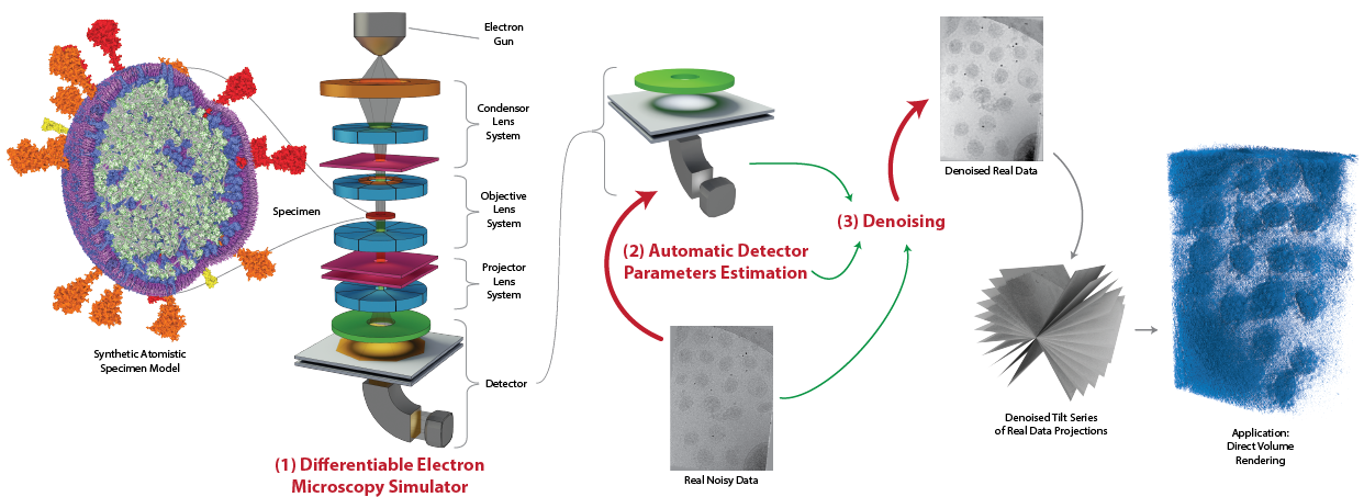
Figure 1: Three main contributions of this work are: (1) DiffTEM: a differentiable electron microscopy simulator, (2) a use case for automatic detector parameter estimation, and (3) a use case for denoising the data from real electron microscope.

Keywords Transmission Electron Microscopy Simulation; Data Models; Software Prototype; Life Sciences, Health, Medicine, Biology, Bioinformatics, Genomics; Computer Graphics Techniques; Image and Signal Processing

1 Introduction

With the revolution in the resolution [1] in 2014, the cryogenic electron microscopy (cryo-EM) became an unique tool to study and visualize the cell and its inner structures at the molecular level [2]. Still, extraction of the valuable information from the data obtained using cryo-EM and developing the computational methods for processing, analyzing, and/or visualizing such data are not trivial tasks. The main reason is the fact that the data acquisition process is time-consuming, costly, and is still performed mainly by bio-experts. This situation results in a relatively small amount of data available for developing learning-centric computational methods. Additionally, due to the limitation to only use low electron beam doses to protect the specimen, the data always suffer from a low signal-to-noise ratio (SNR). Finally, because of the limited specimen tilting during the acquisition process, high-tilt projections are missing, which results in the missing wedge problem [3]. All these shortcomings make the usage of such data difficult for visualization. To overcome these challenges, it is possible to use highly-accurate simulated data, which are similar-to-indistinguishable to the actual acquired data. Such simulation data can be easily used in ground-truth based evaluations, since the input structural model is known prior to the microscopy simulation process. It can be used in training structural biologists to learn interpreting microscopy projections, i. e., micrographs. Such simulation can be also regarded as a distinct rendering style, useful for example in generating animation sequences where a biological structure is transformed into a micrograph and vice versa. Last but not least, such data can be used for developing new Deep Learning (DL) methods for interpreting real micrographs, their testing, evaluation, and validation.

In recent years, researchers have developed several TEM simulators to support studies in biological specimen research, some of which are based on physical principles  [4, 5, 6] or parallel multi-slice simulation [7]. The simulator presented by Rullgård et al. [4] uses the multi-slice method [8] for modeling the interaction of electron and biological specimen, which is well suited for a computer simulation [9]. Additionally, the authors have developed a phantom generator for generating a specimen model and the calculation of its scattering potential based on a physical model. The above-mentioned simulator properties make it a good choice for simulating an acquisition process of biological specimens using cryo-EM. However, the simulator has two major limitations. First, the simulated microscope parameters need to be calibrated manually, which is a tedious and time-consuming process where even the initial values are not available. Second, the simulator is very slow when simulating structures larger than a few proteins. Some enveloped viral particles are huge macromolecular model (e. g., ZIKA or SARS-CoV-2). It is entirely infeasible to run a microscopy simulation of many instances of such particles with any of the previous microscopy simulation systems.

In the field of differentiable rendering, visualization problems are addressed with the use of differentiable pipelines. For example, DiffDVR [10] uses a differentiable direct volume rendering (DVR) pipeline to optimize view points, transfer functions and voxel properties. Therefore, taking inspiration from differentiable rendering, we present a fast differentiable simulator, which enables us to optimize for all continuous parameters of a microscope simulator. We demonstrate the capabilities of our differentiable simulator with two use cases, which are (1) detector parameters estimation from real data and (2) denoising. We show that using the detector parameters estimated from real data with our differentiable simulator yields accurate results. Additionally, denoising real micrographs using our pipeline is effective and outperforms state-of-the-art DL-based approaches.

This paper presents several technical contributions that and visualization applications:

• The overall architecture of the first differentiable microscopy simulator that is scalable to render realistic microscopy simulations within seconds or minutes.

• Learning detector parameters from real projections, to generate synthetic micrographs with the same detector characteristics that lead to similar visual appearance of the synthetic and the real projection.

• Utilization of deterministic and stochastic differentiation for various stages of the microscopy pipeline.

• Generation of large micrographs on par with physical dimensions and complexity of real-world microscopy.

• A new denoising method which learns from noisy projections to create a noise-free version of real-world projections. Subsequent tomographic reconstruction then results in a noise-free volume that can be used for 3D visualization.

2 Related work

First we give a brief overview of TEM simulators developed in recent years. Next, we discuss differentiable rendering and how it relates to the TEM simulation. Then, we provide background information for gradient estimation in distribution learning. Finally, we discuss related works on DL-based denoising.

TEM Simulators:

Several Electron Microscopy (EM) simulators were developed for simulating the specimen acquisition process from different domains as presented in a book by Kirkland [9]. One of the most commonly used simulators for non-crystalline biological specimens is TEM simulator presented by Rullgård et al. [4], which is also the basis for our differentiable version of the TEM simulator. The presented simulator aims to provide an accurate simulation based on a well-defined physical model. Still, the implementation of the simulator introduces a set of user-adjustable parameters (e. g., detector parameters), which require a time-consuming manual calibration process. The researchers have later presented a new TEM simulator which aims to improve the above one. While the original TEM simulator calculates the scattering potential of the specimen by estimating the potential of the atoms, InSilico TEM [5] calculates it more precisely by also including the scattering potential of molecular bonds. It also reduces the number of detector parameters and estimates them from experiments. In the recent work of Himes and Grigorieff [6], they considered the TEM simulation of amorphous samples which are sensitive to electron radiations. Additionally, they also slice the simulation in the time domain, which leads to the generation of movie frames of an exposure. The latter approaches are more accurate than the original TEM simulator [4] trading in additional physical aspects of the simulator with much higher computational costs. Nevertheless, all the presented simulators only support the forward simulation. To the best of our knowledge, our proposed work is the first to offer a forward and backward approach to simulation through differentiability, which is crucial in optimization for different visualization tasks.

To solve the reconstruction problem, CryoGAN [11] takes advantage of a Generative Adversarial Network (GAN) [12] and uses an EM simulator based on the ASTRA Toolbox [13] for generating realistic EM projections. During the forward calculation, it utilizes the simulation algorithm from the toolbox, while the back-projection approach from the toolbox is used to calculate gradients to enable differentiability. Given a training dataset of noisy micrographs, researchers crop empty patches that contain only background noise from the data. Next, they train a neural volume generator, whose generated volumes are fed into the simulator from the toolbox to generate clean micrographs. The empty patches of background noise are added to the clean micrographs, mocking noisy micrographs. The resulting noisy micrographs are given to the discriminator network, along with the real noisy micrographs. In contrast to our approach, this method does not model noise generation within the simulation and therefore assumes that the noise in micrographs is signal-independent. However, in the physical model of the TEM simulator [4], this assumption does not hold because the models for shot noise and detector blurring depend on pixel values. Moreover, CryoGAN [11] assumes that the background noise is similar throughout the specimen, which is not the case due to the change in thickness of the specimen from center towards the boundary.

Differentiable Rendering:

Together with neural rendering, it has seen dramatic progress mostly in the context of computer vision and photorealistic rendering. For example, in Li et al. [14], rendering parameters (e. g., scene geometries, camera intrinsics, and lighting conditions) can be estimated directly from images thanks to its differentiability. Hasselgren et al. [15] use a gradient estimator to optimize for ray tracing rendering parameters (i. e., sample numbers of pixels). MVTN [16] takes advantage of a differentiable renderer to optimize for the performance of a downstream task (i. e., 3D geometry classification).

If we compare photorealistic rendering with TEM simulation in a general sense, they both share similar pipelines from geometries to rendered artifacts, given a rendering method. Similar to how differentiable rendering has opened a new view on solving well-known problems in a novel way with an explainable approach, can differentiable EM simulation provide new insight into solving simulation-related problems with an optimization approach. CryoGAN [11] already shows promising results along these lines. The main difference is that it was developed for a single-particle reconstruction and is thus lacking generalizability. In the recent work, Kniesel et al. [17] developed a differentiable Scanning Transmission Electron Microscopy (STEM) pipeline and showed promising results for implicit volume reconstruction. With our TEM simulator, we can estimate Modulation Transfer Function (MTF) parameters of the simulator’s detector part, which is in a way similar to estimating rendering parameters in a differentiable rendering method as was shown by Weiss and Westermann [10] for direct volume rendering. Moreover, our approach provides a novel approach for denoising by using images generated with a TEM simulator in a similar way as Noise2Noise [18] and Topaz-Denoise [19] but based on a simulator physics model [4].

Gradient Estimation in Distribution Learning:

Distribution learning has been a challenging problem in various fields of DL. There are many approaches to learning a random distribution. Still, they can be classified into two categories, learning the parameters of distributions (e. g., $\mu$ and $\sigma$ of a normal distribution) and learning the manipulation of distributions, (e. g., $f_{\theta}(x)$ where $\theta$ parameterizes $f$, and $x$ is sampled from a prescribed distribution).

In some scenarios, the distribution of the learning objectives of a task is not known. For example, in face generation, the distribution of faces is not known nor well-defined, which means random distributions must be prescribed and manipulated. Therefore, how to manipulate predefined random distributions is the key target of optimization. Formally, such learning can be formulated as

$$\underset{\theta}{\operatorname*{\arg\min}}\ \mathbb{E}(L(f_{\theta}(X),Y)),\ X\sim D,$$

where $\theta$ is the set of parameters of $f$, $L$ a loss function, $D$ a prescribed distribution, and $Y$ a training dataset. GAN [12] is a typical case in which the optimization targets are not the parameters of the prescribed distributions but the parameters of the functions that manipulate the distributions.

When the distribution of the learning objectives is known, the distribution parameters are often the optimization target. For example, in Reinforcement Learning (RL), models can be asked to make stochastic decisions with a discrete distribution (e. g., a categorical distribution). In such settings, the optimization can be described formally as:

$$\underset{\omega}{\operatorname*{\arg\min}}\ \mathbb{E}(L(f(X),Y)),\ X\sim R(\omega),$$

where $\omega$ is the set of parameters of a distribution $R$. From the perspective of Calculus, $\frac{\partial L}{\partial\omega}$ is not defined, so researchers turn to statistical gradient estimators. One of the most widely used gradient estimators is the Monte Carlo (MC) family. The details of MC gradient estimators are beyond the scope of this paper, so we refer the reader to the review on MC gradient estimators [20].

Variational Autoencoder (VAE) [21] is a hybrid case in which distributions’ parameters and functions’ parameters that manipulate the distributions are jointly learned. VAE can be formulated as:

$$\underset{\{\theta_{0},\theta_{1}\}}{\operatorname*{\arg\min}}\ \mathbb{E}(L(g_{\theta_{1}}(Z),Y)),\ Z\sim P(f_{\theta_{0}}(X)),$$

where $f$ and $g$ are functions paremterized by $\theta_{0}$ and $\theta_{1}$ respectively and $P$ a distribution of a prescribed type parameterized by $f_{\theta_{0}}(X)$.

As new and even more complex probabilistic models than VAE emerge, existing gradient estimators and optimization techniques that are designed for specific models are not enough for training new models. Therefore, Schulman et al. [22] seek a general formulation of probabilistic models, which is stochastic compute graphs. Based on stochastic compute graphs, they devised a new way to transform deterministic loss functions into ones whose gradients are general gradient estimators of all parameters, including parameters of distributions. Such loss functions are called surrogate loss functions, and the compute graph including surrogate loss functions is called a surrogate loss function computation graph.

In our work, when estimating detector parameters, we take a GAN-like approach, optimizing for function parameters by prescribing a distribution. In the case of denoising micrographs, we define the surrogate loss function computation graph for gradient estimation based on the work of Schulman et al. [22].

2.1 Denoising

When denoising cryo-EM micrographs, clean references are not available, so many approaches have been proposed to specifically denoise cryo-EM micrographs, addressing this problem.

Researchers have proposed various analytical filters for denoising, such as simple averaging, Gaussian filters, and many filters in the frequency space that enhance or damp signal responses. Additionally, physics-based techniques were proposed, such as Nonlinear Anisotropic Diffusion (NAD) [23], which takes advantage of a diffusion model to denoise 3D volumes. For a comprehensive review on filters used in cryo-EM, we refer the reader to the review [24].

In the era of DL, many neural networks are proposed to denoise cryo-EM micrographs. Noise2Noise [18] is a general denoising approach that does not require clean data and has been adapted in CryoCARE [25] and Topaz-Denoise [19]. In CryoCARE [25], a neural network is trained as a denoiser with multiple micrographs that come from multiple consecutive exposures or multiple aligned micrographs in a tilt series or movie frames captured during a long exposure. In Topaz-Denoise [19], the researchers trained the model with a larger dataset containing thousands of micrographs acquired in different conditions, which enables better generalizability of their neural networks. Besides Noise2Noise-based approaches, Noise-Transfer2Clean (NT2C) [26] trains two neural denoisers and a GAN-based noise synthesizer to decouple noise from micrographs that are generated using a cryo-EM simulator based on real and synthetic data.

The implicit reconstruction approach by Kniesel et al. [17] also incorporates a normalizing flows neural network to model the noise distribution in the STEM data in a signal-dependent manner, allowing them to separate the noise from the clean reconstruction.

Our approach is similar to Noise2Noise [18] in the way that our model is required to output similar noisy images (i.e., noisy EM projections). However, in our simulator, we do not involve neural networks but a physical model.

3 Architecture overview

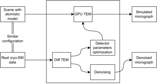
Figure 2: Our GPU-TEM simulator receives scene configuration and detector parameters estimated from real data by Diff-TEM simulator for generating simulated micrograph. Our Diff-TEM simulator denoises the real data, the denoised data can be used for reconstruction and the reconstrution can be visualized by direct volume rendering.

Our system contains two simulators as shown in Figure 2, GPU-TEM for rendering and Diff-TEM for learning. The GPU-TEM receives the scene with the same configuration as used for acquisition with the real cryo-EM, and the learned parameters (e. g., MTF) from the Diff-TEM as inputs. It then simulates the synthetic data that are similar to the real data. The Diff-TEM receives the real cryo-EM data and performs the learning, e. g., estimating MTF parameters or denoising the real data. By using this design, our system resolves two limitations of the TEM Simulator [4]: (1) the need for user-estimated parameters, and (2) a time-consuming simulation process for scenes containing many instances of macro-molecular structures.

Both the GPU-TEM and the Diff-TEM simulators are based on the TEM simulator [4] and its main purpose is to simulate the image formation process. The simulator contains components similar to a real microscopy system: electron gun; specimen; optical system – aperture, condenser lens, objective lens, projector lens, and detector. The schema of the simulator is shown in Fig. 3, where we specify the parameters with their names in blue boxes, the outputs of a step in green boxes, and stochastic nodes in circles.

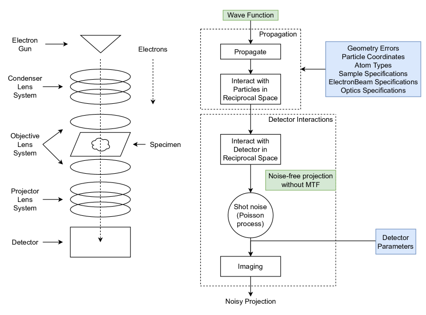
Figure 3: TEM simulator contains an electron guns, optical system with many lens, a detector and a specimen. Each electron is defined by its wave function, it interacts with specimen give the scattered wave function which is recorded at detectors to form micrographs.

To simulate the image formation process, the simulator performs two tasks. First, assembling a model of the specimen and calculating the scattering potential of the specimen are completed by the phantom generator. Second, simulating the image formation process is further split into electron-specimen interaction, electron wave propagation, and intensity detection by the detectors.

The phantom generator allows to define a specimen, including objects, background, and distribution of objects within the background. The background is assumed to be pure cryonized water. The phantom generator receives as input an atomistic model of objects defined by homologous proteins from Protein Data Bank (PDB) [27], their distribution within the specimen (user-defined or random), sample properties (thickness, sample hole diameter), and electron gun voltage. From the inputs, it calculates the scattering potential of objects by summing the electrostatic potential of individual atoms. Next, it calculates the scattering potential of the background. Finally, it fuses background and object potentials. The details of the calculation are presented in Appendix B of the TEM simulator paper [4].

Electron-specimen interaction is modeled using the Helmholtz equation presented in the work of Fanelli and Öktem [28]. Electron wave propagation through the specimen is modeled using the multi-slice method [8] that accounts for the thickness of the specimen and multiple scattering. The method divides the specimen into many slices with suitable thickness and describes a single electron with its wave function. For each slice, the electron wave interacts with the atoms of objects (particles) within the slice, followed by the transmission and propagation to the next slice. The process continues until the electron wave leaves the specimen.

The optical system is modeled as a convolution operator on the scattered electron wave. After leaving the specimen, the electron wave is subject to defocus, spherical aberration, and chromatic aberration of electron microscope lens. These effects are modeled through the optics contrast transfer function.

After passing the electron microscope lens, a scattered electron wave is detected by the detector. The detector is defined as a rectangular area of square pixels and characterized by parameters such as gain, MTF, detective quantum efficiency, and noise sources. The primary type of noise is the shot noise [29] due to fluctuations in the number of electrons which are emitted within a given time from the electron source and detected at each pixel. The electron detection in one pixel is independent with other pixels. Therefore, it is reasonably modeled with the Poisson distribution taking the pixel intensity as the expected value. In this work, we adapted the detector in line with the direct detector so other types of noise can be eliminated [30]. The detective quantum efficiency describes the detector response of the signal. The MTF describes the resolution of the detector and is defined by the modulus of the Fourier transform of Point spread function (PSF). The PSF specifies the blurring of each electron contribution when detected at a pixel and propagates it into the neighboring pixels. The PSF is a real-valued even function, so MTF is real valued as well. The assumption used in the TEM simulator [4] is that PSF is rotationally symmetric, so we can define MTF as the Fourier transform of PSF.

The MTF is commonly parametrized [31] as:

$$\operatorname{MTF}(\omega)=\frac{a}{1+\alpha\omega^{2}}+\frac{b}{1+\beta\omega^{2}}+c,$$ (1)

where $\omega$ is the spatial frequency in unit of 1/pixel. $a$, $b$, $c$, $\alpha>0$, and $\beta>0$ are the parameters depending on the type of detector and independent of the specimen.

4 TEM Implementation

To accelerate the TEM simulator, we developed the GPU-TEM simulator that exploits parallelism of the GPU hardware using the CUDA API [32]. A large portion of the simulator pipeline is implemented in CUDA, while there are some stages where we resort to the CPU implementation. We make a parallel version of the phantom generator and a per-slice parallelized version the electron-particle interaction algorithm.

For the phantom generator, the most time-consuming task is computing the scattering potential of biological structures (particles). The scattering potential of one particle is calculated by the sum of the scattering potential of all atoms that form the particle. In the original TEM [4] simulator, this task is performed sequentially. To overcome this bottleneck in our GPU-TEM, we make a CUDA kernel for computing scattering potential for one atom, so the scattering potential of all atoms in the particle is computed in parallel at the atom level.

To calculate the electron-specimen interaction of each slice, we first determine which structures of the specimen are within the slice. Then we calculate the scattered electron wave after it interacts with these particles. This task is also performed sequentially in the original TEM [4] simulator. We make another CUDA kernel in our GPU-TEM simulator to compute the scattered electron wave after it interacts with one structure, so the electron-specimen interaction of each slice is computed in parallel at the particle level.

To implement our Diff-TEM simulator, we use Pytorch [33] and Taichi [34, 35]. Pytorch is a well-known machine learning framework for parallel computing with GPU acceleration. With Pytorch, all gradients of each component in the simulator are calculated automatically and can be used for optimization with gradient descent. However, the TEM simulator uses the multi-slice method for computing the electron-specimen interaction, which is a sequential algorithm and hard to be expressed in Pytorch operators. Therefore, to speed up and differentiate this computation, we use Taichi [34, 35] and implement the calculation using Taichi kernels.

Our Diff-TEM simulator is differentiable, so all continuous parameters of different parts of the simulator can be optimized or learned from the real data via backpropagation and gradient descent. We demonstrate this capacity through two examples: (1) MTF parameters estimation and (2) denoising. From the pipeline, the final projection is obtained by adding Poisson noise to the noise-free projection and applying MTF afterward. Therefore, to estimate MTF, we perform backpropagation from real projections and use gradient descent for optimization. To denoise the real projections with gradient-based optimizations, we estimate the gradients of Poisson noise by using the method proposed by Schulman et al. [22] and apply gradient descent.

5 Learning components

The differentiability gives us the capability to estimate parameters along the entire electron microscopy process pipeline. In this paper we focus on detector parameters, which are at the very end of the microscopy simulation.

5.1 MTF Parameters Estimation

Because MTF parameters are independent of the specimen, we can optimize these parameters by using a few crops of background from the real projections. These crops are $M\times N$ pixels in size. They are considered as the labelled projections $I_{l_{1}},I_{l_{2}},\ldots,I_{l_{n}}$. The predicted projections $I_{p_{1}},I_{p_{2}},\ldots,I_{p_{n}}$ are created using our simulator with the same configuration for the sample, electron beam and optical system. The specimen of the predicted projection contains only the background. The predicted projections have the same size as the labelled projections. Both labelled projections and predicted projections are normalized to the range $[0,1]$. Applying MTF is performed in the frequency domain which is motivation for us to choose a loss function that can capture the differences of the predicted and the labelled projection in both spatial and frequency domain. In this work, we choose focal frequency loss (FFL) [36] combined with mean square error (MSE) by summing them into the loss function.

The computational graph for estimating the MTF parameters is shown in Fig. 4.

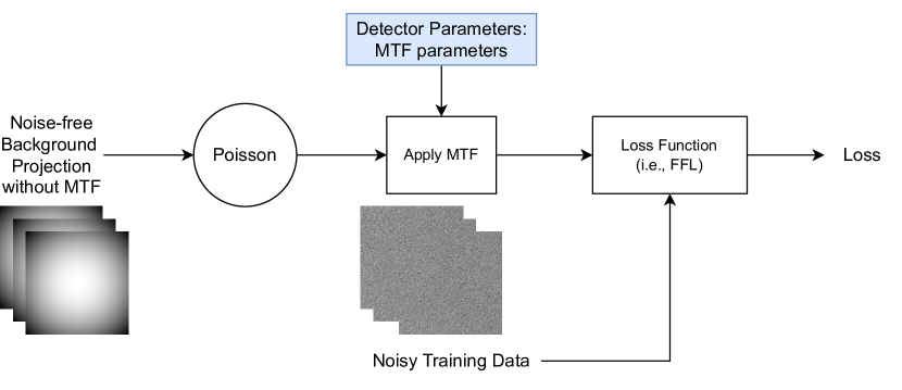
Figure 4: Compute Graph of Detector Parameter Estimation: The Diff-TEM first receives noisy training data, computes the loss with simulated noisy data, applies the predicted MTF, and performs gradient descent for optimizing MTF parameters.

The optimization can be formally described as:

$$\underset{\Theta_{D}}{\operatorname*{\arg\min}}\ \mathbb{E}(L(\operatorname{MTF}_{\Theta_{D}}(\operatorname{Poisson}(\tilde{I})),\ \operatorname{ND})),$$

where $\Theta_{D}$ is the set of MTF parameters, $\tilde{I}$ a noise-free projection without MTF, $\operatorname{ND}$ is the noisy dataset, and $L$ is the loss function. $\operatorname{ND}$ can be the synthetic or real-world data. We conducted experiments for both.

The FFL loss is defined through a weight matrix and a frequency distance matrix. $F_{l_{1}},F_{l_{2}},\ldots,F_{l_{n}}$ are 2D discrete Fourier transforms of labelled projections $I_{l_{1}},I_{l_{2}},\ldots,I_{l_{n}}$. $F_{p_{1}},F_{p_{2}},\ldots,F_{p_{n}}$ are 2D discrete Fourier transforms of predicted projections $I_{p_{1}},I_{p_{2}},\ldots,I_{p_{n}}$.

The FFL of labelled projection $I_{l_{i}}$ and predicted projection $I_{p_{i}}$ is:

$$\operatorname{FFL}(F_{l_{i}},F_{p_{i}})=\operatorname{mean}(w(F_{l_{i}},F_{p_{i}})*\left|F_{l_{i}}-F_{p_{i}}\right|^{2})$$ (2)

where $\left|F_{l_{i}}-F_{p_{i}}\right|$ is frequency distance between the labelled projection $I_{l_{i}}$ and the predicted projection $I_{p_{i}}$, $w(F_{l_{i}},F_{p_{i}})=Normalize(\left|F_{l_{i}}-F_{p_{i}}\right|^{\alpha})$ is weighted matrix, $\alpha$ is the scaling factor for flexibility. The bigger $\alpha$ is, the more focus on optimization for hard frequencies (frequency components that are hard to synthesize). We conducted an experiment with different values for $\alpha$ and chose the best one.

The MTF parameters are optimized using the Adam optimizer [37] $(\beta_{1}=0.8,\beta_{2}=0.992,lr=0.1)$. We also experimented with optimization using only MSE loss. The evaluation shows that combining FFL and MSE performs best for the task.

$I_{l_{n}}\leftarrow Noisy\ Projections$

$I_{l_{n}}\leftarrow\operatorname{Normalize}(I_{l_{n}})$

$\Theta_{D}\leftarrow random\ values$

$\tilde{I}\leftarrow noise\verb|-|free\ projection\ without\ \operatorname{MTF}$

$\alpha\leftarrow Learning\ Rate$

$IT\leftarrow\ iterations$

$i\leftarrow 1$

while $i\leq IT$ do

     $I_{p_{n}}\leftarrow\operatorname{MTF}(\operatorname{Poisson}(\tilde{I}))$

     $I_{p_{n}}\leftarrow\leftarrow\operatorname{Normalize}(I_{p_{n}})$

     $loss\leftarrow\operatorname{MSE}(I_{p_{n}},I_{l_{n}})+\operatorname{FFL}(I_{p_{n}},I_{l_{n}})$

     $\Theta_{D}\leftarrow\Theta_{D}-\alpha\frac{\partial loss}{\partial\Theta_{D}}$

     $i\leftarrow i+1$

end while

return $\Theta_{D}$

Algorithm 1 MTF Parameters Optimization

5.2 Denoising

As shown in Fig. 3, in the forward computation of our simulator, the input of quantization is a noise-free projection without MTF and the output of our simulator is a noisy projection.

Since our simulator is differentiable, we can do inverse computations via gradient descent, which means we can re-formulate the problem of denoising into an inverse problem. That is, given noisy data and a differentiable compute pipeline, to recover the noise-free projections without MTF, which are in the upstream of our forward computation. The optimization can be formulated as:

$$\underset{\tilde{I}}{\operatorname*{\arg\min}}\ \mathbb{E}(\operatorname{SL}(\operatorname{MTF}(Q(\tilde{I})),\ \operatorname{RD})),$$

where $\tilde{I}$ is the recovered denoised projection without MTF, $\operatorname{SL}$ the surrogate loss function devised from the work of stochastic compute graph [22], $\operatorname{RD}$ the real data (e. g., noisy SARS-CoV-2 projections), and $L$ a loss function. To get a denoised projection $I_{d}$ from $\tilde{I}$, we bypass the quantization and apply MTF directly, which means $I_{d}=\operatorname{MTF}(\tilde{I})$.

The compute flow of the optimization of denoising is shown in Fig. 5. The $\tilde{I}$ (i. e., Projection without MTF) is initialized with random values. The quantization models the shot noise of a detector. Given a Poisson distribution and its parameter $\lambda$, we can calculate the log likelihood of a sampled value $x\sim\operatorname{Poisson}(\lambda)$, which is denoted as $\operatorname{LL}(x,\lambda)=ln(P(x|\operatorname{Poisson},\lambda))$ where $ln$ is the natural logarithm. After sampling with quantization and calculating log likelihoods, the results with shot noise $I_{q}$ (i. e.Noisy Projection without MTF in Fig. 5) are applied with MTF, which yields the predicted noisy projections $I_{n}$.

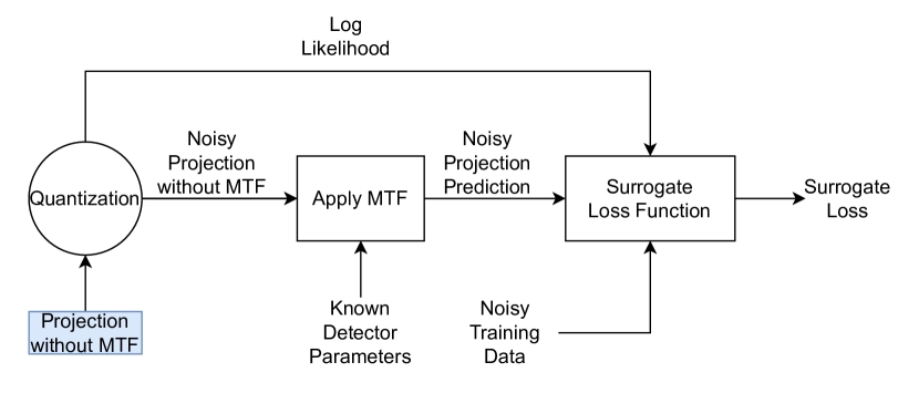
Figure 5: Compute graph of denoising: The projection without MTF is the optimization target. Log likelihood values are used in our surrogate loss function along with the comparison loss that computes the difference between noisy projection predictions and noisy projections in a dataset.

Inspired by the surrogate loss functions by Schulman et al. [22], we take the surrogate loss function as Eq. 3 where $\operatorname{ll}$ equals $\operatorname{LL}(I_{q},\tilde{I})$ and $\operatorname{mean}(\cdot)$ is the operator taking the mean value of all values in a tensor.

$$\operatorname{SL}(I_{n},\operatorname{RD},\operatorname{ll})=\operatorname{mean}((\operatorname{RD}-I_{n})^{2}*\operatorname{ll}).$$ (3)

The whole optimization algorithm is shown in Algorithm 2. The normalization trick in Line 5 ensures consistent and standardized contrast and thus stabilizes our optimization. Note that due to the scarcity of real noisy projections, we perform data augmentations to generate meaningful training data. For one micrograph $P$ in a tilt series, we align its neighboring micrographs, which are denoted as $P_{-}$ and $P_{+}$, using perspective-based image alignment in OpenCV [38] because we assume that neighboring micrographs have minor differences compared to $P$, which is a reasonable assumption when the tilt angle increment is small, for example, 2-3 degrees. Therefore, in Algorithm 2, $P_{n}=\{P_{-},P,P_{+}\}$. Furthermore, we preprocess $P_{n}$ with Topaz-Denoise [19] to generate training data that are less noisy. The data augmentation is optional in the synthetic setting because we have sufficient amount of noisy training data, but in the real setting, it is necessary because (1) the available raw data is scarce (i. e., only one), (2) the amount of information from only one projection with a low SNR is limited, and (3) as discussed in Section 2.1, our method is essentially a physical-model-based Noise2Noise [18], which means it cannot be trained with only one projection. In the denoising optimization, we use Adam [37] as the optimizer with $(\beta_{1}=0.8,\beta_{2}=0.992,lr=1.0)$.

1:$P_{n}\leftarrow Noisy\ Aligned\ Projections$

2:$\alpha\leftarrow Learning\ Rate$

3:$IT\leftarrow\ iterations$

4:$P_{t}\leftarrow\operatorname{Topaz-Denoise}(P_{n})$

5:$P\leftarrow\operatorname{Normalize}(P_{n}\cup P_{t})$

6:$\tilde{I}\leftarrow random\ values$

7:$i\leftarrow 1$

8:while $i\leq IT$ do

9:     $I_{q}\leftarrow Q(\tilde{I})$

10:     $\operatorname{ll}\leftarrow\operatorname{LL}(I_{q},\tilde{I})$

11:     $I_{n}\leftarrow\operatorname{MTF}(I_{q})$

12:     $\operatorname{loss}\leftarrow\operatorname{SL}(I_{n},P,ll)$

13:     $\tilde{I}\leftarrow\tilde{I}-\alpha\frac{\partial\operatorname{loss}}{\partial\tilde{I}}$

14:     $i\leftarrow i+1$

15:end while

16:$I_{d}=\operatorname{MTF}(\tilde{I})$

Algorithm 2 Denoising Optimization

6 Reverse-Engineering MTF

For estimating MTF parameters, we perform experiments on both synthetic and real-world data. The synthetic data is created from the envelope of SARS-CoV-2 and Tobacco Mosaic virus (TMV) virions. The real-world dataset is provided by Yao et al. [39] and consists of 20 tilt series containing several SARS-CoV-2 virions each. For the purpose of parameter optimization we only use cropped sub-projections containing background. The real data was acquired using a Titan Krios microscope with K3 detector from Gatan, operated at a voltage of $300$ kV. The ground truth of MTF parameters for real data was obtained by performing curve-fitting from MTF curve of Gatan K3 detector. The ground truth values of MTF parameters for the synthetic data TMV are provided by Rullgård et al. [4] in their simulation and calibrated with their real data which is the micrograph of TMV virions measured by a Philips CM 200 FEG TEM microscope.

We conducted experiments for each loss function (MSE, MSE + FFL) with varying number of background images of synthetic data to see the correlation between performance of each loss and the numbers of projections. The number that gives the best performance on synthetic data is used for the number of projections we use in experiments with real data. Furthermore, we conducted experiments with varying FFL loss $\alpha$ values: $(0.0,0.5,1.0,2.0)$. To demonstrate the generalization of the estimation method, we also experimented with synthetic data using MTF varying in shape from the previous MTF used in synthetic and real data cases.

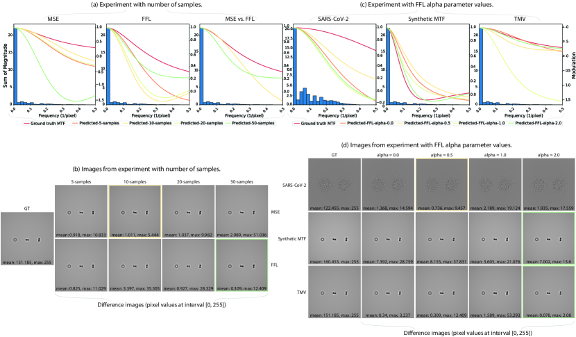
Figure 6: MTF parameter estimation experiment results: (a) Predicted MTF curves estimated by using MSE and FFL with different number of sample; (b) Noise-free projections applied MTF s in (a); (c) Predicted MTF curve for each scene using different $\alpha$ value for FFL; (d) Noise-free projection of each scene when applying MTF s in (c).

The effect of MTF is difficult to visually inspect in the noisy cryo-EM projections because of low SNR. Therefore we applied both ground truth MTF and predicted MTF on the noise-free projection of the synthetic scene for evaluation. The details of the synthetic data, the number of background projections, and ground truth values of MTF parameters $(a,b,c,\alpha,\beta)$ are shown in Table 1.

Table 1: Details of experiments for estimating MTF parameters

Subject	MTF paramters	No. of images
3 TMV	0.7, 0.2, 0.1, 10, 40	5, 10, 20, 50
$\approx 10$ SARS-CoV-2	0.6, 1.24, -0.84, 0.97, 0.97	48
TMV with synthetic MTF	-2.86, 2.113, -0.1318, 57.288, 25.429	50

To evaluate the effect of the MTF on the noise-free projection, we calculated the contribution of each frequency for the noise-free projection and determined which frequency band yields the largest contribution by summing the magnitude for each band. The frequency bands (in units $\frac{1}{pixel}$) we used are $\left\{[0.0,0.02),[0.02,0.04),\ldots,[0.48,0.5)\right\}$. If the predicted MTF aligns well with the most contributing frequency bands of the ground truth MTF, their effects on the noise-free projections are similar. Additionally, from the noise-free projections that applied ground truth MTF and predicted MTF, we first calculate pixel-wise difference between them, then compute the mean and maximum of the pixel-wise difference. If two MTF s align with the ground truth MTF in the same degree, the better one is the MTF which has the smaller mean and maximum difference values.

The correlation between the number of background projections and the performance of each loss function on synthetic data is shown in Fig. 6 (a, b). The MSE performance decreases when the number of background projections is greater than 10, the gap between the predicted MTF and the ground truth MTF increases, the mean and maximum differences also increase. With 50 background projections, the projections with applied predicted MTF are blurry, and it is hard to see the details of individual TMV virions. On the contrary, FFL performance improves when increasing the number of background projections. The predicted MTF with 5 background projections is more aligned with the ground truth MTF than 10, 20 background projections. However, the estimation from 50 background projections is better. The projection applied with the predicted MTF based on 50 projections has the smallest mean and maximum differences values. The comparison of the best MSE and FFL results is shown in Fig. 6 (a, b). It is clear that FFL is a better choice than MSE.

We also investigated how the change of FFL $\alpha$ parameter affects the MTF estimation for different setting. The results are shown in Fig. 6 (c, d). The best predicted MTF for SARS-CoV-2, TMV, and synthetic setting are obtained by using $\alpha=0.5$, $\alpha=2.0$, $\alpha=2.0$, for FFL respectively. The best $\alpha$ value for each experiment is different because of the settings (electron dose, sample preparation, etc.) of different experiments are not the same, the distribution of frequencies in background projections is different. The results show that our system works effectively for different types of MTF curve. The first type is the real MTF (TMV and SARS-CoV-2), which gives high modulation in the most contributing frequency bands. This results in preservation of virion details. The second type is the synthetic MTF, the modulation decreases in the most contributing frequency band, resulting in blurred images with applied MTF. Our predicted MTF for each case is aligned well with the ground truth in the most contributing frequency band, and produces similar effect on the noise-free projection.

7 Scalable TEM Simulation

Once we obtain the MTF parameters we can generate synthetic micrographs with the same detector properties as were used for a reference real micrograph. For the purpose of fast rendering we use the GPU-TEM implementation with several stages parallelized using CUDA. We compare the performance of the original TEM simulator and our GPU-TEM. In the phantom generator we used the model of SARS-CoV-2 virus modelled by Nguyen et al. [40], ZIKA virus PDB id 5IRE, and TMV PDBid 2OM3. We demonstrate the scalability of our GPU-TEM in two aspects: (1) number of atoms and (2) number of virion instances. The performance of each simulator for a single instance of each virus type is shown in Table 2. All performance experiments were done on the same workstation with one processor Intel(R) Xeon(R) CPU E5-2687W v4 3GHz and one GPU NVIDIA GeForece RTX 3090.

Table 2: Performance evaluation using varying viral models in terms of number of atoms and their rendering times using original simulator and GPU-TEM

Virions	No. of atoms	TEM [4]	GPU-TEM (Ours)
TMV	12505	45s	4s
ZIKA	21149	1m 51s	1m 46s
SARS-CoV-2	$\approx 13$ millions	7m 25s	6m 4s

From the Table 2, it can be seen that for a single instance of TMV, and a single instance of SARS-CoV-2 our GPU-TEM is faster than the baseline [4]. The performance for a single instance of the ZIKA virus is similar for GPU-TEM and the baseline. For better understanding of simulator performance, we measure the performance on a varying number of ZIKA virion instances. The results are shown in Table 3. Our GPU-TEM significantly outperforms the original implementation for scenes containing a high number of instances which are close to the realistic numbers of instances in the real microscopy experiments. Further parallelization of the simulator pipeline stages would result in an even larger performance gap.

Table 3: Performance on many instances of ZIKA

No. of instances	TEM [4]	GPU-TEM (Ours)
1	1m 51s	1m 46s
5	2m 9s	3m 1s
10	2m 16s	3m 10s
50	3m 34s	3m 30s
100	2m 16s	3m 48s
500	21m 17s	5m 42s
1000	35m 27s	6m 22s
5000	4h11m	18m 9s

To illustrate the capability of our GPU-TEM simulator, in Fig. 7 we also show the result of simulating a larger scene with multiple SARS-CoV-2 virions side-by-side with the real microscope image. The presented specimens are on the same level of complexity with respect to the number of atoms/particles.

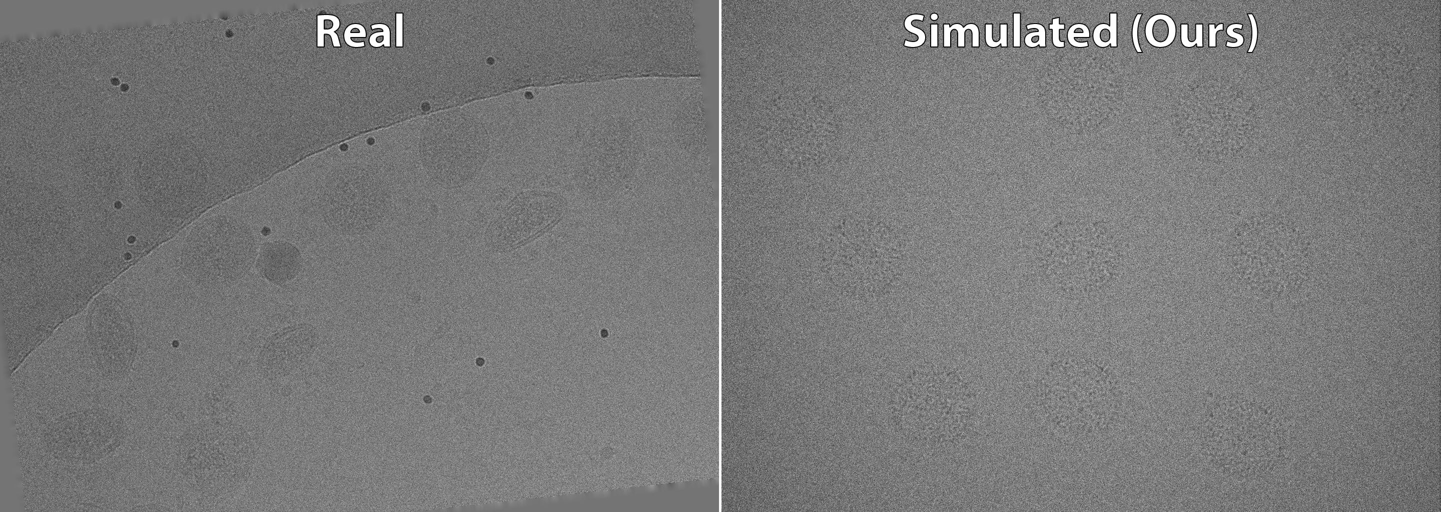
Figure 7: Real and simulated tomographs of scene with multiple SARS-CoV-2 virions.

8 Denoising Micrographs

Our differentiable simulator Diff-TEM gives us the capability to predict the noise-free version of our micrographs. We have investigated this capability by means of multiple experiments, whereby we compare the denoising capabilities of our approach in synthetic and real settings qualitatively and quantitatively.

First, we conducted experiments using a synthetic dataset generated with our simulator given TMV virions. In this setting, we obtain a clean ground truth data that is synthesized by bypassing the quantization.

Note that in simulation and in the real electron microscopy process, the dose, measured in electrons per nm² per projection, is a major factor that determines SNR. We tested our denoising method with synthetic datasets with varying doses. The higher the dose is, the higher SNR is. For generating a tilt series of 60 projections, 100 electrons/nm² per projection is a typical low dose while 2000 is a typical high dose. We tested datasets acquired using doses of {100, 200, 300, 500, 700, 1000, 1500, 2000} per nm² per projection. We used such doses because it is possible to use a very high dose (e. g., 1000) if the number of total projections is low and thus the total dose stays the same. Moreover, the number of available projections of the same scene (i. e., same tilt angle and specimen) also affects the denoising quality. We tested our method on the numbers of available projections of {2, 5, 10, 25, 50}. We denote varying data settings with pairs, i. e., (dose, number of available projections).

Moreover, to compare with the original Noise2Noise model [18] and Topaz-Denoise [19], in the synthetic setting, we trained a Noise2Noise model and a Topaz-Denoise model (denoted as Topaz T) with our synthetic data. The data setting for training the Noise2Noise model is (100, 5000) while it is (100, 4500) for training the Topaz-Denoise model. We also use the pretrained Topaz-Denoise model (denoted as Topaz P) for comparison. Note that in the synthetic setting, we do not apply any kind of data augmentation in our method.

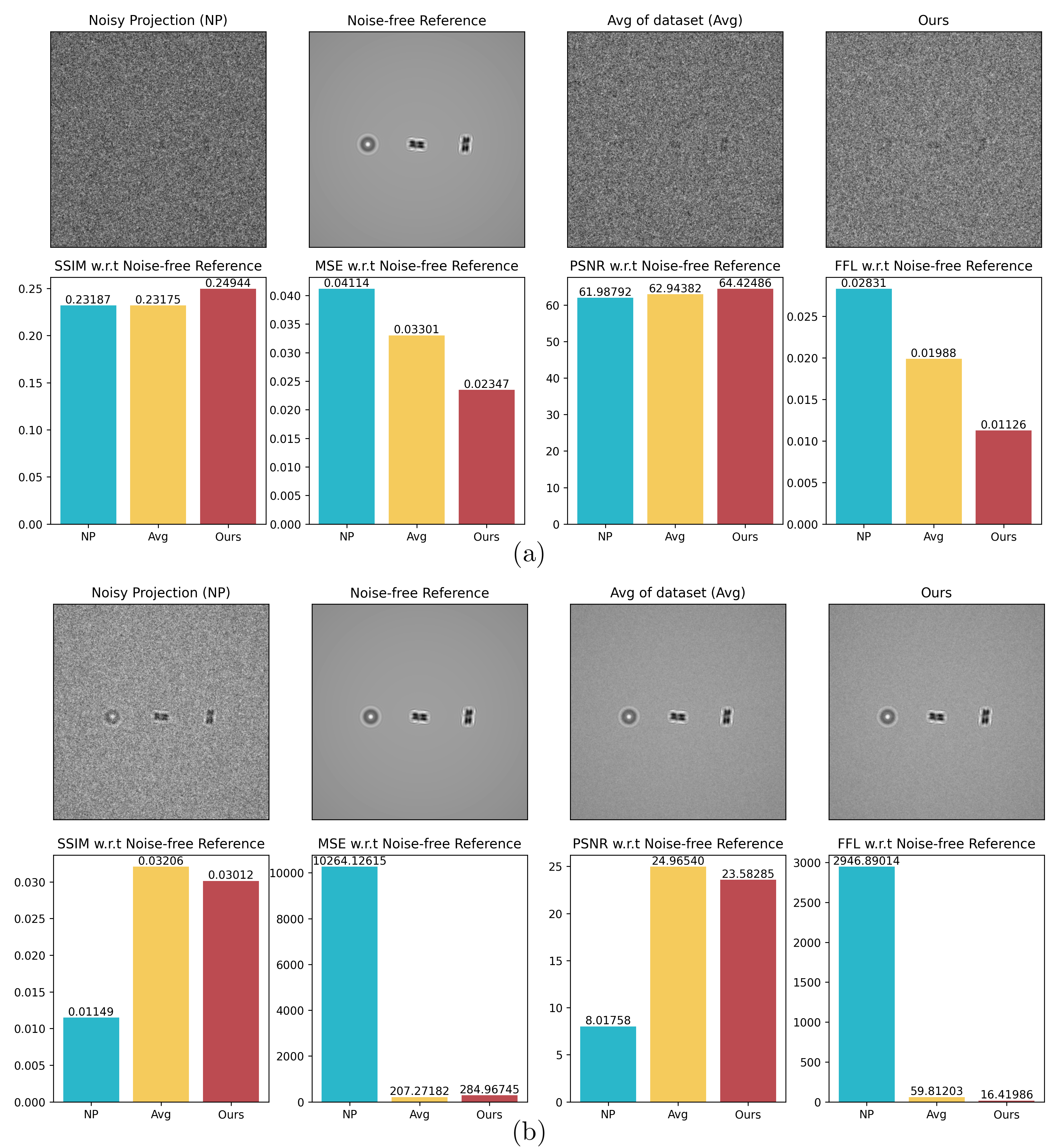
Figure 8: Denoising visual and quantitative comparison of synthetic data: (a) The results of data setting (100, 2). (b) The results of data setting (2000, 50). Note that in these two settings our method (Ours) does not apply data augmentation.

Using the synthetic data with ground truth in the setting (100, 2) shown in Fig. 8 (a), we have very limited amount of projections (i. e., only 2) and a low dose which leads to a low SNR. In settings like this where data are scarce and full of noise, a natural choice is to average the two available projections. Although the denoised result is not close to the noise-free reference, our method outperforms the simple average of the two available projections in terms of structural similarity (SSIM) [41], MSE, peak signal-to-noise ratio (PSNR) and FFL. In the very high dose cases (i. e., 700, 1000, 1500, 2000), we show consistently better results than simple averaging in terms of FFL. For example, the quantitative comparison in Fig. 8 (b) shows that the FFL of our method is roughly 4 times better than simple averaging. The quantitative comparisons of these two figures show that our physically-based Noise2Noise-like model is effective.

To compare with the original Noise2Noise [18] model and Topaz-Denoise [19], we present our results from the setting (100, 50) denoted as Ours-50 in Fig. 9. The figure also shows the results of a trained Noise2Noise model, Topaz P and Topaz T. The Noise2Noise model does not learn to denoise even if we have a large amount of available data (i. e., 5000). Therefore, we further tested the performance of the Topaz model with our synthetic dataset. The results show that the pretrained model (i. e., Topaz P) generalizes well by filtering out high-frequency noise and preserves the particles, but it is worse than our method because the boundaries of particles are blurred. Our trained Topaz model (i. e., Topaz T) filters out most of the noise and recognizes the positions of the particles. However, it does not preserve the shape of the particles, which makes it unusable. On the contrary, our method can work in the setting with less data (i. e., (100, 50)), which shows that our method is advantageous over training a Noise2Noise model [18] and a Topaz-Denoise model [19] from scratch.

It is noteworthy that the Noise2Noise model and Topaz T are trained with data settings (100, 5000) and (100, 4500) respectively. It is not realistic nor viable to obtain such large datasets in real-world scenarios, which means these two models are not usable. However, Topaz P generalizes well in our setting, so we use it for data augmentation in the real-world scenario to generate more data for our denoising method.

For more results of our method under synthetic settings, we refer the reader to the supplementary material.

Figure 9: Comparison of denoising the synthetic data: images in the top row show original noisy projection (NP) and clean ground truth projection (GT) and our denoising result, in bottom row are denoising results using the trained Noise2Noise result (Noise2Noise), pretrained Topaz-Denoise (Topaz P), and Topaz-Denoise trained on our noisy projections (Topaz T).

Table 4: SSIM, PSNR and FFL comparison

SSIM						PSNR					FFL
	Noisy	Topaz	Ours(T)	Ours(N)	Ours(T+N)	Noisy	Topaz	Ours(T)	Ours(N)	Ours(T+N)	Noisy	Topaz	Ours(T)	Ours(N)	Ours(T+N)
Noisy	1.0000	0.6017	0.4139	0.7395	0.6547	361.200	65.8250	65.8270	70.1500	66.1000	0.0000	0.0096	0.0082	0.0032	0.0095
Topaz	0.6017	1.0000	0.6894	0.7184	0.8651	65.8250	361.200	72.2000	68.9700	75.0400	0.0096	0.0000	0.0012	0.0045	0.0008
Ours(T)	0.4139	0.6894	1.0000	0.7797	0.8001	65.8270	72.2000	361.200	71.6200	76.2800	0.0082	0.0012	0.0000	0.0020	0.0001
Ours(N)	0.7395	0.7184	0.7797	1.0000	0.9098	70.1500	68.9700	71.6200	361.200	71.6700	0.0032	0.0045	0.0020	0.0000	0.0029
Ours(T+N)	0.6547	0.8651	0.8001	0.9098	1.0000	66.1000	75.0400	76.2800	71.6700	361.200	0.0095	0.0008	0.0001	0.0029	0.0000

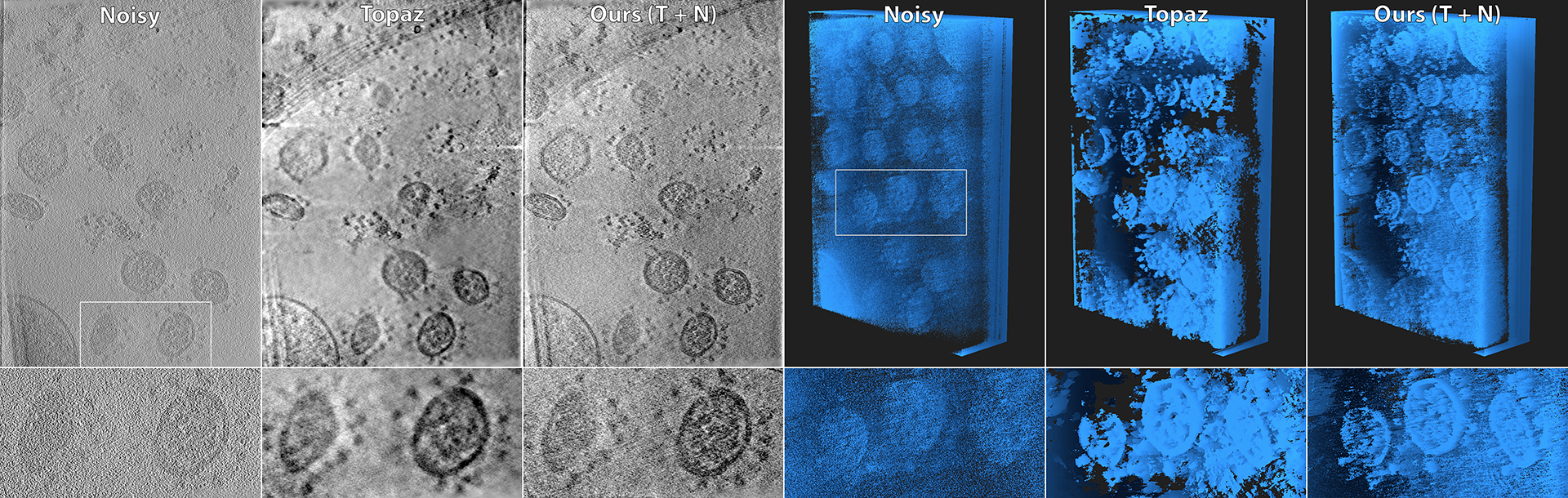
Figure 10: Tomographic reconstructions from the tilt series (left) and DVR renderings (right).

In the experiments using real micrographs, we use the tilt series from Yao et al. [39], which show SARS-CoV-2 virions. The dose in the dataset is 320 electrons per nm² per projection. Therefore, without data augmentations, the data setting is (320, 1). As discussed in Section 5.2, our method cannot work in a scenario with only single projection, so in our experiments, we apply a number of data augmentations. In the setting Ours(T), the data augmentation with Topaz P is used, yielding one more projection, which means the data setting is (320, 2). In the setting denoted as Ours(N), neighboring projections of a projection are aligned and used, so the data setting is (320, 3). In the setting Ours(T+N), Topaz P and aligned neighboring projections are used, so the data setting is (320, 6). The case of Ours(T+N) matches exactly our Algorithm 2 while in the case of Ours(T), $P_{n}=\{P\}$, and in the case of Ours(N), preprocessing with Topaz-Denoise is not used (i. e., $P_{\operatorname{train}}=\operatorname{Normalize}(P_{n})$). In the real setting, we do not have noise-free ground truth projections to compare against, so we first present results of the qualitative comparison.

On the top of Fig. 11, we can see Topaz has block-like artifacts and Noisy contains more noise while others have minor visual difference. However, if we zoom-in the images, as shown in the bottom of  Fig. 11, we can see (1) Topaz has more blurring artifacts, (2) Noisy has the most noise, and (3) Ours(T+N) is better than Ours(N) and Ours(T) in that it has less high-frequency noise while preserving clear boundaries. This makes our method Ours(T+N) the best among these five because of its good balance between denoising and preserving boundaries from the view of quality.

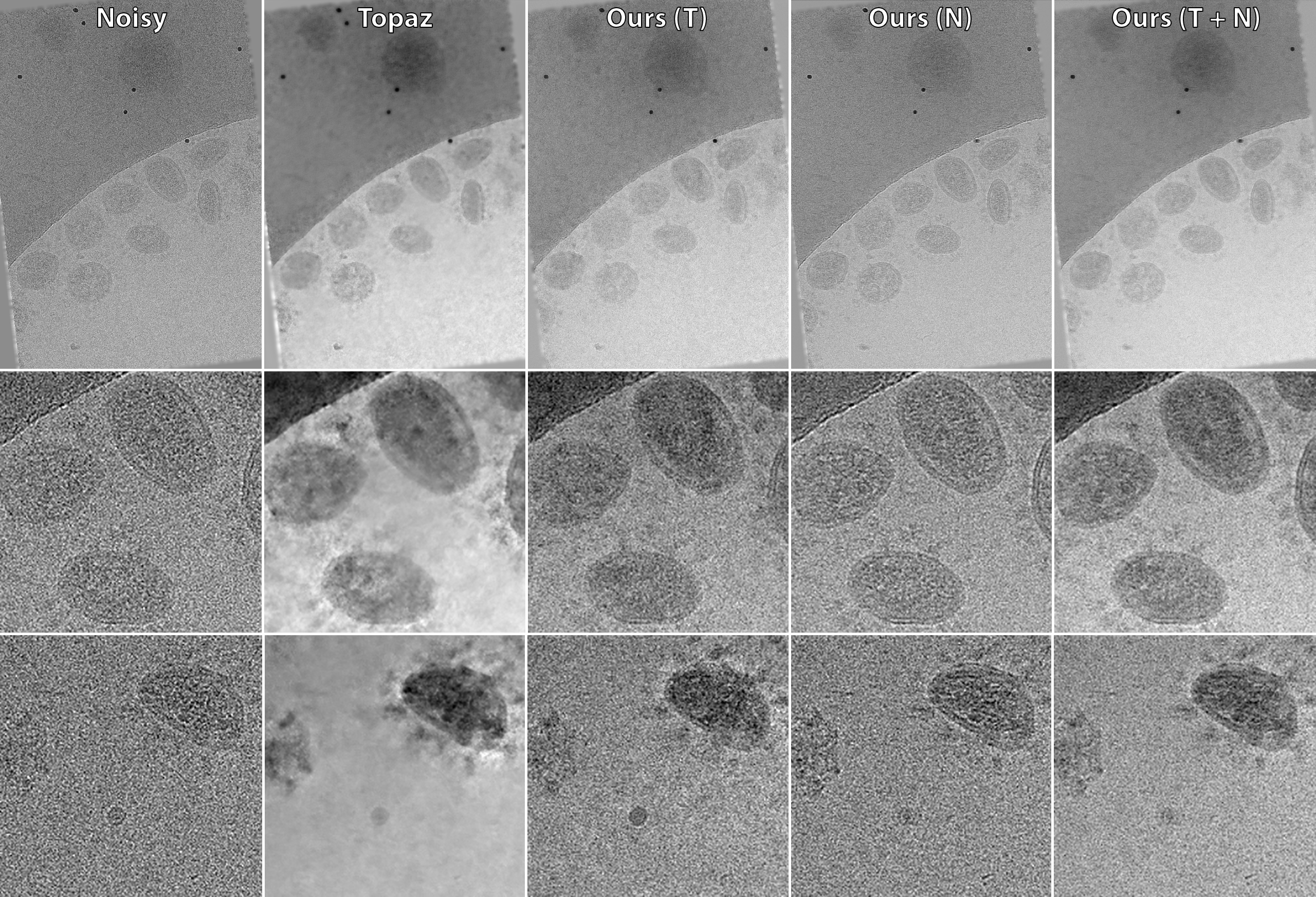
Figure 11: Topaz: the real projection denoised by Topaz P; Noisy: the real noisy projection; Top: Full views; Middle: Zoom-in of the first row. In the bottom row is another example of our denoising method, Ours(T+N) contains less noise while preserving boundaries.

We also present quantitative results in Table 4. Based on the bottom images from Fig. 11, we can conclude that Topaz contains the least noise while Noisy contains the most noise. With this conclusion, the values in bold in the table show that (1) Ours(T+N) is the closest one to Topaz and (2) Ours(T+N) has a moderate amount of noise compared to Ours(T) and Ours(N). This means Ours(T+N) is a good compromise between removing noise and preserving details, echoing with our qualitative comparison.

In addition to the example on the top two rows of Fig. 11, we give another example of denoising real data. From the last row in Fig. 11, we can draw similar conclusions. Topaz has the least noise, but compromised boundaries while Ours(T+N) has a moderate amount of noise but also clearer boundaries and more visibility of spikes.

The application of such denoising are also useful for the tomographic reconstruction. In left part of Fig. 10 we show the mid-slice from the volumes reconstructed using SIRT reconstruction technique from IMOD [42] from original noisy projections (left), from denoised projections using Topaz (middle), and from denoised projections using our approach Ours(T+N) (right). One can clearly see that Topaz and our approach are better that reconstruction from the original noisy projections. Moreover, our approach retains more details which are smudged out by Topaz.

Additionally, in the right part of Fig. 10, we show DVR rendering of the same volumes using the same rendering parameters apart from the threshold, which was manually adapted for each case. One can see that Topaz cleans the volume extensively, but also removes parts of the virions and removes the high frequency details from the structures. This is not the case for results using our approach. While there is more noise present in the volume, the high-frequency details are retained. Both approaches are clearly better choice than rendering the original noisy volume.

9 Conclusion

With this work, we have presented a system combining GPU-TEM and Diff-TEM simulators that enables rendering large micrographs on par with physical dimensions and complexity of real-world microscopy. Nonetheless, our system not only performs forward calculation, but also enables backward computation, which gives rise to a new way to solve inverse problems in microscopy imaging. We demonstrate its ability by showcasing two examples, detector parameter estimation, and denoising, which are typical inverse problems.

Our GPU-TEM simulator outperforms the baseline TEM simulator when simulating a scene containing a high number of complex structures. However, because the calculation for all slices of the specimen is still performed on the CPU, our GPU-TEM still takes time to transfer the data from GPU to CPU for this calculation. In the future, we plan to perform this calculation in parallel.

Our method for detector parameters estimation learns from the real data, automating the time-consuming manual calibration. Moreover, users can use this functionality to guess a reasonable set of parameters and fine-tune them manually if desired. This narrows the search space and speeds up tuning. However, some hyperparameters, such as $\alpha$ for FFL and the initial values for detector parameters, are selected randomly. In the future, we plan to develop a method for determining the distribution of frequencies. We can guess which frequency components are hard to synthesize, and choose a good $\alpha$ for FFL from the distribution of frequencies. We also plan to apply a DL-based approach to find a good initialization for detector parameters.

Our method of denoising is a physically-based Noise2Noise model, showing better results on our synthetic datasets than existing DL-based methods. On a real micrograph, with data augmentation using a state-of-the-art denoiser and neighboring projections, we show improvements compared to the state-of-the-art. For downstream applications, our denoised projections can contribute to better tomographic reconstruction and thus improve the quality of visualizations (e. g., DVR). In spite of the improvements, our denoising method shares the same limitation as in the original Noise2Noise [18]. This means that our method needs multiple projections to denoise one projection while in real-world scenario the data are limited. To mitigate this limitation, we believe it is possible to use neural networks to learn and transfer the patterns from various data. With the differentiability of our simulator, future work can be done to embed a neural network into the physics model of our simulator, taking advantage of the generalizability of neural networks while preserving physical intuitions.

Supplementary Material

More Comparisons of Denoising Synthetic Projections

Here we present more comparisons of results of different synthetic settings to show the effectiveness and usefulness of our denoising method.

When the number of samples is small, for example, 2 or 5. Our results are close to the averages of the datasets visually. Yet, our results are better in terms of quantitative metrics as shown in Fig. 12 and Fig. 13 in which the results of data settings of (200, 2) and (200, 5) are presented.

When the dose is high (i. e., greater than 700 electrons per nm² per projection), our method consistently outperforms the averages of the datasets by a large margin in terms of FFL, which indicates our denoising method is much more correct in frequency domain. Here we present the results of the settings (700, 10) and (1500, 10). In Fig. 14 we can see the FFL is almost 50% better than the average of the dataset and in Fig. 15 the margin is more than 400%.

Along with the results in Fig. 8, we can conclude that despite the margins are different with different data settings, our method is advantageous over simple averaging consistently. This is especially beneficial when the data are too scarce and too noisy to train neural networks.

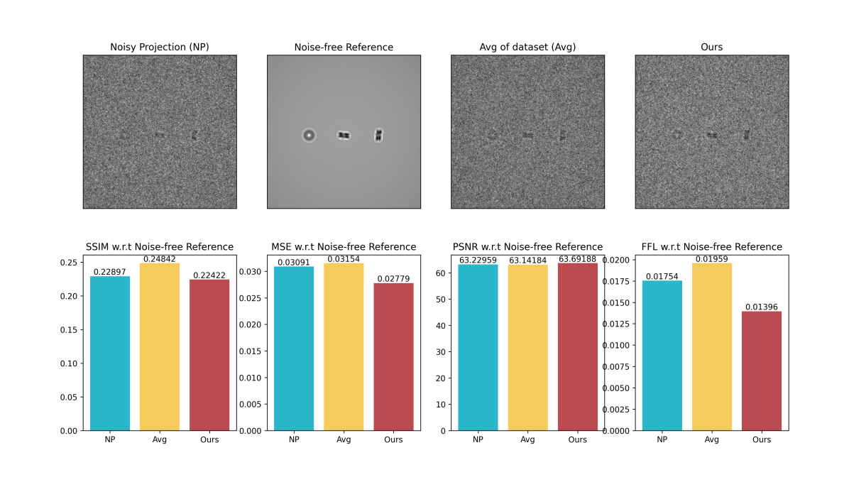
Figure 12: Denoising visual and quantitative comparison of synthetic data with data setting (200, 2)

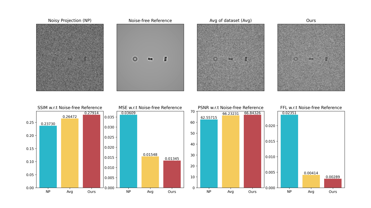
Figure 13: Denoising visual and quantitative comparison of synthetic data with data setting (200, 5)

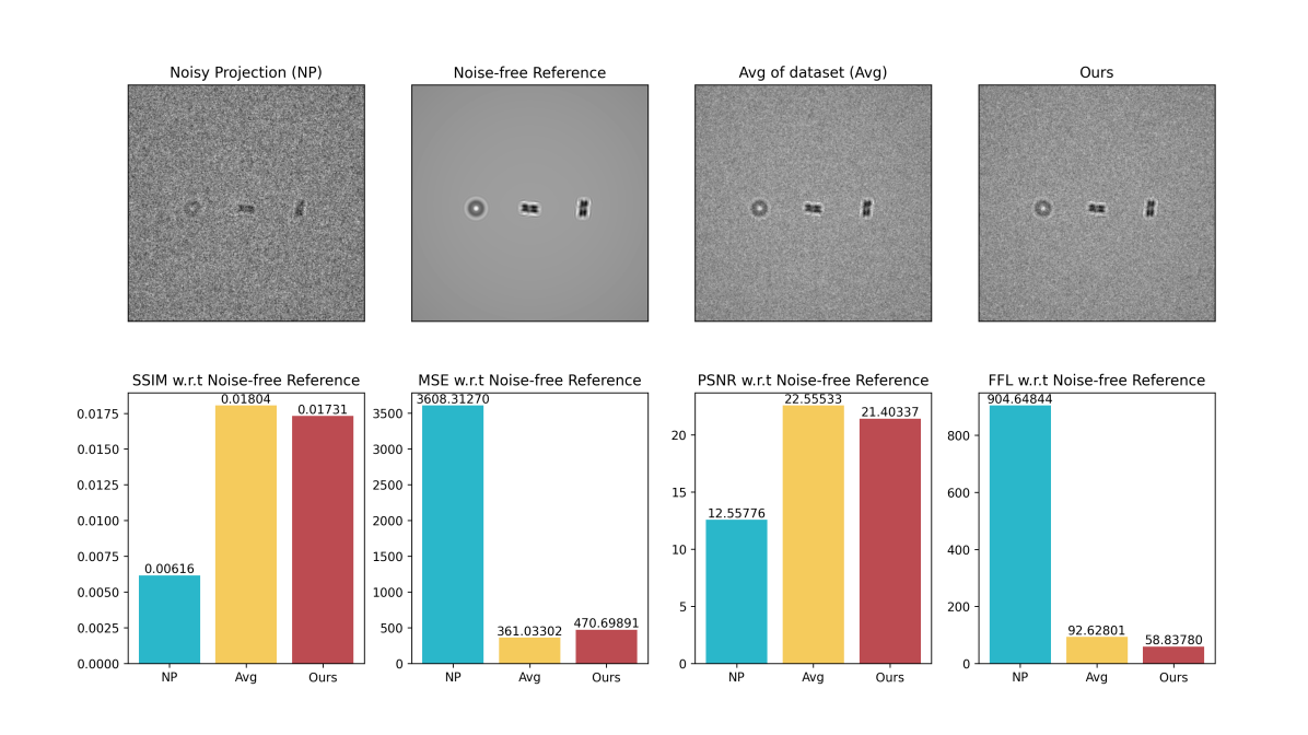
Figure 14: Denoising visual and quantitative comparison of synthetic data with data setting (700, 10)

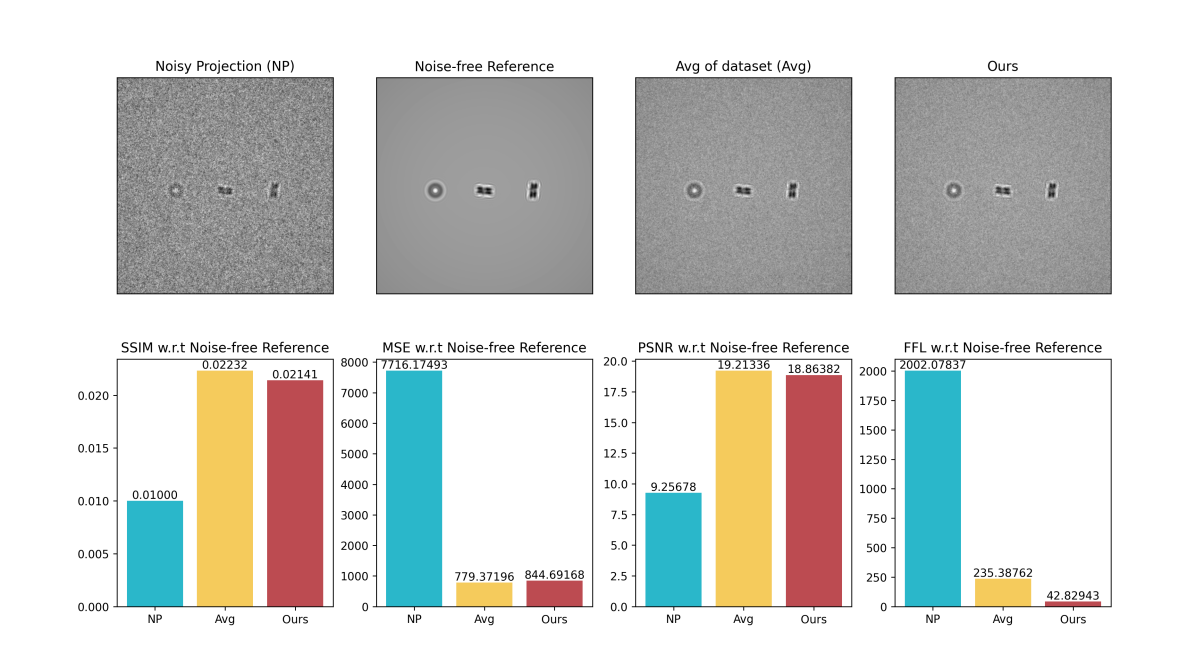
Figure 15: Denoising visual and quantitative comparison of synthetic data with data setting (1500, 10)

References

- [1] Werner Kühlbrandt. The resolution revolution. Science, 343(6178):1443–1444, 2014.
- [2] Eva Nogales and Sjors HW Scheres. Cryo-em: a unique tool for the visualization of macromolecular complexity. Molecular cell, 58(4):677–689, 2015.
- [3] Martin Turk and Wolfgang Baumeister. The promise and the challenges of cryo-electron tomography. FEBS Letters, 594(20):3243–3261, 2020.
- [4] Hans Rullgård, L-G Öfverstedt, Sergey Masich, Bertil Daneholt, and Ozan Öktem. Simulation of transmission electron microscope images of biological specimens. Journal of microscopy, 243(3):234–256, 2011.
- [5] Miloš Vulović, Raimond BG Ravelli, Lucas J van Vliet, Abraham J Koster, Ivan Lazić, Uwe Lücken, Hans Rullgård, Ozan Öktem, and Bernd Rieger. Image formation modeling in cryo-electron microscopy. Journal of structural biology, 183(1):19–32, 2013.
- [6] Benjamin Himes and Nikolaus Grigorieff. Cryo-tem simulations of amorphous radiation-sensitive samples using multislice wave propagation. IUCrJ, 8(6), 2021.
- [7] I Lobato and D Van Dyck. Multem: A new multislice program to perform accurate and fast electron diffraction and imaging simulations using graphics processing units with cuda. Ultramicroscopy, 156:9–17, 2015.
- [8] John M Cowley and A F_ Moodie. The scattering of electrons by atoms and crystals. i. a new theoretical approach. Acta Crystallographica, 10(10):609–619, 1957.
- [9] Earl J Kirkland. Advanced Computing in Electron Microscopy. Springer, 3rd. edition, 2020.
- [10] Sebastian Weiss and Rüdiger Westermann. Differentiable direct volume rendering. IEEE Transactions on Visualization and Computer Graphics, 28(1):562–572, 2022.
- [11] Harshit Gupta, Michael T. McCann, Laurène Donati, and Michael Unser. CryoGAN: A New Reconstruction Paradigm for Single-Particle Cryo-EM Via Deep Adversarial Learning. IEEE Transactions on Computational Imaging, 7:759–774, 2021.
- [12] Ian Goodfellow, Jean Pouget-Abadie, Mehdi Mirza, Bing Xu, David Warde-Farley, Sherjil Ozair, Aaron Courville, and Yoshua Bengio. Generative Adversarial Nets. In Z. Ghahramani, M. Welling, C. Cortes, N. Lawrence, and K. Q. Weinberger, editors, Advances in Neural Information Processing Systems, volume 27. Curran Associates, Inc., 2014.
- [13] Wim Van Aarle, Willem Jan Palenstijn, Jan De Beenhouwer, Thomas Altantzis, Sara Bals, K Joost Batenburg, and Jan Sijbers. The astra toolbox: A platform for advanced algorithm development in electron tomography. Ultramicroscopy, 157:35–47, 2015.
- [14] Tzu-Mao Li, Miika Aittala, Frédo Durand, and Jaakko Lehtinen. Differentiable Monte Carlo Ray Tracing through Edge Sampling. ACM Trans. Graph. (Proc. SIGGRAPH Asia), 37(6):222:1–222:11, 2018.
- [15] Jon Hasselgren, Jacob Munkberg, Marco Salvi, Anjul Patney, and Aaron Lefohn. Neural Temporal Adaptive Sampling and Denoising. Computer Graphics Forum, 2020.
- [16] Abdullah Hamdi, Silvio Giancola, and Bernard Ghanem. MVTN: Multi-View Transformation Network for 3D Shape Recognition. In Proceedings of the IEEE/CVF International Conference on Computer Vision (ICCV), pages 1–11, October 2021.
- [17] Hannah Kniesel, Timo Ropinski, Tim Bergner, Kavitha Shaga Devan, Clarissa Read, Paul Walther, Tobias Ritschel, and Pedro Hermosilla. Clean implicit 3d structure from noisy 2d stem images. In Proc. Computer Vision and Pattern Recognition (CVPR), IEEE, 2022.
- [18] Jaakko Lehtinen, Jacob Munkberg, Jon Hasselgren, Samuli Laine, Tero Karras, Miika Aittala, and Timo Aila. Noise2Noise: Learning Image Restoration without Clean Data. In Jennifer Dy and Andreas Krause, editors, Proceedings of the 35th International Conference on Machine Learning, volume 80 of Proceedings of Machine Learning Research, pages 2965–2974. PMLR, 10–15 Jul 2018.
- [19] Tristan Bepler, Kotaro Kelley, Alex J. Noble, and Bonnie Berger. Topaz-Denoise: general deep denoising models for cryoEM and cryoET. Nature Communications, 11(1):5208, Oct 2020.
- [20] Shakir Mohamed, Mihaela Rosca, Michael Figurnov, and Andriy Mnih. Monte Carlo Gradient Estimation in Machine Learning. J. Mach. Learn. Res., 21(132):1–62, 2020.
- [21] Diederik P Kingma and Max Welling. Auto-Encoding Variational Bayes, 2014.
- [22] John Schulman, Nicolas Heess, Theophane Weber, and Pieter Abbeel. Gradient Estimation Using Stochastic Computation Graphs. In Proceedings of the 28th International Conference on Neural Information Processing Systems - Volume 2, NIPS’15, pages 3528–3536, Cambridge, MA, USA, 2015. MIT Press.
- [23] Achilleas S. Frangakis and Reiner Hegerl. Noise Reduction in Electron Tomographic Reconstructions Using Nonlinear Anisotropic Diffusion. Journal of Structural Biology, 135(3):239–250, 2001.
- [24] XR Huang, S Li, and S Gao. [Progress in filters for denoising cryo-electron microscopy images]. Beijing da xue xue bao. Yi xue ban = Journal of Peking University. Health sciences, 53(2):425–433, March 2021.
- [25] Tim-Oliver Buchholz, Mareike Jordan, Gaia Pigino, and Florian Jug. Cryo-care: Content-aware image restoration for cryo-transmission electron microscopy data. In 2019 IEEE 16th International Symposium on Biomedical Imaging (ISBI 2019), pages 502–506, 2019.
- [26] Hongjia Li, Hui Zhang, Xiaohua Wan, Zhidong Yang, Chengmin Li, Jintao Li, Renmin Han, Ping Zhu, and Fa Zhang. Noise-Transfer2Clean: denoising cryo-EM images based on noise modeling and transfer. Bioinformatics, 02 2022.
- [27] Helen Berman, Kim Henrick, and Haruki Nakamura. Announcing the worldwide protein data bank. Nature structural biology, 10(12):980, 2003.
- [28] Duccio Fanelli and Ozan Öktem. Electron tomography: a short overview with an emphasis on the absorption potential model for the forward problem. Inverse Problems, 24(1):013001, 2008.
- [29] Walter Schottky. Über spontane stromschwankungen in verschiedenen elektrizitätsleitern. Annalen der physik, 362(23):541–567, 1918.
- [30] Barnaby DA Levin. Direct detectors and their applications in electron microscopy for materials science. Journal of Physics: Materials, 4(4):042005, 2021.
- [31] JM Zuo. Electron detection characteristics of a slow-scan ccd camera, imaging plates and film, and electron image restoration. Microscopy research and technique, 49(3):245–268, 2000.
- [32] NVIDIA, Péter Vingelmann, and Frank H.P. Fitzek. Cuda, release: 10.2.89, 2020.
- [33] Adam Paszke, Sam Gross, Francisco Massa, Adam Lerer, James Bradbury, Gregory Chanan, Trevor Killeen, Zeming Lin, Natalia Gimelshein, Luca Antiga, et al. Pytorch: An imperative style, high-performance deep learning library. Advances in neural information processing systems, 32, 2019.
- [34] Yuanming Hu, Tzu-Mao Li, Luke Anderson, Jonathan Ragan-Kelley, and Frédo Durand. Taichi: a language for high-performance computation on spatially sparse data structures. ACM Transactions on Graphics (TOG), 38(6):201, 2019.
- [35] Yuanming Hu, Luke Anderson, Tzu-Mao Li, Qi Sun, Nathan Carr, Jonathan Ragan-Kelley, and Frédo Durand. DiffTaichi: Differentiable Programming for Physical Simulation. ICLR, 2020.
- [36] Liming Jiang, Bo Dai, Wayne Wu, and Chen Change Loy. Focal frequency loss for image reconstruction and synthesis. In Proceedings of the IEEE/CVF International Conference on Computer Vision, pages 13919–13929, 2021.
- [37] Diederik P Kingma and Jimmy Ba. Adam: A method for stochastic optimization. arXiv preprint arXiv:1412.6980, 2014.
- [38] G. Bradski. The OpenCV Library. Dr. Dobb’s Journal of Software Tools, 2000.
- [39] Hangping Yao, Yutong Song, Yong Chen, Nanping Wu, Jialu Xu, Chujie Sun, Jiaxing Zhang, Tianhao Weng, Zheyuan Zhang, Zhigang Wu, Linfang Cheng, Danrong Shi, Xiangyun Lu, Jianlin Lei, Max Crispin, Yigong Shi, Lanjuan Li, and Sai Li. Molecular Architecture of the SARS-CoV-2 Virus. Cell, 183(3):730–738, 2020.
- [40] Ngan Nguyen, Ondřej Strnad, Tobias Klein, Deng Luo, Ruwayda Alharbi, Peter Wonka, Martina Maritan, Peter Mindek, Ludovic Autin, David S Goodsell, et al. Modeling in the time of covid-19: Statistical and rule-based mesoscale models. IEEE transactions on visualization and computer graphics, 27(2):722, 2021.
- [41] Zhou Wang, A.C. Bovik, H.R. Sheikh, and E.P. Simoncelli. Image quality assessment: from error visibility to structural similarity. IEEE Transactions on Image Processing, 13(4):600–612, 2004.
- [42] James R Kremer, David N Mastronarde, and J Richard McIntosh. Computer visualization of three-dimensional image data using imod. Journal of structural biology, 116(1):71–76, 1996.