Tangent ray foliations and their associated outer billiards

Abstract

Let $v$ be a unit vector field on a complete, umbilic (but not totally geodesic) hypersurface $N$ in a space form; for example on the unit sphere $S^{2k-1}\subset\mathbb{R}^{2k}$, or on a horosphere in hyperbolic space. We give necessary and sufficient conditions on $v$ for the rays with initial velocities $v$ (and $-v$) to foliate the exterior $U$ of $N$. We find and explore relationships among these vector fields, geodesic vector fields, and contact structures on $N$.

When the rays corresponding to each of $\pm v$ foliate $U$, $v$ induces an outer billiard map whose billiard table is $U$. We describe the unit vector fields on $N$ whose associated outer billiard map is volume preserving. Also we study a particular example in detail, namely, when $N\simeq\mathbb{R}^{3}$ is a horosphere of the four-dimensional hyperbolic space and $v$ is the unit vector field on $N$ obtained by normalizing the stereographic projection of a Hopf vector field on $S^{3}$. In the corresponding outer billiard map we find explicit periodic orbits, unbounded orbits, and bounded nonperiodic orbits. We conclude with several questions regarding the topology and geometry of bifoliating vector fields and the dynamics of their associated outer billiards.

Key words and phrases: bifoliation, geodesic fibration, Hopf fibration, contact structure, outer billiards, volume-preservation.

Mathematics Subject Classification 2020: 53C12, 37C83, 53D10.

1 Motivation

We begin with a simple observation: given one of the two unit tangent vector fields on the unit circle $S^{1}\subset\mathbb{R}^{2}$, the corresponding tangent rays foliate the exterior of $S^{1}\subset\mathbb{R}^{2}$. This leads to the following question.

Question 1.

What conditions on a unit tangent vector field on $S^{2k-1}\subset\mathbb{R}^{2k}$ guarantee that the corresponding tangent rays foliate the exterior of $S^{2k-1}$?

Prototypical examples arise from great circle fibrations of $S^{2k-1}$, for example, the standard Hopf fibrations. Indeed, each great circle $C$ can be written as the intersection of $S^{2k-1}$ with a $2$-plane $P_{C}$. Since no two great circles intersect, the exterior of $S^{2k-1}$ can be foliated using the corresponding collection of planes, and the exterior of $C$ in each such plane $P_{C}$ is foliated by the rays tangent to $C$. In this way, Question 1 is related to the study of geodesic fibrations of spheres.

Our interest in Question 1 also stems from the fact that skew geodesic fibrations of Euclidean space (that is, fibrations of $\mathbb{R}^{n}$ by nonparallel straight lines) can only exist for odd $n$. Therefore the tangent ray foliations we study here may be viewed as an even-dimensional counterpart to the odd-dimensional phenomenon of skew line fibrations.

Additional motivation for Question 1 arises from the study of outer billiards. As suggested by its name, outer billiards is played outside a smooth closed strictly convex curve $\gamma\subset\mathbb{R}^{2}$, and can be easily defined as follows: fix one of the two unit tangent vector fields $v$ on $\gamma$, and observe that the corresponding tangent rays foliate the exterior of $\gamma$. In particular, for each point $x$ outside of $\gamma$, there exists exactly one tangent ray passing through $x$, and the outer billiard map $B$ is defined by reflecting $x$ about the point of tangency (see Figure 1). Originally popularized by Moser [20, 21], who studied the outer billiard map as a crude model for planetary motion, the outer billiard has since been studied in a number of contexts; see [3, 25, 26, 28] for surveys.

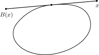
Figure 1: The outer billiard map in the plane

When attempting to define outer billiards in higher dimensional Euclidean space, one encounters the following issue: given a smooth closed strictly convex hypersurface $N$, there are too many tangent lines passing through each point $x$ outside of $N$, and so it is not obvious how to define outer billiards with respect to $N$. In [27], Tabachnikov resolved this issue in even-dimensional Euclidean space $\mathbb{R}^{2k}$, endowed with the standard symplectic structure $\omega$, by appealing to the characteristic line bundle $\xi\coloneqq\operatorname{ker}(\omega|_{N})$ on $N$. This line bundle $\xi$ has two unit sections $\pm v$, and each has the property that the corresponding tangent rays foliate the exterior of $N$. Thus choosing either $v$ or $-v$ yields a well-defined, invertible outer billiard map on the exterior of $N$; moreover, Tabachnikov proved that this outer billiard map is a symplectomorphism with respect to $\omega$. As an example, when $N=S^{2k-1}$, the characteristic lines are tangent to the great circles of the Hopf fibration.

We emphasize that the essential ingredient in the outer billiard construction is that the tangent rays corresponding to both $\pm v$ foliate the exterior of $N$. Thus an additional motivation for Question 1 is the construction of outer billiard systems which may exhibit interesting dynamical properties.

2 Statement of results

Our main result not only provides a complete answer to Question 1, but it also applies to the more general situation in which the ambient Euclidean space is replaced by the $(n+1)$-dimensional space form $M_{\kappa}$ of constant sectional curvature $\kappa$, and the role of the sphere $S^{n}\subset\mathbb{R}^{n+1}$ is played by a complete umbilic hypersurface $N\subset M_{\kappa}$ which is not totally geodesic (recall that $N\subset M_{\kappa}$ is umbilic if all of its principal curvatures are equal). In particular, the sectional curvature of $N$ is constant and strictly larger than $\kappa$ (as a corollary of the Gauss Theorem, see for instance Remark 2.6 in Chapter 6 of [2]).

Specifically, we will consider Question 1 in the following five settings:

1. $\kappa=0$: $M_{0}=\mathbb{R}^{n+1}$, and $N$ is an $n$-dimensional round sphere,

2. $\kappa>0$: $M_{\kappa}$ is a round sphere and $N$ is a geodesic sphere which is not a great sphere; that is, its curvature is larger than $\kappa$,

3. $\kappa<0$: $M_{\kappa}$ is the $(n+1)$-dimensional hyperbolic space $H^{n+1}$. It is convenient to describe the umbilics in the upper-half space model $\left\{(x_{0},\dots,x_{n})\in\mathbb{R}^{n+1}\mid x_{0}>0\right\}$ with the metric $ds^{2}=(dx_{0}^{2}+\cdots+dx_{n}^{2})/(-\kappa x_{0}^{2})$. The umbilic hypersurfaces are then the intersections with $H^{n+1}$ of hyperspheres and hyperplanes in $\mathbb{R}^{n+1}$, and there are three possibilities for $N$:

   1. $N$ is a geodesic sphere,

   2. $N$ is a horosphere, which is congruent by an isometry to $x_{0}=1$,

   3. $N$ is congruent by an isometry to the intersection of $H^{n+1}$ with a hyperplane through the origin which is not orthogonal to the hyperplane $x_{0}=0$.

Observe that in each case, $N$ is diffeomorphic to a sphere or to Euclidean space.

Next, we define the exterior $U$ of $N$ as the connected component of $M_{\kappa}-N$ into which the opposite of the mean curvature vector field of $N$ points, except that for $\kappa>0$, we further restrict $U$ to be the zone between $N$ and its antipodal image. The exterior $U$ in each of the five situations is depicted in Figure 2.

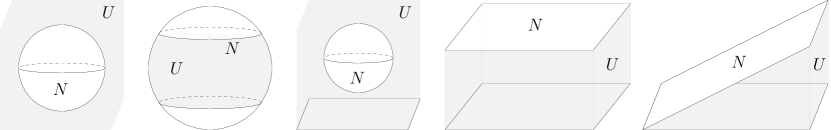
Figure 2: The exterior $U$, from left to right, for $\kappa=0$, $\kappa>0$, and $\kappa<0$

Given $u\in TM_{\kappa}$, we denote by $\gamma_{u}$ the unique geodesic in $M_{\kappa}$ with initial velocity $u$, and we write $T_{\kappa}=\infty$ for $\kappa\leq 0$ and $T_{\kappa}=\pi/\sqrt{\kappa}$ for $\kappa>0$. Note that a unit speed geodesic of the sphere tangent to $N$ at $p$ travels through $U$ and hits $-p\in-N$ at time $T_{\kappa}$.

Definition 2.

Let $v$ be a smooth unit vector field on a complete umbilic hypersurface $N$ of $M_{\kappa}$ which is not totally geodesic, and let $U$ be the exterior of $N$ as defined above. We say that $v$:

• forward foliates $U$ if the geodesic rays $\gamma_{v\left(p\right)}\left(0,T_{\kappa}\right)$ are the leaves of a smooth foliation of $U$,

• backward foliates $U$ if the geodesic rays $\gamma_{-v\left(p\right)}\left(0,T_{\kappa}\right)$ are the leaves of a smooth foliation of $U$,

• bifoliates $U$ if $v$ both forward and backward foliates $U$.

While a forward or backward foliation induces a dynamical system which may not be time-reversible, a bifoliation induces a smooth, invertible outer billiard map on $U$ (see (1) for the definition), justifying our interest in this specific notion.

With all of the terminology introduced above, Question 1 admits the following general formulation:

Question $\mathbf{1^{\prime}}$.

Let $U$ be the exterior of a complete umbilic not totally geodesic hypersurface $N$ in $M_{\kappa}$. What conditions on a smooth unit vector field $v$ on $N$ guarantee that $v$ bifoliates $U$?

We denote by $\nabla$ the Levi-Civita connection on $N$. Observe that since $v$ has unit length, the image of $\left(\nabla v\right)_{p}$ is orthogonal to $v(p)$ for every $p\in N$. In particular, $\left(\nabla v\right)_{p}$ is singular and preserves the subspace $v(p)^{\perp}\subset T_{p}N$.

We now provide a complete classification of bifoliating vector fields.

Theorem 3.

Let $U$ be the exterior of a complete umbilic not totally geodesic hypersurface $N$ in $M_{\kappa}$ and let $v$ be a smooth unit vector field on $N$. Then the assertions below are equivalent:

1. The vector field $v$ bifoliates $U$.

2. For each $p\in N$, any real eigenvalue $\lambda$ of the restriction of the operator $\left(\nabla v\right)_{p}$ to $v(p)^{\perp}\subset T_{p}N$ satisfies $\lambda^{2}+\kappa\leq 0$.

3. For each $p\in N$ and any real eigenvalue $\lambda$ of $\left(\nabla v\right)_{p}$, the following condition holds:

   1. for $\kappa=0$: $\lambda=0$;

   2. for $\kappa>0$: $\lambda=0$ with algebraic multiplicity one;

   3. for $\kappa<0$: $\lambda^{2}\leq-\kappa$.

Remark.

Although Theorem 3 is written without explicit topological restrictions on $N$, the existence of $v$ implies that $N$ is not an even-dimensional sphere.

Remark.

We emphasize a surprising feature of Theorem 3: the global condition that $v$ bifoliates $U$ is characterized by an infinitesimal condition on $v$, which one might expect to only guarantee a smooth foliation locally.

Remark.

Looking at the proof of Theorem 3 one can easily deduce conditions for a unit vector field on $N$ to forward or backward foliate the exterior.

At the beginning of Section 1 we observed that great circle fibrations of odd-dimensional spheres induce bifoliating vector fields. This statement persists in the general setting. A geodesic vector field on $N$ is a unit vector field on $N$ whose integral curves are geodesics. Using the explicit criterion of Theorem 3, we show that geodesic vector fields are bifoliating, but not all bifoliating vector fields are geodesic.

Theorem 4.

Let $U$ be the exterior of a complete umbilic not totally geodesic hypersurface $N$ in $M_{\kappa}$.

1. If a smooth unit vector field $v$ on $N$ is geodesic, then $v$ is bifoliating.

2. If $n>1$, there exists a smooth bifoliating vector field on $N$ which is not geodesic.

The latter statement is credible for the following simple reason: for $\kappa\geq 0$, the vector field $v$ tangent to the Hopf fibration on $N=S^{2k+1}$ is both bifoliating and geodesic, but an arbitrarily small perturbation can ruin the symmetry of the integral curves while maintaining the open condition that the restriction of the operator $\left(\nabla v\right)_{p}$ to $v(p)^{\perp}\subset T_{p}N$ has no real eigenvalues. This idea motivates the explicit examples which we provide in the proof of Theorem 4.

A geodesic vector field on a Riemannian manifold $M$ determines an oriented geodesic foliation of $M$. In this language, Theorem 4 says that a geodesic vector field on $N$ determines both a geodesic foliation of $N$ itself and a bifoliation of the exterior $U$, but that some bifoliations of $U$ arise from vector fields on $N$ which do not determine geodesic foliations.

Geodesic foliations of the space forms $M_{\kappa}$ are of interest in their own right and have been studied extensively. Great circle fibrations of $S^{3}$ are characterized in [7] and studied in higher dimensions in [8, 19]. Geodesic foliations of $\mathbb{R}^{3}$ and hyperbolic space $H^{3}$ have been characterized in [12, 16, 17, 22, 24]. In [5], Gluck proved that the plane field orthogonal to a great circle fibration of $S^{3}$ is a tight contact structure. The relationship between line fibrations of $\mathbb{R}^{3}$ and (tight) contact structures was studied in [1, 15, 16]. We show that a similar relationship exists for bifoliating vector fields.

Theorem 5.

Let $v$ be a smooth bifoliating unit vector field on a sphere $N\subset S^{4}$. Then the $1$-form dual to $v$ is a contact form.

Remarks.

We make several remarks to contextualize Theorem 5.

1. By Theorem 3, every bifoliating vector field $v$ on $N\subset S^{4}$ satisfies a certain condition, namely, that $\left(\nabla v\right)_{p}$ has rank $2$ for all $p\in S^{3}$. Bifoliating vector fields on $S^{3}\subset\mathbb{R}^{4}$ do not necessarily satisfy this nondegeneracy condition; see Proposition 14 for an example. However, Theorem 5 and its proof do hold for smooth bifoliating vector fields on $S^{3}\subset\mathbb{R}^{4}$ if the condition is added as a hypothesis.

2. Theorem 5 fails in higher dimensions for $\kappa\geq 0$. In [9], Gluck and Yang construct examples of unit vector fields on $S^{n}$, for odd $n\geq 5$, which determine great circle fibrations (and thus are bifoliating by Theorem 4) for which the dual form is not contact.

3. Theorem 5 fails for the horosphere in hyperbolic space, since a constant vector field is bifoliating, but the dual $1$-form is not contact.

4. We do not know if the contact structures in Theorem 5 are tight; see Question 18 for discussion.

We now turn our attention to the dynamical properties exhibited by bifoliating vector fields. A bifoliating vector field $v$ on $N$ induces an outer billiard map $B\colon U\rightarrow U$ defined by

$$B(\gamma_{v(p)}(-t))=\gamma_{v(p)}(t),\hskip 18.06749pt(p,t)\in N\times(0,T_{\kappa}).$$ (1)

See Figure 3 for a depiction in hyperbolic space.

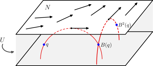
Figure 3: Two iterations of the outer billiard map induced by a bifoliating vector field on a horosphere $N$, seen in the upper-half space model of hyperbolic space

Typically, the dynamics of billiard systems can be studied via their symplectic properties. However, the outer billiard systems induced by bifoliating vector fields are, in general, not symplectic. It seems plausible that different techniques are necessary for a careful study of their dynamics.

On the other hand, we study a particular example in detail, for which $N\simeq\mathbb{R}^{3}$ is a horosphere in $H^{4}$ and $v$ is the unit vector field obtained by normalizing the stereographic projection of the Hopf vector field on $S^{3}$. For the associated outer billiard map we find explicit periodic orbits, unbounded orbits, and bounded nonperiodic orbits; see Proposition 17.

We conclude by studying the relationship between volume-preservation of $B$ and the characteristic polynomials $Q_{p}(s)\coloneqq\det\left(s~{}\text{id}_{T_{p}N}-\left(\nabla v\right)_{p}\right)$ of $\left(\nabla v\right)_{p}$ for $p\in N$.

Theorem 6.

Let $U$ be the exterior of a complete umbilic not totally geodesic $n$-dimensional hypersurface $N$ in $M_{\kappa}$ and let $v$ be a smooth bifoliating unit vector field on $N$. Then the associated outer billiard map $B\colon U\to U$ be preserves volume if and only if, for all $p\in N$ and $s\in\mathbb{R}$,

$$Q_{p}(-s)=\left(-1\right)^{n}Q_{p}(s);$$

that is, for all $p$, the parity of $Q_{p}$ coincides with the parity of $n$.

Corollary 7.

Let $U$ be the exterior of a complete umbilic not totally geodesic $n$-dimensional hypersurface $N$ in $M_{\kappa}$, and let $B\colon U\to U$ be the outer billiard map associated to a bifoliating unit vector field $v$ on $N$.

1. If the map $B$ preserves volume, then $\operatorname{div}v$ vanishes identically, that is, the flow of $v$ preserves the volume of $N$. If additionally $n$ is even, then the restriction of $\left(\nabla v\right)_{p}$ to $v(p)^{\perp}$ is singular for all $p\in N$.

2. If $n=2$ (which implies that $\kappa<0$, $N$ is diffeomorphic to $\mathbb{R}^{2}$, and its intrinsic metric has constant Gaussian curvature $k$ with $\kappa<k\leq 0$), then the following are equivalent:

   1. the map $B$ preserves volume,

   2. $v$ is orthogonal to a geodesic foliation of $N$,

   3. $\operatorname{div}v$ vanishes identically.

   If $N\simeq\mathbb{R}^{2}\subset H^{3}$ is a horosphere, the above conditions are equivalent to $v$ being constant.

3. If $n=3$, then the map $B$ preserves volume if and only if $\operatorname{div}v$ vanishes identically. If additionally $N=S^{3}$ and $v$ is geodesic (that is, $v$ determines a great circle fibration), then $B$ preserves volume if and only if $v$ is Hopf.

We comment that the normalization of a nowhere vanishing Killing field on $N\subset H^{3}$ provides an example of a vector field satisfying the conditions in (b).

3 Preliminaries on Jacobi fields

Here we provide a brief review of Jacobi fields, which arise naturally when studying variations of geodesics, and thus play a central role in the proofs of the main theorems. A more thorough treatment can be found in any standard Riemannian geometry text, for example [2].

Let $M$ be a complete Riemannian manifold and let $\gamma$ be a complete unit speed geodesic of $M$. A Jacobi field $J$ along $\gamma$ is by definition a vector field along $\gamma$ arising via a variation of geodesics as follows: Let $\delta>0$ and $\phi\colon\mathbb{R}\times(-\delta,\delta)\rightarrow M$ be a smooth map such that $s\mapsto\phi(s,t)$ is a geodesic for each $t\in(-\delta,\delta)$ and $\phi(s,0)=\gamma(s)$ for all $s$. Then

$$J(s)=\left.\frac{d}{dt}\right|_{0}\phi(s,t).$$

When $M=M_{\kappa}$, it is well known that Jacobi fields along a unit speed geodesic $\gamma$ and orthogonal to $\gamma^{\prime}$ are exactly those vector fields $J$ along $\gamma$ with $\left\langle J,\gamma^{\prime}\right\rangle=0$ satisfying the equation

$$\frac{D^{2}J}{ds^{2}}+\kappa J=0.$$ (2)

If the initial conditions of $J$ are $J(0)=a\gamma^{\prime}(0)+u$ and $\frac{DJ}{dt}(0)=w$, with $a\in\mathbb{R}$ and $u,w$ orthogonal to $\gamma^{\prime}(0)$, then

$$J(t)=a\gamma^{\prime}(t)+c_{\kappa}(t)U(t)+s_{\kappa}(t)W(t),$$ (3)

where $U,W$ are parallel vector fields along $\gamma$ with $U\left(0\right)=u$ and $W\left(0\right)=w$,

$$s_{\kappa}\left(t\right)=\left\{\begin{array}[]{ll}\sin\left(\sqrt{\kappa}t\right)/\sqrt{\kappa}&\text{if }\kappa>0,\\ t&\text{if }\kappa=0,\\ \sinh\left(\sqrt{-\kappa}t\right)/\sqrt{-\kappa}&\text{if }\kappa<0,\end{array}\right.\text{\ \ \ \ \ \ \ \ \ and }\hskip 7.11317ptc_{k}(t)=s_{k}^{\prime}(t).$$ (4)

Also, we call $\cot_{\kappa}=c_{\kappa}/s_{\kappa}$. Expression (3) will allow us to perform most computations without having to resort to coordinates of $M_{\kappa}$ or a particular model of it.

Lemma 8.

Let $\lambda\in\mathbb{R}$. If $\lambda^{2}+\kappa>0$, then the equation $c_{\kappa}(t)-\left|\lambda\right|s_{\kappa}(t)=0$ has a solution in the interval $\left(0,T_{\kappa}\right)$.

Proof.

The assertion follows from the fact that for $\kappa=0$, $\kappa>0$ and $\kappa<0$, the equation reads $\left|\lambda\right|t=1$, $\cot\left(\sqrt{\kappa}t\right)=\left|\lambda\right|/\sqrt{\kappa}$ and $\coth\left(\sqrt{-\kappa}t\right)=\left|\lambda\right|/\sqrt{-\kappa}$, respectively. ∎

Lemma 9.

Let $M$ be a Riemannian manifold and let $\phi:\left(-\varepsilon,\varepsilon\right)\times\left(0,T\right)\rightarrow M$ be a geodesic variation, that is, $\gamma_{s}:\left(0,T\right)\rightarrow M$ is a unit speed geodesic in $M$ for all $s\in\left(-\varepsilon,\varepsilon\right)$, where $\gamma_{s}\left(t\right)=\phi\left(s,t\right)$. Suppose that $V$ is a unit vector field on $M$ such that $V\left(\gamma_{s}\left(t\right)\right)=\gamma_{s}^{\prime}\left(t\right)$ for all $s,t$. Then the Jacobi field along $\gamma_{0}$ associated with $\phi$ vanishes at some $t_{o}\in\left(0,T\right)$ only if it is identically zero.

Proof.

We call $\beta\left(s\right)=\phi\left(s,t_{o}\right).$ We have that $0=J\left(t_{o}\right)=\beta^{\prime}\left(0\right)$. We compute

$$\frac{DJ}{dt}(t_{o}) = \left.\frac{D}{\partial t}\right|_{t_{o}}\left.\frac{\partial}{\partial s}\right|_{0}\phi\left(s,t\right)=\left.\frac{D}{\partial s}\right|_{0}\left.\frac{\partial}{\partial t}\right|_{t_{o}}\gamma_{s}\left(t\right)$$

$$= \left.\frac{D}{\partial s}\right|_{0}\gamma_{s}^{\prime}\left(t_{o}\right)=\left.\frac{D}{\partial s}\right|_{0}V(\beta(s))=\nabla_{\beta^{\prime}(0)}V=0.$$

Since $J$ is the solution of a second order differential equation, $J\equiv 0$, as desired. ∎

4 Bifoliations and the proof of Theorem 3

We now return to the situation in which $N$ is a complete umbilic hypersurface of $M_{\kappa}$ which is not totally geodesic. Recall that a complete list of such pairs $(M_{\kappa},N)$ was given at the beginning of Section 2. We denote by $\overline{\nabla}$ and $\nabla$ the Levi-Civita connections of $M_{\kappa}$ and $N$, respectively. The Gauss formula in this case is given by

$$\overline{\nabla}_{X}Y=\nabla_{X}Y+\langle X,Y\rangle_{\kappa}H,\hskip 18.06749ptX,Y\in\mathfrak{X}(N),$$ (5)

where $H$ is the mean curvature vector field on $N$. Unless otherwise stated, geodesics are always in $M_{\kappa}$.

Now let $v$ be a unit vector field on $N$. For $t\in\left(0,T_{\kappa}\right)$, we define

$$f_{t}\colon N\to M_{\kappa},\hskip 36.135ptf_{t}(p)=\gamma_{v\left(p\right)}(t).$$

We first concentrate on the image of $f_{t}$.

Let $G_{\kappa}=$ Iso${}_{o}(M_{\kappa})$ be the identity component of the isometry group of $M_{\kappa}$ and let $L=\left\{g\in G_{\kappa}\mid g(N)=N\right\}$, which is isomorphic to Iso${}_{o}(N)$. When $N$ is a sphere, there are one or two trivial orbits of $L$ (depending on the ambient space); otherwise, the orbits of $L$ are the parallel hypersurfaces to $N$, which are well-known to be umbilic.

Lemma 10.

For each $t\in(0,T_{\kappa})$, the image of $f_{t}$ is contained in exactly one hypersurface parallel to $N$.

Proof.

Let $p,q\in N$. Since $N$ is extrinsically two-point homogeneous, there exists $h\in L$ such that $h(p)=q$ and $dh_{p}\,v(p)=v(q)$. So,

$$f_{t}(q)=\gamma_{v\left(q\right)}(t)=\gamma_{dh_{p}v(p)}(t)=h(\gamma_{v\left(p\right)}(t))=h(f_{t}(p)),$$

as desired. ∎

Now for $t\in(0,T_{\kappa})$, we define $N_{t}$ as the hypersurface parallel to $N$ which contains the image of $f_{t}$. Since $N_{t}$ is embedded, the map $f_{t}\colon N\to N_{t}$ is smooth. We next compute its differential.

Lemma 11.

Let $v$ be a unit vector field on $N$. Let $p\in N$ and $x=av\left(p\right)+u\in T_{p}N$, with $a\in\mathbb{R}$ and $u\perp v\left(p\right)$. Then

$$\left(df_{t}\right)_{p}\left(x\right)=\tau_{0}^{t}\left(av(p)+\left(c_{\kappa}(t)u+s_{\kappa}(t)\nabla_{x}v\right)+s_{\kappa}(t)aH\left(p\right)\right),$$ (6)

where $\tau_{0}^{t}$ denotes the parallel transport along $\gamma_{v(p)}$ between $0$ and $t$.

Proof.

Let $\alpha$ be a smooth curve in $N$ with $\alpha^{\prime}(0)=x$. Let $J$ be the Jacobi field along $\gamma_{v(p)}$ associated with the geodesic variation $\left(s,t\right)\mapsto\gamma_{v(\alpha(s))}(t)$. We have $J(0)=x$ and, with an argument similar to that in the proof of Lemma 9,

$$\frac{DJ}{dt}(0)=\overline{\nabla}_{x}v.$$

So $J$ depends only on $x$ and we call it $J_{x}$. By (3) and (5),

$$J_{x}(t)=a\gamma_{v(p)}^{\prime}(t)+c_{\kappa}(t)\tau_{0}^{t}(u)+s_{\kappa}(t)\tau_{0}^{t}(\nabla_{x}v+aH(p)).$$ (7)

Then

$$(df_{t})_{p}\left(x\right)=\left.\frac{d}{ds}\right|_{0}f_{t}\left(\alpha\left(s\right)\right)=J_{x}(t)$$

and the lemma follows. ∎

Proposition 12.

If for each $p\in N$ any real eigenvalue $\lambda$ of the restriction of the operator $\left(\nabla v\right)_{p}$ to $v\left(p\right)^{\perp}\subset T_{p}N$ satisfies $\lambda^{2}+\kappa\leq 0$, then $f_{t}:N\rightarrow N_{t}$ is a diffeomorphism.

Proof.

We prove first that $f_{t}$ is a local diffeomorphism. To argue the contrapositive, suppose that $(df_{t})_{p}(x)=0$ for some $x\neq 0$. Since the three terms on the right hand side of (6) are pairwise orthogonal, we conclude that $a=0$ (in particular, $x=u$) and $c_{\kappa}(t)x+s_{\kappa}(t)\nabla_{x}v=0$. Hence,

$$\nabla_{x}v=-\cot_{\kappa}(t)x\text{,}$$

that is, $x\in v(p)^{\perp}$ is an eigenvector of $(\nabla v)_{p}$ with eigenvalue $-\cot_{\kappa}t$. Together with the observation that $\cot_{\kappa}^{2}(t)+\kappa>0$ holds for all $\kappa$, this completes the argument.

Next we prove that $f_{t}:N\rightarrow N_{t}$ is a diffeomorphism. For $N=S^{1}$, the assertion is clear. If $N$ is a sphere different from the circle, then, by compactness, $f_{t}$ is a covering map, which must be a bijection since $N$ is simply connected.

If $N$ is not a sphere, then $\kappa<0$ and both $N$ and $N_{t}$ are diffeomorphic to $\mathbb{R}^{n}$. To see that $f_{t}$ is a diffeomorphism, we apply a “global inverse” result of Hadamard (see [18, Theorem 6.2.8] or [13]), which asserts that a smooth proper local diffeomorphism from $\mathbb{R}^{n}$ to $\mathbb{R}^{n}$ is a diffeomorphism; here proper means that the preimage of every compact set is compact. Properness of $f_{t}$ follows from the facts that $f_{t}$ displaces each point by distance $t$ (in $M_{\kappa}$) and that $N$ is properly embedded in $M_{\kappa}$. Hence $f_{t}$ is a diffeomorphism. ∎

We are now prepared to prove Theorem 3.

Proof of Theorem 3.

“(a) $\Rightarrow$ (b)” Let $\lambda\in\mathbb{R}$ and suppose there exists a nonzero tangent vector $u\in v\left(p\right)^{\perp}\subset T_{p}N$ such that $\nabla_{u}v=\lambda u$. We consider the Jacobi vector field

$$J(t)=\left.\frac{d}{ds}\right|_{0}\gamma_{v(\alpha(s))}(t)\text{,}$$

where $\alpha$ is a smooth curve in $N$ with $\alpha^{\prime}\left(0\right)=u$. By (5) we have that $\nabla_{u}v=\overline{\nabla}_{u}v$ and so, $J(0)=u$ and $\frac{DJ}{dt}(0)=\lambda u$. Using (3), we obtain

$$J(t)=(c_{\kappa}(t)+\lambda s_{\kappa}(t))U(t)\text{,}$$

where $U$ is the parallel vector field along $\gamma_{v(p)}$ such that $U(0)=u$.

Now $J$ is associated with the variation given by the geodesic rays of the forward foliation of $U$, and Lemma 9 implies that $J$ does not vanish for any $t\in(0,T_{\kappa})$. Now if $\lambda\leq 0$, Lemma 8 applies and yields $\lambda^{2}+\kappa\leq 0$, as desired. In case $\lambda>0$, we instead consider the Jacobi field associated with the variation given by the geodesic rays $\gamma_{-v(\alpha(s))}(t)$ of the backward foliation of $U$ and proceed similarly.

“(b) $\Rightarrow$ (a)” To verify that the vector field $v$ bifoliates $U$, we show that $F_{+}$ and $F_{-}$ are diffeomorphisms, where $F_{+}$ and $F_{-}$ are the restrictions to $N\times(0,T_{\kappa})$ and $N\times(-T_{\kappa},0)$, respectively, of the smooth function

$$F\colon N\times(-T_{\kappa},T_{\kappa})\rightarrow M_{\kappa},\ \ \ \ F(p,s)=\gamma_{v\left(p\right)}(s).$$

We deal only with $F_{+}$, since the case of $F_{-}$ is analogous.

The map $F_{+}$ is a bijection by Proposition 12, since $f_{t}(N)=N_{t}$ for all $t\in\left(0,T_{\kappa}\right)$, and the umbilic hypersurfaces $N_{t}$ foliate $U$.

Now we check that $(dF_{+})_{(p,t)}$ is an isomorphism. By Proposition 12, it sends $T_{p}N\times\left\{0\right\}$ isomorphically to $T_{f_{t}\left(p\right)}N_{t}=\left(df_{t}\right)_{p}\left(T_{p}N\right)$. Hence, it suffices to show that

$$(dF_{+})_{(p,t)}\left(0,\left.\tfrac{\partial}{\partial s}\right|_{t}\right)=\gamma_{v\left(p\right)}^{\prime}\left(t\right)\not\in T_{f_{t}\left(p\right)}N_{t}\text{.}$$

Assume otherwise, so that $\gamma_{v\left(p\right)}^{\prime}\left(t\right)=\left(df_{t}\right)_{p}\left(x\right)$ for some $x\in T_{p}N$. Applying $\left(\tau_{0}^{t}\right)^{-1}$ to (6), we have

$$v\left(p\right)=av\left(p\right)+\left(c_{\kappa}(t)u+s_{\kappa}(t)\nabla_{x}v\right)+s_{\kappa}(t)aH(p)\text{.}$$

Now, the scalar product with $v(p)$ yields $a=1$, but the scalar product with $H(p)$ yields $a=0$ (indeed, $s_{\kappa}(t)H(p)\neq 0$, since $N$ is not totally geodesic and $s_{\kappa}$ does not vanish on $(0,T_{\kappa})$). This is a contradiction. Consequently, $(dF_{+})_{(p,t)}$ is an isomorphism.

Finally, the smooth vector field that gives the foliation $\{\gamma_{v(p)}(0,T_{\kappa})\,|\,p\in N\}$ of $U$ is given by $V=dF\circ\left(0,\tfrac{\partial}{\partial s}\right)\circ F^{-1}$.

“(b) $\Leftrightarrow$ (c)”: The equivalence of (b) and (c) follows from the following linear algebra lemma, with $T=\left(\nabla v\right)_{p}$ and $W=v\left(p\right)^{\perp}$. ∎

Lemma 13.

Let $T:V\rightarrow V$ be a linear transformation whose image is contained in the codimension one subspace $W$ (in particular, 0 is an eigenvalue of $T$) and let $S=\left.T\right|_{W}\colon W\rightarrow W$. Then $S$ has no real eigenvalues if and only if the only real eigenvalue of $T$ is zero with algebraic multiplicity one.

Proof.

The lemma is a consequence of the following two assertions:

1. A real number $\lambda\neq 0$ is an eigenvalue of $S$ if and only if $\lambda$ is an eigenvalue of $T$.

2. The map $S$ has eigenvalue $0$ if and only if $T$ has eigenvalue $0$ with algebraic multiplicity greater than one.

Both arguments are straightforward; we only write the details of (b).

Suppose that $0$ is an eigenvalue of $S$ with eigenvector $x\in W$. We may assume that the image of $T$ is equal to $W$, since otherwise $\dim\operatorname{ker}(T)\geq 2$, and the proof is complete. Thus $x=Ty$ for some $y\in V$, hence $y$ is a generalized eigenvector of $T$ (which must be linearly independent from $x$) and so the eigenvalue $0$ of $T$ has algebraic multiplicity at least $2$.

Conversely, suppose that $0$ is an eigenvalue of $T$ with algebraic multiplicity at least $2$. Then the subspace $\left\{y\in V\mid T^{2}y=0\right\}$ intersects $W$ nontrivially. If a nonzero vector $y\in W$ satisfies $T^{2}y=0$, then either $y$ or $Ty$ is a nonzero vector in $\operatorname{ker}(T)$, and hence in $\operatorname{ker}(S)$. ∎

5 Bifoliations and geodesic vector fields

Here we prove Theorem 4, that geodesic vector fields are bifoliating, but not all bifoliating vector fields are geodesic.

Proof of Theorem 4.

Let $v$ be a smooth unit vector field on $N\subset M_{\kappa}$. To show part (a), we assume that $v$ is geodesic and we verify that $v$ satisfies the criterion of Theorem 3(b).

Suppose that $N$ has constant sectional curvature $k$, in particular $k>\kappa$. Let $p\in N$, let $x$ be a unit vector in $T_{p}N$ orthogonal to $v(p)$, and suppose that $\nabla_{x}v=\lambda x$, with $\lambda\in\mathbb{R}$. As in the proof of (a) $\Rightarrow$ (b) of Theorem 3, but considering Jacobi fields on $N$ defined on $\left(0,T_{k}\right)$ along geodesics in $N$ (instead of $M_{\kappa}$), we obtain that $\lambda^{2}+k\leq 0$. Consequently, $\lambda^{2}+\kappa\leq 0$ and so $v$ is bifoliating by Theorem 3. This completes the proof of part (a).

We now prove part (b). We begin by constructing a unit vector field on the unit sphere $S^{2k-1}$ which is bifoliating in any ambient space but is not geodesic, obtained by perturbing the standard Hopf fibration.

Let $J\colon\mathbb{R}^{2k}\to\mathbb{R}^{2k}$ denote the standard almost complex structure, which we write explicitly as $J(p_{1},\dots,p_{2k})=(-p_{2},p_{1},\dots,-p_{2k},p_{2k-1})$. We define $P\colon\mathbb{R}^{2k}\to\mathbb{R}^{2k}$ by $P(p_{1},\dots,p_{2k})=(-p_{4},p_{3},-p_{2},p_{1},0,\dots,0)$ and the unit vector field

$$v_{\varepsilon}\colon S^{2k-1}\to S^{2k-1},\ \ \ v_{\varepsilon}(p)=\frac{(J+\varepsilon P)(p)}{|(J+\varepsilon P)(p)|}.$$

It is straightforward to check that for $0\leq\varepsilon<1$, $v_{\varepsilon}$ defines a smooth unit tangent vector field on $S^{2k-1}$. Moreover, $v_{0}(p)=J(p)$ is tangent to the standard Hopf fibration on $S^{2k-1}$, and so by the computation in part (a), the restriction of $(\nabla v_{0})_{p}$ to $v_{0}(p)^{\perp}$ has no real eigenvalues. (In fact, since the restriction is equal to the restriction of the linear map $J$ itself, it is easy to check that the eigenvalues are $\pm i$.) Now by continuity of the roots of the characteristic polynomials and the compactness of $S^{2k-1}$, the restriction of $(\nabla v_{\varepsilon})_{p}$ to $v_{\varepsilon}(p)^{\perp}$ has no real eigenvalues for sufficiently small $\varepsilon>0$, and therefore such $v_{\varepsilon}$ are bifoliating by Theorem 3.

Observe that if a unit tangent vector field $v\colon S^{2k-1}\rightarrow S^{2k-1}$ determines a great circle fibration, then $v(v(p))=-p$ for all $p$. We show next that $v_{\varepsilon}$ does not satisfy this condition at $p=e_{1}$ if $\varepsilon>0$. Since $v_{\varepsilon}$ is the normalization of a linear map, it suffices to check that $(J+\varepsilon P)^{2}(e_{1})$ does not normalize to $-e_{1}$. This follows from the following computation:

$$(J+\varepsilon P)^{2}(e_{1})=(J+\varepsilon P)(e_{2}+\varepsilon e_{4})=-(1+\varepsilon^{2})e_{1}-2\varepsilon e_{3}.$$

Hence $v_{\varepsilon}$ does not define a great circle fibration for $\varepsilon>0$.

Note that the proof can be repeated, with an appropriate scaling, to construct an example on a sphere of any radius. Thus any sphere $N$ in any ambient space admits a bifoliating nongeodesic vector field.

It remains to consider the cases when $\kappa<0$ and $N$ is diffeomorphic to $\mathbb{R}^{n}$, $n\geq 2$. If $N$ has constant negative sectional curvature, by rescaling, we may suppose that $N$ is hyperbolic space with curvature $-1$ (and so $\kappa<-1$). For $\varepsilon\in\mathbb{R}$ we define on $N$ the unit vector field

$$w_{\varepsilon}\left(x_{0},\dots,x_{n-1}\right)=\frac{x_{0}}{\sqrt{1+\varepsilon^{2}\sin^{2}x_{1}}}\left(1,\varepsilon\sin x_{1},0,\dots,0\right)\text{.}$$

Then $w_{0}$ is geodesic (orthogonal to a foliation by parallel horospheres) and by the proof of part (a), any real eigenvalue $\lambda$ of $\left(\nabla w_{0}\right)_{p}$ satisfies $\lambda^{2}\leq 1<-\kappa$ (actually, $\lambda^{2}=1$). For $\varepsilon>0$ sufficiently small, the eigenvalue condition is maintained but the vector field is no longer geodesic. For a horosphere $N$, which is isometric to $\mathbb{R}^{n}$, a similar argument can be made for a perturbation

$$u_{\varepsilon}(x_{1},\dots,x_{n})=\frac{1}{\sqrt{1+\varepsilon^{2}\sin^{2}(x_{1})}}(1,\varepsilon\sin(x_{1}),0\dots,0),$$

of the constant vector field $u_{0}$, since the eigenvalues of $(\nabla u_{0})_{p}$ are zero for all $p$. ∎

6 Contact forms and bifoliating vector fields on $S^{3}$

Here we show that the $1$-form dual to a bifoliating vector field on a $3$-sphere $N\subset S^{4}$ is a contact form. The proof is a simple computation.

Proof of Theorem 5.

We study the contact condition for a unit $1$-form $\alpha$ on an oriented Riemannian $3$-manifold $(N,g)$, with dual vector $v$. Consider $\xi\coloneqq\ker(\alpha)$ cooriented with $\alpha$, and consider $X,Y\in\xi$. Then

$$\alpha\wedge d\alpha(v,X,Y) =d\alpha(X,Y)=g(\nabla_{X}v,Y)-g(X,\nabla_{Y}v)$$

$$=g(X,(\nabla v)^{T}Y)-g(X,(\nabla v)Y)=g(X,((\nabla v)^{T}-\nabla v)Y).$$

If $\alpha$ is not contact at some point $p$, then for all $x,y\in\xi_{p}$, $g_{p}(x,((\nabla v_{p})^{T}-\nabla v_{p})y)=0$. Thus $(\nabla v_{p})^{T}-\nabla v_{p}$ restricts to the zero linear map on $\xi_{p}$, so $\nabla v_{p}=(\nabla v_{p})^{T}$ on $\xi_{p}$. Therefore $\left.\nabla v_{p}\right|_{\xi_{p}}$ is symmetric and hence has real eigenvalues. This implies by Theorem 3(b) that $v$ is not bifoliating. ∎

As mentioned following the statement of Theorem 5, the same proof works in ambient space $\mathbb{R}^{4}$ with the additional hypothesis that $(\nabla v)_{p}$ has rank $2$ for all $p$. The next example shows that bifoliating vector fields on $S^{3}\subset\mathbb{R}^{4}$ do not necessarily satisfy this nondegeneracy condition; that is, there exists a bifoliating vector field on a $3$-sphere $N\subset\mathbb{R}^{4}$ which does not bifoliate the exterior of $N\subset S^{4}$ and whose dual is not contact. In particular, this vector field satisfies condition $(c)(i)$ of Theorem 3 but not condition $(c)(ii)$.

Proposition 14.

There exists a bifoliating unit vector field $v$ on $S^{3}\subset\mathbb{R}^{4}$ such that $\left(\nabla v\right)_{e^{it}}=0$ for all $t\in\mathbb{R}$.

Proof.

We identify $S^{3}$ with unit quaternions and we represent the standard basis elements as $\left\{\mathbf{1},\mathbf{i},\mathbf{j},\mathbf{k}\right\}$. The idea is to smoothly interpolate between a third-order bifoliating vector field near $e^{\mathbf{i}t}$ and the standard Hopf vector field away from $e^{\mathbf{i}t}$.

We define Fermi coordinates centered at the unit speed geodesic $\gamma(t)=e^{\mathbf{i}t}=(\cos t,\sin t,0,0)$, on the whole $S^{3}$ except the great circles $C_{\mathbf{1}\mathbf{i}}$ and $C_{\mathbf{j}\mathbf{k}}$ determined by $\operatorname{span}\left\{\mathbf{1},\mathbf{i}\right\}$ and $\operatorname{span}\left\{\mathbf{j},\mathbf{k}\right\}$.

Let $E=\left\{\left(t,r,s\right)\in\mathbb{R}^{3}\mid 0<r<\pi/2\right\}$ and define $\varphi\colon E\rightarrow S^{3}$ by

$$\varphi\left(t,r,s\right)=\cos r~{}e^{\mathbf{i}t}+\sin r~{}e^{\mathbf{i}s}\mathbf{j}=(\cos r\cos t,\cos r\sin t,\sin r\cos s,\sin r\sin s).$$

Let $h:\left(-\frac{\pi}{2},\frac{\pi}{2}\right)\rightarrow\mathbb{R}$ be a $C^{\infty}$ odd strictly increasing function such that $h\left(0\right)=h^{\prime}\left(0\right)=0$ and $h\left(r\right)=\sin r$ for $1<r<\frac{\pi}{2}$, and let $g=\sqrt{1-h^{2}}$. Define the unit vector field $v$ on $S^{3}$ by

$$v\left(\varphi\left(t,r,s\right)\right)=g(r)\mathbf{i}e^{\mathbf{i}t}+h(r)e^{\mathbf{i}s}\mathbf{k}=(-g(r)\sin t,g(r)\cos t,-h(r)\sin s,h(r)\cos s).$$

and $v(p)=\mathbf{i}p$ for $p\in C_{\mathbf{1}\mathbf{i}}\cup C_{\mathbf{j}\mathbf{k}}$. Notice that $v$ coincides with the Hopf vector field $q\mapsto\mathbf{i}q$ on an open neighborhood of $C_{\mathbf{j}\mathbf{k}}$, and so it is smooth there. Smoothness at $C_{\mathbf{1}\mathbf{i}}$ is not difficult to verify explicitly. Moreover, the vector field is invariant by rotations $R_{2\theta}(q)=e^{\mathbf{i}\theta}qe^{-\mathbf{i}\theta}$ around $\gamma$ and transvections $T_{2\tau}(q)=e^{\mathbf{i}\tau}qe^{\mathbf{i}\tau}$ along $\gamma$. Therefore it suffices to check the bifoliating property only when $t=s=0$. We compute the partial derivatives of $\varphi$ at points $\rho\coloneqq(0,r,0)$:

$$\varphi_{t}(\rho)=\cos r~{}\mathbf{i},\ \ \ \ \varphi_{r}(\rho)=-\sin r~{}\mathbf{1}+\cos r~{}\mathbf{j},\ \ \ \ \text{and}\ \ \ \ \varphi_{s}(\rho)=\sin r~{}\mathbf{k};$$

these form a basis $\mathcal{B}$ of $T_{p}S^{3}$, where $p=\varphi(\rho)$. We will compute $(\nabla v)_{p}$ in the basis $\mathcal{B}$.

Let $P:\mathbb{H}\rightarrow T_{p}S^{3}=p^{\perp}$ be the orthogonal projection. A straightforward computation gives $P(\mathbf{1})=\langle\mathbf{1},\varphi_{r}(\rho)\rangle\varphi_{r}(\rho)=-\sin r~{}\varphi_{r}(\rho)$ and similarly $P(\mathbf{j})=\cos r~{}\varphi_{r}(\rho)$.

We compute

$$\left(\nabla_{\varphi_{t}\left(\rho\right)}v\right)_{p} = \left.\tfrac{D}{dt}\right|_{0}v\left(\varphi\left(t,r,0\right)\right)$$

$$= P\left(\left.\tfrac{d}{dt}\right|_{0}v\left(\cos r~{}e^{\mathbf{i}t}+\sin r~{}\mathbf{j}\right)\right)$$

$$= P\left(\left.\tfrac{d}{dt}\right|_{0}g\left(r\right)\mathbf{i}e^{\mathbf{i}t}+h\left(r\right)\mathbf{k}\right)$$

$$= P\left(-g\left(r\right)\mathbf{1}\right)$$

$$= g\left(r\right)\sin r~{}\varphi_{r}\left(\rho\right)\text{.}$$

We compute $\left(\nabla_{\varphi_{r}\left(\rho\right)}v\right)_{p}$ and $\left(\nabla_{\varphi_{s}\left(\rho\right)}v\right)_{p}$ in the same way, obtaining

$$\left[\left(\nabla v\right)_{p}\right]_{\mathcal{B}}=\left(\begin{array}[]{ccc}0&g^{\prime}\left(r\right)\sec r&0\\ g\left(r\right)\sin r&0&-h\left(r\right)\cos r\\ 0&h^{\prime}\left(r\right)\csc r&0\end{array}\right)\text{,}$$

for which the eigenvalues are $0$ and $\pm\sqrt{g\left(r\right)g^{\prime}\left(r\right)\tan r-h\left(r\right)h^{\prime}\left(r\right)\cot r}$. Using the fact that $gg^{\prime}=-hh^{\prime}$, the radicand is equal to

$$-\frac{h(r)h^{\prime}(r)}{\sin r\cos r},$$

which is negative for $0<r<\frac{\pi}{2}$.

On the other hand, a similar computation yields $(\nabla v)_{(0,0,0)}$ is identically zero. Therefore $v$ is bifoliating and $(\nabla v)_{e^{\mathbf{i}t}}=0$. ∎

7 Outer billiards and preservation of volume

Let $U$ be the exterior of a complete umbilic not totally geodesic hypersurface $N$ in $M_{\kappa}$. Recall that if a smooth unit vector field $v$ bifoliates $U$, then a smooth invertible outer billiard map $B\colon U\to U$ is well-defined by (1). Using the notation of the proof of Theorem 3, we write $B=F_{+}\circ g\circ(F_{-})^{-1}$, where $g:N\times(-T_{\kappa},0)\rightarrow N\times(0,T_{\kappa})$ is the smooth function given by $g(p,t)=(p,-t)$. The fact that $B$ is a diffeomorphism follows from the proof of Theorem 3. To prove Theorem 6, we compute the differential of $B$.

Proof of Theorem 6.

For $p\in N$, let $h\neq 0$ and let $\{u_{i}\,|\,i=1,\dots,n\}$ be an orthonormal basis of $T_{p}N$, such that $u_{1}=v\left(p\right)$ and $\mathcal{B}=\{u_{1},\dots,u_{n},H(p)/h\}$ is a positively oriented orthonormal basis of $T_{p}M_{\kappa}$. Now, for $s\in(-T_{\kappa},T_{\kappa})$, let $\mathcal{B}_{s}$ be the basis of $T_{\gamma_{v(p)}(s)}M_{\kappa}$ given by the parallel transport of $\mathcal{B}$ along $\gamma_{v(p)}$ between 0 and $s$. Since the parallel transport is an isometry between the corresponding tangent spaces and preserves the orientation, the bases $\mathcal{B}_{s}$ are positively oriented and orthonormal as well.

Besides, we consider the basis of $T_{(p,s)}(N\times\mathbb{R})$ defined by

$$\mathcal{C}_{s}=\left\{(u_{1},0),\dots,(u_{n},0),\left(0,\left.\tfrac{\partial}{\partial r}\right|_{s}\right)\right\}.$$

Computing, we obtain

$$dF_{(p,s)}(u_{i},0)=J_{u_{i}}(s)\hskip 8.5359pt\text{and }\hskip 8.5359ptdF_{(p,s)}\left(0,\left.\tfrac{\partial}{\partial r}\right|_{s}\right)=\gamma_{v(p)}^{\prime}(s),$$

where $J_{u_{i}}$ are as in (7). Hence, the matrix of $dF_{(p,s)}$ with respect to the pairs of bases $\mathcal{C}_{s},\,\mathcal{B}_{s}$ is

$$[dF_{(p,s)}]_{\mathcal{C}_{s},\mathcal{B}_{s}}=\left(\begin{array}[]{ccc}1&0_{n-1}^{T}&1\\ s_{\kappa}(s)b&c_{\kappa}(s)\,I_{n-1}+s_{\kappa}(s)A&0_{n-1}\\ s_{\kappa}(s)h&0_{n-1}^{T}&0\end{array}\right)\text{,}$$ (8)

where $A$ is the matrix of $(\nabla v)|_{v(p)^{\perp}}$ with respect to the basis $\{u_{i}\,|\,i=2,\dots,n\}$, $b$ is the column vector whose entries are the coordinates of $\nabla_{v(p)}v$ with respect to the same basis, $0_{m}$ is the null column vector, and $I_{m}$ denotes the identity $m\times m$ matrix.

Now, we fix $q\in U$ and let $p\in N$ and $t\in(0,T_{\kappa})$ such that $F_{-}(p,-t)=q$. We want to compute the determinant of $[dB_{q}]_{\mathcal{B}_{-t},\mathcal{B}_{t}}$. We observe that

$$dB_{q}=(dF_{+})_{(p,t)}\circ(dg)_{(p,-t)}\circ(dF_{-}^{-1})_{q}.$$

An easy computation shows that $\det[(dg)_{(p,-t)}]_{\mathcal{C}_{-t},\mathcal{C}_{t}}=-1$. Using (8), for $0\neq s\in(-T_{\kappa},T_{\kappa})$, we obtain

$$\det\,[dF_{(p,s)}]_{\mathcal{C}_{s},\mathcal{B}_{s}} = s_{\kappa}(s)h\det\,(c_{\kappa}(s)\,I_{n-1}+s_{\kappa}(s)A)$$

$$= h(s_{\kappa}(s))^{n}\det\,(\cot_{\kappa}(s)\,I_{n-1}+A).$$

Calling $P$ the characteristic polynomial of $(\nabla v)|_{v(p)^{\perp}}$, since $\cot_{\kappa}(-s)=-\cot_{\kappa}(s)$, the above equality can be written as

$$\det\,[dF_{(p,s)}]_{\mathcal{C}_{s},\mathcal{B}_{s}}=h(s_{\kappa}(s))^{n}P(\cot_{\kappa}(-s)).$$

Using that $(dF_{-}^{-1})_{q}=((dF_{-})_{(p,-t)})^{-1}$ and $s_{\kappa}$ is an odd function, we obtain

$$[dB_{q}]_{\mathcal{B}_{-t},\mathcal{B}_{t}}=(-1)^{n+1}P(\cot_{\kappa}(-t))/P(\cot_{\kappa}(t))\text{,}$$

where the expression is well defined since $v$ is a bifoliating vector field of $N$ (see part (c) of Theorem 3). Besides, the image of $(\nabla v)_{p}$ is contained in $v(p)^{\perp}$. Thus, the characteristic polynomial $Q_{p}$ of $(\nabla v)_{p}$ satisfies $Q_{p}(s)=sP(s)$, for all $s$. In consequence, since the image of $\cot_{\kappa}$ is open in the set of real numbers, $B$ preserves the volume form if and only if $Q_{p}(s)=(-1)^{n}Q_{p}(-s)$ for all $s$. ∎

Proof of Corollary 7.

For all parts of Corollary 7, it is useful to write

$$Q_{p}(s)=s^{n}-\textnormal{trace}\left(\nabla v\right)_{p}s^{n-1}+c_{n-2}(p)s^{n-2}+\cdots+c_{2}(p)s^{2}+c_{1}(p)s,$$ (9)

where the term $c_{0}(p)=\left(-1\right)^{n}\det\left(\nabla v\right)_{p}$ vanishes since $v$ is unit.

To verify part (a), we apply Theorem 6 to equation (9). In particular, if $B$ preserves volume, the parity of each $Q_{p}(s)$ matches that of $n$. Thus the coefficient of $s^{n-1}$, namely $\textnormal{trace}\left(\nabla v\right)_{p}$, vanishes for all $p$, and so $\operatorname{div}(v)$ vanishes identically.

If additionally $n$ is even, then so is each $Q_{p}$, hence the linear coefficient $c_{1}(p)$ is identically $0$. Therefore $0$ is eigenvalue of $(\nabla v)_{p}$ with algebraic multiplicity $2$, so by item (b) in the proof of Lemma 13, the restriction of $(\nabla v)_{p}$ to $v(p)^{\perp}$ has a zero eigenvalue.

For part (b), let $n=2$, so that $v(p)^{\perp}\subset T_{p}N$ has dimension one for all $p\in N$.

“$(i)\Rightarrow(ii)$”: Let $u$ be a unit vector field on $N$ such that $u(p)\perp v(p)$ for all $p\in N$. Since $u$ is unit, $\langle\nabla_{u}u,u\rangle=0$. Since $B$ is volume-preserving, $\nabla_{u}v=0$ by part (a). Therefore we have

$$\left\langle\nabla_{u}u,u\right\rangle=0\text{\ \ \ \ and \ \ \ }\left\langle\nabla_{u}u,v\right\rangle=u\left\langle u,v\right\rangle-\left\langle u,\nabla_{u}v\right\rangle=0\text{.}$$

Since $\left\{u,v\right\}$ is an orthonormal frame, $u$ is a geodesic field and so $v$ is orthogonal to a line foliation of $N$.

“$(ii)\Rightarrow(i)$”: If $v$ is orthogonal to a geodesic foliation of $N$ given by a unit vector $u$, we have that

$$\left\langle\nabla_{u}v,u\right\rangle=u\left\langle u,v\right\rangle-\left\langle\nabla_{u}u,v\right\rangle=0\text{.}$$

Since $v$ is unit, $\left\langle\nabla_{w}v,v\right\rangle=0$ for all $w$. Then the matrix of $\nabla v$ with respect to the basis $\left\{u,v\right\}$ is strictly upper triangular. Thus, $Q_{p}(s)=s^{2}$ for all $p$, and so $B$ preserves volume by part (a).

“$(i)\Leftrightarrow(iii)$”: Since $n=2$, equation (9) can be written as

$$Q_{p}(s)=s^{2}-\textnormal{trace}\left(\nabla v\right)_{p}s.$$

The volume-preservation condition and the divergence-free condition both correspond to the vanishing of the coefficient of $s$.

Now if $N\subset H^{3}$ is a horosphere, the claim is immediate since $N$, with the intrinsic metric, is isometric to $\mathbb{R}^{2}$.

To verify item (c), observe that for $n=3$ equation (9) can be written as

$$Q_{p}(s)=s^{3}-\textnormal{trace}\left(\nabla v\right)_{p}s^{2}+c_{1}s,$$

and the volume-preservation condition and the divergence-free condition both correspond to the vanishing of the coefficient of $s^{2}$. The final assertion follows from the main result in [6] (see also [14] and Proposition 1 in [23]), which states that the only great circle fibrations of $S^{3}$ with volume-preserving flows are the Hopf fibrations. ∎

8 A Hopf-like bifoliating vector field on $\mathbb{R}^{3}\subset H^{4}$

Here we give an example of a unit vector field on a horosphere in the hyperbolic $4$-space bifoliating the exterior, and we find explicit periodic orbits, unbounded orbits, and bounded nonperiodic orbits of the associated billiard map.

We consider the upper half-space model $H=\left\{\left(p_{0},p_{1},\dots,p_{n}\right)\in\mathbb{R}^{n+1}\mid p_{0}>0\right\}$ of the $\left(n+1\right)$-dimensional hyperbolic space of constant curvature $-1$. For $0<h\leq 1$ define the horospheres $H_{h}=\left\{p\in H\mid p_{0}=h\right\}$. Let $v$ be a bifoliating vector field on $N\coloneqq H_{1}$, so the associated billiard map $B$ is well-defined on $U=\left\{p\in H\mid 0<p_{0}<1\right\}$ and preserves each horosphere $H_{h}$ for $0<h<1$. Keeping in mind that $H_{h}\simeq\mathbb{R}^{n}$, we consider the following flow.

Definition 15.

Let $v$ be a unit vector field on $\mathbb{R}^{n}$ and $\delta>0$. The associated $\left(v,\delta\right)$-flow is the discrete flow on $\mathbb{R}^{n}$ generated by the map

$$f(v,\delta)\colon\mathbb{R}^{n}\to\mathbb{R}^{n},\hskip 18.06749ptf(v,\delta)(p)=p+\delta v(p).$$

Observe that for $\delta>0$ and $m\in\mathbb{N}$, both small, $f(v,\delta)^{m}(p)$ approximates the integral curve of $v$ which emanates from $p$.

It is convenient to write the billiard map $B$ in terms of $f$. Fix $0<h<1$ and let $r=\sqrt{1-h^{2}}$. We identify $H_{h}$ with $\mathbb{R}^{n}$ in the obvious way.

Proposition 16.

The restriction $B_{h}$ of $B$ to $H_{h}$ equals

$$f(v\circ\left(\textnormal{id}-rv\right)^{-1},2r).$$

Proof.

We first observe that $\left(\textnormal{id}-rv\right)^{-1}$ exists due to Theorem 3; in particular, the Inverse Function Theorem applies to $(\textnormal{id}-rv)$ because $-\frac{1}{r}$ is not an eigenvalue of $\nabla v$.

Let $q=\left(h,q^{\prime}\right)\in U$. By Theorem 3, there exists $p=\left(1,p^{\prime}\right)\in N$ such that $q=\gamma_{v\left(p\right)}(s)$ for some $s<0$. Now, the image of $\gamma_{v\left(p\right)}$ is the vertical semicircle centered at $\left(0,p^{\prime}\right)$ tangent to $N$ at $p$ and containing $q$ (this was depicted in Figure 3 in Section 2). Identifying $v(p)$ with $v(p^{\prime})$, we have $q^{\prime}=p^{\prime}-rv(p^{\prime})$. So $B(q)=(h,p^{\prime}+rv(p^{\prime}))$ and hence, $B_{h}(q^{\prime})=p^{\prime}+rv(p^{\prime})$, which equals

$$q^{\prime}+2rv(p^{\prime})=f\left(v\circ\left(\textnormal{id}-rv\right)^{-1},2r\right)(q^{\prime}),$$

since $\left(\text{id}-rv\right)^{-1}(q^{\prime})=p^{\prime}$. ∎

Now let $V$ be the Hopf vector field on $S^{3}$ given by $V\left(t,x,y,z\right)=\left(-x,t,-z,y\right)$, and consider the stereographic projection

$$F\colon S^{3}-\left\{(1,0,0,0)\right\}\to\mathbb{R}^{3},\hskip 18.06749ptF(t,x,y,z)=\frac{1}{1-t}(x,y,z).$$

Let $v$ be the induced unit vector field on $\mathbb{R}^{3}$, which can be written explicitly as

$$v(x,y,z)=\frac{1}{x^{2}+y^{2}+z^{2}+1}\left(x^{2}-y^{2}-z^{2}+1,2xy+2z,2xz-2y\right).$$

It is invariant by rotations around the $x$-axis, that is, $v\circ R=dR\circ v$ for any rotation $R$ fixing the $x$-axis. The circle $x=0$, $y^{2}+z^{2}=1$ and the $x$-axis are images of integral curves of $v$. See Figure 4.

Figure 4: Stereographic projection of the Hopf fibration; the straight line is the $x$-axis

We use the notation for the upper half space model established above; in particular $H_{h}=\left\{p\in H\mid p_{0}=h\right\}$, $N=H_{1}$, and $U=\left\{p\in H\mid 0<p_{0}<1\right\}$.

Proposition 17.

The unit vector field $v$ defined above, considered on the horosphere $N\simeq\mathbb{R}^{3}\subset H^{4}$, bifoliates $U$. Moreover, for the associated billiard map $B\colon U\to U$ and fixed $h\in(0,1)$, we have:

1. For $m\in\mathbb{Z}$, $B^{m}(h,x,0,0)=(h,x+2m\sqrt{1-h^{2}},0,0)$; in particular the orbit of $(h,x,0,0)$ is unbounded.

2. The map $B$ preserves the circle $C_{h}=\left\{(h,x,y,z)\mid y^{2}+z^{2}=2-h^{2},x=0\right\}$.

3. The restriction of $B$ to $C_{h}$ is a rotation by angle $\theta_{h}=2\arctan\left(\sqrt{1-h^{2}}\right)$, and hence the orbits on $C_{h}$ are periodic if and only if $\theta_{h}$ is a rational multiple of $\pi$.

Proof.

To show that $v$ bifoliates $U$, it suffices by Theorem 3 to show that for all $p\in N$, the only real eigenvalue of $\left(\nabla v\right)_{p}$ is $0$. Since $v$ is invariant by rotations about the $x$-axis, we only need to consider $p$ in the plane $z=0$. Now, the matrix of $\left(\nabla v\right)_{\left(x,y,0\right)}$ with respect to the canonical basis is $\frac{2}{(1+x^{2}+y^{2})^{2}}\,A$, where

$$A=\left(\begin{array}[]{ccc}2xy^{2}&-2y(1+x^{2})&0\\ y(1-x^{2}+y^{2})&x(1+x^{2}-y^{2})&1+x^{2}+y^{2}\\ 2xy&-(1+x^{2}-y^{2})&x(1+x^{2}+y^{2})\end{array}\right)\text{.}$$

Since $v$ is a unit vector field, $v$ is in the kernel of $A^{T}$, and so $v$ is an eigenvector of $A^{T}$ with associated eigenvalue $0$. The other two eigenvalues of $A^{T}$ are $(1+x^{2}+y^{2})(x\pm i)$, with eigenvectors $(\mp iy,1\pm ix,x\mp i)$. Consequently, 0 is the only real eigenvalue of $\left(\nabla v\right)_{\left(x,y,0\right)}$ and so $v$ bifoliates $U$ by Theorem 3.

Now using Proposition 16 and the definition of $f$, we write

$$B_{h}(x,y,z)=f(v\circ(\text{id}-rv)^{-1},2r)(x,y,z)=(x,y,z)+2rv\left(\left(\text{id}-rv\right)^{-1}\left(x,y,z\right)\right),$$

where $r=\sqrt{1-h^{2}}$.

To verify part (a), we use the fact that $(\textnormal{id}-rv)(x+r,0,0)=(x,0,0)$, and we compute

$$B_{h}(x,0,0)=(x,0,0)+2rv(x+r,0,0)=(x+2r,0,0)=(x+2\sqrt{1-h^{2}},0,0).$$

The formula for $B^{m}_{h}(x,0,0)$ follows inductively.

To verify part (b), we use the fact that $(\textnormal{id}-rv)(0,1,0)=(0,1,r)$, and we compute

$$B_{h}(0,1,r)=(0,1,r)+2rv(0,1,0)=(0,1,-r).$$

Therefore $B_{h}(0,1,r)$ has the same norm as $(0,1,r)$, and by the rotational symmetry, this is true for all $(x,y,z)\in C_{h}$. Therefore $B_{h}$ is invariant on $C_{h}$.

Part (c) follows from the observation that the angle $\theta_{h}$ subtending the arc between $(0,1,r)$ and $(0,1,-r)$ is equal to $2\arctan(\sqrt{1-h^{2}})$. ∎

9 Further comments and questions

We have classified bifoliating vector fields by an infinitesimal condition, and we have seen that prototypical examples of bifoliating vector fields are given by geodesic vector fields. We conclude with several compelling questions regarding the topology and geometry of bifoliating vector fields and the dynamics of their associated outer billiards.

Question 18.

Does the space of bifoliating vector fields on $N$ deformation retract to the space of geodesic vector fields on $N$?

In [7], Gluck and Warner showed that the space of great circle fibrations of $S^{3}$ deformation retracts to its subspace of Hopf fibrations, so a positive answer to this question for $N=S^{3}\subset S^{4}$ would provide a full topological classification of bifoliating vector fields. Moreover, by Gray stability (see [4], Theorem 2.2.2), it would give a tightness result for the contact structures induced by bifoliating vector fields.

On the other hand, the contact structure associated to a bifoliating vector field on $S^{3}$ naturally induces a symplectic structure $\omega$ on $S^{3}\times(0,\infty)\simeq U$.

Question 19.

Under what conditions on $v$ is the associated outer billiard map $B$ symplectic with respect to the induced symplectic structure $\omega$ on $U$?

Of course, the symplectic structure induced by the Hopf vector field is the standard one, and the corresponding outer billiard map is symplectic.

We have seen that the volume-preservation of $B$ is related to the volume-preservation of $v$ itself, and we have seen that these conditions are equivalent for $n=2$ and $n=3$.

Question 20.

What is the relationship between volume-preservation of $B$ and the volume-preservation of $v$ in higher dimensions?

More specifically, in light of Theorem 6, the volume-preservation condition of $B$, which is given by the vanishing of several coefficients of $Q_{p}(s)$, is a priori much stronger than the volume-preservation condition of $v$, which is given by the vanishing of a single coefficient of $Q_{p}(s)$. However, we do not have an example of a divergence-free bifoliating vector field for which $B$ does not preserve volume.

On the other hand, we have seen from [6] that a geodesic vector field on $S^{3}$ preserves volume if and only if it is Hopf.

Question 21.

Is there a non-geodesic bifoliating vector field $v$ on $S^{3}$ such that $v$ (and hence $B$) preserves volume?

We are especially interested in understanding the dynamics of bifoliating outer billiard systems, for example in low dimensions.

Question 22.

Does there exist a bifoliating vector field on a horosphere in $H^{3}$ such that the associated outer billiard map has a periodic orbit?

By Proposition 16, each orbit of $B_{h}$ describes a polygonal line in $H_{r}\simeq\mathbb{R}^{2}$, with edges of length $2r$. As $h$ tends to $1$, these lines approach in a certain sense the integral curves of $v$, which cannot be closed. We believe that the condition on the eigenvalues of $\nabla v$ prevents these polygonal lines from being closed.

Yamile Godoy
Conicet - Universidad Nacional de Córdoba
CIEM - FaMAF
Ciudad Universitaria, 5000 Córdoba, Argentina
yamile.godoy@unc.edu.ar

Michael Harrison
Institute for Advanced Study
1 Einstein Drive
Princeton, NJ 08540, US
mah5044@gmail.com

Marcos Salvai
Conicet - Universidad Nacional de Córdoba
CIEM - FaMAF
Ciudad Universitaria, 5000 Córdoba, Argentina
salvai@famaf.unc.edu.ar

References

- [1] T. Becker, H. Geiges. The contact structure induced by a line fibration of is standard. Bull. Lond. Math. Soc., 53 (2021) 104–107.
- [2] M. do Carmo. Riemannian geometry, Springer (1992).
- [3] F. Dogru, S. Tabachnikov. Dual billiards. Math. Intelligencer 27 (2005) 18–25.
- [4] H. Geiges. An Introduction to Contact Topology, Cambridge University Press (2008).
- [5] H. Gluck. Great circle fibrations and contact structures on the -sphere, arxiv:1802.03797.
- [6] H. Gluck, W. Gu. Volume-preserving great circle flows on the 3-sphere. Geom. Dedicata, 88 (2001) 259–282.
- [7] H. Gluck, F. Warner. Great circle fibrations of the three-sphere., Duke Math. J. 50 (1983) 107–132.
- [8] H. Gluck, F. Warner, C. Yang. Division algebras, fibrations of spheres by great spheres and the topological determination of a space by the gross behavior of its geodesics. Duke Math. J., 50 (1983) 1041–1076.
- [9] H. Gluck and J. Yang. Great circle fibrations and contact structures on odd-dimensional spheres, arxiv:1901.06370.
- [10] Y. Godoy, M. Harrison, M. Salvai. Outer billiards on the manifolds of oriented geodesics of the three dimensional space forms, arxiv:2110.01679.
- [11] Y. Godoy, M. Salvai. Calibrated geodesic foliations of hyperbolic space. Proc. Amer. Math. Soc., 144 (2016) 359–367.
- [12] Y. Godoy, M. Salvai, Global smooth geodesic foliations of the hyperbolic space. Math. Z., 281 (2015) 43–54.
- [13] W. B. Gordon. On the diffeomorphisms of euclidean space. Amer. Math. Monthly, 79 (1972) 755–759.
- [14] A. Harris, G. Paternain. Conformal great circle flows on the 3-sphere. Proc. Amer. Math. Soc., 144 (2016) 1725–1734.
- [15] M. Harrison. Contact structures induced by skew fibrations of . Bull. Lond. Math. Soc., 51 (2019) 887–899.
- [16] M. Harrison. Fibrations of by oriented lines. Algebr. Geom. Topol., 21 (2021) 2899–2928.
- [17] M. Harrison. Skew flat fibrations. Math. Z., 282 (2016) 203–221.
- [18] S. Krantz, H. Parks. The implicit function theorem. History, theory, and applications. Reprint of the 2003 edition. Modern Birkhäuser Classics. Birkhäuser/Springer, New York. 2013.
- [19] B. McKay. The Blaschke conjecture and great circle fibrations of spheres. Amer. J. Math., 126 (2004) 1155–1191.
- [20] J. Moser, Stable and random motions in dynamical systems. Ann. of Math. Stud., 77, Princeton (1973).
- [21] J. Moser, Is the solar system stable? Math. Intelligencer 1 (1978) 65–71.
- [22] V. Ovsienko, S. Tabachnikov. On fibrations with flat fibres. Bull. Lond. Math. Soc., 45 (2013) 625–632.
- [23] D. Peralta-Salas, R. Slobodeanu, Contact structures and Beltrami fields on the torus and the sphere, arXiv:2004.10185v3 [math.DG]
- [24] M. Salvai. Global smooth fibrations of by oriented lines. Bull. Lond. Math. Soc., 41 (2009) 155–163.
- [25] S. Tabachnikov. Outer billiards. Russian Math. Surveys 48 (1993) 81–109.
- [26] S. Tabachnikov, Billiards. Panoramas et Synthèses 1, Société Mathématique de France (1995).
- [27] S. Tabachnikov. On the dual billiard problem. Adv. Math. 115 (1995) 221–249.
- [28] S. Tabachnikov, Geometry and billiards. Student Mathematical Library 30. American Mathematical Society, Providence RI (2005).