Manipulating Non-Abelian Anyons in a Chiral Multichannel Kondo Model

Abstract

Non-Abelian anyons are fractional excitations of gapped topological models believed to describe certain topological superconductors or quantum Hall states. Here, we provide the first numerical evidence that they emerge as independent entities also in gapless electronic models. Starting from a multi-impurity multichannel chiral Kondo model, we introduce a novel mapping to a single-impurity model, amenable to Wilson’s numerical renormalization group. We extract its spectral degeneracy structure and fractional entropy, and calculate the $F$ matrices, which encode the topological information regarding braiding of anyons, directly from impurity spin-spin correlations. Impressive recent advances on realizing multichannel Kondo systems with chiral edges may thus bring anyons into reality sooner than expected.

Introduction.—

Non-Abelian anyons are exotic (quasi-)particles which obey neither fermionic nor bosonic statistics, and lie at the heart of topological quantum computing [1, 2]. They define an anyonic fusion space which can only be transversed by their mutual exchange, or braiding, thus providing topological protection for information encoded in this space. An important class of non-Abelian anyons are the $\mathrm{SU}\!\left(2\right)_{k}$ anyons, which are governed by truncated $\mathrm{SU}\!\left(2\right)$ fusion rules [3]. Each such anyon (of topological charge $\frac{1}{2}$) carries with it a quantum dimension of $d_{k}{=}2\cos(\frac{\pi}{2+k})$, which gives the degeneracy per anyon in the thermodynamic limit. Prominent examples are the Ising ($k{=}2,d_{2}{=}\sqrt{2}$) and Fibonacci ($k{=}3,d_{3}{=}\frac{1+\sqrt{5}}{2}$) anyons, predicted to arise, e.g., in the $\nu{=}\frac{5}{2}$ and $\nu{=}\frac{12}{5}$ fractional quantum Hall states, respectively [4, 5], and Majorana “fermions” (also $k{=}2$), which arise in a variety of topological systems, e.g., pinned to vortices in 2D topological superconductors [6, 7, 8] or on the edges of superconducting nanowires [9, 10]. However, these quasiparticles prove to be extremely elusive, with no clear experimental evidence for their non-Abelian nature.

Another system governed by $\mathrm{SU}\!\left(2\right)_{k}$ fusion rules, although not of a topological nature, is the $k$-channel Kondo effect [11, 12]. This was most clearly demonstrated by Emery and Kivelson [13], who formulated the solution of the two-channel Kondo effect in terms of Majorana operators. Importantly, this effect has already been observed in tunable nanostructures, for both $k{=}2$ [14, 15, 16, 17, 18] and $k{=}3$ [19] channels. The Kondo effect occurs when a quantum impurity, e.g., a spin-$\frac{1}{2}$, is coupled antiferromagnetically to (multiple) noninteracting spinfull fermionic bath(s), i.e., channel(s). For a single channel, at temperatures below the Kondo temperature, the fermions in the bath screen the impurity, which can be interpreted as the impurity binding a fermion from the bath and forming a singlet with it. Going to multiple channels, each channel independently contributes a single screening fermion, but this leads to frustration and fractionalization of the impurity degrees of freedom. The fractionalized quasiparticle comes with a zero-temperature entropy of $\log d_{k}$, corresponding to the quantum dimension of a single $\mathrm{SU}\!\left(2\right)_{k}$ charge-$\frac{1}{2}$ anyon [20]. Indeed, the low-energy physics of the $k$-channel spin-$s\leq\frac{k}{2}$ Kondo effect are captured by a conformal field theory (CFT) in which a single $\mathrm{SU}\!\left(2\right)_{k}$ anyon with charge $s$ is fused onto the primary fields of ($k$-channel) free fermions [21, 22].

In order to discuss anyonic statistics, or braiding, we require (i) multiple quasiparticles, and (ii) a physically accessible operator which acts on the anyonic fusion space. The paradigmatic multichannel Kondo effect assumes a dilute scenario, so that at temperatures above the Fermi velocity over the interimpurity separation ($v_{F}/R$), each impurity is effectively coupled to a different bath, thus satisfying (i) but breaking (ii), while for lower temperatures, the bath fermions mediate effective RKKY [23, 24, 25] interactions between the impurities, thus resolving the frustration and avoiding emergent fractionalized quasiparticles. It was only recently realized that (i) and (ii) might be reconciled, either by gapping out the bath via superconducting pairing [26] or preventing the generation of interactions in the first place by employing chiral channels [27]. In the latter, fermions (of all channel and spin species) can propagate only in one direction, as on the edge of an integer quantum Hall system, thus preventing backscattering and interference, the mechanisms behind effective interactions. Intuitively, the first impurity encountered by chiral fermions is unaware of the impurities to follow, thus fractionalizing as in the single-impurity case. Repeating this argument sequentially suggests a fractionalized quasiparticle for each impurity. Lopes et al. [27] introduced a multiple-impurity extension of the single-impurity multichannel Kondo CFT fusion as an ansatz for the low-energy behavior of such a system: for each spin-$\frac{1}{2}$ impurity introduce an $\mathrm{SU}\!\left(2\right)_{k}$ anyon with “topological” charge $\frac{1}{2}$, fuse these anyons to each other, defining a non-Abelian fusion space, and then fuse the result onto the free-fermionic primary fields (see examples in Sec. I of the Supplemental Material [28]). In this ansatz, different fusion outcomes (corresponding to different states in the fusion space) leave signatures, e.g., on the spatial fermionic correlation functions, which (in principle) can be measured by interferometry, enabling measurement-only braiding [29] of quasiparticles. However, in the CFT ansatz the anyons were put in by hand.

In this Letter we independently test this conjecture, employing a controlled, nonperturbative, numerically exact method—Wilson’s numerical renormalization group (NRG) [30], which enables zooming in on the low-energy physics of quantum impurity problems. A key part of NRG is mapping the bath onto a tight-binding (Wilson) chain, but this is incompatible with chirality, as any notion of direction in a (nearest-neighbor) tight-binding chain can be absorbed by gauge transformations. However, chirality is also the solution to the problem. As the distance between the impurities typically enters through interference effects, which are now forbidden, we argue that it does not affect universal properties. This is supported by the results in Ref. [31], in which we numerically account for the distance, as well as by the Bethe-ansatz solution for the Kondo problem [32]. We thus have the freedom to take the distance between the impurities to be arbitrarily small, as long as we retain the notion of chirality and the ordering of the impurities. We do this by first introducing “buffer sites” between the impurities and the bulk chiral channels, and only then taking the interimpurity distance to zero. This results in a large effective impurity coupled to a trivial bath, which can readily be plugged into NRG. We then numerically demonstrate that the low-energy behavior of the system indeed corresponds to an $\mathrm{SU}\!\left(2\right)_{k}$ charge-$\frac{1}{2}$ anyon for each impurity, and that the fusion outcome of pairs of such anyons can be probed by measuring interimpurity spin correlations.

Model and method.—

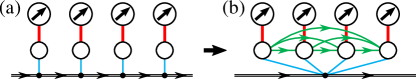
((a))

((b))

FIG. 1: (a) The impurities are Kondo-coupled to “buffer” dangling sites, which in turn quadratically couple to the chiral channels, and are considered part of the noninteracting bath. (b) Taking the distance between these sites to zero leads to an effective chiral model, in which the dangling sites together with the impurities form a large effective impurity.

We start with $M$ spin-$\frac{1}{2}$ impurities with spin operator $\mathbf{S}_{m}$ where $m\in\left\{1,...,M\right\}$, and a bath of right-moving free fermions

$$H_{\mathrm{chiral}} =\sum_{\alpha\sigma}\int dx\psi_{\alpha\sigma}^{\dagger}\left(x\right)\left(-iv_{F}\partial_{x}\right)\psi_{\alpha\sigma}\left(x\right),$$ (1)

with Fermi velocity $v_{F}$, spin $\sigma\in\left\{\uparrow,\downarrow\right\}$, and channel $\alpha\in\left\{1,..,k\right\}$. One can directly couple the impurities to the bath at locations $\left\{R_{m}\right\}$ by writing the Hamiltonian $\sum_{m}J\mathbf{S}_{m}\cdot\mathbf{s}\left(R_{m}\right)+H_{\mathrm{chiral}}$, with $J>0$ the Kondo coupling and $\mathbf{s}\left(x\right)\equiv\sum_{\alpha\sigma}\psi_{\alpha\sigma}^{\dagger}\left(x\right)\bm{{\sigma}}_{\sigma\sigma^{\prime}}\psi_{\alpha\sigma^{\prime}}\left(x\right)$ the bath spin at location $x$. We treat such a model in Ref. [31] by introducing $M$ coupled effective $k$-channel baths, but this comes with a very high computational price tag, due to the exponential scaling of NRG with the number of channels. Instead, here we employ a mapping which captures the chirality with a single $k$-channel bath. We first separate the impurities from the bath, as illustrated in Fig. 1(a), by introducing buffer “dangling” fermionic sites coupled to the bath at locations $\left\{R_{m}\right\}$, and then couple the impurities to these dangling sites, arriving at

$$H_{\mathrm{total}} =J\sum_{m}\mathbf{S}_{m}\cdot\mathbf{s}_{m}+H_{\mathrm{dang}}+H_{\mathrm{chiral}},$$ (2)

$$H_{\mathrm{dang}} =\tilde{t}_{0}\!\sum_{m\alpha\sigma}\!\left[d_{m\alpha\sigma}^{\dagger}\psi_{\alpha\sigma}\!\left(R_{m}\right)\!+\psi_{\alpha\sigma}^{\dagger}\!\left(R_{m}\right)\!d_{m\alpha\sigma}\right],$$ (3)

where $d_{m\alpha\sigma}$ and $\mathbf{s}_{m}\equiv\sum_{\alpha\sigma}d_{m\alpha\sigma}^{\dagger}\bm{{\sigma}}_{\sigma\sigma^{\prime}}d_{m\alpha\sigma^{\prime}}$ are the dangling-site fermionic and spin operators, respectively, $J>0$ is the Kondo coupling, and $\tilde{t}_{0}$ together with the Fermi velocity define a soft cutoff $\Gamma\equiv\frac{\tilde{t}_{0}^{2}}{2v_{F}}$.

Initially we treat the dangling sites together with the chiral channels as the noninteracting bath to which the impurities are coupled. As typical of Kondo problems, the bath dependence of impurity quantities enters (to all orders in the Kondo coupling $J$) only through the (retarded) Green function of the bath at the sites coupled to the impurities, i.e., the dangling sites, when these are decoupled from the impurities:

$$\mathbf{g}_{\mathrm{dang}}^{R}\left(\omega\right)=\left[\omega\mathbb{1}-\mathbf{h}-\mathbf{\Sigma}^{R}\left(\omega\right)\right]^{-1},$$ (4)

with $\mathbb{1}$ the $M{\times}M$ identity matrix, $\mathbf{h}{=}0$ the single-particle Hamiltonian acting on the dangling sites, and

$$\mathbf{\Sigma}_{mm^{\prime}}^{R}\left(\omega\right)=-2i\Gamma\Theta\left(R_{m^{\prime}}-R_{m}\right)e^{i\omega\left(R_{m^{\prime}}-R_{m}\right)/v_{F}},$$ (5)

the retarded self-energy due to the coupling of the dangling sites to the chiral channels, where $\Theta\left(x\right)$ is the Heaviside step function [taking $\Theta\left(0\right)=\frac{1}{2}$]. A clear signature of chirality (assuming right movers) is that any retarded quantity at location $r$ due to an event at $r^{\prime}>r$ vanishes. And indeed, all elements below the diagonal of $\mathbf{\Sigma}^{R}\left(\omega\right)$ are zero, as a result of which the same holds for $\mathbf{g}_{\mathrm{dang}}^{R}\left(\omega\right)$. Thus, importantly, the introduction of the dangling sites retains chirality. The obtained model is formally equivalent to one without dangling sites in the $\Gamma\to\infty$ limit, whereas for finite $\Gamma$ we have merely modified the bath density of states to a Lorentzian of width $\Gamma$ at each dangling site, which should not affect the universal low-energy properties. Assuming $J<\Gamma$, we can define the Kondo temperature as $T_{K}=\Gamma e^{-\pi\Gamma/J}$.

We now take the limit $\omega\!\left(R_{M}{-}R_{1}\right)\!/v_{F}\to 0$, corresponding to low temperatures or long wavelengths. This limit is taken after the infinite bandwidth limit of Eq. (1), and is not impaired by the soft cutoff $\Gamma$. $\mathbf{\Sigma}^{R}\left(\omega\right)$ loses its frequency dependence, but not its chirality, and can be written as

$$\mathbf{\Sigma}_{mm^{\prime}}^{R}\to-i\Gamma\!\left\{\!\!\begin{smallmatrix}2&m^{\prime}>m\\ 1&m^{\prime}=m\\ 0&m^{\prime}<m\end{smallmatrix}\right.\equiv\mathbf{h}_{mm^{\prime}}^{\mathrm{eff}}-i\Gamma,$$ (6)

with $\mathbf{h}^{\mathrm{eff}}$ a Hermitian matrix. Thus, $\mathbf{h}^{\mathrm{eff}}$ can be interpreted as an effective (single-particle) Hamiltonian coupling all dangling sites to each other via imaginary hopping amplitudes, while $-i\Gamma$ describes a single trivial bath coupled equally to all dangling sites, i.e.,

$$H_{\mathrm{dang}}^{\mathrm{eff}} =\sum_{\alpha\sigma}\sum_{m>m^{\prime}}it_{mm^{\prime}}^{\prime}\left[d_{m\alpha\sigma}^{\dagger}d_{m^{\prime}\alpha\sigma}-d_{m^{\prime}\alpha\sigma}^{\dagger}d_{m\alpha\sigma}\right]$$

$$+\sqrt{M}\tilde{t}_{0}\sum_{m\alpha\sigma}\left[d_{m\alpha\sigma}^{\dagger}\psi_{\alpha\sigma}\!\left(0\right)\!+\psi_{\alpha\sigma}^{\dagger}\!\left(0\right)\!d_{m\alpha\sigma}\right],$$ (7)

with $t_{mm^{\prime}}^{\prime}=\Gamma$. Replacing $H_{\mathrm{dang}}$ in Eq. (2) with $H_{\mathrm{dang}}^{\mathrm{eff}}$, we arrive at the model depicted in Fig. 1(b).

Let us review what we have achieved. The obtained model is still chiral (for the very specific choice of $t_{mm^{\prime}}^{\prime})$, and reproduces the bath Green function in the low temperature limit. But now we can interpret the impurities together with the dangling sites as a large effective impurity, coupled to an effective bath (described only by $H_{\mathrm{chiral}}$) at a single location, so that its chirality is no longer important. The resulting structure also hints at first fusing all the impurities together, and then fusing onto a single (multichannel) bath, as in the CFT ansatz of Ref. [27]. The obtained model is amendable to standard NRG, although one still needs to account for the multiple channels. In order to reduce the computational cost, we exploit the different symmetries of the model (charge, spin, channel), using the QSpace tensor network library, which treats Abelian and non-Abelian symmetries on equal footing [33, 34, 35]. For implementation details see Sec. III in the Supplemental Material [28] and Refs. [36, 37, 38, 39] therein. In order to apply NRG, we introduce an artificial sharp high-energy cutoff $D\gg\Gamma,J$ to the bath density of states. This cutoff, and to a lesser extent the NRG discretization and truncation, mimic the effect of the bulk bands (Landau levels), setting a finite bandwidth for the chiral edge mode, and mediating effective nonchiral RKKY interactions between the impurities. The latter are expected to decay exponentially with both the bulk gap and the interimpurity distance [40, 41, 42], and are thus eliminated by numerically tuning each $t_{mm^{\prime}}^{\prime}$ slightly away from $\Gamma$ to reinstate chirality (see Sec. IV.4 in the Supplemental Material [28]).

Results.—

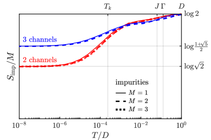
FIG. 2: Impurity entropy per impurity for two channels (red) with 1–3 impurities, and three channels (blue) with 1–2 impurities, taking $2J{=}\Gamma{=}D/8$. At high temperatures the impurity spins are free, each contributing an entropy of $\log 2$. At low temperatures each impurity contributes a fractional entropy corresponding to the quantum dimension of Ising [$\mathrm{SU}\!\left(2\right)_{2}$] or Fibonacci [$\mathrm{SU}\!\left(2\right)_{3}$] anyons for two or three channels, respectively.

We apply NRG to the effective Hamiltonian for two channels with up to three impurities, and for three channels with up to two impurities. In Fig. 2 we plot the impurity entropy $S_{\mathrm{imp}}$, defined as the difference between the entropy of the full system and that of the fermionic bath (dangling sites + chiral channels) in the absence of the impurities, which quantifies the effective degree of freedom $d_{\mathrm{eff}}$ each impurity introduces. We find that $d_{\mathrm{eff}}$ is independent of the number of impurities $M$, so that $S_{\mathrm{imp}}/M=\log d_{\mathrm{eff}}\left(k,T\right)$ follows the universal single-impurity curve, matching the limit of infinitely separated impurities, and thus supporting our argument that in a chiral system the interimpurity distance is not important. At high temperatures each impurity is effectively a free spin, contributing a $d_{\mathrm{eff}}{=}2$ degree of freedom. Going below the Kondo temperature while assuming the thermodynamic limit for the bath, each impurity contributes a fractional degree of freedom $d_{\mathrm{eff}}{=}d_{k}$ corresponding exactly to an $\mathrm{SU}\!\left(2\right)_{k}$ anyon. These results are well known in the single-impurity scenario [20], but the scaling to multiple impurities, implying an anyon for each impurity, is quite remarkable. This is very different from the paradigmatic multi-impurity multichannel scenario, where the initially similar entropy curves break for temperatures below $\sim v_{F}/R$ due to coherent backscattering which generates effective RKKY interactions. In order to probe anyonic statistics we need coherence, and indeed in our case we are already in the regime of $T\ll v_{F}/R\to\infty$, but now due to chirality, backscattering is forbidden, and the anyons survive.

The curves in Fig. 2 were obtained for the specific choice of the dangling-site hopping amplitudes $t_{mm^{\prime}}^{\prime}$ which renders the system chiral. We can characterize this point by artificially tuning away from it, and demonstrate that at the chiral point, the low-energy theory is exactly that of the CFT ansatz of Ref. [27]. This is best observed in the finite-size spectrum obtained by NRG, but as its analysis is quite technical, we defer it to Sec. II in the Supplemental Material [28]. Instead, here we discuss more intuitive quantities.

For two impurities, with either two or three channels, we find that the effective system undergoes a quantum phase transition from a Kondo-screened spin-1 impurity when the single parameter $t_{12}^{\prime}$ is below some critical value to a spin-0 “Kondo” effect above it, similar to the two-impurity Kondo-RKKY phase transition [43]. The two phases can be identified by their low-energy spectra (see Sec. II in the Supplemental Material [28]), with the transition observed, e.g., in the interimpurity spin correlator $\left\langle\mathbf{S}_{1}\!\cdot\mathbf{S}_{2}\right\rangle_{T\to 0}$, which flips sign from positive (tripletlike) to negative (singletlike), as shown in Fig. 3(a). Tuning away from criticality and projecting the operator $\mathbf{S}_{1}\!\cdot\mathbf{S}_{2}$ down to the low-energy subspace, we find it is a constant (equal to $\left\langle\mathbf{S}_{1}\!\cdot\mathbf{S}_{2}\right\rangle_{T\to 0}$), and thus commutes with the low-energy Hamiltonian. This is consistent with our characterization of the two phases, but is not trivial, as $\mathbf{S}_{1}\!\cdot\mathbf{S}_{2}$ does not commute with the full Hamiltonian, and hence the definite spin states (singlet and triplet) mix low- and high-energy states. The critical $t_{12}^{\prime}$ is exactly the hopping amplitude required for the system to be chiral (it indeed converges to $\Gamma$ for $D\gg\Gamma,J$; see Fig. S4(a) in the Supplemental Material [28]). The projected $\mathbf{S}_{1}\!\cdot\mathbf{S}_{2}$ also commutes with the low-energy Hamiltonian at this point, but now has two eigenvalues, positive and negative. Projecting onto the subspace corresponding to the negative (positive) eigenvalue takes us back to the spin-0 (spin-1) Kondo phase. Thus, at the chiral point, the low-energy Hamiltonian is the direct sum of the low-energy Hamiltonians of the spin-0 and spin-1 Kondo effects. Remembering these can be obtained by fusing an $\mathrm{SU}\!\left(2\right)_{k}$ charge-0 or 1 anyon to the $k$-channel bath, we see that in the chiral case we fuse two charge-$\frac{1}{2}$ anyons to the bath

$$0\times\mathrm{Bath}+1\times\mathrm{Bath}=\left(0+1\right)\times\mathrm{Bath}=\tfrac{1}{2}\times\tfrac{1}{2}\times\mathrm{Bath},$$

in perfect agreement with the CFT ansatz of Ref. [27]. As a byproduct we have also demonstrated that a (low-energy) measurement of the spin correlator $\mathbf{S}_{1}\!\cdot\mathbf{S}_{2}$ actually measures the fusion outcome of the two anyons. We note that this relation between the fusion channel and the spin correlator was also recently demonstrated analytically in the limits of $k{=}2$ and large-$k$ channels [44].

This suggests we can extract the anyonic $F$ matrix, which fully characterizes the non-Abelian part of the anyonic theory [3], from measurements of different pairwise spin correlators, as depicted in Fig. 3(b). We explicitly demonstrate this for three impurities and two channels. We now tune two parameters: the nearest-neighbor $t_{12}^{\prime}=t_{23}^{\prime}$ (equal by symmetry) and next-nearest-neighbor $t_{13}^{\prime}$ hopping amplitudes. For general values the effective low-energy Hamiltonian is that of a single spin-$\frac{1}{2}$ two-channel Kondo (2CK) effect, $H_{\mathrm{2CK}}$. However, at a single critical point, corresponding to the system being chiral, we get a twofold degeneracy (for each energy eigenstate) on top of this 2CK effect. We can thus write the low-energy Hamiltonian as a direct sum of two 2CK low-energy Hamiltonians $H_{\mathrm{2CK}}{\oplus}H_{\mathrm{2CK}}$, each given by CFT by fusing a charge-$\frac{1}{2}$ anyon to the bath

$$\left(\tfrac{1}{2}+\tfrac{1}{2}\right)\times\mathrm{Bath}=\tfrac{1}{2}\times\left(0+1\right)\times\mathrm{Bath}=\tfrac{1}{2}\times\tfrac{1}{2}\times\tfrac{1}{2}\times\mathrm{Bath}.$$

This is equivalent to fusing three charge-$\frac{1}{2}$ anyons to the bath, again in perfect agreement with the CFT ansatz of Ref. [27]. We see that the degeneracy is associated to a decoupled fusion space, and can write the low-energy Hamiltonian as an outer product $H_{\mathrm{2CK}}{\otimes}\mathbb{1}_{2\times 2}$, acting on the “energy space” and (trivially) on the fusion space.

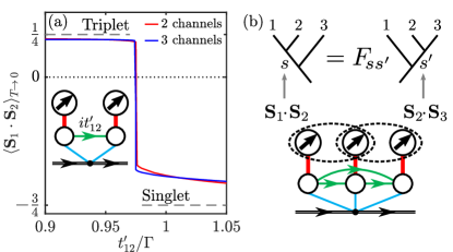
((a))

((b))

FIG. 3: (a) Quantum phase transition for two impurities with two (red) and three (blue) channels as a function of the dangling-site hopping amplitude $t_{12}^{\prime}$, taking $2J{=}\Gamma{=}D/8$. Correlations for the bare singlet and triplet are indicated by dashed lines. (b) Extraction of the $F$ matrix from interimpurity spin correlators in a three-impurity system.

Projecting the three pairwise spin correlators $\mathbf{S}_{1}\negmedspace\cdot\mathbf{S}_{2}$, $\mathbf{S}_{2}\negmedspace\cdot\mathbf{S}_{3}$, and $\mathbf{S}_{1}\negmedspace\cdot\mathbf{S}_{3}$ down to the low-energy subspace, we find all three commute with the low-energy Hamiltonian, and act nontrivially only on the fusion space. Thus, for each pair of impurities $m,m^{\prime}$ the projected $\mathbf{S}_{m}\negmedspace\cdot\mathbf{S}_{m^{\prime}}$ can be written as $\mathbb{1}_{\mathrm{2CK}}\otimes\mathbf{s}_{mm^{\prime}}$, where $\mathbb{1}_{\mathrm{2CK}}$ is the identity matrix in the “energy space” and $\mathbf{s}_{mm^{\prime}}$ is a $2{\times}2$ Hermitian matrix. Diagonalizing $\mathbf{s}_{mm^{\prime}}$ we find that it (and thus $\mathbf{S}_{m}\negmedspace\cdot\mathbf{S}_{m^{\prime}}$) has one negative (singletlike) and one positive (tripletlike) eigenvalue, with eigenstates $\Ket{0_{mm^{\prime}}}$ and $\Ket{1_{mm^{\prime}}}$, respectively. The different correlators do not commute with each other, and so define different bases for the fusion space, related by the basis transformation

$$\!F\,{=}\begin{pmatrix}\Braket{0_{12}}{0_{23}}&\Braket{0_{12}}{1_{23}}\\ \Braket{1_{12}}{0_{23}}&\Braket{1_{12}}{1_{23}}\end{pmatrix}{=}\frac{1}{\sqrt{2}}\!\begin{pmatrix}1.003&0.997\\ 0.997&-1.003\end{pmatrix}\!.$$ (8)

For concreteness we have restricted ourselves to the relation between the eigenbases of $\mathbf{S}_{1}\negmedspace\cdot\mathbf{S}_{2}$ and $\mathbf{S}_{2}\negmedspace\cdot\mathbf{S}_{3}$, and presented the numerically extracted values in this case. We note that this result displays dependence on the ratio $J/\Gamma$, which we discuss in Sec. IV of the Supplemental Material [28]. Interpreting the eigenstates of the spin correlator $\mathbf{S}_{m}\negmedspace\cdot\mathbf{S}_{m^{\prime}}$ as states with definite fusion outcomes of anyons $m$ and $m^{\prime}$ (as in the two-impurity case), Eq. (8) exactly defines the $F$ matrix, which matches $\frac{1}{\sqrt{2}}\!\!\left(\begin{smallmatrix}1&1\\ 1&-1\end{smallmatrix}\!\right)$ corresponding to $\mathrm{SU}\!\left(2\right)_{2}$ anyons.

Conclusions.—

We have numerically demonstrated that multiple Kondo impurities coupled to $k$ chiral channels (i) host multiple $\mathrm{SU}\!\left(2\right)_{k}$ non-Abelian anyons (one per impurity), highlighted by the fractional entropy contribution per impurity, and (ii) the emergence of a decoupled fusion space, which can be probed by low-energy measurements of the interimpurity spin correlators, explicitly extracting the $F$ matrix of $\mathrm{SU}\!\left(2\right)_{2}$ anyons. The anyons can now be braided by a measurement-only protocol [29], which teleports them using only measurements of pairwise topological charge (fusion channel). One can envision implementing this protocol, e.g., by a low-energy scattering experiment, directly demonstrating the non-Abelian nature of the anyons in the system.

Experiments consisting of a single impurity coupled to two and three integer quantum Hall edge states (i.e., chiral channels) have already been carried out [18, 19], with clear signatures of the fractionalized degrees of freedom [45, 46, 47, 48]. Extending these experiments to multiple impurities with all spin and channel species propagating between the impurities is a challenge. Testing if more realistic setups, in which only some of the species connect the impurities while the remainder are local to each impurity, also support non-Abelian anyons, and what physical observables probe their fusion space, is quite straightforward for the method presented, and is left for future work. Note that due to the absence of a (topological) gap, we expect information encoded in the fusion space to decohere as a power law of $T/T_{K}$, in contrast to the exponential suppression in the presence of a gap. Still, based on the success of Refs. [18, 19], the path to observing non-Abelian anyons might be shorter in these systems.

Supplemental Material for
“Manipulating Non-Abelian Anyons in a Chiral Multichannel Kondo Model”

This supplemental consists of four sections. Sec. I shortly reviews relevant results and implications of the multi-impurity CFT ansatz of Lopes et al. [27], and specifically the resulting finite-size spectrum. In Sec. II we analyze the NRG low-energy spectrum and demonstrate its agreement with the CFT ansatz finite-size spectrum. Sec. III contains NRG implementation instructions followed by a discussion of the model symmetries and how to exploit them. Finally, in Sec. IV we discuss the model and NRG parameters used throughout.

I Implications of the CFT Ansatz

Affleck and Ludwig [21] conjectured (and then demonstrated by comparing to both analytical and numerical solutions) that the low-energy physics of the single spin-$s$ impurity $k$-channel Kondo effect is captured by a boundary CFT in which a single $\mathrm{SU}\!\left(2\right)_{k}$ “anyon” with “topological” charge $s$ is fused to the primary fields of $k$ channels of free fermions. Here “anyons” of charge $s$ are in one to one correspondence with the primary field of the $\mathrm{SU}\!\left(2\right)_{k}$ Wess-Zumino-Witten theory, labeled by $s=0,\frac{1}{2},1,...,\frac{k}{2}$, and satisfying the fusion rules given in Eq. (S1) below. Generalizing upon this, Lopes et al. [27] conjectured that for $M$ spin-$s$ impurities, and assuming the $k$ channels are chiral, the low-energy physics is captured by fusing $M$ such $\mathrm{SU}\!\left(2\right)_{k}$ anyons, each with charge $s$, to the primary fields of $k$ channels of free fermions. Here we will outline some of the consequences of this conjecture for two examples: $M$ spin-$\frac{1}{2}$ impurities with $k=2$ or $k=3$ channels.

$\begin{array}[]{lcc}\qquad\text{$\mathrm{SU\!\left(2\right)_{2}}$ Anyons}&\!\!\!\!\!\!\!\!\longrightarrow&\text{Ising Anyons (Majoranas)}\\ \begin{array}[]{l}0\times s=s\ ;\ s\in\left\{0,\tfrac{1}{2},1\right\}\\ \!\tfrac{1}{2}\times\tfrac{1}{2}=0+1\\ \!\tfrac{1}{2}\times 1=\tfrac{1}{2}\\ 1\times 1=0\end{array}&\!\!\!\!\!\!\!\!\longrightarrow&\begin{array}[]{l}\mathbf{1}\times\alpha=\alpha\ ;\ \alpha\in\left\{\mathbf{1},\sigma,\psi\right\}\\ \sigma\times\sigma=\mathbf{1}+\sigma\\ \sigma\times\psi=\sigma\\ \psi\times\psi=\mathbf{1}\end{array}\\ &\vspace{-1em}\hfil\end{array}$

$\begin{array}[]{lcc}\quad\qquad\text{$\mathrm{SU\!\left(2\right)_{3}}$ Anyons}&\!\!\!\!\!\!\!\!\!\!\!\!\longrightarrow&\text{Fibonacci Anyons}\\ \begin{array}[]{l}\!\!\begin{array}[]{l}0\times s=s\\ \!\tfrac{3}{2}\times s=\tfrac{3}{2}-s\end{array};\ s\in\left\{0,\tfrac{1}{2},1,\tfrac{3}{2}\right\}\\ \!\tfrac{1}{2}\times\tfrac{1}{2}=1\times 1=0+1\\ \!\tfrac{1}{2}\times 1=\tfrac{1}{2}+\tfrac{3}{2}\end{array}&\!\!\!\!\!\!\!\!\!\!\!\!\longrightarrow&\begin{array}[]{l}\mathbf{1}\times\alpha=\alpha\ ;\ \alpha\in\left\{\mathbf{1},\tau\right\}\\ \\ \tau\times\tau=\mathbf{1}+\tau\end{array}\\ &\vspace{-1em}\hfil\end{array}$

TABLE. SI: Fusion rules for different anyonic models. For $\mathrm{SU}\!\left(2\right)_{2}$ anyons we can associate the topological charges $\left\{0,\frac{1}{2},1\right\}$ with the vacuum $\mathbf{1}$, a Majorana fermion $\sigma$, and an occupied Dirac fermion $\psi$, respectively, arriving at the fusion rules of Ising anyons. For $\mathrm{SU}\!\left(2\right)_{3}$ anyons we associate both $0$ and $\frac{3}{2}$ with the vacuum $\mathbf{1}$, and both $\frac{1}{2}$ and $1$ with the $\tau$ anyon, arriving at the fusion rules of Fibonacci anyons.

The fusion rule of two $\mathrm{SU}\!\left(2\right)_{k}$ anyons with topological charges $s_{1},s_{2}\leq\frac{k}{2}$ is given by

$$s_{1}\times s_{2}=\left|s_{1}-s_{2}\right|+\left(\left|s_{1}-s_{2}\right|+1\right)+...+\min\left(s_{1}+s_{2},k-s_{1}-s_{2}\right),$$ (S1)

which for $k\to\infty$ is simply the standard $\mathrm{SU}\!\left(2\right)$ fusion rule, i.e., the angular momentum addition rule. Specifically for $k=2$ and $k=3$ we get the fusion rules in Table SI, which can be identified with those of Ising and Fibonacci anyons, respectively (see caption). Fusing $M$ charge-$\frac{1}{2}$ anyons according to these rules we get

$$\mathrm{SU\!\left(2\right)_{2}}:\quad\overset{M}{\overbrace{\tfrac{1}{2}\times\tfrac{1}{2}\times...\times\tfrac{1}{2}}} =\Biggl{\{}\begin{array}[]{ll}\overset{2^{\left(M-1\right)/2}}{\overbrace{\tfrac{1}{2}+\tfrac{1}{2}+...+\tfrac{1}{2}}}&\text{odd }M\\ \underset{2^{M/2-1}}{\underbrace{0+...+0}}+\underset{2^{M/2-1}}{\underbrace{1+...+1}}&\text{even }M\end{array},$$ (S4)

$$\mathrm{SU\!\left(2\right)_{3}:\quad\overset{M}{\overbrace{\tfrac{1}{2}\times\tfrac{1}{2}\times...\times\tfrac{1}{2}}}} =\Biggl{\{}\begin{array}[]{ll}\overset{F_{M}}{\overbrace{\tfrac{1}{2}+...+\tfrac{1}{2}}}+\overset{F_{M-1}}{\overbrace{\tfrac{3}{2}+...+\tfrac{3}{2}}}&\text{odd }M\\ \underset{F_{M-1}}{\underbrace{0+...+0}}+\underset{F_{M}}{\underbrace{1+...+1}}&\text{even }M\end{array},$$ (S7)

where $F_{M}$ are the elements of the Fibonacci sequence $F_{0}=0,F_{1}=1,F_{M>1}=F_{M-1}+F_{M-2}$. Projecting onto any specific fusion outcome, we get a (fusion) Hilbert space which grows exponentially with the number of anyons. For $k=2$, adding two anyons doubles the size of the fusion space, and so a single anyon carries a quantum dimension of $\sqrt{2}$. For $k=3$ we see that it make sense to associate both $\frac{1}{2}$ and $1$ with the $\tau$ anyon and $0$ and $\frac{3}{2}$ with the vacuum (as in Table SI), and then adding a single $\tau$ anyon enlarges the dimension of the fusion space by $F_{M}/F_{M-1}$, which in the large $M$ limit gives the golden ratio $\frac{1+\sqrt{5}}{2}$, i.e., the quantum dimension associated with Fibonacci anyons.

Returning to the multi-impurity fusion ansatz we note that due to the associativity of fusion, we can first fuse the $M$ charge-$\frac{1}{2}$ anyons to each other, arriving at the anyonic fusion space of Eq. (S4) or (S7), and then fuse this space onto the free fermions. In order to calculate the spectrum, we simply need to solve for single spin-$s=\frac{1}{2},1,...,\frac{k}{2}$ impurities coupled to $k$ channels, and add the degeneracies according to the fusion outcomes by hand. In Sec. II we will demonstrate that the low-energy spectrum obtained from NRG (for two impurities with two and three channels, and for three impurities with two channels) exactly matches this structure.

II Finite-Size Spectrum

((a))

((b))

((c))

FIG. S1: NRG low-energy spectrum at the chiral point, i.e., critical hopping $t_{c}^{\prime}$ (gray), and away from it (red and blue). The chiral spectrum agrees with the $\mathrm{SU}\!\left(2\right)_{k}$ CFT finite-size spectrum for $k$ channels and different number of impurities (anyons). (a,b) For two spin-$\frac{1}{2}$ impurities it is given by overlaying the spectrum of a spin-0 (blue) and spin-1 (red) $k$-channel Kondo spectrum, while (c) for three impurities it is given by two identical copies of the spin-$\frac{1}{2}$ $k$-channel Kondo spectrum (red). Observe that the degeneracies (black text), which for the chiral spectrum (gray) are partitioned according to the expectation values of the spin correlator, indeed match those of the corresponding fusion channel. NRG parameters $\Lambda=2$ for (a,b) and $\Lambda=3$ for (c), $N_{K}=4000$, and model parameters $J=\Gamma=8D$ are chosen for optimal numerical convergence, as discussed in Sec. IV.

In this section we study the effective Hamiltonian at the low-energy fixed point, as obtained by NRG. As the system is gapless, in the thermodynamic limit it has a continuous spectrum, but at any given NRG iteration we can interpret the spectrum as that of a finite system, in which case we do have discrete levels. One needs to choose the boundary conditions of this finite system, and they dictate whether the bath has an even or odd number of single-particle modes. For conciseness, we will restrict our discussion to an even number of such modes, corresponding to even NRG iterations, and to half filling, so that there is no single-particle level at the Fermi energy. As we exploit the global symmetries of the model as part of the NRG procedure, we retain the information regarding the quantum numbers, i.e., symmetry labels, of each one of the many-body levels in the low-energy spectrum. We will now demonstrate that the obtained spectrum is in perfect agreement with the finite-size spectrum of the boundary CFT ansatz of Ref. [27], which is obtained by $\mathrm{SU}\!\left(2\right)_{k}$ fusion rules as outlined in Sec. I.

II.1 Two Impurities

We start with two impurities and two or three channels. By setting $t_{12}^{\prime}$, the hopping amplitude between the dangling sites, to be above (below) the critical (chiral) value $t_{c}^{\prime}$, we get the low-energy fixed-point spectra of a single spin-0 (spin-1) impurity Kondo effect, as plotted in blue (red) in Figs. S1(a) and S1(b), for two and three channels respectively. These can be calculated, e.g., via boundary CFT [21] by fusing an $\mathrm{SU}\!\left(2\right)_{k}$ anyon of charge-$s$ to the primary fields of ($k$-channel) free fermions. For $s=0$ this simply leaves us with $k$ channels of free fermions, which can easily be verified. For spin-1 and two channels, each channel contributes a single spin-$\frac{1}{2}$ fermion, thus fully screening the impurity, and resulting in a $\frac{\pi}{2}$ phase shift, i.e., free fermions with an odd number of single particle modes (assuming we started with an even number of modes). For spin-1 and three channels we get an over-screened effect, which results in a non-fermi liquid. Tuning to the critical point, we find that there is no hybridization between the energy levels of the two spectra, which are simply overlayed, as demonstrated in gray in Figs. S1(a) and S1(b). This is exactly the picture one expects when fusing two charge-$\frac{1}{2}$ anyons to a $k$-channel bath:

$$\tfrac{1}{2}\times\tfrac{1}{2}\times\mathrm{Bath}=\left(0+1\right)\times\mathrm{Bath}=0\times\mathrm{Bath}+1\times\mathrm{Bath},$$

or in words, we first fuse the two anyons to each other, resulting in an anyonic charge of either 0 or 1, which is then separately fused to the bath, arriving at the combined spectrum. Thus, we understand that levels associated with the different spectra belong to different fusion channels, which explains the absence of hybridization. For two impurities, most levels in the combined spectrum are associated either with only one of the fused charges, as is, e.g., the case for the many-body ground state. However, we do have levels which are associated with both channels, e.g., the first (second) excited level for $k=2$ ($k=3$) channels, in which case we observe anyonic degeneracy.

As discussed in the main text, projecting the interimpurity spin correlator $\mathbf{S}_{1}\!\cdot\mathbf{S}_{2}$ onto the low-energy subspace results in an operator which commutes with the low-energy Hamiltonian, and so we can mutually diagonalize them. The low-energy projected $\mathbf{S}_{1}\!\cdot\mathbf{S}_{2}$ has only two distinct eigenvalues, one negative (singletlike) and one positive (tripletlike). Calculating the relevant eigenvalue for each level in the spectra in Figs. S1(a) and S1(b), we indicate in blue (red) the degeneracies of the levels with the negative (positive) eigenvalue, and find that they exactly match those associated with the spin-0 (spin-1) spectrum. We thus establish that $\mathbf{S}_{1}\!\cdot\mathbf{S}_{2}$ indeed measures the fusion outcome. Note that away from the critical point, only one fusion outcome survives, and indeed the low-energy projected $\mathbf{S}_{1}\!\cdot\mathbf{S}_{2}$ is proportional to the identity in these cases.

We point out that due to the NRG discretization, we expect (and observe) corrections (with respect to the CFT spectra), i.e., splitting and shifting of energy levels, which become more pronounced at higher energy levels. However, these corrections affect the spectra in a systematic manner without breaking the correspondence between the spectrum at the critical point and the spectra of the two phase away from it. Still, for a clear comparison we choose the model parameters as discussed in Sec. IV.

II.2 Three Impurities

Going to three impurities and two channels, we have three imaginary hopping amplitudes which we need to tune. The nearest-neighbor terms $t_{12}^{\prime}$ and $t_{23}^{\prime}$ are equal by (time reversal + inversion) symmetry, while the next-nearest-neighbor term $t_{13}^{\prime}$ can have a different value. In the absence of the artificial cutoff $D$ all three should be equal to $\Gamma$, which implies a single critical point in a two-dimensional parameter space. As in the two-impurity case, we expect any deviation from this critical point to send us to one of the two fusion outcomes. However, in the case of three impurities and two channels we have

$$\tfrac{1}{2}\times\tfrac{1}{2}\times\tfrac{1}{2}\times\mathrm{Bath}=\left(\tfrac{1}{2}+\tfrac{1}{2}\right)\times\mathrm{Bath}=\tfrac{1}{2}\times\mathrm{Bath}+\tfrac{1}{2}\times\mathrm{Bath},$$

so that the two fusion outcomes correspond to identical phases, i.e., a single-impurity 2CK low-energy spectra, as shown in red in Fig. S1(c). Still, they do differ in their fusion path, e.g., in the fusion outcome of the first two impurities, and indeed we find that the interimpurity spin correlator $\mathbf{S}_{1}\!\cdot\mathbf{S}_{2}$ has two distinct regimes (the same holds for $\mathbf{S}_{1}\!\cdot\mathbf{S}_{3}$, and trivially by symmetry for $\mathbf{S}_{2}\!\cdot\mathbf{S}_{3}$). Generally the crossover between these two regimes is smooth, with only a single point of discontinuity. Tuning exactly to this point, we get the spectrum of three spin-$\frac{1}{2}$ impurities fused to two-channel bath, as shown in gray in Fig. S1(c). We can again count the levels associated with each of the eigenvalues of $\mathbf{S}_{1}\!\cdot\mathbf{S}_{2}$ (or $\mathbf{S}_{2}\!\cdot\mathbf{S}_{3}$ or $\mathbf{S}_{1}\!\cdot\mathbf{S}_{3}$) and indeed we find that for each level with the positive eigenvalue we have one with the negative eigenvalue.

III NRG Implementation Details

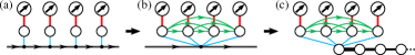
((a))

((b))

((c))

FIG. S2: Mapping of (a) the original dangling-site model to (b) the effective model in the limit of very close impurities, and then (c) after replacing the trivial bath by a Wilson chain as in Eq. (S9).

Here we will outline the technical details of applying NRG to our effective model. We assume familiarity with the NRG jargon, and stop short of reviewing the iterative diagonalization, which can be carried out by a traditional [36] or contemporary (tensor-network based) [33] implementation. We will start by discussing the mapping to a Wilson chain (although this is standard procedure), and follow with a discussion about exploiting symmetries of the problem.

III.1 Mapping to a Wilson Chain

Our starting point is the Hamiltonian in Eq. (2), depicted in Fig. S2(a). After replacing $H_{\mathrm{dang}}$ with $H_{\mathrm{dang}}^{\mathrm{eff}}$ of Eq. (7), we arrive at the effective Hamiltonian depicted in Fig. S2(b), which describes a large effective impurity consisting of the original impurity spins together with the dangling sites (and the imaginary couplings between them, which encode the chirality), coupled to a trivial bath given by $H_{\mathrm{chiral}}$ of Eq. (1). It is straightforward to diagonalize the bath by going to $k$-space

$$H_{\mathrm{chiral}}=\sum_{\alpha\sigma}\int_{-\infty}^{\infty}\frac{dk}{2\pi}v_{F}kc_{k\alpha\sigma}^{\dagger}c_{k\alpha\sigma},\quad c_{k\alpha\sigma}=\int_{-\infty}^{\infty}dxe^{-ikx}\psi_{\alpha\sigma}\left(x\right).$$ (S8)

We then introduce a sharp high-energy cutoff $v_{F}k_{\max}=D$ and logarithmically discretize [36, 37, 38] Eq. (S8). Tridiagonalizing the full (effective) Hamiltonian, we arrive at

$$H_{\mathrm{disc}} =J\sum_{m}\mathbf{S}_{m}\cdot\mathbf{s}_{m}+\sum_{\alpha\sigma}\sum_{m>m^{\prime}}it_{mm^{\prime}}^{\prime}\left(d_{m\alpha\sigma}^{\dagger}d_{m^{\prime}\alpha\sigma}-d_{m^{\prime}\alpha\sigma}^{\dagger}d_{m\alpha\sigma}\right)$$

$$+\sqrt{M}t_{0}\sum_{m\alpha\sigma}\left(d_{m\alpha\sigma}^{\dagger}c_{0\alpha\sigma}+c_{0\alpha\sigma}^{\dagger}d_{m\alpha\sigma}\right)+\sum_{\alpha\sigma}\sum_{n=0}^{N}t_{n}\left(c_{n\alpha\sigma}^{\dagger}c_{\left(n+1\right)\alpha\sigma}+c_{\left(n+1\right)\alpha\sigma}^{\dagger}c_{n\alpha\sigma}\right),$$ (S9)

with $t_{0}=\sqrt{\frac{2}{\pi}\Gamma D}$ and $t_{n}\sim D\Lambda^{-n/2}$ the exponentially decaying hopping amplitudes along the Wilson chain, which is of some finite length $N$. Thus, the effective impurity is now coupled to the first site of a standard Wilson chain, as depicted in Fig. S2(c). We then proceed to iteratively diagonalize this chain, adding one chain site at a time, diagonalizing the new Hamiltonian, and truncating to a fixed number $N_{K}$ of low-energy states. For each iteration we thus have an effective low-energy spectrum which we can analyze (see Sec. II), and from which can extract thermodynamic quantities, e.g., the impurity entropy, associated with a temperature $T\sim D\Lambda^{-n/2}$. We stop the iterative diagonalization, i.e., choose $N$, once we see that all quantities have converged.

III.2 Exploiting Symmetries

In order to reduce the computational cost of the iterative diagonalization procedure, we exploit global symmetries, which is quite natural when formulating NRG in terms of a tensor-network algorithm. In the case of Abelian symmetries, the tensors (or matrices) break down into a block structure, so that each block is diagonalized separately, thus allowing larger tensors, or a larger number of kept states $N_{K}$ in each iteration (for the same computational cost). The significant advantage comes from exploiting non-Abelian symmetries, in which case each block can be decomposed into an outer product of “actual information” (akin to reduced matrix elements in the Wigner-Eckart theorem [39]) and “symmetry structure”, with the later encoded in (generalized) Clebsch-Gordan coefficients [34]. We then need to only diagonalize the “actual information” part which significantly reduces the size of each block.

The symmetries typically associated with the multichannel Kondo problem are $\mathrm{SU\!\left(2\right)}$ spin symmetry (in the absence of a magnetic field), as well as $\mathrm{U\!\left(1\right)}$ charge (particle number) and $\mathrm{SU\!\left(k\right)}$ channel symmetries, or compactly, $\mathrm{U\!\left(1\right)_{charge}\times SU\!\left(k\right)_{channel}\times SU\!\left(2\right)_{spin}}$ symmetry. The CFT ansatz is formulated in terms of the these symmetries, and one can easily verify that both the original and effective discrete multi-impurity Hamiltonians in Eqs. (2) and (S9), respectively, conserve these symmetries. We also consider the system in a particle-hole symmetric regime, in which case the charge and channel symmetries are elevated to an $\mathrm{Sp\!\left(2k\right)}$ symmetry [34], so that the full symmetry of the model is actually $\mathrm{Sp\!\left(2k\right)_{\text{charge-channe}l}\times SU\!\left(2\right)_{spin}}$. This is a direct generalization of the more widely known $\mathrm{SU\!\left(2\right)_{charge}\times SU\!\left(2\right)_{spin}}$ symmetry in the single-channel case. We can actually stick to our intuition for the single-channel case, and resolve all arising complications at that level, with specific technical challenges for exploiting the $\mathrm{Sp\!\left(2k\right)}$ symmetry taken care at the level of the tensor-network library [34, 35].

We start by formulating the particle-hole transformation under which the Hamiltonian is invariant

$$\psi_{\alpha\sigma}\left(x\right)\leftrightarrow\psi_{\alpha\sigma}^{\dagger}\left(x\right)\ \Leftrightarrow\ c_{k\alpha\sigma}\leftrightarrow c_{-k\alpha\sigma}^{\dagger}\ \Leftrightarrow\ c_{n\alpha\sigma}\leftrightarrow\left(-1\right)^{n}c_{n\alpha\sigma}^{\dagger}\quad;\quad d_{m\alpha\sigma}\leftrightarrow-d_{m\alpha\sigma}^{\dagger}$$ (S10)

noting that this, together with the $\mathrm{U\!\left(1\right)_{charge}}$ symmetry suffices in to claim $\mathrm{SU\!\left(2\right)_{charge}}$ symmetry in the single-channel case (and $\mathrm{Sp\!\left(2k\right)}$ symmetry in the $\mathrm{SU\!\left(k\right)_{channel}}$ symmetric case). Observe that the dangling-site operators flip sign under the transformation, as do the odd sites in the Wilson chain. It is usually argued that under $\mathrm{SU\!\left(2\right)_{charge}}$ symmetry we can partition our tight-binding model into a bipartite graph (in our case even chain sites on the one side and odd chain sites together with the dangling sites on the other), allowing only (purely real) couplings which cross the partition. However, this restriction assume the system is invariant under time reversal $t\to-t$, while a chiral system is not, and is only invariant under time reversal together with inversion, $t\to-t,x\to-x$. In this case purely imaginary couplings between sites on the same side of the partition also respect the symmetry, e.g., as in the case of the dangling sites. On a technical level we note that if one can only implement (real) terms which cross the partition, e.g., $\sum_{\alpha\sigma}\left(d_{m\alpha\sigma}^{\dagger}c_{0\alpha\sigma}+c_{0\alpha\sigma}^{\dagger}d_{m\alpha\sigma}\right)$, one can still obtain the imaginary terms by calculating commutators

$$\sum_{\alpha\sigma}i\left(d_{m\alpha\sigma}^{\dagger}d_{m^{\prime}\alpha\sigma}-d_{m^{\prime}\alpha\sigma}^{\dagger}d_{m\alpha\sigma}\right)=i\left[\sum_{\alpha\sigma}\left(d_{m\alpha\sigma}^{\dagger}c_{0\alpha\sigma}+c_{0\alpha\sigma}^{\dagger}d_{m\alpha\sigma}\right),\sum_{\alpha\sigma}\left(d_{m^{\prime}\alpha\sigma}^{\dagger}c_{0\alpha\sigma}+c_{0\alpha\sigma}^{\dagger}d_{m^{\prime}\alpha\sigma}\right)\right].$$ (S11)

IV Model and NRG Parameters

We start by commenting on the main tunable NRG parameters. The logarithmic discretization parameter $\Lambda$ defines the decay rate of the hopping amplitudes along the Wilson chain. While NRG is formally exact in the limit $\Lambda\to 1$, in order to justify the iterative diagonalization we require $\Lambda>1$, and it is common practice to take $\Lambda\lesssim 3$, which typically suffices in most cases. We use a dynamical truncation scheme, specified by a rescaled truncation energy $E\left(n\right)=E_{K}\Lambda^{-n/2}$, and strive in each iteration to keep the $N_{E\left(n\right)}$ multiplets with energies below it. We also introduce a maximal number of kept multiplets $N_{K}$, dictated by what is computationally tractable. The specific choice of $E_{K}$ is not very important (we use $10\frac{\Lambda+1}{2}D$), but for a given choice, $N_{E\left(n\right)}$ does serve as a measure for the number of required kept multiplets (in a given iteration) in order to keep numerical errors under control. Thus, satisfying the limit $N_{K}$ is a good indication the calculation might not be fully converged. Note that for a fixed $E_{K}$, taking larger $\Lambda$ implies a smaller $N_{E\left(n\right)}$, and unless stated otherwise we take $\Lambda=3$. We crank the maximal limit $N_{K}$ up to 12,000 kept multiplets, which due to the use of symmetries as explained in Sec. III, corresponds to 600,000 (4,800,000) kept states for the $k{=}2$ ($k{=}3$) channels and $M{=}3$ ($M{=}2$) impurities calculations.

The main numerical challenge we encounter is the exponential scaling of the size of the Hilbert space of the effective impurity, both with the number of channels $k$ and the number of impurities $M$. It contains $M$ impurity spins and $k\times M$ spinfull fermionic modes (of the dangling sites), so that even before coupling to the Wilson chain we start with a Hilbert space of dimension $2^{\left(2k+1\right)M}$. Introducing the first Wilson chain site multiplies the size of the Hilbert space by $2^{2k}$. For $k{=}2$ ($k{=}3$) channels and $M{=}3$ ($M{=}2$) impurities this leads to a $2^{19}\times 2^{19}$ ($2^{20}\times 2^{20}$) matrix that needs to be diagonalized, which is beyond what is tractable in the absence of symmetries. Even after exploiting all the symmetries of the model, as discussed in Sec. III, we start with hundreds of multiplets for the effective impurity, so that by the second NRG iteration we surpass $N_{K}$ and are forced to start truncating to low-energy states.

We now turn to discuss the optimal range for the model parameters. First of all, we would ideally like to take the artificial cutoff $D$ to be larger than all other energy scales in order to mitigate its effect, i.e., the impairing of chirality which needs to be corrected by tuning the dangling-site imaginary hopping amplitudes $t_{mm}^{\prime}$, as demonstrated in Fig. S4(a). We would ideally also like to take $J<\Gamma$, in which case the Kondo temperature is given by $T_{K}=\Gamma e^{-\pi\Gamma/J}$ and is thus exponentially smaller than the bare energy scales, so that we have a nice separation between different physical regimes. However, although NRG is explicitly constructed to treat such energy-scale separation, some parameter regimes require more computational resources than others, making it desirable to steer away from the ideal limit. Let us examine how this turns out in practice, starting from the impurity entropy, which only depends on the gross features of the energy spectrum, going on to the $F$ matrices, which depend on the wavefunctions, and finally studying the full energy spectrum.

IV.1 Impurity Entropy

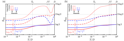
((a))

((b))

FIG. S3: Impurity entropy per impurity for two and three channels (red and blue, respectively) and up to three impurities, with $2J=\Gamma=D/8$, and different choices of NRG parameters: (a) $\Lambda=3,N_{K}\leq 12000$ converges to the correct low-energy fixed point, but displays truncation artifacts at high temperatures. (b) Parameters as in Fig. 2 in the main text: $\Lambda=6$ ($\Lambda=8$) for 1,2 (3) impurities, and $N_{K}\leq 12000$, which eliminate the artifacts.

If we take $D\gg J,\Gamma$, then in the first few NRG iterations the Wilson chain couplings are larger than the bare effective-impurity energy scales $J$ and $\Gamma$, and we cannot discriminate between different impurity many-body states. Thus, the we need to keep many states, i.e., we have a large $N_{E\left(n\right)}$, but due to the colossal size of the effective impurity, for reasonable $\Lambda=3$ we quickly saturate the $N_{K}$ limit and are forced to discard some required states. As a result we lose accuracy, which leads to an artificial drop in the impurity entropy at high temperatures in Fig. S3(a). Once we go below the bare energy scales, we start seeing the separation between the impurity states, and those of higher energy no longer mix with those of lower energy, so that they can be discarded. Thus, in this regime the number of kept multiplets $N_{E\left(n\right)}$ required for the same accuracy is smaller, and falls beneath the threshold $N_{K}$. Going below $T_{K}$, the required $N_{E\left(n\right)}$ shrinks even further. The errors accumulated from the uncontrolled truncations at the beginning of the chain enter the RG Hamiltonian in the form of irrelevant corrections, and so once we can keep enough multiplets, the RG flow corrects itself. As a result the impurity entropy, which is explicitly extracted from the RG Hamiltonian, also corrects itself, and follows the universal curve of the single-impurity entropy, multiplied by the number of impurities. We can improve the situation at high energies without compromising the low-energy behavior by relying on the observation that the impurity entropy is not very sensitive to $\Lambda$. Thus, taking relatively large $\Lambda=6,8$ we are able to reduce the number of required kept multiplets to what is tractable even above the bare scales, hence eliminate the artifacts while maintaining an overall correct behavior, as demonstrated in Fig. S3(b).

IV.2 $F$ Matrices

Turning to the eigenfunctions, they are more sensitive than the spectrum, and hence may suffer uncorrectable errors in the early regime. This affects observables which depend on them, such as the interimpurity spin correlators $\mathbf{S}_{m}\!\cdot\mathbf{S}_{m^{\prime}}$ and the extracted $F$ matrices. We thus wish to mitigate these errors by taking the shortest route to the low-energy anyonic fixed point. This is achieved by taking $J\gtrsim\Gamma$ so that $T_{K}$ is also of the same order. We take all three to be smaller than the artificial cutoff $D$, so that it does not lead to significant errors, but not much smaller so that we have a small region in which we have to carry out uncontrolled truncations. In what follows we will quantitatively demonstrate this.

For three impurities, we defined (in the main text) the $2\times 2$ matrices $\mathbf{s}_{mm^{\prime}}$ as the projection of the spin correlators $\mathbf{S}_{m}\!\cdot\mathbf{S}_{m^{\prime}}=\mathbb{1}_{\mathrm{2CK}}\otimes\mathbf{s}_{mm^{\prime}}$ onto the fusion space. We then found that they had one negative (singletlike) and one positive (tripletlike) eigenvalue, with eigenstates denoted by $\Ket{0_{mm^{\prime}}}$ and $\Ket{1_{mm^{\prime}}}$, respectively. We now define $\alpha_{mm^{\prime}}$ as (minus) the ratio between the two eigenvalues

$$\alpha_{mm^{\prime}}\equiv-\frac{s_{mm^{\prime}}^{-}}{s_{mm^{\prime}}^{+}}\quad;\quad\begin{cases}\mathbf{s}_{mm^{\prime}}\Ket{0_{mm^{\prime}}}=s_{mm^{\prime}}^{-}\Ket{0_{mm^{\prime}}}\\ \mathbf{s}_{mm^{\prime}}\Ket{1_{mm^{\prime}}}=s_{mm^{\prime}}^{+}\Ket{1_{mm^{\prime}}}\end{cases}.$$ (S12)

For two impurities we do not have the $\mathbf{s}_{mm^{\prime}}$ matrices, but can still define $\alpha_{12}$ as the ratio between the positive and negative eigenvalues of $\mathbf{S}_{1}\!\cdot\mathbf{S}_{2}$. In Fig. S4(b) we plot $\alpha_{mm^{\prime}}$ as a function of the ratio $J/\Gamma$, for both two (blue) and three (red) impurities and two channels. We observe that for $J\gtrsim\Gamma$ the ratio is minimal. If the two impurities are uncorrelated, i.e., $\left\langle\mathbf{S}_{m}\!\cdot\mathbf{S}_{m^{\prime}}\right\rangle_{T\to 0}=0$, then for two channels the two eigenvalues of the low-energy projected $\mathbf{S}_{m}\!\cdot\mathbf{S}_{m^{\prime}}$ should indeed be equal (and opposite in sign), i.e., $\alpha_{mm^{\prime}}=1$, as obtained analytically in Ref. [44]. However, even in the chiral case we have trivial correlations in the bath, which in the strong-coupling regime are then mirrored by interimpurity correlations. As these correlations should decay as the bath spin-density correlations, i.e., quadratically in the interimpurity distance, in Ref. [44], which assumes large separation, they were neglected with respect to the fusion-dependent contribution, which only decays as the first power of the distance. However, in the limit of short distances, as in our case, they survive and $\alpha_{mm^{\prime}}>1$. Still, we understand the regions of minimal $\alpha_{mm^{\prime}}$ as the best converged regions.

We also define a generalized $F$ matrix

$$F_{mm^{\prime\prime}}=\begin{pmatrix}\Braket{0_{mm^{\prime}}}{0_{m^{\prime}m^{\prime\prime}}}&\Braket{0_{mm^{\prime}}}{1_{m^{\prime}m^{\prime\prime}}}\\ \Braket{1_{mm^{\prime}}}{0_{m^{\prime}m^{\prime\prime}}}&\Braket{1_{mm^{\prime}}}{1_{m^{\prime}m^{\prime\prime}}}\end{pmatrix}\quad;\quad m\neq m^{\prime}\neq m^{\prime\prime},$$ (S13)

which describes the basis transformation from the definite fusion outcomes eigenstates of anyons $m,m^{\prime}$ to those of anyons $m^{\prime},m^{\prime\prime}$. Thus, $F_{13}$ corresponds to the standard $F$ matrix defined in Eq. (8) of the main text. $F_{23}$ can be obtained by braiding anyons 1 and 2, transforming according to $F_{13}$, and then unbraiding. $F_{12}$ can be obtained by a similar procedure, but it is actually already fully specified by $F_{12}=F_{23}^{\dagger}F_{13}$. In Table SII we present the extracted $F$ matrices for different choices of $J/\Gamma$, as well as the expected value for $\mathrm{SU}\!\left(2\right)_{2}$ anyons. We observe that also in this case we converge for $J\gtrsim\Gamma$, with the nearest-neighbor related term $F_{13}$ converging at a faster rate (already for $J=\Gamma$) than $F_{23}$.

((a))

((b))

FIG. S4: (a) Convergence of the critical chiral hopping amplitudes $t_{mm}^{\prime}$ to $\Gamma$ in the limit $\Gamma\ll D$ for different choices of $J/\Gamma$ (colors) and two (solid line) and three (circles, crosses) impurities. (b) Ratio between the magnitude of the negative and positive eigenvalues of the low-energy projected interimpurity spin correlators $\mathbf{S}_{m}\!\cdot\mathbf{S}_{m^{\prime}}$ as a function of $J/\Gamma$ with $\Gamma=D/8$. The solid line is obtained from two-impurity calculations while the circles and crosses are obtained from three-impurity calculations.

	$\begin{array}[]{c}\vspace{-1em}\hfil\\ F_{13}\\ \vspace{-1em}\hfil\end{array}$	$F_{23}$
$\begin{array}[]{c}\vspace{-1em}\hfil\\ J=\Gamma/2\\ \vspace{-1em}\hfil\end{array}$	$\frac{1}{\sqrt{2}}\!\!\left(\!\begin{smallmatrix}0.945&1.052\\ 1.052&-0.945\end{smallmatrix}\!\right)$	$\frac{1}{\sqrt{2}}\!\!\left(\!\begin{smallmatrix}0.60&\!\!\!+1.28ie^{\!+1.2i}\\ -1.28ie^{\!-1.2i}&\!\!\!-0.60\end{smallmatrix}\!\right)$
$\begin{array}[]{c}\vspace{-1em}\hfil\\ J=\Gamma\\ \vspace{-1em}\hfil\end{array}$	$\frac{1}{\sqrt{2}}\!\!\left(\!\begin{smallmatrix}0.992&1.008\\ 1.008&-0.992\end{smallmatrix}\!\right)$	$\frac{1}{\sqrt{2}}\!\!\left(\!\begin{smallmatrix}0.83&\!\!\!+1.15ie^{\!+0.3i}\\ -1.15ie^{\!-0.3i}&\!\!\!-0.83\end{smallmatrix}\!\right)$
$\begin{array}[]{c}\vspace{-1em}\hfil\\ J=2\Gamma\\ \vspace{-1em}\hfil\end{array}$	$\frac{1}{\sqrt{2}}\!\!\left(\!\begin{smallmatrix}1.003&0.997\\ 0.997&-1.003\end{smallmatrix}\!\right)$	$\frac{1}{\sqrt{2}}\!\!\left(\!\begin{smallmatrix}1.05&\!\!\!+0.95ie^{\!-0.1i}\\ -0.95ie^{\!+0.1i}&\!\!\!-1.051\end{smallmatrix}\!\right)$
$\begin{array}[]{c}\vspace{-1em}\hfil\\ \text{Expected}\\ \vspace{-1em}\hfil\end{array}$	$\frac{1}{\sqrt{2}}\!\!\left(\begin{smallmatrix}1&1\\ 1&-1\end{smallmatrix}\right)$	$\frac{1}{\sqrt{2}}\!\!\left(\begin{smallmatrix}1&+i\\ -i&-1\end{smallmatrix}\right)$

TABLE. SII: Numerically extracted $F$ matrices for different choices of $J/\Gamma$ with $\Gamma=D/8$. The last row displays the expected $F$ matrices of $\mathrm{SU}\!\left(2\right)_{2}$ anyons.

IV.3 Spectrum

In Sec. II we analyze the low-energy fixed point spectrum, which we can compare with the finite-size spectrum obtained from the CFT ansatz. The two should agree for $\Lambda\to 1$ which takes NRG back to the continuum limit, while larger $\Lambda$ induces “corrections” to the NRG spectrum. For $\Lambda=3$ these corrections become significant, i.e., lead to artificial splitting which is larger than the level spacing, already at low energy levels, so that the comparison with the CFT spectrum becomes difficult. Note that these deviations to not affect “global” spectrum properties such as the impurity entropy. Thus, only for the spectrum presented in Fig. S1, we we take smaller $\Lambda=2$. However, this renders the regime between $D$ and $J,\Gamma$ inaccessible within our computational resources. In order to overcome this challenge, we employ a useful NRG trick of taking the physical parameters $J$ and $\Gamma$ to be larger than the sharp cutoff $D$. This guarantees that already at the first NRG iteration we can discard the high-energy states of the effective-impurity, as the Wilson-chain couplings, which are smaller than $D$, cannot mix them with the low-energy states. We thus completely skip the difficult regime, and allow the RG flow to correct errors introduced by this artificial choice of parameters. Tuning the chiral hopping amplitudes $t_{mm}^{\prime}$ in this case, we find that they deviate significantly from $\Gamma$ and are as small as $0.4\Gamma$, as shown in Fig. S4(a). This is understandable, as their expected value of $\Gamma$ was only derived in the limit of $D\to\infty$, which is clearly not the case here.

IV.4 Fine-Tuning to Chirality

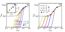
((a))

((b))

FIG. S5: Impurity entropy as a function of temperature for two impurities and two channels, when deviating from the chiral critical point (gray). All quantities are taken in units of $\Gamma$, with the Kondo coupling $J=\Gamma/2$, and $\Lambda=6$. (a) Deviations from chirality when fixing $t^{\prime}=\Gamma$ and varying the sharp cutoff $D$. Large $D/\Gamma$ requires $N_{K}\leq 8000$ kept multiplets in order to negate truncation effects which shift $t_{c}^{\prime}$. The low-energy chirality breaking scale $T^{*}$ (circles) is shown to be linear in $\Gamma/D$ (inset). (b) Deviations from chirality for $D=8\Gamma$ with positive (solid) and negative (dashed) deviations of $t^{\prime}-t_{c}^{\prime}$. Here $N_{K}\leq 2500$ suffices.

We now return to study the chirality-breaking effects of the sharp numerical cutoff $D$, and their remedy by numerically fine-tuning the imaginary hopping amplitudes $t_{mm^{\prime}}^{\prime}$. We focus on the two-impurity case, so that we have only a single hopping amplitude $t^{\prime}\equiv t_{12}^{\prime}$, and on two channels, so that we can significantly crank up the different numerical parameters within reasonable resources, but the following discussion is equally valid for more impurities and channels. In the absence of the sharp cutoff, $t^{\prime}$ is equal to the value of the soft cutoff $\Gamma$, rendering the system chiral. Fixing $t^{\prime}=\Gamma$ and $J$ (and thus $T_{K}$) with respect to $\Gamma$, in Fig. S5(a) we plot the impurity entropy for different ratios $D/\Gamma>1$ (approaching $D\to\infty$). Observe that it follows the universal curve of two infinitely separated impurities down to some low-energy scale $T^{*}$ which violates chirality. Defining $T^{*}$ by a deviation of 1% from the universal curve (circles), we find that it decays linearly in the ratio between the soft and sharp cutoffs $\Gamma/D$ (inset). Thus, in the presence of a sharp cutoff and when fixing $t^{\prime}=\Gamma$, the effective system is chiral only in an intermediate regime between the two energy scales $T^{*}$ and $D$.

This behavior mimics the effect of the bulk bands (Landau levels), which we have mostly ignored in this work, choosing to focus on the chiral edge mode residing in the band gap. The bulk band gap sets a finite bandwidth for the chiral mode, akin to $D$, while virtual process through the bulk bands mediate effective RKKY interactions at a low-energy scale $K$, which violates chirality, akin to $T^{*}$. However, whereas $T^{*}$ decays linearly with the artificial ratio between the two cutoffs $\Gamma/D$, the physical $K$ decays exponentially with both the bulk gap and the interimpurity distance [40, 41, 42]. This difference is not surprising, as in the effective model we have first taken the limit of an infinite band gap (so that $K\to 0$), then a small interimpurity separation (but still larger than the gap-induced short-distance scale), and only then reintroduced the artificial cutoff $D$ out of numerical necessity. Due to the exponential decay of the physical low-energy scale $K$, it is reasonable to assume that in an experiment it is negligible, and to thus also eliminate it (and its equivalent $T^{*}$) in the numerical analysis by tuning $t^{\prime}$ to be equal to $t_{c}^{\prime}$, as we now further elaborate.

In the absence of the cutoff $D$, the dictated $t_{c}^{\prime}=\Gamma$ sits at the critical point of a quantum phase transition of the effective model, with $T^{*}=0$, so that the system remains chiral down to arbitrarily small energy scales. The introduction of the sharp cutoff might shift the critical value $t_{c}^{\prime}$ away from $\Gamma$, but is not expected to affect the chiral nature of quantum critical point, as indeed observed numerically. Thus, for a given set of numerical parameters, and foremost $D$, we can numerically search for $t_{c}^{\prime}$ (there are many valid observables for the search, e.g., $\left\langle\mathbf{S}_{1}\!\cdot\mathbf{S}_{2}\right\rangle_{T\to 0}$, $S_{\mathrm{imp}}^{T\to 0}$, and in practice we look at the ground-state degeneracy of the effective NRG Hamiltonian at some late iteration). Note that this procedure accounts also for other chirality breaking effects, such as the NRG discretization and truncation, which also shift $t_{c}^{\prime}$, although to a lesser extent than the sharp cutoff (this becomes apparent when the cutoff is very large, so that its effect is small). Having found $t_{c}^{\prime}$, we can study deviations from it, as shown in Fig. S5(b), both for $t^{\prime}>t_{c}^{\prime}$ (solid) and $t^{\prime}<t_{c}^{\prime}$ (dashed). Observe that the energy scale of the deviation from the universal curve ($t^{\prime}=t_{c}^{\prime}$ or two infinitely separated impurities) is simply $\left|t^{\prime}-t_{c}^{\prime}\right|$ (full circles).

We thus understand that if we fix $t^{\prime}=\Gamma$, as in Fig. S5(a), then the low-energy chirality breaking scale is $T^{*}=\Gamma-t_{c}^{\prime}$, and is consistent with the linear scaling of $1-t_{c}^{\prime}/\Gamma$ in Fig. S4(a). But we also understand that setting $t^{\prime}=t_{c}^{\prime}$ eliminates the low-energy chirality breaking scale, even in the presence of a finite bandwidth. As the physical low-energy chirality breaking term decays exponentially, we find this choice better represents an experimental setup.