The intrinsic reddening of the Magellanic Clouds as traced by background galaxies – III. The Large Magellanic Cloud

Abstract

We present a map of the total intrinsic reddening across $\simeq$ 90 deg² of the Large Magellanic Cloud (LMC) derived using optical ($ugriz$) and near-infrared (IR; $YJK_{\rm{s}}$) spectral energy distributions (SEDs) of background galaxies. The reddening map is created from a sample of 222,752 early-type galaxies based on the lephare $\chi^{2}$ minimisation SED-fitting routine. We find excellent agreement between the regions of enhanced intrinsic reddening across the central ($4\times 4$ deg²) region of the LMC and the morphology of the low-level pervasive dust emission as traced by far-IR emission. In addition, we are able to distinguish smaller, isolated enhancements that are coincident with known star-forming regions and the clustering of young stars observed in morphology maps. The level of reddening associated with the molecular ridge south of 30 Doradus is, however, smaller than in the literature reddening maps. The reduced number of galaxies detected in this region, due to high extinction and crowding, may bias our results towards lower reddening values. Our map is consistent with maps derived from red clump stars and from the analysis of the star formation history across the LMC. This study represents one of the first large-scale categorisations of extragalactic sources behind the LMC and as such we provide the lephare outputs for our full sample of $\sim$ 2.5 million sources.

1 Introduction

The Magellanic Clouds contain stellar populations spanning all ages which thanks to their proximity ($\sim 50-60$ kpc) have allowed a number of investigations. The study of star formation at lower ($0.2-0.5$ Z_⊙) metallicities (e.g. Gouliermis, Hony & Klessen, 2014; Zivkov et al., 2018), the extragalactic distance scale (and by extension the Hubble constant $H_{0}$, e.g. de Grijs, Wicker & Bono, 2014; de Grijs & Bono, 2015; Riess et al., 2019; Freedman et al., 2020), and the metallicity dependence of the period–luminosity relation of variable stars (see e.g. Gieren et al., 2018; Groenewegen, 2018; Muraveva et al., 2018; Ripepi et al., 2019) are examples of investigations dependent upon an understanding of the amount and spatial distribution of dust across the galaxies. These studies use stellar populations of different ages to quantify the reddening in the Magellanic Clouds which results in statistically significant differences (this is further complicated by variations in metallicity, three-dimensional distributions of the stars and dust, etc.). On average, reddening maps based on young stellar populations such as Classical Cepheids or young open clusters produce maps emphasising the high levels of reddening typical of those areas of ongoing or recent star formation (Nayak et al., 2018; Joshi & Panchal, 2019); on the contrary, maps based on older stellar populations such as red clump and RR Lyrae stars systematically result in lower levels of reddening (see e.g. Zaritsky et al., 2002; Muraveva et al., 2018; Górski et al., 2020; Cusano et al., 2021).

The differences in colour excess, $\Delta E(B-V)$, can have a large influence on the inferred value for the Hubble constant and on the three-dimensional structure derived from stars (e.g. Ripepi et al., 2017; Choi et al., 2018). For example, an $\Delta E(B-V)=0.06$ mag difference between Haschke, Grebel & Duffau (2011) and Górski et al. (2020) studies, both using data from the third phase of the Optical Gravitational Lensing Experiment (OGLE-III; Udalski, 2003), implies a difference in the value of the Hubble constant larger then 3 km s^-1 Mpc^-1 (see e.g. section 3.1 of Riess et al., 2009). The presence of dust influences the location of stars in colour–magnitude diagram (CMD) which is often used to select different stellar types to study their spatial distribution (e.g. El Youssoufi et al., 2019) and kinematics (e.g. Niederhofer et al., submitted). An independent map of the internal reddening of the Magellanic Clouds would also reduce the residuals between data and models in regions of the CMD which are used simultaneously to infer the reddening, distance modulus and star formation history (SFH) of the galaxies (e.g. Rubele et al., 2018; Mazzi et al., 2021). Small-scale reddening variations present in maps obtained from individual stars (e.g. Tatton et al., 2021) and in specific regions of the galaxies (e.g. De Marchi, Panagia & Milone, 2021) may not be easy to reconcile with large-scale studies based on broadly distributed tracers.

In Bell et al. (2019, hereafter Paper I) we piloted a method to map the intrinsic reddening of a foreground extinguishing medium using the spectral energy distributions (SEDs) of background galaxies. This approach takes away the dependency on reddening values of stellar populations and allows us to study the total reddening by sampling the full column depth of the extinguishing medium. In Bell et al. (2020, hereafter Paper II) we applied this method to a $\simeq$ 34 deg² region of the Small Magellanic Cloud (SMC) covered by both the Survey of the MAgellanic Stellar History (SMASH; Nidever et al., 2017) and the Visible and Infrared Survey Telescope for Astronomy (VISTA) survey of the Magellanic Clouds system (VMC; Cioni et al., 2011). In Paper II, adopting galaxies with low intrinsic reddening, we found signs of higher intrinsic reddening in the main body of the galaxy compared with its outskirts. Our maps agree with those in the literature which were created using young stars whereas there are some discrepancies with maps derived from longer-wavelength far-IR emission and from old stars. These discrepancies may be due to biases in the sample or uncertainties in the far-IR emissivity of the optical properties of the dust grains. In this study, we map the total intrinsic reddening across a $\simeq$ 90 deg² region of the Large Magellanic Cloud (LMC) combining observations from the SMASH and VMC surveys.

The structure of this paper is as follows. In Section 2 we describe the processes involved in creating and fitting the SEDs of background galaxies as well as provide a comparison of the results of the SED fitting with other extragalactic studies. The details of how we create our intrinsic reddening map of the LMC are presented in Section 3. We discuss our reddening map and compare it with literature reddening maps of the LMC based on different tracers in Section 4, and summarise our findings in Section 5.

2 Creating and fitting SEDs of galaxies

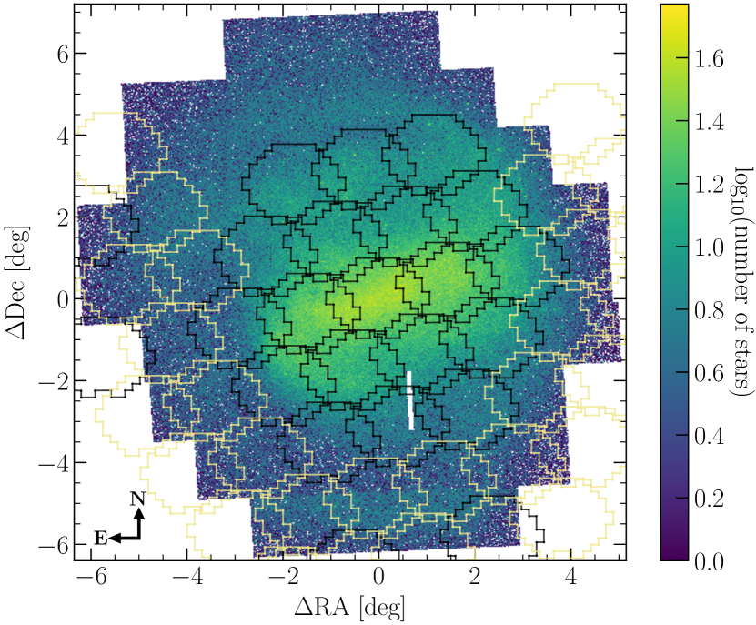
Figure 1: Stellar density distribution of the LMC from the VMC survey. The colour bar refers to the number of stars per bin, where the bin size is of $0.4\times 0.4$ arcmin². The origin of the plot corresponds to the centre of the LMC as given by the HYPERLEDA catalogue of Paturel et al. (2003). The hexagons denote the positions of the SMASH fields that overlap with the VMC coverage of the LMC. Black fields denote those for which $ugriz$ data are available, whereas khaki fields represent those for which only $griz$ data are available. The combined SMASH–VMC footprint is $\simeq$ 90 deg². A gap at $\Delta$RA $\simeq 0.7$ deg is currently being observed.

Our data set consists of optical $ugriz$ and near-IR $YJK_{\rm{s}}$ photometry taken as part of the SMASH and VMC surveys, respectively, that cover the wavelength range 0.3–2.5 $\mu$m. The combined SMASH–VMC footprint of the LMC is shown in Fig. 1 and covers an area of $\simeq$ 90 deg². We note two significant differences regarding the SMASH data used in this study compared to that used in Papers I and II. First, as shown by the different colour DECam fields in Fig. 1, only the central regions of the LMC (black hexagons) are fully covered by deep $ugriz$ data. The surrounding fields (khaki hexagons) represent fields for which only $griz$ data are available. Second, whereas the fields with full 5-band data consist of deep exposures (999 s in $uiz$ and 801 s in $gr$), in addition to three sets of short 60 s exposures in $ugriz$ with large half-CCD offsets between each set (to cover the gaps between the CCDs), fields with 4-band data consist only of two sets of short 60 s exposures in $griz$ (again with half-CCD offsets to cover the gaps between CCDs; see section 3 of Nidever et al., 2017 for details).

For the study of the LMC we have made three notable changes, relative to the methodology applied to the SMC and laid out in Papers I and II; namely the selection of background galaxies, the treatment of foreground Milky Way (MW) reddening and the use of ancillary radio data to separate the Active Galactic Nuclei (AGN) population prior to fitting the SEDs. We refer the reader to Paper I of this series for a discussion of each step of the process, including the choice of galaxy templates, redshift priors, extinction law, and photometric uncertainties.

2.1 Selection of background galaxies

Figure 2: a: Near-IR $J-K_{\rm{s}},K_{\rm{s}}$ CMD of tile LMC 3_4. The blue points denote objects selected as likely galaxies adopting the criteria of Papers I and II (see text), whereas the orange points represent those that are subsequently classified by lephare as ETGs. The error bars on the left denote the median photometric errors as a function of $K_{\mathrm{s}}$-band magnitude at 1 mag intervals b: As a, but the green points correspond to those for which the $K_{\rm{s}}$-band sharpness index is greater than 0.5. c: Same as b, however the pink points denote those of the green points lephare classifies as galaxies and the brown points represent the subset of these classified as ETGs. d: Histograms of the numbers of galaxies and ETGs as a function of $J-K_{\rm{s}}$ colour. The dashed line at a colour of $J-K_{\rm{s}}=0.8$ mag separates those that appear to be primarily blended stellar sources (at bluer colours) and those that are predominantly non-blended, extended sources (at redder colours).

The process of creating the galaxy SEDs has been extensively covered in Papers I and II. However, in light of our SMC analysis we have made some minor modifications that we describe below. In Paper II we noted that the number of early-type galaxies (ETGs) in the central regions of the SMC was limited due to incompleteness arising from the enhanced levels of crowding compared to the less-dense outer regions. The central regions of the LMC are even more affected by crowding and thus we have revised our selection in an effort to increase the number of ETGs in our sample.

Before explaining our updated selection criteria, it should be noted that our definition of an ETG is directly linked to the adopted templates in lephare. The galaxy templates we adopt are the so-called AVEROI_NEW templates and we classify an object as an ETG if lephare finds a lower minimum $\chi^{2}$ associated with the best-fitting galaxy template (compared to the best-fitting stellar template) and if the best-fitting galaxy template corresponds to a spectral type of Ell or Sbc (see section 3.1 of Paper I for details regarding the AVEROI_NEW templates).

Our selection of background galaxies is based on the VMC point-spread function (PSF) photometric catalogues (see Mazzi et al., 2021 for details). Panel a of Fig. 2 shows the CMD selection previously adopted in Papers I and II, namely retaining those that satisfy the following: $J-K_{\rm{s}}>1$ mag, $K_{\rm{s}}>15$ mag, an associated stellar probability of less than 0.33 and a $K_{\rm{s}}$-band sharpness index greater than 0.5. To increase our sample of ETGs we effectively need to include galaxies at bluer colours. If we simply remove the colour cut, however, the use of the stellar probability still severely limits the inclusion of bluer galaxies (see e.g. Fig. 2 of Paper I).

To assess how best to modify our galaxy selection, we first retain only those objects with a $K_{\rm{s}}$-band sharpness index greater than 0.5 (Fig. 2b). These objects are then processed through lambdar (see Section 2.2) and lephare (see Section 2.4) to determine which ones are classified as galaxies and, more specifically for our purposes, ETGs (the brown and purple points in Fig. 2c, respectively). There is clearly a bimodality in the distribution of galaxies and ETGs as a function of $J-K_{\rm{s}}$ colour. Dividing the ETG sample at a colour of $J-K_{\rm{s}}=0.8$ mag and visually inspecting $K_{\rm{s}}$-band image cut-outs we note that the vast majority of objects at bluer colours (of which there are 369 in tile LMC 3_4, a tile in the outer disc of the LMC) are stellar blends, whereas those at redder colours (of which there are 4430) appear to be predominantly non-blended extended sources. Retaining such a large number of stellar blends in our ETG sample would have a non-negligible effect when creating the reddening maps. Furthermore, it is not feasible to visually inspect all ($\sim$300,000) candidate ETGs across the combined SMASH–VMC coverage of the LMC. The $J-K_{\rm{s}}$ colour distribution of known QSOs, which is similar to that of galaxies, shows a clear edge at $0.8$ mag which is also away from stellar sources (Cioni et al., 2013). The final number of objects classified as ETGs in tile LMC 3_4 based on a revised colour selection criteria ($J-K_{\rm{s}}>0.8$ mag) is 4430, which when compared to the 3361 one would find using our previous selection criteria represents an increase in sample size of almost a third.

2.2 lambdar photometry

Fluxes for each of our targets are measured using the Lambda Adaptive Multi-Band Deblending Algorithm in R (lambdar, v0.20.7; Wright et al., 2016). This version has minor developments (with respect to v0.20.5 that was used in Paper II), that improve the stability and fidelity of the PSF estimation procedure. We use these new developments (and our knowledge that our fields are crowded with point sources) to specify conservative requirements on which sources are selected for use in the PSF estimation. Specifically, we opt for a maximum number of point sources to be used in the PSF estimation of 500 per-chip (a chip corresponds to a detector or a charge coupled device in the VISTA and SMASH images, respectively), with a minimal radial separation (from possible contaminating sources) of 10 pixels (or $\sim$ $3.4$ arcsec). The latter condition often produces many more than 500 sources per-chip (especially in very crowded regions), and in these cases the code iteratively increases the minimum radial separation until 500 sources are selected; that is, the code selects the 500 most isolated point sources for use in the PSF estimation.

Paper I provides a comprehensive discussion regarding the measurement of fluxes in addition to the calibration of both the optical and near-IR data sets onto an AB magnitude system. We adopt the fluxes measured using a default circular aperture of diameter 3 arcsec. The $Y$-, $J$- and $K_{\rm{s}}$-band deep stacks from which lambdar measures the fluxes were downloaded from the VISTA Science Archive (VSA; Cross et al., 2012) and have been processed by the Cambridge Astronomy Survey Unit (CASU). Unlike the deep stacks used in Papers I and II that were created using the VISTA Data Flow System (VDFS; Irwin et al., 2004) v1.3, the deep stacks used in this study have been processed using v1.5 (González-Fernández et al., 2018; see also the CASU webpage). The main difference between the two versions is in the determination of the zero-points and as such we apply the offsets listed in eqs. C7–C11 of González-Fernández et al. (2018) in addition to those noted in section 2.4 of Paper I. The zero-point differences between the two versions amount to $0.01-0.02$ mag which will have a minimal influence on our study (cf. Fig. 2). Other differences refer to tiles, the combined product of deep stacks, which we do not use. The $u$-, $g$-, $r$-, $i$- and $z$-band data were treated in exactly the same way as described in Paper I.

2.3 Accounting for foreground Milky Way reddening

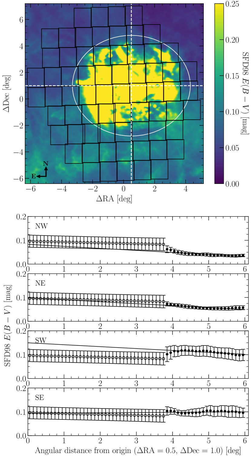
Figure 3: Top panel: Schlegel et al. (1998) foreground MW and residual intrinsic LMC reddening map. The black polygons represent the positions of the VMC tiles covering the LMC. The dashed white lines separate the LMC into different quadrants. The white circle (centred at $\Delta\mathrm{RA}=0.5$, $\Delta\mathrm{Dec}=1.0$ deg and with a radius of 3.8 deg) marks the region within which the SFD98 $E(B-V)$ values are unreliable. Bottom panel: SFD98 $E(B-V)$ values in each quadrant as a function of angular distance. The solid points denote the median $E(B-V)$ value calculated from the SFD98 reddening map between distances of 3.8 and 6 deg in steps of 0.1 deg and the associated error bars represent the standard deviation in that annulus. The linear best fit to the solid points in each quadrant is also shown as the straight black line. The open points are the same in each panel and denote the median of the four fits in steps of 0.1 deg covering the region within which the SFD98 $E(B-V)$ values are unreliable. The error bars signify the standard deviation between the four fits.

To produce a dust map of the LMC we need to take into account the reddening along the line-of sight. In Papers I and II we adopted a rather rudimentary method to account for the foreground MW reddening towards the SMC by adopting a mean $E(B-V)$ value for all objects based on the Schlegel, Finkbeiner & Davis (1998, hereafter referred to as SFD98) reddening map purposefully neglecting the main body and Wing of the SMC (see fig. 4 of Paper I). Whilst such a treatment, to zeroth order, should adequately reflect the “average” foreground MW reddening, it is likely to hide fluctuations or trends in $E(B-V)$ across the SMC. In light of this, we hereby adopt a revised method that we describe below.

The top panel of Fig. 3 shows the SFD98 foreground MW and residual intrinsic LMC reddening map with the positions of the VMC tiles covering the LMC overlaid. The inner circle (centred at $\Delta\mathrm{RA}=0.5$, $\Delta\mathrm{Dec}=1.0$ deg and with a radius of 3.8 deg) marks the region within which the SFD98 $E(B-V)$ values are unreliable due to insufficiently resolved temperature structures. Outside of this inner circle the SFD98 $E(B-V)$ values are believed to be reliable (see e.g. Schlegel et al., 1998; Skowron et al., 2021) and clearly show a significant amount of substructure in the high-latitude MW cirrus (this difference is especially noticeable in regions to the south and to the north of the LMC). For objects farther than 3.8 deg from the centre of the inner circle we simply de-redden the fluxes provided by lambdar using sfdmap. For objects within the inner circle, however, we construct a radial $E(B-V)$ profile from linear extrapolations of fits to regions outside of the inner circle.

The bottom panel of Fig. 3 shows the SFD98 $E(B-V)$ values as a function of angular distance from $\Delta\mathrm{RA}=0.5$, $\Delta\mathrm{Dec}=1.0$ deg. The solid points denote the median $E(B-V)$ value calculated in each quadrant between the two white circles in steps of 0.1 deg using sfdmap and the associated error bars represent the standard deviation in that annulus. The best-fitting linear curve to the solid points in each quadrant is also shown as the straight black line. The open points are the same in each panel and denote the median of the four fits in steps of 0.1 deg covering the region within which the SFD98 $E(B-V)$ values are unreliable. The error bars signify the standard deviation among the four fits. These open points represent the radial $E(B-V)$ profile that we adopt to de-redden the fluxes for objects that lie within the inner circle i.e. objects within this region are de-reddened according to their angular distance from $\Delta\mathrm{RA}=0.5$, $\Delta\mathrm{Dec}=1.0$ deg. From Fig. 3 it is clear that there are enhanced levels of reddening in the south-west quadrant with respect to the other three quadrants, and this likely accounts for the observed offset between the extrapolated line and the calculated radial profile within 3.8 deg in this quadrant which is not observed in the other quadrants. At the time of submission of our work to the journal, Chen et al. (2022) presented a dust map of the MW derived from the SED of stellar sources within 5 kpc. They combined astrometry from Gaia with optical and near-IR photometry from various large-scale surveys towards the Magellanic Clouds. Their MW reddening map towards the LMC shows an average $E(B-V)$ of 0.06 mag with values as high as 0.15 in the south of the disc (an area outside our inner circle). The small inhomogeneities and clumps in the inner regions do not appear to exceed this value (their Fig. 10). Our extrapolation corresponds to an average $E(B-V)$ of about 0.1 mag (Fig. 3) which is in line with the maximum values derived by Chen et al. (2022), but may overestimates by a few percent the extinction towards some specific lines of sights.

The extinction coefficients adopted to convert a given $E(B-V)$ value into an extinction in a specific bandpass are those listed in eq. 1 of Paper I and should be used in conjunction with the unscaled SFD98 $E(B-V)$ values as they already take into account the Schlafly & Finkbeiner (2011) recalibration. After de-reddening the fluxes and retaining only objects for which lambdar measures positive fluxes in at least four out of the eight available bandpasses, our full LMC sample contains 2,474,235 objects.

2.4 Fitting the SEDs with lephare

Papers I and II provide a comprehensive overview of fitting SEDs using lephare. However, we briefly discuss the notable difference in this work with respect to the earlier works in this series. In Papers I and II we primarily included quasi-stellar object (QSO)/AGN templates (hereafter collectively referred to as AGN) as the level of AGN contamination in our sample was unclear. With no comprehensive catalogue of AGN behind the SMC [except for the areas covered by, e.g, the XMM–Newton survey (Haberl et al., 2012) as well as incomplete spectroscopic samples (e.g. Kozłowski, Kochanek & Udalski, 2011; Kozłowski et al., 2013)] we included such templates to not only account for the presence of AGN, but also to provide more flexibility with regards to fitting the SEDs. The inclusion of the AGN templates in lephare likely resulted in degeneracies in the best-fitting templates as the number of objects classified as AGN in the full SMC sample was markedly higher than those lephare classified as galaxies (see table 2 of Paper II). This, in addition to the previously adopted criteria for selecting background galaxies from the deep VMC PSF photometric catalogues (see Section 2.1), likely contributed to the low number of ETGs in the central regions of the SMC.

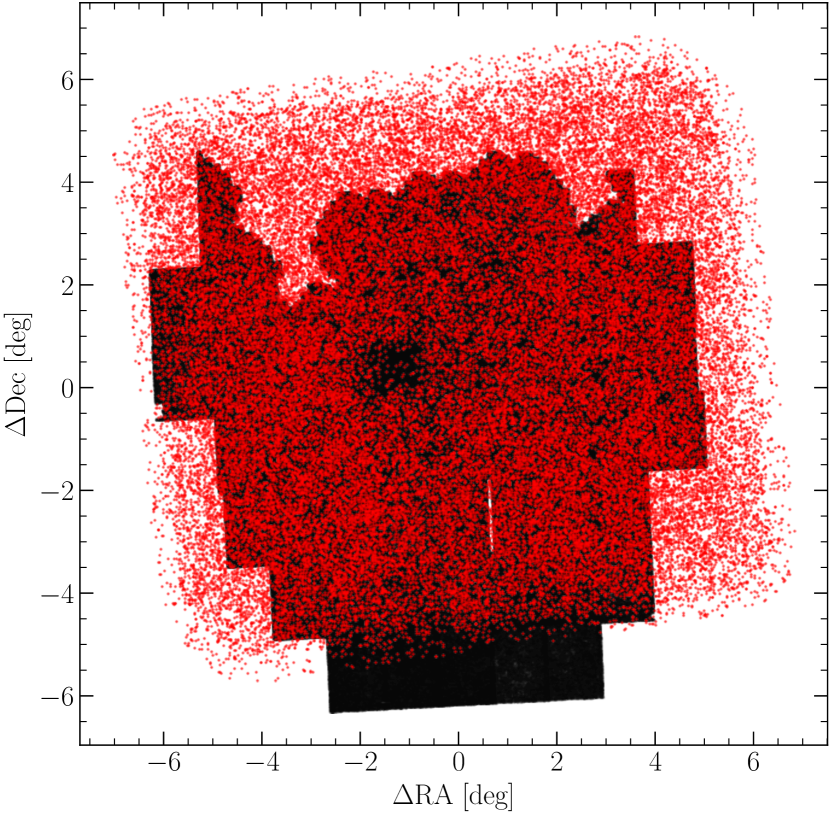
Figure 4: Positions of the 54,612 radio sources detected in the 888 MHz ASKAP EMU data towards the LMC (red points; Pennock et al., 2021) overlaid on the full SMASH-VMC sample (black points).

In this study we make use of the recently published catalogue of radio-detected sources in the direction of the LMC by Pennock et al. (2021) based on 888 MHz Australian Square Kilometre Array Pathfinder (ASKAP) Evolutionary Map of the Universe (EMU) radio continuum survey data. These data cover $\simeq$ 120 deg² and the catalogue contains 54,612 sources separated into Gold, Silver and Bronze categories (see section 3.2 of Pennock et al., 2021 for details). Although the catalogue also contains both MW sources in the foreground of the LMC as well as sources in the LMC itself, the vast majority of the radio sources are background objects, and in particular, AGN. Fig. 4 shows that the radio sources almost completely cover the full LMC sample, except for a significant fraction of the lowest row of VMC tiles (LMC 2_3–LMC 2_7). We can therefore use this catalogue to systematically and effectively remove AGN contaminants – as well as foreground interlopers – from our sample and ensure that we are not reliant upon lephare for such discrimination.

There are two primary reasons for separating the AGN from the full LMC sample. First, as demonstrated in Paper I, it is difficult to use AGN to create a reddening map due to the varying levels of intrinsic reddening. By removing AGN from the full LMC sample, they are unable to be misclassified by lephare and incorrectly incorporated into the creation of the reddening map. Second, the vast majority of spectroscopic redshifts for objects behind the LMC are associated with AGN. To test the validity of the lephare photometric redshifts it is therefore best to fit such objects with more representative AGN templates so as to minimise any potential biases introduced by using less well-suited galaxy templates. Following Pennock et al. (2021), we adopt a cross-match radius of 5 arcsec and find a total of 21,706 radio sources in the full LMC sample. Whilst the Pennock et al. (2021) catalogue is complete down to 0.5 mJy across the field and contains the majority of the spectroscopically confirmed AGN in the combined SMASH–VMC footprint of the LMC, we still identified an additional 122 AGN with spectroscopic redshift determinations from v7.2 of the Milliquas (Million Quasars) catalogue (Flesch, 2021) that were not present and include these to create our final AGN sample comprising 21,828 sources. These sources are subsequently removed from the full LMC sample, reducing its number to 2,474,235. Note that although the radio catalogue of sources in the direction of the LMC provided by Pennock et al. (2021) is the most sensitive to date, only $\sim$ 10–20 per cent of all AGN are radio-loud (see e.g. Ivezić et al., 2002; Jiang et al., 2007). We are therefore no doubt significantly underestimating the level of AGN contamination in our sample of extragalactic objects behind the LMC, although the EMU end-of-survey sensitivity should detect radio-quiet AGN out to $z\simeq 2$ (Norris et al., 2011).

We run lephare as described in Paper II on both the full LMC and AGN samples. We only use the empirical AVEROI_NEW galaxy templates for the LMC sample in addition to the stellar templates, whereas for the AGN sample we replace the galaxy templates with the 10 AGN templates described in Polletta et al. (2007, see section 3.1 of Paper I for details regarding these template libraries). As in Paper II, we allow additional intrinsic reddening [in terms of $E(B-V)$] to vary and allow this additional reddening for all galaxy/AGN types. Typically, additional reddening is only used for later-type galaxies (Sc and bluer/later; see e.g. Arnouts et al., 2007) and AGN (see e.g. Salvato et al., 2009) on the basis that the adopted templates may not fully account for the widely varying levels of dust observed in such galaxies/AGN. For ETGs, and particularly in the optical/near-IR regime we are interested in here, the range in dust is not as extreme and so the assumption is that the adopted templates fully account for their dust contents and thus additional reddening is not required. Our method of using ETGs as reddening probes essentially builds upon this assumption by suggesting that any additional reddening required by ETGs is due to a foreground extinguishing medium, in our case the LMC. Tables 1 and 2 provide the lephare outputs for the 2,474,235 and 21,828 sources in the full LMC and AGN samples, respectively. The associated $\chi^{2}$ values for the best-fitting templates imply that 61 per cent of the full LMC sample are galaxies (39 per cent stars) and 87 per cent of the AGN sample are AGN (13 per cent stars). Of the 61 per cent of objects classified as galaxies in the full LMC sample, 15 per cent (222,752) are classified as ETGs.

Table 1: A sample of the lephare output for the 2,474,235 sources in the full LMC sample. We only show the ID, RA and Dec. (J2000.0), the best-fitting photometric redshift with associated $1\sigma$ limits, the maximum likelihood photometric redshift with associated $1\sigma$ limits, the best-fitting galaxy template, the associated $\chi^{2}$ value for the best-fitting galaxy template and the best-fitting $E(B-V)$ value. The full table available as Supporting Information contains other parameters.

ID	RA (J2000.0)	Dec. (J2000.0)	$z_{\rm{BEST}}$	$z_{\rm{BEST}}^{-1\sigma}$	$z_{\rm{BEST}}^{+1\sigma}$	$z_{\rm{ML}}$	$z_{\rm{ML}}^{-1\sigma}$	$z_{\rm{ML}}^{+1\sigma}$	Template${}_{\rm{G}}^{a}$	$\chi^{2}_{\rm{G}}$	$E(B-V)$
	deg	deg									mag
1	73.77041	$-75.72749$	0.4906	0.4645	0.5143	0.4694	0.3974	0.5147	54	2.1045	0.05
2	73.82095	$-75.72746$	0.3292	0.3059	1.3738	1.1080	0.3329	1.5322	59	8.6474	0.00
3	73.78706	$-75.72451$	0.0200	0.0200	0.0277	0.0128	0.0041	0.0310	49	71.1816	0.15
4	73.74649	$-75.71641$	1.0280	0.7738	1.2179	0.9209	0.5290	1.1316	50	2.6083	0.15
5	73.50257	$-75.71626$	0.5961	0.5347	1.1331	0.9244	0.5870	1.2578	57	3.1876	0.50
6	73.83151	$-75.71592$	0.4862	0.4433	0.5389	0.4802	0.3976	0.5374	38	5.5756	0.00
7	73.48358	$-75.71535$	1.3214	1.3109	1.3322	1.3297	1.3041	1.3635	62	15.4637	0.40
8	73.77131	$-75.71414$	0.0555	0.0423	0.0667	0.0726	0.0423	2.8935	62	15.1095	0.05
9	73.76825	$-75.71168$	0.9478	0.7439	1.2849	0.9306	0.5771	1.1749	62	4.7682	0.30
10	73.82471	$-75.71136$	0.5050	0.4176	0.8201	0.5114	0.3058	0.7615	62	2.0733	0.10

^a Best-fitting galaxy templates are as follows: (1–21) E, (22–37) Sbc, (38–48) Scd, (49–58) Irr, (59–62) Starburst.

^b Context is a numerical representation in lephare specifying the combination of bands present in the input catalogue and is defined as $\sum_{i=1}^{i=N}2^{i-1}$, where $i$ is the band number (in our case $u=1$, $g=2$, …, $J=7$, and $K_{\rm{s}}=8$), and $N$ is the total number of bands.

Table 2: Same as Table 1, but for the 21,828 sources in the AGN sample.

ID	RA (J2000.0)	Dec. (J2000.0)	$z_{\rm{BEST}}$	$z_{\rm{BEST}}^{-1\sigma}$	$z_{\rm{BEST}}^{+1\sigma}$	$z_{\rm{ML}}$	$z_{\rm{ML}}^{-1\sigma}$	$z_{\rm{ML}}^{+1\sigma}$	Template${}_{\rm{Q}}^{a}$	$\chi^{2}_{\rm{Q}}$	$E(B-V)$
	deg	deg									mag
1	74.13216	$-74.39312$	1.1025	1.0778	1.1794	1.1353	1.0840	1.1957	6	10.2503	0.45
2	73.66724	$-74.35413$	0.7129	0.5553	0.9163	0.8019	0.6263	1.0059	4	3.3765	0.00
3	74.62965	$-74.33360$	1.0313	0.7321	1.4235	1.0588	0.6518	1.5054	5	7.6673	0.15
4	73.07838	$-74.29228$	0.3555	0.3540	0.3623	0.3559	0.3414	0.3722	10	121.5800	0.15
5	70.73015	$-74.10165$	1.0855	1.0737	1.2082	1.1423	1.0872	1.2030	6	10.8134	0.10
6	70.58080	$-74.08259$	1.0907	1.0138	1.1312	0.8248	0.6040	1.0886	3	8.9963	0.00
7	76.32935	$-74.59744$	1.0284	1.0141	1.0474	1.0428	1.0138	1.1032	3	33.3055	0.35
8	76.59007	$-74.57986$	1.2702	1.0548	1.2807	1.2378	1.0576	1.2750	10	9.9513	0.00
9	75.99906	$-74.47083$	1.0737	1.0768	1.0807	1.0792	1.0655	1.0933	6	15.1357	0.40
10	77.26805	$-74.42954$	0.3326	0.3187	0.3475	0.3332	0.3125	0.3541	1	52.6541	0.05

^a Best-fitting AGN templates are as follows: (1) Seyfert 1.8, (2) Seyfert 2, (3–5) type-1 QSO, (6–7) type-2 QSO, (8–9) Starburst/ULIRG, (10) Starburst/Seyfert 2.

^b Context is a numerical representation in lephare specifying the combination of bands present in the input catalogue and is defined as $\sum_{i=1}^{i=N}2^{i-1}$, where $i$ is the band number (in our case $u=1$, $g=2$, …, $J=7$, and $K_{\rm{s}}=8$), and $N$ is the total number of bands.

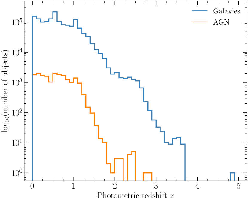
Figure 5: Distribution of redshifts for galaxies (blue) and AGN (orange) classified by lephare.

Fig. 5 shows the photometric redshift distributions for the 1,504,987 objects classified as galaxies and the 19,017 objects classified as AGN in the full LMC and AGN samples, respectively. As discussed in section 2.3 of Paper II, we choose the photometric redshift from the median of the maximum likelihood distribution ($z_{\rm{ML}}$) or if this is not available the one with the minimum $\chi^{2}$ value ($z_{\rm{BEST}}$). The median redshift of both samples is very similar ($z_{\rm{med}}=0.56$ and 0.57 for the galaxy and AGN samples, respectively). Although this median redshift is almost identical to that of the objects classified as galaxies behind the SMC in Paper II, we refrain from making a direct comparison between the two galaxy populations due to the combined effects of the different methods of selecting background galaxies as well as the use of different template sets between the two studies. Any conclusions drawn from such a comparison (e.g. the different distribution of spectral types) should be treated with caution and not used to argue for systematic differences between the two galaxy populations. Although such a comparison would be worthwhile, this would necessitate a complete redetermination and analysis of the SMC sample that is beyond the scope of this study.

2.4.1 Effects of missing $u$-band data

Figure 6: Distributions of galaxies redshifts in the full LMC sample. The blue line denotes galaxies for which the SED comprises all eight available bands (from $u$ to $K_{\rm{s}}$). The orange line represents the same sample of galaxies as shown by the blue line, however we have removed the measured $u$-band fluxes and re-run through lephare. The green line illustrates galaxies for which there are no $u$-band data available but have measured fluxes in the seven remaining bands (from $g$ to $K_{\rm{s}}$).

It is worth noting that we have not yet discussed the effects of non-complete $u$-band coverage across the combined SMASH–VMC footprint of the LMC. From Fig. 1 it is evident that only the central regions of the LMC have $u$-band data from SMASH, as well as a few isolated regions in the outskirts. In Fig. 6 we show the photometric redshift distributions for objects classified as galaxies in the full LMC sample. There are three samples of galaxies shown in Fig. 6: i) objects that have measured fluxes in all eight available bands (from $u$ to $K_{\rm{s}}$), ii) as i) but with the $u$-band fluxes removed and re-run through lephare and iii) objects for which no $u$-band data are available, but which have measured fluxes in the remaining seven bands (from $g$ to $K_{\rm{s}}$). The number of galaxies in each sample is limited to 350,000 to better illustrate systematic differences between the samples. The effect of simply removing the $u$-band data (where available) is small but noticeable, in the sense that there are some variations in the redshift distributions across the whole redshift range, but overall the distributions resulting from samples (i) and (ii) are broadly similar in terms of median redshift and shape (cf. $z_{\rm{med}}=0.36$ for the 8-band SED sample and $z_{\rm{med}}=0.44$ for the reprocessed sample after removing the $u$-band data). The resulting samples of ETGs are also similar. In contrast, the redshift distribution for objects for which no $u$-band data are available is markedly different, both in terms of median redshift ($z_{\rm{med}}=0.59$) and as regards the apparent dearth of galaxies at higher redshifts. These differences likely stem from the SMASH observing strategy for which only regions with full $ugriz$ coverage have deep exposures, whereas the regions with only $griz$ coverage are covered by short exposures (see Section 2 for details). The latter sample of ETGs will be similar to that of ETGs within the same magnitude ranges resulting from deeper observations. This further reinforces the importance of the $u$ band as a powerful diagnostic to discriminate between low ($z\lesssim 0.5$) and higher redshift galaxies (see e.g. Bellagamba et al., 2012; Bisigello et al., 2016) as well as the need for homogeneous coverage (in terms of photometric bandpasses and exposure time) across the survey area.

2.4.2 Comparison of spectroscopic and photometric redshifts for AGN behind the LMC

Figure 7: Histogram showing the differences between the spectroscopically determined redshifts of AGN behind the LMC and the corresponding photometric redshifts calculated by lephare. The various statistics regarding the comparison of the two redshift determinations are discussed in the text.

Table 3: Spectroscopically determined and photometric redshifts for AGN behind the LMC. The full table is available as Supporting Information.

Name	$z_{\mathrm{spec}}$	$z_{\mathrm{phot}}$	Ref.
PMN J0601–7238	0.001	$0.014^{+0.031}_{-0.009}$	1
6dF J050434.2–734927	0.045	$0.186^{+0.120}_{-0.121}$	2
MQS J053242.46–692612.2	0.059	$0.058^{+0.041}_{-0.050}$	3
MQS J043522.69–690352.9a	0.061	$0.096^{+0.004}_{+0.004}$	3
PGC 3095709	0.064	$0.158^{+0.068}_{-0.092}$	4
J050550.3–675017	0.070	$0.155^{+0.071}_{-0.052}$	5
1E 0534–6740a	0.072	$0.234^{+0.006}_{+0.006}$	6
PGC 88452	0.075	$0.086^{+0.024}_{-0.037}$	7
MQS J045554.57–691725.6	0.084	$0.005\pm 0.003$	3
MQS J043632.30–704238.1	0.142	$0.182^{+0.207}_{-0.116}$	3

Notes: ^aAssociated 1$\sigma$ limits on $z_{\mathrm{BEST}}$ are unphysical (see section 2.3 and footnote 4 of Paper II for details).

^bAssociated $\chi^{2}$ value for best-fitting stellar template is lower than $\chi^{2}$ value for best-fitting AGN template.

References: (1) Ajello et al. (2020), (2) Jones et al. (2009), (3) Kozłowski et al. (2013), (4) Cowley et al. (1984), (5) Dobrzycki et al. (2005), (6) Crampton et al. (1997), (7) Cristiani & Tarenghi (1984), (8) Kozłowski et al. (2012), (9) Wang et al. (1991), (10) Dobrzycki et al. (2002), (11) Tinney (1999), (12) Geha et al. (2003), (13) Ivanov et al. (2016), (14) Kostrzewa-Rutkowska et al. (2018).

As an additional test we compare the derived photometric redshifts to spectroscopic redshifts of 189 AGN. Table 3 lists the comparison between the values and Fig. 7 highlights a median difference of $\Delta z_{\rm{med}}=-0.009$, where $\Delta z_{\rm{med}}=z_{\rm{spec}}-z_{\rm{phot}}$, and median absolute deviation of $\Delta z_{\rm{MAD}}=0.191$. Note that of the 189 AGN in our sample, five (MQS J050010.83–700028.5, 1E 0547–6745, MQS J054400.43–705846.2, MQS J043200.60–693846.5 and MQS J052528.91–700448.6) are classified as stars by lephare. The statistics reported here, with the exception of the bias, outlier fraction (OLF), are very similar to those reported in Paper II for the sample of 46 AGN behind the SMC. From Fig. 7 it is clear that there is an extended tail towards higher values i.e. the spectroscopic redshift is larger than the photometric redshift and that this is more prevalent at higher redshifts (see the full version of Table 3). To test whether this tail is a consequence of our choice of AGN templates, we re-fitted the SEDs using the AGN templates of Salvato et al. (2009). The tail persists even though these templates also include AGN-host galaxy type hybrids (Salvato et al., 2009). Note that studies have found that template-based redshift estimates for AGN can be underestimated and that Gaussian and/or hierarchical Bayesian process photometric redshift estimates perform significantly better at $z>1$ (see e.g. Duncan et al., 2018a, b). Another potential cause for the underestimated redshifts could be contamination from neighbouring objects. Of the 28 AGN for which $|z_{\rm{spec}}-z_{\rm{phot}}|>0.5$, 21 (75 per cent) have neighbouring objects within 2 arcsec that likely affect the deblended SED of the AGN.

3 Internal reddening of the LMC

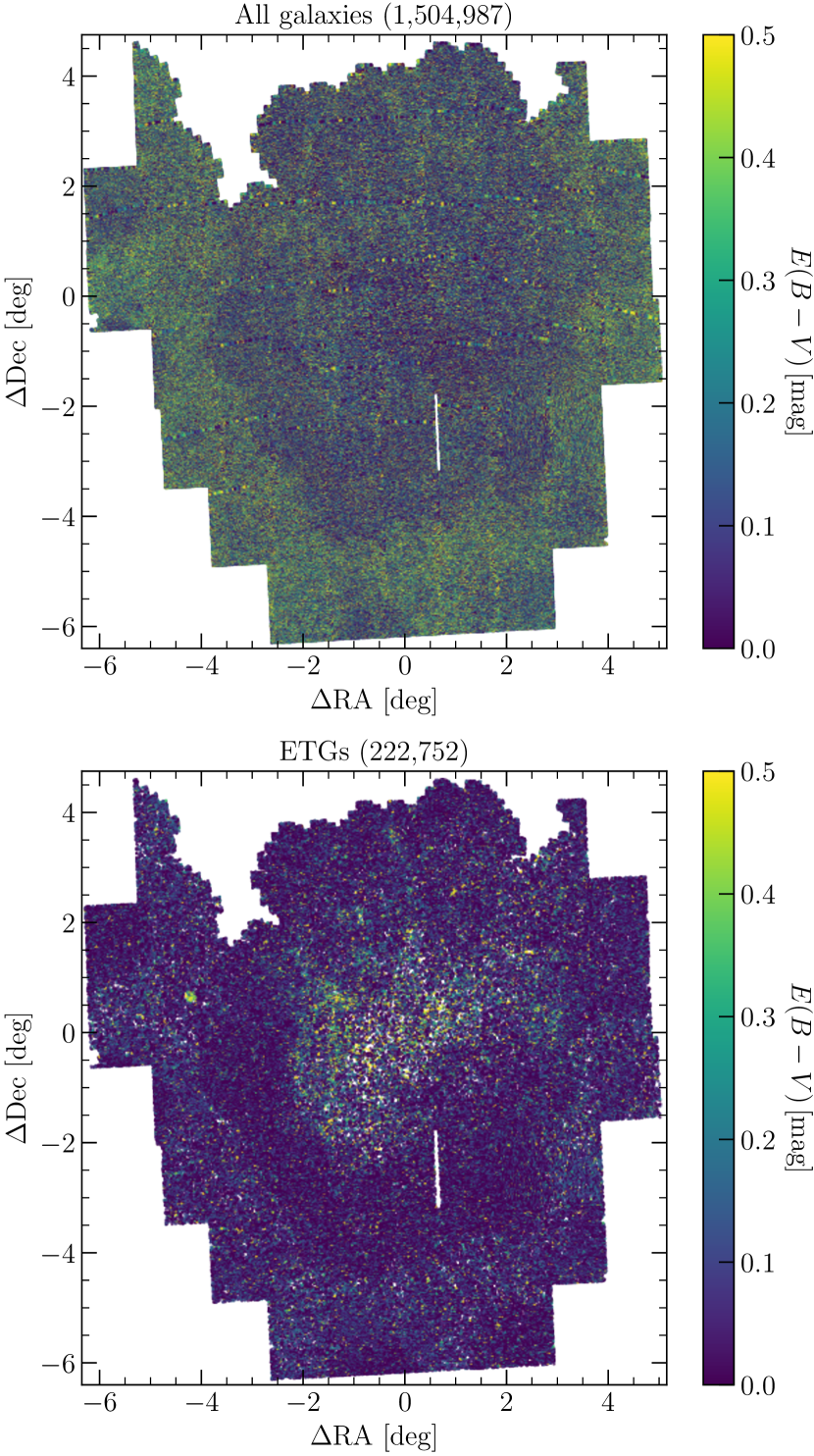
Figure 8: Top panel: Reddening map covering the combined SMASH–VMC footprint created using all objects classified as galaxies by lephare. Bottom panel: As the top panel, but using only objects classified as ETGs.

Fig. 8 shows the reddening map covering $\simeq$ 90 deg² of the LMC based on the 1,504,987 objects classified as galaxies by lephare in the full LMC sample (top panel) in addition to the map created using only the subsample of 222,752 objects classified as ETGs (bottom panel). From Fig. 8 there are two striking observations. First, it is clear that the use of all galaxies (as discussed in Papers I and II) effectively masks the regions where significant amounts of dust intrinsic to the LMC are expected (e.g. along the bar region). This is primarily due to the inclusion of late-type galaxies which are much more numerous than the ETGs and for which the best-fitting template requires additional reddening (including lines of sight through the LMC that do not exhibit significant amounts of reddening), resulting in the systematically higher reddening values across the LMC in the top panel of Fig. 8 compared to the bottom panel. It is only by creating the reddening map using ETGs (with low levels of intrinsic dust themselves) that regions of high internal reddening in the LMC become apparent. Second, there is an obvious difference between the regions that include $u$-band data and those that do not (see also Section 2.4.1). Comparing Figs. 1 and 8 it is evident that the regions for which $u$-band data are available tend to exhibit lower levels of reddening (except for the central regions) than regions for which these data are not available. The enhanced reddening surrounding the galaxy beyond $3-4$ deg from the centre might therefore not be real. The MW correction is applied directly to the LAMBDAR fluxes prior to the SED-fitting (see Sec. 2.3). As we only allow the additional reddening to vary from $0.0-0.5$ in $E(B-V)$, there are no ETG galaxies for which the intrinsic reddening is negative.

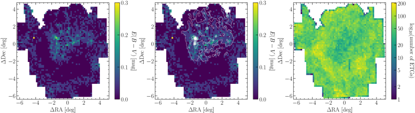
Figure 9: Left panel: $10\times 10$ arcmin² resolution reddening LMC map using objects classified as ETGs. Middle panel: As the left panel, but with the IRAS 100 $\mu$m dust emission contours overlaid to aid the reader in terms of where enhanced levels of reddening (due to the presence of dust) are expected across the LMC. Right panel: Number density of ETGs.

Fig. 9 shows a $10\times 10$ arcmin² resolution reddening map using the same objects as shown in the bottom panel of Fig. 8 to better illustrate large-scale patterns/features across the LMC. Each bin corresponds to the median of the best-fitting $E(B-V)$ values and the median number of ETGs per bin is 63. Of 3348 bins covering the combined SMASH–VMC footprint of the LMC, only 52 (2 per cent) have fewer than 10 ETGs per bin and these are distributed around the outskirts, although there is an obvious dearth of ETGs also associated with the vertical stripe shown in Fig. 8 resulting from missing VMC data (see the right-hand panel of Fig. 9). It is also clear from Fig. 9 that there are fewer ETGs in the central regions of the LMC, which are more heavily affected by crowding. Across the central regions of the LMC we find that the minimum number of ETGs in any given bin is 18, which although significantly lower than the median of 63 across all bins, does not appear to be systematically affected [in terms of the $E(B-V)$ value] with respect to the median $E(B-V)$ values in the neighbouring bins (for which the number of ETGs ranges from 20 to 82). However, there might be ETGs missing due to high extinction regions, which will introduce a bias towards lower extinctions, since both crowding and extinction increase inwards.

Also apparent from Fig. 9 is the excellent agreement between the regions of enhanced reddening across the central regions of the LMC and the regions that exhibit emission at longer wavelengths due to the presence of dust (as traced by the IRAS 100 $\mu$m emission contours). The regions of the LMC for which SMASH $u$-band data are available completely cover these regions and so the transition from regions where we expect dust to be present to regions where little/no dust is present is reflected in the reddening values determined from the ETGs. Farther from the LMC centre, where no $u$-band data are available (except for some small isolated regions; see Fig. 1) enhanced levels of reddening again become noticeable. Given the lack of $u$-band data in these regions, and the aforementioned agreement between the ETG-determined regions of enhanced reddening and far-IR emission, one should treat the absolute reddening values in these outer regions of the LMC with caution [although they are, to within the uncertainties on the median $E(B-V)$, also consistent with zero intrinsic reddening].

The use of ETGs to trace the intrinsic reddening of the LMC has been shown to reproduce the pervasive enhanced levels of reddening across the LMC bar region that we know are present from existing far-IR observations (see e.g. Chastenet et al., 2017 and references therein). In addition, there are several isolated regions for which the median reddening is further enhanced, with respect to this low-level pervasive enhancement. These enhancements coincide with well-known star-forming regions throughout the bar (e.g. N44, N105, N113, N120, N144, and N206, as well as the Tarantula Nebula and the molecular ridge south of 30 Doradus) as well as overdensities observed in morphology maps based on young stars. Interestingly, highest median reddening [$E(B-V)=0.35$ mag; $\Delta$RA $\simeq$ –4.2, $\Delta$Dec $\simeq$ 0.7 deg] lies far from the LMC bar in a region that is not actively forming stars and for which there are no hints of enhanced far-IR emissions in the IRAS 100 $\mu$m data (see Fig. 9).

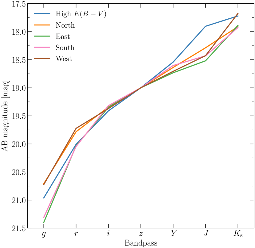
Figure 10: Comparison of median SEDs for all ETGs in the bin with the highest intrinsic reddening (see text) as well as neighbouring bins to the north, south, east and west.

It should be noted, that this region of the combined SMASH–VMC footprint lacks $u$-band data and so that could partly be responsible for the anomalous reddening value. However, the lack of other such enhancements in regions that lack $u$-band data suggests this is not the sole reason. Furthermore, the number of ETGs used to compute the median reddening is almost identical to the median across the whole LMC (cf. 61 and 63) and there is a clear overdensity of ETGs with higher than average reddening values (see Fig. 8). Fig. 10 shows a comparison’s between the median SED for all ETGs in the bin with the highest intrinsic reddening and the ETGs in the neighbouring bins to the north, south, east and west. Note that for comparison sake we have normalised all SEDs to a $z$-band magnitude of 19.0 mag. Although there is very good agreement between the SEDs across most of the optical/near-IR regime, there is a clear difference in the $J$-band regime, such that the median SED of the ETGs in the high reddening bin is $\simeq$ 0.5 mag brighter than those in the neighbouring bins. This difference is likely the reason behind the anomalously high intrinsic reddening in this particular bin and may be related to a higher level of background substructure observed in the VISTA $J$-band deep stack images covering this region of the sky.

The majority of the bins covering the combined SMASH–VMC footprint have $E(B-V)=0.0$ mag [$E(B-V)_{\rm{mean}}=0.06$ mag] and a median uncertainty of $\sigma_{E(B-V)_{\rm{med}}}=0.09$ mag. For bins with only a single ETG, or for which all best-fitting reddening values are identical, we assume an uncertainty of 0.05 mag corresponding to the spacing implemented in the SED process. Table 4 lists the median reddening values, standard deviations and the number of ETGs in each bin across the LMC footprint.

Table 4: Reddening values derived from ETGs within 3348 bins across the LMC. The full table is available as Supporting Information.

$\Delta$RA (J2000.0)	$\Delta$Dec. (J2000.0)	$E(B-V)_{\mathrm{med}}$	$\sigma_{E(B-V)_{\rm{med}}}$	No. ETGs
deg	deg	mag	mag
$-2.54675$	$-6.21777$	0.050	0.089	77
$-2.38055$	$-6.21777$	0.050	0.074	58
$-2.21435$	$-6.21777$	0.100	0.065	66
$-2.04816$	$-6.21777$	0.050	0.059	47
$-1.88196$	$-6.21777$	0.050	0.071	68
$-1.71576$	$-6.21777$	0.000	0.105	52
$-1.54957$	$-6.21777$	0.025	0.109	56
$-1.38337$	$-6.21777$	0.000	0.083	58
$-1.21718$	$-6.21777$	0.000	0.080	90
$-1.05098$	$-6.21777$	0.000	0.089	63

4 Discussion

This study produced a map of the total intrinsic reddening of the LMC for a $\simeq$ 90 deg² region covered by both the SMASH and VMC surveys. Using ETGs we have demonstrated the ability to identify regions with enhanced levels of reddening that coincide with regions of enhanced far-IR emission. We proceed to compare our reddening map with maps created from other tracers to determine how well the various tracers agree in terms of both the line-of-sight reddening values as well as dust distribution morphology. As with the comparison in Paper II, in the figures presented below we do not make any correction for the difference in the volume sampled between the reddening map based on ETGs and those based on various LMC stellar components. If necessary, we remove the foreground MW reddening from the literature maps following the same prescription as described in Section 2.3. The SFD98 $E(B-V)$ values have been demonstrated to be overall systematically overestimated (see e.g. Yuan et al., 2013) and so whilst their use to de-redden the lambdar fluxes was justified (as the extinction coefficients already accounted for this overestimation), their use to de-redden the reddening values in the literature maps would result in us effectively overestimating the foreground MW reddening, and as such adopt a scaling of 0.86 to reflect the recalibration of Schlafly & Finkbeiner (2011).

4.1 Literature LMC reddening maps

4.1.1 Inno et al. (2016)

As part of our comparison in Paper II we adopted the Cepheid sample of Joshi & Panchal (2019), however here we instead adopt that of Inno et al. (2016). Although the reddening values are in very good agreement, the latter covers a larger area of the LMC disc and is thus preferable as a comparison data set. Inno et al. (2016) studied the structure of the LMC disc using multi-wavelength observations of Classical Cepheids (from the $V$-band in the optical to the $W1$-band in the mid-IR). As part of this study, Inno et al. (2016) used a multi-wavelength fitting of the reddening law to the apparent distance moduli to determine the colour excess to individual Cepheids and thus create a reddening map covering $\simeq$ 80 deg² of the LMC disc. For more details regarding the methodology, readers are referred to the works of Freedman, Wilson & Madore (1991) and Gallart, Aparicio & Vilchez (1996) as early examples. Inno et al. (2016) assumed a value of $R_{V}=3.23$, where $R_{V}$ denotes the total to selective absorption, as part of their reddening analysis and provide the individual reddening values in the form of $E(B-V)$. The highest median reddening corresponds to $0.65$ mag whereas the mean reddening corresponds to $0.02$ mag.

4.1.2 Choi et al. (2018)

Choi et al. (2018) used $g$- and $i$-band data from SMASH to create a $2.67\times 2.67$ arcmin² resolution reddening map covering $\simeq$ 165 deg² of the LMC from a sample of $\sim$ 2.2 million RC stars. As opposed to simply adopting a given intrinsic RC $g-i$ colour, Choi et al. (2018) instead measured the intrinsic colour radial profile using a “clean” RC sample based on regions in the outskirts of the LMC that are essentially dust-free (see their figs. 4 and 7). The stars in these regions were de-reddened using the SFD98 dust map before constructing the intrinsic colour radial profile. The reddening map was created by comparing the observed $g-i$ colour map and the intrinsic $g-i$ colour map which is based on the intrinsic colour radial profile. Note that the radial profile only covers an angular distance range of 2.7 to 8.5 deg (from the LMC centre) and thus Choi et al. (2018) adopted the intrinsic RC colour at a distance of 2.7 deg for the innermost regions ($<2.7$ deg) and similarly the intrinsic RC colour at a distance of 8.5 deg for the outermost regions ($8.5-10.5$ deg). To convert the $E(g-i)$ values presented in the Choi et al. (2018) reddening map, we use the extinction coefficients listed in eq. 1 of Paper I to yield $E(g-i)=1.617\times E(B-V)$. In the resulting map the highest median reddening is of $0.35$ mag and the mean reddening is of $0.02$ mag.

4.1.3 Skowron et al. (2021)

Skowron et al. (2021) used $V$- and $I$-band data from OGLE-IV (Udalski, Szymański & Szymański, 2015) to create a reddening map covering $\simeq$ 180 deg² of the LMC using RC stars. The resolution of the reddening map varies from $1.7\times 1.7$ arcmin² in the central regions to $\simeq$ $27\times 27$ arcmin² in the outer regions. Skowron et al. (2021) determined an intrinsic RC $V-I$ colour radial profile by de-reddening the observed RC colours using the SFD98 dust map. Note that the authors exclude the central 4.1 deg radius region around the LMC centre due to the incorrect reddening values provided by the SFD98 dust maps as well as some outer regions due to spurious RC colour measurements (see their section 4 for details). To estimate the intrinsic RC colour in the inner and outer regions, Skowron et al. (2021) used spectroscopic information from Apache Point Observatory Galactic Evolution Experiment (APOGEE) spectra of red giant stars taken from Nidever et al. (2020) to first calculate the LMC metallicity gradient and then a sample of intermediate-aged (3–9.5 Gyr) clusters to determine the variation of the intrinsic RC colour as a function of metallicity. These two relations are then combined to provide an intrinsic colour change as a function of distance from the LMC centre of –0.002 mag deg^-1 that is used to calculate the intrinsic RC colour in the aforementioned excluded regions (see their fig. 13). $E(V-I)$ values are converted into $E(B-V)$ using the relation from Cardelli, Clayton & Mathis (1989). We find a highest median reddening of $0.28$ mag and a mean reddening to $0.01$ mag.

4.1.4 Cusano et al. (2021)

Cusano et al. (2021) used a combination of near-IR time-series photometry from the VMC and optical light curves from OGLE-IV to study the structure of the LMC as traced by $\simeq$ 29,000 RR Lyrae stars. As part of this analysis, they also determined optical $E(V-I)$ reddening values by comparing the observed colours of these stars to their intrinsic colour (based on an empirical relation connecting the intrinsic colour of the star to its $V$-band amplitude and period; see also Piersimoni, Bono & Ripepi, 2002). Although Cusano et al. (2021) do not provide the individual $E(V-I)$ reddening values, they do provide the individual $K_{\rm{s}}$-band extinction values (see their table 3) and so we convert these to $E(B-V)$ values using the extinction coefficient listed in eq. 1 of Paper I [$A_{K_{\rm{s}}}=0.308\times E(B-V)$]. The highest median reddening corresponds to $0.67$ mag and the mean reddenign to $0.02$ mag.

4.1.5 Utomo et al. (2019)

Utomo et al. (2019) homogeneously reanalysed archival far-IR maps from Herschel in four Local Group galaxies (including the LMC at $\sim$ 1 arcmin resolution) by fitting the SED of dust from 100 to 500 $\mu$m with a modified blackbody emission model (see Chiang et al., 2018 for details regarding the model fitting). For our purposes, we are interested in the dust mass surface density, $\Sigma_{\rm{d}}$, returned by the best-fitting model, as this can then be converted into $E(B-V)$ which can then be directly compared to the values we derive using ETGs. IR emission across these wavelengths primarily captures emission from relatively large dust grains that are in thermal equilibrium with the local radiation field, and represent the bulk of the total dust mass. The smaller grains however contribute to the reddening because of their surface to volume ratio. We note that the dust map of the LMC adopted in this work (Chiang et al. priv. comm.) differs slightly from that calculated in Utomo et al. (2019) in two small ways. First, whereas Utomo et al. (2019) adopt a simple power law (see their eq. 5), the dust map included here instead uses a broken power law (see eqs. 2 and 3 of Chiang et al., 2021) as this yields a better fit to the data (see Chiang et al., 2018). Second, as a result of modifying the form of the fit, the emissivity at 160 $\mu$m (the reference wavelength in Utomo et al., 2019 and which is determined by calibrating the models to the Milky Way cirrus where the dust mass is known, see e.g. Jenkins, 2009; Gordon et al., 2014) increases slightly to $\kappa_{160\,\mu\rm{m}}=20.73\pm 0.97$ cm² g^-1 (cf. $18.7\pm 0.6$ cm² g^-1 in Utomo et al., 2019).

In Paper II (see section 4.1.3) we demonstrated a method to convert $\Sigma_{\rm{d}}$ to $E(B-V)$ following the formalism of Whittet (2003) and for which it was necessary to make assumptions regarding the values of the $V$-band extinction efficiency factor, $Q_{V}$, as well as the radius, $a$, and density, $\rho_{\rm{d}}$, of the dust grains. Here we adopt a simpler, albeit model-dependent, approach using the following conversion (see Draine et al., 2014 and references therein):

$$A_{V}=0.7394\left(\frac{\Sigma_{\rm{d}}}{10^{5}\,\mathrm{M_{\odot}/kpc^{2}}}\right)\,\mathrm{mag}$$ (1)

and then convert $A_{V}$ into $E(B-V)$ as in (Cardelli et al., 1989). Despite the different methods to convert $\Sigma_{\rm{d}}$ into $E(B-V)$, the median difference in the resulting $E(B-V)$ values is only $\Delta E(B-V)_{\rm{med}}=0.004$ mag. Furthermore, significant differences (greater than the 0.05 mag level) affect only 1 per cent of the total number of pixels covering the area of the LMC observed by Herschel and coincide with the most intense regions of star formation. As in Paper II, we do not need to subtract the foreground MW contribution as this has already been accounted for as part of the SED modelling.

4.1.6 Mazzi et al. (2021)

Mazzi et al. (2021) used near-IR VMC data to determine the SFH across $\simeq$ 96 deg² of the LMC with a spatial resolution of 0.125 deg². The derivation of the SFH consists of determining the linear combination of partial models that best fit the observed $K_{\rm{s}},Y-K_{\rm{s}}$ and $K_{\rm{s}},J-K_{\rm{s}}$ colour–magnitude Hess diagrams. These models include the effects of extinction, and so by finding the best-fitting combination of models, Mazzi et al. (2021) determined a representative “mean” $V$-band extinction for each subregion. We transform $A_{V}$ into $E(B-V)$ following Cardelli et al. (1989) [$A_{V}=3.1\times E(B-V)$]. Note that we only adopt the $A_{V}$ values resulting from the $K_{\rm{s}},J-K_{\rm{s}}$ fits due to possible issues with the absolute $Y$-band calibration. Due to SFH analysis being performed on discretised regions across the LMC, we are unable to compare this reddening map to the map based on ETGs at a resolution of $10\times 10$ arcmin². To facilitate a comparison, we will degrade the resolution of the ETG reddening map and discuss this map separately (see Section 4.2).

4.2 Comparing different reddening tracers

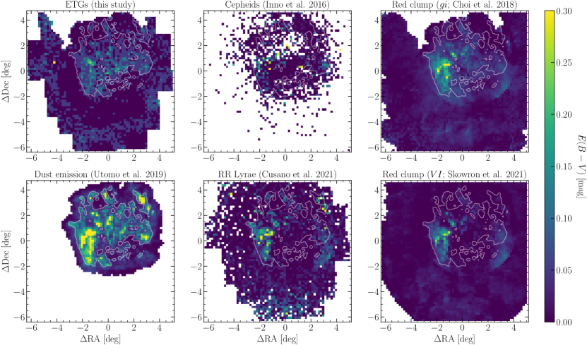
Figure 11: $10\times 10$ arcmin² resolution reddening maps of the LMC. Each panel refers to a different literature source/tracer. The contour in each panel represents the low-level pervasive dust associated with the central regions of the LMC as traced by the IRAS 100 $\mu$m emission. Note that the colour bar range has been limited to $0\leq E(B-V)\leq 0.3$ mag to better illustrate low-level features within the maps. Note also that the ETG extinctions should be roughly twice that of the Cepheids, RR Lyrae and RC values since the latter do not sample the full path through the LMC.

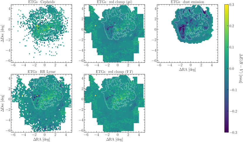
Figure 12: As Fig. 11, but showing a $10\times 10$ arcmin² resolution differential reddening maps of the LMC, such that $\Delta E(B-V)=E(B-V)_{\mathrm{ETG}}-E(B-V)_{\mathrm{tracer}}$. Note that the colour bar range has been limited to $-0.3\leq E(B-V)\leq 0.3$ mag to better illustrate low-level features within the maps.

Fig. 11 shows the comparison between the LMC reddening map based on ETGs and the other maps resampled onto the same $10\times 10$ arcmin² resolution. The majority of the maps used in our comparison have higher spatial resolutions than that shown in Fig. 11 and so some small-scale features (of the order of tens of pc in size) will be masked. Despite this resampling, any large-scale features present in the maps will be retained and evidenced in Fig. 11. In addition, Fig. 12 shows the difference between the reddening map based on ETGs and the literature maps such that $\Delta E(B-V)=E(B-V)_{\mathrm{ETG}}-E(B-V)_{\mathrm{tracer}}$.

Whilst the various reddening tracers shown in Fig. 11 all exhibit enhanced levels of intrinsic reddening in some areas across the central regions of the LMC (in particular the Tarantula Nebula and the molecular ridge south of 30 Dor), not all are consistent with the morphology of the low-level pervasive dust emission as traced by the IRAS 100 $\mu$m emission. In particular, we see clear differences between the stellar tracers (Cepheids, RR Lyrae and RC) and those that sample ETGs and far-IR emission. However, the dust emission or the Cepheids maps are likely very highly biased (the former by heating sources, the latter by being near regions of star formation) and therefore not appropriate to compare to the values presented here. The older stars are more likely to be representative of random lines of sight (modulo the factor of two difference).

Reddening values derived from pulsating stars (Cepheids and RR Lyrae stars) are lower in the central region of the galaxy (at the location of the bar) compared to regions east, west and north of it. These tracers follow a spatial distribution typical of young and old stars, respectively, with most of them located within a structure of a few kpc along the line of sight (e.g. Inno et al., 2016; Cusano et al., 2021). The lower level of reddening suggested by pulsating stars in the bar region compared to ETGs could be explained by the predominant location of these sources in front of the dust rather than behind it. This is however unlikely because both types of variables occupy the entire thickness of the galaxy. Whilst the sample of Cepheids and RR Lyrae stars are highly complete they suffer from incompleteness/blending, due to crowding, in the central regions (e.g. Holl et al., 2018). This effect reduces the amplitude of variation with respect to that of isolated stars, and makes the stars redder which corresponds to a lower reddening towards them (see eqn. 2 of Cusano et al., 2021). The western edge of bar is consistently reddened in all maps, but the continuous extension towards the south is only prominent in the maps derived from RR Lyrae and RC stars. The latter shows also reddening in the central bar region, especially in the map from Choi et al. (2018). RC stars sample the same range of distances as RR Lyrae stars, but are significantly more numerous which may explain their capability to trace reddening across a larger volume.

Similarly to our findings, the middle of the northern arm (a structure parallel to the bar) shows the largest reddening values compared to the other regions within it. Maps extending to the outer regions confirm enhanced reddening values in the south. In our map, the region of 30 Dor and of the molecular ridge south of it appear as reddened as the bar region. This may be a selective effect due to a lack of ETGs in regions of high extinction and/or crowding introducing a bias to lower reddening values (see also Sect. 3). Both effects do influence the molecular ridge region whereas crowding is the dominant effect in the bar region.

The differential reddening maps imply that, by sampling the full line of sight of the LMC, the intrinsic reddening values inferred from the background galaxies are on average higher than those inferred from stellar tracers. If we allow for a factor of 2 difference to account for this depth effect and consider that the median uncertainty on the reddening is of $\sigma_{E(B-V)_{\mathrm{med}}}=0.09$ mag, we find that our map is consistent with those from RC stars for which the highest median reddening differs by $0.19$ mag (Skowron et al., 2021) and $0.26$ mag (Choi et al., 2018), respectively. On the contrary, the highest median reddening for the dust emission exceeds that of our map by $0.50$ mag, for the Cepheids by $0.60$ mag and for the RR Lyrae stars by $0.62$ mag. Note that these values are not shown in Fig. 12 because the reddening scale has been limited to $\pm 0.3$ mag to better illustrate low-level features. The mean reddening differences are however consistent with zero for all tracers.

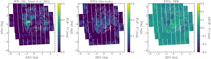
Figure 13: Left panel: Reddening map of the LMC derived from the SFH study by Mazzi et al. (2021). The spatial resolution corresponds to bins of $21.0\times 21.5$ arcmin² whereas the area shown is the same as in Figs. 8, 9 and 11, hence the white space in the south and not all bins shown in the north. The contour represents the low-level pervasive dust associated with the central regions of the LMC as traced by the IRAS 100 $\mu$m emission. Note that the colour bar range has been limited to $0\leq E(B-V)\leq 0.3$ mag to better illustrate low-level features within the maps. Middle panel: As the left panel, but showing the ETG reddening map adopting the spatial resolution of Mazzi et al.. Right panel: As the left panel, but showing the differential reddening map, such that $\Delta E(B-V)=E(B-V)_{\mathrm{ETG}}-E(B-V)_{\mathrm{SFH}}$. Note that the colour bar range has been limited to $-0.3\leq E(B-V)\leq 0.3$ mag to better illustrate low-level features within the map.

The comparison between our reddening map and the map derived from the SFH analysis is shown instead in Fig. 13. In this case, the spatial resolution of each map corresponds to bins of $21.0\times 21.5$ arcmin². The SFH shows the highest reddening values in star forming regions (30 Dor, Constellation III and at the west end of the bar) which are not representative of the line-of-sights we trace in our study. Apart from other localised overdensities comparable to the size of a few bins the overall reddening is low. In particular, the central bar region appears as extinct as the outer regions whereas in our study the bar and the overall inner region of the galaxy appear more extinct than its surroundings. By differentiating the SFH and ETG reddening maps we obtain a rather smooth distribution which agrees within the factor of 2 higher distance sampled by the ETGs. This suggests that a significant fraction of the dust is located beyond the bar sampled by the SFH analysis. The bar region is also affected by extreme crowding and in this region the SFH analysis relies more heavily on RC and RGB stars than on main-sequence turn-off and subgiant stars; these regions are associated to a low likelihood (Mazzi et al., 2021).

To further inspect possible correlations between the ETGs reddening and the reddening derived from the other tracers we plot in Fig. 14 the relation between them. The best fit lines are clearly different from the one-to-one relation, except for the reddening derived from the dust emission which follows a similar trend, but is offset by about 0.5 mag. We already mentioned earlier that despite the influence of heating sources there is a good agreement with the distribution of the low-level pervasive dust emission traced by the IRAS at 100 $\mu$m.

Figure 14: Comparison of the reddening values in the 10$\times$10 resolution ETG reddening map and those of the other reddening tracers. Note that the comparisons only include bins that cover the combined SMASH-VMC footprint of the LMC. The solid line and shaded region in each panel represent the linear best fit and corresponding 67 per cent confidence interval. The dashed line in each panel denotes the one-to-one correspondence between the two reddening tracers.

Figure 15 shows histograms of the distribution of reddening values for the different samples. For all tracers, the peaks of the distributions correspond to reddening values inferior to 0.1 mag. The slope of the distributions towards higher reddening values is however different among the different tracers. It is shallower for the dust emission based reddening than for the stellar ones. The ETG reddening does not show a prominent tail, but rather a wide peak where the distribution of values is confined within about 0.15 mag for the majoirty of the sources.

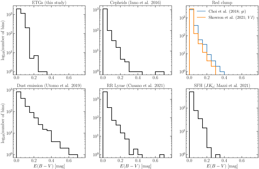
Figure 15: Histograms showing the distribution of reddening values in the 10$\times$10 resolution reddening maps shown in Figs. 11 and 13. Note that the histograms only include bins that cover the combined SMASH-VMC footprint of the LMC.

Figure 16 shows the magnitude of ETGs after applying the reddenign correction. This figure was created in the same way as that described for the reddening map, but instead of taking the median value of all best-fit reddening values in a given bin, we take the median of all extinction corrected J-band magnitudes. Note that the J-band magnitudes are calculated from the LAMBDAR fluxes and corrected for extinction using the relation shown in eqn. 1 of Paper I. We use the J-band magnitude because it is available for almost all ETGs (essentially 100%; 222736 out of 222752 ETGs), whereas for the optical bands we notice a decrease in the number of ETGs with measured fluxes that grows as one moves to bluer bandpasses, e.g. only 49% and 88% of ETGs have measured u- and g-band fluxes, respectively. In the r-, i- and z-bands, we have 97%, 98% and 99% completeness, respectively. The variation of the magnitude of ETGs shows that they sample a different physical scale and therefore a different amount of dust towards the inner and outer regions of the LMC. This is due to the limitation by crowding in the centre and the shallow exposures in the outermost area. More line of sights are needed to describe the likely extinction in these areas compared to that in the intermediate area where the magnitude of ETGs is fairly homogeneous at about J=20.2 mag.

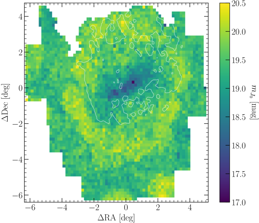
Figure 16: Map of the ETG extinction corrected J-band magnitude ($m_{J_{\mathrm{0}}}$) across the LMC at a resolution of 10$\times$10 arcmin².

5 Summary

In this study, we have determined the total intrinsic reddening across $\simeq$ 90 deg² of the LMC based on the analysis of SEDs of background galaxies. We followed a similar technique as developed in Paper I and extended to the SMC in Paper II. The main steps involved in our procedure and the conclusions are as follows.

• We select $\sim$ 2.5 million background sources from the SMASH and VMC catalogues of the LMC by combining colour-magnitude and morphological criteria. We use lambdar to measure fluxes and construct SEDs from the optical ($ugriz$) to the near-IR ($YJK_{\rm{s}}$).

• We run the lephare $\chi^{2}$ code to fit the SEDs of the objects, which include 21,828 spectroscopically confirmed AGN, and select 252,752 galaxies with low levels of intrinsic reddening. The resulting reddening map reproduces the pervasive enhanced levels of reddening across the LMC bar region with enhancements associated with star forming regions and overdensities traced by young stars.

• The calculated lephare photometric redshifts for 189 AGN are in very good agreement with the spectroscopically determined redshifts ($\Delta z=z_{\rm{spec}}-z_{\rm{phot}}=-0.009$).

• We compare our reddening map with publicly available maps of the LMC. For the inner region, we find good agreement between our map and the distribution of dust emission. The comparison with stellar tracers, however, is more complicated owing to the variations amongst the reddening maps of the various stellar populations. For those showing a significant level of reddening associated with 30 Dor and molecular ridge we find discrepancies. Given the reduced number of galaxies in highly extinguished and crowded regions, it is possible our map is biased towards lower levels of reddening. In contrast, we find agreement with those maps demonstrating reddening in the bar region and in the outskirts of the galaxy. Given a factor of 2 difference, by sampling the full line-of-sight, and the uncertainties in the reddening determinations our map is consistent with maps derived from RC stars. Furthermore, the good agreement with a SFH-based reddening map indicates that a significant fraction of the dust is located beyond the bar.

• We find that the regions lacking $u$-band data, mostly located in the outskirts of the galaxy, sample ETGs similar to those within the same $griz$ magnitude ranges resulting from deep exposures.

In this study, we have extended and improved our technique to measure the total intrinsic reddening of the LMC using background galaxies. The sample of 252,752 ETGs we used may seem small compared to the size of stellar samples adopted for the same purpose, it is however extremely large if one considers that the LMC lies in front of it. Future studies based on large spectroscopic surveys (including surveys using the 4-metre multi-object spectroscopic telescope (4MOST); e.g. Cioni et al., 2019) will provide spectra for hundreds of thousands of background galaxies which will allow us to not only robustly determine their redshifts but also to develop a complementary method to quantify the total intrinsic reddening in the foreground Magellanic Clouds.

Data Availability

The data underlying this study are available in the study and in its online supplementary material. The SMASH survey images used to create the galaxy SEDs are publicly available at the NOIRLab Astro Data Lab (https://datalab.noirlab.edu/). The deep stack VMC images of the LMC will be released in 2022, whereas the individual observations are publicly available at the ESO archive (http://archive.eso.org/cms.html). The galaxy SEDs will be shared on reasonable request to the corresponding author.

References

- Ajello et al. (2020) Ajello M., et al., 2020, ApJ, 892, 105
- Arnouts et al. (2007) Arnouts S., et al., 2007, A&A, 476, 137
- Bell et al. (2019) Bell C. P. M., et al., 2019, MNRAS, 489, 3200 (Paper I)
- Bell et al. (2020) Bell C. P. M., et al., 2020, MNRAS, 499, 993 (Paper II)
- Bellagamba et al. (2012) Bellagamba F., Meneghetti M., Moscardini L., Bolzonella M., 2012, MNRAS, 422, 553
- Bisigello et al. (2016) Bisigello L., et al., 2016, ApJS, 227, 19
- Cardelli et al. (1989) Cardelli J. A., Clayton G. C., Mathis J. S., 1989, ApJ, 345, 245
- Chastenet et al. (2017) Chastenet J., Bot C., Gordon K. D., Bocchio M., Roman-Duval J., Jones A. P., Ysard N., 2017, A&A, 601, A55
- Chen et al. (2022) Chen B. Q., Guo H. L., Gao J., Yang M., Liu Y. L., Jiang B. W., 2022, MNRAS, 511, 1317
- Chiang et al. (2021) Chiang I.-D., et al., 2021, ApJ, 907, 29
- Chiang et al. (2018) Chiang I.-D., Sandstrom K. M., Chastenet J., Johnson L. C., Leroy A. K., Utomo D., 2018, ApJ, 865, 117
- Choi et al. (2018) Choi Y., et al., 2018, ApJ, 866, 90
- Cioni et al. (2019) Cioni M.-. R. L., et al., 2019, The Messenger, 175, 54
- Cioni et al. (2011) Cioni M.-R. L., et al., 2011, A&A, 527, A116
- Cioni et al. (2013) Cioni M.-R. L., et al., 2013, A&A, 549, A29
- Cowley et al. (1984) Cowley A. P., Crampton D., Hutchings J. B., Helfand D. J., Hamilton T. T., Thorstensen J. R., Charles P. A., 1984, ApJ, 286, 196
- Crampton et al. (1997) Crampton D., et al., 1997, AJ, 114, 2353
- Cristiani & Tarenghi (1984) Cristiani S., Tarenghi M., 1984, A&A, 132, 351
- Cross et al. (2012) Cross N. J. G., et al., 2012, A&A, 548, A119
- Cusano et al. (2021) Cusano F., et al., 2021, MNRAS, 504, 1
- de Grijs & Bono (2015) de Grijs R., Bono G., 2015, AJ, 149, 179
- de Grijs et al. (2014) de Grijs R., Wicker J. E., Bono G., 2014, AJ, 147, 122
- De Marchi et al. (2021) De Marchi G., Panagia N., Milone A. P., 2021, ApJ, 922, 135
- Dobrzycki et al. (2005) Dobrzycki A., Eyer L., Stanek K. Z., Macri L. M., 2005, A&A, 442, 495
- Dobrzycki et al. (2002) Dobrzycki A., Groot P. J., Macri L. M., Stanek K. Z., 2002, ApJ, 569, L15
- Draine et al. (2014) Draine B. T., et al., 2014, ApJ, 780, 172
- Duncan et al. (2018a) Duncan K. J., et al., 2018a, MNRAS, 473, 2655
- Duncan et al. (2018b) Duncan K. J., Jarvis M. J., Brown M. J. I., Röttgering H. J. A., 2018b, MNRAS, 477, 5177
- El Youssoufi et al. (2019) El Youssoufi D., et al., 2019, MNRAS, 490, 1076
- Flesch (2021) Flesch E. W., 2021, MNRAS, 504, 621
- Freedman et al. (2020) Freedman W. L., et al., 2020, ApJ, 891, 57
- Freedman et al. (1991) Freedman W. L., Wilson C. D., Madore B. F., 1991, ApJ, 372, 455
- Gallart et al. (1996) Gallart C., Aparicio A., Vilchez J. M., 1996, AJ, 112, 1928
- Geha et al. (2003) Geha M., et al., 2003, AJ, 125, 1
- Gieren et al. (2018) Gieren W., et al., 2018, A&A, 620, A99
- González-Fernández et al. (2018) González-Fernández C., et al., 2018, MNRAS, 474, 5459
- Gordon et al. (2014) Gordon K. D., et al., 2014, ApJ, 797, 85
- Górski et al. (2020) Górski M., et al., 2020, ApJ, 889, 179
- Gouliermis et al. (2014) Gouliermis D. A., Hony S., Klessen R. S., 2014, MNRAS, 439, 3775
- Groenewegen (2018) Groenewegen M. A. T., 2018, A&A, 619, A8
- Haberl et al. (2012) Haberl F., et al., 2012, A&A, 545, A128
- Haschke et al. (2011) Haschke R., Grebel E. K., Duffau S., 2011, AJ, 141, 158
- Holl et al. (2018) Holl B., et al.., 2018, A&A, 618, A30
- Hunter (2007) Hunter J. D., 2007, Computing in Science & Engineering, 9, 90
- Inno et al. (2016) Inno L., et al., 2016, ApJ, 832, 176
- Irwin et al. (2004) Irwin M. J., et al.., 2004, in Society of Photo-Optical Instrumentation Engineers (SPIE) Conference Series, Vol. 5493, Optimizing Scientific Return for Astronomy through Information Technologies, Quinn P. J., Bridger A., eds., pp. 411–422
- Ivanov et al. (2016) Ivanov V. D., et al., 2016, A&A, 588, A93
- Ivezić et al. (2002) Ivezić Ž., et al., 2002, AJ, 124, 2364
- Jenkins (2009) Jenkins E. B., 2009, ApJ, 700, 1299
- Jiang et al. (2007) Jiang L., Fan X., Ivezić Ž., Richards G. T., Schneider D. P., Strauss M. A., Kelly B. C., 2007, ApJ, 656, 680
- Jones et al. (2009) Jones D. H., et al., 2009, MNRAS, 399, 683
- Jones et al. (2001–) Jones E., et al., 2001–, SciPy: Open source scientific tools for Python
- Joshi & Panchal (2019) Joshi Y. C., Panchal A., 2019, A&A, 628, A51
- Kostrzewa-Rutkowska et al. (2018) Kostrzewa-Rutkowska Z., et al., 2018, MNRAS, 476, 663
- Kozłowski et al. (2012) Kozłowski S., et al.., 2012, ApJ, 746, 27
- Kozłowski et al. (2011) Kozłowski S., Kochanek C. S., Udalski A., 2011, ApJS, 194, 22
- Kozłowski et al. (2013) Kozłowski S., et al., 2013, ApJ, 775, 92
- Mazzi et al. (2021) Mazzi A., et al., 2021, MNRAS, 508, 245
- McKinney (2010) McKinney W., 2010, in Proceedings of the 9th Python in Science Conference, van der Walt S., Millman J., eds., p. 51
- Muraveva et al. (2018) Muraveva T., et al., 2018, MNRAS, 473, 3131
- Nayak et al. (2018) Nayak P. K., Subramaniam A., Choudhury S., Sagar R., 2018, A&A, 616, A187
- Nidever et al. (2020) Nidever D. L., et al., 2020, ApJ, 895, 88
- Nidever et al. (2017) Nidever D. L., et al., 2017, AJ, 154, 199
- Norris et al. (2011) Norris R. P., et al., 2011, PASA, 28, 215
- Oliphant (2015) Oliphant T. E., 2015, Guide to NumPy. CreateSpace Independent Publishing Platform, 2nd ed.
- Paturel et al. (2003) Paturel G., Petit C., Prugniel P., Theureau G., Rousseau J., Brouty M., Dubois P., Cambrésy L., 2003, A&A, 412, 45
- Pennock et al. (2021) Pennock C. M., et al., 2021, MNRAS, 506, 354
- Piersimoni et al. (2002) Piersimoni A. M., Bono G., Ripepi V., 2002, AJ, 124, 1528
- Polletta et al. (2007) Polletta M., et al., 2007, ApJ, 663, 81
- Riess et al. (2019) Riess A. G., Casertano S., Yuan W., Macri L. M., Scolnic D., 2019, ApJ, 876, 85
- Riess et al. (2009) Riess A. G., et al., 2009, ApJ, 699, 539
- Ripepi et al. (2017) Ripepi V., et al., 2017, MNRAS, 472, 808
- Ripepi et al. (2019) Ripepi V., Molinaro R., Musella I., Marconi M., Leccia S., Eyer L., 2019, A&A, 625, A14
- Rubele et al. (2018) Rubele S., et al., 2018, MNRAS, 478, 5017
- Salvato et al. (2009) Salvato M., et al., 2009, ApJ, 690, 1250
- Schlafly & Finkbeiner (2011) Schlafly E. F., Finkbeiner D. P., 2011, ApJ, 737, 103
- Schlegel et al. (1998) Schlegel D. J., Finkbeiner D. P., Davis M., 1998, ApJ, 500, 525
- Skowron et al. (2021) Skowron D. M., et al., 2021, ApJS, 252, 23
- Tatton et al. (2021) Tatton B. L., et al., 2021, MNRAS, 504, 2983
- Taylor (2005) Taylor M. B., 2005, in Astronomical Society of the Pacific Conference Series, Vol. 347, Astronomical Data Analysis Software and Systems XIV, Shopbell P., Britton M., Ebert R., eds., p. 29
- The Astropy Collaboration et al. (2018) The Astropy Collaboration, Price-Whelan A. M., Sipőcz B. M., Günther H. M., et al., 2018, AJ, 156, 123
- Tinney (1999) Tinney C. G., 1999, MNRAS, 303, 565
- Udalski (2003) Udalski A., 2003, Acta Astron., 53, 291
- Udalski et al. (2015) Udalski A., Szymański M. K., Szymański G., 2015, Acta Astron., 65, 1
- Utomo et al. (2019) Utomo D., Chiang I.-D., Leroy A. K., Sandstrom K. M., Chastenet J., 2019, ApJ, 874, 141
- Wang et al. (1991) Wang Q., Hamilton T., Helfand D. J., Wu X., 1991, ApJ, 374, 475
- Whittet (2003) Whittet D. C. B., 2003, Dust in the Galactic Environment. Bristol: Institute of Physics Publishing, 2nd ed.
- Wright et al. (2016) Wright A. H., et al., 2016, MNRAS, 460, 765
- Yuan et al. (2013) Yuan H. B., Liu X. W., Xiang M. S., 2013, MNRAS, 430, 2188
- Zaritsky et al. (2002) Zaritsky D., Harris J., Thompson I. B., Grebel E. K., Massey P., 2002, AJ, 123, 855
- Zivkov et al. (2018) Zivkov V., et al.., 2018, A&A, 620, A143