Intermittent air invasion in pervaporating compliant microchannels

Abstract

We explore air invasion in an initially water-filled dead-end compliant microchannel containing a constriction. The phenomenon is driven by the pervaporation of the liquid present in the channel through the surrounding medium. The penetration is intermittent, jerky, and characterised by a stop-and-go dynamics as the bubble escapes the constriction. We demonstrate that this sequence of arrest and jump of the bubble is due to an elastocapillary coupling between the air-liquid interface and the elastic medium. When the interface enters the constriction, its curvature strongly increases, leading to a depression within the liquid-filled channel which drives a compression of the channel. As the interface is forced to leave the constriction at a given threshold, due to the ongoing loss of liquid content by pervaporation, the pressure is suddenly released, which gives rise to a rapid propagation of the air bubbles away from the constriction and a restoration of the rest shape of the channel. Combining macroscopic observations and confocal imaging, we present a comprehensive experimental study of this phenomenon. In particular, the effect of the channel geometry on the time of arrest in the constriction and the jump length is investigated. Our novel microfluidic design succeeds in mimicking the role of inter-vessel pits in plants, which transiently stop the propagation of air embolism during long and severe droughts. It is expected to serve as a building block for further biomimetic studies in more complex leaf-like architectures, in order to recover this universal phenomena of intermittent propagation reported in real leaves.

1 Introduction

Due to climate change, severe droughts are gradually more frequent across the globe. Trees are particularly vulnerable to water stresses, as their sap conduction mainly occurs at negative pressure, close to the cavitation threshold. When air penetrates the vessels of a tree, it forms an embolism which can dramatically impair its hydraulic circulation and lead to its death (Tyree & Zimmermann, 2013; Venturas, Sperry & Hacke, 2017), which is one the major threats for the survival of forest for the next decades (Choat et al., 2012, 2018; Brodribb et al., 2020).

Direct observations of embolism in trees have recently been enabled by the development of high resolution imaging like X-ray tomography (Cochard, Delzon & Badel, 2015) or magnetic resonance imaging (Choat et al., 2010; Fukuda et al., 2015). However, the time resolution of those methods is generally insufficient to observe fast embolism propagation. Dynamics of embolism growth is more practical to be directly observed in herbaceous plants (Skelton, Brodribb & Choat, 2017) or in leaves (Brodribb et al., 2016b), due to their slender geometry and/or their relative transparency. Leaves are particularly exposed to air and more prone to exhibit air embolisation during droughts. A systematic study across various species recently revealed via optical imaging that the drying in real leaves is characterised by an intermittent jerky dynamics (Brodribb, Bienaimé & Marmottant, 2016a). These sudden propagations contrast with the smooth flows of sap reported in the absence of air embolisms (Katifori, Szöllősi & Magnasco, 2010). Despite a comprehensive description of the embolism formation dynamics in leaves of many species, an in-depth physical understanding is still missing.

In that purpose, we have carried out biomimetic studies, in order to replicate this phenomenon in microfluidic chips. Biomimetic microfluidics in so-called trees-on-a-chip has already enabled to reproduce key phenomenon of plant hydrodynamics, like vein circulation at negative pressure (Wheeler & Stroock, 2008), leaf transpiration (Noblin et al., 2008), cavitation in inclusions (Vincent et al., 2012; Duan et al., 2012; Vincent & Marmottant, 2017; Bruning et al., 2019), osmotic flows (Jensen et al., 2009) or phloem loading (Comtet et al., 2017). Inspired by the design proposed by Noblin et al. (2008) and based on pervaporation across PDMS as a tool to mimic evapotranspiration of leaves, we explored the dynamics of propagation of air embolism in dead-end microchannels (Dollet et al., 2019). However, drying dynamics was found to be smooth, contrary to the phenomenology reported in real leaves. In our previous studies, channel width was taken constant (Dollet et al., 2019, 2021), or slowly varying (Chagua Encarnación, Marmottant & Dollet, 2021). In reality, there are pits between sap-conducting cells in trees which are considered to be at the origin of the resistance to embolisation in wood vessels (Cochard, Cruiziat & Tyree, 1992). Those submicron porous membranes separate neighboring vessels and act as passive valves preventing air bubbles to penetrate further in the network due to capillarity. However, under severe drought, the pressure within the hydraulic network can be so low that air embolism manage to pass through the pits and invade very suddenly the network. The compliance of the hydraulic network of trees, i.e. the change of volume of its channels and neighboring cells in response to a pressure change, is considered as an important feature during air embolism formation (Hölttä et al., 2009), but live observations are still missing.

In microfluidics, numerous studies have investigated the deformation of compliant microchannels due to hydrodynamic forces (Holden et al., 2003; Gervais et al., 2006; Hardy et al., 2009; Christov et al., 2018) in pure one-phase flows. Furthermore, when two phases are transported in a compliant microchannel, the capillary forces exerted at the fluid-fluid interface can substantially deform the walls, a phenomenon referred to as elasto-capillarity (Roman & Bico, 2010). It can lead to complex couplings between two-phase flows and compliant walls (Heil & Hazel, 2016; Juel, Pihler-Puzović & Heil, 2018), as for viscous fingering instabilities (Pihler-Puzović et al., 2012, 2013) or for the propagation of air fingers in rectangular compliant microchannels where highly non-linear dynamics were reported (Ducloué et al., 2017b, a; Fontana et al., 2021). Those latter considerations are of primary importance for numerous biological flows (Heil & Hazel, 2011), in particular in collapsed lungs (Grotberg, 1994; Grotberg & Jensen, 2004; Heil, Hazel & Smith, 2008).

In this paper, we consider the physical effects of a single constriction inside a compliant channel of otherwise constant width, in order to mimic the role of pits in plants. The water, initially present in the vessel, gradually pervaporates through the surrounding medium, a phenomenon replicating the effect of evapotranspiration in real leaves. As the air bubble (or air embolism) grows within the channel and penetrates the constriction, we unravel a stop-and-go dynamics, which may be the building block of the intermittent drying dynamics in leaves. We show that this highly non-linear dynamics is generated by the elasto-capillary coupling between the compliance of the channel and the interface curvature, forced to sustain large changes due to the constriction, thereby inducing substantial changes of the capillary pressure within the liquid-filled part of the channel.

In a first part, we describe the experimental materials and methods used in this study (section 2). We then describe extensively the dynamics of propagation of the air embolism induced by pervaporation, recalling the smooth dynamics in the absence of constriction (section 3.1), contrasting with the stop-and-go induced by the constriction (section 3.2). We associate this dynamics with observations of the deformation of the channels via confocal imaging (section 3.3), and show that the deformation results from an elasto-capillary coupling between the meniscus in the constriction and the deformable channel (section 3.4), in agreement with experiments realised replacing water by ethanol (section 3.5) and with a volume conservation check comparing macroscopic experiments and confocal imaging (section 3.6). We then reinforce the validity of this physical mechanism by depicting the influence of the channel geometry on two key variables of this stop-and-go dynamics: the length of the jump (sections 4.1, 4.2 and 4.3) and the time of residence of the interface inside the constriction (section 4.4). We also describe the dynamics of the sudden propagation of the air embolism past the constriction, and compare it with theoretical predictions (section 5). In a last part, we summarise our findings and propose connections with other fields as well as perspectives for future studies (section 6).

2 Materials and methods

2.1 Photolithography

The channels are made by photolithography. A SU8 resin (provided by Gersteltec) is spin-coated on a silicon wafer, at a thickness $h$. By photolithography, the negative pattern of the channels is cured by UV-light through a mask (provided by Selba company). The uncured resin is then washed out using propylene glycol methyl ether acetate. After a final bake of the silicon wafer at 200^∘C, our textured surface is ready to use as a mold.

2.2 PDMS preparation

In order to make our biomimetic transpirating leaves, we use polydimethylsiloxane (Sylgard^TM 184, from Dow company), a silicone-based elastomer. We mix a mass fraction of $10\%$ of curing agent and 90$\%$ of base. After an energic stirring, the mixture is degassed under vacuum. After about $60$ min of degassing, we spin-coat $2.5$ mL of the mixture on the textured silicon surface ($10$ s at $500$ rounds per minute (rpm) and $40$ s at a speed varying between $700$ and $2000$ rpm depending on the desired thickness $H$). The spin-coated liquid film is then let at rest during $1$ h in order to have a homogeneous thickness by capillary levelling. Finally, the samples are put in an oven at $65^{\circ}$C during $24$ h (or $1$ h depending on the protocol).

2.3 Channel formation and filling with water

After curing of the PDMS, the samples are detached from the textured silicon wafer, and gently deposited on a plasma-treated glass slide. The channels are full of air, and we fill them by water using the following procedure. With a scalpel, we create a wide cut enabling a direct connection between the channel entrance and the outside. The samples are then plunged in a tank of deionised water (resistance of about $18$ M$\Omega$) and put in a vacuum chamber during two hours, such that water gradually replaces the air inside the microchannels.

2.4 Channel design

As represented in figure 1, our biomimetic vessel is composed of two channels of length $L_{\mathrm{in}}=2$ mm and $L_{\mathrm{out}}$ (varying between $900\>\mathrm{\mu}$m and $18$ cm), of respective width $w_{in}=200\>\mathrm{\mu}$m and $w_{\mathrm{out}}$ (varying between $100$ and $450\>\mathrm{\mu}$m). The two channels have a height $h$ (varying between $11$ and $100\>\mathrm{\mu}$m), and are connected by a constriction of length $l_{c}=1$ mm, width $w_{\mathrm{p}}$ (varying between $5$ and $50\>\mathrm{\mu}$m) and height $h$. The total thickness of the PDMS medium is $H$ and typically varies between $56$ and $154$ $\mu$m across experiments. The thickness of the PDMS membrane separating the top of the channels and the external air is denoted $\delta=H-h$ and varies between $10$ and $79$ $\mu$m across experiments.

2.5 Meniscus tracking

In order to record the global displacement of the embolism, we mounted a camera (Pike, from Allied Vision Technologies) on a microscope (magnification varying between $\times 3$ and $\times 5$), and we recorded the position of the meniscus with an acquisition speed varying between 0.1 and 2.5 frames per second (fps). The position of the meniscus is then tracked using the “reslice” function of the free software ImageJ/Fiji.

In order to record the temporal evolution of the interface at the moment of the sudden jump, we mounted a high speed camera (Phantom Miro M$310$) on a microscope (magnification varying between $\times 6.4$ and $\times 8$) with an acquisition speed varying between $400$ and $1000$ fps.

2.6 Confocal imaging

A mass of $1$ mg of sulforhodamine B (a fluorescent dye) was dissolved in 500 mL of deionised water. The solution was then used to fill our channels, following the protocol detailed in section 2.3. Fluorescent-water-filled microchannels were put under a laser-induced fluorescence confocal microscope (TCS SP8 from Leica Microsystems), and enlighted at a wavelength $\lambda=561$ nm. We used a $\times 40$ lens with immersion oil, connected to a photomultiplicator in the wavelength range $[575;\>660]$ nm. The pixel size in our experiments was set at about $200$ nm. We performed $z$-scans of our samples of typical vertical steps $1$ $\mu$m, thereby obtaining images of the channel cross-section (see later figure 4b) every 22 s. These images (see later figure 4b) were then analysed by standard image analysis techniques. As a word of caution, notice that sulforhodamine accumulates at the channel boundary and defines a thick bright line, which limits the precision of the measurement of the cross-section and the channel thickness. In particular, we shall see later (in section 3.3) that both these parameters are slightly overestimated, without consequences on their relative variations along time and space, which will be the quantities of interest.

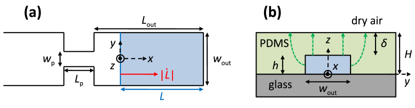
Figure 1: Sketch of the channel (not to scale): (a) top view, (b) side view across the channel. The top view shows the single constriction of length $L_{\mathrm{p}}$ and width $w_{\mathrm{p}}$ inside the channel of width $w_{\mathrm{out}}$. The exit channel, i.e. the channel portion after the constriction, has a length $L_{\mathrm{out}}$. A meniscus, depicted as a blue line across the channel, separates the water-filled part of the channel (right of the meniscus, blue shade in both panels) of length $L$ from the air-filled part (left of the meniscus). The velocity of the meniscus $|\dot{L}|$ is indicated with a red arrow in panel (a); the meniscus motion is due to the loss of water induced by a pervaporation flux across PDMS, sketched by the green dotted arrows in panel (b).

3 Experimental description of the air-finger propagation

We start by considering a reference experiment, whose dynamics is representative of that of all other experiments presented in this paper. The time evolution of the water length $L$ is plotted in figure 2. It shows sharp variations: the meniscus first advances at almost constant speed in the entrance channel, before reaching the constriction entrance, where it stops for about $200$ s. It then accelerates inside the constriction, before a second stop at the constriction exit, for about $250$ s. It then suddenly jumps forwards over a length $L_{\mathrm{jump}}$ of about 1 mm inside the exit channel, at a time denoted $t_{\mathrm{jump}}$, before recovering a smooth dynamics in the exit channel characterised by a progressive deceleration. We supply as Supplementary Material a movie showing the whole process. We study more in details this smooth dynamics in section 3.1, then focus on the constriction-induced sharp variations in section 3.2 and propose physical interpretations in sections 3.3, 3.4, 3.5 and 3.6.

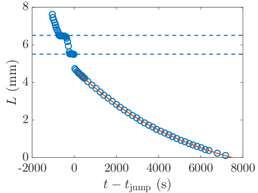
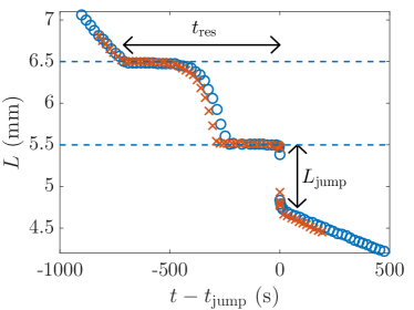
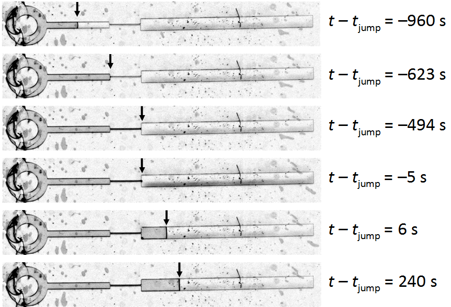
Figure 2: (a) Plot of the water length $L$ as a function of time $t-t_{\mathrm{jump}}$ in a channel of geometrical parameters $L_{\mathrm{out}}=5.5$ mm, $L_{\mathrm{p}}=1$ mm, $w_{\mathrm{out}}=390~{}\mu$m, $w_{\mathrm{p}}=30~{}\mu$m, $h=65~{}\mu$m and $H=95~{}\mu$m, for a relative humidity $\mathrm{RH}=0.25$. The time $t_{\mathrm{jump}}$ is the instant where the meniscus abruptly jumps inside the exit channel. The curve is a fit by the truncated exponential law (1), with $\tau=5.65\times 10^{3}$ s and $L_{g}=1.71$ mm as fitting parameters. (b) Zoom in the constriction of the experiment presented in panel (a) ($\circ$), and of a second realisation of the experiment ($\times$), recorded with a larger magnification. In panels (a) and (b), the two horizontal dashed lines highlight the location of the constriction. (c) Snapshots of the full channel at various times. Arrows highlight the position of the meniscus separating the water-filled part of the channel (right from the meniscus) from its air-filled part (left from the meniscus).

3.1 A smooth dynamics in the absence of constriction

The smooth deceleration of the meniscus occurring after the jump in the exit channel echoes the pervaporation-induced drying dynamics in single channels of constant width studied by Dollet et al. (2019). We remind that this dynamics is driven by the loss of water within the channel due to pervaporation through the water-permeable PDMS walls. There are two contributions to the pervaporation flux $Q$: a diffusion flux, denoted $Q_{\ell}$, from the water–PDMS interface, and an evaporative flux $Q_{g}$ at the meniscus. Since the length of the exit channel is much larger than its width, it is reasonable to neglect end effects on the diffusion flux and to assume that it is simply proportional to the water-filled length: $Q_{\ell}=q_{\ell}L$. Hence, water conservation leads to: $hw_{\mathrm{out}}\dot{L}=-q_{\ell}L-Q_{g}$, from which the following truncated exponential dynamics is predicted:

$$L=(L_{\mathrm{out}}-L_{\mathrm{jump}}+L_{g})\mathrm{e}^{-(t-t_{\mathrm{jump}})/\tau}-L_{g},$$ (1)

using the initial condition $L=L_{\mathrm{out}}-L_{\mathrm{jump}}$ at $t=t_{\mathrm{jump}}$ just after the jump, and defining $\tau=hw_{\mathrm{out}}/q_{\ell}$ and $L_{g}=Q_{g}/q_{\ell}$. Figure 2a confirms that such a truncated exponential fits remarkably well the meniscus dynamics in the exit channel. A similar dynamics is very probably at play also at the entrance channel, but the spatiotemporal range of this part of the dynamics is too narrow to enable for significant fitting.

The two aforementioned fluxes $q_{\ell}$ and $Q_{g}$ have been predicted in Dollet et al. (2019). First, we have:

$$q_{\ell}=D_{P}\bar{c}_{P}^{\mathrm{sat}}(1-\mathrm{RH})\tilde{q}_{\ell}(w_{\mathrm{out}}),$$ (2)

with $D_{P}$ the diffusivity of water in PDMS, $\bar{c}_{P}^{\mathrm{sat}}=7.2\times 10^{-4}$ the mass fraction of water in PDMS at saturation (see Chagua Encarnación, Marmottant & Dollet (2021) for the numerical estimation of this parameter), RH the relative humidity of the outer air, and $\tilde{q}_{\ell}$ the following dimensionless shape factor:

$$\tilde{q}_{\ell}(w)=\frac{w}{\delta}+\frac{2}{\pi}\left[\ln\frac{(H+\delta)h}{\delta^{2}}+\frac{H}{\delta}\ln\frac{H+\delta}{h}\right].$$ (3)

We also use the prediction:

$$Q_{g}=\sqrt{\alpha D_{a}D_{P}hw_{\mathrm{p}}\tilde{q}_{\ell}(w_{\mathrm{out}})},$$ (4)

with $\alpha=0.03$ the Henry constant quantifying the water affinity in PDMS (Harley, Glascoe & Maxwell, 2012), and $D_{a}=2\times 10^{-5}$ m²/s the diffusivity of water vapour in air.

3.2 A stop-and-go dynamics induced by the constriction

Figure 2b shows that the presence of the constriction modifies dramatically the drying dynamics as compared to the smooth dynamics encountered in channels of constant width (Dollet et al., 2019). Moreover, the dynamics is also different to the one studied in Chagua Encarnación, Marmottant & Dollet (2021) for channels of slowly varying width, where the width variations were shown to induce variations of meniscus speed, but not the stick-slip-like motion (arrest followed by jump) evidenced in figure 2b.

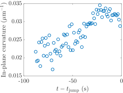
Figure 3: (a) Snapshots of the meniscus at various times within the phase of arrest of the meniscus at the constriction exit; in particular, (i) is the first snapshot where the meniscus is pinned. (b) Plot of the in-plane curvature of the meniscus as a function of time at the end of the arrest phase.

We must mention that some elements of this dynamics are not fully reproducible when the same experiment is run several times. Notably, the arrest times at the constriction entrance and exit, as well as the dynamics within the constriction, vary, as evidenced by the comparison of two different realisations of the experiment in figure 2b. However, the occurrence of the jump at the constriction exit was always observed, and the jump length and arrest time both showed a good reproducibility (of the order of 10%).

To understand the origin of the meniscus arrest, we present magnified snapshots of the meniscus in figure 3a at the constriction exit, which show that the meniscus progressively bulges out during the arrest phase. To quantify this observation, we fitted the meniscus by an arc of circle, and we plot in figure 3b the corresponding in-plane curvature as a function of time during the last 90 s before the jump (at earlier times, the meniscus is not curved enough for its curvature to be accurately measurable): although the measurement is somewhat noisy, this figure shows that the curvature increases and reaches a maximum just before the jump, of order 0.035 $\mu$m^-1, which is very close to $1/w_{\mathrm{p}}=0.033~{}\mu$m^-1.

While the meniscus gets arrested, drying is still proceeding, hence the volume of water in the channel is still decreasing. This suggests that the channel cross-section, in its water-filled part, must decrease during the arrest phase.

3.3 Confocal imaging of the deformation of the channel during the arrest phase

In order to test the hypothesis of a decrease of the cross-section during the arrest phase, we repeated the reference experiment using confocal microscopy to measure the time evolution of the cross-section. To avoid the end effects in the vicinity of the sharp width variation at the constriction exit, we measured the cross-section at a distance 3 mm ahead of the constriction exit. The corresponding data, displayed in figure 4a, show that the cross-section is first roughly constant, then decreases, then increases very rapidly (within the 22 s separating two measurements of the cross-section) to recover the first plateau value. This variation is compatible with the aforementioned dynamics of the meniscus, and with a scenario of drying of the channel at fixed meniscus position but decreasing cross-section, until a critical instant where the meniscus unpins. A fast relaxation ensues, during which the channel quickly recovers its equilibrium cross-section, and where the meniscus jumps forwards at almost constant water volume (neglecting the duration of the jump with respect to the typical pervaporation time).

The confocal snapshot of figure 4b,iv shows that the upper wall remains slightly bent inwards after the jump. This is a signature of a remanent Laplace pressure $p_{\mathrm{rem}}$ when the meniscus is in the exit channel: owing to the wetting conditions of water on PDMS and glass, the meniscus is curved towards the liquid phase (see later figure 7b). Hence, the water has a lower pressure than air, whence the remaining curvature of the upper wall. We shall henceforth denote $S_{\mathrm{rem}}$ the corresponding cross-section, which is thus slightly smaller (of order 5%) than the equilibrium cross-section $S_{0}=hw_{\mathrm{out}}$.

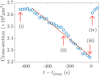
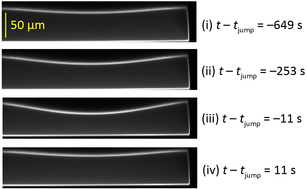
Figure 4: (a) Plot of the cross-section of the channel $S$ as a function of time in a channel of geometrical parameters $L_{\mathrm{out}}=5.5$ mm, $L_{\mathrm{p}}=1$ mm, $w_{\mathrm{out}}=390~{}\mu$m, $w_{\mathrm{p}}=30~{}\mu$m, $h=65~{}\mu$m and $H=95~{}\mu$m. The time here is defined with respect to the instant of the jump $t_{\mathrm{jump}}$. The straight line is a linear fit over the time interval where the cross-section decreases. Arrows with labels refer to the photographs taken with the confocal microscope displayed in panel (b). The boundary of the channel cross-section appears in light shade; notice that a tiny part of the cross-section is cut at the left of the photographs, owing to limitations of the horizontal field of view of the confocal microscope.

The data of figures 3b and 4a suggest that the curvature of the pinned meniscus varies in order for the Laplace pressure to accommodate the decrease in water pressure accompanying the cross-section reduction. To prove this correlation, we performed another experiment based on confocal microscopy, close enough to the constriction exit to simultaneously track both the meniscus shape and the cross-section. Owing to the finite time resolution of the confocal scans, we cannot reconstruct reliably the 3D structure of the meniscus, because it advances significantly between the bottom scan and the top scan. Hence, we present a measurement of the curvature of the meniscus in the horizontal plane located midway between the bottom glass plate and the top PDMS channel wall (henceforth called the in-plane curvature). We plot in figure 5 the cross-section difference with respect to the undeformed case, defined as $\Delta S=hw_{\mathrm{out}}-S$, as a function of the in-plane curvature in the last moments of the arrest phase. This figure shows that, except for an outlier, the two quantities are well correlated by an affine relation, thereby confirming our interpretation.

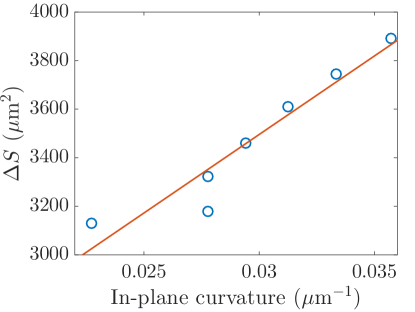
Figure 5: Plot of the cross-section difference of the channel $\Delta S=hw-S$ as a function of the in-plane curvature $\kappa$ of the meniscus in a channel of geometrical parameters $L_{\mathrm{out}}=5.5$ mm, $L_{\mathrm{p}}=1$ mm, $w_{\mathrm{out}}=390~{}\mu$m, $w_{\mathrm{p}}=30~{}\mu$m, $h=50~{}\mu$m and $H=59~{}\mu$m, for the last moments of the arrest phase. The line is an affine fit of the data $\Delta S=c_{1}\kappa+c_{2}$, with fitting parameters $c_{1}=6.5\times 10^{4}~{}\mu$m³ and $c_{2}=1.6\times 10^{3}~{}\mu$m².

Once the meniscus reaches its maximal possible curvature compatible with the geometrical constraints and the contact angles of water on PDMS and glass, the situation becomes unstable, because the Laplace pressure can no longer equilibrate the elastic deformation of the channel, and the meniscus advances rapidly until the channel is fully relaxed. The onset of the jump is therefore an occurrence of a capillary threshold, as encountered in the drainage of Newtonian fluids in porous media (Wilkinson & Willemsen, 1983; Lenormand & Zarcone, 1985; Måløy et al., 1985; Méheust et al., 2002), or in the flow of foams in porous media (Géraud et al., 2016). Hence, the maximal deformation of the channel is correlated, through Laplace pressure, to the maximal curvature of the meniscus. Because of the finite roundness of the corners at the constriction exit, the meniscus shape is a complicated surface, which prevents us from predicting the maximal curvature. However, its order of magnitude is $1/w_{\mathrm{p}}$ (figure 3b), as would be expected for a 2D meniscus pinned on sharp corners, whose maximal possible curvature equals $2/w_{\mathrm{p}}$ when it has the shape of a half circle.

3.4 An elasto-capillary interaction between the meniscus and the channel structure

We shall now analyse the full shape of the channel upper wall as seen in figure 4b. In that experiment, the upper wall has a thickness $\delta=30~{}\mu$m and a width $w_{\mathrm{out}}=390~{}\mu$m. Hence, it is quite slender and we may compare its deflection to that of a thin beam. The conditions at the boundaries of the upper wall are complex because it is attached to a thicker part of the same material; for the sake of simplicity, we simply assimilate them to clamped end conditions, as assumed in other works (Christov et al., 2018; Martínez-Calvo et al., 2020). The deflection of the upper wall is then predicted to equal (Landau & Lifshitz, 1986):

$$\zeta=\frac{\Delta P}{24B}\left(y^{2}-\frac{1}{4}w_{\mathrm{out}}^{2}\right)^{2},$$ (5)

with $\Delta P$ the pressure difference between the water in the channel and the atmosphere; here, $\Delta P<0$, hence $\zeta<0$, corresponding to an inwards deflection of the upper wall. The parameter $B=E\delta^{3}/[12(1-\nu^{2})]$ is the bending stiffness of the upper wall, with $\nu=0.498$ the Poisson’s ratio of PDMS. To test this prediction, we fit the deflection measured on the last confocal photograph before the jump (figure 4b,iii). Figure 6a shows a good agreement between the data point and the predicted deflection. We checked that the agreement remains good on the other confocal photographs, and we plot the maximal deflection $|\zeta_{\max}|=|\Delta P|B/(384B)$, reached at the middle of the upper wall, as a function of time in figure 6b. It increases linearly with time, before a sudden relaxation after the jump. Moreover, from the maximal deflection obtained just before the jump, we get the numerical value: $(1-\nu^{2})\Delta P/E=1.0\times 10^{-3}$. Taking $E=2$ MPa the Young’s modulus of the PDMS, this estimate means that $|\Delta P|$ reaches 2 kPa just before the jump. This estimate agrees with the order of magnitude of the capillary threshold: from figure 3b, the maximal in-plane curvature of the meniscus is about $1/w_{\mathrm{p}}$, whence a maximal Laplace pressure of order $\gamma/w_{\mathrm{p}}=2$ kPa, where $\gamma=7\times 10^{-2}$ kg/s² is the surface tension of water.

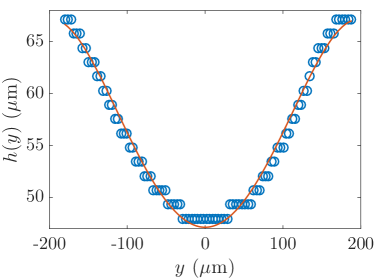
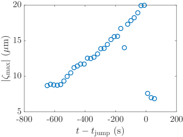
Figure 6: (a) Plot of the local thickness $h(y)$ of the channel from the photograph (iii) in figure 4b as a function of the spanwise coordinate $y$; the staircase-like rendering of the data points is due to the limited spatial resolution of the confocal microscope. The curve is a fit by the formula $h(y)=h-|\zeta_{\max}|(1-4y^{2}/w_{\mathrm{out}}^{2})$ with $|\zeta_{\max}|$ a free fitting parameter, here equal to 20.0 $\mu$m. (b) Plot of $|\zeta_{\max}|$ as a function of time.

3.5 Influence of surface tension

The experiments were also carried out using ethanol as the liquid. Similar jumps were observed, characterised by a length $L_{\mathrm{jump}\>(\mathrm{ethanol})}$. When comparing $L_{\mathrm{jump}\>(\mathrm{ethanol})}$ with the jump length $L_{\mathrm{jump}\>(\mathrm{water})}$ obtained with water in the same geometry, we observe the jump is systematically shorter with ethanol than with water, as represented in figure 7a. Experimental data are well adjusted by the linear relationship $L_{\mathrm{jump}\>(\mathrm{water})}=1.84\>L_{\mathrm{jump}\>(\mathrm{ethanol})}$.

This good linear correlation agrees with our scenario involving a capillary threshold, itself proportional to surface tension. However, the prefactor 1.84 is smaller than the surface tension ratio between water and ethanol, which equals 3.3 (taking 22 mN/m for the surface tension of ethanol). Two main reasons may explain this discrepancy. First, the maximal curvature of the meniscus is larger for ethanol than for water due to better wetting conditions, as shown on the two comparative pictures of figure 7b; hence, the ratio of maximal Laplace pressure at the capillary threshold is smaller than the ratio of surface tension. Second, in our experiments, the surface tension of water might be smaller than that of pure water, due to pollution of the interface by the extraction of the uncrosslinked PDMS chains. Indeed, Hourlier-Fargette et al. (2017) showed that the surface tension of water droplets could drop to $52$ mN/m in presence of such a pollution.

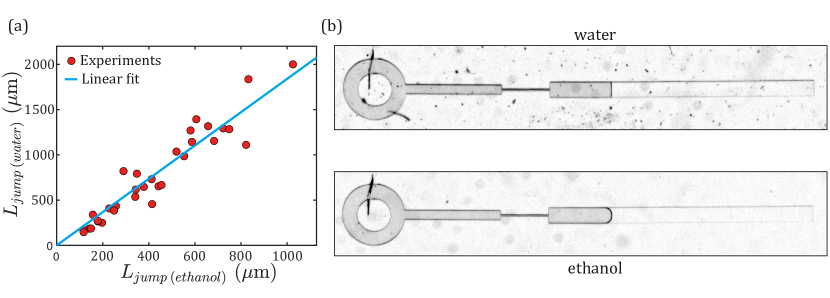
Figure 7: (a) Plot of the length of the jump obtained with water $L_{\mathrm{jump}\>(\mathrm{water})}$ as a function of the length of the jump obtained with ethanol $L_{\mathrm{jump}\>(\mathrm{ethanol})}$ in channels with various geometrical parameters. The straight line corresponds to the best linear fit $L_{\mathrm{jump}\>(\mathrm{water})}=1.84\>L_{\mathrm{jump}\>(\mathrm{ethanol})}$. (b) Two photographs of the air embolism present in the exit channel ($w_{\mathrm{out}}=330$ $\mu$m, $h=53$ $\mu$m, $H=90$ $\mu$m), for both water (top) and ethanol (bottom). The interface curvature between air (at the left) and liquid (at the right) is markedly larger for ethanol than for water, due to a better wettability.

3.6 Volume conservation during the jump

The characteristic time scale of the jump, varying between 0.1 and 2 s depending on the experiments is systematically much smaller than the characteristic time scale of pervaporation $\tau_{\mathrm{perv}}=w_{\mathrm{out}}/|\dot{L}|$ (with $|\dot{L}|$ the interface speed just after the jump), which is itself of order $10^{3}$ to $10^{4}$ s. We can thus consider that the volume of liquid is conserved during the jump, which implies: $S_{\min}L_{\mathrm{out}}=S_{\mathrm{rem}}(L_{\mathrm{out}}-L_{\mathrm{jump}})$, with $S_{\min}$ the cross-sectional area just before the jump. Hence:

$$\frac{L_{\mathrm{jump}}}{L_{\mathrm{out}}}=\frac{\Delta S}{S_{\mathrm{rem}}},$$ (6)

where $\Delta S=S_{\mathrm{rem}}-S_{\min}$. For a few experiments, we compared the confocal measurements of relative deformation of the channel before and after the jump $\Delta S/S_{\mathrm{rem}}$ with the relative amplitude of the jump $L_{\mathrm{jump}}/L_{\mathrm{out}}$ measured from macroscopic observations realised with the same channels a few days after the confocal imaging experiments. Figure 8 shows that the data are compatible with this scenario of volume conservation during the jump, within a certain margin of error due to the confocal imaging resolution and the relative reproducibility of $L_{\mathrm{jump}}$ discussed earlier.

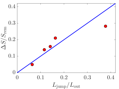
Figure 8: Plot of the relative deformation $\Delta S/S_{\mathrm{rem}}$ observed by confocal imaging, compared to the relative amplitude of the jump $L_{\mathrm{jump}}/L_{\mathrm{out}}$ measured in a second round of experiments with macroscopic observations (red circles). The blue line represents the conservation of water volume during the jump (equation 6).

4 Effect of geometrical parameters on jump length and arrest time

The results shown in section 3 point with good confidence towards the following scenario. The meniscus gets pinned at the constriction corners for a certain time. During this arrest phase, the ongoing drying induces a decrease of the channel cross-section, hence a decrease of the water pressure, and bending of the upper wall. Due to Laplace pressure, this increases the in-plane curvature of the meniscus until a capillary threshold, where a sudden relaxation occurs: the cross-section recovers quickly its equilibrium value, and the meniscus jumps quickly forwards. In this new section, we reinforce the validity of the depicted mechanism by evidencing the influence of the geometrical parameters of the channel (length $L_{\mathrm{out}}$, width $w_{\mathrm{out}}$, membrane thickness $\delta$ and constriction width) on the length of the jump $L_{\mathrm{jump}}$ (sections 4.1, 4.2 and 4.3) and the time of residence in the constriction $t_{\mathrm{res}}$ (section 4.4).

4.1 The jump length $L_{\mathrm{jump}}$ is proportional to the channel length $L_{\mathrm{out}}$

We first report measurements of the jump length as a function of the length the exit channel, for various experiments, in figure 9. It confirms the water volume conservation during the jump (section 3.6), namely that the jump length is simply proportional to the length of the exit channel with an excellent correlation. Moreover, figure 9a shows that, at given exit channel width and channel height, the coefficient of proportionality decreases at increasing upper wall thickness. This proportionality also holds in much longer exit channels (inset of figure 9b).

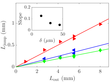
Figure 9: (a) Plot of the jump length $L_{\mathrm{jump}}$ as a function of the length of the exit channel $L_{\mathrm{out}}$, at fixed values of the exit channel width $w_{\mathrm{out}}=300~{}\mu$m and channel height $h=65~{}\mu$m, and for three values of the upper wall thickness: $\delta=15$ ($\blacktriangleright$), 30 ($\blacktriangleleft$) and 45 $\mu$m ($\blacklozenge$). Straight lines are the best linear fits of the three series of data, and the best fitting slope is plotted as a function of $\delta$ in the inset. (b) Plot of the jump length $L_{\mathrm{jump}}$ as a function of the length of the exit channel $L_{\mathrm{out}}$ in channels of width $w_{\mathrm{out}}=300~{}\mu$m, for couples of values of $(h,H)$ equal (in $\mu$m) to: 53, 90 ($\square$); 44, 78 ($\circ$); 53, 79 ($\triangleright$); 65, 89 ($\triangleleft$); 44, 64 ($\times$); 100, 154 ($+$); 53, 85 ($*$); 53, 105 ($\lozenge$). Inset: Plot of the jump length $L_{\mathrm{jump}}$ as a function of the length of the exit channel $L_{\mathrm{out}}$ in long channels of width $w_{\mathrm{out}}=350~{}\mu$m, for $h=67~{}\mu$m and $H=111~{}\mu$m.

The proportionality between the jump length and the length of the exit channel has been interpreted in section 3.6. To make the discussion more complete, it is worth noticing that the quantity $\Delta S$ appearing in (6) depends on the channel compliance and the capillary threshold. Neither of these two quantities depend on $L_{\mathrm{out}}$: the compliance depends on $w_{\mathrm{out}}$, $h$ and $H$, while the capillary threshold depends on $h$ and $w_{\mathrm{p}}$. This further explains the proportionality between the jump length and the length of the exit channel.

4.2 Effect of the channel compliance on the jump length

In order to quantify the effect of the channel compliance, we measured the jump length as a function of the width and the height of the channel and of the upper wall thickness, for various experiments where the length of the exit channel is fixed. We show the influence of the channel width $w_{\mathrm{out}}$ in figure 10a, and that of the upper wall thickness in figure 10b. Figure 10a shows that for each value of $(h,H)$, the jump length increases at increasing channel width, with a convex trend. Figure 10b shows that at given channel width and height, the jump length decreases at increasing upper wall thickness.

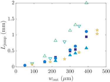
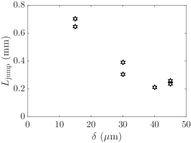
Figure 10: (a) Plot of the jump length $L_{\mathrm{jump}}$ as a function of the width of the exit channel $w_{\mathrm{out}}$ in channels of length $L_{\mathrm{out}}=5.5$ mm, for a fixed channel height $h=53~{}\mu$m and PDMS thickness $H=85$ ($\blacksquare$), 90 ($\bullet$) and 105 $\mu$m ($\blacktriangle$), and a fixed upper wall thickness $\delta=34.5\pm 1~{}\mu$m and channel height $h=35$ ($\triangledown$), 44 ($\triangle$), 53 ($\bullet$) and 60 $\mu$m (pentagram symbols). (b) Plot of the jump length $L_{\mathrm{jump}}$ as a function of the upper wall thickness $\delta$, at fixed values of the length of the exit channel $L_{\mathrm{out}}=5.5~{}$mm, width of the exit channel width $w_{\mathrm{out}}=300~{}\mu$m, and channel height $h=65~{}\mu$m.

The dependence of the jump length on the channel width and upper wall thickness may be discussed in relation with the thin beam approach which was used in section 3 to describe the deflection of the upper wall. From (5) and (6), it is immediate to compute $\Delta S$:

$$\Delta S=\int_{-w_{\mathrm{out}}/2}^{w_{\mathrm{out}}/2}\zeta\,\mathrm{d}y=\frac{w_{\mathrm{out}}^{5}\Delta P}{720B},$$

whence, from (6), the prediction:

$$\frac{L_{\mathrm{jump}}}{L_{\mathrm{out}}}\simeq\frac{w_{\mathrm{out}}^{4}}{60\delta^{3}h}\frac{(1-\nu^{2})\Delta P}{E},$$ (7)

neglecting the difference between $S_{0}$ and $S_{\mathrm{rem}}$ (see the mention to remanent pressure in section 3.3). Hence, the jump length is predicted to be an increasing function of the channel width and a decreasing function of the upper wall thickness, in qualitative agreement with figure 10. The relation (7) also shows that the ratio $L_{\mathrm{jump}}/L_{\mathrm{out}}$ should be proportional to the product of the geometrical dimensionless parameter $w_{\mathrm{out}}^{4}/(60E\delta^{3}h)$, which quantifies the ability of the channel to deform under a given load, and of $(1-\nu^{2})\Delta P/E$. The latter quantity was shown to equal $10^{-3}$ in section 3.4. Since the constriction width $w_{\mathrm{p}}$ remains fixed for this data set, we expect the capillary threshold setting the pressure difference $\Delta P$ not to vary much between all those experiments. Hence, we plot in figure 11 the ratio $L_{\mathrm{jump}}/L_{\mathrm{out}}$ as a function of $w_{\mathrm{out}}^{4}/(60E\delta^{3}h)$, with the straight line of slope $10^{-3}$, gathering all data from figures 9 and 10. It shows that (7) gives the good trend and the good order of magnitude for the jump length as a function of parameters setting the channel compliance, but with a large dispersion. We can evoke several reasons for the limited rescaling of the data: (i) the ratio $\delta/w_{\mathrm{out}}$ is not much larger than one, hence the thin beam theory is only approximate in our experimental conditions. (ii) The clamped end conditions are also approximate, because the bulk of PDMS to which the upper wall is attached is of course not infinitely rigid and may deform. (iii) The capillary threshold may also vary, because it is sensitive to the details of geometry of the constriction exit. Indeed, because of the limited precision of the microfabrication process, the exit corners are not sharp but blunt, with a radius of curvature which may differ between different channels.

It is worth mentioning that our discussion actually concerns the hydraulic capacitance of the channel, a concept used frequently in hydraulics of plants (Brodribb et al., 2005) and in microfluidics (Bruus, 2008). The capacitance links the incoming flux of fluid $Q_{f}$ to the variation of pressure with $Q_{f}=C_{h}\mathrm{d}\Delta P/\mathrm{d}t$. Here the capacitance is due to elastic response of the channel volume, and from (7) we derive (introducing $V_{\mathrm{channel}}=hw_{\mathrm{out}}L_{\mathrm{out}}$ the volume of the channel):

$$C_{h}=\frac{\mathrm{d}V_{\mathrm{channel}}}{\mathrm{d}\Delta P}=\frac{L_{\mathrm{out}}w_{\mathrm{out}}^{5}}{60\delta^{3}}\frac{1-\nu^{2}}{E},$$

a quantity useful to characterise the change of channel volume when pressure varies.

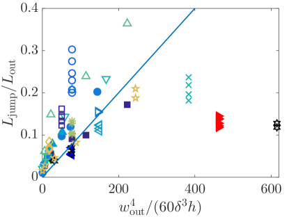
Figure 11: Plot of the ratio $L_{\mathrm{jump}}/L_{\mathrm{out}}$ as a function of $w_{\mathrm{out}}^{4}/(60E\delta^{3}h)$. The straight line is the linear law of slope $10^{-3}$. Different symbols correspond to the various experiments shown in figures 9 and 10.

4.3 Influence of the constriction width $w_{\mathrm{p}}$.

Using channels of various constriction widths $w_{\mathrm{p}}$, we now discuss the influence of the minimal radius of curvature of the interface past the constriction. The mechanism described earlier accounts for a deformation of the channel induced by the Laplace depression in the liquid, itself generated by the strong curvature of the interface in the constriction. It is thereby expected that the jump would be larger for stronger curvature, i.e. for smaller $w_{\mathrm{p}}$. Figure 12 shows three different set of measurements, for three different channel widths $w_{\mathrm{out}}$. It shows that the length of the jump $L_{\mathrm{jump}}$ systematically decreases as the width of the constriction increases, in agreement with the physical mechanism proposed in last section. Although the minimal radius of curvature of the interface is not exactly $w_{\mathrm{p}}/2$ due to the finite angle of the constriction exit (figure 3), data are compatible with inverse power laws (solid lines in figure 12) deriving from (7) with $\Delta P\approx-\gamma/w_{\mathrm{p}}$.

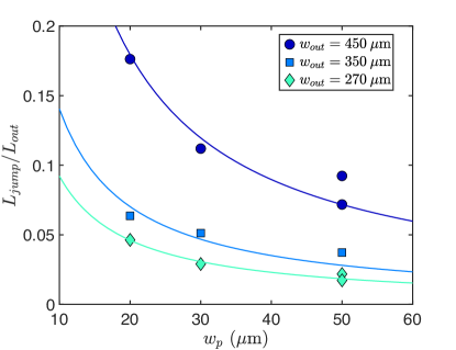
Figure 12: Plot of the ratio $L_{\mathrm{jump}}/L_{\mathrm{out}}$ as a function of the constriction width $w_{\mathrm{p}}$ for three different channel widths $w_{\mathrm{out}}$ (270, 350 and 450 $\mu$m), with $h=67\>\mu$m, $H=95\>\mu$m and $L_{\mathrm{out}}=11$ or $22$ mm. The straight lines correspond to the best inverse fits: $L_{\mathrm{jump}}/L_{\mathrm{out}}=a\cdot w_{\mathrm{p}}^{-1}$, with $a$ a fit parameter.

4.4 Residence time within the constriction $t_{\mathrm{res}}$

Another experimental quantity of interest is the total residence time of the meniscus inside the constriction $t_{\mathrm{res}}$ (shown in figure 2b), which is the counterpart of the time of retention of an air embolism in a tree before propagation in the neighbouring vessel. During this time, the volume of water which leaves the channel by pervaporation is the sum of the volume $hw_{\mathrm{p}}L_{\mathrm{p}}$ of the constriction and of the volume $L_{\mathrm{out}}\Delta S=L_{\mathrm{jump}}S_{\mathrm{rem}}$. The latter contribution comes from our interpretation of the jump length in terms of water conservation leading to the relation (6). Hence, the residence time inside the constriction should equal $t^{*}=(L_{\mathrm{jump}}S_{\mathrm{rem}}+hw_{\mathrm{p}}L_{\mathrm{p}})/Q$, with $Q$ the water flux leaving the channel. For simplicity, we neglect the flux from the water-filled part of the constriction. Therefore, according to the predictions of Dollet et al. (2019) recalled in section 3.1, the water flux equals $Q=q_{\ell}L_{\mathrm{out}}+Q_{g}$, with $q_{\ell}$ the diffusion flux per unit length along the exit channel, and $Q_{g}$ the evaporation flux at the meniscus. We thus get the following prediction:

$$t^{*}=\frac{L_{\mathrm{jump}}S_{\mathrm{rem}}+hw_{\mathrm{p}}L_{\mathrm{p}}}{q_{\ell}L_{\mathrm{out}}+Q_{g}},$$ (8)

with $q_{\ell}$ given by (2), and where, from (4), $Q_{g}=\sqrt{\alpha D_{a}D_{P}hw_{\mathrm{p}}\tilde{q}_{\ell}(w_{\mathrm{p}})}$. The latter flux $Q_{g}$ depends on the dimensions of the channel upstream the meniscus, whence the dependence on the constriction width $w_{\mathrm{p}}$, and not of the exit channel, in the factor $\tilde{q}_{\ell}$.

In figure 13, we plot the residence time inside the constriction as a function of $t^{*}$ calculated using (8), where $D_{P}$ is adjusted so that the condition $t_{\mathrm{res}}=t^{*}$ is best fulfilled. We thus find $D_{P}=5.5\times 10^{-10}$ m²/s. With this fitting value, figure 13 shows indeed a good correspondence between the two times $t_{\mathrm{res}}$ and $t^{*}$. Furthermore, the order of magnitude of the aforementioned value of $D_{P}$ agrees with the value $10^{-9}$ m²/s reported in the literature (Watson & Baron, 1996). Notice that none of the physicochemical parameters $D_{P}$, $\bar{c}_{P}^{\mathrm{sat}}$ and $\alpha$ encountered in the expressions (3) and (4) of the fluxes is known with great precision. Hence, the fact that $t_{\mathrm{res}}$ and $t^{*}$ are found to be equal with reasonable values of these physicochemical parameters tends to confirm our interpretation of the residence time as the time required to pervaporate the water until the capillary threshold is reached.

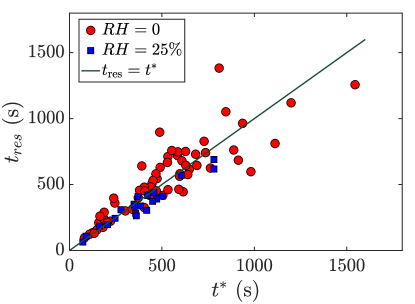
Figure 13: Plot of the residence time of the meniscus inside the constriction $t_{\mathrm{res}}$ as a function of the time $t^{*}$ evaluated from Equation (8) (taking $S_{\mathrm{rem}}=hw_{\mathrm{out}}$), the value $D_{P}=5.5\times 10^{-10}$ m²/s has been taken for the diffusivity of PDMS in water appearing in (2) and (4). Data correspond to different relative humidity: $RH=0\>\%$ (red circles) and $RH=25\>\%$ (blue squares). The straight line corresponds to the equality $t_{\mathrm{res}}=t^{*}$.

5 Relaxation dynamics following the jump

5.1 Description of the dynamics

We also studied the dynamics of the meniscus during the jump, by repeating the reference experiment studied in details in section 3, using a high-speed camera. We supply as Supplementary Material a movie showing the jump and the subsequent relaxation. The water length is plotted as a function of time in figure 14, and an estimation of the instantaneous velocity of the meniscus $|\dot{L}|$ during the fastest phase is plotted as an inset of figure 14. This figure shows that the acceleration at the beginning of the jump phase is larger than the deceleration at the end of this phase. The maximal velocity is 5 mm/s, which is three orders of magnitude larger than the typical speeds of the meniscus in the entrance channel and in the exit channel after the jump (figure 2a). This experiment also confirms the good repeatibility of the jump length.

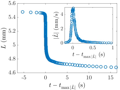
Figure 14: Plot of the water length $L$ as a function of time $t-t_{\max|\dot{L}|}$ in a channel of geometrical parameters $L_{\mathrm{out}}=5.5$ mm, $L_{\mathrm{p}}=1$ mm, $w_{\mathrm{out}}=390~{}\mu$m, $w_{\mathrm{p}}=30~{}\mu$m, $h=65~{}\mu$m and $H=95~{}\mu$m. Inset: plot of the corresponding meniscus velocity $|\dot{L}|$ as a function of time in the fastest phase. The time $t_{\max|\dot{L}|}$ is the instant where the velocity reaches its maximal value.

5.2 Physical discussion

First, it is important to note that the dynamics of the jump (characteristic time scale smaller than $1$ s) is much faster than the pervaporation dynamics (characteristic time scale of about $1000$ s). This confirms that we can neglect the mass loss by pervaporation in the analysis, and consider a constant water volume in the channel throughout the process of the jump.

It is interesting to compare the relaxation dynamics observed in figure 14 to the recent theoretical work by Martínez-Calvo et al. (2020), who studied start-up flows in shallow deformable channels by imposing an initial jump in pressure or in flow rate, and predicted the subsequent dynamics. The corresponding transient flow followed unsteady lubrication theory, with negligible liquid inertia, and the upper wall was modelled by a thin plate under pure bending with clamped end conditions. Our experimental conditions are suited for the comparison. First, we proved that the channel upper wall behaves indeed as a thin plate bent by the pressure difference between the liquid and the outer atmosphere (figure 6). Second, our channel geometry reasonably fulfills the conditions $h\ll w_{\mathrm{out}}\ll L_{\mathrm{out}}$ assumed by Martínez-Calvo et al. (2020). Third, liquid inertia is indeed negligible, as can be checked by evaluating the dimensionless parameter $\varepsilon\mathrm{Re}=\rho h^{4}p_{c}/(12\eta^{2}L_{\mathrm{out}}^{2})$, where $p_{c}$ is the initial pressure jump. We have shown in section 3 that $p_{c}\approx\gamma/w_{\mathrm{p}}=2$ kPa, which leads to the following numerical estimate: $\varepsilon\mathrm{Re}=10^{-1}$, showing that inertia remains a secondary correction and that lubrication theory holds in good approximation. Fourth, the inertia of the top wall can be safely neglected; Martínez-Calvo et al. (2020) showed that the corresponding condition is that the dimensionless parameter defined by $\tilde{\gamma}=3600\rho_{s}\delta h^{6}B/(\eta^{2}L_{\mathrm{out}}^{2}w_{\mathrm{out}}^{4})$, where $\rho_{s}=1.0\times 10^{3}$ kg/m³ is the density of the solid, must be much smaller than 1. Numerical estimation with our parameters leads to $\tilde{\gamma}=7\times 10^{-8}$.

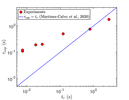
Figure 15: Plot of the characteristic jump time $\tau_{\mathrm{exp}}$ measured experimentally as a function of the elasto-viscous characteristic time $t_{r}$ derived by Martínez-Calvo et al. (2020) (Equation 9). $\tau_{\mathrm{exp}}$ is obtained by an exponential fit of the $L(t)$ plots. Experiments were realized with the following combination of geometric parameters [$h$; $H$; $w_{\mathrm{out}}$; $L_{\mathrm{out}}$; $w_{\mathrm{p}}$] (in $\mathrm{\mu}$m) ordered by increasing value of the measured $\tau_{\mathrm{exp}}$: [11; 56; 100; 8000; 5], [60; 96; 450; 5500; 30], [67; 111; 450; 11000; 20], [67; 111; 450; 22600; 30], [67; 111; 350; 94400; 30], and [67; 111; 350; 182000; 30].

Within such hypotheses, in the model of Martínez-Calvo et al. (2020), the pressure in the channel relaxes following a nonlinear diffusion dynamics, the nonlinearity coming from the dependence of the hydrodynamic resistance on the channel cross-section. In our study, by virtue of the kinematic boundary condition and of the lubrication equations, the meniscus velocity is proportional to the pressure gradient of the liquid in contact. Hence, the temporal dynamics of the meniscus velocity can be compared to that of the pressure in the model of Martínez-Calvo et al. (2020). In this comparison, the key quantity to estimate is the relaxation time of the diffusion dynamics. After a self-similar short-time regime, the long-time regime is an exponential relaxation with a characteristic time:

$$t_{r}=\frac{\eta w_{\mathrm{out}}^{4}L_{\mathrm{out}}^{2}}{60h^{3}B},$$ (9)

see equation (4.5d) in Martínez-Calvo et al. (2020). The numerical evaluation of this characteristic time is $t_{r}=7$ ms, which is way too short to capture the relaxation dynamics shown in our experiments, which is of the order of $\tau_{\mathrm{exp}}\simeq 0.2$ s (figure 14). However, experiments carried out in extremely long channels ($L_{\mathrm{out}}>10$ cm), and leading to remarkably long jumps ($L_{\mathrm{jump}}>1$ cm), exhibit characteristic times $\tau_{\mathrm{exp}}$ comparable to $t_{r}$ (see figure 15). Note that these experimental characteristic times $\tau_{\mathrm{exp}}$ were obtaining after fitting the jump portion of the $L(t)$ curve by a common exponential function $L(t)=L_{\mathrm{out}}-b_{1}[1-\mathrm{e}^{-\left(t-t_{\mathrm{jump}}\right)/\tau_{\mathrm{exp}}}]-b_{2}t$. Here $t_{\mathrm{jump}}$ is the time of the jump, and $b_{1}$ and $b_{2}$ are fitting parameters respectively representing the amplitude of the jump and the pervaporation speed just after the jump.

This puzzling discrepancy between $\tau_{\mathrm{exp}}$ and $t_{r}$ for the fastest jumps suggests that other physical ingredients are at play in our experiments. Contact line friction is one possible such ingredient, but we have checked (see Appendix A) that it is only a correction to the model of Martínez-Calvo et al. (2020) and unable to explain our experimental dynamics.

Other sources of friction in our system originate from the air flow through the constriction and internal friction within PDMS.

The friction of air in the narrow constriction is described using the concept of hydraulic resistance $R_{h}$, linking the difference in pressure to the flow rate of air with $\Delta P=R_{h}Q_{f}$. Since the constriction has a rectangular tall cross-section, we have $R_{h}\simeq{12\eta_{\mathrm{air}}L_{\mathrm{p}}}/{[hw_{\mathrm{p}}^{3}(1-0.630w_{\mathrm{p}}/h)]}$ when $w_{\mathrm{p}}<h$, using the viscosity of air $\eta_{\mathrm{air}}=1.6\times 10^{-5}$ m${}^{2}\cdot\mathrm{s}^{-1}$ (Bruus, 2008). From the hydraulic capacitance $C_{h}$ defined earlier in section 4.2, we predict the relaxation time of the flexible cavity, when friction is dominated by air, to be $\tau=R_{h}C_{h}$. A numerical application provides a value of 2 ms, also way too short.

Concerning internal friction inside the PDMS wall, we can elaborate using results from Placet & Delobelle (2015) showing that the complex elastic modulus for harmonic vibrations, $E^{*}=E^{\prime}+iE^{\prime\prime}$, presents a loss modulus $E^{\prime\prime}$ that is much smaller than the elastic modulus $E^{\prime}$, with a ratio $E^{\prime\prime}/E^{\prime}<0.2$ for frequencies smaller than 100 Hz, as is the case here. According to Landau & Lifshitz (1986), a clamped beam of length $w_{\mathrm{out}}$ and thickness $\delta$ should oscillate at a complex frequency $\omega^{*}=\omega^{\prime}+i\omega^{\prime\prime}=\frac{22.4}{w_{\mathrm{out}}^{2}}\sqrt{\frac{E^{*}\delta^{2}}{12\rho_{\mathrm{PDMS}}}}$, where $\rho_{\mathrm{PDMS}}$ is the density of the solid. A small loss modulus thus means a natural frequency $\omega^{\prime}$ much smaller than attenuation $\omega^{\prime\prime}$: the relaxation of the beam should produce noticeable underdamped oscillations. Here we clearly observe an overdamped relaxation. As a conclusion, internal solid friction does not seem high enough to account for the relaxation time.

6 Summary and outlook

In this study, we have proposed a novel design for biomimetic plant leaves containing constrictions and have shown that they were replicating the role of biological pits in that they enable to recover a strongly intermittent propagation of air embolism. A combination of macroscopic experiments and confocal imaging enabled us to prove that the intermittency is due to a coupling between the compliance of the channel and the capillary pressure at the interface, itself strongly dependent on the constriction geometry.

For future studies, we seek to use this combination of a compliant microchannel and a constriction as a building block for a more complex architecture of biomimetic leaves enabling to reproduce more closely the universal dynamics reported by Brodribb et al. (2016a, b) across various species of plants.

A step further towards more realist biomimetic chips would also consist in replacing PDMS by more hygrophilic materials such as hydrogels or cellulose-based porous materials. Recent studies showed for both wood (Penvern et al., 2020) and cellulose-based fabrics (Ma et al., 2022) that the higher water solubility of these materials leads to dynamics characterized by a most significant role played by bound water.

We anticipate that our results will have significance for a broader audience, in particular in pumpless microfluidic chips (Choi et al., 2017) as well as in chemical engineering where pervaporation is largely employed (Bacchin, Leng & Salmon, 2022). The coupling between the compliance of the channel and the strongly variable pressure induced by the constrictions offer a unique way to passively generate controlled non-linear dynamics.

Appendix A Effect of contact line friction on the relaxation following the jump

In this Appendix, we refine the analysis of Martínez-Calvo et al. (2020) by accounting for the presence of contact line friction at the meniscus. Indeed, such an ingredient is present as soon as contact lines are moving (Snoeijer & Andreotti, 2013), and it significantly affects dynamical processes such as wetting or dewetting dynamics, drop sliding (Winkels et al., 2011) or the damping of sloshing (Dollet, Lorenceau & Gallaire, 2020), to cite but a few examples.

Within the assumptions discussed in section 5.2, Martínez-Calvo et al. (2020) showed that the pressure field in the start-up flow in a shallow deformable channel obeys a nonlinear diffusion equation. The nonlinearity originates from the cross-section-dependent hydrodynamic resistance. For the sake of simplicity, and since our experiments exhibit only moderate cross-section variations (see the snapshots of figure 4b), we neglect this nonlinear effect and the associated channel deformation in this Appendix. The pressure field then obeys the equation:

$$\frac{\partial p}{\partial t}=D\frac{\partial^{2}p}{\partial x^{2}},$$ (10)

with an effective diffusion coefficient given by:

$$D=\frac{60h^{3}B}{\eta w_{\mathrm{out}}^{4}},$$

and an initial condition:

$$p=-p_{c},$$ (11)

where $p_{c}$ is the capillary threshold, i.e. the maximal Laplace pressure reached at the air/liquid interface. The boundary condition at the closed end of the channel $x=L_{\mathrm{out}}$ is:

$$\frac{\partial p}{\partial x}=0.$$ (12)

Martínez-Calvo et al. (2020) considered a sudden release of the pressure from time $t=0$, and at $x=0$. This does not apply in our experiments, for the following reasons. First, the meniscus constitutes a moving boundary, hence the boundary condition should be applied at the time-varying location of the meniscus; we neglect this effect, since the jump length remains generally one order of magnitude shorter than the exit channel length. Second, the pressure release is not instantaneous, and it takes some time for the meniscus to equilibrate once the capillary threshold is passed. Contact line friction is one possible reason for such a delay, which we now consider.

During the post-jump relaxation, the contact angle at the meniscus is a receding contact angle $\theta_{r}$, which obeys Cox–Voinov law (see e.g. Snoeijer & Andreotti (2013)):

$$\theta_{r}^{3}=\theta_{0r}^{3}-\frac{9A\eta|\dot{L}|}{\gamma},$$

where $\theta_{0r}$ is the equilibrium contact angle and $A$ the logarithm of the ratio of a macroscopic cut-off length and a microscopic one, which can be taken with reasonable precision as $A\approx 10$ (the precise value of $A$ will not matter in the subsequent discussion). This velocity-dependent contact angle induces a modulation of Laplace pressure. In principle, we should account for two contact angles at the glass and PDMS interfaces. We neglect this difficulty, as well as the influence of the side walls $y=\pm w_{\mathrm{out}}/2$, and we use the boundary condition:

$$p=-\frac{\gamma}{h}\cos\theta_{r}=-p_{\mathrm{rem}}-\frac{\gamma}{h}(\cos\theta_{r}-\cos\theta_{r0}),$$

where the remanent Laplace pressure $p_{\mathrm{rem}}$ discussed at the end of section 3.3 has been introduced, and where $\theta_{r}$ may be considered as an effective contact angle. In our range of velocities, $|\theta_{r}-\theta_{r0}|\ll 1$, hence we can linearise the boundary condition to obtain:

$$p\simeq-p_{\mathrm{rem}}-\frac{3A\eta\sin\theta_{r0}}{h\theta_{r0}^{3}}|\dot{L}|.$$

Finally, using Poiseuille law $|\dot{L}|=-(h^{2}/12\eta)\partial p/\partial x$, we can write the boundary condition as a mixed boundary condition:

$$p+p_{\mathrm{rem}}=\frac{Ah\sin\theta_{r0}}{4\theta_{r0}^{3}}\frac{\partial p}{\partial x}.$$ (13)

The solution of the diffusion equation (10) with initial condition (11) and boundary conditions (12) and (13) can be found e.g. in section 4.3.6 of Crank (1975). It writes:

$$\frac{p+p_{c}}{p_{c}-p_{\mathrm{rem}}}=1-\sum_{n=1}^{\infty}\frac{2\lambda\cos[\beta_{n}(1-x/L_{\mathrm{out}})]\exp(-\beta_{n}^{2}Dt/L_{\mathrm{out}}^{2})}{(\beta_{n}^{2}+\lambda^{2}+\lambda)\cos\beta_{n}},$$ (14)

where the coefficients $\beta_{n}$ are the positive roots of $\beta\tan\beta=\lambda$, and where $\lambda=4\theta_{r0}^{3}L_{\mathrm{out}}/(Ah\sin\theta_{r0})$. In the current context, this dimensionless parameter compares bulk viscous dissipation to contact line friction. To estimate its numerical value, we take as an effective contact angle $\theta_{r0}=60^{\circ}$, a rough estimate from the snapshots of the meniscus; we then get $\lambda=45$, which suggests that contact line friction remains secondary in the relaxation process. To confirm this fact, we may compute the relaxation time $\tau_{r}$ given by the slowest decaying exponential in (14): $\tau_{r}=L_{\mathrm{out}}^{2}/\beta_{1}^{2}D=t_{r}/\beta_{1}^{2}$, where $t_{r}$ is given by (9). Numerical resolution yields $\beta_{1}=1.54$, whence the estimate $\tau_{r}=3$ ms, way shorter than the experimental relaxation time.

References

- Bacchin et al. (2022) Bacchin, P., Leng, J. & Salmon, J. B. 2022 Microfluidic evaporation, pervaporation, and osmosis: From passive pumping to solute concentration. Chem. Rev. 122, 6938–6985.
- Brodribb et al. (2016a) Brodribb, T. J., Bienaimé, D. & Marmottant, P. 2016a Revealing catastrophic failure of leaf networks under stress. Proc. Natl. Acad. Sci. 113, 4865–4869.
- Brodribb et al. (2005) Brodribb, T. J., Holbrook, N. M., Zwieniecki, M. A. & Palma, B. 2005 Leaf hydraulic capacity in ferns, conifers and angiosperms: impacts on photosynthetic maxima. New Phytol. 165, 839–846.
- Brodribb et al. (2020) Brodribb, T. J., Powers, J., Cochard, H. & Choat, B. 2020 Hanging by a thread? Forests and drought. Science 368, 261–266.
- Brodribb et al. (2016b) Brodribb, T. J., Skelton, R. P., McAdam, S. A. M., Bienaimé, D., Lucani, C. J. & Marmottant, P. 2016b Visual quantification of embolism reveals leaf vulnerability to hydraulic failure. New Phytol. 209, 1403–1409.
- Bruning et al. (2019) Bruning, M. A., Costalonga, M., Snoeijer, J. H. & Marín, Á. 2019 Turning drops into bubbles: cavitation by vapor diffusion through elastic networks. Phys. Rev. Lett. 123, 214501.
- Bruus (2008) Bruus, H. 2008 Theoretical Microfluidics. Oxford University Press.
- Chagua Encarnación et al. (2021) Chagua Encarnación, K. N., Marmottant, P. & Dollet, B. 2021 Pervaporation-induced drying in networks of channels of variable width. Microfluid. Nanofluid. 25, 71.
- Choat et al. (2018) Choat, B., Brodribb, T. J., Brodersen, C. R., Duursma, R. A., López, R. & Medlyn, B. E. 2018 Triggers of tree mortality under drought. Nature 558, 531–539.
- Choat et al. (2010) Choat, B., Drayton, W. M., Brodersen, C., Matthews, M. A., Shackel, K. A., Wada, H. & McElrone, A. J. 2010 Measurement of vulnerability to water stress-induced cavitation in grapevine: a comparison of four techniques applied to a long-vesseled species. Plant Cell Environ. 33, 1502–1512.
- Choat et al. (2012) Choat, B., Jansen, S., Brodribb, T., Cochard, H., Delzon, S., Bhaskar, R., Bucci, S. J., Feild, T. S., Gleason, S. M., Hacke, U. G. & et al. 2012 Global convergence in the vulnerability of forests to drought. Nature 491, 752–755.
- Choi et al. (2017) Choi, J., Kang, D., Han, S., Kim, S. B. & Rogers, J. A. 2017 Thin, soft, skin-mounted microfluidic networks with capillary bursting valves for chrono-sampling of sweat. Adv. Healthc. Mater. 6, 1601355.
- Christov et al. (2018) Christov, I. C., Cognet, V., Shidhore, T. & Stone, H. A. 2018 Flow rate–-pressure drop relation for deformable shallow microfluidic channels. J. Fluid Mech. 841, 267–286.
- Cochard et al. (1992) Cochard, H., Cruiziat, P. & Tyree, M. T. 1992 Use of positive pressures to establish vulnerability curves: further support for the air-seeding hypothesis and implications for pressure-volume analysis. Plant Physiol. 100, 205–209.
- Cochard et al. (2015) Cochard, H., Delzon, S. & Badel, E. 2015 X-ray microtomography (micro-ct): a reference technology for high-resolution quantification of xylem embolism in trees. Plant Cell Environ. 38, 201–206.
- Comtet et al. (2017) Comtet, J., Jensen, K. H., Turgeon, R., Stroock, A. D. & Hosoi, A. E. 2017 Passive phloem loading and long-distance transport in a synthetic tree-on-a-chip. Nat. Plants 3, 1–8.
- Crank (1975) Crank, J. 1975 The Mathematics of Diffusion. Oxford University Press.
- Dollet et al. (2021) Dollet, B., Chagua Encarnación, K. N., Gautier, R. & Marmottant, P. 2021 Drying by pervaporation in elementary channel networks. J. Fluid Mech. 906, A6.
- Dollet et al. (2020) Dollet, B., Lorenceau, É. & Gallaire, F. 2020 Transition from exponentially damped to finite-time arrest liquid oscillations induced by contact line hysteresis. Phys. Rev. Lett. 124, 104502.
- Dollet et al. (2019) Dollet, B., Louf, J. F., Alonzo, M., Jensen, K. H. & Marmottant, P. 2019 Drying of channels by evaporation through a permeable medium. J. R. Soc. Interface 16, 20180690.
- Duan et al. (2012) Duan, C., Karnik, R., Lu, M.-C. & Majumdar, A. 2012 Evaporation-induced cavitation in nanofluidic channels. Proc. Nat. Ac. Sci. 109, 3688–3693.
- Ducloué et al. (2017a) Ducloué, L., Hazel, A. L., Pihler-Puzović, D. & Juel, A. 2017a Viscous fingering and dendritic growth under an elastic membrane. J. Fluid Mech. 826, R2.
- Ducloué et al. (2017b) Ducloué, L., Hazel, A. L., Thompson, A. B. & Juel, A. 2017b Reopening modes of a collapsed elasto-rigid channel. J. Fluid Mech. 819, 121–146.
- Fontana et al. (2021) Fontana, J. V., Juel, A., Bergemann, N., Heil, M. & Hazel, A. L. 2021 Modelling finger propagation in elasto-rigid channels. J. Fluid Mech. 916, A27.
- Fukuda et al. (2015) Fukuda, K., Kawaguchi, D., Aihara, T., Ogasa, M. Y., Miki, N. H., Haishi, T. & Umebayashi, T. 2015 Vulnerability to cavitation differs between current-year and older xylem: non-destructive observation with a compact magnetic resonance imaging system of two deciduous diffuse-porous species. Plant Cell Environ. 38, 2508–2518.
- Gervais et al. (2006) Gervais, T., El-Ali, J., Günther, A; & Jensen, K. F. 2006 Flow-induced deformation of shallow microfluidic channels. Lab Chip 6, 500–507.
- Grotberg (1994) Grotberg, J. B. 1994 Pulmonary flow and transport phenomena. Annu. Rev. Fluid Mech. 26, 529–571.
- Grotberg & Jensen (2004) Grotberg, J. B. & Jensen, O. E. 2004 Biofluid mechanics in flexible tubes. Annu. Rev. Fluid Mech. 36, 121–147.
- Géraud et al. (2016) Géraud, B., Jones, S. A., Cantat, I., Dollet, B. & Méheust, Y. 2016 The flow of a foam in a two-dimensional porous medium. Water Resour. Res. 52, 773–790.
- Hardy et al. (2009) Hardy, B. S., Uechi, K., Zhen, J. & Kavehpour, H. P. 2009 The deformation of flexible pdms microchannels under a pressure driven flow. Lab Chip 9, 935–938.
- Harley et al. (2012) Harley, S. J., Glascoe, E. A. & Maxwell, R. S. 2012 Thermodynamic study on dynamic water vapor sorption in sylgard-184. J. Phys. Chem. B 116, 14183–14190.
- Heil & Hazel (2011) Heil, M. & Hazel, A. L. 2011 Fluid-structure interaction in internal physiological flows. Annu. Rev. Fluid Mech. 43, 141–162.
- Heil & Hazel (2016) Heil, M. & Hazel, A. L. 2016 Flow in flexible/collapsible tubes. In Fluid–Structure Interaction in Low-Reynolds-Number Flows (ed. C. Duprat & H. A. Stone), pp. 280–312. Royal Society of Chemistry.
- Heil et al. (2008) Heil, M., Hazel, A. L. & Smith, J. A. 2008 The mechanics of airway closure. Respir. Physiol. Neurobiol. 163, 214–221.
- Holden et al. (2003) Holden, M. A., Kumar, S., Beskok, A. & Cremer, P. S. 2003 Microfluidic diffusion diluter: bulging of pdms microchannels under pressure-driven flow. J. Micromech. Microengin. 13, 412.
- Hölttä et al. (2009) Hölttä, T., Cochard, H., Nikinmaa, E. & Mencuccini, M. 2009 Capacitive effect of cavitation in xylem conduits: results from a dynamic model. Plant Cell Environ. 32, 10–21.
- Hourlier-Fargette et al. (2017) Hourlier-Fargette, A., Antkowiak, A., Chateauminois, A. & Neukirch, S. 2017 Role of uncrosslinked chains in droplet dynamics on silicon elastomers. Soft Matter 13, 3484–3491.
- Jensen et al. (2009) Jensen, K. H., Rio, E., Hansen, R., Clanet, C. & Bohr, T. 2009 Osmotically driven pipe flows and their relation to sugar transport in plants. J. Fluid Mech. 636, 371–396.
- Juel et al. (2018) Juel, A., Pihler-Puzović, D. & Heil, M. 2018 Instabilities in blistering. Annu. Rev. Fluid Mech. 50, 691–714.
- Katifori et al. (2010) Katifori, E., Szöllősi, G. J. & Magnasco, M. O. 2010 Damage and fluctuations induce loops in optimal transport networks. Phys. Rev. Lett. 104, 048704.
- Landau & Lifshitz (1986) Landau, L. D. & Lifshitz, E. M. 1986 Theory of Elasticity, 3rd edn. Elsevier.
- Lenormand & Zarcone (1985) Lenormand, R. & Zarcone, C. 1985 Invasion percolation in an etched network: Measurement of a fractal dimension. Phys. Rev. Lett. 54, 2226–2229.
- Ma et al. (2022) Ma, X., Maillet, B., Brochard, L., Pitois, O., Sidi-Boulenouar, R. & Coussot, P. 2022 Vapor-sorption coupled diffusion in cellulose fiber pile revealed by magnetic resonance imaging. Phys. Rev. Appl. 17, 024048.
- Måløy et al. (1985) Måløy, K. J., Feder, J. & Jøssang, T. 1985 Viscous fingering fractals in porous media. Phys. Rev. Lett. 55, 2688–2691.