Accelerating potential evaluation over unstructured meshes in two dimensions

Zewen Shen$\mbox{}^{\dagger\,\star}$ and Kirill Serkh$\mbox{}^{\ddagger\,\diamond}$

June 16, 2022

$\mbox{}^{\diamond}$ This author’s work was supported in part by the NSERC Discovery Grants RGPIN-2020-06022 and DGECR-2020-00356.

$\mbox{}^{\dagger}$ Dept. of Computer Science, University of Toronto, Toronto, ON M5S 2E4
$\mbox{}^{\ddagger}$ Dept. of Math. and Computer Science, University of Toronto, Toronto, ON M5S 2E4

$\mbox{}^{\star}$ Corresponding author

1 Introduction

Integral equation methods solve partial differential equations (PDEs) by reformulating them as integral equations using the tools of potential theory. The accurate and efficient evaluation of potentials with singular or weakly-singular kernels, over curves, surfaces and volumes, is thus of great importance for the numerical solution of PDEs. However, their numerical evaluation poses several difficulties. Firstly, the potential is often expressed as a convolution of a Green’s function with a density function, and due to the singularity of the Green’s function, special integration techniques must be employed. Secondly, the integration domain of the potential could be complicated, which requires it to either be embedded into a larger regular domain, or to be resolved by adaptive meshing. Finally, the scheme for evaluating the potential must be compatible with fast algorithms (e.g., the fast multipole method (FMM) or the fast Fourier transform (FFT)) for achieving linear or quasi-linear time complexity. We note that, when the integration domain is regular, the difficulties stated above can be easily overcome by exploiting the translational invariance of the free-space Green’s function. More specifically, given a regular domain that is discretized by a rectangular mesh, the dimensionality of the function spaces of near field and self-interactions is finite, and, thus, these interactions can be efficiently tabulated, from which it follows that the box code [9, 3] can be used to compute the potential in linear time with a small constant. However, when the integration domain is irregular, provided that the domain is discretized by an unstructured mesh, the function spaces of near field and self-interactions are non-compact, and, thus, one can no longer easily accelerate the computation by precomputations.

Existing methods for computing the potential over an irregular domain generally fall into two categories. The first one is based on the observation that the volume potential is the solution to an elliptic interface problem, where the irregular domain $\Omega$ is embedded inside a regular box (see, for example, [2], for details). A finite difference method with corrections based on knowledge of the jumps in the solution across $\partial\Omega$ is applied, with the order of accuracy determined by the finite difference scheme used. Additionally, the method is compatible with the FFT when a uniform grid is used to discretize the domain, and, thus, it can achieve a quasi-linear time complexity. We note that, although this approach saves the trouble of meshing an irregular domain, its order of convergence is usually low, and it is not highly compatible with adaptive mesh refinement. Furthermore, the method doesn’t easily generalize to the surface potential case.

The methods belonging to the second category compute the potential directly by quadrature. More specifically, the domain $\Omega$ is discretized into an unstructured mesh, and for each target location $x$, depending on its proximity to the mesh elements, different quadrature schemes are used to compute the integral over each mesh element, which leads to a spectrally accurate evaluation. Moreover, the computation of the far field interactions (i.e., integrals over mesh elements that are far away from $x$) can be accelerated by the FMM, which results in linear total time complexity. We note that research into methods of this type has mostly focused on the surface potential case, despite the fact that the algorithms for computing the surface potential have great similarities with the ones for computing the 2-D volume potential. We refer the readers to [1] for a thorough literature review of methods belonging to these two categories.

Despite the advantages of the direct approach of computing the potential by quadrature (i.e., spectral accuracy and linear time complexity), the actual constants in time complexity are usually large, due to the cost associated with the near field and self-interaction computations, which cannot be efficiently precomputed over an unstructured mesh. In [1], the authors propose a remedy to this issue. Given an irregular domain $\Omega$, they embed a rectangular mesh inside a large regular subdomain of $\Omega$, and fill the rest of the domain with unstructured meshes that conform to the curved boundary. It follows that a large proportion of the evaluations can be accelerated by the box code, while respecting the true geometry of the domain to retain spectral accuracy. However, as the authors of [1] point out, the computation of near field and self-interactions over the unstructured mesh forms the majority of the costs in their algorithm, even when the unstructured mesh elements only make up a small proportion of the total mesh elements. Furthermore, such a remedy is not applicable to surface potential evaluation. Therefore, we regard potential evaluation over unstructured meshes as a problem of great importance in integral equation methods.

In this paper, we propose the following novel and complementary techniques for accelerating the near and self-interaction computations over an unstructured mesh. Below, we briefly describe the techniques.

1. In the classic literature, the near field is typically approximated by a ball or a triangle. We observe that this often leads to an overestimation of the true near field, especially when the order of the quadrature or the error tolerance is high, which leads to substantial unnecessary and expensive near field interaction computations. Thus, we rigorously characterize the geometry of the near field, which allows us to dramatically reduce the number of the required near field interaction computations. Specifically, we show that the near field is approximately equal to the union of several Bernstein ellipses. In addition, this technique provides error control functionality to the far and near field interaction computations. For example, this technique allows for a precise determination of the number of required subdivisions of the element domain when the near field interactions are computed adaptively, which avoids the possibility both of oversampling and of undersampling.

2. Since our analysis shows that the near field can be made arbitrarily small by increasing the order of the far field quadrature rule, we observe that one can efficiently offload the near field interaction computation onto the FMM-based far field interaction computation. This trade leverages the computational efficiency of highly optimized parallel FMM libraries, and reduces the cost of the much more expensive and unstructured near field interaction computation. Furthermore, this offloading technique is one of the few applications we are aware of that requires the use of extremely high-order (say, $50$th order) quadrature rules in high dimensions.

3. When one interpolates the potential, we observe that the most commonly used arrangement of the quadrature nodes and interpolation nodes, where they are both placed over a single mesh, leads to an artificially large near field and self-interaction computation cost. If the quadrature and interpolation nodes are instead placed over two separate meshes that are staggered to one another, the number of interpolation nodes at which the near field and self-interactions are costly to evaluate is reduced dramatically.

We note that the near field geometry analysis for the 1-D layer potential computed by the trapezoidal rule and the Gauss-Legendre rule has been rigorously carried out in [4] and in [17, 18], respectively, and recently, the authors of [19] characterize the near field geometry of the surface potential in $\mathbbm{R}^{3}\setminus S$, where $S$ is the surface over which the potential is generated. The near field geometry analysis for volume potentials has not been carried out previous to this paper. Furthermore, we point out that the near field geometry analysis is much more powerful in high dimensions (i.e., 2-D volumes, 3-D volumes, surfaces), since the intersection of the near field with the domain over which the potential is generated becomes non-negligible in these situations, and thus, the computation of the near field interactions becomes a bottleneck when solving integral equations over these domains. We also note that the idea of increasing the order of the far field quadrature rule to reduce the amount of near field interaction computation appears, for example, in [16, 1]. However, it is presented as a heuristic. In fact, without characterizing the geometry of the near field precisely, such an idea cannot be optimally carried out. As we show in this paper, the near field is approximately equal to the union of several Bernstein ellipses, and when the order of the far field quadrature is high, their area becomes vanishingly small. Thus, a naive estimation of the near field (by a ball [16, 6] or a triangle [1]) is seen to be poor, and a large proportion of the near field interaction computations are unnecessary. In addition to this, when a naive estimation of the near field is used, one has to overestimate the size of the near field to improve the robustness of the algorithm, which further increases the unnecessary cost.

One would generally expect that a reduction in the area of the near field leads to a reduction in the cost of the computation of near field interactions. However, this turns out to be false, in the common case where the target points are chosen to be interpolation nodes over the same triangle mesh as the one that is used for quadrature. The discretization nodes tend to cluster near the edges of the mesh elements, which means that a smaller near field does not necessarily result in a commensurate reduction in the computational cost. With the use of a separate interpolation mesh that is staggered to the quadrature mesh, the reduction in the near field interaction computation cost becomes proportional to the reduction in the area of the near field. The techniques that we present are thus complementary.

In this paper, for simplicity, we only consider the evaluation of the 2-D Newtonian potential over an irregular domain $\Omega$,

$$u(x)=\iint_{\Omega}\frac{1}{2\pi}\log{\lVert x-y\rVert}f(y)\,\mathrm{d}A_{y}.$$ (1)

We note that our techniques can be easily generalized to kernels of other types and, also, with some additional work, to surface and 3-D volume potential evaluations.

Besides the general contributions to potential evaluation problems that we describe above, we make the following contributions that are specific to the 2-D volume potential evaluation problem.

• We describe a robust and extensible framework for evaluating and interpolating 2-D volume potentials over complicated geometries, without the need for extensive precomputation. Our presentation makes minimal use of specialized quadrature rules, although our framework is compatible with their use.

• Although a well-conditioned formula for computing self-interactions has already appeared, for example, in [32, 1], its standard derivation is somewhat overcomplicated and the necessity of the formula is not fully motivated. We instead present a short and elementary derivation of the same formula from the first principles, and explain why it is needed.

• We provide a description of a full and robust pipeline of the geometric algorithms that are required for the volume potential evaluation, e.g., a meshing algorithm, a nearby element query algorithm, etc.

We conduct several numerical experiments to demonstrate the performance of the techniques for accelerating the computation over an unstructured mesh. We also report the overall performance of our volume potential evaluation algorithm.

2 Mathematical preliminaries

2.1 Koornwinder polynomials

The Koornwinder polynomials, denoted by $K_{nm}:\Delta^{1}\to\mathbbm{R}$, are defined by

$$K_{mn}(x,y)=c_{mn}(1-x)^{m}P_{n-m}^{(2m+1,0)}(2x-1)P_{m}\Bigl{(}\frac{2y}{1-x}-1\Bigr{)},\quad m\leq n,$$ (2)

where

$$\Delta^{1}=\{(x,y)\in\mathbbm{R}^{2}:0\leq x\leq 1,0\leq y\leq 1-x\}$$ (3)

is the standard simplex, $P_{k}^{(a,b)}$ is the Jacobi polynomial of degree $k$ with parameters $(a,b)$, $P_{m}$ is the Legendre polynomial of degree $m$, and $c_{mn}$ is the normalization constant such that

$$\int_{\Delta^{1}}{\lvert K_{mn}(x,y)\rvert}^{2}\,\mathrm{d}x\,\mathrm{d}y=1.$$ (4)

It is observed in [20] that the $(N+1)(N+2)/2$ functions

$$\bigl{\{}K_{mn}(x,y):n=0,\dots,N,m=0,\dots,n\bigr{\}}$$ (5)

form an orthogonal basis for $\mathcal{P}_{N}$ on the standard simplex $\Delta^{1}$, where $\mathcal{P}_{N}$ denotes the space of polynomials of order at most $N$ on $\Delta^{1}$. In addition, by orthogonality, we also have that

$$\int_{\Delta^{1}}K_{mn}(x,y)\,\mathrm{d}x\,\mathrm{d}y=0,$$ (6)

for any $m,n\in\mathbbm{N}_{\geq 0}$ with $m+n>0$.

2.2 Quadrature and interpolation over triangles

On a two-dimensional domain, a quadrature rule of length $n$ is optimal if it integrates $3n$ functions (since the total number of degrees of freedom of the rule is $3n$), and we refer to such a rule as a generalized Gaussian quadrature rule. In general, the efficiency of a quadrature rule is defined to be $E=\frac{m}{(d+1)n}$, where $d$ is the dimensionality of the domain, $n$ is the length of the quadrature rule, and $m$ is the dimensionality of the space of functions that can be integrated exactly using that rule (see [28] for details).

Although the construction (or even the existence) of perfect generalized Gaussian quadrature rules over two-dimensional domains remains an open problem, various schemes for generating nearly-perfect ones exist, e.g., [26, 28]. In this section, we describe some quadrature and interpolation schemes for polynomials over a triangle domain.

The Vioreanu-Rokhlin rule, introduced in [26], takes two integers $N$ and $M\geq N$ as inputs, and attempts to generate a quadrature rule of length exactly $\dim\mathcal{P}_{N}$ that integrates all functions in $\mathcal{P}_{M}$ over a given convex domain exactly. The method is based on the observation that elements of the complex spectrum of the multiplication operator restricted to $\mathcal{P}_{N}$, acting on any convex domain, turn out to be excellent quadrature nodes for integrating all functions in $\mathcal{P}_{N}$ over the domain. These nodes are used as an initial guess by the Vioreanu-Rokhlin algorithm and iteratively improved (by solving a nonlinear least-squares problem) to integrate all functions in $\mathcal{P}_{M}$. As a result, the generated rule is generally efficient and of high quality. Additionally, the set of quadrature nodes can also serve as interpolation nodes for approximating functions in $\mathcal{P}_{N}$, since the length of the rule equals $\dim\mathcal{P}_{N}$. To get the interpolation matrix, we invert the matrix that maps the Koornwinder polynomial expansion coefficients to function values at the interpolation nodes. Using the Vioreanu-Rokhlin nodes as the interpolation nodes, the condition number of this interpolation matrix turns out to be small, which guarantees that the interpolation is stable.

In the situation where interpolation is not needed, one can loosen the restriction in the Vioreanu-Rokhlin algorithm that the length of the quadrature rule equals $\dim\mathcal{P}_{N}$ for some $N$, and this can result in a more efficient quadrature algorithm. This fact is used by the Xiao-Gimbutas algorithm [28], which is also based on solving a nonlinear least-squares problem. For example, the Xiao-Gimbutas rule of length 78 integrates $\mathcal{P}_{20}$ exactly, while the Vioreanu-Rokhlin rule needs to have a length equal to $\dim\mathcal{P}_{12}=91$ to accomplish the same job. We tabulate the lengths and orders of some Xiao-Gimbutas rules and Vioreanu-Rokhlin rules in Tables 2 and 3.

2.3 The polar tangential angle

In this section, we describe some concepts in differential geometry that we make use of in the sequel.

Definition 2.1.

Given a unit-speed parametrized curve $\gamma(s)$, we define the polar tangential angle $\psi(s)$ of $\gamma$ with respect to polar coordinates centered at $O$ to be

$$\psi(s)=\angle(\gamma^{\prime}(s),\gamma(s)-O),$$ (7)

where $\gamma$ is parameterized by arc length (see Figure 1). In other words, $\psi(s)$ represents the angle between the tangent line to the curve at $\gamma(s)$ and the ray from $O$ to the point.

Figure 1: The polar tangential angle $\psi(s)$.

Let the polar angle $\theta(s)$ be the angle of the point $\gamma(s)$ in polar coordinates with respect to the origin $O$. The following theorem illustrates how to compute the derivative of the polar angle of a given curve, given its radius and polar tangential angle. The proof of the theorem can be found in Chapter 12 of [27].

Theorem 2.1.

Suppose that $\gamma(s)$ is a unit-speed parametrized curve. Suppose further that $r_{0}(s)$ and $\theta(s)$ are the radius and polar angle, respectively, of $\gamma(s)$ with respect to a given polar coordinate system. Then

$$\theta^{\prime}(s)=\frac{\sin(\psi(s))}{r_{0}(s)},$$ (8)

where $\psi(s)$ is the polar tangential angle of $\gamma$ at $\gamma(s)$.

It turns out that the derivative $\theta^{\prime}(s)$ can be expressed directly in terms of $\gamma(s)$ and $r_{0}(s)$.

Corollary 2.2.

Suppose that $\gamma(s)$ is a unit-speed parametrized curve. Suppose further that $r_{0}(s)$ and $\theta(s)$ are the radius and polar angle, respectively, of $\gamma(s)$ with respect to a given polar coordinate system centered at $O$. Then

$$\theta^{\prime}(s)=\frac{{\lvert(\gamma(s)-O)\times\gamma^{\prime}(s)\rvert}}{r_{0}^{2}(s)}.$$ (9)

Proof. By definition of the cross product, we have that

$${\lvert(\gamma(s)-O)\times\gamma^{\prime}(s)\rvert}=r_{0}(s)\sin(\psi(s)).$$ (10)

By combining (8) and (10), we prove the result. $\blacksquare$

2.4 Approximation of analytic functions by polynomials

In this section, we describe several concepts in approximation theory that we make use of in the sequel.

Definition 2.2.

Given a real number $\rho>1$, the Bernstein ellipse with parameter $\rho$ is defined to be the ellipse

$$\Bigl{\{}(z+z^{-1})/2:z=\rho e^{i\theta},\theta\in[0,2\pi)\Bigr{\}}.$$ (11)

Furthermore, we denote the interior of the Bernstein ellipse by $E_{\rho}$. In a slight abuse of notation, we also refer to $E_{\rho}$ as the Bernstein ellipse, when the meaning is clear.

The proof of the following two theorems can be found in [25].

Theorem 2.3.

Suppose $f$ is a function on $[-1,1]$ for which there exist a sequence of polynomials $q_{0},q_{1},\dots$, where $q_{n}$ is a polynomial of order $n$, satisfying

$${\lVert f-q_{n}\rVert}_{L^{\infty}[-1,1]}\leq C\rho^{-n},$$ (12)

for some integer $n\geq 0$, and some real numbers $\rho>1,C>0$. Then $f$ can be analytically continued to an analytic function in $E_{\rho}$.

Theorem 2.4.

Suppose that an analytic function $f:[-1,1]\to\mathbbm{R}$ is analytically continuable to $E_{\rho}$, for some real number $\rho>1$. Suppose further that ${\lvert f(z)\rvert}$ is bounded inside $E_{\rho}$ by some constant $M$. Then,

$${\lVert f-f_{n}\rVert}_{L^{\infty}[-1,1]}\leq\frac{2M\rho^{-n}}{\rho-1},$$ (13)

for all $n\geq 0$, where $f_{n}$ denotes the $n$th order Chebyshev projection of $f$, by which we mean the infinite expansion of $f$ in terms of Chebyshev polynomials, truncated at the $n$th order (inclusive).

The following corollary is an immediate consequence of Theorem 2.4.

Corollary 2.5.

Suppose that an analytic function $f:[-1,1]\to\mathbbm{R}$ is analytically continuable to $E_{\rho}$, for some real number $\rho>3/2$. Suppose further that ${\lvert f(z)\rvert}$ is bounded inside $E_{\rho}$ by $1/4$. Then,

$${\lVert f-f_{n}\rVert}_{L^{\infty}[-1,1]}\leq\rho^{-n},$$ (14)

for all $n\geq 0$, where $f_{n}$ denotes the $n$th order Chebyshev projection of $f$, by which we mean the infinite expansion of $f$ in terms of Chebyshev polynomials, truncated at the $n$th order (inclusive).

3 Volume potential evaluation over complicated geometries

In this section, we describe a numerical apparatus for computing and interpolating the volume potential

$$u(v)=\iint_{\Omega}\log({\lVert v-y\rVert})f(y)\,\mathrm{d}A_{y},$$ (15)

where the target location $v\in\mathbbm{R}^{2}$, and $\Omega$ is a smooth planar domain. We first discretize $\Omega$ into a triangle mesh (see Appendices A.3, A.4 for details), and reduce the problem to the case where the integration region is either a triangle $\overline{\Delta}$ or a curved element $\widetilde{\Delta}$ (a mesh element with three sides, one of which is curved). Furthermore, we divide each of these two problems into three distinct subproblems: where $v$ is far from the element (i.e., far field interactions), where $v$ is close to the element (i.e., near field interactions), where $v$ lies within the element (i.e., self-interactions). Our goal is to present a simple and robust framework for handling these different types of the interactions. In particular, we minimize the use of special-purpose quadrature rules in our discussion, although it could potentially speed up the algorithm. We note that, however, our framework is compatible with such rules. In addition, we describe an interpolation scheme for the volume potential over a mesh element. In the end, we describe how to couple the algorithms with the fast multipole method (FMM) to evaluate the volume potential generated over $\Omega$ at any given set of target locations, with linear time complexity.

For simplicity, we refer to both standard triangles and curved elements as mesh elements when there is no ambiguity.

3.1 Integration over a mesh element

In this section, we introduce algorithms for generating efficient quadrature rules for integrating smooth functions over an arbitrary mesh element $\Delta$ (either a triangle or a curved element).

Recall that in Section 2.2, we describe how to obtain a nearly-perfect Gaussian quadrature rule for integrating polynomials over the standard simplex

$$\Delta^{1}=\{(x,y)\in\mathbbm{R}:0\leq x\leq 1,0\leq y\leq 1-x\}.$$ (16)

Clearly, provided that an invertible and well-conditioned mapping $\rho:\Delta^{1}\to\Delta$ is given, the generation of a quadrature rule over $\Delta$ is simple, and is described in the following theorem.

Theorem 3.1.

Given the standard simplex $\Delta^{1}$ and a mesh element $\Delta$, suppose that $\{(x_{i},y_{i}),w_{i}\}_{i}$ is a set of quadrature nodes and weights that integrates $\{K_{mn}\}_{m,n}$ exactly over $\Delta^{1}$, and $\rho$ is an invertible and well-conditioned mapping from $\Delta^{1}$ to $\Delta$. Then,

$$\bigl{\{}\rho(x_{i},y_{i}),w_{i}\cdot{\lvert J_{\rho}(x_{i},y_{i})\rvert}\bigr{\}}_{i}$$ (17)

is the set of quadrature nodes and weights that integrates $\{K_{mn}\circ\rho^{-1}\}_{m,n}$ exactly over the mesh element $\Delta$, where $J_{\rho}(x)$ denotes the Jacobian determinant of $\rho$ at $x$.

Proof. The theorem follows directly from a change of variables. $\blacksquare$

Therefore, the problem of evaluating an integral over a mesh element reduces to the computation of an invertible and well-conditioned mapping $\rho$ from $\Delta^{1}$ to $\Delta$. When $\Delta$ is a triangle, there exists an affine transformation from $\Delta^{1}$ to $\Delta$, so the mapping $\rho$ can be constructed easily, and ${\lvert J_{\rho}(x_{i},y_{i})\rvert}=\text{area}(\Delta)/\text{area}(\Delta^{1})$. When $\Delta$ is a curved element, the blending function method [13, 14, 30] provides an elegant solution to the problem, as is mentioned in [1]. Below, we describe the method.

Let $\gamma:[0,L]\to\mathbbm{R}^{2}$ be the unit-speed parametrization of the curved side of a curved element $\widetilde{\Delta}$, and let $O:=(x_{0},y_{0})$ denote the vertex opposite to the curved side. Then for any point $(\xi,\eta)\in\Delta^{1}$, define

$$\rho(\xi,\eta):= \ (1-\xi-\eta)\cdot\gamma(L)+\xi\cdot\gamma(0)+\eta\cdot O$$

$$+ \frac{1-\xi-\eta}{1-\xi}\Bigl{(}\gamma\bigl{(}L(1-\xi)\bigr{)}-(1-\xi)\cdot\gamma(L)-\xi\cdot\gamma(0)\Bigr{)}.$$ (18)

It can be shown that $\rho$ is an invertible and well-conditioned mapping from $\Delta^{1}$ to $\widetilde{\Delta}$, and its Jacobian $J_{\rho}$ can be computed by a straightforward calculation.

Remark 3.1.

When the curved side $\gamma$ is a straight line segment (i.e., the curved element is a triangle), the mapping $\rho$ generated by the blending function method degenerates into an affine mapping, which implies that the discussion in this section can be unified under the blending function method framework. For clarity and computational efficiency purposes, the discussions of the two cases are separated.

Observation 3.2.

In the case where the curved side of a curved element is not well-resolved by the mesh, the Jacobian of the blending function $\rho$ becomes non-smooth, which requires a relatively large number of degrees of freedom to approximate. Thus, when the requirement for high accuracy is rigid, it is important to refine the mesh around the region where the geometry of the boundary is complicated, or use a quadrature rule of order higher than the one for triangle elements.

3.2 Far field interactions

In this section, we introduce far field quadrature rules for computing the volume potential (15) when the integration domain $\Omega$ is a mesh element, and the target location $v$ is in the far field of the domain $\Omega$ (formally defined at the end of this section). In this case, the integrand of (15) is a smooth function, so the quadrature rules described in Section 3.1 are applicable.

Given an arbitrary mesh element $\Delta$ (either a triangle or a curved element), and an invertible and well-conditioned mapping $\rho$ from the standard simplex $\Delta^{1}$ to $\Delta$ (see Section 3.1), we have that, by Theorem 3.1,

$$\iint_{\Delta}\log({\lVert v-y\rVert})f(y)\,\mathrm{d}A_{y}\approx\sum_{i=1}^{N}w_{i}\cdot{\lvert J_{\rho}(\widetilde{y}_{i})\rvert}\cdot\log({\lVert v-\rho(\widetilde{y}_{i})\rVert})\cdot f(\rho(\widetilde{y}_{i})),$$ (19)

where $\widetilde{y}_{i}=(x_{i},y_{i})$, and $\{(x_{i},y_{i}),w_{i}\}_{i=1,2,\dots,N}$ is a set of quadrature rule over $\Delta^{1}$ (see Section 2.2).

Remark 3.3.

In general, it is preferable to have the mesh elements to be almost equilateral, in which case the basis function has the same amount of expressibility in the $x$- and $y$-directions.

We now give a precise definition of the set of target points in the far field and near field of a mesh element. Additionally, we provide a dual definition describing the set of mesh elements in the far field and near field of a target point.

Definition 3.1.

Given a mesh element $\Delta$ (either a triangle or a curved element), a set of possible densities $S$, a far field quadrature rule of order $N$, and an error tolerance $\varepsilon$, the far field of the mesh element, denoted by $\mathcal{F}_{\Delta}$, is the set of targets in $\mathbbm{R}^{2}$ where the volume potential generated by a density $f\in S$ over the element can be computed up to precision $\varepsilon$ by applying the given far field quadrature rule. The near field of the mesh element, denoted by $\mathcal{N}_{\Delta}$, is the set of locations that do not belong to either the far field of the mesh element, or the mesh element itself.

Definition 3.2.

Given a target location $x$ and a set of mesh element $\mathfrak{F}$, we define $\mathcal{S}(x)\in\mathfrak{F}$ to be the element that $x$ lies within. Furthermore, given a far field quadrature rule of order $N$, a set of possible densities, and an error tolerance $\varepsilon$, we define $\mathcal{N}(x)\subseteq\mathfrak{F}\setminus{\mathcal{S}(x)}$ to be the set of all elements whose near fields contain $x$ (see Definition 3.1), and define $\mathcal{F}(x):=\mathfrak{F}\setminus(\mathcal{S}(x)\cup\mathcal{N}(x))$. With a slight abuse of notation, we refer to $\mathcal{F}(x)$ and $\mathcal{N}(x)$ as the far field and near field of $x$, respectively.

3.3 Near field interactions

In this section, we introduce an algorithm for computing the volume potential (15) when the integration domain $\Omega$ is a mesh element, and the target location $v$ is in the near field of $\Omega$ (see Definition 3.1 for the definition of the near field). In this case, the integrand of (15) is nearly-singular, so the far field quadrature rule described in Section 3.2 will not achieve sufficient accuracy. Below, we describe an adaptive algorithm for resolving the near-singularity in the integrand.

Figure 2: A subdivided triangle mesh element during the computation of near field interactions.

For clarify, we denote the integration domain (i.e., a mesh element) by $\Delta$. Furthermore, suppose that $\rho$ is an invertible and well-conditioned mapping from the standard simplex $\Delta^{1}$ to $\Delta$. Firstly, we recursively subdivide $\Delta^{1}$, as is shown in Figure 2, until all the sub-simplexes are mapped to sub-mesh elements that belong to $\mathcal{F}(v)$ (see Definition 3.2). More formally, if we let

$$\{\Delta^{1}_{i}:i=1,2,\dots,N\}$$ (20)

denote the set of such sub-simplexes, we have that $\bigl{\{}\Delta^{1}_{i}\bigr{\}}_{i}$ are disjoint, and $\cup_{i=1}^{N}\Delta^{1}_{i}=\Delta^{1}$. Therefore,

$$\iint_{\Delta}\log({\lVert v-y\rVert})f(y)\,\mathrm{d}A_{y}=\iint_{\Delta^{1}}\log({\lVert v-\rho(y)\rVert})f(\rho(y)){\lvert J_{\rho}(y)\rvert}\,\mathrm{d}A_{y}$$

$$=\sum_{i=1}^{N}\iint_{\Delta^{1}_{i}}\log({\lVert v-\rho(y)\rVert})f(\rho(y)){\lvert J_{\rho}(y)\rvert}\,\mathrm{d}A_{y}.$$ (21)

Furthermore, since the target $v$ is now located in the far field of $\rho(\Delta^{1}_{i})$ for all $i$, the integral

$$\iint_{\Delta^{1}_{i}}\log({\lVert v-\rho(y)\rVert})f(\rho(y)){\lvert J_{\rho}(y)\rvert}\,\mathrm{d}A_{y}$$ (22)

can be computed both accurately and efficiently using the quadrature rule over triangles (see Section 2.2). Thus, the near-field interactions over a triangle can be computed accurately via (21), despite the near-singularity in the integrand.

The determination of the far field $\mathcal{F}(v)$ turns out to be important for the speed of the near interaction computation. We postpone the discussion to Section 4.1.

Observation 3.4.

The order of the quadrature rule used in the near interaction computation is unrelated to the order of the far field quadrature rule. In fact, the order of the far field quadrature rule only affects whether or not a target is in the far field of some mesh element. Since the near field quadrature rule is used in a recursively subdivided partition, its order should be modest.

Remark 3.5.

It is suggested in [16] that one should store the function values of the density at the quadrature nodes of the subdivided triangles used in the computation of near field interactions, such that these values can be reused in future near-field computations. This approach can lead to a large improvement in the performance, since it avoids lots of recurring evaluations of the density function. In large-scale parallel applications, this runs the risk of turning a compute-bound task into a memory-bound task, which can cause a degradation in performance. We note that this technique is not employed in our implementation.

3.4 Self-interactions

In this section, we introduce an algorithm for computing the volume potential (15) when the integration domain $\Omega$ is a mesh element, and the target $v$ lies within the integration domain. In this case, the integrand of (15) has a singularity at $y=v$, so some special treatment is required to resolve it.

Suppose that the integration domain $\Omega$ is a triangle with vertices $A,B,C\in\mathbbm{R}^{2}$, and $v:=(x_{0},y_{0})\in\mathbbm{R}^{2}$ is a target that lies within $\Omega$. We then rewrite the integral (15) as

$$\iint_{\Omega}\log({\lVert v-y\rVert})f(y)\,\mathrm{d}A_{y}=\sum_{i=1}^{3}\iint_{\overline{\Delta}_{i}}\log({\lVert v-y\rVert})f(y)\,\mathrm{d}A_{y},$$ (23)

where $\overline{\Delta}_{i}$ is a subtriangle with vertices given by $v$ and two of $A,B,C$. When $\Omega$ is a curved element, one of $\{\overline{\Delta}_{i}\}_{i=1,2,3}$ also becomes a curved element $\widetilde{\Delta}_{i}$ with $v$ being the vertex opposite to the curved side, while the other two remain subtriangles (see Figure 3). Therefore, the problem of computing self-interactions reduces to the problem of computing

$$\iint_{\Delta}\log({\lVert v-y\rVert})f(y)\,\mathrm{d}A_{y},$$ (24)

where the element $\Delta$ may or may not have a curved side, and $v$ is a vertex of $\Delta$ (specifically, the vertex opposite to the curved side, if a curved side exists). With a slight abuse of notation, we refer to the side opposite to the vertex $v$ as the curved side, despite that it could be a straight line.

Figure 3: A subdivided curved element during the computation of self-interactions.

To evaluate the self-interaction, we first simplify the integrand in (24) by rewriting the double integral in a different coordinate system. There are many possible coordinates to use, and we find that the so-called radius-arc length coordinates have many desirable properties, which we make use of later on.

Let $\gamma:[0,L]\to\mathbbm{R}^{2}$ be the unit-speed parametrization of the curved side of $\Delta$. We write

$$\Delta=\bigl{\{}(x_{0}+r\cos(\theta(s)),y_{0}+r\sin(\theta(s))):0\leq s\leq L,0\leq r\leq r_{0}(s)\bigr{\}},$$ (25)

where $r_{0}(s)$ and $\theta(s)$ are the radius and polar angle of the curved side $\gamma$ of $\Delta$ with respect to polar coordinates centered at $v:=(x_{0},y_{0})$, and $s\in[0,L]$ represents the arc length parameter of the curved boundary. We also denote the inverse of $\theta(s)$ by $s(\theta)$.

Theorem 3.2.

Suppose that $\Delta$ is a mesh element as defined in (25), and $f:\Delta\to\mathbbm{R}$ is a function, such that $\log({\lVert v-y\rVert})\cdot f(y)$ is integrable over $\Delta$. Supposing further that $\theta(s)$ is strictly monotone, we have that

$$\iint_{\Delta}\log({\lVert v-y\rVert})f(y)\,\mathrm{d}A_{y}=\int_{0}^{L}\Bigl{(}\int_{0}^{1}\log(r_{0}(s)\widetilde{r})\cdot f\bigl{(}y(\widetilde{r},s)\bigr{)}\cdot\widetilde{r}\,\mathrm{d}\widetilde{r}\Bigr{)}\cdot{\bigl{\lvert}(\gamma(s)-v)\times\gamma^{\prime}(s)\bigr{\rvert}}\,\mathrm{d}s,$$ (26)

where

$$y(\widetilde{r},s)=\begin{pmatrix}x_{0}+r_{0}(s)\widetilde{r}\cos(\theta(s))\\ y_{0}+r_{0}(s)\widetilde{r}\sin(\theta(s))\end{pmatrix}.$$ (27)

Clearly, the function $f\bigl{(}y(\widetilde{r},s)\bigr{)}$ is smoother than $f$, since the mapping from radius-arc length coordinates to Cartesian coordinates is smooth (its inverse is not).

Proof. By expressing the double integral in polar coordinates with the radius normalized to one, which is legitimate because of the assumption that $\theta(s)$ is strictly monotone, we get

$$\iint_{\Delta}\log({\lVert v-y\rVert})f(y)\,\mathrm{d}A_{y}$$

$$=\int_{\theta(0)}^{\theta(L)}\int_{0}^{1}\log({\lVert v-y(\widetilde{r},s(\theta))\rVert})\cdot f\bigl{(}y(\widetilde{r},s(\theta))\bigr{)}\cdot r_{0}(s(\theta))^{2}\cdot\widetilde{r}\,\mathrm{d}\widetilde{r}\,\mathrm{d}\theta$$

$$=\int_{\theta(0)}^{\theta(L)}\int_{0}^{1}\log\bigl{(}r_{0}(s(\theta))\widetilde{r}\bigr{)}\cdot f\bigl{(}y(\widetilde{r},s)\bigr{)}\cdot r_{0}(s(\theta))^{2}\cdot\widetilde{r}\,\mathrm{d}\widetilde{r}\,\mathrm{d}\theta.$$ (28)

Then, by a change of variables $\theta=\theta(s)$ and Corollary 2.2, (28) becomes

$$\iint_{\Delta}\log({\lVert v-y\rVert})f(y)\,\mathrm{d}A_{y}=\int_{0}^{L}\int_{0}^{1}\log(r_{0}(s)\widetilde{r})\cdot f\bigl{(}y(\widetilde{r},s)\bigr{)}\cdot\widetilde{r}_{0}(s)^{2}\cdot\widetilde{r}\cdot\theta^{\prime}(s)\,\mathrm{d}\widetilde{r}\,\mathrm{d}s$$

$$=\int_{0}^{L}\int_{0}^{1}\log(r_{0}(s)\widetilde{r})\cdot f\bigl{(}y(\widetilde{r},s)\bigr{)}\cdot\widetilde{r}\cdot{\bigl{\lvert}(\gamma(s)-v)\times\gamma^{\prime}(s)\bigr{\rvert}}\,\mathrm{d}\widetilde{r}\,\mathrm{d}s$$

$$=\int_{0}^{L}\Bigl{(}\int_{0}^{1}\log(r_{0}(s)\widetilde{r})\cdot f\bigl{(}y(\widetilde{r},s)\bigr{)}\cdot\widetilde{r}\,\mathrm{d}\widetilde{r}\Bigr{)}\cdot{\bigl{\lvert}(\gamma(s)-v)\times\gamma^{\prime}(s)\bigr{\rvert}}\,\mathrm{d}s.$$ (29)

$\blacksquare$

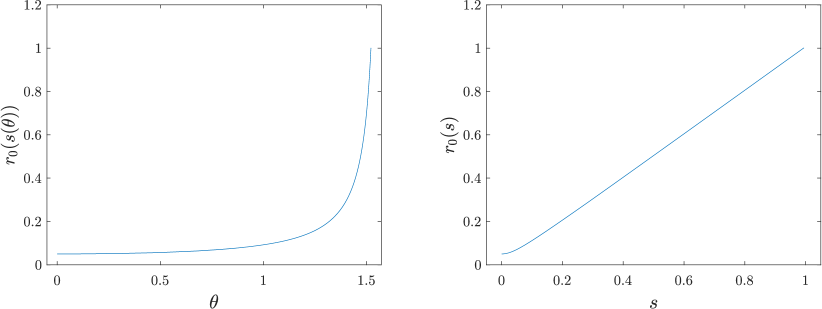
Figure 4: The mapping $r_{0}(s)$ is better-conditioned than $r_{0}(s(\theta))$. In this example, the curved side is the line segment connecting $(1,0)$ and $(1,1)$, and the origin of the polar coordinate system is $v=(0,0)$.

Observation 3.6.

It is also possible to express the double integral over $\Delta$ in polar coordinates (see formula (28)). However, when $\Delta$ is stretched, the mapping from the polar angle to the radius (i.e., $r_{0}(s(\theta))$) is ill-conditioned, while the mapping from the arc length parameter to the radius (i.e., $r_{0}(s)$) is always well-conditioned (see Figure 4).

Observation 3.7.

When the curve $\gamma$ is a line segment, it is not hard to show that the function ${\bigl{\lvert}(\gamma(s)-v)\times\gamma^{\prime}(s)\bigr{\rvert}}$ is a constant, and is equal to the distance from $v$ to $\gamma$. Furthermore, this function is also a constant when $\gamma$ is an arc of a circle centered at $v$. In general, this function turns out to be smooth except when the curve $\gamma$ is highly convex, regardless of the aspect ratio of the curved element associated with $\gamma$. It follows that the Jacobian term $\widetilde{r}\cdot{\bigl{\lvert}(\gamma(s)-v)\times\gamma^{\prime}(s)\bigr{\rvert}}$ in (26) is also a smooth function under the same conditions. Therefore, given a smooth function over a curved element $\widetilde{\Delta}$ whose curved side is well-resolved and not excessively convex, the corresponding function in radius-arc length coordinates is also smooth, regardless of the aspect ratio of $\widetilde{\Delta}$. Such a property is particularly useful for numerical integration.

Remark 3.8.

To fulfill the assumption in Theorem 3.2, it is necessary to have the polar angle of the curved side of each curved element be strictly monotone. In other words, any ray with the vertex opposite to the curved side as an endpoint cannot intersect the curved side more than once. In practice, this assumption can be easily fulfilled by a slight refinement of the mesh near the domain boundary. We note that the mesh refinement is easy to achieve by the Distmesh algorithm (see Observations A.3, A.5).

By Theorem 3.2, (24) becomes

$$\iint_{\Delta}\log({\lVert v-y\rVert})f(y)\,\mathrm{d}A_{y}$$

$$=\int_{0}^{L}\Bigl{(}\int_{0}^{1}\bigl{(}\log(r_{0}(s))+\log(\widetilde{r})\bigl{)}\cdot f\bigl{(}y(\widetilde{r},s)\bigr{)}\widetilde{r}\,\mathrm{d}\widetilde{r}\Bigr{)}{\bigl{\lvert}(\gamma(s)-v)\times\gamma^{\prime}(s)\bigr{\rvert}}\,\mathrm{d}s$$

$$=\int_{0}^{L}\bigl{(}I_{1}(s)+I_{2}(s)\bigr{)}{\bigl{\lvert}(\gamma(s)-v)\times\gamma^{\prime}(s)\bigr{\rvert}}\,\mathrm{d}s,$$ (30)

where

$$I_{1}(s)=\int_{0}^{1}\widetilde{r}\log\widetilde{r}\cdot f\bigl{(}y(\widetilde{r},s)\bigr{)}\,\mathrm{d}\widetilde{r},\quad I_{2}(s)=\int_{0}^{1}\widetilde{r}\log(r_{0}(s))f\bigl{(}y(\widetilde{r},s)\bigr{)}\,\mathrm{d}\widetilde{r}.$$ (31)

Clearly, the integrand of $I_{2}(s)$ is smooth, while the integrand of $I_{1}(s)$ has an $\widetilde{r}\log\widetilde{r}$ singularity at $\widetilde{r}=0$, which has to be resolved by our quadrature scheme. Using generalized Gaussian quadratures (see [8]), for any given $N\in\mathbbm{N}_{\geq 0}$, we can obtain a set of quadrature nodes and weights

$$\{\widetilde{r}_{j},\widetilde{w}_{j}\}_{j=1,2,\dots,N_{q}}$$ (32)

that integrates both

$$\bigl{\{}\widetilde{r}\log\widetilde{r}\cdot P_{n}(2\widetilde{r}-1)\bigr{\}}_{n=0,1,\dots,N}$$ (33)

and

$$\bigl{\{}\widetilde{r}\cdot P_{n}(2\widetilde{r}-1)\bigr{\}}_{n=0,1,\dots,N}$$ (34)

over the interval $[0,1]$ to machine precision, where $P_{n}$ represents the Legendre polynomial of order $n$. In other words, this quadrature rule integrates the space of polynomials of order $N$ over $[0,1]$ multiplied by $\widetilde{r}$ or $\widetilde{r}\log\widetilde{r}$ to machine accuracy. Therefore, the inner integral of (30) can be approximated by

$$I_{1}(s)+I_{2}(s)\approx\sum_{j=1}^{N_{q}}\widetilde{w}_{j}\widetilde{r}_{j}\log(r_{0}(s)\widetilde{r}_{j})f\bigl{(}y(\widetilde{r}_{j},s)\bigr{)},$$ (35)

from which it follows that

$$\iint_{\Delta}\log({\lVert v-y\rVert})f(y)\,\mathrm{d}A_{y}\approx\sum_{j=1}^{N_{q}}\widetilde{w}_{j}\widetilde{r}_{j}\int_{0}^{L}\log(r_{0}(s)\widetilde{r}_{j})f\bigl{(}y(\widetilde{r}_{j},s)\bigr{)}{\bigl{\lvert}(\gamma(s)-v)\times\gamma^{\prime}(s)\bigr{\rvert}}\,\mathrm{d}s$$

$$=\sum_{j=1}^{N_{q}}\widetilde{w}_{j}\widetilde{r}_{j}\int_{0}^{L}\bigl{(}\log(r_{0}(s))+\log(\widetilde{r}_{j})\bigr{)}f\bigl{(}y(\widetilde{r}_{j},s)\bigr{)}{\bigl{\lvert}(\gamma(s)-v)\times\gamma^{\prime}(s)\bigr{\rvert}}\,\mathrm{d}s.$$ (36)

To compute the integrals with respect to the arc length $s$ in (36), we first observe that $f\bigl{(}y(\widetilde{r}_{j},s)\bigr{)}\cdot{\bigl{\lvert}(\gamma(s)-v)\times\gamma^{\prime}(s)\bigr{\rvert}}$ is a smooth function of $s$ when $\gamma$ is smooth and not too convex (see Observation 3.7). Thus, all that remains is to examine the singularity of the term $\log(r_{0}(s))$. In the case where $\gamma$ denotes a line segment, it is clear that

$$r_{0}(s)=\sqrt{(s-\widetilde{s})^{2}+{\lVert v-\gamma(\widetilde{s})\rVert}^{2}}$$ (37)

for $\widetilde{s}:=\operatornamewithlimits{argmin}_{s}{\lVert v-\gamma(s)\rVert}$, from which it follows that the analytic continuation of $r_{0}(s)$ equals zero at $s=\widetilde{s}+i{\lVert v-\gamma(\widetilde{s})\rVert}$, where $i$ is the imaginary unit. Thus, when $\gamma$ is a line segment, $\log(r_{0}(s))$ has a singularity at $s=\widetilde{s}+i{\lVert v-\gamma(\widetilde{s})\rVert}$. In the case where $\gamma$ is an arbitrary curved side that is well-resolved by the mesh (which is one of our assumptions), $\gamma$ can be seen as a smooth perturbation of a line segment. If we define $\widetilde{s}$ by the formula described above for the line segment, the singularity of $\log(r_{0}(s))$ is likewise located near $s=\widetilde{s}+i{\lVert v-\gamma(\widetilde{s})\rVert}$. Below, we introduce an algorithm for resolving such a singularity.

1. Subdivide the integration interval into two pieces: $[0,\widetilde{s}]$ and $[\widetilde{s},L]$, where $\widetilde{s}=\operatornamewithlimits{argmin}_{s}{\lVert v-\gamma(s)\rVert}$.

2. Divide $[0,\widetilde{s}]$ into $N+1$ subintervals

   $$\{[(1-(1/2)^{N})\widetilde{s},\widetilde{s}]\}\bigcup\{[(1-(1/2)^{i-1})\widetilde{s},(1-(1/2)^{i})\widetilde{s}]\}_{i=1,2,\dots,N},$$ (38)

   where

   $$N=\min\{N:(1/2)^{N}\widetilde{s}<{\lVert v-\gamma(\widetilde{s})\rVert}\}.$$ (39)

3. Similarly, divide $[\widetilde{s},L]$ into $M+1$ subintervals, where

   $$M=\min\{M:(1/2)^{M}(L-\widetilde{s})<{\lVert v-\gamma(\widetilde{s})\rVert}\}.$$ (40)

4. Use the Gauss-Legendre quadrature rule of order $p$ over each subinterval to compute (36). It is necessary for $p$ to be large enough, such that the two integrals

   $$\int_{0}^{\widetilde{s}/2}\bigl{(}\log(r_{0}(s))+\log(\widetilde{r}_{j})\bigr{)}f\bigl{(}y(\widetilde{r}_{j},s)\bigr{)}{\bigl{\lvert}(\gamma(s)-v)\times\gamma^{\prime}(s)\bigr{\rvert}}\,\mathrm{d}s$$ (41)

   and

   $$\int_{(L+\widetilde{s})/2}^{L}\bigl{(}\log(r_{0}(s))+\log(\widetilde{r}_{j})\bigr{)}f\bigl{(}y(\widetilde{r}_{j},s)\bigr{)}{\bigl{\lvert}(\gamma(s)-v)\times\gamma^{\prime}(s)\bigr{\rvert}}\,\mathrm{d}s$$ (42)

   can be computed to full accuracy.

Using the subdivision technique presented above, it is guaranteed that each panel is separated from the singularity by at least one panel width, such that it is in the far field of the logarithmic singularity. It follows that an accurate quadrature result is obtained.

Remark 3.9.

The adaptive subdivision along the arc length coordinate for resolving the nearly-singular integrand can be expensive, especially when the target is close to the boundary. One can instead use a large number of precomputed specialized quadrature rules to resolve the nearly-singular integrand, which is substantially more efficient than the adaptive integration method described above (see [6, 7]). In our implementation, for simplicity, we compute the self-interactions using the adaptive integration method.

Remark 3.10.

The need for subdivisions in the arc length coordinate is not an artifact of the change of variables, since when the target location $v$ is close to the edge of a mesh element, the integrand is in nature nearly-singular along the arc-length direction in the region between $v$ and that edge.

3.5 Interpolation over a mesh element

In this section, we describe an interpolation scheme of the volume potential (15) over a mesh element. We note that the volume potential is smooth provided that the boundary of the domain $\partial\Omega$ and the density $f$ is smooth (see, for example, [29]), from which it follows that the Koornwinder polynomial basis is suitable for the interpolation of the volume potential in this case.

First of all, given a mesh element $\Delta$ and an invertible and well-conditioned mapping $\rho$ from the standard simplex $\Delta^{1}$ to $\Delta$ (see Section 3.1 for the construction of $\rho$), the Koornwinder polynomial expansion coefficients of the function $u\circ\rho:\Delta^{1}\to\mathbbm{R}$ can be computed by applying the interpolation matrix to the values of $u$ at the Vioreanu-Rokhlin nodes over $\Delta$ (see Section 2.2), and we denote the interpolant by $I_{u\circ\rho}$. As $u\circ\rho$ is a smooth function and $\rho$ is easily invertible (the use of Newton’s method is necessary when $\Delta$ is a curved element), we can compute the potential to high accuracy at any point on $\Delta$ by evaluating $(I_{u\circ\rho})\circ\rho^{-1}$.

Remark 3.11.

In some applications, it is useful to compute the volume potentials at the boundary of the domain, i.e., the value of $u(v)$ for some $v=\gamma(s)$, where $\gamma$ is the arc length parameterization of the curved side of the curved element that $v$ lies in. In this case, the use of Newton’s method is unnecessary, since it is easy to show that $\rho^{-1}(v)=(1-s/L,0)$, where $\rho$ is the blending function mapping (18), and $L$ is the total arc length of $\gamma$.

Observation 3.12.

As is noted in Observation 3.2, when the curved side of a curved element is not well-resolved by the mesh, the Jacobian of $\rho$ could be nonsmooth. Thus, it is important for the curved side to be well-resolved by the mesh, or, if it is not well-resolved, to use a higher-order interpolation scheme.

3.6 Coupling quadratures to the FMM

With the numerical apparatus developed in the previous sections, given geometry with a triangle mesh, and a source function $f:\mathbbm{R}^{2}\to\mathbbm{R}$, we can evaluate the integral (15) at any given target location in $\mathcal{O}(N)$ operations, where $N$ is the total number of the quadrature nodes, by summing up all of the potentials generated over the mesh elements at the target location, using the algorithms introduced in Sections 3.2, 3.3, 3.4. It is not hard to see that the cost is dominated by the far field interactions.

It is often desirable to evaluate the potential at multiple targets, which, if computed naively, leads to $\mathcal{O}(MN)$ total operations, where $M$ is the number of target locations. Such an expensive cost is usually prohibitive in practice. In this section, we reduce the time complexity to $\mathcal{O}(M+N)$ by coupling the FMM to our volume potential evaluation algorithm.

The key observation of the algorithm is that, if we treat all interactions as far field interactions, the volume potential evaluation is equivalent to a standard electrostatic interaction problem, where the charge locations are the quadrature nodes over the triangles, and the charge densities are given by the density function values at the nodes multiplied by the corresponding quadrature weights. Therefore, with the well-known fast multipole method [15], such computations can be done with linear time complexity. However, since treating all quadrature nodes as point sources does not account for the near and self-interactions, the computed potential is inaccurate. Therefore, it is necessary to make a correction to the computed potential. Below, we outline the so-called “subtract-and-add” method (see [16]) for the potential corrections.

Suppose that $x$ is a target location, and $u(x)$ is the potential at $x$ computed using the FMM. Let $\mathcal{S}(x)$ denote the element containing $x$, $\mathcal{N}(x)$ denote the near field of $x$, as defined in Definition 3.2.

1. Find the mesh element $\mathcal{S}(x)$ that $x$ lies within, and the set of nearby elements $\mathcal{N}(x)$ using the query algorithm described in Appendix A.5.

2. Subtract from $u(x)$ the contribution made in the FMM calculation from the quadrature nodes over $\mathcal{N}(x)$ and $\mathcal{S}(x)$. Then, add to $u(x)$ the near and self-interaction potential over $\mathcal{N}(x)$ and $\mathcal{S}(x)$, respectively, using the algorithms described in Sections 3.3 and 3.4.

Since the number of mesh elements in the near field of a given target is $\mathcal{O}(1)$, we have that the number of operations required to correct the potential at each target is $\mathcal{O}(1)$. Therefore, the total time complexity of the algorithm is still $\mathcal{O}(M+N)$.

Remark 3.13.

Clearly, the subtraction of spurious contributions from near fields can be avoided by disabling the computation of neighbor interactions in the FMM. However, it is observed in [16] that the use of the “subtract-and-add” method described in this Section leads to faster implementation, largely because of a better cache utilization. We note that catastrophic cancellation could happen during the “subtract-and-add” stage. In our case, the singularity of the logarithmic kernel is so mild that this is generally not a concern. When a more singular kernel is in use, one should omit the computation of neighbor interactions in the FMM, and handle these interactions using the algorithms of Sections 3.3, 3.4.

4 Accelerating potential evaluation over unstructured meshes

The algorithm described thus far, while differing in some details, involves fairly standard ideas that have been developed for the evaluation of the surface potential [6, 16]. In this section, we describe three general observations that lead to accelerated volume potential calculations over unstructured meshes. The first concerns the geometry of the near field. We observe that the near field is typically approximated by a ball or a triangle (see, for example, [6, 16, 1]), while in reality, the geometry of the near field can be characterized precisely by the union of several Bernstein ellipses. Moreover, these ellipses are very flat when the order of the far field quadrature rule is high, or when the error tolerance is large, from which it follows that the conventional approximations of the near field become inaccurate. When the near field is computed accurately, the cost of the most expensive component in the volume potential evaluation algorithm, namely, the near interaction potential correction, is reduced substantially. The second observation is that, knowing the near field geometry, one can efficiently offload the near field interaction corrections onto the FMM-based far field interaction computation by increasing the order of the far field quadrature rule. Such a trade leverages the computational efficiency of highly optimized parallel FMM libraries, and reduces the cost of the much more expensive and unstructured near field interaction computation. The third observation is that the most commonly used arrangement, in which the interpolation nodes are placed on the same mesh over which the potential is integrated over, leads to an artificially large potential correction cost. If the quadrature mesh and the interpolation mesh are instead staggered to one another, the number of interpolation nodes at which the near field and self-interactions are expensive to evaluate is reduced dramatically.

We present these techniques in the context of completely unstructured meshes, and note that the ideas are equally applicable in the context of hybrid or structured meshes.

4.1 Precise near field geometry analysis

In this section, we present the precise characterization of the geometry of the near field, the use of which eliminates the unnecessary near field interaction computations, and provides an error control functionality to the far and near field interaction computations.

By Definition 3.1, given a triangle integration domain $\overline{\Delta}$, a set of possible densities $S$, a far field quadrature rule $\{y_{i},w_{i}\}_{i=1,2,\dots,M}$ over $\overline{\Delta}$ of order $N$ with length $M$, and an error tolerance $\varepsilon$, the far field of $\overline{\Delta}$ is the set of points

$$\mathcal{F}_{\overline{\Delta}}=\{x\notin\overline{\Delta}:{\biggl{\lvert}\sum_{i=1}^{M}w_{i}\log{\lVert x-y_{i}\rVert}f(y_{i})-\iint_{\overline{\Delta}}\log{\lVert x-y\rVert}f(y)\,\mathrm{d}A_{y}\biggr{\rvert}}<\varepsilon,f\in S\},$$ (43)

and the near field of $\overline{\Delta}$, which we denote by $\mathcal{N}_{\overline{\Delta}}$, equals the complement of $\mathcal{F}_{\overline{\Delta}}$ in the set $\mathbbm{R}^{2}\setminus\overline{\Delta}$.

For simplicity, we assume that $\overline{\Delta}$ is the standard simplex $\Delta^{1}$. Given an arbitrary point $x_{0}=(a,b)\in\mathcal{F}_{\Delta^{1}}$, we rewrite the integrand as a Koornwinder polynomial expansion

$$R(y):=\log{\lVert x_{0}-y\rVert}f(y)=\sum_{n=0}^{\infty}\sum_{m=0}^{n}a_{mn}K_{mn}(y),$$ (44)

where $a_{mn}$ is the inner product between $f$ and $K_{mn}$ over $\Delta^{1}$. Furthermore, by definition (43), we have that

$${\biggl{\lvert}\sum_{i=1}^{M}w_{i}R(y_{i})-\iint_{\Delta^{1}}R(y)\,\mathrm{d}A_{y}\biggr{\rvert}}<\varepsilon.$$ (45)

By assumption, the far field quadrature rule $\{y_{i},w_{i}\}_{i=1,2,\dots,M}$ integrates Koornwinder polynomials of order up to $N$ exactly, from which it follows that

$$\sum_{i=1}^{M}w_{i}\sum_{n=0}^{N}\sum_{m=0}^{N-n}a_{mn}K_{mn}(y_{i})=\iint_{\Delta^{1}}\sum_{n=0}^{N}\sum_{m=0}^{N-n}a_{mn}K_{mn}(y)\,\mathrm{d}A_{y}.$$ (46)

Thus, by combining (46) and the orthogonality of the Koornwinder polynomials (see (6)), the inequality (45) becomes

$${\biggl{\lvert}\sum_{i=1}^{M}w_{i}\cdot R_{N}(y_{i})\biggr{\rvert}}<\varepsilon,$$ (47)

where

$$R_{N}(y):= \,\sum_{n=0}^{\infty}\sum_{m=0}^{n}a_{mn}K_{mn}(y)-\sum_{n=0}^{N}\sum_{m=0}^{N-n}a_{mn}K_{mn}(y)$$

$$= \,\sum_{n={\lceil(N+1)/2\rceil}}^{\infty}\sum_{m=N-n+1}^{n}a_{mn}K_{mn}(y)$$ (48)

denotes the remainder, i.e., the sum of the expansion terms with order larger than $N$. Since the remainder $R_{N}(y)$ is a general function, it is generally true that (47) holds if and only if

$${\bigl{\lvert}w_{i}\cdot R_{N}(y_{i})\bigr{\rvert}}<\varepsilon,$$ (49)

for all $i$. Specifically, the inequality (49) holds only if

$${\bigl{\lvert}R_{N}(y_{j})\bigr{\rvert}}<\frac{\varepsilon}{w},$$ (50)

where $\{y_{j}\}$ denotes the $\sim n/2$ nodes that are closest to $[0,1]\times\{0\}$, and $w$ denotes the largest quadrature weight corresponding to these nodes (we note that there are usually around $n/2$ Xiao-Gimbutas nodes along $[0,1]\times\{0\}$). By continuity of the remainder $R_{N}$, (50) implies that

$${\bigl{\lVert}R_{N}|_{[0,1]\times\{0\}}\bigr{\rVert}}_{L^{\infty}}<\varepsilon\cdot C_{N}/w,$$ (51)

where $R_{N}|_{\partial\Delta^{1}}$ is the trace of the remainder $R_{N}$ on the edges of the standard simplex $\Delta^{1}$, and $C_{N}$ is a constant that converges down to $1$ as $N$ increases, by continuity of $R_{N}$. We postpone the discussion on the actual value of $C_{N}$ to Observation 4.1.

Without loss of generality, we only consider the trace of $R_{N}$ on the edge connecting the two points $(0,0)$ and $(1,0)$, i.e., $R_{N}\big{|}_{[0,1]\times\{0\}}$. Furthermore, for ease of presentation, we map its domain to $[-1,1]$ by defining $H_{N}:[-1,1]\to\mathbbm{R}$, where

$$H_{N}(x):=R_{N}\big{|}_{[0,1]\times\{0\}}\Bigl{(}\frac{x+1}{2}\Bigr{)}.$$ (52)

Similarly, we can define the trace of the integrand $R$ (see (44)) on the same edge (after the same linear transformation of the domain) by $H:[-1,1]\to\mathbbm{R}$, where

$$H(x):=R\big{|}_{[0,1]\times\{0\}}\Bigl{(}\frac{x+1}{2}\Bigr{)}=\log{\Bigl{\lvert}a+ib-\frac{x+1}{2}\Bigr{\rvert}}\cdot f\Bigl{(}\frac{x+1}{2}\Bigr{)},$$ (53)

and $i$ is the imaginary unit (recall that $a,b$ denote the $x,y$-coordinates, respectively, of the given point $x_{0}$). Clearly, $H-H_{N}$ is the projection of $H$ onto the space of one-dimensional polynomials of order $N$.

With $H$ and $H_{N}$ thus defined, (51) can be rewritten as

$${\bigl{\lVert}H_{N}\bigr{\rVert}}_{L^{\infty}[-1,1]}<\varepsilon\cdot C_{N}/w.$$ (54)

We now define a Bernstein ellipse $E_{\rho_{0}}$ with parameter

$$\rho_{0}=\bigl{(}\frac{w}{\varepsilon\cdot C_{N}}\bigr{)}^{1/N}.$$ (55)

It is clear that $E_{\rho_{0}}$ is well-defined for sufficiently small $\varepsilon$ (so that $\rho_{0}>1$). Then, we have that $H-H_{N}$ is a one-dimensional polynomial of order $N$ approximating $H$, satisfying

$${\lVert H-(H-H_{N})\rVert}_{L^{\infty}[-1,1]}={\lVert H_{N}\rVert}_{L^{\infty}[-1,1]}<\varepsilon\cdot C_{N}/w=\rho_{0}^{-N},$$ (56)

by (54) and (55). It follows that, by Theorem 2.3,

$$H(z)=\log{\Bigl{\lvert}a+ib-\frac{z+1}{2}\Bigr{\rvert}}\cdot f\Bigl{(}\frac{z+1}{2}\Bigr{)}$$ (57)

can be analytically continued to an analytic function in the open Bernstein ellipse $E_{\rho_{0}}$. Therefore, we have that the complex number $2(a+ib)-1$ must be outside of $E_{\rho_{0}}$. Equivalently, in the Cartesian plane, the point $x_{0}$ has to be outside of

$$E_{\rho_{0}}^{(1)}:=\Bigl{\{}\Bigl{(}\frac{x+1}{2},\frac{y}{2}\Bigr{)}:x+iy\in E_{\rho_{0}}\Bigr{\}}.$$ (58)

Similarly, one can apply the same argument to the remaining two edges of $\Delta^{1}$, and get two more ellipses, which we denote by $E_{\rho_{0}}^{(2)}$ and $E_{\rho_{0}}^{(3)}$. It follows that it is a necessary condition that the near field $\mathcal{N}_{\Delta^{1}}$ contains the union of the three ellipses in $\mathbbm{R}^{2}\setminus\Delta^{1}$, i.e.,

$$E_{\Delta^{1}}\subset\mathcal{N}_{\Delta^{1}},$$ (59)

where

$$E_{\Delta^{1}}:=\bigl{(}\cup_{i=1}^{3}E_{\rho_{0}}^{(i)}\bigr{)}\setminus\Delta^{1}.$$ (60)

In other words, $E_{\Delta^{1}}$ is a lower bound of the near field $\mathcal{N}_{\Delta^{1}}$. One could, in fact, apply the same argument to get an ellipse for every line segment inside $\Delta^{1}$, however, it is clear that their union in $\mathbbm{R}^{2}\setminus\Delta^{1}$ equals $E_{\Delta^{1}}$. Thus, $E_{\Delta^{1}}$ is the optimal lower bound that we can obtain using our argument. Furthermore, it turns out that, with some additional mild assumptions, one can show that the lower bound $E_{\Delta^{1}}$ is tight, and we sketch the proof below.

Firstly, we define a union of three Bernstein ellipses that are slightly larger than $E_{\Delta^{1}}$:

$$E_{\Delta^{1}}^{\prime}:=\bigl{(}\cup_{i=1}^{3}E_{C_{N}^{1/N}\cdot\rho_{0}}^{(i)}\bigr{)}\setminus\Delta^{1}.$$ (61)

We note that the factor $C_{N}^{1/N}$ converges down to $1$ as $N$ increases, and that empirically, $C_{N}$ is small when $N$ is small (see Table 1).

Given $x_{0}\in\mathbbm{R}^{2}\setminus(\Delta^{1}\cup E_{\Delta^{1}}^{\prime})$, suppose that the restriction of the integrand $R$ to any line segment inside $\Delta^{1}$ can be analytically continued inside $\Delta^{1}\cup E_{\Delta^{1}}^{\prime}$. Suppose further that the analytic continuation of each such restriction is bounded inside $\Delta^{1}\cup E_{\Delta^{1}}^{\prime}$ by $1/4$. Also note that in practice, the parameter $\rho_{0}$ is generally larger than $1.5$ (see formula (55), Observation 4.1). We want to show that $x_{0}\in\mathcal{F}_{\Delta^{1}}$.

Recall that $x_{0}\in\mathcal{F}_{\Delta^{1}}$ if

$${\bigl{\lvert}R_{N}(y_{i})\bigr{\rvert}}<\frac{\varepsilon}{w_{i}},$$ (62)

for all $i$ (see formulas (48), (49)). We show that (62) holds for all the quadrature nodes $\{y_{i}\}$ by considering two cases, one for the $\sim 3\cdot n/2$ nodes that are closest to $\partial\Delta^{1}$, and the other for the rest of the nodes, which are away from $\partial\Delta^{1}$.

Proof for $\{y_{i}\}$ that are close to $\partial\Delta^{1}$:

By Corollary 2.5, we have that

$${\lVert R_{N}\rVert}_{L^{\infty}([0,1]\times\{0\})}={\lVert H_{N}\rVert}_{L^{\infty}[-1,1]}\approx{\lVert H-f_{N}\rVert}_{L^{\infty}[-1,1]}\leq(C_{N}^{1/N}\cdot\rho_{0})^{-N}=\varepsilon/w,$$ (63)

where $f_{N}$ denotes the Chebyshev projection of $H$ of order $N$. By a similar argument, one can show that

$${\lVert R_{N}\rVert}_{L^{\infty}([0,1]\times\{y\})}\leq\varepsilon/w\leq\varepsilon/w_{i},$$ (64)

for all $y$ close to zero, and for all quadrature weights $w_{i}$ corresponding to the nodes $y_{i}$ that are close to $[0,1]\times\{0\}$. Therefore, we have that (62) holds for all the $\sim n/2$ nodes $y_{i}$ that are closest to the line segment connecting $(0,0)$ and $(1,0)$. Similarly, one can show that (62) holds for all the $\sim 3\cdot n/2$ nodes that are closest to the three sides of $\Delta^{1}$.

Proof for $\{y_{i}\}$ that are away from $\partial\Delta^{1}$:

We observe that, in practice (i.e., when the order $N$ of the quadrature rule is no larger than $50$), all the quadrature weights $\{w_{i}\}$ are bounded by $10\cdot w$. Therefore, to prove (62), it is sufficient to show that

$${\bigl{\lvert}R_{N}(y)\bigr{\rvert}}<\frac{\varepsilon}{10\cdot w},$$ (65)

for $y\in\Delta^{1}$ that are away from $\partial\Delta^{1}$. Numerically, given an arbitrary line segment $L$ inside $\Delta^{1}$, provided that the mapping from $\{K_{mn}|_{L}\}_{0\leq m+n\leq N}$ to $\{T_{n}\}_{n=1,2,\dots,N}$ is stable (where $T_{n}$ denotes the Chebyshev polynomial of order $n$),

$${\lVert R_{N}|_{L}\rVert}<\frac{\varepsilon}{10\cdot w}$$ (66)

holds if and only if

$${\lVert R|_{L}-f_{n}\rVert}<\frac{\varepsilon}{10\cdot w}$$ (67)

holds, where $f_{n}$ is the $n$th order Chebyshev projection of $R|_{L}$. Clearly, for each $y\in\Delta^{1}$, one can pick a sufficiently long line segment $L$ that contains $y$, such that the mapping is stable. Then, by Corollary 2.5, the inequality (67) (equivalently, (66)) holds if $x_{0}$ is outside a Bernstein ellipse transformed so that the interval $[-1,1]$ corresponds to $L$, with parameter $(10\cdot w/\varepsilon)^{1/N}$. It is easy to see that such an ellipse is inside $E_{\Delta^{1}}\cup\Delta^{1}$. Thus, by definition of $x_{0}$, the inequality (65) holds for all $y\in\Delta^{1}$ that are away from $\partial\Delta^{1}$.

Therefore, (62) holds for all $i$, from which it follows that $x_{0}\in\mathcal{F}_{\Delta^{1}}$, and $E_{\Delta^{1}}$ is a tight lower bound of the near field when $C_{N}^{1/N}$ is close to $1$.

Observation 4.1.

Empirically, we find that, when $f\in S$ is sufficiently smooth over the integration domain (a triangle), and when $C_{N}$ is chosen according to Table 1, the set $E_{\Delta^{1}}$ precisely characterizes the near field of the standard simplex $\Delta^{1}$ (see Figures 6, 7, 8).

$N$	50	40	30	25	20	12
$C_{N}$	1	2	2.5	3	6.8	12

Table 1: The values of $C_{N}$ that allow $E_{\Delta^{1}}$ to characterize the near field of $\Delta^{1}$ precisely. We note that this table is obtained empirically, and the values work for arbitrary triangles. Furthermore, the table agrees with the claim that $C_{N}$ converges down to $1$ as $N$ increases.

To generalize this argument to arbitrary triangles, one only needs to adjust the constant $w$ (see (50)) based on the magnitude of the quadrature weights (equivalently, the size of the triangle). This, however, does not add difficulty to the implementation, since one only needs to compute $w$ for the standard simplex once, and then scale it according to the ratio between the area of the triangle and the area of the standard simplex. We note that the naive estimation of the near field neglects this nonlinear relation between the size of the near field and the size of the mesh element, which causes unnecessary near field interaction computations, especially when the mesh element is small. Apart from this, it is important to note that, given a stretched triangle, $E_{\Delta^{1}}$ may not be the optimal lower bound that we can obtain using our argument. For example, as is shown in the left part of Figure 6(d), the near field corresponding to the error tolerance $10^{-14}$ is not perfectly captured by $E_{\Delta^{1}}$. Such an issue can be fixed by adding the ellipse, obtained from applying our argument to the line segment connecting $(0,0.5)$ and $(4,0.5)$, to the union of ellipses. In practice, stretched triangles rarely appear if a decent meshing algorithm is used, and the presence of a few stretched triangles barely affects the overall accuracy of the evaluation.

In the situation where the domain is a curved element, if the mapping from the reference domain (i.e., a standard simplex) to the curved element is also valid and sufficiently smooth for points near the simplex, one can apply our argument to the reference domain, and compute the inverse mapping of any given point outside the curved element (by Newton’s method) to check whether the point is inside the near field or not; Alternatively, one could linearize the curved boundary of the curved element with a polyline, and apply our argument to every linearized boundary segment (adjusting $\varepsilon$ to account for the numerically smaller polynomial orders on the traces). We note that, in practice, given a curved element, very few discretization nodes that are close to the curved side belong to the near field of the curved element, and thus, it is often convenient to to treat the curved side as a straight line segment when one applies the near field geometry analysis.

Besides allowing for the precise identification of all of the necessary near interaction potential corrections, we note that our near field geometry analysis is also helpful in the near field interaction computation itself. Recall that, in Section 3.3, we describe an adaptive algorithm for resolving the nearly-singular integrand, which recursively subdivides the integration domain, such that the integrand is smooth on each subdomain. When our near field geometry analysis is applied to the subdomains, the algorithm is able to decide the number of required subdivisions precisely, avoiding the possibility both of oversampling and undersampling.

Observation 4.2.

The shape of a near field is similar to a circle, when both the error tolerance and the order of the quadrature rule are low (see Figures 6(a) and 8(a)). This, however, does not imply that our estimation is useless in such a setting. Firstly, without rigorous analysis, one often needs to overestimate the size of the near field to improve the robustness of the algorithm. Secondly, in the adaptive subdivision-based near field interaction computation, as in the case of arbitrary triangles, one has to scale the size of $w$ as the area of the triangle becomes smaller during the subdivisions, which is equivalent to increasing the error tolerance $\varepsilon$ by (55). One can observe from Figure 8(a) that the naive estimation of the near field of the sub-triangle becomes inefficient, and leads to many unnecessary subdivisions.

Remark 4.3.

By formulas (55) and (60), the volume of the near field goes to zero as the order of the far field quadrature rule goes to infinity. The near field estimated by a ball, on the other hand, always results in a non-negligible volume. Moreover, we note that, the more distorted a mesh element is, the poorer the naive estimation of its near field becomes.

Remark 4.4.

The shape information of the ellipses can be efficiently precomputed for all the mesh elements. Thus, the cost of checking whether a target is inside the approximated near field or not using ellipses is negligible.

We report the true near field and our estimated near field, for different triangles with different densities and different quadrature orders, in Section 5.1.1. We also report the performance of the volume potential evaluation algorithm, with and without precise near field geometry analysis, in the same section.

4.2 Offloading the near field interaction computation onto the FMM-based far field interaction computation

Since the volume of the near field goes to zero as the order of the far field quadrature rule increases (see Remark 4.3), the number of near field interaction potential corrections can be reduced arbitrarily, in exchange for a more expensive far field interaction computation. It has been long realized that one needs to adjust the order of the far field quadrature rule, such that the costs of the far field interactions and the near field interactions are balanced (see, for example, [1, 16]). However, this idea is presented as a heuristic in the literature, and the adjustments are done empirically. In fact, without characterizing the near field geometry precisely, such an idea cannot be efficiently carried out. This is because, when the order of the far field quadrature rule is high, the standard approximation of the near field by a ball or a triangle becomes inaccurate (see Section 4.1 and Figure 6). It follows that the high-order far field quadrature rule is underutilized; moreover, one has to overestimate the size of the near field to improve the robustness of the algorithm, in the absence of the precise near field geometry analysis. Therefore, the use of the precise near field geometry analysis is critical for efficiently offloading the near field interaction computation onto the FMM-based far field interaction computation.

To quantify the trade-off, we analyze the rate at which the Bernstein ellipse $E_{\rho_{0}}$ shrinks. It is easy to show that the area of a Bernstein ellipse with parameter $\rho$ is asymptotically proportional to

$$\log\rho_{0}=\frac{1}{N}\log\bigl{(}\frac{w}{\varepsilon\cdot C_{N}}\bigr{)},$$ (68)

(see, for example, [10]), from which it follows that the cost of the near field interaction potential corrections is proportional to

$$\frac{3}{N}\log\bigl{(}\frac{w}{\varepsilon\cdot C_{N}}\bigr{)}.$$ (69)

We also have that the cost of the FMM-based far field interaction computation is proportional to

$$N_{tgt}+N_{src}=N_{tgt}+\mathcal{O}(N^{2}),$$ (70)

where $N_{tgt},N_{src}$ denote the number of the target locations and the number of quadrature nodes in total, respectively. Despite that the FMM cost can potentially increase at a faster rate than the near field interaction potential correction cost decreases, such a trade leverages the computational efficiency of highly optimized parallel FMM libraries (see, for example, [22, 31]), and reduces the cost of the much more expensive and unstructured near field interaction computation. In practice, we find that the FMM cost increases much more slowly, since the number of the interpolation nodes tends to be large compared to the number of the quadrature nodes of the same order, from which it follows that the FMM cost is dominated by the large number of target points, unless the order of the far field quadrature rule is extremely high (see Figure 10). In addition, although the near field interaction (and self-interaction) potential corrections are embarrassingly parallelizable, and their costs can be potentially made very small with the use of many cores, it still requires engineering efforts to attain the optimal parallel efficiency. On the other hand, many efforts have been made in the design and implementation of parallel FMM libraries, and thus, it is preferable to offload the near field interaction computations onto the far field interaction computations.

Remark 4.5.

We use high order far field quadrature rules in this paper to resolve the Green’s function, rather than the density function. It follows that the density function can be oversampled during the integration process, which is undesirable when its evaluation is expensive. In this situation, it is recommended to construct a lower-order interpolant of the density function.

We demonstrate the effectiveness of the offloading technique in Section 5.1.2.

4.3 Fast interpolation of the volume potential with a staggered mesh

In Section 3.5, we described an interpolation scheme for the volume potential over a mesh element. In practice, it is often desirable to have the volume potential interpolated over all the mesh elements in the domain $\Omega$, such that the evaluation of the volume potential at any point in the domain is both instantaneous and accurate. A common strategy is to let a single mesh serve both as the quadrature mesh and the interpolation mesh, i.e., the interpolants are constructed by evaluating the volume potential at the Vioreanu-Rokhlin nodes over all mesh elements, and the integration domain $\Omega$ is discretized into the same set of the mesh elements. In this section, we first show that such an approach does not lead to optimal computational efficiency. Then, we propose a simple modification that significantly improves the efficiency.

First of all, we note that the time cost of the potential correction is strongly correlated with the location of the target: if the target is extremely close to some edge in the mesh, extensive subdivisions are required to resolve the near-singularity in the near and self-interactions (see Sections 3.3, 3.4 for details); if the target is away from all of the edges, e.g., in the center of a mesh element, very few subdivisions are required and the correction can be made rapidly. Therefore, when a single mesh is both used for quadrature and interpolation, the potential corrections become very expensive, since the interpolation nodes tend to cluster around the edges and corners of the mesh elements (see Figure 5). Furthermore, the precise identification of the near field and the offloading technique (described in Sections 4.1, 4.2) become less helpful if the majority of the nodes nearby a mesh element are indeed inside its near field.

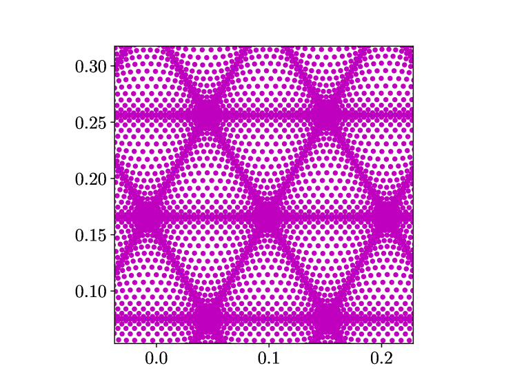
Figure 5: Interpolation nodes over a mesh. Note that the nodes cluster around the edges.

However, it is important to note that the non-uniform potential correction cost described above is an artifact of the discretization of the domain (see Appendices A.3, A.4), rather than an intrinsic difficulty of the problem. We observe that if one instead staggers the interpolation mesh with the quadrature mesh, both the number of potential corrections for each target, and the number of subdivisions needed for resolving the nearly-singular integrands, are reduced substantially. By “stagger”, we mean that the edges of the interpolation mesh are maximally non-overlapping with the edges of the quadrature mesh, such that the interpolation nodes cluster around the centroid of each element in the quadrature mesh (see Figure 9).

A good heuristic approximation to such an interpolation mesh can be obtained by shifting the initial guess to the meshing algorithm (the triangular tiling, see Appendix A.3), such that the initial guess for the interpolation mesh becomes staggered with the initial guess for the quadrature mesh.

We report the performance of the interpolation, with and without the use of a staggered mesh, in Section 5.1.1.

Remark 4.6.

With the use of a staggered mesh, some target points could be extremely close to some edges in the mesh. As is shown in Tables 5 and 6, this turns out not to be a problem, since the number of required subdivisions increases logarithmically with respect to the distance between the target point and the edges, and such targets only make up a small proportion of the total target points.

5 Numerical experiments

In this section, we illustrate the performance of the algorithm with several numerical examples. We implemented our algorithm in FORTRAN 77, and compiled it using the Intel Fortran Compiler, version 2021.5.0, with the -Ofast flag. We conducted all experiments on a ThinkPad laptop, with 16 GB of RAM and an Intel Core i7-10510U CPU. We note that, in our implementation, we do not construct interpolants of the density function, but rather always evaluate the density function naively. Thus, the timing results that we present depend on the actual cost of evaluating the density functions. Furthermore, for simplicity, we numerically reparametrize the input parametrized curve (i.e., the boundary of the domain $\Omega$) by arc length, which results in a somewhat costly evaluation of the reparametrized curve. This, however, does not affect the spirit of the experimental results that we present, i.e., the acceleration of the computation using the techniques described in this paper.

We use the code that is publicly available in the companion code of [6] for the evaluation of Koornwinder polynomials. We also use the tables of Xiao-Gimbutas rules and Vioreanu-Rokhlin rules that are publicly available in [12]. We use the FMM library published in [11] in our implementation. We make no use of the high-performance linear algebra libraries, e.g., BLAS, LAPACK, etc.

We list the notations that appear in this section below.

• $h_{0}$: the mesh element size.

• $\varepsilon$: the error tolerance of the far and near field interaction computations (controlled by the precise near field geometry analysis).

• $N$: the order of the quadrature rule. In particular, we use the following notations to denote the value under the special settings.

  • $N_{f}$: the order of the far field quadrature rule.

  • $N_{n}$: the order of the quadrature rule used in the near field interaction computation.

  • $N_{l}$: the order of the Gauss-Legendre quadrature rule used in the self-interaction computation (along the arc length coordinate).

  • $N_{g}$: the order of the generalized Gaussian quadrature rule used in the self-interaction computation (along the radial coordinate), in the sense that it integrates both $\phi(r)$ and $r\log r\cdot\phi(r)$ over $[0,1]$ exactly, where $\phi(r)$ is a polynomial of order up to $N_{g}$.

  • $N_{s}$: the order of the interpolation scheme.

• $N_{\textit{tot}}$: the total number of discretization nodes.

• $c$: the average number of the potential corrections (including corrections both over triangles and curved elements), for each target location.

• $s_{n}$: the average number of subtriangles that one needs to integrate over, to resolve the nearly-singular integrands in the near field interaction computations, including both the triangle and curved element integration domains, for each target location.

• $s_{l}$: the total number of subdivisions along the arc length coordinate to resolve the nearly-singular integrands in the self-interaction computations.

• $T_{\mathcal{F}}$: The time spent on far field interaction computations.

• $T_{\mathcal{N}}$: The time spent on near field interaction computations.

• $T_{\mathcal{F}+\mathcal{N}}$: The total time spent on far and near field interaction computations.

• $T_{\mathcal{S}}$: The time spent on self-interaction computations.

• $T_{tot}$: The total time for the evaluation of the volume potential at all of the discretization nodes.

• $E_{\textit{abs}}$: the largest absolute error of the potential evaluations at all of the interpolation nodes.

• $\widetilde{E}_{\textit{abs}}$: the largest absolute error of the solution to Poisson’s equation at all of the interpolation nodes.

• $\frac{\#\textit{tgt}}{\textit{sec}}$: the number of targets that the algorithm (with the use of precise near field geometry analysis and a staggered mesh) can evaluate the volume potential at, per second.

We list the superscripts that appear in the notations below.

• $0$ (e.g., $c^{0},s_{n}^{0}$): the experimental setting where the near field is approximated naively by a ball, and the staggered mesh is not used.

• $+$ (e.g., $c^{+},s_{n}^{+}$): the experimental setting where the near field is approximated by the union of Bernstein ellipses, and the staggered mesh is not used.

• $*$ (e.g., $c^{*},s_{n}^{*}$): the experimental setting where the near field is approximated by the union of Bernstein ellipses, and the staggered mesh is used.

• quad (e.g., $N_{\textit{tri}}^{\textit{quad}}$, $N_{\textit{tot}}^{\textit{quad}}$): the quadrature mesh-related information.

• interp (e.g., $N_{\textit{tri}}^{\textit{interp}}$, $N_{\textit{tot}}^{\textit{interp}}$): the interpolation mesh-related information.

In Tables 2 and 3, we tabulate the orders and lengths of the quadrature rules used in our implementation.

Type	$N_{f}$	Length
X-G	12	32
X-G	33	201
X-G	40	290
X-G	50	444
GGQ	8	8

Table 2: The orders and lengths of the quadrature rules. We note that X-G denotes the Xiao-Gimbutas rules, and GGQ denotes the generalized Gaussian quadrature rule that we make use of in Section 3.4.

$N_{s}$	$N_{f}$	Length	$\kappa$
12	20	91	19.2
20	33	231	194

Table 3: The orders, lengths and condition numbers of the Vioreanu-Rokhlin rules. We denote the condition number of the interpolation matrix by $\kappa$.

5.1 Effectiveness of the acceleration techniques

In this section, we demonstrate the effectiveness of the acceleration techniques described in Section 4. We fix $N_{n}=12$, $N_{l}=16$, $N_{g}=8$ (in fact, the values of $N_{l}$ and $N_{g}$ are irrelevant to the experimental results presented in this Section, as we only report the number of subdivisions).

5.1.1 Precise near field estimation and staggered mesh-based interpolation

In this section, we first demonstrate how well the near field is characterized by the union of Bernstein ellipses in Figures 6, 7, 8. Additionally, we provide an illustration of two staggered meshes in Figure 9. Then, we report the effect of the near field geometry analysis and the use of a staggered mesh on the average number of near field potential corrections, and the average number of the subtriangles that one needs to integrate over, for each target, in Table 5. In Table 6, we also report the number of subdivisions along the arc length coordinate in the computation of self-interactions, with and without the use of a staggered mesh.

To estimate the errors, we consider the computation of

$$u(x)=\iint_{\Omega}\frac{1}{2\pi}\log({\lVert x-y\rVert})\,\mathrm{d}A_{y},$$ (71)

where the integration domain $\Omega$ is a circle with radius $1$. In Table 4, we report the size of this problem for varioius mesh sizes $h_{0}$. It can be easily shown that $u(x)=\frac{1}{4}({\lVert x\rVert}^{2}-1)$. Again, we note that the cost of evaluating the density function is independent of the experimental results that we present here, as we only report the number of corrections and subtriangles that one needs to integrate over, rather than the actual time costs.

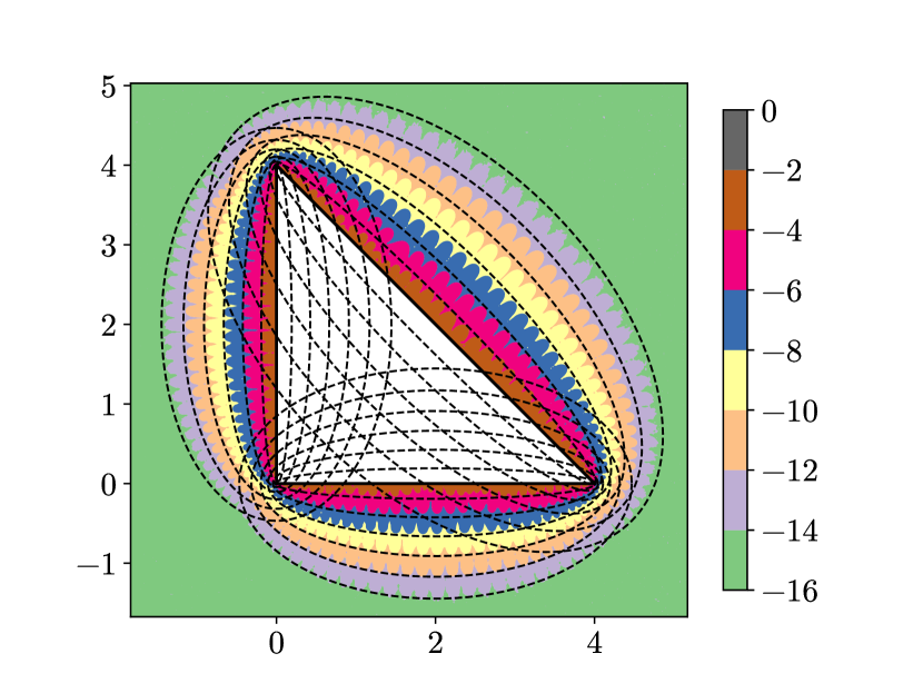
(a)

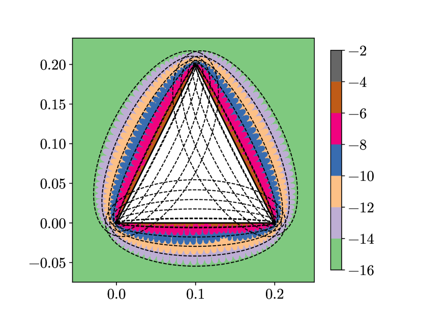
(b)

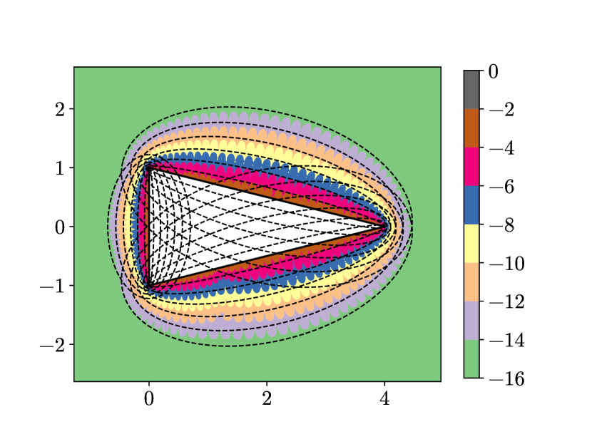
(c)

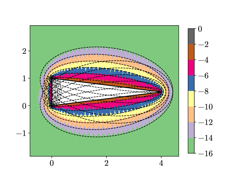
(d)

Figure 6: The contour plot of $\log_{10}E_{abs}$ with the Xiao-Gimbutas quadrature rule of order 40, and the estimation of the near field. We select the density $f$ to be $1$, and the parameter $C_{N}$ to be $2$ in all these plots.

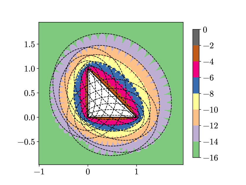
(a)

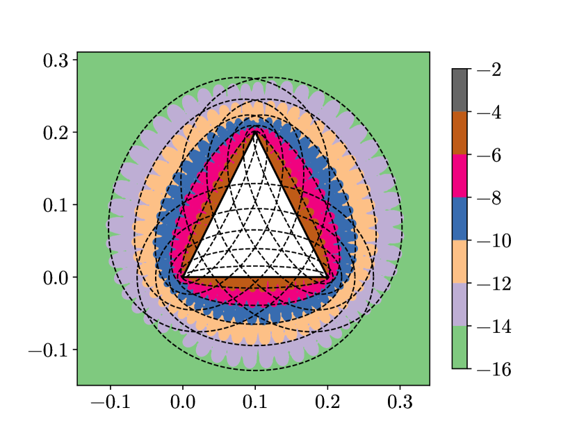
(b)

Figure 7: The contour plot of $\log_{10}E_{abs}$ with the Xiao-Gimbutas quadrature rule of order 20, and the estimation of the near field. We select the density $f$ to be $1$, and the parameter $C_{N}$ to be $6.8$ in all these plots. One can observe that when the error tolerance is low (say, $E_{abs}<10^{-14}$), the true near field is almost a ball.

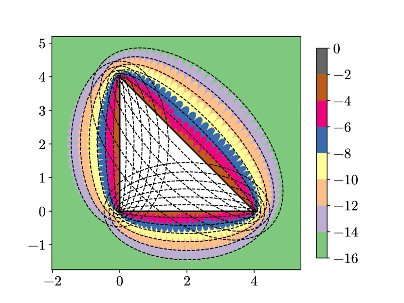
(a) $f(x,y)=\sin(x+2y)$

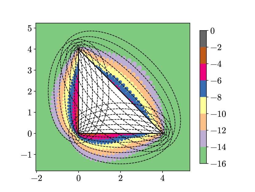
(b) $f(x,y)=\exp(-x^{2}-y^{2})$

Figure 8: The contour plot of $\log_{10}E_{abs}$ with the Xiao-Gimbutas quadrature rule of order 40, and the estimation of the near field. We select the parameter $C_{N}$ to be $2$ in all these plots. Comparing Figure 8(a) with Figure 6(a), one can observe that the near field only becomes slightly larger when the density function changes from $1$ to $\sin(x+2y)$. In general, as long as the density function can be well-resolved by the selected quadrature rule, the shape of the near field is nearly the same as the shape of the near field with density function $1$. In Figure 8(b), one can observe that the actual near field is much smaller than the predicted near field, especially for the region that is away from the origin $(0,0)$. This is because the density function $\exp(-x^{2}-y^{2})$ decays exponentially as $|x|,|y|$ increase, which cancels out the logarithmic singularity that is away from the origin. Thus, such a behavior is expected.

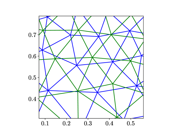
Figure 9: The staggered mesh under a microscope.

$h_{0}$	$N_{\textit{tri}}$	$N_{\textit{tot}}$
0.2	143	33033
0.1	657	151767
0.05	2766	638946

Table 4: The total number of mesh elements for different mesh sizes $h_{0}$ with $N_{s}=20$. We also report the order of the Vioreanu-Rokhlin rules, and the total number of the discretization nodes.

$\varepsilon$	$c^{0}$	$c^{+}$	$c^{*}$	$c^{*}/c^{0}$	$s_{n}^{0}$	$s_{n}^{+}$	$s_{n}^{*}$	$s_{n}^{*}/s_{n}^{0}$	$E_{\textit{abs}}^{*}$
$10^{-8}$	1.46	0.99	0.50	33.9%	15.7	9.67	4.19	26.8%	2.06$\times 10^{-8}$
$10^{-10}$	2.32	1.49	0.91	39.2%	30.7	20.2	10.3	33.7%	1.78$\times 10^{-10}$
$10^{-12}$	2.94	2.03	1.39	47.3%	55.0	36.9	22.4	40.8%	1.61$\times 10^{-12}$
$10^{-14}$	3.49	2.64	1.98	56.5%	103	72.1	47.1	45.3%	2.47$\times 10^{-14}$

Table 5: The average number of near field potential corrections, and the average number of subtriangles that need to be integrated over to resolve the nearly-singular integrand during the computation of near field interactions, for each target, with and without the precise near field analysis and the use of a staggered mesh. Note that we fine-tuned the parameters, such that $E_{\textit{abs}}^{0}$ and $E_{\textit{abs}}^{+}$ are around the same size as $E_{\textit{abs}}^{*}$.

$h_{0}$	$s_{l}^{0}$	$s_{l}^{*}$	$s_{l}^{*}/s_{l}^{0}$
$0.2$	18.8	16.5	87.6%
$0.1$	18.8	16.2	86.1%
$0.05$	18.7	16.0	85.7%

Table 6: Average number of self-interaction subdivisions with and without the use of a staggered mesh. One can observe that the use of a staggered mesh reduces the amount of computation of the self-interactions by $15\%$.

In fact, the use of the near field geometry analysis together with a staggered mesh is more powerful than Table 5 indicates, for the following reason. To make a fair comparison with the standard way of computing the near interactions (i.e., using the Vioreanu-Rokhlin rule over a single mesh), we are bound to a fixed pair of quadrature and interpolation orders. Comparing Figure 6 with Figure 7, it is easy to see that the experimental results in Table 5 will be even more impressive if we use a higher-order quadrature rule. We exploit this fact in Sections 5.1.2 and 5.2.

5.1.2 Trade-off between the far and near field interaction computations

In this section, we demonstrate the effectiveness of the offloading technique for reducing the total amount of time spent on the near field interaction computations in Figure 10. In our examples, we consider the computation of

$$u(x)=\iint_{\Omega}\frac{1}{2\pi}\log({\lVert x-y\rVert})f(y)\,\mathrm{d}A_{y},$$ (72)

where the integration domain $\Omega$ is a circle with radius $1$, and the density $f$ is

$$f(x_{0},y_{0})= \,4e^{-(x_{0}+1.6)^{2}-(y_{0}+0.2)^{2}}\cdot(x_{0}^{2}+y_{0}^{2}+3.2x_{0}+0.4y_{0}+1.6)+$$

$$\,4e^{-(x_{0}-0.2)^{2}-(y_{0}-1)^{2}}\cdot(x_{0}^{2}+y_{0}^{2}-0.4x_{0}-2y_{0}+0.04).$$ (73)

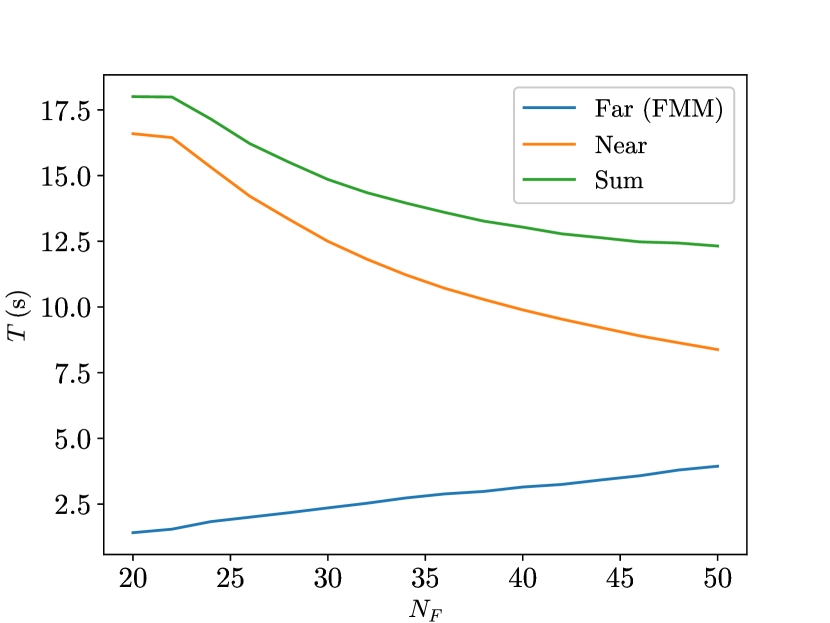
(a) $\varepsilon=10^{-14},N_{s}=20$

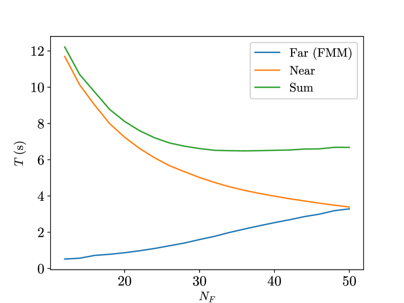
(b) $\varepsilon=10^{-14},N_{s}=12$

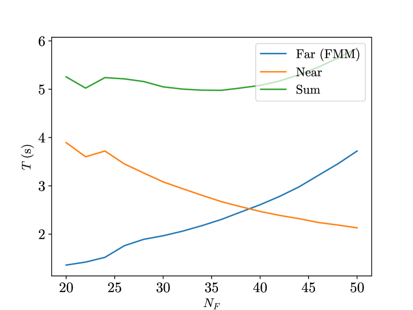
(c) $\varepsilon=10^{-10},N_{s}=20$

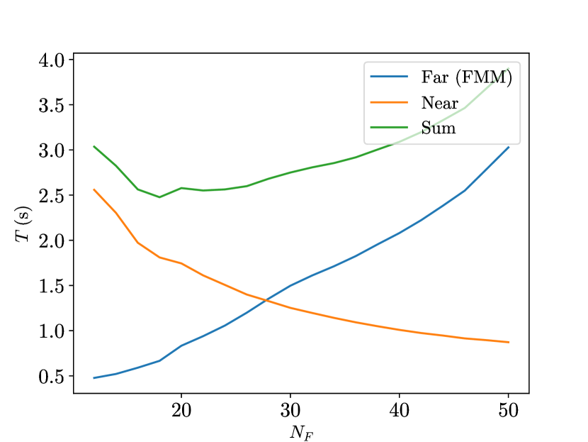
(d) $\varepsilon=10^{-10},N_{s}=12$

Figure 10: The offloading technique applied to volume potential evaluations with different interpolation orders and error tolerances, without parallelization. We fix the element size to be $h_{0}=0.1$ in all cases. If the FMM computations are parallelized, the time spent on the computation of far field interactions can be reduced dramatically, depending on the number of cores.

5.2 Computation of the volume potential and Poisson’s equation

In this section, we report the accuracy (implicitly, by reporting the accuracy of the solution to Poisson’s equation) and speed of the computation of the volume potential

$$u(x)=\iint_{\Omega}\frac{1}{2\pi}\log({\lVert x-y\rVert})f(y)\,\mathrm{d}A_{y},$$ (74)

where the density function

$$f(x_{0},y_{0})= \,4e^{-(x_{0}+1.6)^{2}-(y_{0}+0.2)^{2}}\cdot(x_{0}^{2}+y_{0}^{2}+3.2x_{0}+0.4y_{0}+1.6)+$$

$$\,4e^{-(x_{0}-0.2)^{2}-(y_{0}-1)^{2}}\cdot(x_{0}^{2}+y_{0}^{2}-0.4x_{0}-2y_{0}+0.04),$$ (75)

and the domain $\Omega$ is a wobbly ellipse, as is displayed in Figure 11. The sizes of the our experiments are presented in Table 7. We compare the performance of the algorithm, with and without the use of precise near field geometry analysis and a staggered mesh, in Tables 8 and 9. Additionally, we solve the Poisson’s equation

$$\nabla^{2}\varphi= \,f(x_{0},y_{0})\text{ in }\Omega,$$

$$\varphi= \,g(x_{0},y_{0})\text{ on }\partial\Omega,$$ (76)

where

$$g(x_{0},y_{0})=\exp(-(x_{0}+1.6)^{2}-(y_{0}+0.2)^{2})+\exp(-(x_{0}-0.2)^{2}-(y_{0}-1)^{2}),$$ (77)

and we present the error heat map in Figure 12. Below, we sketch the algorithm for solving Poisson’s equation with the use of the volume potential.

Since the volume potential

$$u(x)=\frac{1}{2\pi}\iint_{\Omega}\log{\lVert x-y\rVert}f(y)\,\mathrm{d}A_{y}$$ (78)

satisfies

$$\nabla^{2}u=f\text{ in }\Omega,$$ (79)

provided that $u^{h}:\Omega\to\mathbbm{R}$ solves Laplace’s equation

$$\nabla^{2}u^{h}=0\text{ in }\Omega,$$

$$u^{h}=g-u\text{ on }\partial\Omega,$$ (80)

we have that $\varphi:=u^{h}+u$ satisfies the given Poisson’s equation. In our implementation, we compute $u(x)|_{\partial\Omega}$ through interpolation (see Remark 3.11), from which it follows that the condition number of the interpolation matrix affects the accuracy of our computational results (see [26, 12]). Then, we find the solution to the Laplace equation (80) by the boundary integral equation method [23]. Finally, we note that the true solution $\varphi$ to this Poisson’s equation equals $g$.

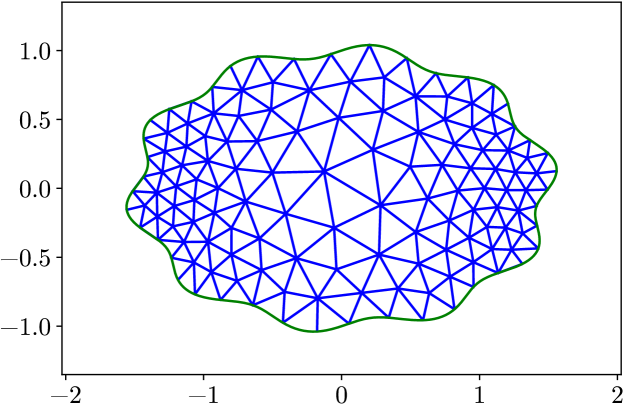
Figure 11: The wobbly ellipse domain $\Omega$ discretized by an unstructured mesh with $h_{0}=0.2$.

$h_{0}$	$N_{\textit{tri}}^{\textit{quad}}$	$N_{\textit{tri}}^{\textit{interp}}$	$N_{\textit{tot}}^{\textit{quad}}$	$N_{\textit{tot}}^{\textit{interp}}$
0.2	231	225	102564	51975
0.1	1001	997	444444	230307
0.05	4183	4172	1857252	963732

Table 7: The total number of mesh elements, quadrature and interpolation nodes for different mesh sizes $h_{0}$. In this table, we set $N_{f}=50,N_{s}=20$.

$\varepsilon$	$h_{0}$	$T_{\mathcal{F}+\mathcal{N}}^{0}$	$T_{\mathcal{F}+\mathcal{N}}^{*}$	$\frac{T_{\mathcal{F}+\mathcal{N}}^{*}}{T_{\mathcal{F}+\mathcal{N}}^{0}}$	$T_{\mathcal{S}}^{0}$	$T_{\mathcal{S}}^{*}$	$T_{\textit{tot}}^{0}$	$T_{\textit{tot}}^{*}$	$\widetilde{E}_{\textit{abs}}^{*}$	$\frac{\#\textit{tgt}}{\textit{sec}}$
$10^{-10}$	$0.2$	4.14	1.98	47.8%	2.64	2.39	7.08	4.72	2.66$\times 10^{-9}$	1.10$\times 10^{4}$
	$0.1$	16.0	7.93	49.4%	12.3	11.0	30.3	21.0	2.42$\times 10^{-9}$	1.10$\times 10^{4}$
	$0.05$	60.5	29.6	49.0%	50.9	45.3	85.9	46.9	4.69$\times 10^{-9}$	1.12$\times 10^{4}$
$10^{-14}$	$0.2$	9.69	5.96	61.5%	2.65	2.72	12.6	9.06	2.42$\times 10^{-12}$	5.73$\times 10^{3}$
	$0.1$	36.3	19.3	53.2%	12.5	11.4	50.6	32.7	4.13$\times 10^{-13}$	7.05$\times 10^{3}$
	$0.05$	136	67.2	49.3%	70.7	63.4	217	141	4.54$\times 10^{-13}$	6.84$\times 10^{3}$

Table 8: Comparisons of the computational time of the volume potential evaluation with $20$th order interpolation of the solution, without parallelization. When $\varepsilon=10^{-10}$, we set $N_{f}=40$, $N_{n}=12$, $N_{l}=10$, $N_{g}=8$; when $\varepsilon=10^{-14}$, we set $N_{f}=50$, $N_{n}=12$, $N_{l}=10$ (except that $N_{l}=14$ when $h_{0}=0.05$), $N_{g}=8$. In all of these experiments, the Vioreanu-Rokhlin rule of order $20$ is used in the naive case indicated by the superscript $0$. It is important to note that we only report the error of the approximation to the solution to Poisson’s equation here, as the analytic solution for the volume potential is not available. However, we note that the actual accuracy of the volume potential evaluations is higher than the one shown in the $\widetilde{E}_{abs}^{*}$ column, due to the use of not perfectly-conditioned interpolation matrices. Note that we fine-tuned the parameters, such that $E_{\textit{abs}}^{0}$ is around the same size as $E_{\textit{abs}}^{*}$.

$\varepsilon$	$h_{0}$	$T_{\mathcal{F}}^{0}$	$T_{\mathcal{F}}^{*}$	$T_{\mathcal{N}}^{0}$	$T_{\mathcal{N}}^{*}$	$\frac{T_{\mathcal{N}}^{*}}{T_{\mathcal{N}}^{0}}$
$10^{-10}$	$0.2$	0.55	0.84	3.59	1.15	31.9%
	$0.1$	2.75	4.10	13.3	3.83	28.8%
	$0.05$	11.7	17.3	48.8	12.3	25.2%
$10^{-14}$	$0.2$	0.63	1.47	9.07	4.49	49.5%
	$0.1$	3.15	6.39	33.1	12.9	39.0%
	$0.05$	13.3	27.0	123	40.2	32.6%

Table 9: Comparisons of the computational time of the far and near field interactions with $20$th order interpolation of the solution, without parallelization. The setting of the experiments shown in this table is the same as the ones shown in Table 8. It is important to note that, when one parallelizes the FMM computations, $T_{\mathcal{F}}$ becomes negligible as the number of cores increases, from which it follows that the computational time, with the use of near field geometry analysis and a staggered mesh, is roughly equal to the values in the $\frac{T_{\mathcal{N}}^{*}}{T_{\mathcal{N}}^{0}}$ column times the naive computational time.

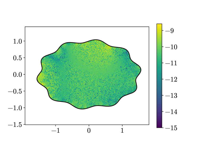
(a) $\varepsilon=10^{-10}$

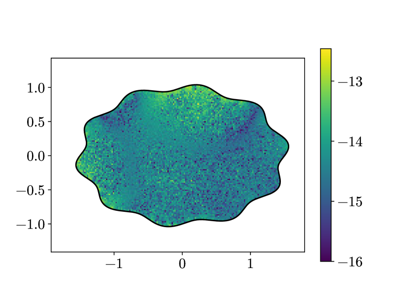
(b) $\varepsilon=10^{-14}$

Figure 12: The heat maps of $\log_{10}\widetilde{E}_{abs}$ when $h_{0}=0.05$. The results are computed by evaluating the interpolants.

6 Conclusions and further directions

In this paper, we present three complementary techniques for accelerating potential calculations over unstructured meshes, as well as a robust and extensible framework for the evaluation and interpolation of 2-D volume potentials over complicated geometries. With the use of precise near field geometry analysis, we show that one can eliminate all of the unnecessary near field potential computations. By introducing the use of a staggered mesh, we further show that the number of interpolation nodes at which the near field and self-interactions are costly to evaluate is reduced dramatically. These two observations facilitate the offloading technique, which transforms the expensive and unstructured near field interaction computation into the highly-optimized parallel FMM computation. Of the methods described in this paper, we believe the offloading technique to be the most general, since we expect that the near field will become vanishingly small when the order of the far field quadrature rule is high, for other kernels, geometries and in higher dimensions. The offloading technique is one of the few methods we are aware of for which the use of extremely high-order quadrature rules is essential.

In the following sections, we discuss the generalizations and extensions of the techniques and the volume potential evaluation algorithm presented in this paper.

6.1 Precise near field geometry analysis for different kernels and domains

Although the near field geometry analysis is only applied to the 2-D Newtonian potential in this paper, the same analysis can be trivially generalized to the 2-D Helmholtz volume potential, as its kernel has the same type of logarithmic singularity. The same approach to analyzing the near field can be applied to, for example, quadrilateral elements in 2-D, and more complicated elements in 3-D, although we expect the near field geometry analysis in 3-D to be substantially more involved.

Since surfaces are often represented by a collection of mappings from 2-D domains, and surfaces are often discretized by meshing these 2-D domains using unstructured meshes, the generalization of the near field geometry analysis to the on-surface evaluation of surface potentials is similar to the near field analysis presented in this paper, except that the kernel becomes more singular, and the effect of the mapping on the near field must be accounted for.

6.2 The offloading technique for computing surface and 3-D volume potentials

The offloading technique clearly can be generalized to the computation of surface and 3-D volume potentials, provided that high-order quadrature rules are available. In practice, high-order quadrature rules for tetrahedra or cubes are presently not available. For example, the highest order quadrature rule for tetrahedra reported in [28] is 15, which is far from enough for the offloading technique to be effective.

6.3 The staggered mesh for surfaces and 3-D volumes

Our heuristic way of generating the staggered mesh, described in Section 4.3, can be trivially generalized to the surface mesh and 3-D volume mesh case. Furthermore, the use of a staggered mesh can similarly accelerate the potential interpolation in these cases.

6.4 Accelerating near and self-interaction computations by specialized quadrature rules

Our focus in this paper is to accelerate the far and near field interaction computations. The self-interaction computations are minimally optimized. After applying all of the optimizations proposed in this paper, one can observe from Table 8 that the self-interaction evaluation cost becomes a bottleneck of the algorithm. As is noted in Remark 3.9, this cost can be reduced dramatically by precomputing a large number of specialized quadrature rules.

In the computation of near field interactions, we use the most naive scheme, i.e., adaptive subdivision, for resolving the nearly-singular integrand, and we anticipate that the cost can be further reduced with the use of more advanced methods (see, for example, [1]). The techniques proposed in this paper are compatible with other schemes for the computation of near field and self-interactions.

7 Acknowledgements

We sincerely thank James Bremer for his helpful advice and for our informative conversations.

Appendix A Appendix: Geometric algorithms

In this appendix, we provide a description of all of the geometry processing algorithms used in this paper.

A.1 Quadtree

A quadtree is a tree data structure used to efficiently store points in a two-dimensional space. More specifically, it partitions the domain into boxes by recursively subdividing each box into four sub-boxes until each leaf box contains no more than $m$ points, where $m$ is a user-specified number. Given a set of $n$ points that are uniformly distributed, it takes $\mathcal{O}(n\log n)$ operations to construct a quadtree for these points. After the quadtree is constructed, it takes $\mathcal{O}(\log n)$ operations to find all of the leaf boxes that intersect a given rectangle. We refer readers to Chapter 37 of [21] for a detailed introduction to the quadtree data structure.

A.2 Construction of a signed distance function from a set of parametrized curves

In this section, we first introduce the concept of signed distance function (SDF), and then describe an efficient algorithm for computing the SDF of a geometry with boundaries described by a set of closed curves

$$\bigl{\{}\gamma_{i}(s)\bigr{\}}_{i},\,\,\gamma_{i}:[0,L_{i}]\to\mathbbm{R}^{2},\,\,i=1,2,\dots,N,$$ (81)

where $\gamma_{i}$ is a unit-speed parameterization, and $L_{i}$ is the total arc length of $\gamma_{i}$. Below, we give the formal definition of a signed distance function.

Definition A.1 (Signed distance function).

Given a geometry $\Omega$ with boundaries described by a set of closed curves $\{\gamma_{i}(s)\}$, the signed distance function $h:\mathbbm{R}^{2}\to\mathbbm{R}$ determines the distance of a given point $x$ from the boundary of $\Omega$, with the sign indicates whether $x$ is inside $\Omega$ or not. By convention, $h(x)$ is positive for $x\in\Omega$, and negative for $x\in\Omega^{c}$.

Our algorithm for converting the parameterized boundary curves into an SDF is outlined as follows. We begin with the following precomputation:

1. (Sampling) Generate equidistant sampling points over the boundaries, where the number of total sampling points depends on the required accuracy. In addition, we store the corresponding curve parameter for each sampling point.

2. (Quadtree) Create a quadtree data structure for the sampling points (see Appendix A.1).

Then, we evaluate the signed distance function at any given target location $x$ by the following steps.

1. Create a rectangle centered at $x$ with appropriate side lengths.

2. Query all of the sampling points that are inside the rectangle by exploiting the quadtree data structure. If no points are captured by the rectangle, increase the size of the rectangle and perform the query step again.

3. Loop through all of the captured sampling points, and find the point $x^{\prime}$ that is closest to the target point $x$.

4. (Optional) Do a few iterations of Newton’s method using $x^{\prime}$ as the initial guess to get a highly accurate approximation to the closest point on the boundaries.

5. Return $\mathop{\mathrm{sgn}}({\langle x^{\prime}-x,n_{x^{\prime}}\rangle}){\lVert x^{\prime}-x\rVert}$ as the SDF value at $x$, where $n_{x^{\prime}}$ denotes the outward-pointing normal vector of the boundary at $x^{\prime}$, and $\mathop{\mathrm{sgn}}(\cdot)$ represents the sign function.

Remark A.1.

The necessity of Newton’s method in this algorithm depends on the accuracy needed for the SDF evaluation. Without the use of Newton’s method, the accuracy is proportional to $h$, where $h$ is the spacing of the equidistant sampling points.

Remark A.2.

One can also construct a signed distance function from a domain represented as an implicit function (see Section 4 in [24]).

A.3 Distmesh

Distmesh [24] is a simple and short algorithm for generating a triangle mesh for a geometry with boundaries described by a signed distance function. The algorithm is based on the physical analogy between a simplex mesh and a truss structure, and the triangle mesh is computed by solving an ordinary differential equation for the equilibrium in the truss structure composed of compressible springs (using piecewise linear force-displacement relations). Despite its simplicity, the generated triangles are of high quality, in the sense that most of the triangles are close to equilateral, which is important in many applications.

Below, we describe the Distmesh algorithm briefly (see [24] for details).

1. (Initial guess) Create an initial node distribution arranged in a triangular tiling inside a bounding box of the input geometry, and remove the nodes outside the geometry.

2. (Reset topology) Compute a triangle mesh by applying the Delauney triangulation algorithm to the nodes.

3. (Compute equilibrium) Solve for the equilibrium in the truss structure represented by the triangle mesh using the forward Euler method. When some nodes end up outside the geometry, move them back to the closest point on the boundary, where the closest point is computed using the SDF.

4. Go back to Step 2 when the total movements of nodes in Step 3 become large. Otherwise, return the final triangle mesh.

Observation A.3.

It is often desirable to resolve a complex geometry by adaptive meshing, i.e., requiring mesh elements close to a singularity to be smaller relative to elements further away. This can be achieved using Distmesh by setting the equilibrium lengths of the springs (by analogy with a truss system) near the singularities to be shorter than the equilibrium length of the rest of the springs. In practice, the desired equilibrium lengths of the springs are specified by a so-called element size function (see [24] and Observation A.5 for details).

Observation A.4.

The quality of a mesh generated by the Distmesh algorithm is relatively insensitive to the computational accuracy of the solution to the evolution equations of the truss system, and to the computational accuracy of the SDF evaluation. Therefore, the use of the forward Euler method, whose order of convergence is one, is sufficient for our purpose. For the same reason, when the SDF is computed using the algorithm described in Appendix A.2, it is unnecessary to use Newton’s method to improve its accuracy.

A.4 Modified Distmesh algorithm for constructing a curved triangulation

In Appendix A.3, we describe a simple triangle mesh generation algorithm named Distmesh, introduced in [24]. To apply Distmesh to our particular problem, several additional pieces of information must be returned by the algorithm, including:

• Given a mesh element, whether it is a triangle or a curved element;

• Given a curved element, which vertex is opposite to that curved side;

• The curve parameters that correspond to the endpoints of a curved side.

These issues can be remedied with several modifications to the Distmesh algorithm. In addition, we present a simple technique for improving the triangle mesh quality using the new outputs.

Firstly, given a triangle mesh, based on the observation that the boundary edges are the edges that are associated only with a single element, it is easy to quickly identify all of the boundary edges, boundary vertices and curved elements (including the vertices opposite to the curved sides). In addition, we also observe that the use of the signed distance function (described in Appendix A.2) allows us to quickly determine the curve parameters corresponding to the endpoints of a curved side. So far, all of the required information stated above can be computed for any given triangle mesh and its associated boundary.

The mesh quality can be improved by the following modification. During the computation of the equilibrium state of the truss structure, as noted in Appendix A.3, some nodes, especially the ones that are located on the boundary, may end up outside the geometry. The original Distmesh algorithm handles this by projecting each outside node to the closest point on the boundary at the end of each iteration. In other words, when solving for the equilibrium, the boundary is neglected until the very end of each iteration. Such treatment is somehow non-physical, since the boundary should be treated as a hard obstacle at all stages. Therefore, in our implementation, we maintain an array of flags that indicates whether or not a node is on the boundary, and ensure that for every boundary node, the force component that is normal to the boundary is eliminated. This way, only forces tangential to the boundary can contribute to the computation. Although some nodes will still end up outside the geometry and require projection back to the closest point on the boundary at the end of each iteration, their movements become more physical, and it improves the triangle mesh quality.

Finally, we note that such modification is impossible without keeping track of the boundary nodes.

Observation A.5.

Recall that Distmesh uses an element size function to control the sizes of mesh elements (see Observation A.3). We find the element size function

$$h(x,y):=\oint_{\partial\Omega}e^{-a((x-x_{0})^{2}+(y-y_{0})^{2})}\cdot\kappa(x_{0},y_{0})\,\mathrm{d}s$$ (82)

gives a mesh that resolves the boundary of the domain well (see Figure 11), where $\kappa(x_{0},y_{0})$ denotes the curvature of $\partial\Omega$ at $(x_{0},y_{0})$, and $a$ is a constant that depends on the scale of the domain and the size of the mesh elements.

Remark A.6.

In fact, the volume potential evaluation algorithm of the paper does not depend on any particular meshing algorithm. All that is needed is a triangle mesh of good quality which contains all of the required information described in this section.

A.5 Nearby mesh elements query

Due to the singularity of the Green’s function, it is important to identify all nearby mesh elements at a given target location, so that the elements close to or containing the target can be handled separately from the mesh elements that are far away. In this section, we introduce an algorithm for finding all of the mesh elements that are within a certain distance of a given target $x$, together with the particular element that $x$ lies within (if such an element exist). The procedure is outlined as follows. We first preprocess the triangle mesh:

1. (Sampling) For each mesh element, sample the four vertices of its bounding box. Associate each sampling point with the index of the mesh element that it is sampled from.

2. (Quadtree) Create a quadtree data structure for the sampling points (see Appendix A.1).

Then, we find the nearby mesh elements of a given target $x$. Formally speaking, given a query box centered at $x$ of size larger than the sizes of the bounding boxes of adjacent mesh elements of the target, we find all of the elements that intersect the query box, as follows.

1. Find all the sampling points that are inside the query box by exploiting the quadtree data structure.

2. Return the associated element indices of the captured sampling points.

Finally, we are also able to find the particular mesh element that $x$ lies within (if any):

1. (Optional) Evaluate the signed distance function (see Appendix A.2) at $x$, and return null if $x$ is outside the domain $\Omega$.

2. Loop through all of the nearby elements of $x$ (obtained through the previous computation). For each element:

   • If the element is a triangle, return the index if the barycentric coordinates of $x$ with respect to the element are all between zero and one;

   • If the element is a curved element (denoting the vertex opposite to the curved side by $O$), return the index if both of the following conditions are satisfied:

     • The polar angle of $x$ is in between the polar angles of the two straight sides of the curved element, with respect to polar coordinates centered at $O$.

     • The distance between $x$ and $O$ is smaller than the distance between $x^{\prime}$ and $O$, where $x^{\prime}$ denotes the point at which the line $x^{\prime}O$ and the curved side intersects.

As is stated in our assumption above, it is important to have the query box be larger than the sizes of the bounding boxes of adjacent mesh elements of the target location, since otherwise, the query box can overlap with the bounding box without capturing any of its vertices, which leads to uncaptured nearby elements (see Figure 13).

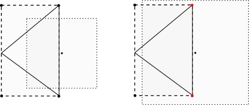
Figure 13: The size of the query box has to be larger than its nearby bounding boxes. On the left, the triangle is not captured by the query box, as the size of the box is too small. This can be fixed by increasing the size of the box, as is shown on the right.

Remark A.7.

The construction of the quadtree above takes $\mathcal{O}(n\log n)$ operations, and the use of the quadtree to query nearby elements takes $\mathcal{O}(\log n+m)$ operations, where $n$ and $m$ are the total number of mesh elements and nearby elements, respectively (see Appendix A.1). We note that in practice, $m=\mathcal{O}(1)$.

Remark A.8.

This query algorithm can be easily generalized to meshes of other types, e.g., the quadrilateral mesh.

References

- [1] T. G. Anderson, H. Zhu, and S. Veerapaneni, A Fast, High-Order Scheme for Evaluating Volume Potentials on Complex 2D Geometries via Area-to-Line Integral Conversion and Domain Mappings, arXiv:2203.05933v1, 2022.
- [2] M. Anita, The Rapid Evaluation of Volume Integrals of Potential Theory on General Regions, J. Comput. Phys., 100.2 (1992), pp. 236–245.
- [3] T. Askham, and A. J. Cerfon, An Adaptive Fast Multipole Accelerated Poisson Solver for Complex Geometries, J. Comput. Phys., 344 (2017), pp. 1–22.
- [4] A. H. Barnett, Evaluation of Layer Potentials Close to the Boundary for Laplace and Helmholtz Problems on Analytic Planar Domains, SIAM J. Sci. Comput., 36.2 (2014), pp. A427–451.
- [5] D. Braess, Nonlinear Approximation Theory. Vol. 7. Springer Science & Business Media, 2012.
- [6] J. Bremer, and Z. Gimbutas, A Nyström Method for Weakly Singular Integral Operators on Surfaces, J. Comput. Phys., 231.14 (2012), pp. 4885–4903.
- [7] J. Bremer, and Z. Gimbutas, On the Numerical Evaluation of the Singular Integrals of Scattering Theory, J. Comput. Phys., 251 (2013), pp. 327–343.
- [8] J. Bremer, Z. Gimbutas, and V. Rokhlin, A Nonlinear Optimization Procedure for Generalized Gaussian Quadratures, SIAM J. Sci. Comput., 32.4 (2010), pp. 1761–1788.
- [9] F. Ethridge, and L. Greengard, A New Fast-Multipole Accelerated Poisson Solver in Two Dimensions, SIAM J. Sci. Comput., 23.3 (2001), pp. 741–760.
- [10] J. Garritano, Y. Kluger, V. Rokhlin, and K. Serkh, On the Efficient Evaluation of the Azimuthal Fourier Components of the Green’s Function for Helmholtz’s Equation in Cylindrical Coordinates, arXiv:2104.12241, 2021.
- [11] Z. Gimbutas, and L. Greengard, Computational Software: Simple FMM Libraries for Electrostatics, Slow Viscous Flow, and Frequency-Domain Wave Propagation, Commun. Comput. Phys., 18.2 (2015), pp. 516–528.
- [12] Z. Gimbutas, and H. Xiao, Quadratures for triangles, squares, cubes and tetrahedra, https://github.com/zgimbutas/triasymq, 2020.
- [13] W. J. Gordon, and C. A. Hall, Construction of Curvilinear Co-Ordinate Systems and Applications to Mesh Generation, Int. J. Numer. Methods Eng., 7.4 (1973), pp. 461–477.
- [14] W. J. Gordon, and C. A. Hall, Transfinite Element Methods: Blending-Function Interpolation over Arbitrary Curved Element Domains, Numer. Math., 21.2 (1973), pp. 109–129.
- [15] L. Greengard, and V. Rokhlin, A Fast Algorithm for Particle Simulations, J. Comput. Phys., 135.2 (1997), pp. 280–292.
- [16] L. Greengard, M. O’Neil, M. Rachh, and F. Vico, Fast Multipole Methods for the Evaluation of Layer Potentials with Locally-Corrected Quadratures, J. Comput. Phys.: X, 10 (2021), pp. 100092.
- [17] L. af Klinteberg, and A. K. Tornberg, Adaptive Quadrature by Expansion for Layer Potential Evaluation in Two Dimensions, SIAM J. Sci. Comput., 40.3 (2018), pp. A1225–1249.
- [18] L. af Klinteberg, and A. K. Tornberg, Error Estimation for Quadrature by Expansion in Layer Potential Evaluation, Adv. Comput. Math., 43.1 (2017), pp. 195–234.
- [19] L. af Klinteberg, C. Sorgentone, and A. K. Tornberg, Quadrature Error Estimates for Layer Potentials Evaluated near Curved Surfaces in Three Dimensions, Comput. Math. with Appl., 111 (2022), pp. 1–19.
- [20] T. Koornwinder, Two-variable analogues of the classical orthogonal polynomials, Theory and Application of Special Functions., R. Askey, Ed. (1975), pp. 435–495.
- [21] J. F. Hughes, A. Van Dam, M. McGuire, J. D. Foley, D. Sklar, S. K. Feiner, and K. Akeley, Computer graphics: principles and practice, Pearson Education, 2014.
- [22] D. Malhotra, and G. Biros, PVFMM: A Parallel Kernel Independent FMM for Particle and Volume Potentials, Commun. Comput. Phys., 18.3 (2015), pp. 808–830.
- [23] P. G. Martinsson, Fast Direct Solvers for Elliptic PDEs, CBMS-NSF Conference Series, vol. CB96. SIAM, Philadelphia, 2019.
- [24] P. O. Persson, and G. Strang, A Simple Mesh Generator in MATLAB, SIAM Rev., 46.2 (2004), pp. 329–345.
- [25] L. N. Trefethen, Approximation Theory and Approximation Practice. SIAM, 2019.
- [26] B. Vioreanu, and V. Rokhlin, Spectra of Multiplication Operators as a Numerical Tool, SIAM J. Sci. Comput., 36.1 (2014), pp. A267–288.
- [27] B. Williamson, An Elementary Treatise on the Differential Calculus, 9th ed. Dublin University Press, 1899.
- [28] H. Xiao, and Z. Gimbutas, A Numerical Algorithm for the Construction of Efficient Quadrature Rules in Two and Higher Dimensions, Comput. Math. with Appl., 59.2 (2010), pp. 663–676.
- [29] W. Ying, and W. C. Wang, A Kernel-Free Boundary Integral Method for Variable Coefficients Elliptic PDEs, Commun. Comput. Phys., 15.4 (2014), pp. 1108–1140.
- [30] B. Szabó, and I. Babuška, Finite element analysis, John Wiley & Sons, 1991.
- [31] R. Yokota, and L. A. Barba, A Tuned and Scalable Fast Multipole Method as a Preeminent Algorithm for Exascale Systems, Int J High Perform Comput Appl., 26.4 (2012), pp. 337–346.
- [32] H. Zhu, Fast, High-Order Accurate Integral Equation Methods and Application to PDE-Constrained Optimization, PhD thesis, University of Michigan, 2021.