Evolution of Brill waves with an adaptive pseudospectral method

Abstract

As a first application of the new adaptive mesh functionality of the the pseudospectral numerical relativity code bamps, we evolve twist-free, axisymmetric gravitational waves close to the threshold of collapse. We consider six different one-parameter families of Brill wave initial data; two centered and four off-centered families. Of these the latter have not been treated before. Within each family we tune the parameter towards the threshold of black hole formation. The results for centered data agree with earlier work. Our key results are first, that close to the threshold of collapse the global peak in the curvature appears on the symmetry axis but away from the origin, indicating that in the limit they will collapse around disjoint centers. This is confirmed in three of the six families by explicitly finding apparent horizons around these large curvature peaks. Second, we find evidence neither for strict discrete-self-similarity nor for universal power-law scaling of curvature quantities. Finally, as in Ledvinka & Khirnov’s recent study, we find approximately universal strong curvature features. These features appear multiple times within individual spacetimes close to the threshold and are furthermore present within all six families.

I Introduction

Working in spherical symmetry with a massless scalar field minimally coupled to the Einstein field equations, and tuning in solution space to the verge of black hole formation, Choptuik [1] observed behavior with a striking resemblance to that observed near critical points in other areas of physics. For instance, near a thermodynamic critical point, as the correlation length diverges the system is rendered scale invariant. Order parameters then follow power-laws with universal critical exponents. Universality, power-law behavior, and scale invariance (also called self-similarity) are together referred to as critical phenomena. The discovery of all three in gravitational collapse are thus known as critical phenomena in gravitational collapse.

Despite the familiarity of the phenomena, what is meant as the critical point in gravitational collapse has its own particular definition. The threshold of collapse can be conveniently identified by considering families of initial data labeled by a single-parameter $p$. The parameter varying within a family is conventionally chosen such that for small values of the parameter ($p<p_{\star}$), the field content will eventually disperse and lead asymptotically to flat space. On the other hand large values of the parameter ($p>p_{\star}$), lead to black hole formation and thus the presence of a singularity of some description. Of deep interest is the threshold of collapse $p=p_{\star}$. Within the analogy to statistical physics, the critical point is precisely the threshold of collapse.

The manifestation of critical phenomena in gravitational collapse have their own specifics. Regarding for instance scale-invariance, by using a suitable time coordinate close to the threshold of collapse, Choptuik observed progressively scaled down, periodic repetitions of a field configuration that appeared independently of the family under consideration. Closer to the threshold more and more of these echoes were found. This lead to the conjecture that around the center of collapse, the threshold spacetime within any family agrees with that of any other, and that this limiting spacetime itself is discretely self-similar (DSS). The limiting spacetime is therefore referred to as the critical solution or Choptuik spacetime. Such a spacetime has been proven to exist [2]. Universality was also observed in the periodicity of these echoes, as well as in the exponent, $\gamma$, of the power-law that the masses of near critical black holes obey,

$$M_{\text{BH}}\simeq|p-p_{\star}|^{\gamma}.$$ (1)

In [3], it was argued on dimensional grounds and confirmed empirically that below the threshold an analogous scaling relation should hold for the spacetime maximum of curvature scalars such as the Kretschmann scalar $I=R_{abcd}{}R^{abcd}$, so that

$$I_{\text{max}}{}^{-1/4}\simeq|p-p_{\star}|^{\gamma}.$$ (2)

Arguments of [4, 5] suggest that if the critical spacetime is DSS then this power-law should occur with a periodic wiggle superimposed. The above properties have been repeatedly verified for the spherical massless scalar field for many different families of data. In spherical symmetry various alternative matter models have been considered and, although details such as the values of the power-law parameters or the specific type of self-similarity differ, the basic ingredients persist (see the canonical review [6] for details).

Less clear is the precise extent to which critical phenomena extend beyond spherical symmetry. In line with the conjecture that there is a single strong-field solution lying between dispersion and collapse, for the original matter model of a massless scalar field it is known [7] that nonspherical linear mode perturbations about the critical solution decay. On the other hand nonlinear numerical work in axisymmetry [8, 9], which is much more challenging than the spherical setting, indicates that both power-law behavior and periodicity vary in the presence of increasing aspherical perturbations, and furthermore that the single center of collapse generically splits into two distinct centers resembling to an extent the Choptuik spacetime. There are even a small number of studies in full-3d [10, 11], which are again correspondingly more numerically challenging and thus remain further from the threshold. Keeping the axisymmetric setup but considering electromagnetic waves [12, 13] as a matter model has proven to show the exact same difficulty in establishing strict DSS and universal critical exponents, and again the appearance of multiple centers of collapse. Evolutions of complex scalar field content with angular momentum also suggests a more complicated structure in phase space [8]. Toy models [14] also suggest that universality could be more subtle as one moves away from spherical symmetry and more parameters are needed to parameterize threshold solutions. These issues demand deeper investigation in axisymmetry and full-3d.

As the simplest scenario in which dynamical gravitational waves occur, the aforementioned axisymmetric setting is of special interest in general relativity (GR). By working in vacuum we can try to understand the aspect of critical collapse determined by pure gravity. Two main types of vacuum initial data have been considered: Brill and Teukolsky waves. The former were introduced by Brill [15] and refer to a solution of the constraint equations in axisymmetric vacuum at a moment of time symmetry. The latter, constructed first by Teukolsky [16], and generalized from quadrupolar to include all multipoles by Rinne [17], are general vacuum solutions to the linearized Einstein field equations in transverse-traceless gauge. For a comparison between these two types of waves at the linear level see [18]. As linearized solutions, Teukolsky wave initial data has to be dressed up to construct solutions of the constraint equations of GR. There are several strategies to do so [19, 20, 21, 22, 23, 24].

Concerning vacuum time evolutions, Abrahams and Evans [19, 20] were the first to study gravitational waves near the threshold of collapse already in the early 1990s. Following the basic approach of Choptuik they evolved members of one-parameter families of (constraint solved) Teukolsky waves without moment of time symmetry and tuned to the threshold. They observed echoes and found that for supercritical data the black hole masses also obey the power-law (1). Since then, numerous authors, [25, 26, 27, 28, 29, 24, 30, 31, 32] have evolved gravitational waves to investigate the threshold of collapse, but none have unambiguously recovered this early success. Two of these deserve special attention here. First, in [30], the direct precursor to the present work, a single family of Brill waves was considered. In qualitative agreement with other axisymmetric simulations [8, 9, 12, 13], close to the threshold global maxima of the curvature form away from the origin as the consequence of large spikes appearing in the curvature. In collapse spacetimes, a disjoint pair of horizons were found along the symmetry axis around the largest of the foregoing curvature spikes. Tentative evidence for power-law scaling with a periodic wiggle was found for the Kretschmann scalar, but nothing could be concluded about universality with only one family. In important recent work, Ledvinka and Khirnov [32] directly confirmed these findings using a different gauge and completely independent code, and tuning to a comparable neighborhood of the threshold. Studying now multiple families of initial data, they furthermore found pairs of apparent horizons (AHs) also in (constraint solved) Teukolsky waves. Once more in qualitative agreement with other work in axisymmetry, they also report that although power-law scaling does appear within given families, the power itself does not seem to be universal. And there furthermore seems to be no universal threshold solution. That said, the most important finding of [32] is the presence of repeated curvature features which although not appearing in a strictly DSS fashion, do appear to be universal.

The key obstacle encountered by both [30] and [32] was in tuning $p$ to $p_{\star}$. For context, in spherical symmetry, either by using adaptive mesh refinement (AMR) as in [1] or well-chosen coordinates as in [3], it is often possible to tune to machine precision $|p-p_{\star}|\sim 10^{-15}$. In axisymmetric matter evolutions, values like $|p-p_{\star}|\sim 10^{-9}$ are often possible, whereas the best that could be managed in [30] was $|p-p_{\star}|\sim 10^{-5}$. There are several reasons for this. With less symmetry the numerical cost to reach a given level of accuracy is necessarily higher. Despite using a pseudospectral numerical method adapted to axisymmetry [33, 34], the computational cost of the evolutions skyrocketed near the threshold of collapse as finer curvature features form and more resolution is needed. For example in [30] approximately $10^{6}$ core hours were used for a single family. Besides that, it was found that near the threshold, spacetimes simply could not be classified as the evolution would fail before an AH could be found. It was unclear whether this was caused by a lack of resolution, constraint violation rendering the solution unphysical, or the formation of coordinate singularities.

Presently we return to the problem of vacuum critical collapse with our pseudospectral code bamps. To mitigate against computational cost the code has undergone a major redesign since [30], and now employs AMR. Here we present evolutions of six different families of Brill wave initial data. As was done previously, we evolved prolate and oblate centered Brill waves. We also evolved four off-center families of Brill waves that have not been treated before. The paper is structured as follows. In section II we give a brief overview of our formulation and numerical methods. Complete details of our approach to AMR will be given in a forthcoming sister paper. In section III we explain our initial data, approach to tuning and our new apparent horizon finder. Our numerics are presented in section IV, before a closing discussion in section V.

II Formulation and numerical setup

The time evolution of the different sets of initial data were performed using the bamps code. To evolve the spacetime, we use a first order reduction of the generalized harmonic gauge (GHG) formulation [35] of the Einstein equations, with gauge choices as described in [34]. The field equations are

$$\partial_{t}\tensor{g}{{}_{a}{}_{b}} =\beta^{i}\partial_{i}\tensor{g}{{}_{a}{}_{b}}-\alpha\tensor{\Pi}{{}_{a}{}_{b}}+\gamma_{1}\beta^{i}\tensor{C}{{}_{i}{}_{a}{}_{b}}$$

$$\partial_{t}\tensor{\Phi}{{}_{i}{}_{a}{}_{b}} =\beta^{j}\partial_{j}\tensor{\Phi}{{}_{i}{}_{a}{}_{b}}-\alpha\partial_{i}\tensor{\Pi}{{}_{a}{}_{b}}+\gamma_{2}\alpha\tensor{C}{{}_{i}{}_{a}{}_{b}}$$

$$\quad+\frac{1}{2}\alpha n^{c}n^{d}\tensor{\Phi}{{}_{i}{}_{c}{}_{d}}\tensor{\Pi}{{}_{a}{}_{b}}+\alpha\gamma^{jk}n^{c}\tensor{\Phi}{{}_{i}{}_{j}{}_{c}}\tensor{\Phi}{{}_{k}{}_{a}{}_{b}}$$

$$\partial_{t}\tensor{\Pi}{{}_{a}{}_{b}} =\beta^{i}\partial_{i}\tensor{\Pi}{{}_{a}{}_{b}}-\alpha\gamma^{ij}\partial_{i}\tensor{\Phi}{{}_{j}{}_{a}{}_{b}}+\gamma_{1}\gamma_{2}\beta^{i}\tensor{C}{{}_{i}{}_{a}{}_{b}}$$

$$\quad+2\alpha g^{cd}\left(\gamma^{ij}\tensor{\Phi}{{}_{i}{}_{c}{}_{a}}\tensor{\Phi}{{}_{j}{}_{d}{}_{b}}-\tensor{\Pi}{{}_{c}{}_{a}}\tensor{\Pi}{{}_{d}{}_{b}}-g^{ef}\tensor{\Gamma}{{}_{a}{}_{c}{}_{e}}\tensor{\Gamma}{{}_{b}{}_{d}{}_{f}}\right)$$

$$\quad-2\alpha\left(\tensor{\nabla}{{}_{(}{}_{a}}\tensor{H}{{}_{b}{}_{)}}+\gamma_{4}\tensor{\Gamma}{{}^{c}_{a}{}_{b}}\tensor{C}{{}_{c}}-\frac{1}{2}\gamma_{5}\tensor{g}{{}_{a}{}_{b}}\Gamma^{c}\tensor{C}{{}_{c}}\right)$$

$$\quad-\frac{1}{2}\alpha n^{c}n^{d}\tensor{\Pi}{{}_{c}{}_{d}}\tensor{\Pi}{{}_{a}{}_{b}}-\alpha n^{c}\gamma^{ij}\tensor{\Pi}{{}_{c}{}_{i}}\tensor{\Phi}{{}_{j}{}_{a}{}_{b}}$$

$$\quad+\alpha\gamma_{0}\left(2\tensor{\delta}{{}^{c}_{(a}}\tensor{n}{{}_{b)}}-\tensor{g}{{}_{a}{}_{b}}n^{c}\right)\tensor{C}{{}_{c}}\,.$$ (3)

Here we denote spacetime component indices by Latin letters starting from $a$, with spatial components starting from $i$, and use the standard notation for the lapse, shift, spatial metric and spacetime metric. The reduction constraint associated with the first order reduction is given by $C_{iab}=\partial_{i}g_{ab}-\Phi_{iab}$. The harmonic constraint $C_{a}$ is easily expressed as a combination of our evolved variables $g_{ab},\Phi_{iab,}\Pi_{ab},$ (see [35]). The constraint damping parameters were taken to be $\alpha\gamma_{0}=-\gamma_{1}=\gamma_{2}=2\gamma_{4}=2\gamma_{5}=1$ throughout. The GHG formulation comes with the freedom to choose gauge source functions $H^{a}$. We choose

$$n_{a}H^{a} =-\eta_{L}\log(\gamma^{p/2}/\alpha)\,,$$

$$\gamma^{i}{}_{a}H^{a} =-\eta_{S}/\alpha^{2}\beta^{i}\,,$$ (4)

with free scalar functions $\eta_{L},\eta_{S}$. The free parameters were initially lifted from the best results of [30] and adjusted as seemed appropriate from there. As such we started with $p=1,\eta_{L}=\bar{\eta}_{L}/\alpha^{2}=0.4/\alpha^{2}$ and $\eta_{S}=6$. At the outer boundary we employ radiation controlling, constraint preserving boundary conditions described in [36], with our own adjustments described in [34].

Brill wave initial data (see section III.1) was constructed externally and then interpolated onto the computational domain. bamps is a full-3d numerical relativity code, and development tests are performed without symmetry. In the treatment of axisymmetric data such as Brill waves however, we suppress one spatial dimension using the cartoon-method [37], with our implementation following rather the approach of [38], so that only two-dimensional data on the $x$-$z$-plane is evolved. We further only consider the region where $x>0$ and $z>0$, as the other regions are then given by the symmetry of the problem.

The time evolution is performed with the method of lines, using a standard RK4 timestepping algorithm. Within bamps, the computational domain is divided into patches in a cubed-ball fashion, forming a ball comprised of deformed cubes, each being represented internally as a unit cube $(u,v,w)^{T}\in[-1,1]^{3}$ in the patch-local coordinates.

These patches are further divided into smaller grids, which contained between $21$ to $31$ points in each dimension in the present work. Within each grid, the numerical solution is represented by a nodal spectral representation in a Chebyshev basis, using Gauss-Lobatto collocation points in each dimension. The grids are coupled to each other using a penalty method as described in [39, 40, 41].

The division of the patches into individual grids is driven by an AMR system, which divides and combines grids based on heuristics that estimate the quality of the data representation. This $h$-refinement is implemented subject to a $1:2$ condition as illustrated in Fig. 1. $p$-refinement functionality, in which the number of points per individual grid is increased is also implemented, but was not utilized in the work presented here. For most of our simulations, an estimate of the truncation error of the spectral series corresponding to the nodal data representation was used as the refinement indicator, ensuring a grid-local relative truncation error on the order of no more than $10^{-9}$ throughout the domain, at least up to the maximum number of refinement levels permitted ($19$ in this work). A thorough technical description of our AMR setup is in preparation.

All computations are parallelized at the grid-level, using MPI to distribute computational work across processes. An integrated load balancing system is employed to ensure an even distribution of both computations and memory usage across all processes, redistributing grids as needed whenever AMR operations cause a change in the grid structure.

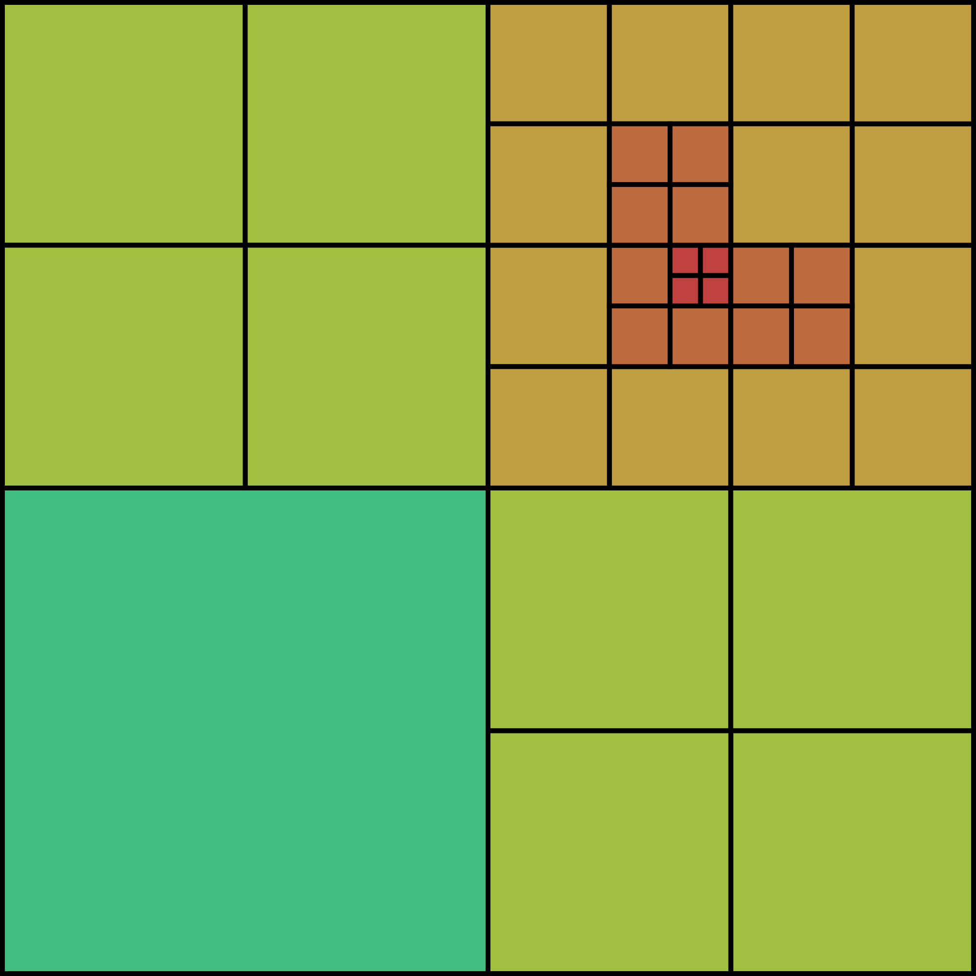
Figure 1: Schematic example of a recursively refined grid structure, of the type bamps employs obeying a $1:2$ condition. This example has $5$ levels of refinement.

III The Physical model

In this section we define the type of initial data we decided to investigate. We then describe the process that allows us to estimate the threshold amplitude within each of the evolved families. Finally we include a description of the post-processing tools that have enabled this estimation.

III.1 Brill waves as initial data

Brill wave initial data are a gravitational-wave solution to vacuum Einstein constraint equations. Following the procedure of Brill [15] it is possible to construct axisymmetric non-linear initial data, where the spatial metric takes the form,

$$dl^{2}=\gamma_{ij}dx^{i}dx^{j}=\Psi^{4}\left[e^{2q}\left(d\rho^{2}+dz^{2}\right)+\rho^{2}d\phi^{2}\right]\,,$$ (5)

and, as the data are taken to be at a moment of time symmetry, the extrinsic curvature vanishes identically. For the seed function we always choose a general Gaussian

$$q(\rho,z)=A\rho^{2}e^{-[(\rho-\rho_{0})^{2}/\sigma_{\rho}^{2}+(z-z_{0})^{2}/\sigma_{z}^{2}]}\,,$$ (6)

whose parameters differ depending on the studied family. In the present work we will focus on six different families always with $z_{0}=0$, $\sigma_{\rho}=\sigma_{z}=1$ covering centered ($\rho_{0}=0$) and off-centered ($\rho_{0}=4$ and $\rho_{0}=5$) Gaussians both prolate ($A>0$) and oblate ($A<0$).

Of these six families, the first ($A>0$, $\rho_{0}=0$) is best studied in the literature, see for example [42, 25, 26, 30, 32]. In [32] the centered oblate family was also treated, and so these two families serve as a point of reference. Khirnov and Ledvinka conclude that these centered families are more difficult to treat numerically than their off-set (constraint solved) Teukolsky wave initial data, which motivates our use of off-center Brill wave data. (See [28] for constrained evolution of alternative Brill wave initial data, which we would also like to compare with in the future).

III.2 Parameter search

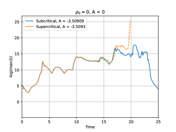
Figure 2: An illustrative figure to show the different behavior for two close sets of initial data. The chosen family is a centered oblate Brill wave $\rho_{0}=0$ with $A<0$. One can see that in the case of the orange dashed line, corresponding to a supercritical amplitude $A=-3.50930$, the maximum of the Kretschmann scalar diverges. On the other hand, in the case of the subcritical amplitude $A=-3.50909$ the Kretschmann’s maximum decreases as the wave disperses.

In order to study phenomena near the threshold of collapse, the first step is to identify that threshold as precisely as we can. With one-parameter families, this is equivalent to identifying the value of the parameter at the threshold. In our case, the parameter varying within a family is the amplitude, $A$, in equation (6). Varying $A$ allows us to classify initial data depending on the outcome of its evolution. Initial data whose evolution yields a dispersal of the fields is classified as subcritical, and data that leads to black hole formation as supercritical,

$$A_{\text{ subcritical}}<A_{\star}<A_{\text{ supercritical}}$$ (7)

(and similarly for families with $A<0$).

In Fig. 2 one can see how the evolution of the logarithm of the maximum of the Kretschmann scalar compares between a subcritical and a supercritical run. This plot illustrates how similar the evolutions of data from the same family can be, up to final times where the one parameter that differentiates them determines dispersal or collapse.

Working with bamps and our AH locator enables the classification as follows:

• At least down to a neighborhood of the threshold, bamps is able to evolve subcritical data until they disperse. We can hence confidently classify the data as subcritical just by looking at all fields dispersing at the end of each evolution. The blue line in Fig. 2 shows the field dispersal of a subcritical run.

• Likewise in Fig. 2 one can see how the orange dashed line, corresponding to a supercritical run, blows up and stops before time $20$. In the present evolutions we are not excising the trapped region, and so in the case of black hole formation, bamps can only evolve for a short time after trapped surface formation. We therefore look for AHs (see section III.3) in the evolved data as a post-processing step. Only when we reliably find horizons do we classify the data as supercritical.

By categorizing the data in this way, we can estimate that the threshold amplitude lies in the regime between the highest subcritical amplitude and the lowest supercritical one. The process of classifying the evolved initial data proceeds in stages, each increasing the precision of our estimation of the threshold, thereby tuning closer to $A_{\star}$.

We employed a modified bisection method to reduce the size of the interval that contains $A_{\star}$. We started the bisection with a guess of trivially weak and strong data. After confirming the limits of the threshold regime, we evolved data within it to further tune those bounds at each stage. We increased the precision of these bounds as far as our methods allowed. Assuming $A_{\star}\in[A_{0},A_{1}]$, the basic bisection method would proceed by choosing $A=(A_{0}+A_{1})/2$, performing an evolution to determine whether the data for $A$ is sub- or supercritical, and adjusting the boundaries of the search interval accordingly. In practice, we divided the threshold regime not into $2$, but typically into $10$ subintervals. Such a bracketed-search strategy can accelerate the search when performing simulations for each $A$ in parallel. (Compare e.g. branch prediction methods in CPU execution pipelines, where different if-clauses are evaluated in parallel, but only the relevant result is used in the end.) When successful, this method adds one decimal place per stage to our limiting amplitudes. This approach furthermore has the advantage that the data necessary for scaling-plots is already prepared directly at the end of bisection without having to go back and resample.

III.3 Apparent Horizon Locator

To conclusively classify a set of initial data as supercritical, the AH finder ahloc3d [43], which is specifically designed for use with bamps AMR data is used. ahloc3d replaces the AH finder employed in [34, 30], which had no functionality with AMR data nor parallelization. During the development of ahloc3d thorough consistency checks were made with the results of the older code.

ahloc3d uses a Strahlkörper representation to describe test surfaces as

$$r =h(\theta,\phi)$$ (8)

relative to a single center point, and evaluates the expansion

$$\Theta =D_{i}s^{i}+\tensor{K}{{}_{i}{}_{j}}s^{i}s^{j}-K\,,$$ (9)

where $s_{i}$ is the outward pointing normal vector on the test surface and $K$ is the extrinsic curvature of the spacetime slice under consideration, according to the algorithm described in [44]. Using two separate search methods, it first obtains a rough estimate using a flow method using the expansion flow [45] to shrink a large test surface until an approximate AH is found, i.e. $\Theta$ satisfies a smallness condition. It then refines this estimate using a Newton-Raphson iteration to locate the AH ($\Theta=0$) with high accuracy. The search algorithm is fully parallelized using MPI. Its main limitation is the Strahlkörper representation of the test surfaces, which makes it unable to find AHs that are not radially convex. As we will discuss below, this has prevented the further fine-tuning of several families of initial data, as the AHs we found approached such non-convex shapes.

IV Numerical Results

In this section we discuss the outcome of the bisection search described in section III for each of our six families.

IV.1 Dynamics and threshold amplitudes

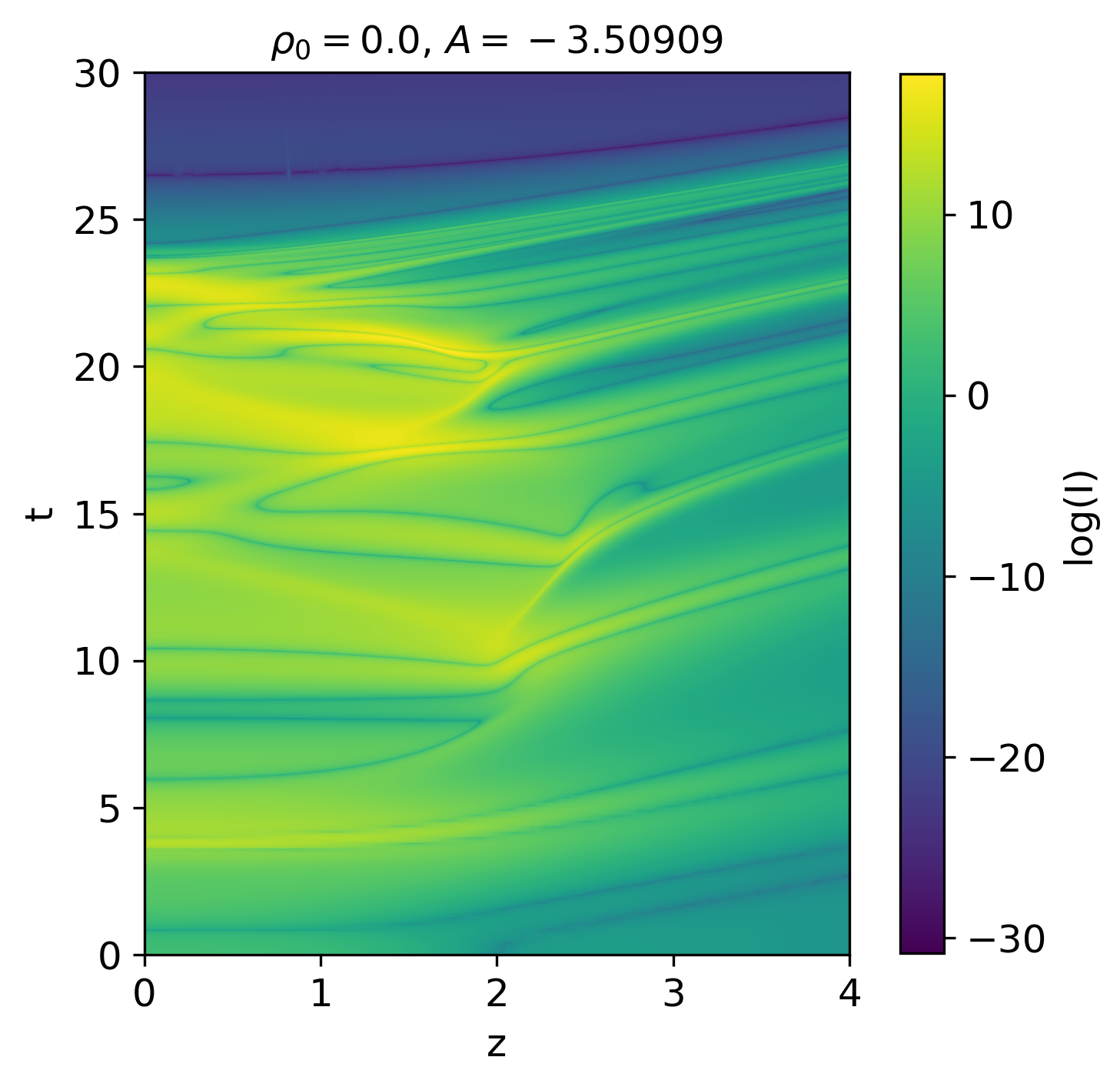
Figure 3: In this figure a color map of the logarithm of the Kretschmann scalar along the symmetry axis and through time is shown for the oblate centered family $A<0$, $\rho_{0}=0$, for the subcritical amplitude $A=-3.50909$.

Basic evolution within each of the families is similar and follows the behavior observed in [30] for the centered $A>0$ family. Very weak data disperse rapidly, but as the strength of the data increases the dynamics become more interesting. Considering the Kretschmann scalar, the simplest non-vanishing curvature scalar in our setup, we see wave-like propagation combined with larger spikes when waves land on the symmetry axis and oscillate there. In comparison with the centered data, the off-center families tend to form these spikes further from the origin, probably because the curvature propagates further in the $\pm z$-directions before hitting the symmetry axis. This difference would have made evolution of the off-center data prohibitively expensive without AMR. To illustrate the dynamics qualitatively, in Fig. 3 we show a 2D plot of the logarithm of the Kretschmann scalar with respect to the symmetry axis and coordinate time for a set of initial data close to criticality ($A=-3.50909$) for the oblate ($A<0$) centered ($\rho_{0}=0$) family. The region shown is relatively small in $z$, but big enough to see that several peaks of the curvature scalar occur away from the origin but along the symmetry axis before they disperse. The results for all of the other families are similar, with more and more off-centered peaks in the Kretschmann scalar appearing as the threshold of black hole formation is approached.

There is a clear distinction between small initial data that lead to dispersion and strong data that ends in the formation of a black hole. The approach we use to classify the data (see subsection III.2) is conservative but, given the challenge these spacetimes pose and the unfortunate occasional disagreement between different numerics, we feel it important to tread lightly, compare carefully with the literature, and indeed to avoid using another proxy for collapse. The results of our bisection search are summarized in Table 1, where we state the highest subcritical and lowest supercritical amplitudes that we were able to classify before ahloc3d failed to find apparent horizons in near threshold simulations. These bounds are compatible with the previous works [30] and [32] for the centered families.

	$\rho_{0}$	$A_{\text{sub}}$	$A_{\text{sup}}$
Prolate ($A>0$)	0	4.69667	4.69680
	4	0.09795	0.09870
	5	0.0641	0.0645
Oblate ($A<0$)	0	-3.50909	-3.50930
	4	-0.07546	-0.07570
	5	-0.04878	-0.04900

Table 1: Results for the limits of the bisection search. The highest subcritical ($A_{\text{sub}}$) and lowest supercritical ($A_{\text{sup}}$) amplitudes for each family are displayed, defining the bounds of the threshold amplitudes.

IV.2 Apparent horizons

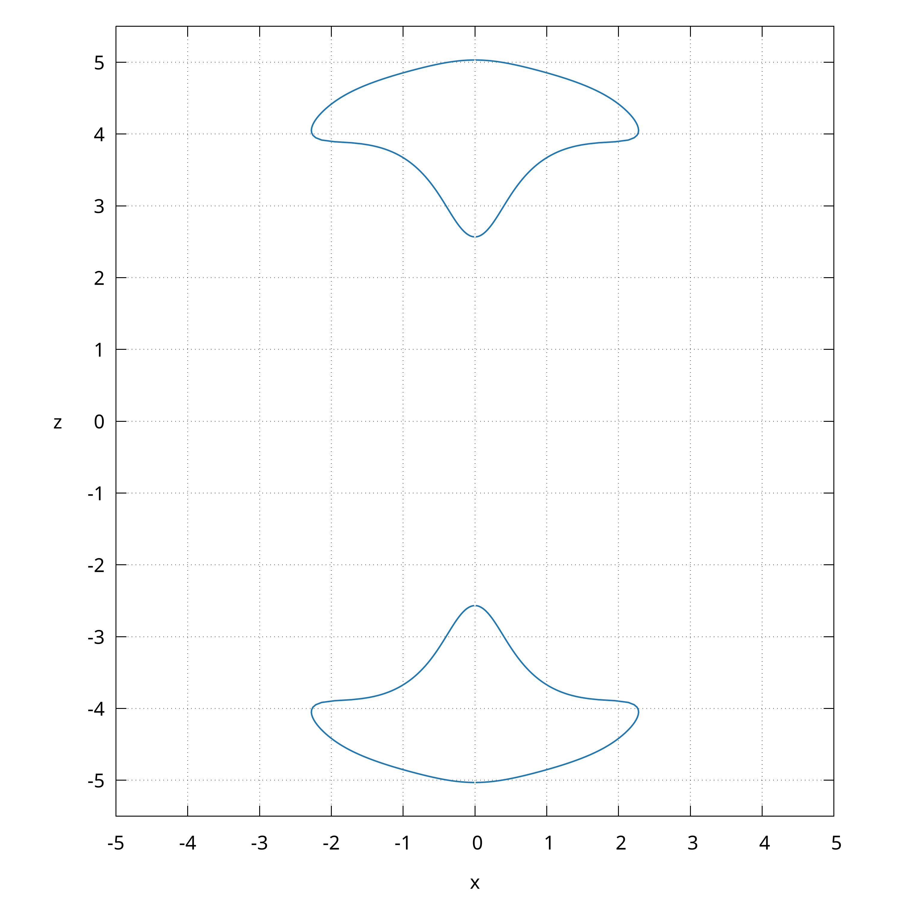
Figure 4: A pair of apparent horizons found by ahloc3d. The horizontal axis represents the x direction and the vertical axis represents the symmetry axis, z. This is for the specific oblate off-centered family $A<0$, $\rho_{0}=4$ with amplitude $A=-0.07570$ at time $t\simeq 25.8$. Comparing, for example, with Fig. $4$ of [30] we see that the apparent horizons are off-set by a greater coordinate distance.

Within a given (supercritical) member of a family, we reliably find AHs after the first has appeared during evolution. In agreement with [30, 32] for the centered prolate family, close to the threshold we find that the AH for the off-centered oblate families bifurcates (observe that this a statement in parameter space, not within an individual spacetime). The AH forms approximately around one of the large peaks in the Kretschmann scalar, along the symmetry axis (forming a binary black hole spacetime if the event horizon shows two components, but we do not investigate event horizons in this work). In Fig. 4 we show this behavior for the oblate ($A<0$), off-centered family $\rho_{0}=4$ with amplitude $A=-0.07570$.

Because of the reflection symmetry of the initial data, the two horizons that appear are perfect copies, symmetric about the equator. We do not have, however, explicit evidence from ahloc3d that the remaining two families (off-center $\rho_{0}=4,5$, prolate $A>0$) also have bifurcated, two-component AHs. To find these, this post-processing software needs to be run close enough to the time of formation of the AH, as shortly after trapped surface formation the underlying numerical evolution will fail. This makes it difficult to hit the right time to search. Despite the lack of explicit evidence, we have strong indications that this is a common feature for all six of the families we studied. Close to the threshold the global peak of the maximum of the Kretschmann scalar always occurs, both for subcritical and supercritical cases, away from the origin and along the symmetry axis. Furthermore, when facing the difficulties with ahloc3d we found some abnormal shapes that are not trustworthy as AH but that seem to indicate that the formation of disjoint AHs is about to occur, or that the has already happened, and that the algorithm of the software needs improvement. Presumably, if we chose initial data without reflection symmetry, and tuned well enough to the threshold, an AH would form only on one side of the equator. Both of the latter two points need further work.

IV.3 Scaling

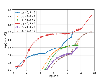
Figure 5: The scaling of the Kretschmann scalar for all the studied families is shown. In the horizontal axis we represent the logarithmic distance to the critical point and in the vertical axis the logarithm of the maximum of the Kretschmann as $I^{(1/4)}$. The red curve compares with Fig. $4$ of [30] and the blue with the green in Fig. $1$ of [32].

According to [3], if critical phenomena are present in the collapse of gravitational waves, any curvature scalar invariant should show universal power-law scaling in the subcritical regime. As we are working in vacuum the Ricci scalar vanishes, so we investigate the scaling behavior of the Kretschmann scalar. In Fig. 5 we plot the logarithm of the maximum of the Kretschmann scalar in the form $I^{1/4}$ against the logarithmic distance to the critical amplitude. (The exponent $\frac{1}{4}$ is chosen to obtain units of one over length.) First, it is clear that the maximum value that the Kretschmann scalar attains depends on the amplitude of the initial data for each family. Second, for each individual family this result is compatible with the power-law behavior in equation (2), and furthermore agrees very well with [30, 32] for the two centered families. There is, however, no evidence of a universal exponent. A priori, this result is compatible with each family having a different exponent, but, extending these lines further to the right (which is very computationally expensive and challenging) would be necessary to make a conclusive statement about universality. If the exponents were truly different, we could wonder whether there exists a finite number of such exponents, leading to a new paradigm of universality, or else, if there are simply as many exponents as families of initial data. Evidently more investigation is needed. Referring to DSS, only one family (the blue curve in Fig. 5) shows enough periods for us to claim that it behaves as approximately-DSS and more periods are needed in the other families. This is also the reason why we postpone treating the errors and interpret this result as qualitative for now.

IV.4 Echoes and universality

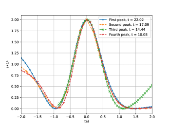
Figure 6: Shown are four echoes for the family of initial data $A<0$, $\rho_{0}=0$ with $A=-3.50909$. Each echo corresponds to a peak of the maximum of the Kretschmann scalar at different times against the proper time. Both axes are rescaled for each curve by the same constant $\lambda$ which is chosen such that the maximum will correspond to $2$ in the plot. The largest ratio of $\lambda$’s across such curves is $\sim 3$.

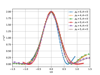
Figure 7: In this figure we show the largest peak of the Kretschmann scalar, for the highest subcritical amplitude of Table 1, for each of the six studied families, against the proper time along the integral curve of $n^{a}$. As in Fig. 6, both the proper time and Kretschmann scalar are rescaled by a constant $\lambda$ chosen such that the maximum of the Kretschmann scalar occurs at 2 in the plot. For these curves the largest ratio of $\lambda$’s is around $10$, corresponding to a ratio $10^{4}$ in the peak of the Kretschmann itself. The data for the prolate ($A>0$) off-centered families and for the oblate ($A<0$) centered family have been flipped along the horizontal axis for a better match.

In the case of a massless scalar field collapse in spherical symmetry [1], the critical solution shows DSS behavior, however, in the axisymmetric collapse of gravitational waves in vacuum the picture is more complicated. As discussed above, we observe that for a near threshold evolution $A\lesssim A_{\star}$ (flipped for $A<0$ families), several large local peaks in the Kretschmann scalar appear along the symmetry axis before the data eventually disperse. In Fig. 6 we plot these peaks against proper time along timelike curves (the integral curves of the unit normal vector $n^{a}$) that pass through the maxima (one curve per peak), and compare their shape by rescaling them with a constant $\lambda$ so that we plot dimensionless quantities on both axes. In the figure, we take the oblate ($A<0$) centered family $\rho_{0}=0$. We allow ourselves the freedom to flip the axis for individual curves to take care of features propagating up or down the $z$-axis. The agreement of the four curves is striking, especially given that the values of $\lambda$ for each of the curves vary by a factor of $\sim 3$, corresponding to a little less than two orders of magnitude in the Kretschmann scalar itself. Four echoes were found for four different times, in qualitative agreement with [32] where they show in Fig. 3 a similar plot for a Teukolsky wave. It is important to remark that this feature is exclusive to near threshold evolutions. In contrast, for small initial data only one peak of the Kretschmann scalar occurs, and no such repeated features appear. Analogous results were found in all of the other families, however, the echoing is not as clean as for the displayed family. Given that $A-A_{\star}$ has no absolute meaning, one might argue that for the other families our data are not close enough to the threshold solution to show such good results. On the symmetry axis, the scalar quantity studied by Ledvinka and Khirnov in [32] is directly related to the Kretschmann scalar. One might expect their profiles to agree with ours, but, the normal vector associated with the foliation of [32] does not coincide with ours, and thus the integral curves along which we plot do not either. We thus postpone a detailed comparison. We have not identified clearly whether these repeated features correspond to true DSS behavior. In our coordinates they appear without regular time intervals, and our curvature scaling plots indicate neither universal power-laws nor uniformly periodic wiggles, so we have no reason to expect true DSS. That said, this is clear evidence of phenomenology familiar from the spherical setting carrying over.

In order to compare the spacetime behavior among families, in Fig. 7 we plot the profile of the Kretschmann scalar against the proper time along a timelike curve that passes through the maxima, for near critical data as done in Fig. 6, but for the largest peak within our best-tuned data within each different family. Each of these lines corresponds to the most right placed point of Fig. 5 for each family, being as close to the threshold solution as possible. Again the shapes around the peaks agree, showing a common feature that appears when evolving initial data with amplitude $A\simeq A_{\star}$ independently of the chosen family of initial data, and again, in concordance with [32].

V Summary and discussion

Earlier work [30] on gravitational wave collapse with bamps was severely hampered by the rapidly increasing computational cost near the threshold. With an allocation of around $10$ million core hours, in that study we were able to tune just a single family to the threshold of collapse. For that reason bamps has undergone a major overhaul, and now fully supports adaptive mesh-refinement, the details of which will appear in a stand-alone report. Presently, with a similar allocation we were able to tune six families to within a comparable distance to the threshold of collapse. What is more, it is expected that as we now push even closer to the threshold and progressively finer spacetime features appear, this improvement in efficiency will become ever more pronounced.

The obvious question is then, with this additional efficiency why have we not already pushed one (or more) of our families closer to the threshold? The answer is that we still encounter difficulties in the bisection, and in particular in classifying spacetimes close to the threshold. There are two main reasons for this; first, we cannot preclude the formation of coordinate singularities, which no amount of AMR could cure, and which would prevent classification if they appear before trapped surface formation. The choice of the gauge parameter $\eta_{S}$ as defined in (4) for instance appears to be highly important. Related to this is the appearance of constraint violation, which does get worse in the strong-field regime and especially in the presence of fine features (but which we believe is not the leading problem in our present data). Unsurprisingly we found that our evolutions were more numerically challenging close to the threshold. Constraint violation does get worse near the threshold. Usually the constraint violation stays in a range of about $10^{-8}$ to $10^{-6}$ for small initial data. However, when the Kretschmann scalar grows this violation might reach up to $10^{-3}$, but still remains several orders of magnitude smaller than the relevant evolved quantities. The second issue we encountered was that, particularly for the off-centered families, the shapes of the apparent horizons change drastically the closer we get to the threshold. We suspect that there may be AHs which cannot be captured by ahloc3d due to the Strahlkörper representation described in section III.3. Fortunately, strategies are available to avoid both of these issues in the future.

Despite these shortcomings, our setup allows careful examination of the threshold of black hole formation of axisymmetric gravitational waves, which is, by default, beyond spherical symmetry in $3+1$ spacetime dimensions. Close to the threshold, we find explicitly that three of our six families form two disjoint apparent horizons. In the remaining three families we expect the same because the spikes in the Kretschmann scalar form away from the origin. These spikes are further separated for off-center data than for centered data. In hindsight, this was perhaps foreseeable because, since our seed functions were off-set in the cylindrical polar direction $\rho$, the waves have time to propagate in the $z$-direction before they hit the symmetry axis. It would be interesting to evolve initial data families off-set in both $\rho$ and $z$ to examine how generic the appearance of pairs of AHs is within families of reflection symmetric data. With the (constraint solved) Teukolsky waves of [32] and the present work, this does however appear a fairly robust feature.

Our results for the scaling of the Kretschmann scalar shown in Fig. 5 agree perfectly with [30, 32], making us confident that our code is reliable as we were able to reproduce results for the centered Brill waves. Our main objective was to help establish the extent to which the standard picture of critical collapse extends beyond spherical symmetry. As discussed in the introduction, a number of studies suggest that this story is a subtle one, and the present work further reinforces this perspective. We examined four families of off-center initial data for the first time. Considering the scaling plot for each family individually, it is tempting to argue that the data take the form of a power-law plus a possibly periodic wiggle. But at least to the level of tuning we have presented here, there appears to be neither a universal power nor period in the wiggle. It is possible that we simply need greater numerical accuracy, but given the solid agreement with the independent implementation in [32] that does seem unlikely. The evidence at hand thus suggests that the exponents of the respective power-laws and periods of the wiggles, if the latter can even be defined, are family dependent. Presumably, this corresponds to the manifestation of different threshold solutions, and so departs from the standard picture in spherical symmetry. Assuming this is the case, a natural question is whether threshold solutions can be well described by a finite, countable, or uncountable number of parameters. Much more work is needed to shed light on this question.

Most interestingly, our evidence strongly suggests that aspects of behavior familiar from the spherical setting do carry over. Looking at Fig. 7, it is clear that, close enough to the threshold solution, all six of our families present strikingly similar behavior for the Kretschmann scalar, with a peak of practically the same shape appearing at different scales. This is a clear indication that some kind of universality still remains. This is furthermore in good agreement with the findings by [32] for alternative families of initial data. Likewise we also find, within individual families, that repeated echoes appear in the curvature scalar.

There are a number of obvious ways in which to extend our work. First, improvements to ahloc3d are needed so that the apparent horizons that do not follow the Strahlkörper parametrization can be found (see [46], where the same problem was faced, for a possible solution). It could be possible to analyze even the sets of data that were currently produced within this work to push these same bisection searches further. Next, is the treatment of alternative families, including radially off-set Brill waves and (constraint solved) Teukolsky waves. We also expect that finer control of constraint violation and coordinates would be of benefit. For the latter we have already implemented the DF-GHG formulation [47, 48, 49], but the complete generalization of the outer boundary conditions to that setting is ongoing. A further question, already mentioned in passing in [30], is whether or not the curvature spikes we observe have anything to do with BKL behavior. As such, following [50], it would be interesting to calculate the expected behavior of the Kretschmann scalar for comparison. Ultimately, as bamps undergoes further development, we aim to relax our symmetry assumptions, to make full 3d evolutions at the threshold of vacuum collapse possible. Progress on all of these fronts will be reported elsewhere.