Data Size-Aware Downlink Massive MIMO:
A Session-Based Approach

Abstract

This letter considers the development of transmission strategies for the downlink of massive multiple-input multiple-output networks, with the objective of minimizing the completion time of the transmission. Specifically, we introduce a session-based scheme that splits time into sessions and allocates different rates in different sessions for the different users. In each session, one user is selected to complete its transmission and will not join subsequent sessions, which results in successively lower levels of interference when moving from one session to the next. An algorithm is developed to assign users and allocate transmit power that minimizes the completion time. Numerical results show that our proposed session-based scheme significantly outperforms conventional non-session-based schemes.

I Introduction

We are witnessing an explosion of streaming and learning applications, such as video streaming, live conferencing, and federated learning [1, 2, 3]. Many of these applications require computations by mobile users (UEs) [4], and the UEs have fixed amounts of data to receive. To support these applications, it is critical to design transmission schemes that achieve low latency. It is of particular importance to design communication protocols that minimize the completion time, defined as the time it takes for a UE to receive all data destined for it.

To support the aforementioned applications, massive multiple-input multiple-output (MIMO) can be used due to its ability to offer high data rates to all UEs simultaneously [5]. To reduce the completion time, conventionally, the achievable rates of all the UEs are maximized via power allocation, and these rates are kept constant during the whole transmission. Another approach is to use different rates during the transmission period [6]. When some UEs have already completed their transmissions, other UEs will benefit by having less multi-user interference and higher rates, which results in shorter completion times. In this context, [6] studies the completion time for two-user systems from an information-theoretic perspective. However, general schemes for multi-user systems that use different rates within the transmission period have not been explored in the literature.

Contributions: Motivated by [6], we introduce a session-based scheme to reduce the completion times of UEs for the downlink of massive MIMO networks. In this scheme, UE data is transmitted with different rates in different sessions. Specifically, in each session, UEs are assigned so that one UE finishes its transmission and does not participate in subsequent sessions. UEs with uncompleted transmissions are allocated more power to obtain higher achievable rates, and complete their transmissions faster. Herein, zero-forcing (ZF) processing is used for data transmission. An algorithm is developed for assigning UEs and allocating transmit power, with the objective of minimizing the completion times of the UEs. Numerical results show that the proposed session-based scheme significantly reduces the completion times compared to conventional transmission that relies on power control only.

A specific version of this session-based scheme was also used in [7], although for a different objective and for a particular application. Herein, we substantially extend [7] to the general problem of minimizing downlink completion times. If the amounts of UE data in each session are given, then the optimization problem reduces to power and rate control for conventional transmission (with different rate constraints for different users). However, optimizing the amounts of data per session and the thresholds for the rate constraints over multiple sessions is a new and challenging problem.

II System Model

We consider the downlink transmission in a massive MIMO network, where an $M$-antenna base station (BS) serves $K\leq M$ single-antenna UEs simultaneously in the same frequency band. Let $S_{k}$ be the size of the data intended for UE $k$. We focus on applications where $S_{k}$ is fixed, such as mobile edge computing and federated learning to name but a few [8, 3]. We assume that the transmission time is within one large-scale coherence time, and the transmission is spans multiple small-scale coherence blocks. A small-scale coherence block is the time-frequency interval over which the channel is substantially static, and is divided into two phases: channel estimation and downlink payload data transmission.

Resource allocation, such as transmit power control, is typically performed to guarantee given quality-of-service targets. We consider two conventional schemes: (i) Conventional non-data size-aware scheme: This scheme allocates power such that all users achieve the same rate [5]; and (ii) Conventional data size-aware scheme: This scheme allocates power such that each UE receives a rate proportional to the size of its data. This is the traditional scheme used in wireless networks supporting mobile edge computing or federated learning (see, e.g., [8, 3] and references therein).

In both conventional schemes, the data rates are kept fixed for the whole transmission. However, since $K$ UEs have different required data sizes, some UEs could complete their transmissions before other UEs. Therefore, optimally, the data rates vary temporally depending on how many active UEs remain in the system. The main question is how to allocate power and update the UEs’ rates to reduce the completion times. Motivated by this, we next propose the novel session based-scheme.

III Proposed Session-Based Scheme

Our proposed scheme uses different rates in different time periods for data transmissions. The transmission period during which the rates are kept fixed is called a “session”. More precisely, session $i$ is defined as follows: (i) in session $i$, there are $K-i+1$ active UEs; and (ii) at the beginning of session $i$, the BS updates the rates for these active UEs. These rates will be kept fixed until the end of this session, where one UE completes receiving data from the BS. Thus, the BS transmits data to all $K$ UEs during $K$ sessions. Fig. 1 illustrates the proposed session-based transmission as well as conventional transmission for a system with three UEs. Denote by $a_{i}$ the indicator that is defined as

$$a_{k,i}\triangleq\begin{cases}1,&\text{if UE $k$ is receiving data in session $i$,}\\ 0,&\mbox{otherwise}.\end{cases}$$ (1)

Denote by $\operatorname{\mathcal{K}}_{i}\triangleq\{k|a_{k,i}=1\}$ the set of $K_{i}=\sum_{k\in\operatorname{\mathcal{K}}}a_{k,i}$ UEs assigned in session $i\in\operatorname{\mathcal{K}}$, where $\operatorname{\mathcal{K}}=\{1,2,\ldots,K\}$. Then, we have

$$a_{k,1}=1,\sum_{k\in\operatorname{\mathcal{K}}}a_{k,i}=K-i+1,a_{k,i}\leq a_{k,i-1},\forall i,$$ (2)

to ensure that all the UEs will be served in session $1$. In each subsequent session, one UE completes its transmission and will not join the next sessions. As such, more power is allocated to the UEs that have not yet completed their transmissions. Note that, the conventional (non-session-based) schemes are special cases of the proposed scheme when all UEs are served in session $1$ with $a_{k,1}=1,\forall k$.

Uplink channel estimation: In each small-scale coherence block of length $\tau_{c}$, each UE sends its pilot of length $\tau_{p}$ to the BS. We assume that all pilots are mutually orthogonal, which requires $\tau_{p}\geq K$. Denote by $\operatorname{\boldsymbol{g}}_{k}\!=\!(\beta_{k})^{1/2}\tilde{\operatorname{\boldsymbol{g}}}_{k}$ the channel vector from UE $k$ to the BS, where $\beta_{k}$ and $\tilde{\operatorname{\boldsymbol{g}}}_{k}$ are the large-scale fading coefficient and small-scale fading vector, respectively. With minimum mean-square error (MMSE) estimation, the channel estimate $\hat{\operatorname{\boldsymbol{g}}}_{k}$ of $\operatorname{\boldsymbol{g}}_{k}$ is distributed according to $\operatorname{\mathcal{CN}}(\boldsymbol{0},\sigma_{k}^{2}\boldsymbol{I}_{M})$, where $\sigma_{k}^{2}=\frac{\tau_{p}\rho_{p}\beta_{k}^{2}}{\tau_{p}\rho_{p}\beta_{k}+1}$, and $\rho_{p}$ is the normalized transmit power of each pilot symbol [5, (3.8)]. Let $\hat{\operatorname{\boldsymbol{G}}}_{i}\triangleq[\hat{\operatorname{\boldsymbol{g}}}_{1},\dots,\hat{\operatorname{\boldsymbol{g}}}_{K-i+1}],\forall k\in\operatorname{\mathcal{K}}_{i}$, be the matrix stacking the estimated channels of all participated UEs in session $i$.

Downlink payload data transmission: In session $i$, the BS uses ZF to transmit data to $K-i+1$ UEs. With ZF, the signal transmitted by the BS is given by $\operatorname{\boldsymbol{x}}_{i}\!\!=\!\!\sqrt{\rho}\sum_{k\in\operatorname{\mathcal{K}}_{i}}\operatorname{\boldsymbol{u}}_{k,i}s_{k,i}$, where $\rho$ is the normalized transmit power at the BS; $s_{k,i}$, with $\operatorname{\mathbb{E}}\{|s_{k,i}|^{2}\}=1$, is the symbol intended for UE $k$; and $\operatorname{\boldsymbol{u}}_{k,i}\!=\!\sqrt{\eta_{k,i}{\sigma}_{k}^{2}(M\!-\!K_{i})}\hat{\operatorname{\boldsymbol{G}}}_{i}(\hat{\operatorname{\boldsymbol{G}}}_{i}^{H}\hat{\operatorname{\boldsymbol{G}}}_{i})^{-1}\operatorname{\boldsymbol{e}}_{k,K_{i}}$ is the ZF precoding vector. Here, $\operatorname{\mathbb{E}}\{x\}$ denotes the expected value of a random variable $x$, and $\boldsymbol{X}^{H}$ represents the conjugate transpose of a matrix $\boldsymbol{X}$. In the precoding vector, $\eta_{k,i}$ is a power control coefficient, and $\operatorname{\boldsymbol{e}}_{k,K_{i}}$ is the $k$-th column of $\boldsymbol{I}_{K_{i}}$. The transmitted power at the BS is constrained by $\operatorname{\mathbb{E}}\{|\operatorname{\boldsymbol{x}}_{i}|^{2}\}\leq\rho$ which is equivalent to

$$\sum_{k\in\operatorname{\mathcal{K}}_{i}}\eta_{k,i}\leq 1,\forall i\in\operatorname{\mathcal{K}}.$$ (3)

We enforce

$$(\eta_{k,i}=0,\text{if $a_{k,i}=0$}),\forall k,i$$ (4)

to ensure that the BS will not allocate any power to UEs that are not served in session $i$. The achievable rate at UE $k$ in session $i$ is given by [5, Eq. (3.56)]: $R_{k,i}(\operatorname{\boldsymbol{\eta}}_{i})=\frac{\tau_{c}-\tau_{p}}{\tau_{c}}B\log_{2}\big{(}1+\text{SINR}_{k,i}(\operatorname{\boldsymbol{\eta}}_{i})\big{)}$, where $B$ is the bandwidth, $\text{SINR}_{k,i}(\operatorname{\boldsymbol{\eta}}_{i})=\frac{(M-K_{i})\rho\hat{\sigma}_{k}^{2}\eta_{k,i}}{\rho(\beta_{k}-{\sigma}_{k}^{2})\sum_{\ell\in\operatorname{\mathcal{K}}_{i}}\eta_{\ell,i}+1}\overset{\eqref{eta-a-relation}}{=}\frac{(M-K_{i})\rho{\sigma}_{k}^{2}\eta_{k,i}}{\rho(\beta_{k}-\hat{\sigma}_{k}^{2})\sum_{\ell\in\operatorname{\mathcal{K}}}\eta_{\ell,i}+1}$ is the effective downlink signal-to-interference-plus-noise ratio (SINR), and $\operatorname{\boldsymbol{\eta}}_{i}\triangleq\{\eta_{k,i}\}_{k\in\operatorname{\mathcal{K}}}$.

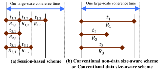
Figure 1: One transmission period with three UEs.

Completion time: Let $S_{k,i}$ be the size of the data sent to UE $k$ in session $i$. Then, we have

$$\sum_{i\in\operatorname{\mathcal{K}}}S_{k,i}=S_{k},\forall k.$$ (5)

Let $t_{i}$ be the time duration of session $i$. Then, the transmission time $t_{k,i}$ of UE $k\in\operatorname{\mathcal{K}}$ in session $i$ is given by

$$t_{k,i}\!=\!a_{k,i}t_{i},\forall k,i.$$ (6)

Thus,

$$S_{k,i}\!=\!R_{k,i}(\operatorname{\boldsymbol{\eta}}_{i})t_{k,i}\!\overset{\eqref{tdki}}{=}\!R_{k,i}(\operatorname{\boldsymbol{\eta}}_{i})a_{k,i}t_{i}\!\overset{\eqref{eta-a-relation}}{=}\!R_{k,i}(\operatorname{\boldsymbol{\eta}}_{i})t_{i},\forall k,i.$$ (7)

Clearly, (7) also implies that $(S_{d,k,i}=0,\text{if $a_{k,i}=0$}),\forall k,i$. The completion time of UE $k$ is the sum of its transmission times across all sessions, i.e., $\sum_{i\in\operatorname{\mathcal{K}}}a_{k,i}t_{i}$. Let $\widetilde{T}_{c}$ and $T_{c}$ the large-scale and small-scale coherence times, respectively. Since each session spans multiple small-scale coherence blocks but always fits within one large-scale coherence time, we have

$$T_{c}\leq t_{i},\forall i$$ (8)

$$\sum_{i\in\operatorname{\mathcal{K}}}t_{i}\leq\widetilde{T}_{c}.$$ (9)

Remark 1.

In this work, in order to focus on fundamental principles of the proposed scheme, that is, UE assignment and rate allocation, we consider independent Rayleigh channels. The optimization and analysis of a session-based scheme tailored to correlated channels is interesting, but analytically challenging and beyond the scope of the paper. Thus, such designs are left for future work.

IV Completion Time Minimization

We address the minimization of the completion time of our proposed session-based scheme, and specifically minimizing the longest completion time among the UEs. For comparison, we also include the completion time minimization for the conventional schemes.

IV-A Proposed Session-Based Scheme

The problem of minimizing the completion time of UEs by optimizing the UE assignment ($\operatorname{\boldsymbol{a}}$) and transmit power ($\operatorname{\boldsymbol{\eta}}$) in the session-based design is

$$\!\!\!\!\!\underset{\operatorname{\boldsymbol{x}}}{\min}\,\, \max_{k}\sum_{i\in\operatorname{\mathcal{K}}}a_{k,i}t_{i},$$ (10a)

$$\!\!\!\!\!\mathrm{s.t.}\,\, \eqref{a}-\eqref{eta-a-relation},\eqref{samesizedatad},\eqref{sametime:sessisionS1}-\eqref{large-scale:session:relation}$$

$$0\leq\eta_{k,i},\forall k,i,$$ (10b)

where $\operatorname{\boldsymbol{x}}\triangleq\{\operatorname{\boldsymbol{a}},\operatorname{\boldsymbol{\eta}},\operatorname{\boldsymbol{S}},\operatorname{\boldsymbol{t}}\}$, $\operatorname{\boldsymbol{S}}\!\triangleq\{S_{k,i}\}$, $\operatorname{\boldsymbol{a}}\triangleq\{a_{k,i}\}$, $\operatorname{\boldsymbol{t}}\triangleq\{t_{i}\}$ $\forall k,i$.

Finding a globally optimal solution to problem (10) is challenging due to the mixed-integer and nonconvex constraints (1), (4), and (7). Thus, we instead propose an approach that is suitable for practical implementation. First, we replace constraint (4) by

$$\eta_{k,i}\leq a_{k,i},\forall k,i,$$ (11)

and constraint (7) by

$$S_{k,i}\leq R_{k,i}(\operatorname{\boldsymbol{\eta}}_{i})a_{k,i}t_{i},\forall k,i$$ (12)

$$S_{k,i}\geq R_{k,i}(\operatorname{\boldsymbol{\eta}}_{i})a_{k,i}t_{i},\forall k,i.$$ (13)

We further replace constraints (12) and (13) by

$$\hat{r}_{k,i}\leq R_{k,i}(\operatorname{\boldsymbol{\eta}}_{i}),\forall k,i$$ (14)

$$\tilde{r}_{k,i}\geq R_{k,i}(\operatorname{\boldsymbol{\eta}}_{i}),\forall k,i$$ (15)

$$\hat{t}_{k,i}\leq a_{k,i}t_{i},\forall k,i$$ (16)

$$\tilde{t}_{k,i}\geq a_{k,i}t_{i},\forall k,i$$ (17)

$$S_{k,i}\leq\hat{r}_{k,i}\hat{t}_{k,i},\forall k,i$$ (18)

$$S_{k,i}\geq\tilde{r}_{k,i}\tilde{t}_{k,i},\forall k,i,$$ (19)

where $\hat{\operatorname{\boldsymbol{r}}}\triangleq\{\hat{r}_{k,i}\},\tilde{\operatorname{\boldsymbol{r}}}\triangleq\{\tilde{r}_{k,i}\},\hat{\operatorname{\boldsymbol{t}}}\triangleq\{\hat{t}_{k,i}\},\tilde{\operatorname{\boldsymbol{t}}}\triangleq\{\tilde{t}_{k,i}\}$ are additional variables. We observe from (14)–(18) that $S_{k,i}\leq\tilde{r}_{k,i}\tilde{t}_{k,i},\forall k,i$. Thus, (19) is equivalent to

$$V_{1}(\tilde{\operatorname{\boldsymbol{r}}},\tilde{\operatorname{\boldsymbol{t}}},\operatorname{\boldsymbol{S}}) \triangleq\sum_{k\in\operatorname{\mathcal{K}}}\sum_{i\in\operatorname{\mathcal{K}}}(\tilde{r}_{k,i}\tilde{t}_{k,i}-S_{k,i})\leq 0.$$ (20)

Now, in order to handle the binary constraint (1), we note that $x\in\{0,1\}\Leftrightarrow x\in[0,1]\,\&\,x-x^{2}\leq 0$ [9]. Thus, (1) can be replaced by the following equivalent constraints:

$$\!\!\!V_{2}(\operatorname{\boldsymbol{a}})\triangleq\sum_{k\in\operatorname{\mathcal{N}}}\sum_{i\in\operatorname{\mathcal{K}}}(a_{k,i}\!-\!a_{k,i}^{2})\leq 0$$ (21)

$$\!\!0\leq a_{k,i}\!\leq 1,\forall k,i.$$ (22)

Then, problem (10) is written into a more tractable form as

$$\underset{\widetilde{\operatorname{\boldsymbol{x}}}}{\min}\,\, q$$ (23a)

$$\mathrm{s.t.}\,\, \eqref{sumaki},\eqref{powerdupperbound},\eqref{samesizedatad},\eqref{small-scale:session:relation},\eqref{large-scale:session:relation},\eqref{powerlowerbound},\eqref{power-a-relation},\eqref{ratedki-lowerbound-1}-\eqref{sametime:sessisionS1-1-a},\eqref{V1}-\eqref{arelax}$$

$$\sum_{i\in\operatorname{\mathcal{K}}}\tilde{t}_{k,i}\leq q,\forall k,i,$$ (23b)

where $\widetilde{\operatorname{\boldsymbol{x}}}\!\triangleq\!\{\operatorname{\boldsymbol{x}},\hat{\operatorname{\boldsymbol{r}}},\tilde{\operatorname{\boldsymbol{r}}},\hat{\operatorname{\boldsymbol{t}}},\tilde{\operatorname{\boldsymbol{t}}},q\}$, and $q$ is an additional variable. Let $\operatorname{\mathcal{F}}\!\triangleq\!\{\eqref{sumaki},\eqref{powerdupperbound},\eqref{samesizedatad},\eqref{small-scale:session:relation},\eqref{large-scale:session:relation},\eqref{powerlowerbound},\eqref{power-a-relation},\eqref{ratedki-lowerbound-1}-\eqref{sametime:sessisionS1-1-a},\eqref{V1}-\eqref{arelax},\eqref{q:lb}\}$ be the feasible set of problem (23). We consider the problem

$$\underset{\widetilde{\operatorname{\boldsymbol{x}}}\in\widehat{\operatorname{\mathcal{F}}}}{\min}\,\, \operatorname{\mathcal{L}}(\operatorname{\boldsymbol{a}},\tilde{\operatorname{\boldsymbol{r}}},\tilde{\operatorname{\boldsymbol{t}}},\operatorname{\boldsymbol{S}},\lambda),$$ (24)

where $\operatorname{\mathcal{L}}(\operatorname{\boldsymbol{a}},\tilde{\operatorname{\boldsymbol{r}}},\tilde{\operatorname{\boldsymbol{t}}},\operatorname{\boldsymbol{S}},\lambda)\triangleq q\!+\!\lambda(\gamma_{1}V_{1}(\tilde{\operatorname{\boldsymbol{r}}},\tilde{\operatorname{\boldsymbol{t}}},\operatorname{\boldsymbol{S}})+\gamma_{2}V_{2}(\operatorname{\boldsymbol{a}}))$ is the Lagrangian of (23), $\gamma_{1},\gamma_{2}>0$ are fixed weights, and $\lambda$ is the Lagrangian multiplier corresponding to constraints (20), (21). Here, $\widehat{\operatorname{\mathcal{F}}}\triangleq\operatorname{\mathcal{F}}\setminus\{\eqref{V1},\eqref{V2}\}$.

Proposition 1.

The values $V_{1,\lambda}$ and $V_{2,\lambda}$ of $V_{1}$ and $V_{2}$ at the solution of (24) corresponding to $\lambda$ converge to $0$ as $\lambda\rightarrow+\infty$. Moreover, problem (23) has strong duality, i.e.,

$$\underset{\widetilde{\operatorname{\boldsymbol{x}}}\in\operatorname{\mathcal{F}}}{\min}\,\,q=\underset{\lambda\geq 0}{\sup}\,\,\underset{\widetilde{\operatorname{\boldsymbol{x}}}\in\widehat{\operatorname{\mathcal{F}}}}{\min}\,\,\operatorname{\mathcal{L}}(\operatorname{\boldsymbol{a}},\tilde{\operatorname{\boldsymbol{r}}},\tilde{\operatorname{\boldsymbol{t}}},\operatorname{\boldsymbol{S}},\lambda),$$ (25)

and consequently, (23) is equivalent to (24) at the optimal solution $\lambda^{*}\geq 0$ of the sup-min problem in (25).

Proof.

See Appendix. ∎

Theoretically, it is required to have $V_{1,\lambda}=0$ and $V_{2,\lambda}=0$ in order to obtain the optimal solution to problem (23). By Proposition 1, $V_{1,\lambda}$ and $V_{2,\lambda}$ converge to $0$ as $\lambda\to+\infty$. In practice, it is sufficient to accept $V_{1,\lambda}\leq\varepsilon,V_{2,\lambda}\leq\varepsilon$ for some small $\varepsilon$ with a sufficiently large value of $\lambda$. In our numerical experiments, for $\varepsilon=10^{-3}$, we see that $\lambda=1$ with $\gamma_{1}=0.1,\gamma_{2}=0.01$ is enough to ensure that $V_{1,\lambda}\leq\varepsilon,V_{2,\lambda}\leq\varepsilon$. This way of choosing $\lambda$ has been widely used in the literature, e.g., see [9] and references therein.

Problem (24) is still difficult to solve due to the nonconvex constraints (14)–(18), and nonconvex parts $V_{1}(\operatorname{\boldsymbol{a}}),V_{2}(\tilde{\operatorname{\boldsymbol{r}}},\tilde{\operatorname{\boldsymbol{t}}},\operatorname{\boldsymbol{S}})$ in the cost function $\operatorname{\mathcal{L}}(\operatorname{\boldsymbol{a}},\tilde{\operatorname{\boldsymbol{r}}},\tilde{\operatorname{\boldsymbol{t}}},\operatorname{\boldsymbol{S}},\lambda)$. To deal with (14), we observe that $\log\big{(}1+\frac{x}{y}\big{)}\geq\log\big{(}1+\frac{x^{(n)}}{y^{(n)}}\big{)}+\frac{2x^{(n)}}{(x^{(n)}+y^{(n)})}-\frac{(x^{(n)})^{2}}{(x^{(n)}+y^{(n)})x}-\frac{x^{(n)}y}{(x^{(n)}+y^{(n)})y^{(n)}}$, where $x>0,y>0$ [10, Eq. (76)]. Therefore, the concave lower bound $\widehat{R}_{d,k,i}(\operatorname{\boldsymbol{\eta}}_{i})$ of $R_{d,k,i}(\operatorname{\boldsymbol{\eta}}_{i})$ is given by $\widehat{R}_{d,k,i}\triangleq\frac{\tau_{c}-\tau_{p}}{\tau_{c}\log 2}B\Big{[}\log\big{(}1+\frac{\Upsilon_{i}^{(n)}}{\Phi_{i}^{(n)}}\big{)}+\frac{2\Upsilon_{i}^{(n)}}{(\Upsilon_{i}^{(n)}+\Phi_{i}^{(n)})}-\frac{(\Upsilon_{i}^{(n)})^{2}}{(\Upsilon_{i}^{(n)}+\Phi_{i}^{(n)})\Upsilon_{i}}-\frac{\Upsilon_{i}^{(n)}\Phi}{(\Upsilon_{i}^{(n)}+\Phi_{i}^{(n)})\Phi_{i}^{(n)}}\Big{]}$, where $\Upsilon_{i}(\eta_{k,i})\triangleq(M-K_{i})\rho\hat{\sigma}_{k}^{2}\eta_{k,i}$ and $\Phi_{i}(\operatorname{\boldsymbol{\eta}}_{i})\triangleq\rho(\beta_{k}-\sigma_{k}^{2})\sum_{\ell\in\operatorname{\mathcal{K}}}\eta_{\ell,i}+1$. Then (14) can be approximated by the following convex constraint

$$\hat{r}_{k,i}\leq\widehat{R}_{k,i}(\operatorname{\boldsymbol{\eta}}_{i}),\forall k,i.$$ (26)

To deal with constraints (15), we observe that $\log\big{(}1+\frac{x}{y}\big{)}\leq\log\big{(}x^{(n)}+y^{(n)}\big{)}+\frac{x+y-x^{(n)}-y^{(n)}}{x^{(n)}+y^{(n)}}-\log(y)$, where $x>0,y>0$. Therefore, the convex upper bound $\widetilde{R}_{k,i}(\operatorname{\boldsymbol{\eta}}_{i})$ of $R_{k,i}(\operatorname{\boldsymbol{\eta}}_{i})$ is expressed as $\widetilde{R}_{d,k,i}\triangleq\frac{\tau_{c}-\tau_{u,p}}{\tau_{c}\log 2}B\Big{[}\log\big{(}\Upsilon_{i}^{(n)}+\Phi_{i}^{(n)}\big{)}+\frac{\Upsilon_{i}+\Phi_{i}-\Upsilon_{i}^{(n)}-\Phi_{i}^{(n)}}{\Upsilon_{i}^{(n)}+\Phi_{i}^{(n)}}-\log(\Phi_{i})\Big{]}$. Thus, constraint (15) can be approximated by the following convex constraint

$$\tilde{r}_{k,i}\geq\widetilde{R}_{k,i}(\operatorname{\boldsymbol{\eta}}_{i}),\forall k,i.$$ (27)

Next, we observe that $xy\leq 0.25[(x+y)^{2}-2(x^{(n)}-y^{(n)})(x-y)+(x^{(n)}-y^{(n)})^{2}]$ and $-xy\leq 0.25[(x\!-\!y)^{2}\!-\!2(x^{(n)}\!+\!y^{(n)})(x\!+\!y)+(x^{(n)}+y^{(n)})^{2}],\forall x\geq 0,y\geq 0,z\geq 0$ [3]. Therefore, (16)–(18) can be approximated by the following convex constraints

$$\hat{t}_{d,k,i}+0.25[(a_{k,i}-t_{d,i})^{2}-2(a_{k,i}^{(n)}+t_{d,i}^{(n)})(a_{k,i}+t_{d,i})$$

$$\qquad\qquad\qquad\qquad\qquad+(a_{k,i}^{(n)}+t_{d,i}^{(n)})^{2}]\leq 0,\forall k,i$$ (28)

$$0.25[(a_{k,i}+t_{d,i})^{2}-2(a_{k,i}^{(n)}-t_{d,i}^{(n)})(a_{k,i}-t_{d,i})$$

$$\qquad\qquad\qquad\quad+(a_{k,i}^{(n)}-t_{d,i}^{(n)})^{2}]-\tilde{t}_{d,k,i}\leq 0,\forall k,i$$ (29)

$$S_{d,k,i}\!+\!0.25[(\hat{r}_{d,k,i}\!-\!\hat{t}_{d,k,i})^{2}\!-\!2(\hat{r}_{d,k,i}^{(n)}\!+\!\hat{t}_{d,k,i}^{(n)})(\hat{r}_{d,k,i}\!+\!\hat{t}_{d,k,i})$$

$$\qquad\qquad\qquad\qquad\quad+(\hat{r}_{d,k,i}^{(n)}+\hat{t}_{d,k,i}^{(n)})^{2}]\leq 0,\forall k,i.$$ (30)

Similarly, the convex upper bounds $\widetilde{V}_{1}(\operatorname{\boldsymbol{a}}),\widetilde{V}_{2}(\tilde{\operatorname{\boldsymbol{r}}},\tilde{\operatorname{\boldsymbol{t}}},\operatorname{\boldsymbol{S}})$ of the nonconvex parts $V_{1}(\operatorname{\boldsymbol{a}}),V_{2}(\tilde{\operatorname{\boldsymbol{r}}},\tilde{\operatorname{\boldsymbol{t}}},\operatorname{\boldsymbol{S}})$ are respectively given by

$$\widetilde{V}_{1}(\tilde{\operatorname{\boldsymbol{r}}},\tilde{\operatorname{\boldsymbol{t}}},\operatorname{\boldsymbol{S}})\!\triangleq\!\!\sum_{i\in\operatorname{\mathcal{K}}}\sum_{k\in\operatorname{\mathcal{N}}}\!0.25[(\tilde{r}_{d,k,i}\!+\!\tilde{t}_{d,k,i})^{2}\!$$

$$-\!2(\tilde{r}_{d,k,i}^{(n)}\!-\!\tilde{t}_{d,k,i}^{(n)})(\tilde{r}_{d,k,i}\!-\!\tilde{t}_{d,k,i})\!+\!(\tilde{r}_{d,k,i}^{(n)}\!-\!\tilde{t}_{d,k,i}^{(n)})^{2}\!-\!4S_{d,k,i}]$$

$$\widetilde{V}_{2}(\operatorname{\boldsymbol{a}})\!\triangleq\!\sum_{i\in\operatorname{\mathcal{K}}}\sum_{k\in\operatorname{\mathcal{N}}}(a_{k,i}-2a_{k,i}^{(n)}a_{k,i}+(a_{k,i}^{(n)})^{2}).$$

Algorithm 1 Solving problem (24)

1:  Initialize: Set $n\!=\!0$ and choose a random point $\widetilde{\operatorname{\boldsymbol{x}}}^{(0)}\!\in\!\widehat{\operatorname{\mathcal{F}}}$.

2:  repeat

3:     Update $n=n+1$

4:     Solve (31) to obtain its optimal solution $\widetilde{\operatorname{\boldsymbol{x}}}^{*}$

5:     Update $\widetilde{\operatorname{\boldsymbol{x}}}^{(n)}=\widetilde{\operatorname{\boldsymbol{x}}}^{*}$

6:  until convergence

At iteration $(n+1)$, for a given point $\widetilde{\operatorname{\boldsymbol{x}}}^{(n)}$, problem (24) can finally be approximated by the following convex problem

$$\underset{\widetilde{\operatorname{\boldsymbol{x}}}\in\widetilde{\operatorname{\mathcal{F}}}}{\min}\,\, \widehat{\operatorname{\mathcal{L}}}(\operatorname{\boldsymbol{a}},\tilde{\operatorname{\boldsymbol{r}}},\tilde{\operatorname{\boldsymbol{t}}},\operatorname{\boldsymbol{S}},\lambda)$$ (31)

where $\widehat{\operatorname{\mathcal{L}}}(\operatorname{\boldsymbol{a}},\tilde{\operatorname{\boldsymbol{r}}},\tilde{\operatorname{\boldsymbol{t}}},\operatorname{\boldsymbol{S}},\lambda)\triangleq q\!+\!\lambda(\gamma_{1}\widetilde{V}_{1}(\operatorname{\boldsymbol{a}})+\gamma_{2}\widetilde{V}_{2}(\tilde{\operatorname{\boldsymbol{r}}},\tilde{\operatorname{\boldsymbol{t}}},\operatorname{\boldsymbol{S}})$ and $\widetilde{\operatorname{\mathcal{F}}}\triangleq\{\{\eqref{sumaki},\eqref{powerdupperbound},\eqref{samesizedatad},\eqref{powerlowerbound},\eqref{power-a-relation},\eqref{arelax},\eqref{q:lb},\eqref{ratedki-lowerbound-1-a},\eqref{ratedki-upperbound-1-a}-\eqref{sametime:sessisionS1-1-a:cvx}\}$ is a convex feasible set. In Alg. 1, we outline the main steps to solve problem (24). Starting from a random point $\widetilde{\operatorname{\boldsymbol{x}}}\in\widehat{\operatorname{\mathcal{F}}}$, we solve (31) to obtain its optimal solution $\widetilde{\operatorname{\boldsymbol{x}}}^{*}$, and use $\widetilde{\operatorname{\boldsymbol{x}}}^{*}$ as an initial point in the next iteration. The algorithm terminates when an accuracy level of $\varepsilon$ is reached. Alg. 1 will converge to a Fritz John solution of problem (24) (hence (23) or (10)). The proof of this fact is rather standard, and follows from [9, Proposition 2].

Note that Problem (10) is constructed using the achievable rates (5) that depend only on the large-scale coefficients $\beta_{k}$. Before the downlink transmission, the BS solves (10) to obtain the session durations, per-session user assignments, data rates, and transmit powers. Therefore, no extra signalling overhead to schedule UEs/rates and no optimization algorithm are required during the transmission.

IV-B Conventional Schemes

The conventional schemes can be considered as special cases of the session-based scheme with only one session. Thus, all variables in the conventional schemes can be directly obtained from the session-based scheme by dropping the index $i$. More precisely, the power constraint at the BS and the achievable rate of UE $k$ in the conventional schemes are, respectively, given by

$$\sum_{k\in\operatorname{\mathcal{K}}}\eta_{k}\leq 1$$ (32)

and $R_{k}(\operatorname{\boldsymbol{\eta}})=\frac{\tau_{c}-\tau_{p}}{\tau_{c}}B\log_{2}\big{(}1+\text{SINR}_{k}(\operatorname{\boldsymbol{\eta}})\big{)}$, where $\operatorname{\boldsymbol{\eta}}\triangleq\{\eta_{k}\}_{k\in\operatorname{\mathcal{K}}}$ are power control coefficients, and $\text{SINR}_{k}(\operatorname{\boldsymbol{\eta}})=\frac{(M-K)\rho\sigma_{k}^{2}\eta_{k}}{\rho(\beta_{k}-\sigma_{k}^{2})\sum_{\ell\in\operatorname{\mathcal{K}}}\eta_{\ell}+1}$. Note that since $T_{c}$ is in order of milliseconds, and the conventional schemes have only one session, the completion times of UEs is normally larger than $T_{c}$, which is confirmed in the numerical results in Section V.

IV-B1 Conventional Data Size-Aware Scheme

The corresponding problem of completion time minimization is

$$\!\!\!\!\!\underset{\operatorname{\boldsymbol{\eta}}}{\min}\,\, \max_{k}\tfrac{S_{k}}{{R_{k}(\operatorname{\boldsymbol{\eta}})}}$$ (33a)

$$\!\!\!\!\!\mathrm{s.t.}\,\, \eqref{powerdupperbound:asyn:syn}$$

$$0\leq\eta_{k},\forall k,$$ (33b)

$$S_{k}/R_{k}(\operatorname{\boldsymbol{\eta}})\leq\widetilde{T}_{c}.$$ (33c)

Problem (33) can be transformed into epigraph form as

$$\!\!\!\!\!\underset{\operatorname{\boldsymbol{y}}}{\min}\,\, z$$ (34a)

$$\!\!\!\!\!\mathrm{s.t.}\,\, \eqref{powerdupperbound:asyn:syn},\eqref{powerlowerbound:as}$$

$$S_{k}/r_{k}\leq z\leq\widetilde{T}_{c},\forall k$$ (34b)

$$r_{k}\leq R_{k}(\operatorname{\boldsymbol{\eta}}),\forall k,$$ (34c)

where $\operatorname{\boldsymbol{y}}\triangleq\{\operatorname{\boldsymbol{\eta}},\operatorname{\boldsymbol{r}},z\}$, $\operatorname{\boldsymbol{r}}\triangleq\{r_{k}\},\forall k$, and $z$ are additional variables. Using the same approach to deal with constraint (14), we obtain the concave lower bound $\widehat{R}_{k}(\operatorname{\boldsymbol{\eta}})$ of $R_{k}(\operatorname{\boldsymbol{\eta}})$ as $\widehat{R}_{k}\triangleq\frac{\tau_{c}-\tau_{d,p}}{\tau_{c}\log 2}B\big{[}\log\big{(}1+\frac{\Upsilon^{(n)}}{\Phi^{(n)}}\big{)}+\frac{2\Upsilon^{(n)}}{(\Upsilon^{(n)}+\Phi^{(n)})}-\frac{(\Upsilon^{(n)})^{2}}{(\Upsilon^{(n)}+\Phi^{(n)})\Upsilon}-\frac{\Upsilon^{(n)}\Phi}{(\Upsilon^{(n)}+\Phi^{(n)})\Phi^{(n)}}\big{]}$, where $\Upsilon(\eta_{k})\triangleq(M-K)\rho\sigma_{k}^{2}\eta_{k}$, $\Phi(\operatorname{\boldsymbol{\eta}})\triangleq\rho(\beta_{k}-\sigma_{k}^{2})\sum_{\ell\in\operatorname{\mathcal{K}}}\eta_{\ell}+1$. Then, constraints (34c) can be approximated by the following convex constraint

$$r_{k}\leq\widehat{R}_{k}(\operatorname{\boldsymbol{\eta}}),\forall k.$$ (35)

Now, at iteration $(n+1)$, for a given point $\operatorname{\boldsymbol{y}}^{(n)}$, problem (34) can be approximated by the following convex problem:

$$\underset{\operatorname{\boldsymbol{y}}\in\widetilde{\operatorname{\mathcal{H}}}}{\min}\,\, z,$$ (36)

where $\widetilde{\operatorname{\mathcal{H}}}\triangleq\!\{\eqref{powerdupperbound:asyn:syn},\eqref{powerlowerbound:as},\eqref{z:lb},\eqref{ratedk-lowerbound-1-a}\}$ is a convex feasible set. In Alg. 2, we outline the main steps to solve problem (34). Let $\operatorname{\mathcal{H}}\triangleq\{\eqref{powerdupperbound:asyn:syn},\eqref{powerlowerbound:as},\eqref{z:lb},\eqref{Rk:lb}\}$ be the feasible set of problem (34). Starting from a random point $\operatorname{\boldsymbol{y}}\in\operatorname{\mathcal{H}}$, we solve (36) to obtain its optimal solution $\operatorname{\boldsymbol{y}}^{*}$, and use $\operatorname{\boldsymbol{y}}^{*}$ as an initial point in the next iteration. The algorithm terminates when an accuracy level of $\varepsilon$ is reached. Since $\widetilde{\operatorname{\mathcal{H}}}$ satisfies Slater’s constraint qualification condition, Alg. 2 converges to a Karush–Kuhn–Tucker solution of (34) (hence (33)) [11, Theorem 1].

Algorithm 2 Solving problem (34)

1:  Initialize: Set $n\!=\!0$ and choose a random point $\operatorname{\boldsymbol{y}}^{(0)}\!\in\!\operatorname{\mathcal{H}}$.

2:  repeat

3:     Update $n=n+1$

4:     Solve (36) to obtain its optimal solution $\operatorname{\boldsymbol{y}}^{*}$

5:     Update $\operatorname{\boldsymbol{y}}^{(n)}=\operatorname{\boldsymbol{y}}^{*}$

6:  until convergence

IV-B2 Conventional Non-Data Size-Aware Scheme

This scheme does not take into account the size of the UE data. The completion time is reduced by improving the rates of all UEs. To this end, the scheme aims to maximize the lowest rate of all UEs, which leads to the following problem

$$\!\!\!\!\!\underset{\operatorname{\boldsymbol{\eta}}}{\max}\,\, \min_{k}{R_{k}(\operatorname{\boldsymbol{\eta}})}$$ (37a)

$$\!\!\!\!\!\mathrm{s.t.}\,\, \eqref{powerdupperbound:asyn:syn},\eqref{powerlowerbound:as}.$$

The optimal solution to problem (37) can be written in closed-form as $\eta_{k}=\frac{1+\rho(\beta_{k}-\sigma_{k}^{2})}{\rho\sigma_{k}^{2}\big{(}\frac{1}{\rho}\sum_{\ell\in\operatorname{\mathcal{K}}}\frac{1}{\sigma_{\ell}^{2}}+\sum_{\ell\in\operatorname{\mathcal{K}}}\frac{\beta_{\ell}-\sigma_{\ell}^{2}}{\sigma_{\ell}^{2}}\big{)}}$ [5, Tab. 5.4].

IV-B3 Heuristic Small-Scale-Fading-Based Scheme

In each small-scale coherence block, greedy user scheduling and power allocation to (approximately) maximize the lowest rate are performed. Specifically, if the data queue of a UE becomes zero, this UE will be no longer scheduled in the subsequent small-scale coherence block. This way, the remaining UEs at later small-scale coherence blocks will have more power and higher transmission rate, which eventually contributes to reducing the longest completion time. The optimal power control for the max-min rate problem is $\eta_{k}=1/c_{k}/(\sum_{k\in\operatorname{\mathcal{K}}}(1/c_{k}))$, where $c_{k}=\rho|\operatorname{\boldsymbol{g}}_{k}^{T}\operatorname{\boldsymbol{u}}_{k}|^{2}$.

V Numerical Results

We consider a square-shaped cell of size $D\times D$, where $D=0.25$ km. The BS is at the center, and the UEs are randomly located. We set $\tau_{c}\!=\!200$ samples. The large-scale fading coefficients, $\beta_{k}$, are modeled as in [12], $\beta_{k}[\text{dB}]=-148.1-37.6\log_{10}\big{(}\tfrac{d_{k}}{1\,\,\text{km}}\big{)}+z_{k}$, where $d_{k}\geq 35$ m is the distance between UE $k$ and the BS, and $z_{k}$ represents shadow fading, which has zero mean and $7$ dB standard deviation. We take the bandwidth to $B=100$ MHz and the noise power to $\sigma_{0}^{2}\!=\!-92$ dBm. Let $\tilde{\rho}\!=\!1$ W and $\tilde{\rho}_{p}\!=\!0.1$ W be the maximum transmit power of the BS and uplink pilot sequences, respectively. The maximum transmit powers $\rho$ and $\rho_{p}$ are normalized by the noise power. The sizes of the UE data are taken to monotonically increase from UE $1$ to UE $K$ with a step $\Delta$, i.e., $S_{k+1}=S_{k}+\Delta$. Here, $S_{1}=0.125$ MB and $\Delta=0.5$ MB. We set $T_{c}=1$ms and $\widetilde{T}_{c}=10$s.

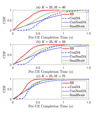
Figure 2: Comparison of the proposed scheme with baseline schemes.

Fig. 2 compares the completion time per UE of the proposed session-based (SB) scheme to those of the conventional data size-aware (ConDA), non-data size-aware (ConNoDA) schemes, and heuristic scheme on the small-scale fading time scale (SmallScale). The results in Fig. 2 are obtained using $200$ channels. The maximum completion time of UEs of ConNoDA is smaller than $\widetilde{T}_{c}$ and the minimum is larger than $T_{c}$. As seen, in terms of $90\%$-likely performance, the session-based scheme significantly outperforms ConDA, ConNoDA, and SmallScale when $M/K$ is small. Specifically, the $90\%$-likely completion time per UE of SB with $K=25,M=40$ is $0.48$s, which is $2-3$ times smaller than those of SmallScale, ConDA and ConNoDA. For the case of $(K=25,M=75)$ where $M/K$ is already large, the inter-user interference is relatively small, and hence, the improvement by our session-based scheme becomes smaller. The baseline schemes can outperform the proposed scheme in some cases but only in terms of less-than-$25\%$-likely performance. Fig. 2 also shows the advantage of joint optimization of user assignment, time, and rates over the small-scale allocation approach.

VI Conclusion

In this work, we have proposed a session-based scheme for the massive MIMO downlink, where the BS knows, a priori, the amount of data sent to the UEs. We formulated an optimization problem for assigning UEs to sessions and allocating power to minimize the completion time of the UEs. Utilizing successive convex approximation techniques, we proposed a novel algorithm to solve the formulated problem. Numerical results showed that our session-based scheme can significantly reduce the completion time compared with conventional schemes.

The proof basically follows the arguments in [9] with some modifications for our setting. Denote by $\operatorname{\mathcal{L}}_{\lambda}$ the optimal value of problem (24) corresponding to $\lambda$. Also, denote by $q^{*}$ the optimal value of problem (23). Then $q^{*}<+\infty$ due to the compactness of $\operatorname{\mathcal{F}}$. By a duality gap between the optimal values of problem (23) and its dual problem,

$$\sup_{\lambda\geq 0}\operatorname{\mathcal{L}}_{\lambda} =\sup_{\lambda\geq 0}\min_{\widetilde{\operatorname{\boldsymbol{x}}}\in\widehat{\operatorname{\mathcal{F}}}}\operatorname{\mathcal{L}}(\operatorname{\boldsymbol{a}},\tilde{\operatorname{\boldsymbol{r}}},\tilde{\operatorname{\boldsymbol{t}}},\operatorname{\boldsymbol{S}})\leq q^{*}=\min_{\widetilde{\operatorname{\boldsymbol{x}}}\in\widehat{\operatorname{\mathcal{F}}}}\max_{\lambda\geq 0}\operatorname{\mathcal{L}}(\operatorname{\boldsymbol{a}},\tilde{\operatorname{\boldsymbol{r}}},\tilde{\operatorname{\boldsymbol{t}}},\operatorname{\boldsymbol{S}}).$$

It follows that, for all $\lambda\geq 0$,

$$\operatorname{\mathcal{L}}_{\lambda}\leq q^{*}<+\infty.$$ (38)

For each $\lambda\geq 0$, let $V_{1,\lambda}\triangleq\sum_{k\in\operatorname{\mathcal{K}}}\sum_{i\in\operatorname{\mathcal{K}}}((\tilde{r}_{k,i})_{\lambda}(\tilde{t}_{k,i})_{\lambda}-(S_{k,i})_{\lambda})$ and $V_{2,\lambda}\triangleq\sum_{k\in\operatorname{\mathcal{N}}}\sum_{i\in\operatorname{\mathcal{K}}}((a_{k,i})_{\lambda}-(a_{k,i})_{\lambda}^{2}))$ be the values of $V_{1}$ and $V_{2}$ at the optimal solution $(\operatorname{\boldsymbol{a}}_{\lambda},\tilde{\operatorname{\boldsymbol{r}}}_{\lambda},\tilde{\operatorname{\boldsymbol{t}}}_{\lambda},\operatorname{\boldsymbol{S}}_{\lambda})$ of (24) corresponding to $\lambda$. We see from (14)–(18) that $V_{1,\lambda}\geq 0$ and from (22) that $V_{2,\lambda}\geq 0$. Set $V_{\lambda}\triangleq\gamma_{1}V_{1,\lambda}+\gamma_{2}V_{2,\lambda}$ and let $q_{\lambda}$ be the value of $q$ corresponding to $\lambda$. Next, let $0\leq\lambda_{1}<\lambda_{2}$. By the definition of $\operatorname{\mathcal{L}}_{\lambda_{1}}$ and $\operatorname{\mathcal{L}}_{\lambda_{2}}$,

$$\operatorname{\mathcal{L}}_{\lambda_{1}}=q_{\lambda_{1}}+\lambda_{1}V_{\lambda_{1}}\leq q_{\lambda_{2}}+\lambda_{1}V_{\lambda_{2}},$$ (39)

$$\operatorname{\mathcal{L}}_{\lambda_{2}}=q_{\lambda_{2}}+\lambda_{2}V_{\lambda_{2}}\leq q_{\lambda_{1}}+\lambda_{2}V_{\lambda_{1}},$$ (40)

from which we have $\lambda_{1}V_{\lambda_{1}}+\lambda_{2}V_{\lambda_{2}}\leq\lambda_{1}V_{\lambda_{2}}+\lambda_{2}V_{\lambda_{1}}$, and so $V_{\lambda_{2}}\leq V_{\lambda_{1}}$. This means $V_{\lambda}$ is decreasing as $\lambda$ is increasing. Since $V_{\lambda}=\gamma_{1}V_{1,\lambda}+\gamma_{2}V_{2,\lambda}\geq 0$ for all $\lambda\geq 0$, we obtain that $V_{\lambda}\rightarrow V^{*}\geq 0\text{~{}as~{}}\lambda\rightarrow+\infty$. From (39) and (40), we also have that $\lambda_{2}q_{\lambda_{1}}+\lambda_{1}q_{\lambda_{2}}\leq\lambda_{2}q_{\lambda_{2}}+\lambda_{1}q_{\lambda_{1}}$, which yields $q_{\lambda_{2}}\geq q_{\lambda_{1}}$. Therefore, as $\lambda\rightarrow+\infty$, $q_{\lambda}$ is increasing and hence bounded from below. Now, if $V^{*}>0$, then $\operatorname{\mathcal{L}}_{\lambda}=q_{\lambda}+\lambda V_{\lambda}\rightarrow+\infty$ as $\lambda\rightarrow+\infty$, which contradicts (38). Thus, we must have $V^{*}=0$, that is, $V_{\lambda}\rightarrow 0$ as $\lambda\rightarrow+\infty$, which implies that $V_{1,\lambda}\rightarrow 0$ and $V_{2,\lambda}\rightarrow 0$ as $\lambda\rightarrow+\infty$.

Finally, let $\widetilde{\operatorname{\boldsymbol{x}}}_{\lambda}$ be the value of $\widetilde{\operatorname{\boldsymbol{x}}}$ corresponding to $\lambda$. Then $\widetilde{\operatorname{\boldsymbol{x}}}_{\lambda}\in\widehat{\operatorname{\mathcal{F}}}$. Since $\widehat{\operatorname{\mathcal{F}}}$ is bounded, there exists a cluster point $\widetilde{\operatorname{\boldsymbol{x}}}_{*}$ of $\{\widetilde{\operatorname{\boldsymbol{x}}}_{\lambda}\}_{\lambda}$ as $\lambda\rightarrow+\infty$. We assume, without loss of generality, that $\widetilde{\operatorname{\boldsymbol{x}}}_{\lambda}\rightarrow\widetilde{\operatorname{\boldsymbol{x}}}_{*}$. Then, $\operatorname{\boldsymbol{a}}_{\lambda}\rightarrow\operatorname{\boldsymbol{a}}_{*}$, $\tilde{\operatorname{\boldsymbol{r}}}_{\lambda}\rightarrow\tilde{\operatorname{\boldsymbol{r}}}_{*}$, $\operatorname{\boldsymbol{S}}_{\lambda}\rightarrow\operatorname{\boldsymbol{S}}_{*}$, and $\tilde{\operatorname{\boldsymbol{t}}}_{\lambda}\rightarrow\tilde{\operatorname{\boldsymbol{t}}}_{*}$. It follows that $V_{1,\lambda}\rightarrow(V_{1})_{*}\!\triangleq\!\sum_{k\in\operatorname{\mathcal{K}}}\sum_{i\in\operatorname{\mathcal{K}}}((\tilde{r}_{k,i})_{*}(\tilde{t}_{k,i})_{*}-(S_{k,i})_{*})$, $V_{2,\lambda}\rightarrow(V_{2})_{*}\!\triangleq\!\sum_{k\in\operatorname{\mathcal{N}}}\sum_{i\in\operatorname{\mathcal{K}}}((a_{k,i})_{*}-(a_{k,i})_{*}^{2}))$, $V_{\lambda}\rightarrow V_{*}\triangleq\gamma_{1}(V_{1})_{*}+\gamma_{2}(V_{2})_{*}$, and $q_{\lambda}\rightarrow q_{*}$. As shown above, $(V_{1})_{*}=0$, $(V_{2})_{*}=0$, and $V_{*}=0$. Therefore, $(\tilde{\operatorname{\boldsymbol{r}}}_{*},\tilde{\operatorname{\boldsymbol{t}}}_{*},\operatorname{\boldsymbol{S}}_{*})$ and $(\operatorname{\boldsymbol{a}}_{*})$ satisfy (20) and (21), respectively. This together with $\widetilde{\operatorname{\boldsymbol{x}}}_{*}\in\widehat{\operatorname{\mathcal{F}}}$ implies that $\widetilde{\operatorname{\boldsymbol{x}}}_{*}\in\operatorname{\mathcal{F}}$, and so $\widetilde{\operatorname{\boldsymbol{x}}}_{*}$ is a feasible point of (23). As such, $q_{*}\geq q^{*}$. Next, the definition of $\operatorname{\mathcal{L}}_{\lambda}$ implies that, for all $\lambda\geq 0$, $\sup_{\lambda\geq 0}\operatorname{\mathcal{L}}_{\lambda}\geq\operatorname{\mathcal{L}}_{\lambda}=q_{\lambda}+\lambda V_{\lambda}\geq q_{\lambda}$. By letting $\lambda\rightarrow+\infty$, $\sup_{\lambda\geq 0}\operatorname{\mathcal{L}}_{\lambda}\geq q_{*}\geq q^{*}$. Combining with (38), yields $\sup_{\lambda\geq 0}\widetilde{\operatorname{\mathcal{L}}}(\lambda)=q_{*}=q^{*}$. We conclude that (25) holds and that $\widetilde{\operatorname{\boldsymbol{x}}}_{*}$ is an optimal solution of (23), which completes the proof.

References

• [1] N. Alexander et al., “The future of livestreaming: Strategy and predictive analysis for future operations of facebook live,” in Prof. IEEE SIEDS, Apr. 2021, pp. 1–6.
• [2] L. De Cicco and S. Mascolo, “An adaptive video streaming control system: Modeling, validation, and performance evaluation,” IEEE/ACM Transactions on Networking, vol. 22, no. 2, pp. 526–539, Apr. 2014.
• [3] T. T. Vu et al., “Cell-free massive MIMO for wireless federated learning,” IEEE Trans. Wireless Commun., vol. 19, no. 10, pp. 6377–6392, Oct. 2020.
• [4] H. Yan et al., “Discovering usage patterns of mobile video service in the cellular networks,” IEEE Trans. Netw. Serv. Manag., vol. 18, no. 2, pp. 1789–1802, Jun. 2021.
• [5] T. L. Marzetta, E. G. Larsson, H. Yang, and H. Q. Ngo, Fundamentals of Massive MIMO.   Cambridge University Press, 2016.
• [6] Y. Liu and E. Erkip, “Completion time in two-user channels: An information-theoretic perspective,” IEEE Trans. Inf. Theory, vol. 63, no. 5, pp. 3209–3223, May 2017.
• [7] T. T. Vu et al., “Energy-efficient massive MIMO for federated learning: Transmission designs and resource allocations,” Dec. 2021. [Online]. Available: https://arxiv.org/abs/2112.11723
• [8] M. Feng, M. Krunz, and W. Zhang, “Joint task partitioning and user association for latency minimization in mobile edge computing networks,” IEEE Trans. Veh. Technol., vol. 70, no. 8, pp. 8108–8121, Aug. 2021.
• [9] T. T. Vu et al., “Spectral and energy efficiency maximization for content-centric C-RANs with edge caching,” IEEE Trans. Commun., vol. 66, no. 12, pp. 6628–6642, Dec. 2018.
• [10] L. D. Nguyen et al., “Energy-efficient multi-cell massive MIMO subject to minimum user-rate constraints,” IEEE Trans. Commun., vol. 69, no. 2, pp. 914–928, Feb. 2021.
• [11] B. R. Marks and G. P. Wright, “A general inner approximation algorithm for nonconvex mathematical programs,” Operations Research, vol. 26, no. 4, pp. 681–683, Aug. 1978.
• [12] Further Advancements for E-UTRA Physical Layer Aspects (Release 9), document TS 36.814, 3GPP, Mar. 2010.