Stochastic gravitational waves from long cosmic strings

Abstract

We compute the expected strain power spectrum and energy density parameter of the stochastic gravitational wave background (SGWB) created by a network of long cosmic strings evolving during the whole cosmic history. As opposed to other studies, the contribution of cosmic string loops is discarded and our result provides a robust lower bound of the expected signal that is applicable to most string models. Our approach uses Nambu-Goto numerical simulations, running during the radiation, transition and matter eras, in which we compute the two-point unequal-time anisotropic stress correlators. These ones act as source terms in the linearised equations of motion for the tensor modes, that we solve using an exact Green’s function integrator. Today, we find that the rescaled strain power spectrum $(k/\mathcal{H}_{0})^{2}\mathcal{P}_{h}$ peaks on Hubble scales and exhibits, at large wavenumbers, high frequency oscillations around a plateau of amplitude $100(GU)^{2}$. Most of the high frequency power is generated by the long strings present in the matter era, the radiation era contribution being smaller.

1 Introduction

The advent of gravitational wave astronomy has triggered a renewed interest in the search for cosmic strings [1, 2, 3, 4, 5, 6, 7, 8, 9, 10]. These objects can be of diverse cosmological origins, ranging from topological defects formed during phase transitions in the Early Universe [11, 12, 13] to fundamental strings living in higher warped multi-dimensional spaces [14, 15, 16, 17].

Cosmic strings have been actively searched in various astronomical and cosmological observables, for almost forty years, without triggering any confirmed detection, see, e.g., Refs. [18, 19, 20, 21, 22, 23, 24, 25, 26, 27, 28, 29, 30, 31]. As of today, the strongest bound on the most detectable strings comes from the stochastic gravitational wave background limits set by the laser interferometers in the tens of Hertz frequency window [32, 33]. They report a maximal energy scale for cosmic strings around $10^{12}\,\mathrm{GeV}$. Such an upper bound is remarkably low, it deeply probes the energy scales that would be associated with symmetry breaking occurring in the Grand Unified Theories. At the same time, there is plenty of room for strings to be formed at lower energies while a non-vanishing SGWB has been reported in the nano-Hertz range [34, 35]. Moreover, the aforementioned limit only applies to Nambu-Goto cosmic string loops having sizes given by the Polchinski-Rocha scaling distribution [36, 37, 38, 39], which, in addition, are assumed to have a microstructure filled with “kinks”. Kinks are light-like moving shocks in the shape of the strings that repeatedly collide and create spherical bursts of gravitational waves [40, 41]. The actual microstucture of loops [42, 43, 44] and the shape of their number density distribution at small length scales are still a matter of discussion [36, 45, 39, 46, 47, 48]. This is particularly relevant as tiny changes in these quantities have been shown to significantly impact the resulting gravitational wave signal [40, 49]. Furthermore, the distribution of loops may be model-dependent, and, at one extreme end, cosmic strings made of Abelian Higgs field are observed to not produce stable loops at all [50, 51]. In this situation, only the long strings in a network would create persistent observable signatures and are constrained by their effects onto the Cosmic Microwave Background (CMB). The maximal possible energy scale compatible with the Planck satellite data [52] is around $10^{15}\,\mathrm{GeV}$ [30, 53, 54, 55, 56, 57, 58]. Let us mention that a non-scaling cosmic string network, as one that would be formed during inflation, is even less constrained [59, 60, 61, 62, 63, 64]. Such a model dependence can nevertheless be a virtue as more complex strings, e.g., the ones endowed with currents, can potentially be detected via other means than gravitational effects [65, 66, 67, 68, 69, 70, 71, 72, 73, 74].

In this paper, we focus on the stochastic gravitational wave background produced by the long strings only, assuming that they are the backbones of a scaling network. In order to consider most realistic strings, we have performed new Nambu-Goto numerical simulations, based on a modern version of the Bennett-Bouchet code [75, 76, 30, 54], in the radiation and matter eras, as well as during the transition from radiation to matter. While in scaling, a Nambu-Goto cosmic string network exhibits universal statistical properties and any observable quantity depends only on one dimensionless parameter $GU$, where $U$ is the string energy density, equals to the string tension, and $G$ the Newton constant [77]. The Nambu-Goto simulations allow us to compute, without any approximation, the stress tensor associated with the long strings, from which we derive the unequal-time two-point correlators (UETC) of the anisotropic stress. These correlators act as source terms in the linearised equations of motion for the spin-two fluctuations propagating around a Friedmann-Lemaître-Robertson Walker metric [78, 79, 80, 81]. The method is inspired from the one presented in Refs. [82, 83], which has, up to now, only been applied to global defects. However, as we discuss below, we have paid special attention to keep all time and length scale dependence in the computed waveforms in order to not wash-out any oscillatory fine structure. This is particularly relevant in view of the results derived in Ref. [84], which suggest that cosmic strings would behave as “singular” sources at high frequencies. In the following, we confirm these analytic expectations while providing accurate numerical results for the overall shape of the gravitational wave spectra. In particular, we find that the strain power spectrum at large wavenumbers is driven by the long strings evolving in the matter era, the contribution of the radiation-era strings being a few orders of magnitude smaller.

The paper is organised as follows. In section 2, we give some mathematical details on the Green’s function method used to compute the spectra from the UETC while discussing the accuracy of assuming a pure radiation, or matter, era instead of the $\Lambda$CDM solution. In section 3, we give some details on the Nambu-Goto numerical simulations and the method used to compute the UETC while ensuring that they are close to the scaling regime. Finally, in section 4, we present our main results, which are the SGWB spectra of the rescaled strain $k^{2}/(12\mathcal{H}_{0}^{2})\mathcal{P}_{h}(k)$, and the energy density parameter $\Omega_{\mathrm{gw}}(k)$, generated by long cosmic strings. Finally, we conclude in section 5.

2 Gravitational waves of cosmological origin

In this section, we briefly recap the linearised equations for the tensor modes created and propagated in a Friedmann-Lemaître-Robertson-Walker (FLRW) metric. We then discuss the computation of the associated Green’s function in the $\Lambda$CDM model.

2.1 Linearised equations of motion

Assuming a spatially flat metric of the form

$$\mathrm{d}s^{2}=a^{2}(\eta)\left\{-\mathrm{d}\eta^{2}+\left[\delta_{ij}+h_{ij}(\eta,{\boldsymbol{x}})\right]\mathrm{d}x^{i}\mathrm{d}x^{j}\right\},$$ (2.1)

where $h_{ij}(\eta,{\boldsymbol{x}})$ is a gauge-invariant divergenceless and traceless tensor (Roman indices running only on spatial dimensions), the Einstein equations, linearised at first order in $h_{ij}$, read

$$h_{ij}^{\prime\prime}+2\dfrac{a^{\prime}}{a}h_{ij}^{\prime}-\Delta h_{ij}=\dfrac{2}{M_{\mathrm{Pl}}^{2}}a^{2}\varPi_{ij}.$$ (2.2)

Here a prime denotes differentiation with respect to $\eta$, the conformal time, the Laplacian operator is over the comoving spatial coordinates ${\boldsymbol{x}}$ and $M_{\mathrm{Pl}}$ stands for the reduced Planck mass. The source term $\varPi_{ij}=\delta T_{ij}^{\mathrm{{\scriptscriptstyle{TT}}}}(\eta,{\boldsymbol{x}})/a^{2}$ is the traceless and transverse anisotropic part of the linearised stress tensor $\delta T_{\mu\nu}$ at the origin of the perturbations [85]. In these equations, all scalars and vectors have been assumed to vanish as we are only focused in the generation and propagation of gravitational waves. In order to solve equation (2.2) in the presence of long cosmic strings, we need to compute $\varPi_{ij}(\eta,{\boldsymbol{x}})$ and invert the differential operator to get $h_{ij}(\eta,{\boldsymbol{x}})$. Moreover, we are interested in the statistical properties of the stochastic background generated by the superimposition of all these waves and one has to construct the two-point correlation functions of these quantities.

In the helicity basis, and Fourier space, the strain can be decomposed as [86, 87]

$$h_{ij}(\eta,{\boldsymbol{x}})=\dfrac{1}{(2\pi)^{3}}\int_{-\infty}^{\infty}\sum_{r=-2,+2}h_{r}(\eta,{\boldsymbol{k}})\epsilon_{ij}^{r}({\boldsymbol{e}}_{k})e^{\imath{\boldsymbol{k}}{\boldsymbol{x}}}\mathrm{d}^{3}{\boldsymbol{k}},$$ (2.3)

where the $\epsilon_{ij}^{r}({\boldsymbol{e}}_{k})$ are the component of the helicity basis tensor. In the Fourier spherical coordinate system $({\boldsymbol{e}}_{k},{\boldsymbol{e}}_{1},{\boldsymbol{e}}_{2})$, they read

$${\boldsymbol{\epsilon}}^{\pm 2}=\dfrac{1}{2}\left({\boldsymbol{e}}_{1}\pm\imath{\boldsymbol{e}}_{2}\right)\otimes\left({\boldsymbol{e}}_{1}\pm\imath{\boldsymbol{e}}_{2}\right),$$ (2.4)

and verifies

$$\epsilon_{ij}^{r*}\epsilon^{ij}_{s}=\delta^{r}_{s}.$$ (2.5)

Moreover, one has the relation $\epsilon_{ij}^{\pm 2}(-{\boldsymbol{e}}_{k})=\epsilon_{ij}^{\pm 2*}({\boldsymbol{e}}_{k})$ to ensure that $h_{ij}(\eta,{\boldsymbol{x}})$ are real quantities. In the following, we will work with the mode function

$$\mu_{r}\equiv a(\eta)h_{r},$$ (2.6)

which, from equation (2.2), is solution of

$$\mu_{r}^{\prime\prime}(\eta,{\boldsymbol{k}})+\left(k^{2}-\dfrac{a^{\prime\prime}}{a}\right)\mu_{r}(\eta,{\boldsymbol{k}})=\dfrac{2}{M_{\mathrm{Pl}}^{2}}a^{3}\varPi_{r}(\eta,{\boldsymbol{k}}).$$ (2.7)

This equation can be exactly solved using the retarded Green’s function, $G_{\xi}(\eta,{\boldsymbol{k}})$, solution of the same equation with a source term distribution in $\delta(\eta-\xi)$. Assuming $G_{\xi}(\eta,{\boldsymbol{k}})$ to be known, and the source $\varPi_{r}$ to vanish at times $\eta<\eta_{\mathrm{ini}}$, the mode function, and its time derivative, are then given by

$$\mu_{r}(\eta,{\boldsymbol{k}}) =\dfrac{2}{M_{\mathrm{Pl}}^{2}k}\int_{\eta_{\mathrm{ini}}}^{\eta}kG_{\xi}(\eta,k)a^{3}(\xi)\varPi_{r}(\xi,{\boldsymbol{k}})\mathrm{d}\xi,$$ (2.8)

$$\mu_{r}^{\prime}(\eta,{\boldsymbol{k}}) =\dfrac{2}{M_{\mathrm{Pl}}^{2}}\int_{\eta_{\mathrm{ini}}}^{\eta}G_{\xi}^{\prime}(\eta,k)a^{3}(\xi)\varPi_{r}(\xi,{\boldsymbol{k}})\mathrm{d}\xi.$$

where $G_{\xi}^{\prime}$ stands for $\partial G_{\xi}(\eta,k)/\partial\eta$. Notice that these equations encode both the generation of gravitational waves, in the domains for which $\varPi_{r}(\xi,{\boldsymbol{k}})\neq 0$, and the propagation to the observer thanks to the Green’s functions. We now turn to the determination of these functions.

2.2 Computation of the Green’s functions

There are known analytical solutions for the retarded Green’s functions associated with equation (2.7) and we simply quote the results. If the scale factor behaves as in a pure radiation era $a(\eta)\propto\eta$, one has [88]

$$kG^{\mathrm{rad}}_{\xi}(\eta,k)=\sin\left[k(\eta-\xi)\right]\mathrm{\Theta}\!\left(\eta-\xi\right).$$ (2.9)

For a matter era that instantaneously succeeds the radiation era one has $a(\eta)\propto(\eta+\eta_{\mathrm{eq}})^{2}$ and [84]

$$kG^{\mathrm{mat}}_{\xi}(\eta,k) =\left\{\sin\left[k(\eta-\xi)\right]-\dfrac{k(\eta-\xi)}{k(\eta+\eta_{\mathrm{eq}})\,k(\xi+\eta_{\mathrm{eq}})}\cos\left[k(\eta-\xi)\right]\right.$$ (2.10)

$$\left.+\dfrac{1}{k(\eta+\eta_{\mathrm{eq}})\,k(\xi+\eta_{\mathrm{eq}})}\sin\left[k(\eta-\xi)\right]\right\}\mathrm{\Theta}\!\left(\eta-\xi\right).$$

Let us stress that, in this last expression, $\eta_{\mathrm{eq}}$ is not a free parameter. Denoting by $\mathcal{H}_{0}=\mathcal{H}(\eta_{0})$ the conformal Hubble parameter today, it is defined as [84]

$$\eta_{\mathrm{eq}}\equiv\dfrac{\sqrt{\Omega_{\mathrm{rad}}}}{\mathcal{H}_{0}\Omega_{\mathrm{mat}}}\,,$$ (2.11)

to ensure continuity of the scale factor, and its derivative, at the instantaneous transition between radiation and matter. In particular, its numerical value differs (by a few) from the conformal time at which there would be the actual equality between the energy density of matter and radiation.

The evolution of the scale factor $a(\eta)$ in presence of a mixture of radiation and matter can be exactly solved from the Friedmann-Lemaître equations and reads

$$a(\eta)=\dfrac{\Omega_{\mathrm{mat}}\mathcal{H}_{0}^{2}}{4}\eta^{2}+\sqrt{\Omega_{\mathrm{rad}}}\mathcal{H}_{0}\eta.$$ (2.12)

Plugging this expression into equation (2.7), the associated Green’s function $G^{\mathrm{mix}}_{\xi}(\eta,k)$ is solution of

$$\dfrac{\mathrm{d}^{2}\left[kG^{\mathrm{mix}}_{y}(x)\right]}{\mathrm{d}x^{2}}+\left(1-\dfrac{2}{x^{2}+4x_{\mathrm{eq}}x}\right)kG^{\mathrm{mix}}_{y}(x)=\delta(x-y),$$ (2.13)

where we have made the change of variables

$$x\equiv k\eta,\qquad y=k\xi,\qquad x_{\mathrm{eq}}=k\eta_{\mathrm{eq}}\,.$$ (2.14)

In spite of a simple form, equation (2.13) has no analytic solutions and must be solved numerically. Using the Wronskian method, for each value of $x$ and $y$, one needs two numerical integrations, with different initial conditions, to allow for the determination of the Green’s function. These solutions are represented in figures 1 and 2, where they are compared to the approximations given by equations (2.9) and (2.10) as well as to the $\Lambda$CDM solution (see below).

We have also numerically determined the Green’s function $kG^{\mathrm{lcdm}}_{\xi}(\eta,k)$, that we refer to as “exact” in these figures. It is obtained by considering the scale factor evolution associated with the $\Lambda$CDM model, the cosmological parameter values having being fixed to the ones favoured by the Planck satellite measurements [89]. In this situation, there is no analytical solution for the scale factor evolution $a(\eta)$. The determination of $kG^{\mathrm{lcdm}}_{\xi}(\eta,k)$, at fixed $\xi$, $\eta$ and $k$, therefore requires, in parallel to the two aforementioned numerical integrations, the computation of $a^{\prime\prime}(\eta)/a(\eta)$ appearing in equation (2.7). This one is obtained by numerically integrating the Friedmann-Lemaître equations.

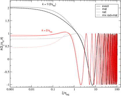
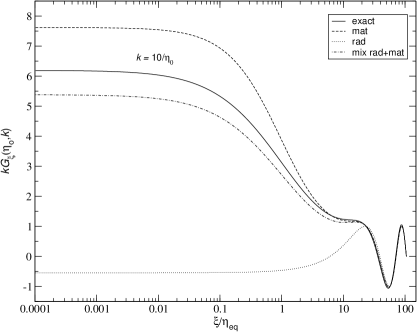
Figure 1: Green’s functions $kG_{\xi}(\eta=\eta_{0},k)$ associated with the evolution of tensor modes, up to now. They are plotted for various values of the wavenumber $k$, as a function of the time parameter $\xi$, expressed in unit of $\eta_{\mathrm{eq}}$. The right-most value of $\xi/\eta_{\mathrm{eq}}\simeq 105$ corresponds to today with $\xi=\eta_{0}$. The label “exact” stands for the Green’s function computed for the $\Lambda$CDM model while “rad+mat” for a scale factor driven by a mixture of radiation and matter. The labels “rad” and “mat” refer to the analytical solutions obtained by assuming a pure radiation era, and, a matter era patched to a radiation era, given by equations (2.9) and (2.10), respectively. The most commonly used approximation in the literature (“rad”) always produces erroneous values at early times. It remains acceptable only on the time domains for which the mode remains deeply sub-Hubbles (see also figure 2). On the contrary, the matter era solution is surprisingly good, even during the radiation era.

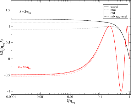
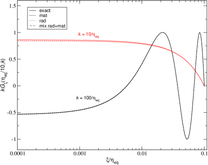
Figure 2: The Green’s function $kG_{\xi}(\eta_{\mathrm{eq}},k)$ (left panel) and $kG_{\xi}(\eta_{\mathrm{eq}}/10,k)$ (right panel), evaluated for a time parameter $\xi$ exploring the radiation era. As one may expect, the Green’s function computed for a mixture of radiation and matter is undistinguishable from the exact one. However, for $\eta$ set at the transition (left plot), the matter era Green’s function is still a better approximation than the one derived assuming pure radiation. Deeper into the radiation era, at $\eta=\eta_{\mathrm{eq}}/10$ (right plot), all approximations are undistinguishable from the exact solution.

In figure 1, we have represented the Green’s functions $kG_{\xi}(\eta,k)$, evaluated at the present time $\eta=\eta_{0}$, for various values of $k$, as a function of the time parameter $\xi$. As can be seen in equation (2.8), once multiplied by the anisotropic stress, this is the quantity of interest to perform the convolution integral. The left panel shows two modes entering the Hubble radius around equality, $k=1/(2\eta_{\mathrm{eq}})$ (black curves) and $k=2/\eta_{\mathrm{eq}}$ (red curves). For each of them, we have plotted the numerical $\Lambda$CDM solution (labelled “exact”), the numerical solution of equation (2.13) (“rad+mat”), equation (2.9) (“rad”) and equation (2.10) (“mat”). In most of the matter era ($\xi/\eta_{\mathrm{eq}}\gg 1$), the modes are sub-Hubble and freely propagate, all Green’s functions are the same. However, at earlier times, when the modes were of wavelength close, or greater, than the Hubble radius at that time (for $\xi/\eta_{\mathrm{eq}}\lesssim 1$), deviations appear. The differences between $G^{\mathrm{lcdm}}_{\xi}$ and $G^{\mathrm{mix}}_{\xi}$ are barely visible whereas the pure radiation era Green’s function $G^{\mathrm{rad}}_{\xi}$ is the most inaccurate. For the mode $k=1/(2\eta_{\mathrm{eq}})$, differences between $G^{\mathrm{rad}}_{\xi}$ and the others are noticeable for $\xi/\eta_{\mathrm{eq}}\lesssim 10$. Interestingly, $G^{\mathrm{mat}}_{\xi}$ remains a relatively good approximation of the exact solution even for the super-Hubble modes in the radiation era. The right panel of figure 1 shows the Green’s functions for a mode of wavelength close to the Hubble radius today, $k=10/\eta_{0}$. Differences between the exact solution $G^{\mathrm{lcdm}}_{\xi}$ and the mixture radiation and matter $G^{\mathrm{mix}}_{\xi}$ are now visible. This is expected as the cosmological constant domination is very recent in the history of the Universe and can only show up at time $\eta\simeq\eta_{0}$. The radiation era Green’s function still dramatically fails while the matter era one overestimates the expected values, up to $20\%$ in the radiation era.

It is important to notice that these conclusions are $\eta$-dependent. Therefore, in figure 2 we have represented the very same functions, $kG_{\xi}(\eta,k)$, but evaluated at times which are either during the transition $\eta=\eta_{\mathrm{eq}}$ (left panel), or during the radiation era at $\eta_{\mathrm{eq}}/10$ (right panel). The differences are less pronounced than for $\eta=\eta_{0}$, but, still, for all modes becoming super-Hubble close to $\xi=\eta_{\mathrm{eq}}$, $G^{\mathrm{rad}}_{\xi}$ differs from the others. Confined within the radiation era (right panel), all functions lead to the same values, including the matter era one.

In conclusion, using $G^{\mathrm{mix}}_{\xi}$ (mixture radiation and matter) to describe the generation and propagation of gravitational waves is accurate at all times and for all modes which are sub-Hubble today, namely $k>10/\eta_{0}$. Next in accuracy is, quite surprisingly, the fully analytic matter era Green’s function $G^{\mathrm{mat}}_{\xi}$ given by equation (2.10). It remains within a ten percent error margin from the exact solution, and mostly deviates for Hubble-like modes today, as expected from the present acceleration of the Universe which is not accounted for. The worse of all is $G^{\mathrm{rad}}_{\xi}$. It is accurate only for modes created, propagated and measured within the radiation era.

Let us finally notice that the accuracy of the final result, namely the value of $\mu_{r}(\eta,{\boldsymbol{k}})$, also depends on the support of the anisotropic stress $\varPi_{r}(\xi,{\boldsymbol{k}})$. If this one vanishes in the domains in which the Green’s function is inaccurate, the final result may very well be valid, but this is no trivial a priori and needs to be checked.

2.3 Propagating gravitational wave power spectra

The superimposition of all gravitational waves generated by a network of long cosmic strings produces a stochastic background, which is, at leading order, isotropic. Comparison with observation requires to determine its statistical properties, and, in this paper, we focus on the two-point correlation functions. In Fourier space, using the statistical invariance by translation, the unequal time correlator of the strain is of the form

$$\left\langle h_{r}^{*}(\eta_{1},{\boldsymbol{k}})h_{r}(\eta_{2},{\boldsymbol{q}})\right\rangle\equiv\dfrac{(2\pi)^{3}}{V}\delta\negthinspace\left({\boldsymbol{k}}-{\boldsymbol{q}}\right)P_{h_{r}}(\eta_{1},\eta_{2},{\boldsymbol{k}}),$$ (2.15)

where we have made the (infinite) volume factor $V$ explicit. Statistical isotropy implies that $P_{h_{r}}(\eta_{1},\eta_{2},{\boldsymbol{k}})=P_{h_{r}}(\eta_{1},\eta_{2},k)$ and the strain correlation function in real space can be expressed as

$$\left\langle h_{ij}(\eta_{1},{\boldsymbol{x}})h^{ij}(\eta_{2},{\boldsymbol{x}}+{\boldsymbol{y}})\right\rangle=\int_{0}^{\infty}\dfrac{\mathrm{d}q}{q}\mathcal{P}_{h}(\eta_{1},\eta_{2},q)\operatorname{sinc}(qy),$$ (2.16)

where the (spherical) strain power spectrum we are interested in reads

$$\mathcal{P}_{h}(\eta_{1},\eta_{2},k)=\sum_{r}\mathcal{P}_{h_{r}}(\eta_{1},\eta_{2},k)\equiv\dfrac{k^{3}V}{2\pi^{2}}\sum_{r}P_{h_{r}}(\eta_{1},\eta_{2},k).$$ (2.17)

Similarly, the spatial two-point correlators of the time derivative $h_{r}^{\prime}$ is expressed, in Fourier space, as the dimensionless parameter

$$\Omega_{\mathrm{gw}}(\eta_{1},\eta_{2},k)\equiv\dfrac{\sum_{r}\mathcal{P}_{h_{r}^{\prime}}(\eta_{1},\eta_{2},k)}{12\mathcal{H}(\eta_{1})\mathcal{H}(\eta_{2})}\,,$$ (2.18)

where $\mathcal{P}_{h_{r}^{\prime}}$ is defined from $P_{h_{r}^{\prime}}$ in the exact same manner as in equations (2.15) and (2.17).

From equations (2.6), both $P_{h_{r}}$ and $P_{h_{r}^{\prime}}$ can be derived from the power spectra of $\mu_{r}$ and $\mu_{r}^{\prime}$. One has [84]

$$P_{h_{r}}(\eta_{1},\eta_{2},k) =\dfrac{P_{\mu_{r}}(\eta_{1},\eta_{2},k)}{a(\eta_{1})a(\eta_{2})}\,,$$ (2.19)

$$P_{h_{r}^{\prime}}(\eta_{1},\eta_{2},k) =H(\eta_{1})H(\eta_{2})\left[\dfrac{P_{\mu_{r}^{\prime}}(\eta_{1},\eta_{2},k)}{\mathcal{H}(\eta_{1})\mathcal{H}(\eta_{2})}+P_{\mu_{r}}(\eta_{1},\eta_{2},k)-\dfrac{P_{\kappa_{r}}(\eta_{1},\eta_{2},k)}{\mathcal{H}(\eta_{1})}\right.$$

$$\left.-\dfrac{P_{\bar{\kappa}_{r}}(\eta_{1},\eta_{2},k)}{\mathcal{H}(\eta_{2})}\right].$$

where we have defined

$$\left\langle{\mu_{r}^{\prime}}^{*}(\eta_{1},{\boldsymbol{k}})\mu_{r}(\eta_{2},{\boldsymbol{q}})\right\rangle=\dfrac{(2\pi)^{3}}{V}\delta\negthinspace\left({\boldsymbol{k}}-{\boldsymbol{q}}\right)P_{\kappa_{r}}(\eta_{1},\eta_{2},{\boldsymbol{k}}),$$ (2.20)

and $P_{\bar{\kappa}_{r}}(\eta_{1},\eta_{2},{\boldsymbol{k}})=P_{\kappa_{r}}^{*}(\eta_{2},\eta_{1},{\boldsymbol{k}})$. From equation (2.8), one has

$$P_{\mu_{r}}(\eta_{1},\eta_{2},{\boldsymbol{k}}) =\dfrac{4}{k^{2}M_{\mathrm{Pl}}^{4}}\int_{\eta_{\mathrm{ini}}}^{\eta_{1}}\mathrm{d}\xi\int_{\eta_{\mathrm{ini}}}^{\eta_{2}}\mathrm{d}\xi^{\prime}kG_{\xi}^{*}(\eta_{1},k)\,kG_{\xi^{\prime}}(\eta_{2},k)a^{3}(\xi)a^{3}(\xi^{\prime})\left\langle\varPi_{r}^{*}(\xi,{\boldsymbol{k}})\varPi_{r}(\xi^{\prime},{\boldsymbol{k}})\right\rangle,$$ (2.21)

$$P_{\mu_{r}^{\prime}}(\eta_{1},\eta_{2},{\boldsymbol{k}}) =\dfrac{4}{M_{\mathrm{Pl}}^{4}}\int_{\eta_{\mathrm{ini}}}^{\eta_{1}}\mathrm{d}\xi\int_{\eta_{\mathrm{ini}}}^{\eta_{2}}\mathrm{d}\xi^{\prime}{G_{\xi}^{\prime}}^{*}(\eta_{1},k)G_{\xi^{\prime}}^{\prime}(\eta_{2},k)a^{3}(\xi)a^{3}(\xi^{\prime})\left\langle\varPi_{r}^{*}(\xi,{\boldsymbol{k}})\varPi_{r}(\xi^{\prime},{\boldsymbol{k}})\right\rangle,$$

$$P_{\kappa_{r}}(\eta_{1},\eta_{2},{\boldsymbol{k}}) =\dfrac{4}{kM_{\mathrm{Pl}}^{4}}\int_{\eta_{\mathrm{ini}}}^{\eta_{1}}\mathrm{d}\xi\int_{\eta_{\mathrm{ini}}}^{\eta_{2}}\mathrm{d}\xi^{\prime}{G_{\xi}^{\prime}}^{*}(\eta_{1},k)\,kG_{\xi^{\prime}}(\eta_{2},k)a^{3}(\xi)a^{3}(\xi^{\prime})\left\langle\varPi_{r}^{*}(\xi,{\boldsymbol{k}})\varPi_{r}(\xi^{\prime},{\boldsymbol{k}})\right\rangle.$$

As a result, the source terms needed to uniquely determine all the power spectra are the unequal time anisotropic stress correlators. Using translational invariance and statistical isotropy, they can be redefined as

$$\left\langle\varPi_{r}^{*}(\xi,{\boldsymbol{k}})\varPi_{r}(\xi^{\prime},{\boldsymbol{q}})\right\rangle=\dfrac{(2\pi)^{3}}{V}\delta\negthinspace\left({\boldsymbol{k}}-{\boldsymbol{q}}\right)\dfrac{U^{2}\mathcal{T}_{r}(\xi,\xi^{\prime},k)}{a^{2}(\xi)\sqrt{\xi}\,a^{2}(\xi^{\prime})\sqrt{\xi^{\prime}}}\,,$$ (2.22)

Here, we have explicitly factorised the typical energy density scale $U^{2}$ and $\mathcal{T}_{r}(\xi,\xi^{\prime},k)$ is a dimensionless function. The interest of expressing the anisotropic stress correlators as in equation (2.22) is that, when the source terms are in the so-called scaling regime, one has [81, 90, 91, 92]

$$\mathcal{T}_{r}(\xi,\xi^{\prime},k)=\mathcal{U}_{r}(k\xi,k\xi^{\prime}).$$ (2.23)

A network of cosmic strings reaches scaling in both the radiation and matter era, with, however, different functions, say, $\mathcal{U}^{\mathrm{rad}}_{r}(x,x^{\prime})$ and $\mathcal{U}^{\mathrm{mat}}_{r}(x,x^{\prime})$, where $x=k\eta$. Let us notice that equation (2.22) is valid even if the anisotropic stress does not assume a scaling form and we will be using $\mathcal{T}_{r}(\xi,\xi^{\prime},k)$ during the transition between the radiation and the matter eras.

Plugging equation (2.22) into equation (2.21), one can simplify equation (2.17) into

$$\mathcal{P}_{h}(\eta_{1},\eta_{2},k)=128(GU)^{2}I_{\mu}(x_{1},x_{2},k),$$ (2.24)

where the integral

$$I_{\mu}(x_{1},x_{2},k)\equiv\dfrac{1}{a(\eta_{1})a(\eta_{2})}\int_{x_{\mathrm{ini}}}^{x_{1}}\mathrm{d}x\int_{x_{\mathrm{ini}}}^{x_{2}}\mathrm{d}x^{\prime}K_{\mathrm{s}}(x_{1},x)K_{\mathrm{s}}(x_{2},x^{\prime})\dfrac{a\left(\frac{x}{k}\right)a\left(\frac{x^{\prime}}{k}\right)}{\sqrt{xx^{\prime}}}\mathcal{T}\left(\frac{x}{k},\frac{x^{\prime}}{k},k\right).$$ (2.25)

In this expression, we have defined the dimensionless parameters $x_{1}=k\eta_{1}$, $x_{2}=k\eta_{2}$ and $x_{\mathrm{ini}}=k\eta_{\mathrm{ini}}$ as well as $\mathcal{T}=\sum_{r}\mathcal{T}_{r}$. The integration kernel for the strain, $K_{\mathrm{s}}$, is the rescaled Green’s function, see equation (2.13), and reads

$$K_{\mathrm{s}}(x_{i},x)\equiv kG_{x}(x_{i}).$$ (2.26)

One can also express $\Omega_{\mathrm{gw}}$ in terms of similar integrals. From equations (2.18) and (2.21), one gets

$$\Omega_{\mathrm{gw}}(\eta_{1},\eta_{2},k) =\dfrac{32}{3}\left(GU\right)^{2}\left[\dfrac{k^{2}}{\mathcal{H}(\eta_{1})\mathcal{H}(\eta_{2})}I_{\mu^{\prime}}(x_{1},x_{2},k)+I_{\mu}(x_{1},x_{2},k)\right.$$ (2.27)

$$\left.-\dfrac{k}{\mathcal{H}(\eta_{1})}I_{\kappa}(x_{1},x_{2},k)-\dfrac{k}{\mathcal{H}(\eta_{2})}I_{\bar{\kappa}}(x_{1},x_{2},k)\right],$$

with

$$I_{\mu^{\prime}}(x_{1},x_{2},k) \equiv\dfrac{1}{a(\eta_{1})a(\eta_{2})}\int_{x_{\mathrm{ini}}}^{x_{1}}\mathrm{d}x\int_{x_{\mathrm{ini}}}^{x_{2}}\mathrm{d}x^{\prime}K_{\mathrm{e}}(x_{1},x)K_{\mathrm{e}}(x_{2},x^{\prime})\dfrac{a\left(\frac{x}{k}\right)a\left(\frac{x^{\prime}}{k}\right)}{\sqrt{xx^{\prime}}}\mathcal{T}\left(\frac{x}{k},\frac{x^{\prime}}{k},k\right),$$ (2.28)

$$I_{\kappa}(x_{1},x_{2},k) \equiv\dfrac{1}{a(\eta_{1})a(\eta_{2})}\int_{x_{\mathrm{ini}}}^{x_{1}}\mathrm{d}x\int_{x_{\mathrm{ini}}}^{x_{2}}\mathrm{d}x^{\prime}K_{\mathrm{e}}(x_{1},x)K_{\mathrm{s}}(x_{2},x^{\prime})\dfrac{a\left(\frac{x}{k}\right)a\left(\frac{x^{\prime}}{k}\right)}{\sqrt{xx^{\prime}}}\mathcal{T}\left(\frac{x}{k},\frac{x^{\prime}}{k},k\right),$$

and $I_{\bar{\kappa}}(x_{1},x_{2},k)=I_{\kappa}^{*}(x_{2},x_{1},k)$. In these two integrals, the energy kernel, $K_{\mathrm{e}}$, is defined as

$$K_{\mathrm{e}}(x_{i},x)\equiv\left.\dfrac{\partial\left[kG_{x}(y)\right]}{\partial y}\right|_{y=x_{i}}=\dfrac{\partial K_{\mathrm{s}}(x_{i},x)}{\partial x_{i}}\,.$$ (2.29)

As a result, we have the following relations

$$I_{\mu^{\prime}}(x_{1},x_{2},k)=\dfrac{\partial^{2}I_{\mu}(x_{1},x_{2},k)}{\partial x_{1}\partial x_{2}}\,,\qquad I_{\kappa}(x_{1},x_{2},k)=\dfrac{\partial I_{\mu}(x_{1},x_{2},k)}{\partial x_{1}}\,,$$ (2.30)

and, a priori, only $I_{\mu}(x_{1},x_{2},k)$ needs to be determined for computing both $\mathcal{P}_{h}$ and $\Omega_{\mathrm{gw}}$. However, in the absence of an analytical expression for $I_{\mu}$, it is easier and more accurate to compute the three integrals $I_{\mu}$, $I_{\mu^{\prime}}$ and $I_{\kappa}$ separately. The integration kernels $K_{\mathrm{s}}$ and $K_{\mathrm{e}}$ being the Green’s function of $\mu$ and $\mu^{\prime}$, their determination has already been discussed in section 2.2. In the next section, we present the method used to numerically estimate the function $\mathcal{T}$.

3 Anisotropic stress correlators

3.1 Nambu-Goto numerical simulations

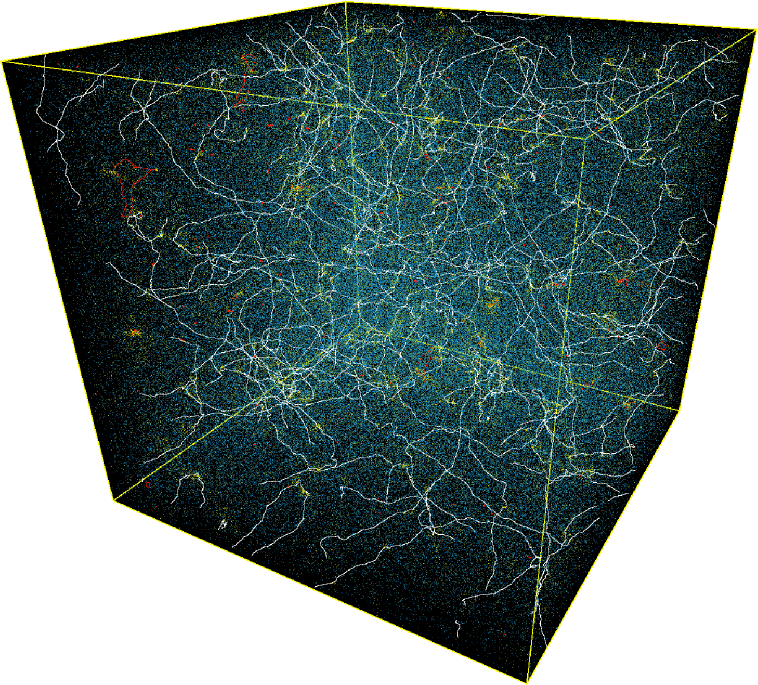
Figure 3: Snapshot of the cosmic string network during the transition era when the conformal horizon occupies $60\%$ of the fixed comoving volume $(100l_{\mathrm{c}})^{3}$. For this work, the stress tensor includes only the contribution of the long strings, defined as being longer than the horizon size. They are represented in white in the picture. Loops in scaling are represented in red whereas freshly formed loops coming from the fragmentation of larger structures are represented in yellow. The blue “fog” is made of tiny older loops. There are about two million strings in this picture, they are all numerically evolved till the end of the run.

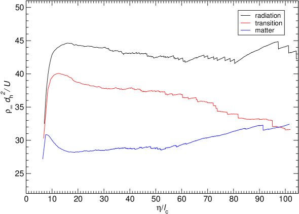
Figure 4: Rescaled energy density of the long strings, defined as being longer than the horizon size, as a function of the simulation conformal time $\eta$ (in unit of the initial correlation length $l_{\mathrm{c}}$). The curves correspond to the three runs made in the radiation, transition and matter era. After a fast growing phase for $\eta\simeq d_{\mathrm{h}_{\mathrm{i}}}$ (leftmost side), the long strings reach a scaling regime during which $\rho_{\infty}d_{\mathrm{h}}^{2}$ remains stationary. Notice however the slow drift of the transition era that interpolates between the larger energy density attractor of the radiation era towards the one of the matter era. The “saw teeth”, and slight upward drift, visible at large $\eta$ are due to a cosmic variance effect. Towards the end of the run, the total number of super-horizon strings in the simulation decreases to only a few, and, each collision, or reconnection event, induces a significant shift, and uncertainty, in the energy density estimator.

In order to numerically evaluate the unequal time anisotropic stress correlators of equation (2.22), we have run new numerical simulations of Nambu-Goto strings in FLRW spacetimes, based on a modern version of the Bennett-Bouchet code. See Refs. [75, 76, 30, 54] for a detailed description of the code.

The simulations evolve a network of Nambu-Goto cosmic strings, created from Vachaspati-Vilenkin (VV) initial conditions [93], in a fixed unity comoving volume with periodic boundary conditions. The simulations can only be run during a finite amount of time before the non-trivial topology starts to be felt and they are stopped when the horizon fills the whole volume. Normalising the scale factor to unity at the beginning of the run, there are three adjustable physical parameters that fix the initial state of the network. The first is the VV correlation length, which has been set to $l_{\mathrm{c}}=10^{-2}$. In other words, the comoving box has a size of $100l_{\mathrm{c}}$. A typical VV realisation with $l_{\mathrm{c}}=10^{-2}$ contains about $20000$ strings. The second parameter is the initial size of the horizon $d_{\mathrm{h}_{\mathrm{i}}}$, which, in our units, is also the initial conformal time. This parameter determines the initial number density of long strings, defined as being of length greater than the horizon size. Finally, the last one is the maximal amplitude of a transverse random velocity field and has been set to $0.1c$ so as to optimise relaxation towards scaling. In addition to the initial conditions, another adjustable physical parameter is $\bar{\eta}_{\mathrm{eq}}$, the conformal time of equality between the energy density of matter and radiation. In addition to these physical parameters, the code has various numerical parameters that control discretization accuracy. Among them, let us stress that these simulations evolve strings which are initially discretized with $N_{\mathrm{ppcl}}=20$ points per correlation length. In other words, the initial box has a numerical resolution of $2000^{3}$ points, which goes on increasing thanks to adaptive mesh refinement methods [75, 76]. By the end of the runs, each simulation contains about two million strings, mostly under the form of loops, whose motion, collisions and fragmentations are all accounted for, at all times.

We have run three simulations, one in the radiation era with $d_{\mathrm{h}_{\mathrm{i}}}=0.070$ ($\bar{\eta}_{\mathrm{eq}}\to\infty$), one over the transition radiation to matter, with $d_{\mathrm{h}_{\mathrm{i}}}=0.0675$ and $\bar{\eta}_{\mathrm{eq}}=0.110$ (see figure 3) and one in the matter era with $d_{\mathrm{h}_{\mathrm{i}}}=0.064$ ($\bar{\eta}_{\mathrm{eq}}\to 0$). These numbers are set such that the relaxation time of the network towards scaling is small and, for $\bar{\eta}_{\mathrm{eq}}$, to put a slightly larger dynamical range of the simulation onto the transition to matter era. In figure 4, we have represented the energy density of super-horizon strings $\rho_{\infty}d_{\mathrm{h}}^{2}/U$ as a function of the conformal time. Long string scaling is reached when this quantity remains stationary. As can be seen in these plots, there is a transient period at the beginning of the runs (leftmost side) during which the energy density rapidly grows. Then, it slows downs and relaxes towards a stationary value for the radiation and matter era. For the transition era, after the initial fast growth, another long relaxation takes place during which the energy density slowly drifts from radiation-like values towards the matter era attractor.

3.2 Stress tensor computation

The cosmic string code has been extended to compute the Fourier transform of the Nambu-Goto stress tensor of any object present within the simulation volume.

For this purpose, we have defined a fixed three-dimensional comoving grid, here with $1024^{3}$ points, over which we estimate the ten independent components of the Nambu-Goto stress tensor in the transverse and temporal gauge (see, e.g., Ref. [30] for details). The numerical estimator uses a cloud-in-cell (CIC) method [94] where the additive contribution from each little piece of string is distributed over its eight nearest grid neighbours, with a distance weighting factor. This is done at various time steps during the run while a filter allows us to include only the long string contribution. Let us stress that the loops are kept within the Nambu-Goto simulation, so as to ensure that their backreaction over the long strings is properly accounted for. They are just discarded in the stress tensor computation. Once the stress tensor over the grid is estimated, we perform a three-dimensional Fourier transform using the “Fastest Fourier Transform of the West” (FFTW) library [95]. This one is then deconvolved with the CIC window function in order to recover a unsmoothed estimator of the stress tensor. Finally, we extract $T_{ij}^{\mathrm{{\scriptscriptstyle{TT}}}}(\eta,{\boldsymbol{k}})$, the traceless and divergenceless part of the stress tensor and project it onto the helicity basis of equation (2.3). The outcome of this process is a set of three-dimensional Fourier transformed anisotropic stresses

$$\varPi_{r}(\eta_{p},{\boldsymbol{k}}_{q})=\epsilon^{r*}_{ij}\dfrac{\delta T_{\mathrm{{\scriptscriptstyle{TT}}}}^{ij}(\eta_{p},{\boldsymbol{k}}_{q})}{a^{2}(\eta_{p})},$$ (3.1)

for both helicities $r=\pm 2$, at discretely sampled times $\eta_{p}$, and discrete wavenumbers $k_{q}=\pm 2\pi q$, $q\in\{0,\dots,512\}$. These data are finally dumped as files (in the “fits” format) and are used later on for constructing the unequal time correlators (see next section). In order to maintain a reasonable storage space for these files, at around $1$ Terabytes per simulation, the time sampling has been chosen to get about $40$ time steps $\eta_{p}$ by the end of each run.

3.3 Relaxation to scaling

From the discretely sampled anisotropic stresses $\varPi_{r}(\eta_{p},{\boldsymbol{k}}_{q})$, we construct an estimator of the unequal time correlator by using the statistical isotropy in Fourier space, i.e., we define

$$\left\langle\varPi_{r}^{*}(\eta_{1},k)\varPi_{r}(\eta_{2},k)\right\rangle=\dfrac{1}{4\pi}\int_{0}^{2\pi}\mathrm{d}\phi\int_{0}^{\pi}\mathrm{d}\theta\sin\theta\,\varPi_{r}^{*}(\eta_{1},{\boldsymbol{k}})\varPi_{r}(\eta_{2},{\boldsymbol{k}}),$$ (3.2)

where $(\theta,\phi)$ stand for the spherical angles in Fourier space. This procedure has the advantage to require only one simulation to determine the correlators. However it is associated with a scale-dependent variance, the small values of $k$ suffering from larger uncertainties due to the low number of modes ${\boldsymbol{k}}_{q}$ close to the origin (see figure 5).

Among all the sampled values of $\eta_{p}$ during the simulation, we would like to quantify how much the correlators computed from equation (3.2) are close to scaling and not too much affected by the initial conditions. From equations (2.22) and (2.23), in scaling, the rescaled equal-time correlator $a^{4}(\eta)\eta|\varPi(\eta,k)|^{2}$ should remain stationary while depending only on $k\eta$.

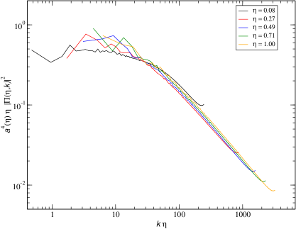
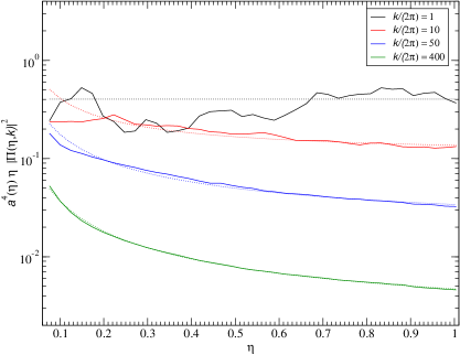
Figure 5: Rescaled equal-time correlator $a^{4}\eta|\varPi|^{2}$, in the matter era, as a function of $k\eta$ (left panel), evaluated at different conformal times $\eta$. In scaling $a^{4}\eta|\varPi|^{2}$ is stationary and the curves on the left panel tend to superimpose. The excess of power close to the Nyquist frequency is an aliasing artefact (it is removed in the final calculation). The right panel shows the same equal-time correlators but plotted as a function of $\eta$, for different wavenumbers $k$. Although the large length scale modes (small values of $k$) are in scaling at early times in the simulation, the smallest length scales are still relaxing by the end of the run. We use a fit to these relaxation curves to discard, at any given time, modes too far from scaling (see text).

In the left panel of figure 5, we have plotted this quantity as a function of $x=k\eta$ and at different times $\eta_{p}$ during the simulation. The spectrum is flat on large scales and turns to a power law decay at large $x$, with a power-law exponent slowly approaching $-1$ towards the end of the run. This shape matches the one expected for a distribution of one-dimensional objects, the change from a plateau-like shape to a power-law decay precisely occurring at the correlation length of the string network [90].

Ignoring the expected cosmic variance effects at small $x$, the different curves are quasi-superimposed one onto the others, with, however, a slowly evolving tail at large wavenumbers. Comparing the power-law tail of the anisotropic stress plotted for $\eta=0.71$ to the one at the end of the run ($\eta=1$) suggests that scaling is indeed reached up to $x\lesssim 200$. Above this value, the amplitude of the tail seems to be slightly changing with time suggesting that these small scale modes are still relaxing. This is more visible in the right panel of figure 5, in which we have plotted $a^{4}(\eta)\eta|\varPi(\eta,k)|^{2}$ as a function of $\eta$, and for different modes $k$ (solid curves). Although the large scale modes (small values of $k$) are in scaling from very early times, high wavenumbers such as $k=800\pi$ are indeed relaxing all over the simulation time.

In the same figure, the dotted curves represent, for each mode $k$, the best fit obtained by assuming the relaxation function to be a power-law decay towards a constant value. These fits allow us to determine, at any given time during the simulation, by how much a given mode of the anisotropic stress correlator differs from its expected asymptotic value. Calling the relative difference $\delta_{k}(\eta)$, we can now use it as a criterion to discard, or not, the mode when constructing the full unequal-time correlator of equation (2.22) (see next section). Clearly, discarding the values $\delta_{k}(\eta)<\delta$ with $\delta$ very small would essentially remove all modes at all times and some compromise has to be done between scaling accuracy and limiting the noise. Unless otherwise stated, we allow each mode to be, at most, from $\delta=50\%$ to the fitted and extrapolated asymptotic value. This criterion also gives the typical error we will have on the final result due to the slow convergence towards scaling of the smallest length scales.

3.4 Machine-learned correlators

From the previous discussion, we have at our disposal the correlators $\left\langle\varPi_{r}^{*}(\xi_{l},k_{q})\varPi_{r}(\xi_{p},k_{q})\right\rangle$ for some discrete values of $\xi_{l}$, $\xi_{p}$ and $k_{q}$. From equation (2.22), these numbers give us a sampling of the function $\mathcal{T}(\xi,\xi^{\prime},k)=\sum_{r}\mathcal{T}_{r}(\xi,\xi^{\prime},k)$.

3.4.1 Correlators in scaling

Figure 6: The scaling function $\mathcal{U}^{\mathrm{rad}}(\ln u,\ln v)$ reconstructed using a radial basis function decomposition based on the sparse data computed in the Nambu-Goto numerical simulations. The unequal-time correlator is maximal along the $u$ axis, i.e., at equal times. On Hubble length scales ($\ln u<0$), time correlations persist over, typically, one Hubble time. Notice the damped off-diagonal oscillations which are expected from causality. On small scales (large $\ln u$), the equal-time correlator decays as $k^{-1}$.

Figure 7: The scaling function in the matter era, $\mathcal{U}^{\mathrm{mat}}(\ln u,\ln v)$, reconstructed using a radial basis function decomposition. Notice the higher amplitude than the radiation-era function plotted in figure 6.

Let us first focus on the radiation and matter eras. The scaling ensures that $\mathcal{T}(\xi,\xi^{\prime},k)=\mathcal{U}(x,x^{\prime})$, where, as before, $x=k\eta$. One expects this function to be maximal along the diagonal $x=x^{\prime}$ as the correlations should decay at large unequal times. It is therefore convenient to work with the new variables

$$u\equiv\sqrt{xx^{\prime}}=k\sqrt{\eta\eta^{\prime}},\qquad v\equiv\sqrt{\dfrac{x^{\prime}}{x}}=\sqrt{\dfrac{\eta^{\prime}}{\eta}},$$ (3.3)

where the wavenumber dependence is now only in $u$. Moreover, since $u$ and $v$ are positive and may assume variations over a few orders of magnitude, we will be working in the $(\ln u,\ln v)$ space. In order to numerically determine the function $\mathcal{U}$ from irregular gridded data, we have used some simple machine-learning method based on a radial basis function (RBF) decomposition [96]. Basically, this consists in decomposing the function $\mathcal{U}(\ln u,\ln v)$ as a weighted sum of isotropic functions, here inverse quadratic, centered over a set of nodes in the $(\ln u,\ln v)$ space. More specifically, denoting the vector ${\boldsymbol{r}}\equiv(\ln u,\ln v)$, we fit the correlator by the function

$$\mathcal{F}({\boldsymbol{r}})=\sum_{i=1}^{N}\varpi_{i}\left[1+\dfrac{\left({\boldsymbol{r}}-{\boldsymbol{r}}_{i}\right)^{2}}{\lambda^{2}}\right]^{-1},$$ (3.4)

where $\lambda$ is a scale parameter and $N$ the total number of nodes used. The quantities ${\boldsymbol{r}}_{i}$ are the location of each node in this two-dimensional space. They have been evenly distributed along a two-dimensional grid encompassing the whole data range. The weights $\varpi_{i}$ are then computed as to minimize the difference between the $\mathcal{F}({\boldsymbol{r}}_{j})$ and $\mathcal{U}({\boldsymbol{r}}_{j})$, where the ${\boldsymbol{r}}_{j}$ are running on the actual data coming from the cosmic string simulation. For the ${\boldsymbol{r}}_{j}$, we could have used the raw sparse data, but, in order to minimize the noise, best results were obtained by binning the raw data (using a nearest neighbourg method) before feeding them to a singular value decomposition solver to invert Eq. (3.4) and determining the weights $\varpi_{i}$. Finally, the scale parameter $\lambda$ is determined by minimising the difference between the raw data (unbinned) and the radial basis function predictor. Notice that, at each fitting iteration of $\lambda$, one needs to recompute all the weights. As a matter of fact, such a decomposition is strictly equivalent to a single layer neural network having as many neurons as RBF nodes. Less than percent accuracy in the decomposition is typically achieved with a few hundred nodes ($N\gtrsim 400$).

As an illustration, figure 6 shows the resulting function $\mathcal{U}^{\mathrm{rad}}(\ln u,\ln v)$ over the range of values probed by the Nambu-Goto simulation. Most of the power is at equal times, $x=x^{\prime}$, along the $\ln v=0$ direction. A broad peak is visible on Hubble scales ($\ln u\simeq 0$) while the “crest” of the correlator starts decaying as $k^{-1}$ at large $\ln u$, the transition between the two behaviour occurring at the length scales associated with the mean inter-string distance. Non-vanishing off-diagonal values ($\ln v\neq 0$) are essentially located on Hubble scales, and, typically last for one Hubble time. Let us remark the presence of some oscillations in these regions. They are expected by causality, indeed, if correlations abruptly disappear outside the light cone in real space, then oscillations should be present in Fourier space [97]. The matter era scaling function $\mathcal{U}^{\mathrm{mat}}(\ln u,\ln v)$ has been represented in figure 7 and is of similar shape. Let us however remark the higher overall amplitude and the larger off-diagonal structures at large scales.

Let us notice that the very same correlator has been derived for Abelian Higgs string in Ref. [98] as to compute their induced CMB anisotropies. In that reference, the authors fit the off-diagonal part by a slowly decaying function, and, such a slow decay is similar to the off-diagonal behaviour we observe but on sub-Hubble scales only. However, on Hubble-scales, the presence of the off-diagonal oscillations prevented us to use this method and this is one of the reasons for having used the radial basis function method. It is nevertheless interesting to notice that Figure 8 of Ref. [98] shows some off-diagonal structures as well, on Hubble scales, which could very well be oscillatory but cut-off by the smaller dynamical range of the Abelian Higgs field simulations compared to our Nambu-Goto simulations.

Although the range of values in $u$ and $v$ accessible in the Nambu-Goto simulation covers a few orders of magnitude (see figures 6 and 7), the integrals of equation (2.25) and (2.28) are over a much larger domain. The interest of having used a RBF decomposition is that the functions $\mathcal{U}(\ln u,\ln v)$ can be evaluated outside the fitted domain. The asymptotic behaviour is there driven by the one of the radial basis functions and it decays to zero as a sum of inverse quadratic functions. However, as shown in Ref. [84], the precise asymptotic form of the equal-time correlator at large $\ln u$ (along the $\ln v=0$ direction) determines the high wavenumber shape of the final gravitational wave power spectra. As such, for the large values of $\ln u$ outside the fitting domain, we have implemented a power law extrapolation of the correlators $\mathcal{U}(\ln u,\ln v=0)\propto u^{-1}$ while keeping the RBF decomposition along the $\ln v$ direction. On the largest scales, i.e., for large negative values of $\ln u$, we have implemented a constant extrapolation as one can show that the correlator should be constant in this limit [81].

3.4.2 Transition era

As can be seen in figure 4, the energy density of long strings during the transition era slowly drifts from radiation-like values towards the one expected in a pure matter era. One should expect a similar behaviour for the anisotropic stress correlator and this motivates us to rewrite the function

$$\mathcal{T}(\eta,\eta^{\prime},k)=\mathcal{T}^{\mathrm{mix}}(\ln u,\ln v,w),$$ (3.5)

where we have introduced the new dimensionless parameter

$$w\equiv\dfrac{\eta+\eta^{\prime}}{2\bar{\eta}_{\mathrm{eq}}}.$$ (3.6)

From the previous section, one expects

$$\mathcal{T}^{\mathrm{mix}}(\ln u,\ln v,w\to 0)=\mathcal{U}^{\mathrm{rad}}(\ln u,\ln v),\qquad\mathcal{T}^{\mathrm{mix}}(\ln u,\ln v,w\gg 1)=\mathcal{U}^{\mathrm{mat}}(\ln u,\ln v),$$ (3.7)

such that $w$ encodes the relaxation time from the radiation-era correlator to the matter-era one. In practice, the matching to radiation- and matter-era is made at a finite value of $w$, one which is accessible within the transition-era simulation, here at $w=0.8$ and $w=8$.

Numerically, the sparse data extracted from the transition-era simulation have been again fitted with a RBF decomposition, but now, in the three dimensions $(\ln u,\ln v,w)$. Convergence requires a few thousand nodes, as opposed to a few hundred for the correlators in scaling, such that the computations are slightly more demanding (see section 3.4.1). But the main problem is to determine which domains in the space $(\eta,\eta^{\prime},k)$ are not too much affected by the initial conditions. Because there is no scaling any more, one cannot use the stationarity of $a^{4}(\eta)\eta|\varPi(\eta,k)|^{2}$ as a criterion of being non-contaminated by the initial conditions. Noticing that the Nambu-Goto simulation starts with a scale factor evolution which is close to the one of the radiation era, we have chosen to take cuts in the $k$ and $\eta$ domains identical to the ones of a pure radiation era, with the same value $\delta=50\%$ (see section 3.3). As we show in the next section, the contribution of the transition era to the final result remains however subdominant.

4 Gravitational waves from long strings

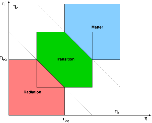
Figure 8: Conformal time domains (coloured squares) in which the anisotropic stress unequal-time correlators are determined from the radiation-era, transition-era and matter-era Nambu-Goto numerical simulations. As can be seen in figures 6 and 7, off-diagonal correlations ($\eta\neq\eta^{\prime}$) rapidly decay such that the coloured squares are covering all of the physically relevant regions. However, there are several manners to pave the three numerical simulations. Here, we have chosen to patch them at fixed value of the parameter $w=(\eta+\eta^{\prime})/(2\bar{\eta}_{\mathrm{eq}})$ (dashed lines).

4.1 Computing resources

The strain power spectrum $\mathcal{P}_{h}(\eta_{1},\eta_{2},k)$, and the energy density parameter $\Omega_{\mathrm{gw}}(\eta_{1},\eta_{2},k)$, evaluated at some possibly unequal-times, $\eta_{1}$ and $\eta_{2}$, require the computation of the kernels $K_{\mathrm{s}}(x_{i},x)$, $K_{\mathrm{e}}(x_{i},x)$ and of the function $\mathcal{T}(x/k,x^{\prime}/k,k)$ at all past times $\eta_{\mathrm{ini}}\leq\eta\leq\eta_{1,2}$. These quantities indeed appear in the three integrals $I_{\mu}$, $I_{\mu^{\prime}}$ and $I_{\kappa}$ given in equations (2.25) and (2.28). They are two-dimensional integrals over the domain $[x_{\mathrm{ini}},x_{1}]\times[x_{\mathrm{ini}},x_{2}]$ that need to be evaluated for each values of the wavenumber $k$. Figure 8 sketches the integration domain and its covering by the Nambu-Goto numerical simulations. In practice, we have fixed the value of $x_{\mathrm{ini}}=k\eta_{\mathrm{ini}}$ by assuming that the string network has been formed in the early Universe at a redshift $z_{\mathrm{ini}}=10^{30}$, which corresponds to $\eta_{\mathrm{ini}}\simeq 10^{-28}/\mathcal{H}_{0}$. As shown in section 2.2, for the exact $\Lambda$CDM model, the scale factor $a(x/k)$ appearing in the integrand can only be obtained by numerically integrating the Friedmann-Lemaître equations. The convolution kernels, evaluated at a given $(x_{i},x)$, require two additional numerical integrations of the differential operator (2.7). As such, computing these integrals is numerically demanding. For this purpose, we have used the CUBA library [99], which is a Monte-Carlo type integrator, i.e., points in the space $(x,x^{\prime})$ are randomly picked to evaluate the integrals. For each mode $k$, a target accuracy of $10^{-3}$ may typically demand drawing $5\times 10^{9}$ points, especially for large values of $k$ where the integrand fastly oscillates and this requires as much numerical integration of the scale factor and of the convolution kernels.

In order to speed-up the calculations, we have parallelised the code using the Message Passing Interface (MPI) to allow for the computation of each wavenumber $k$ to be performed on a different machine. Moreover, we have used another level of parallelism using the OpenMP directives to distribute the integrand evaluation over the different processors available on a single machine. A final speed-up of two has been reached by using the AVX2 vector registers for the most inner operation. Finally, in view of the results of section 2.2, for all wavenumbers $k\geq 10\mathcal{H}_{0}$, the calculations are simplified by neglecting the cosmological constant effects and using the analytic form (2.12) of the scale factor. This allows us to skip the numerical integration of the Friedmann-Lemaître equations, but, still, for these modes, the Green’s functions $G_{x}^{\mathrm{mix}}(x_{i})$ can only be obtained by numerically integrating equation (2.13).

4.2 Results

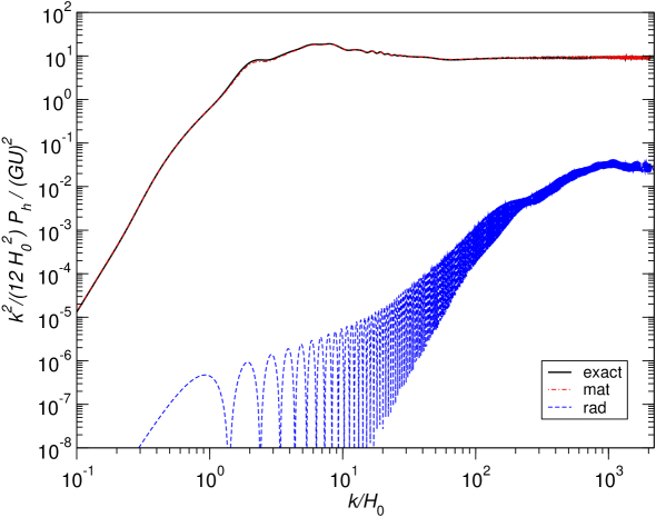
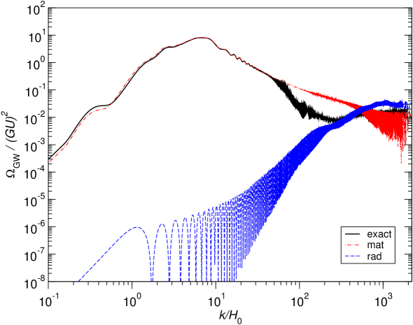
Figure 9: The GW rescaled strain power spectrum $k^{2}/(12\mathcal{H}_{0}^{2})\mathcal{P}_{h}(\eta_{0},\eta_{0},k)$ (top panel) and the energy density parameter $\Omega_{\mathrm{gw}}(\eta_{0},\eta_{0},k)$ (bottom panel), today, generated by long cosmic strings. In both panels, the black solid curve is the exact numerical result using the $\Lambda$CDM scale factor evolution and $\Lambda$CDM Green’s function for the tensor modes. The dashed curves show some semi-analytical approximations of the matter era (red) and radiation era (blue) contributions assuming an instantaneous transition between the radiation and matter era (see Ref [84] for more details on the approximation). For these, the Green’s function are analytical and given by equations (2.9) and (2.10). As expected, these approximations are very good on sub-Hubble scales and far from the wavenumbers associated with the equality radiation-matter $k_{\mathrm{eq}}/\mathcal{H}_{0}=\mathcal{O}\!\left(10^{2}\right)$.

The main results of this work are the strain power spectrum and the energy density parameter of gravitational waves, evaluated today, as a function of the wavenumber $k$. Both spectra are represented in figure 9 as black curves and have been obtained after $30000$ hours of CPU time (on AMD EPYC 7742 processors). Notice that we have plotted the rescaled strain spectrum $k^{2}/(12\mathcal{H}_{0}^{2})\mathcal{P}_{h}(\eta_{0},\eta_{0},k)$, which is the quantity of interest for local measurement of GW (see section 4.3). As discussed at length in Ref. [84], this quantity is often confused with the energy density parameter $\Omega_{\mathrm{gw}}(\eta_{0},\eta_{0},k)$ whereas both may differ (see section 2.3).

The maximal amplitude of the spectra today occurs around the Hubble scales. The maximal amplitude of the strain, and of the rescaled strain, as well as the corresponding wavenumbers, read

$$\max\left[\mathcal{P}_{h}(\eta_{0},\eta_{0},k)\right]\simeq 21(GU)^{2}\quad\textrm{at}\quad k\simeq 2.0\mathcal{H}_{0},$$ (4.1)

$$\max\left[\frac{k^{2}}{12\mathcal{H}_{0}^{2}}\mathcal{P}_{h}(\eta_{0},\eta_{0},k)\right]\simeq 19(GU)^{2}\quad\textrm{at}\quad k\simeq 7.9\mathcal{H}_{0}.$$

The energy density parameter peaks at similar values, namely $\max[\Omega_{\mathrm{gw}}(\eta_{0},\eta_{0},k)]\simeq 8.9(GU)^{2}$ at $k=6.7\mathcal{H}_{0}$.

In figure 9, we have also represented as dashed, and dot-dashed, curves some semi-analytical approximations derived in Ref. [84]. These ones are obtained by assuming an instantaneous transition between the radiation and matter eras such that the Green’s functions are all analytical and given by equations (2.9) and (2.10). The string correlators $\mathcal{U}^{\mathrm{rad}}$ and $\mathcal{U}^{\mathrm{mat}}$ are still the ones derived from simulations while the transition era is simply ignored. Let us notice that, as discussed in section 2.2, because the radiation era Green’s function is inaccurate during the matter era, the radiation-era contribution is actually derived by integrating up to equality, and then, freely propagating the modes in the matter era up to today. Compared to the exact solutions (black solid curves), we see that, provided the wavenumbers are sub-Hubbles, and not entering the Hubble radius close to equality, these approximations are quite good while being computationally faster. Moreover, because their sum is very close to the exact spectrum, this confirms that GW from the transition era remain a subdominant contribution to the overall spectra today. Only some deviations are visible in $\Omega_{\mathrm{gw}}$ in the range $k/\mathcal{H}_{0}\in[50,500]$ (see below).

Focusing on the top panel of figure 9, after the broad peak, let us notice the presence of a plateau at large wavenumbers, with high frequency oscillations superimposed (black curve). Such a plateau is indeed expected for all scaling defects evolving within the radiation era [82]. However, as can be seen in this plot, the plateau is mainly sourced by the long cosmic strings evolving within the matter era (red curve), the radiation era contribution being significantly smaller. This matter-era plateau is peculiar to long strings, these ones acting as singular sources of GW according to the classification of Ref. [84]. The fact that their contribution is higher than the strings evolving in the radiation era is non-trivial. For one part, it comes from the slow decay of $\mathcal{U}^{\mathrm{mat}}$ at large wavenumber, this is the reason why the matter contribution is flat at high frequencies. For another part, it comes from the higher values, taken over a wider domain, by the correlator $\mathcal{U}^{\mathrm{mat}}$ compared to $\mathcal{U}^{\mathrm{rad}}$ (see figures 6 and 7).

In the bottom panel of figure 9, we also see a plateau for the energy density parameter $\Omega_{\mathrm{gw}}(\eta_{0},\eta_{0},k)$, but this one is of amplitude a few orders of magnitude smaller than the one of the rescaled strain. Moreover, both the matter and radiation era contributions are about the same at high wavenumber. This is in accordance with the analytic calculations made for singular sources in Ref. [84] where, for a perfectly coherent correlator scaling as $\mathcal{U}^{\mathrm{mat}}\propto(xx^{\prime})^{-1/2}$, this ratio has been estimated as $(\eta_{\mathrm{eq}}/\eta_{0})^{2}$ (see figure 5 of that reference). More intuitively, these results mean that the stochastic strain generated by long strings is dominated by the strings close to us, the ones in the matter era. But when considering the energy density parameter, averaged over all space, redshifted GW emitted by the most numerous strings of the radiation era weight as much as the close ones. From our numerical results, we find the plateaus to have an amplitude given by

$$\max\left[\frac{k^{2}}{12\mathcal{H}_{0}^{2}}\mathcal{P}_{h}(\eta_{0},\eta_{0},k)\right] \simeq 9(GU)^{2}\quad \textrm{for}\quad k\gg k_{\mathrm{eq}},$$ (4.2)

$$\max[\Omega_{\mathrm{gw}}(\eta_{0},\eta_{0},k)] \simeq 0.015(GU)^{2}\quad \textrm{for}\quad k\gg k_{\mathrm{eq}},$$

where we have introduced $k_{\mathrm{eq}}\equiv 1/\bar{\eta}_{\mathrm{eq}}\simeq 40\mathcal{H}_{0}\simeq 0.009\,\mathrm{Mpc}^{-1}$. Let us notice, in the bottom panel, the visible deviation of the exact computation (black curve) with respect to both the matter era and radiation era semi-analytical calculations in the range $k\in[k_{\mathrm{eq}},10k_{\mathrm{eq}}]$. In this domain, GW from non-scaling strings in the transition era dominate. Around $k/\mathcal{H}_{0}\simeq 10^{3}$, the exact spectrum matches again the semi-analytical ones. Let us notice that none of the transition era effects are visible in the strain spectrum. Indeed, at all length scales, the strain spectrum remains dominated by the matter-era strings contribution.

Another remark concerns the amplitude of the oscillations at high frequencies which, in these plots, is only a few percent of the total amplitude. As discussed in Ref. [84], the actual amplitude of these oscillations depends on how fast the correlator decays in the $\ln v$ direction, but the simulations do not allow us to determine this very accurately at small scales. In particular, by design, our RBF decomposition smoothes the small structures and it is very well possible that the actual oscillation amplitude at large wavenumbers $k/\mathcal{H}_{0}>10^{3}$ growths. As analytically shown in Ref. [84], for the perfectly coherent correlator $\mathcal{U}^{\mathrm{mat}}\propto(xx^{\prime})^{-1/2}$, the oscillation amplitude would be maximal.

In summary, using the terminology of Ref. [84], the spectra plotted in figure 9 behave as “constant sources” on super-Hubble scales (i.e., grows as $k^{3}$), then, for modes of wavelength around a tenth of the Hubble radius, they transit into a broad peak driven by the shape of the unequal time correlator. These length scales are typical of the mean inter-string distance in the network, and, in this region, oscillations are washed-out by the non-vanishing off-diagonal parts of $\mathcal{U}(x,x^{\prime})$. Then, around $k_{\mathrm{eq}}$, there is a regime associated with non-scaling defects, apparent only in $\Omega_{\mathrm{gw}}$. Finally, at large wavenumbers, i.e., small length scales, the correlator becomes sharp and an oscillatory pattern around a plateau appears again (“singular” sources).

4.3 Discussion

From the observational side, the GW spectra generated by long cosmic strings are of small amplitude and only the oscillatory plateau is of relevance for today measurements made with pulsar timing arrays and laser interferometers ($H_{0}\simeq 2.2\times 10^{-18}\,\mathrm{Hz}$). From Ref. [32], the reported two-sigma upper limit $\Omega(f=50\,\mathrm{Hz})<5.8\times 10^{-9}$ can be converted, for long strings, into the upper bound $GU<2.5\times 10^{-5}$. In the nanohertz range, using the strain amplitude reported in Ref. [35], we find $k^{2}/(12\mathcal{H}_{0}^{2})\mathcal{P}_{h}(k)\lesssim 2.0\times 10^{-8}$ and $GU<4.7\times 10^{-5}$. These figures are not yet competitive with the CMB measurements [52, 55], which give $GU<\mathcal{O}\!\left(10^{-7}\right)$. However, let us stress again that these GW bounds apply to long strings that would exist only in the matter era, and these ones are essentially unconstrained by CMB physics [62]. For the future GW observatories, using the forecast $\Omega(f=10^{-3}\,\mathrm{Hz})\simeq 8\times 10^{-13}$ derived for the LISA satellites in Ref. [100], one would get down to a slightly better limit than CMB, namely $GU=10^{-7}$.

Let us clarify that, in spite of the notation, the above quantity referred to as $\Omega(f)$ is not spatially averaged and does not measure the cosmological energy density of GW. Rather, it is a rescaling of the spectral density $S_{h}(f)$ and a measure of the local strain power: $\Omega(f)=4\pi^{2}f^{3}/(3H_{0}^{2})S_{h}(f)$. It can therefore be very different than our $\Omega_{\mathrm{gw}}(\eta_{0},\eta_{0},k)$. Defining the angular frequency $\omega=2\pi f$, from equation (2.16) and (2.17), one has the correspondence

$$\mathcal{P}_{h}\left(\dfrac{k}{a_{0}}=\omega\right)\sim\dfrac{2\omega}{\pi}S_{h}(\omega),$$ (4.3)

which implies that

$$\Omega\left(f=\dfrac{\omega}{2\pi}\right)\sim\dfrac{k^{2}}{12\mathcal{H}_{0}^{2}}\mathcal{P}_{h}(k).$$ (4.4)

In these expressions, the symbol “$\sim$” signals that we blindly trade $k/a_{0}$ for $\omega$, which is an assumption. As shown in Ref. [84], any given wavenumber $k/a_{0}$ actually sources four angular frequencies $\omega=\pm k/a_{0}$ and $\omega=\pm 2k/a_{0}$. The numbers quoted above assume that these angular frequencies are all of similar amplitude.

5 Conclusion

Using Nambu-Goto numerical simulations of cosmic strings evolving in a Friedmann-Lemaître universe, we have derived the expected stochastic gravitational wave background (SGWB), today, generated by the long strings all over the cosmic history. Our main results are the strain and energy density power spectra represented in figure 9. Although of relatively small amplitude, typically $(k^{2}/\mathcal{H}_{0}^{2})\mathcal{P}_{h}\simeq 100(GU)^{2}$, this signature constitutes an absolute lower limit for most cosmic string models. Moreover, we have found that, at high wavenumbers, the gravitational waves emitted by strings in the matter era contribute more to the SGWB than the ones coming from the radiation era. This is particularly relevant for models in which strings would be reaching scaling only within the matter era [59, 61].

For deriving our result, we have solved and propagated gravitational waves of cosmological origin using a Green’s function approach. Such a method allows us to keep track of the time-dependence of gravitational waves, at all times, and that is why we are able to compute the fine oscillatory patterns in the strain and energy density power spectra. The accuracy of the method has been discussed in section 2.2, in which we have shown that using the radiation era Green’s function is incorrect as soon as an observable mode spends some time in the super-Hubble regime. On the contrary, the matter era Green’s function, given by equation (2.10), has been shown to be an acceptable approximation to the $\Lambda$CDM one at all times. Let us also notice that the treatment of the transition era is not specific to cosmic strings. As can be seen in equation (2.25), the only input needed is the correlation function $\mathcal{T}(x/k,x^{\prime}/k,k)$ associated with the anisotropic stress tensor. As such, the Green’s function method presented in this work is readily applicable to any cosmological sources of gravitational waves.

Finally, this work could be extended to the $n$-point functions of the gravitational waves, and, in particular, to the bispectrum. Cosmic strings are genuinely non-Gaussian sources of cosmological perturbations [101, 102] and it could be interesting to explore the tensor side of it. The Green’s function method is well suited for this problem as the determination of the bispectrum would involve a triple integral version of equation (2.25). Such a higher-dimensional problem would certainly require to tune our radial basis functions to be separable, in a way which has already been explored for the search of non-Gaussianities elsewhere [103, 104, 105, 106].

References

- [1] P. Auclair et al., Probing the gravitational wave background from cosmic strings with LISA, JCAP 04 (2020) 034 [1909.00819].
- [2] Y. Gouttenoire, G. Servant and P. Simakachorn, Beyond the Standard Models with Cosmic Strings, JCAP 07 (2020) 032 [1912.02569].
- [3] N. Yonemaru et al., Searching for gravitational wave bursts from cosmic string cusps with the Parkes Pulsar Timing Array, Mon. Not. Roy. Astron. Soc. 501 (2021) 701 [2011.13490].
- [4] M. Jain and A. Vilenkin, Clustering of cosmic string loops, JCAP 09 (2020) 043 [2006.15358].
- [5] H. Xing, Y. Levin, A. Gruzinov and A. Vilenkin, Spinning black holes as cosmic string factories, Phys. Rev. D 103 (2021) 083019 [2011.00654].
- [6] J.C. Aurrekoetxea, T. Helfer and E.A. Lim, Coherent Gravitational Waveforms and Memory from Cosmic String Loops, Class. Quant. Grav. 37 (2020) 204001 [2002.05177].
- [7] O.F. Hernández, The global 21-cm signal of a network of cosmic string wakes, Mon. Not. Roy. Astron. Soc. 508 (2021) 408 [2108.08220].
- [8] D.I. Dunsky, A. Ghoshal, H. Murayama, Y. Sakakihara and G. White, Gravitational Wave Gastronomy, 2111.08750.
- [9] M. Gorghetto, E. Hardy and H. Nicolaescu, Observing invisible axions with gravitational waves, JCAP 06 (2021) 034 [2101.11007].
- [10] E.J. Chun and L. Velasco-Sevilla, Tracking down the route to the SM with inflation and gravitational waves, Phys. Rev. D 106 (2022) 035008 [2112.14483].
- [11] D. Kirzhnits and A. Linde, Macroscopic consequences of the Weinberg model, Phys. Lett. B 42 (1972) 471.
- [12] I.Y. Kobsarev, L.B. Okun and Y.B. Zeldovich, Spontaneus CP-violation and cosmology, Physics Letters B 50 (1974) 340.
- [13] T.W.B. Kibble, Topology of cosmic domains and strings., J. Phys. A 9 (1976) 1387.
- [14] E. Witten, Cosmic Superstrings, Phys. Lett. B153 (1985) 243.
- [15] J. Polchinski, Cosmic superstrings revisited, AIP Conf. Proc. 743 (2004) 331 [hep-th/0410082].
- [16] M. Sakellariadou, Cosmic Strings and Cosmic Superstrings, Nucl. Phys. Proc. Suppl. 192-193 (2009) 68 [0902.0569].
- [17] E.J. Copeland and T.W.B. Kibble, Cosmic Strings and Superstrings, Proc. Roy. Soc. Lond. A466 (2010) 623 [0911.1345].
- [18] J.R. Gott III, Gravitational lensing effects of vacuum strings - Exact solutions, Astrophys. J. 288 (1985) 422.
- [19] N. Kaiser and A. Stebbins, Microwave anisotropy due to cosmic strings, Nature 310 (1984) 391.
- [20] T. Vachaspati and A. Vilenkin, Gravitational Radiation from Cosmic Strings, Phys. Rev. D31 (1985) 3052.
- [21] C.J. Hogan and M.J. Rees, Gravitational interactions of cosmic strings, Nature 311 (1984) 109.
- [22] F.R. Bouchet, D.P. Bennett and A. Stebbins, Patterns of the cosmic microwave background from evolving string networks, Nature (London) 335 (1988) 410.
- [23] F.S. Accetta and L.M. Krauss, The stochastic gravitational wave spectrum resulting from cosmic string evolution, Nucl. Phys. B319 (1989) 747.
- [24] D.P. Bennett and F.R. Bouchet, Constraints on the gravity wave background generated by cosmic strings, Phys. Rev. D43 (1991) 2733.
- [25] B. Allen and E.P.S. Shellard, Gravitational radiation from cosmic strings, Phys. Rev. D 45 (1992) 1898.
- [26] M.B. Hindmarsh and T.W.B. Kibble, Cosmic strings, Rept. Prog. Phys. 58 (1995) 477 [hep-ph/9411342].
- [27] T. Damour and A. Vilenkin, Gravitational wave bursts from cosmic strings, Phys. Rev. Lett. 85 (2000) 3761 [gr-qc/0004075].
- [28] R. Durrer, M. Kunz and A. Melchiorri, Cosmic structure formation with topological defects, Phys. Rept. 364 (2002) 1 [astro-ph/0110348].
- [29] A.A. Fraisse, C. Ringeval, D.N. Spergel and F.R. Bouchet, Small-Angle CMB Temperature Anisotropies Induced by Cosmic Strings, Phys. Rev. D78 (2008) 043535 [0708.1162].
- [30] C. Ringeval, Cosmic strings and their induced non-Gaussianities in the cosmic microwave background, Adv. Astron. 2010 (2010) 380507 [1005.4842].
- [31] T. Vachaspati, L. Pogosian and D. Steer, Cosmic Strings, Scholarpedia 10 (2015) 31682 [1506.04039].
- [32] KAGRA, Virgo, LIGO Scientific collaboration, Upper limits on the isotropic gravitational-wave background from Advanced LIGO and Advanced Virgo’s third observing run, Phys. Rev. D 104 (2021) 022004 [2101.12130].
- [33] LIGO Scientific Collaboration, Virgo Collaboration, and KAGRA Collaboration collaboration, Constraints on cosmic strings using data from the third advanced ligo–virgo observing run, Phys. Rev. Lett. 126 (2021) 241102.
- [34] NANOGrav collaboration, The NANOGrav 12.5 yr Data Set: Search for an Isotropic Stochastic Gravitational-wave Background, Astrophys. J. Lett. 905 (2020) L34 [2009.04496].
- [35] J. Antoniadis et al., The International Pulsar Timing Array second data release: Search for an isotropic gravitational wave background, Mon. Not. Roy. Astron. Soc. 510 (2022) 4873 [2201.03980].
- [36] C. Ringeval, M. Sakellariadou and F. Bouchet, Cosmological evolution of cosmic string loops, JCAP 0702 (2007) 023 [astro-ph/0511646].
- [37] J. Polchinski and J.V. Rocha, Analytic study of small scale structure on cosmic strings, Phys. Rev. D74 (2006) 083504 [hep-ph/0606205].
- [38] J.V. Rocha, Scaling solution for small cosmic string loops, Phys. Rev. Lett. 100 (2008) 071601 [0709.3284].
- [39] L. Lorenz, C. Ringeval and M. Sakellariadou, Cosmic string loop distribution on all length scales and at any redshift, JCAP 1010 (2010) 003 [1006.0931].
- [40] C. Ringeval and T. Suyama, Stochastic gravitational waves from cosmic string loops in scaling, JCAP 1712 (2017) 027 [1709.03845].
- [41] P. Binetruy, A. Bohe, T. Hertog and D.A. Steer, Gravitational wave signatures from kink proliferation on cosmic (super-) strings, Phys. Rev. D82 (2010) 126007 [1009.2484].
- [42] J.M. Wachter and K.D. Olum, Gravitational smoothing of kinks on cosmic string loops, Phys. Rev. Lett. 118 (2017) 051301 [1609.01153].
- [43] J.M. Wachter and K.D. Olum, Gravitational backreaction on piecewise linear cosmic string loops, Phys. Rev. D95 (2017) 023519 [1609.01685].
- [44] D.F. Chernoff, E.E. Flanagan and B. Wardell, Gravitational backreaction on a cosmic string: Formalism, Phys. Rev. D 99 (2019) 084036 [1808.08631].
- [45] V. Vanchurin, K.D. Olum and A. Vilenkin, Scaling of cosmic string loops, Phys. Rev. D74 (2006) 063527 [gr-qc/0511159].
- [46] J.J. Blanco-Pillado, K.D. Olum and B. Shlaer, The number of cosmic string loops, Phys.Rev. D89 (2014) 023512 [1309.6637].
- [47] J.J. Blanco-Pillado and K.D. Olum, Direct determination of cosmic string loop density from simulations, Phys. Rev. D 101 (2020) 103018 [1912.10017].
- [48] P. Auclair, C. Ringeval, M. Sakellariadou and D. Steer, Cosmic string loop production functions, JCAP 06 (2019) 015 [1903.06685].
- [49] P.G. Auclair, Impact of the small-scale structure on the Stochastic Background of Gravitational Waves from cosmic strings, JCAP 11 (2020) 050 [2009.00334].
- [50] M. Hindmarsh, S. Stuckey and N. Bevis, Abelian Higgs Cosmic Strings: Small Scale Structure and Loops, Phys. Rev. D79 (2009) 123504 [0812.1929].
- [51] M. Hindmarsh, J. Lizarraga, A. Urio and J. Urrestilla, Loop decay in Abelian-Higgs string networks, Phys. Rev. D 104 (2021) 043519 [2103.16248].
- [52] Planck collaboration, Planck 2013 results. XXV. Searches for cosmic strings and other topological defects, Astron. Astrophys. 571 (2014) A25 [1303.5085].
- [53] J. Urrestilla, N. Bevis, M. Hindmarsh and M. Kunz, Cosmic string parameter constraints and model analysis using small scale Cosmic Microwave Background data, JCAP 1112 (2011) 021 [1108.2730].
- [54] C. Ringeval and F.R. Bouchet, All Sky CMB Map from Cosmic Strings Integrated Sachs-Wolfe Effect, Phys.Rev. D86 (2012) 023513 [1204.5041].
- [55] A. Lazanu and P. Shellard, Constraints on the Nambu-Goto cosmic string contribution to the CMB power spectrum in light of new temperature and polarisation data, JCAP 1502 (2015) 024 [1410.5046].
- [56] J.D. McEwen, S.M. Feeney, H.V. Peiris, Y. Wiaux, C. Ringeval and F.R. Bouchet, Wavelet-Bayesian inference of cosmic strings embedded in the cosmic microwave background, MNRAS 472 (2017) 4081 [1611.10347].
- [57] R. Ciuca, O.F. Hernández and M. Wolman, A Convolutional Neural Network For Cosmic String Detection in CMB Temperature Maps, Mon. Not. Roy. Astron. Soc. 485 (2019) 1377 [1708.08878].
- [58] A. Vafaei Sadr, S.M.S. Movahed, M. Farhang, C. Ringeval and F.R. Bouchet, Multi-Scale Pipeline for the Search of String-Induced CMB Anisotropies, Mon. Not. Roy. Astron. Soc. 475 (2018) 1010 [1710.00173].
- [59] J. Yokoyama, Natural Way Out of the Conflict Between Cosmic Strings and Inflation, Phys.Lett. B212 (1988) 273.
- [60] E. Jeong, C. Baccigalupi and G.F. Smoot, Probing Cosmic Strings with Satellite CMB measurements, JCAP 09 (2010) 018 [1004.1046].
- [61] K. Kamada, Y. Miyamoto, D. Yamauchi and J. Yokoyama, Effects of cosmic strings with delayed scaling on CMB anisotropy, Phys.Rev. D90 (2014) 083502 [1407.2951].
- [62] C. Ringeval, D. Yamauchi, J. Yokoyama and F.R. Bouchet, Large scale CMB anomalies from thawing cosmic strings, JCAP 02 (2016) 033 [1510.01916].
- [63] G.S.F. Guedes, P.P. Avelino and L. Sousa, Signature of inflation in the stochastic gravitational wave background generated by cosmic string networks, Phys. Rev. D 98 (2018) 123505 [1809.10802].
- [64] R.-G. Cai, Z.-K. Guo and J. Liu, A New Picture of Cosmic String Evolution and Anisotropic Stochastic Gravitational-Wave Background, 2112.10131.
- [65] R. Davis and E. Shellard, COSMIC VORTONS, Nucl.Phys. B323 (1989) 209.
- [66] R.H. Brandenberger, B. Carter, A.-C. Davis and M. Trodden, Cosmic vortons and particle physics constraints, Phys. Rev. D54 (1996) 6059 [hep-ph/9605382].
- [67] Y.-F. Cai, E. Sabancilar, D.A. Steer and T. Vachaspati, Radio Broadcasts from Superconducting Strings, Phys.Rev. D86 (2012) 043521 [1205.3170].
- [68] P. Peter and C. Ringeval, A Boltzmann treatment for the vorton excess problem, JCAP 1305 (2013) 005 [1302.0953].
- [69] B. Hartmann, F. Michel and P. Peter, Excited cosmic strings with superconducting currents, Phys. Rev. D 96 (2017) 123531 [1710.00738].
- [70] M.R. Morris, J.-H. Zhao and W.M. Goss, A Nonthermal Radio Filament Connected to the Galactic Black Hole?, ApJ 850 (2017) L23 [1711.04190].
- [71] P. Auclair, P. Peter, C. Ringeval and D. Steer, Irreducible cosmic production of relic vortons, JCAP 03 (2021) 098 [2010.04620].
- [72] R.A. Battye and D.G. Viatic, Photon interactions with superconducting topological defects, Phys. Lett. B 823 (2021) 136730 [2110.13668].
- [73] P. Auclair, K. Leyde and D.A. Steer, A window for cosmic strings, 2112.11093.
- [74] B. Cyr, H. Jiao and R. Brandenberger, Massive black holes at high redshifts from superconducting cosmic strings, 2202.01799.
- [75] D.P. Bennett and F.R. Bouchet, Cosmic-string evolution, Phys. Rev. Lett. 63 (1989) 2776.
- [76] D.P. Bennett and F.R. Bouchet, High-resolution simulations of cosmic-string evolution. I. Network evolution, Phys. Rev. D 41 (1990) 2408.
- [77] B. Carter, Essentials of classical brane dynamics, Int. J. Theor. Phys. 40 (2001) 2099 [gr-qc/0012036].
- [78] U.-L. Pen, D.N. Spergel and N. Turok, Cosmic structure formation and microwave anisotropies from global field ordering, Phys. Rev. D 49 (1994) 692.
- [79] R. Durrer and Z.H. Zhou, Large scale structure formation with global topological defects: A New formalism and its implementation by numerical simulations, Phys. Rev. D 53 (1996) 5394 [astro-ph/9508016].
- [80] J. Magueijo, A. Albrecht, D. Coulson and P. Ferreira, Doppler peaks from active perturbations, Phys. Rev. Lett. 76 (1996) 2617 [astro-ph/9511042].
- [81] R. Durrer and M. Kunz, Cosmic microwave background anisotropies from scaling seeds: Generic properties of the correlation functions, Phys. Rev. D57 (1998) R3199 [astro-ph/9711133].
- [82] D.G. Figueroa, M. Hindmarsh and J. Urrestilla, Exact Scale-Invariant Background of Gravitational Waves from Cosmic Defects, Phys. Rev. Lett. 110 (2013) 101302 [1212.5458].
- [83] D.G. Figueroa, M. Hindmarsh, J. Lizarraga and J. Urrestilla, Irreducible background of gravitational waves from a cosmic defect network: update and comparison of numerical techniques, Phys. Rev. D 102 (2020) 103516 [2007.03337].
- [84] D.C.N. da Cunha and C. Ringeval, Interferences in the Stochastic Gravitational Wave Background, JCAP 08 (2021) 005 [2104.14231].
- [85] V.F. Mukhanov, H.A. Feldman and R.H. Brandenberger, Theory of cosmological perturbations. part 1. classical perturbations. part 2. quantum theory of perturbations. part 3. extensions, Phys. Rept. 215 (1992) 203.
- [86] M. Zaldarriaga and U. Seljak, An all sky analysis of polarization in the microwave background, Phys. Rev. D 55 (1997) 1830 [astro-ph/9609170].
- [87] S. Alexander and J. Martin, Birefringent gravitational waves and the consistency check of inflation, Phys. Rev. D 71 (2005) 063526 [hep-th/0410230].
- [88] C. Caprini and D.G. Figueroa, Cosmological Backgrounds of Gravitational Waves, Class. Quant. Grav. 35 (2018) 163001 [1801.04268].
- [89] Planck collaboration, Planck 2018 results. VI. Cosmological parameters, Astron. Astrophys. 641 (2020) A6 [1807.06209].
- [90] J.H.P. Wu, P.P. Avelino, E.P.S. Shellard and B. Allen, Cosmic strings, loops, and linear growth of matter perturbations, Int. J. Mod. Phys. D 11 (2002) 61 [astro-ph/9812156].
- [91] N. Bevis, M. Hindmarsh, M. Kunz and J. Urrestilla, Cmb power spectrum contribution from cosmic strings using field-evolution simulations of the abelian higgs model, Phys. Rev. D75 (2007) 065015 [astro-ph/0605018].
- [92] A. Lazanu, E. Shellard and M. Landriau, CMB power spectrum of Nambu-Goto cosmic strings, Phys. Rev. D91 (2015) 083519 [1410.4860].
- [93] T. Vachaspati and A. Vilenkin, Formation and evolution of cosmic strings, Phys. Rev. D30 (1984) 2036.
- [94] E. Sefusatti, M. Crocce, R. Scoccimarro and H. Couchman, Accurate Estimators of Correlation Functions in Fourier Space, Mon. Not. Roy. Astron. Soc. 460 (2016) 3624 [1512.07295].
- [95] M. Frigo and S.G. Johnson, The design and implementation of FFTW3, Proceedings of the IEEE 93 (2005) 216.
- [96] D. Broomhead and D. Lowe, Multivariable functional interpolation and adaptive networks, Complex Systems 2 (1988) 321.
- [97] N. Turok, Causality and the Doppler Peaks, Phys. Rev. D54 (1996) 3686 [astro-ph/9604172].
- [98] D. Daverio, M. Hindmarsh, M. Kunz, J. Lizarraga and J. Urrestilla, Energy-momentum correlations for Abelian Higgs cosmic strings, Phys. Rev. D 93 (2016) 085014 [1510.05006].
- [99] T. Hahn, CUBA: A Library for multidimensional numerical integration, Comput. Phys. Commun. 168 (2005) 78 [hep-ph/0404043].
- [100] G. Boileau, A. Lamberts, N. Christensen, N.J. Cornish and R. Meyer, Spectral separation of the stochastic gravitational-wave background for LISA in the context of a modulated Galactic foreground, Mon. Not. Roy. Astron. Soc. 508 (2021) 803 [2105.04283].
- [101] M. Hindmarsh, C. Ringeval and T. Suyama, The CMB temperature bispectrum induced by cosmic strings, Phys. Rev. D80 (2009) 083501 [0908.0432].
- [102] M. Hindmarsh, C. Ringeval and T. Suyama, The CMB temperature trispectrum of cosmic strings, Phys. Rev. D81 (2010) 063505 [0911.1241].
- [103] J.R. Fergusson, M. Liguori and E.P.S. Shellard, General CMB and Primordial Bispectrum Estimation I: Mode Expansion, Map-Making and Measures of f_NL, Phys. Rev. D 82 (2010) 023502 [0912.5516].
- [104] J.R. Fergusson, M. Liguori and E.P.S. Shellard, The CMB Bispectrum, JCAP 12 (2012) 032 [1006.1642].
- [105] D. Regan and M. Hindmarsh, The bispectrum of cosmic string temperature fluctuations including recombination effects, JCAP 10 (2015) 030 [1508.02231].
- [106] M. Shiraishi, M. Liguori, J.R. Fergusson and E.P.S. Shellard, General modal estimation for cross-bispectra, JCAP 06 (2019) 046 [1904.02599].