Joint diagnostic test of regression discontinuity designs: multiple testing problem

Abstract

Current diagnostic tests for regression discontinuity (RD) design face a multiple testing problem. We find a massive over-rejection of the identifying restriction among empirical RD studies published in top-five economics journals. Each test achieves a nominal size of $5\%$; however, the median number of tests per study is $12$. Consequently, more than one-third of studies reject at least one of these tests and their diagnostic procedures are invalid for justifying the identifying assumption. We offer a joint testing procedure to resolve the multiple testing problem. Our procedure is based on a new joint asymptotic normality of local linear estimates and local polynomial density estimates. In simulation studies, our joint testing procedures outperform the Bonferroni correction. We implement the procedure as an R package, rdtest, with two empirical examples in its vignettes.

1 Introduction

Diagnostic tests are vital to regression discontinuity (RD) designs. The typical procedure is to evaluate the testable restrictions implied by a single non-testable identifying restriction, local randomization (Lee, 2008). However, these tests are often run separately without appropriate size control. Consequently, current procedures face multiple testing problems.

We document the severity of the multiple testing problem in a meta-analysis of recently published $60$ empirical RD studies in economics top-five journals. We find a severe size distortion in diagnostic tests. On average, each study runs $14$ tests separately for testable restrictions induced by the single identifying restriction. Each test achieves its nominal size of $5\%$; consequently, at least one testable restriction is rejected in $35\%$ of the studies. Hence, the current diagnostic procedure is useless for evaluating the validity of identification.

In this study, we resolve the multiple testing problem by offering a simultaneous testing procedure. Our procedure is based on our new theoretical results of joint asymptotic normality of nonparametric RD estimates. We consider two different test statistics: (1) a Wald (chi-squared) statistic of the sum of squared statistics and (2) a Max test statistic of the maximum squared statistics. The two test statistics complement the detection of different types of alternative hypotheses. However, we observe that the conventional Wald statistic does not attain the nominal size, possibly because of poor inverse estimation of the variance matrix. We bypass this problem by standardizing and calculating the squared sum. We demonstrate that both the standardized Wald and Max statistics exhibit superior power properties against the Bonferroni correction in numerical simulations.

We contribute to the literature on diagnostic procedures for RD designs. McCrary (2008) develops the density test, and Lee (2008) concludes that the null hypotheses of the density and balance or placebo tests are the consequences of his local randomization concept. Several theoretical studies have improved these procedures: Otsu, Xu, and Matsushita (2013) propose an empirical likelihood-based density test; Cattaneo, Jansson, and Ma (2020) consider a test based on a local polynomial estimation of the density function; Bugni and Canay (2021) propose an approximate sign test of the density test. Nevertheless, none of the aforementioned studies consider the joint procedure of these tests, and the practices of diagnostic tests follow a similar pattern: separate multiple testing of these diagnostic tests or some joint procedure without considering the nonparametric nature of the test statistics. In this study, we provide the joint testing of the consequences of a single identifying restriction in RD designs. We also provide statistical software, rdtest, that is an explicit wrapper of two standard packages, rdrobust (Calonico, Cattaneo, Farrell, and Titiunik, 2017) and rddensity (Cattaneo, Jansson, and Ma, 2018). Consequently, we provide an easy-to-implement joint diagnostic procedure based on widely used procedures.

Among these studies of diagnostic procedures, our study is particularly related to Canay and Kamat (2018) that deliver a randomization test for the balance test with a joint testing procedure. On the one hand, our procedure is based on the widely used test statistics of the density test as well as of the balance or placebo test. On the other hand, the procedure in Canay and Kamat (2018) is a randomization test for the direct implication of the local randomization (Lee, 2008). Recently, an alternative RD strategy has been proposed with a substantially stronger but explicit assumption of local randomization for a small sample study (Cattaneo, Frandsen, and Titiunik, 2015 and Cattaneo, Titiunik, and Vazquez-Bare, 2016). The randomization test of Canay and Kamat (2018) may be applied to a small sample study including the latest alternative RD strategy. Furthermore, our meta-analysis confirms the critical nature of the multiple testing problem in the RD diagnostic context. Our simulation evidence also deepens the understanding of the joint test statistics, which choice has been briefly discussed in Canay and Kamat (2018). Consequently, we complement Canay and Kamat (2018) by offering a complementary testing procedure and demonstrating the need for a joint testing procedure in RD designs.

Moreover, we contribute to the asymptotic theory of nonparametric estimates. We show the joint asymptotic normality of multiple local polynomial estimates for the conditional mean functions and a density function. Calonico, Cattaneo, and Titiunik (2014) show the asymptotic normality of a single local polynomial estimate for a conditional mean function at a boundary point after bias correction. Cattaneo, Jansson, and Ma (2020) show the asymptotic normality of a local polynomial estimate of a density function at a boundary point. As a key feature of our joint normality result, we do not impose any restrictions on the choice of bandwidths apart from the original rate conditions. Consequently, we accommodate the same mean squared error (MSE) optimal estimates for the balance and placebo test (Calonico et al., 2014) and density test (Cattaneo et al., 2020).

The rest of the paper proceeds as follows: Section 2 demonstrates the multiple testing problem in the meta-analysis, Section 3.1 shows the joint asymptotic normality of the nonparametric estimates, Section 3.2 proposes our joint tests, Section 4 demonstrates the performance of our tests in simulation, and Section 5 concludes the study by recommending practices and future research questions. Appendix A provides all the formal results and their proofs.

2 Current practices of diagnostic tests

The current diagnostic procedure includes two different tests: (1) the density test evaluates the continuity of a density function, and (2) the balance or placebo test evaluates the continuity of the conditional mean functions of pre-treatment covariates. Both testable restrictions result from the consequence of the local randomization (Lee, 2008) and local randomization implies point identification. If any of these implied restrictions are false, then the local randomization is false. However, the rejection of any particular test is uninformative; only the joint null of the testable restrictions is informative. Consequently, evaluating each test separately results in the multiple testing problem for validating local randomization.

We quantify the severity of the multiple testing problem by conducting a meta-analysis of RD studies published in the top-five economics journals. In Table 1, the summary statistics are presented for $60$ papers that satisfy our search criterion (see Appendix B for details). On average, each empirical study ran approximately $14$ tests, whereas the median study ran $12$ tests. As shown in Figure 2(a), many studies ran as many as $20$ tests, and a few studies ran more than $30$ tests.

Table 1: Summary Statistics

	mean	sd	median	min	max
Number of tests per study	14.17	9.51	12	1	45
Rejecting at least one hypothesis	0.35	0.48	0	0	1
Number of rejected tests per study	0.75	1.54	0	0	9
Number of studies	60

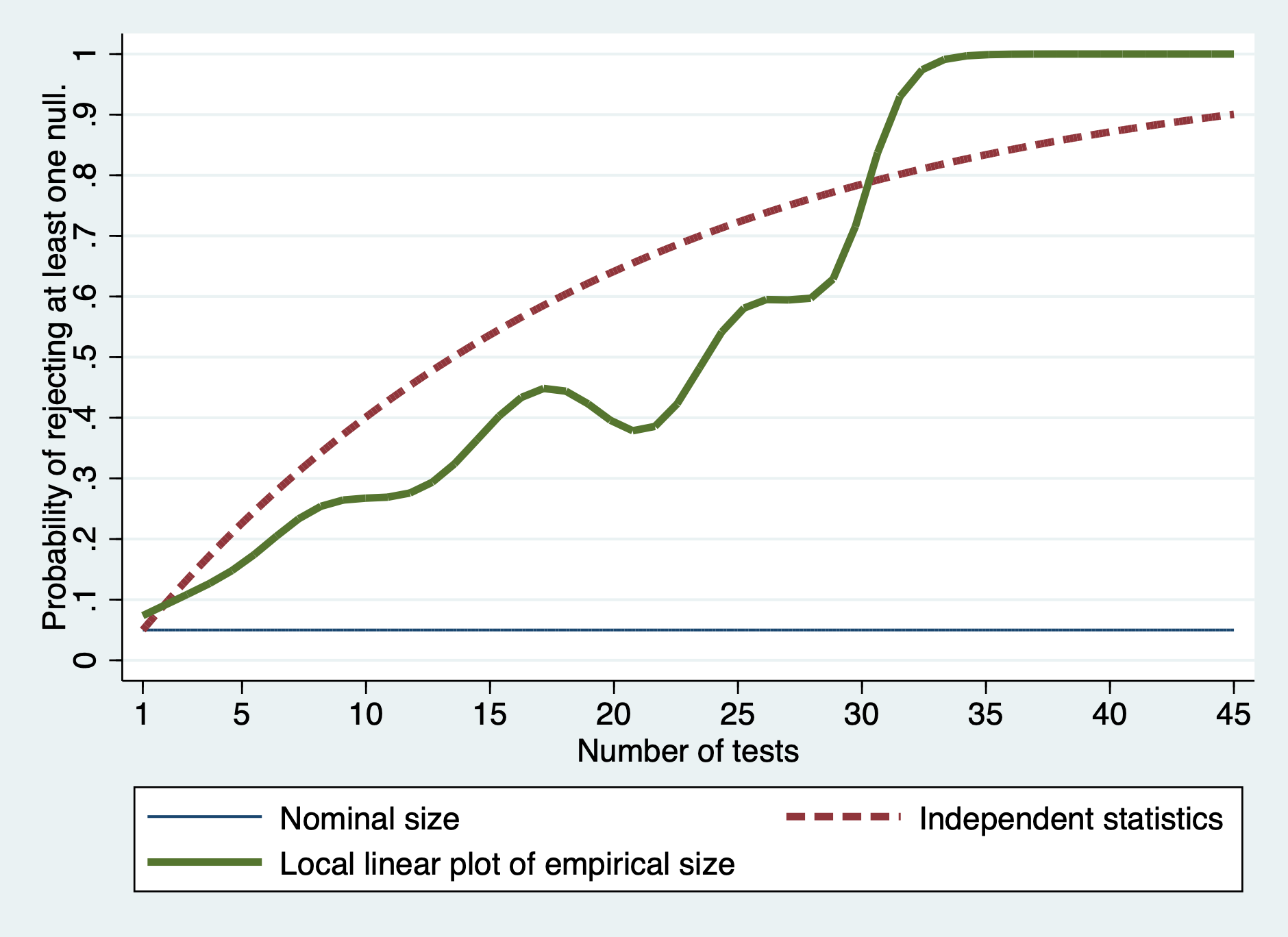
Figure 1: Theoretical and empirical rejection probability by the number of tests

Over-rejection of the joint null is evident. Table 1 presents the rejection probability of the joint null hypothesis. Among the $60$ studies, more than one-third of them reject at least one null hypothesis. Figure 1 shows the plot of rejection probabilities of the joint null over the number of tests per study. The dashed line is the theoretical rejection probabilities of the joint null hypothesis for independent test statistics, and the solid line is the local linear estimate of the empirical rejection probabilities of the joint null hypothesis using the data. The joint null hypothesis is massively over-rejected.

Two types of evidence indicate that multiple testing problem causes the massive over-rejection: first, the realized $p$-values follow a uniform distribution on $[0,1]$ as in the null hypothesis; second, the empirical rejection probability is close to $5\%$ for each balance test and density test separately. Figure 2(b) shows the quantile plot of $p$-values against the uniform distribution. Table 2 reports the empirical rejection probability for each balance test and density test separately. Among the 776 balance and 23 density tests reported with their test statistics values, their empirical rejection probabilities are $4.64$% and $4.35$%; apparently, each test is valid and must have been honestly reported as separate tests. Hence, local randomization failure is unlikely to be a cause of the over-rejection. The multiple testing problem causes the massive over-rejection of the joint null hypothesis.

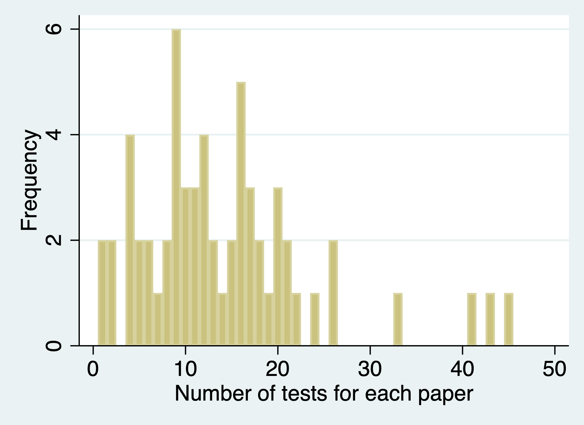
(a) Histogram of the number of tests

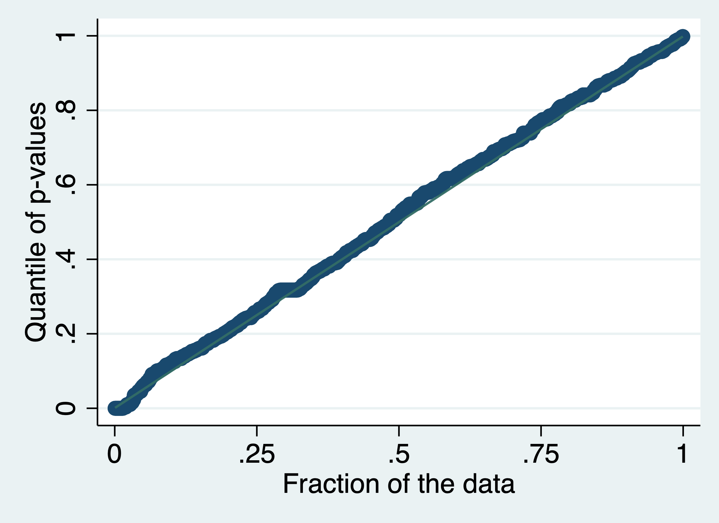
(b) Quantile plot of p-values of tests

Figure 2: Descriptive plots of papers and their tests

Table 2: Rejection probabilities by type of tests

	Balance	Density	Total
Reject	4.64	4.35	4.63
Not	95.36	95.65	95.37
Number of tests	776	23	799

Implications from our meta-analysis are stronger than usual meta-analyses to detect publication bias among studies that search for non-null effects. The test statistic distribution of the effect-finding tests cannot be distinguished in two scenarios: first, the distribution is in the null hypothesis and contaminated owing to publication bias; second, the distribution is in the alternative hypothesis and not contaminated. Within our meta-analysis, most studies exploit institutional features in which the score is likely to be locally randomized. Hence, these null hypotheses in the diagnostic tests are likely to hold. Consequently, the realized distribution, which is close to the null distribution, provides robust evidence for non-contaminated honest reports from each study.

3 Joint asymptotic normality and our testing procedure

In Section 2, we demonstrate that the multiple testing problem causes the over-rejection. We resolve the problem by presenting our joint tests in two steps. First, we present a theoretical basis for our alternative procedure for testing the joint null hypothesis. Second, we propose two test statistics for joint manipulation testing.

3.1 New joint normality result

We derive the joint asymptotic normality of the nonparametric local polynomial estimators evaluated at the boundary of the support. Let $(Z_{1,i},\ldots,Z_{d,i},X_{i})^{\prime}$, $i=1,\ldots,n$ denote the observed random samples, $X_{i}$ denote the running variable with density $f(x)$ with respect to the Lebesgue measure, and $Z_{i}=(Z_{1,i},\ldots,Z_{d,i})^{\prime}$ denote the pre-treatment covariates. Given a known threshold $\bar{x}$, which we set at $\bar{x}=0$ without loss of generality, let the running variable $X_{i}$ determine whether unit $i$ is assigned a treatment ($X_{i}\geq 0$) or not ($X_{i}<0$).

We aim to test whether the density of the running variable $f(x)$ and the conditional expectations of the pre-treatment covariates $\mu_{Z_{k}}(x)=E[Z_{k,i}|X_{i}=x]$ for $k=1,\ldots,d$ are continuous at $x=0$. Specifically, we consider the joint null and alternative hypotheses as shown below:

$$H_{0}:(\tau_{f},\tau_{Z_{1}},\ldots,\tau_{Z_{d}})=0\quad\text{vs}\quad H_{1}:(\tau_{f},\tau_{Z_{1}},\ldots,\tau_{Z_{d}})\neq 0,$$

where $\tau_{f}=f_{+}-f_{-}$, $\tau_{Z_{k}}=\mu_{Z_{k}+}-\mu_{Z_{k}-}$, $f_{+}=\lim_{x\to 0^{+}}f(x)$, $f_{-}=\lim_{x\to 0^{-}}f(x)$, $\mu_{Z_{k}+}=\lim_{x\to 0^{+}}\mu_{Z_{k}}(x)$, $\mu_{Z_{k}-}=\lim_{x\to 0^{-}}\mu_{Z_{k}}(x)$.

Following Calonico et al. (2014) and Cattaneo et al. (2020), we use local polynomial regressions to approximate the unknown functions $f(x)$ and $\mu_{Z_{k}}(x)$ for $k=1,\ldots,d$ flexibly near the cutoff $\bar{x}=0$. See, for example, Fan and Gijbels (1996) for a review of local polynomial regressions. Based on the testing problem, we need to estimate two distinct estimands for each function using the two subsamples $\{X_{i}:X_{i}\geq 0\}$ (approximation from the right) and $\{X_{i}:X_{i}<0\}$ (approximation from the left) at a boundary point $x=0$. We chose these estimators because of their excellent boundary properties.

Using a polynomial expansion, we construct smooth local one-sided approximations of the sample average of $Z_{k,i}$ and obtain the estimators $\hat{\mu}_{Z_{k}+,p}(h_{k,n})$ and $\hat{\mu}_{Z_{k}-,p}(h_{k,n})$ as the intercepts in the local polynomial regression. Specifically, we estimate $\tau_{Z_{k}}$ using the following $p$th-order local polynomial estimators: for some $p\geq 1$ and for each $k=1,\ldots,d$,

$$\hat{\tau}_{Z_{k},p}(h_{k,n})=\hat{\mu}_{Z_{k}+,p}(h_{k,n})-\hat{\mu}_{Z_{k}-,p}(h_{k,n}),$$

$$\hat{\mu}_{Z_{k}+,p}(h_{k,n}) = e_{0}^{\prime}\hat{\beta}_{Z_{k}+,p}(h_{k,n}),$$ (3.1)

$$\hat{\mu}_{Z_{k}-,p}(h_{k,n}) = e_{0}^{\prime}\hat{\beta}_{Z_{k}-,p}(h_{k,n}),$$ (3.2)

where

$$\hat{\beta}_{Z_{k}+,p}(h_{k,n}) = \operatorname*{arg\,min}_{\beta\in\mathbb{R}^{p+1}}\sum_{i=1}^{n}1\{X_{i}\geq 0\}(Z_{k,i}-r_{p}(X_{i})^{\prime}\beta)^{2}K(X_{i}/h_{k,n})/h_{k,n},$$ (3.3)

$$\hat{\beta}_{Z_{k}-,p}(h_{k,n}) = \operatorname*{arg\,min}_{\beta\in\mathbb{R}^{p+1}}\sum_{i=1}^{n}1\{X_{i}<0\}(Z_{k,i}-r_{p}(X_{i})^{\prime}\beta)^{2}K(X_{i}/h_{k,n})/h_{k,n},$$ (3.4)

$e_{0}=(1,0,\ldots,0)^{\prime}$ is the first $(p+1)$-dimensional unit vector, $r_{p}(x)=(1,x,\ldots,x^{p})^{\prime}$ is a $p$th order polynomial expansion, $K(\cdot)$ is a kernel function, and $h_{k,n}$ is a positive bandwidth sequence.

Similarly, using a polynomial expansion, we construct smooth local one-sided approximations to the empirical distribution of $X_{i}$ and obtain the estimators $\hat{f}_{+,p}(h_{f,n})$ and $\hat{f}_{-,p}(h_{f,n})$ as the slope coefficient in the local polynomial regression. Specifically, we estimate $\tau_{f}$ using the following $p$th-order local polynomial estimator: for some $p\geq 1$,

$$\hat{\tau}_{f,p}(h_{f,n})=\hat{f}_{+,p}(h_{f,n})-\hat{f}_{-,p}(h_{f,n}),$$

$$\hat{f}_{+,p}(h_{f,n}) = e_{1}^{\prime}\hat{\beta}_{f+,p}(h_{f,n}),$$ (3.5)

$$\hat{f}_{-,p}(h_{f,n}) = e_{1}^{\prime}\hat{\beta}_{f-,p}(h_{f,n}),$$ (3.6)

where

$$\hat{\beta}_{f+,p}(h_{f,n})=\operatorname*{arg\,min}_{\beta\in\mathbb{R}^{p+1}}\sum_{i=1}^{n}1\{X_{i}\geq 0\}(\tilde{F}(X_{i})-r_{p}(X_{i})^{\prime}\beta)^{2}K(X_{i}/h_{f,n})/h_{f,n},$$ (3.7)

$$\hat{\beta}_{f-,p}(h_{f,n})=\operatorname*{arg\,min}_{\beta\in\mathbb{R}^{p+1}}\sum_{i=1}^{n}1\{X_{i}<0\}(\tilde{F}(X_{i})-r_{p}(X_{i})^{\prime}\beta)^{2}K(X_{i}/h_{f,n})/h_{f,n},$$ (3.8)

$e_{1}=(0,1,0,\ldots,0)^{\prime}$ is the second $(p+1)$-dimensional unit vector; $\tilde{F}(x)\equiv n^{-1}\sum_{i=1}^{n}$
$1\{X_{i}\leq x\}$ is the empirical distribution function of $X_{i}$; $h_{f,n}$ is a positive bandwidth sequence.

We derive the asymptotic distributions of the local polynomial estimators based on the following assumptions in Calonico et al. (2014) or Cattaneo et al. (2020).

Assumption 1.

For some $\kappa_{0}>0$, the following holds on $(-\kappa_{0},0)\cup(0,\kappa_{0})$ around the cutoff $\bar{x}=0$.

1. $f(x)$ is $R$ times continuously differentiable for some $R\geq 1$ and bounded away from zero.

2. For $k=1,\ldots,d$, $\mu_{Z_{k}}(x)$ is $S$ times continuously differentiable for some $S\geq 1$, $\operatorname{Var}(Z_{k,i}|X_{i}=x)$ is continuous and bounded away from zero, and $E[|Z_{k,i}|^{4}|X_{i}=x]$ is bounded.

Assumption 1 is a set of basic regularity conditions for the data-generating process. Assumption 1 (a) ensures that the density of the running variable is well-defined and sufficiently smooth and that the observed values are arbitrarily close to the cutoff for large samples. Assumption 1 (b) ensures that the conditional expectations and variances of the pre-treatment covariates are well-defined and have sufficient smoothness with the existence of the fourth moments.

Assumption 2.

For some $\kappa>0$, the kernel function $K(\cdot):[-\kappa,\kappa]\to\mathbb{R}$ is symmetric, bounded, and nonnegative; it is zero outside the support, and positive and continuous on $(-\kappa,\kappa)$.

Assumption 2 is a set of standard conditions for the kernel function and is satisfied for kernels commonly utilized in empirical work, such as the triangular and uniform kernels. Our results can be extended to accommodate kernels with unbounded supports or asymmetric kernels with more complex notations.

In the following, let $l,p\in\mathbb{N}$; $h_{n}=(h_{1,n},\ldots,h_{d,n})^{\prime}$; $h_{max,n}=\max\{h_{1,n},\ldots,h_{d,n}\}$; $h_{min,n}=\min\{h_{1,n},\ldots,h_{d,n}\}$; we assume all limits as $n\to\infty$ (and $h_{k,n},h_{f,n}\to 0$) unless stated otherwise. Whenever there is no confusion, we drop the sample size $n$ sub-index notation.

We provide the joint asymptotic distribution for the local polynomial estimators:

Theorem 1.

Suppose Assumptions 1 and 2 hold with $R\geq p$ and $S\geq l+2$. If $nh_{min}\to\infty$, $nh_{f}^{2}\to\infty$, $n(h_{max})^{2l+3}\to 0$, and $n(h_{f})^{2p+1}\to 0$, then:

$$\begin{split}\sqrt{n}[&\sqrt{h_{1}}(\hat{\tau}_{Z_{1},l}(h_{1})-\tau_{Z_{1}}),\ldots,\sqrt{h_{d}}(\hat{\tau}_{Z_{d},l}(h_{d})-\tau_{Z_{d}}),\sqrt{h_{f}}(\hat{\tau}_{f,p}(h_{f})-\tau_{f})]^{\prime}\\ \stackrel{{\scriptstyle d}}{{\to}}&N_{d+1}(0,V_{l,p}),\end{split}$$

where $N_{d+1}(\mu,\Sigma)$ denotes the multivariate normal distribution with $(d+1)$-dimensional mean vector $\mu$ and $(d+1)\times(d+1)$ covariance matrix $\Sigma$, and

$$V_{l,p}=\begin{pmatrix}V_{Z,l}&0\\ 0&V_{f,p}\end{pmatrix}.$$

The exact forms of $V_{Z,l}$ and $V_{f,p}$ are provided in Appendix A.3.

In Theorem 1, we show that the joint asymptotic distribution of $\hat{\tau}_{f,p}(h_{f})$ and $\hat{\tau}_{Z_{k},l}(h_{k})$ is a multivariate normal distribution under the same set of conditions as in Calonico et al. (2014) for $\hat{\tau}_{Z_{k},l}(h_{k})$ and Cattaneo et al. (2020) for $\hat{\tau}_{f,p}(h_{f})$. Hence, our joint distributional approximation is a natural generalization of the distributional approximation of each local polynomial estimator.

Remark 1 (Bandwidth Selection).

If the conditions stated in Theorem 1 are satisfied, we allow the bandwidths to be different. Hence, we may apply the MSE-optimal bandwidths derived in Calonico et al. (2014) for $h_{1},\ldots,h_{d}$ and Cattaneo et al. (2020) for $h_{f}$ to our joint distributional approximation.

Remark 2 (Asymptotic Covariance Matrix).

As in Theorem 1, the covariance matrix of $(\hat{\tau}_{Z_{1},l}(h_{1}),\ldots,\hat{\tau}_{Z_{d},l}(h_{d}))^{\prime}$ and variance of $\hat{\tau}_{f,p}(h_{f})$ are asymptotically orthogonal. Orthogonality simplifies the estimation of the overall asymptotic covariance matrix because the asymptotic covariance of $\hat{\tau}_{f,p}(h_{f})$ and $\hat{\tau}_{Z_{k},l}(h_{k})$ is known to be 0.

We propose an estimator of the asymptotic covariance matrix as follows:

$$\hat{V}_{l,p}(h)=\begin{pmatrix}\hat{V}_{Z,l}(h)&0\\ 0&\hat{V}_{f,p}(h_{f})\end{pmatrix},$$

where

$$\hat{V}_{Z,l}(h)\stackrel{{\scriptstyle P}}{{\to}}V_{Z,l},\quad\hat{V}_{f,p}(h_{f})\stackrel{{\scriptstyle P}}{{\to}}V_{f,p}.$$

We may use the estimators proposed by Calonico et al. (2014) and Cattaneo et al. (2020) for the asymptotic variances of $\hat{\tau}_{Z_{k},l}(h_{k})$ and $\hat{\tau}_{f,p}(h_{f})$ for each diagonal element of the asymptotic covariance matrix $\hat{V}_{Z,l}(h)$ and $\hat{V}_{f,p}(h_{f})$. For the covariance estimators of $\hat{\tau}_{Z_{j},l}(h_{j})$ and $\hat{\tau}_{Z_{k},l}(h_{k})$, we follow Calonico et al. (2014): an estimator of the elements of $\hat{V}_{Z,l}(h)$ based on the nearest-neighbor estimation, which may be more robust than plugging in the corresponding residuals of the nonparametric regressions in finite samples. We provide the exact forms of $\hat{V}_{Z,l}(h)$ and $\hat{V}_{f,p}(h_{f})$ in Appendix A.3.

3.2 Proposed joint tests

Given the joint asymptotic normality result, we introduce two test statistics for the joint manipulation test: (1) using the $L^{2}$-norm and (2) using the $L^{\infty}$-norm.

The Wald (chi-squared) test statistic with the $L^{2}$-norm is in the following form.

$$\hat{\chi}^{2}_{0,l,p}(h)=||(\hat{V}_{l,p}(h))^{-1/2}\hat{T}_{0,l,p}(h)||^{2}_{2},$$

where

$$\hat{T}_{0,l,p}(h)=\sqrt{n}[\sqrt{h_{1}}\hat{\tau}_{Z_{1},l}(h_{1}),\ldots,\sqrt{h_{d}}\hat{\tau}_{Z_{d},l}(h_{d}),\sqrt{h_{f}}\hat{\tau}_{f,p}(h_{f})]^{\prime}.$$

This conventional test statistic suffers from severe size distortions in the finite samples. In particular, for a sufficiently large dimension $d$, the inverse of the asymptotic covariance matrix estimator becomes unstable.

Instead, we propose the “standardized Wald (sWald) test” statistic, which modifies the form of the Wald test statistic. Particularly, we standardize the diagonal elements only and do not multiply the entire matrix by the inverse of the asymptotic covariance matrix. Our “sWald” test statistic is in the following form:

$$\tilde{\chi}^{2}_{0,l,p}(h)=||\tilde{T}_{0,l,p}(h)||^{2}_{2},$$

where

$$\tilde{T}_{0,l,p}(h)=\operatorname{diag}\{(\hat{V}_{Z_{1},l}(h))^{-1/2},\ldots,(\hat{V}_{Z_{d},l}(h))^{-1/2},(\hat{V}_{f,p}(h_{f}))^{-1/2}\}\hat{T}_{0,l,p}(h),$$

and $\operatorname{diag}(a_{1},\ldots,a_{n})$ is the $(n\times n)$ diagonal matrix with diagonal elements $a_{1},\ldots,a_{n}$.

The asymptotic distribution of $\tilde{\chi}^{2}_{0,l,p}(h)$ is obtained from the joint asymptotic distribution for the local polynomial estimators, with their diagonal elements standardized by their standard errors $(\hat{V}_{f,p}(h_{f}))^{-1/2}$ and $(\hat{V}_{Z_{k},l}(h))^{1/2}$. The standard errors of $\tau_{Z_{k}}$ are constructed as $\hat{V}_{Z_{k},l}(h)\stackrel{{\scriptstyle P}}{{\to}}V_{Z_{k},l}$, where $V_{Z_{k},l}$ is the asymptotic variance of $\sqrt{n}\sqrt{h_{k}}(\hat{\tau}_{Z_{k},l}(h_{k})-\tau_{Z_{k}})$. The asymptotic covariance matrix of the standardized local polynomial estimators is the asymptotic correlation matrix of the local polynomial estimators of $\tau_{f}$ and $\tau_{Z_{k}}$. The correlation matrix $V^{*}_{l,p}$ is

$$V^{*}_{l,p}=\begin{pmatrix}V^{*}_{Z,l}&0\\ 0&1\end{pmatrix},$$

where $V^{*}_{Z,l}=\operatorname{diag}(V_{Z_{1},l}^{-1/2},\ldots,V_{Z_{d},l}^{-1/2})V_{Z,l}\operatorname{diag}(V_{Z_{1},l}^{-1/2},\ldots,V_{Z_{d},l}^{-1/2})$; our estimator of $V^{*}_{l,p}$ is

$$\hat{V}^{*}_{l,p}(h)=\begin{pmatrix}\hat{V}^{*}_{Z,l}(h)&0\\ 0&1\end{pmatrix},$$

where

$$\hat{V}^{*}_{Z,l}(h)=D_{\hat{V}}(h)\hat{V}_{Z,l}(h)D_{\hat{V}}(h)\mbox{ with }D_{\hat{V}}(h)=\operatorname{diag}\{(\hat{V}_{Z_{1},l}(h))^{-1/2},\ldots,(\hat{V}_{Z_{d},l}(h))^{-1/2}\}.$$

In the proposition below, we show that the finite-sample distribution of $\tilde{\chi}^{2}_{0,l,p}(h)$ is approximated by the distribution of the sum of squares of the $(d+1)$-dimensional multivariate normal random vector.

Proposition 1.

Suppose Assumptions 1 and 2 hold, with $R\geq p$ and $S\geq l+2$, and the asymptotic variance matrix $V_{l,p}$ is nonsingular. If $nh_{min}\to\infty$, $nh_{f}^{2}\to\infty$, $n(h_{max})^{2l+3}\to 0$, and $n(h_{f})^{2p+1}\to 0$, then:

$$\text{Under }H_{0} : \lim_{n\to\infty}P(\tilde{\chi}^{2}_{0,l,p}(h)\geq\hat{\chi}^{2}_{\alpha,l,p}(d+1))=\alpha,$$

$$\text{Under }H_{1} : \lim_{n\to\infty}P(\tilde{\chi}^{2}_{0,l,p}(h)\geq\hat{\chi}^{2}_{\alpha,l,p}(d+1))=1,$$

where $\hat{\chi}^{2}_{\alpha,l,p}(d+1)$ is the $(1-\alpha)$-quantile of the distribution of $||N_{d+1}(0,\hat{V}^{*}_{l,p}(h))||^{2}_{2}$.

Proof.

Let $\chi^{2}_{\alpha,l,p}(d+1)$ be the $\alpha$-quantile of $\|N_{d+1}(0,V_{l,p}^{*})\|_{2}^{2}$. Theorem 1 implies that $\tilde{\chi}^{2}_{0,l,p}(h)\stackrel{{\scriptstyle d}}{{\to}}\|N_{d+1}(0,V_{l,p}^{*})\|_{2}^{2}$ under $H_{0}$. To prove Proposition 1, it suffices to show that $\hat{\chi}^{2}_{\alpha,l,p}(d+1)\stackrel{{\scriptstyle P}}{{\to}}\chi^{2}_{\alpha,l,p}(d+1)$ because this implies that $\tilde{\chi}^{2}_{0,l,p}(h)-\hat{\chi}^{2}_{\alpha,l,p}(d+1)\stackrel{{\scriptstyle d}}{{\to}}\|N_{d+1}(0,V_{l,p}^{*})\|_{2}^{2}-\chi^{2}_{\alpha,l,p}(d+1)$ under $H_{0}$. Let $F(\cdot;V)$ be the distribution function of $\|N_{d+1}(0,V)\|_{2}^{2}$. Suppose that $V_{m}$ and $V$ are positive definite matrices for each $m$ and $V_{m}\to V$. Then, for all $t\in\mathbb{R}$, it follows from the dominated convergence theorem that

$$F(t;V_{m}) = \int\cdots\int 1\left\{u_{1}^{2}+\cdots+u_{d+1}^{2}\leq t\right\}\phi(u_{1},\ldots,u_{d+1};V_{m})du_{1}\cdots du_{d+1}$$

$$\to \int\cdots\int 1\left\{u_{1}^{2}+\cdots+u_{d+1}^{2}\leq t\right\}\phi(u_{1},\ldots,u_{d+1};V)du_{1}\cdots du_{d+1}=F(t;V),$$

where $\phi(u_{1},\ldots,u_{d+1};V)$ denotes the joint density function of $N_{d+1}(0,V)$. As $F(t;V)$ is continuous with respect to $t$, $F(\cdot;V_{m})$ converges uniformly to $F(\cdot;V)$. As discussed in Section 3.9.4.2 in van der Vaart and Wellner (1996), the inverse map is continuous. This implies that $F^{-1}(\alpha;V_{m})\to F^{-1}(\alpha;V)$ for any $\alpha\in(0,1)$. Hence, $F^{-1}(t;V)$ is continuous with respect to $V$, and we obtain $\hat{\chi}^{2}_{\alpha,l,p}(d+1)\stackrel{{\scriptstyle P}}{{\to}}\chi^{2}_{\alpha,l,p}(d+1)$ from the continuous mapping theorem. $\Box$

Proposition 1 establishes the asymptotic validity and consistency of the $\alpha$-level testing procedure, which rejects $H_{0}$ if $\hat{\chi}^{2}_{\alpha,l,p}(d+1)$ is larger than $\tilde{\chi}^{2}_{0,l,p}(h)$. The critical value $\hat{\chi}^{2}_{\alpha,l,p}(d+1)$ is obtained numerically by generating $(d+1)$-dimensional standard normal random vectors using Monte Carlo simulation.

The “Max test” statistic with the $L^{\infty}$ norm takes the following form:

$$\hat{M}_{0,l,p}(h)=||\tilde{T}_{0,l,p}(h)||^{2}_{\infty}.$$

Similar to the standardized Wald statistic, the max statistic is constructed by standardizing the diagonal elements. The following statement shows that the finite sample distribution of $\hat{M}_{0,l,p}(h)$ is approximated by the distribution of the maximum value of the $(d+1)$-dimensional multivariate normal random vector.

Proposition 2.

Suppose Assumptions 1 and 2 hold, with $R\geq p$ and $S\geq l+2$, and the asymptotic variance matrix $V_{l,p}$ is nonsingular. If $nh_{min}\to\infty$, $nh_{f}^{2}\to\infty$, $n(h_{max})^{2l+3}\to 0$, and $n(h_{f})^{2p+1}\to 0$, then

$$\text{Under }H_{0} : \lim_{n\to\infty}P(\hat{M}_{0,l,p}(h)\geq\hat{m}_{\alpha,l,p}(d+1))=\alpha,$$

$$\text{Under }H_{1} : \lim_{n\to\infty}P(\hat{M}_{0,l,p}(h)\geq\hat{m}_{\alpha,l,p}(d+1))=1,$$

where $\hat{m}_{\alpha,l,p}(d+1)$ is the $(1-\alpha)$-quantile of the distribution $||N_{d+1}(0,\hat{V}^{*}_{l,p}(h))||^{2}_{\infty}$.

Proof.

Proposition 2 follows from the same argument as Proposition 1. $\Box$

Proposition 2 establishes the asymptotic validity and consistency of the $\alpha$-level testing procedure, which rejects $H_{0}$ if $\hat{M}_{0,l,p}(h)$ is larger than $\hat{m}_{\alpha,l,p}(d+1)$. The critical value $\hat{m}_{\alpha,l,p}(d+1)$ is obtained numerically by generating $(d+1)$-dimensional standard normal random vectors using Monte Carlo simulation.

4 Simulation evidences for the joint tests

Given the established theoretical properties of the proposed tests, we evaluated their performances using the Monte Carlo experiment. We conducted 3000 replications and generated a random sample $\{(X_{i},Z_{1i},\ldots,Z_{di})^{\prime}:i=1,\ldots,n\}$ with size $n=\{500,1000\}$ for each of them. We specified the distribution of the running variable $X_{i}$ as a weighted average of two truncated normal distributions. Let $\bar{p}\geq 0.5$ denote a parameter that determines the weights. Using the density of the corresponding truncated normal random variable $f^{*}(x)$, we specified the density of $X_{i}$ as follows:

$$f(x)=\begin{cases}f^{*}(x)(1-\bar{p})&\text{if }x<0\\ f^{*}(x)\bar{p}&\text{if }x\geq 0,\end{cases}$$

where parameter $\bar{p}$ determines the level of discontinuity of $f(x)$ at $x=0$.

The density of $X_{i}$ is shown in Figure 3. The density $f(x)$ is continuous at $x=0$ if and only if $\bar{p}=0.5$ but jumps at $x=0$ when $\bar{p}>0.5$.

Figure 3: Graph of $f(x)$

For covariates $Z_{i}$, we considered two specifications: first, one of the $d$ covariates jumps; second, all the $d$ covariates jump, but each jump size is divided by $d$. For the first specification, we specified $\mu_{Z_{k}}(x)=E[Z_{k,i}|X_{i}=x],k=1\ldots,d$ as follows:

$$\mu_{Z_{k}}(x)=\lambda(x)\text{ for }k=1,\ldots,d-1\quad\text{and}\quad\mu_{Z_{d}}(x)=\begin{cases}\lambda(x)&\text{if }x<0\\ \lambda(x)+a&\text{if }x\geq 0,\end{cases}$$

where only the $d$th covariate has a jump, and the functional form of $\lambda(x)$ was obtained from the simulated data close to the data in Lee (2008), where the parameter $a\geq 0$ is the level of discontinuity of $\mu_{Z_{d}}(x)$ at $x=0$. For the second specification, we specified $\mu_{Z_{k}}(x)=E[Z_{k,i}|X_{i}=x],k=1,\ldots,d$ as follows:

$$\mu_{Z_{k}}(x)=\begin{cases}\lambda(x)&\text{if }x<0\\ \lambda(x)+a/d&\text{if }x\geq 0,\end{cases}$$

where $a/d$ is the level of discontinuity for each $\mu_{Z_{k}}(x)$ at $x=0$. For both cases, we let $1>\rho\geq 0$ denote the conditional correlation between $Z_{ji}$ and $Z_{ki}$ given $X_{i}=x$. In this data-generating process, the null hypothesis for the joint manipulation test $H_{0}:(\tau_{f},\tau_{Z_{1}},\ldots,\tau_{Z_{d}})=0$ is true if and only if $\bar{p}=0.5$ and $a=0$; $\tau_{f}>0$ when $\bar{p}>0.5$; $\tau_{Z_{d}}=a>0$ when $a>0$.

We conducted a joint manipulation test with size $\alpha=0.05$, employing the local polynomial estimators $(\hat{\tau}_{Z_{1},2}(h_{1}),….,\hat{\tau}_{Z_{d},2}(h_{d}),\hat{\tau}_{f,3}(h_{f}))$ described in Section 3.1 with $K(u)=(1-|u|)\vee 0$, which are natural selections following Calonico et al. (2014) and Cattaneo et al. (2020). Below, we report the empirical size and power of the conventional and proposed testing methods under the null and alternative hypotheses. We compare five testing methods: (i) naive testing, (ii) Bonferroni correction of naive testing, (iii) Wald (chi-square) test, and (iv) Max test proposed in Section 3.2; (v) sWald test proposed in Section 3.2.

Naive testing separately conducts $d+1$ asymptotic $t$ tests, as described in Calonico et al. (2014) and Cattaneo et al. (2020) with size $\alpha$ for the $d+1$ restrictions of the null hypothesis $\tau_{f}=0,\tau_{Z_{1}}=0,\ldots,\tau_{Z_{d}}=0$ and rejects the null hypothesis unless all the tests cannot be rejected. Moreover, the Bonferroni correction conducts asymptotic $t$ tests separately, but the size is changed to $\alpha/(d+1)$ to restrict the family-wise error rate of the $d+1$ restrictions so as not to exceed $\alpha$.

Table 3: Empirical size of tests (i)-(v) ($\rho=0$)

	n: 500					n: 1000
dim	naive	bonfe	Wald	max	sWald	naive	bonfe	Wald	max	sWald
1	0.095	0.050	0.047	0.060	0.051	0.081	0.035	0.039	0.048	0.046
3	0.185	0.056	0.068	0.064	0.049	0.173	0.049	0.054	0.054	0.043
5	0.289	0.070	0.112	0.077	0.055	0.271	0.052	0.073	0.057	0.044
10	0.464	0.086	0.271	0.088	0.055	0.425	0.059	0.132	0.060	0.041
25	0.787	0.114	0.896	0.116	0.034	0.748	0.074	0.517	0.071	0.032

Table 4: Empirical size of tests (i)-(v) ($\rho=0.5$)

	n: 500					n: 1000
dim	naive	bonfe	Wald	max	sWald	naive	bonfe	Wald	max	sWald
3	0.177	0.053	0.072	0.061	0.060	0.167	0.045	0.054	0.051	0.050
5	0.252	0.058	0.107	0.071	0.060	0.234	0.051	0.072	0.060	0.055
10	0.362	0.076	0.248	0.092	0.068	0.327	0.051	0.119	0.062	0.054
25	0.545	0.076	0.862	0.097	0.060	0.500	0.058	0.468	0.073	0.051

Table 5: Empirical size of tests (i)-(v) ($\rho=0.9$)

	n: 500					n: 1000
dim	naive	bonfe	Wald	max	sWald	naive	bonfe	Wald	max	sWald
3	0.132	0.042	0.066	0.055	0.060	0.124	0.033	0.051	0.049	0.053
5	0.150	0.036	0.090	0.059	0.048	0.149	0.035	0.068	0.054	0.050
10	0.186	0.037	0.216	0.072	0.070	0.169	0.023	0.104	0.050	0.050
25	0.226	0.024	0.820	0.060	0.056	0.204	0.018	0.406	0.047	0.047

Notes: (i) “naive” denotes the empirical size of naive testing; (ii) “bonfe” denotes the empirical size of Bonferroni correction; (iii) “max” denotes the empirical size of the Max test; (iv) “Wald” denotes the empirical size of Wald (chi-square) test; (v) “sWald” denotes the standardized Wald (chi-square) test; (vi)“dim” denotes the dimension of the pre-treatment covariates $Z_{i}=(Z_{1,i},\ldots,Z_{d,i})^{\prime}$; (vii) Columns under “n: 500” and “n: 1000” report the results obtained with size $n=500$ and $n=1000$, respectively.

First, we compare the empirical size of each test under the null hypothesis (where $\bar{p}=0.5$ and $a=0$). The results for different correlations $\rho=0,0.5,0.9$ are presented in Tables 5-5. Naive testing suffers from size distortion and over-rejection worsens when $d$ is large. Bonferroni correction mostly avoids over-rejection, but the rejection probability becomes too small when $\rho$ is large. Consequently, the family wise error rate of the $d+1$ restrictions is lower than $\alpha$. The conventional Wald test has good size control for small $d$ but suffers from size distortion when $d=5$ or larger. As discussed in Section 3.2, the effective sample size may be too small compared with a large $d$. When $d$ is large, the covariance matrix becomes large, and the estimation of the inverse matrix becomes unstable when the effective sample size is limited. Overall, the max and sWald tests mostly have good size control, even if $d$ is large.

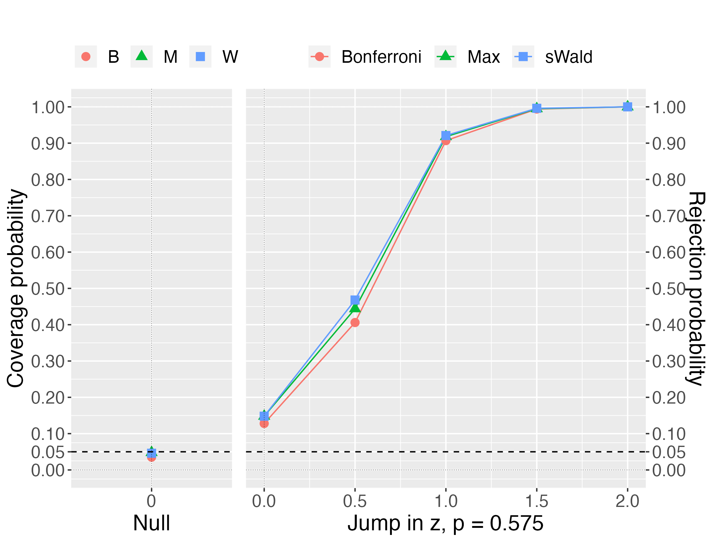
Figure 4: A jump in a scalar $Z$ and a density test, $n=1000$

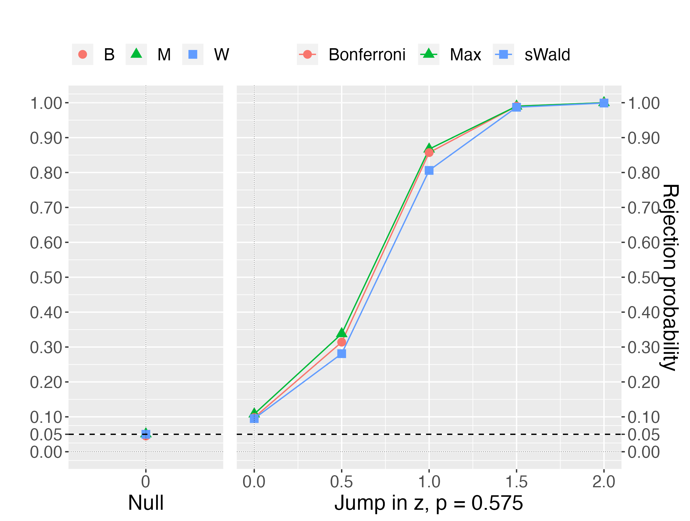
(a) Covariates have the same pairwise correlation coefficient of $0.5$

(b) Covariates have the same pairwise correlation coefficient of $0.9$

Figure 5: A jump in the three covariates with a density, $n=1000$

(a) Covariates have the same pairwise correlation coefficient of $0.5$

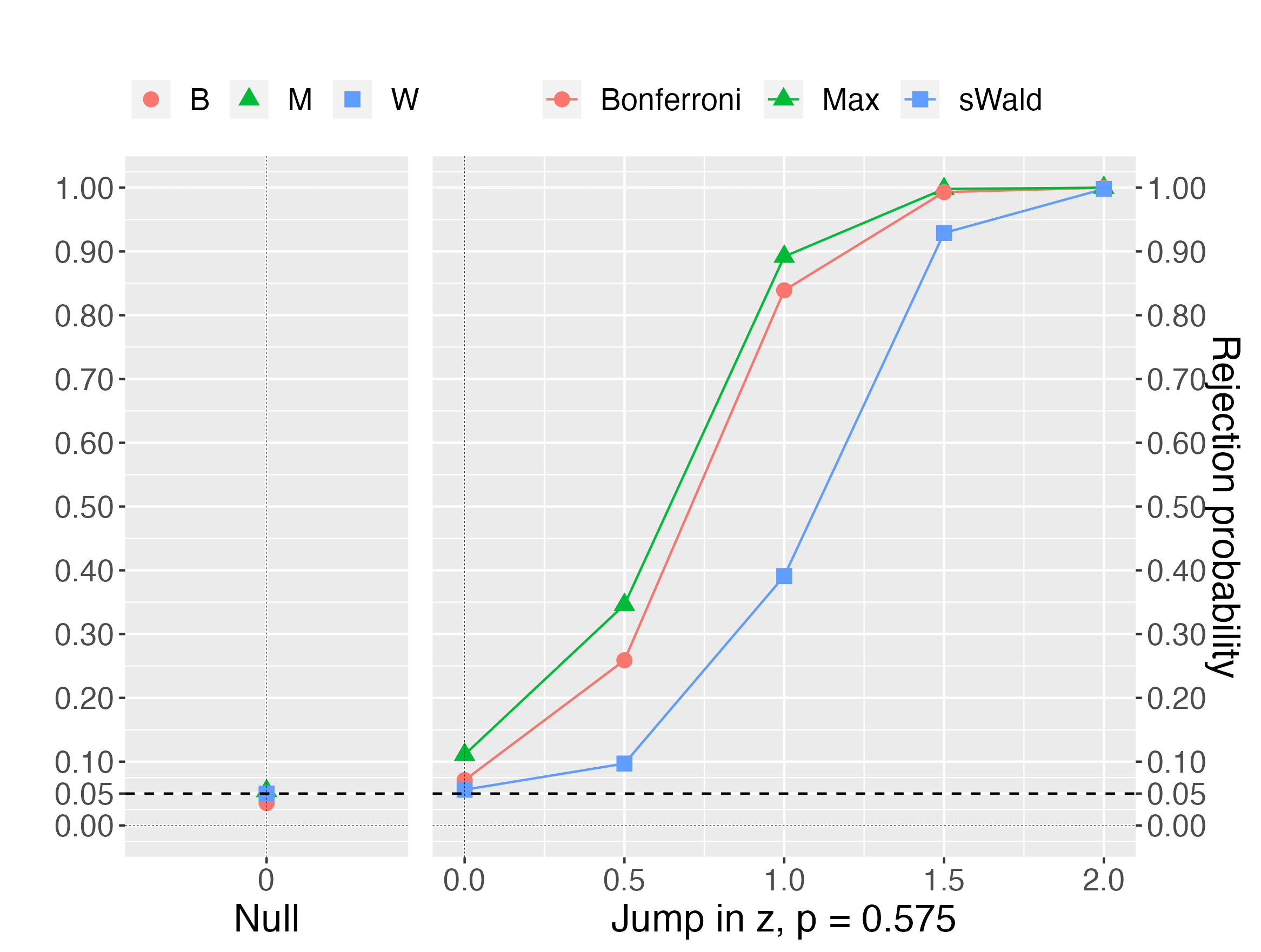
(b) Covariates have the same pairwise correlation coefficient of $0.9$

Figure 6: A jump in the five covariates with a density, $n=1000$

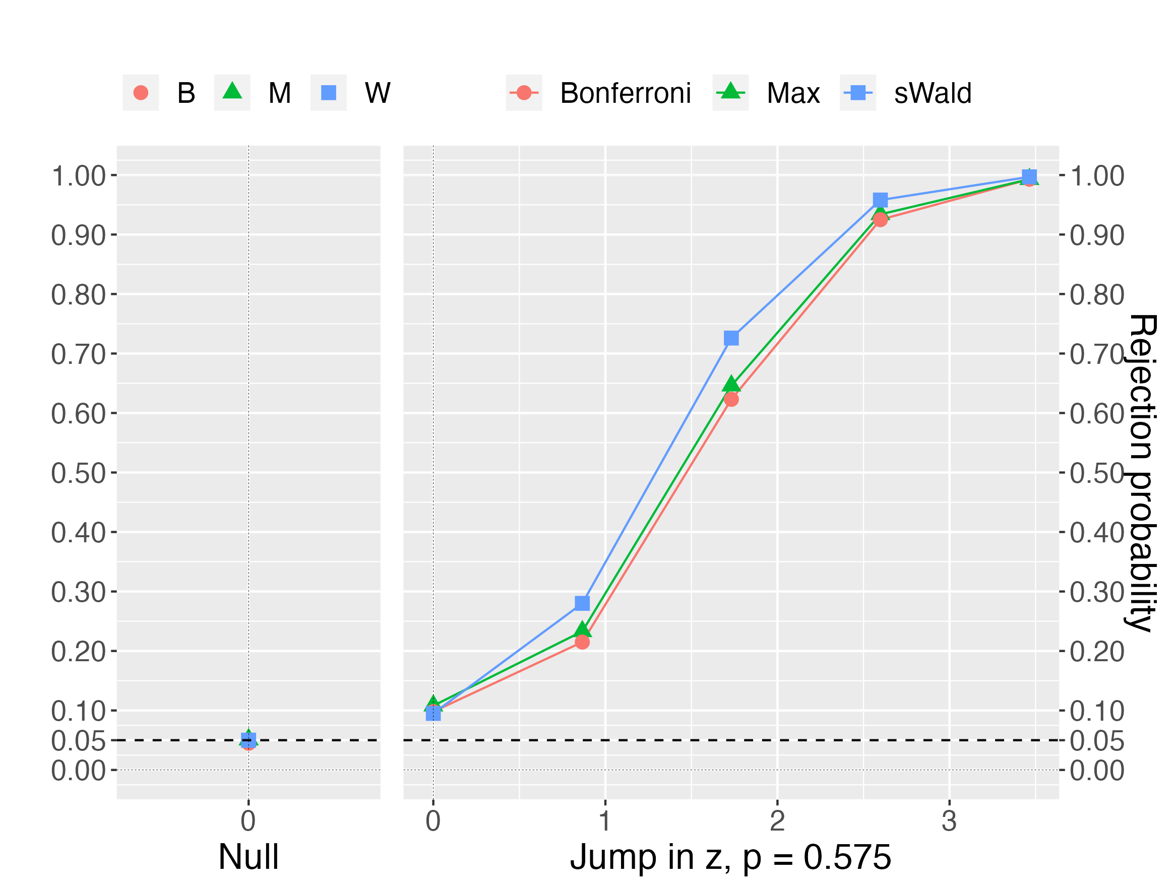
(a) Covariates have the same pairwise correlation coefficient of $0.5$

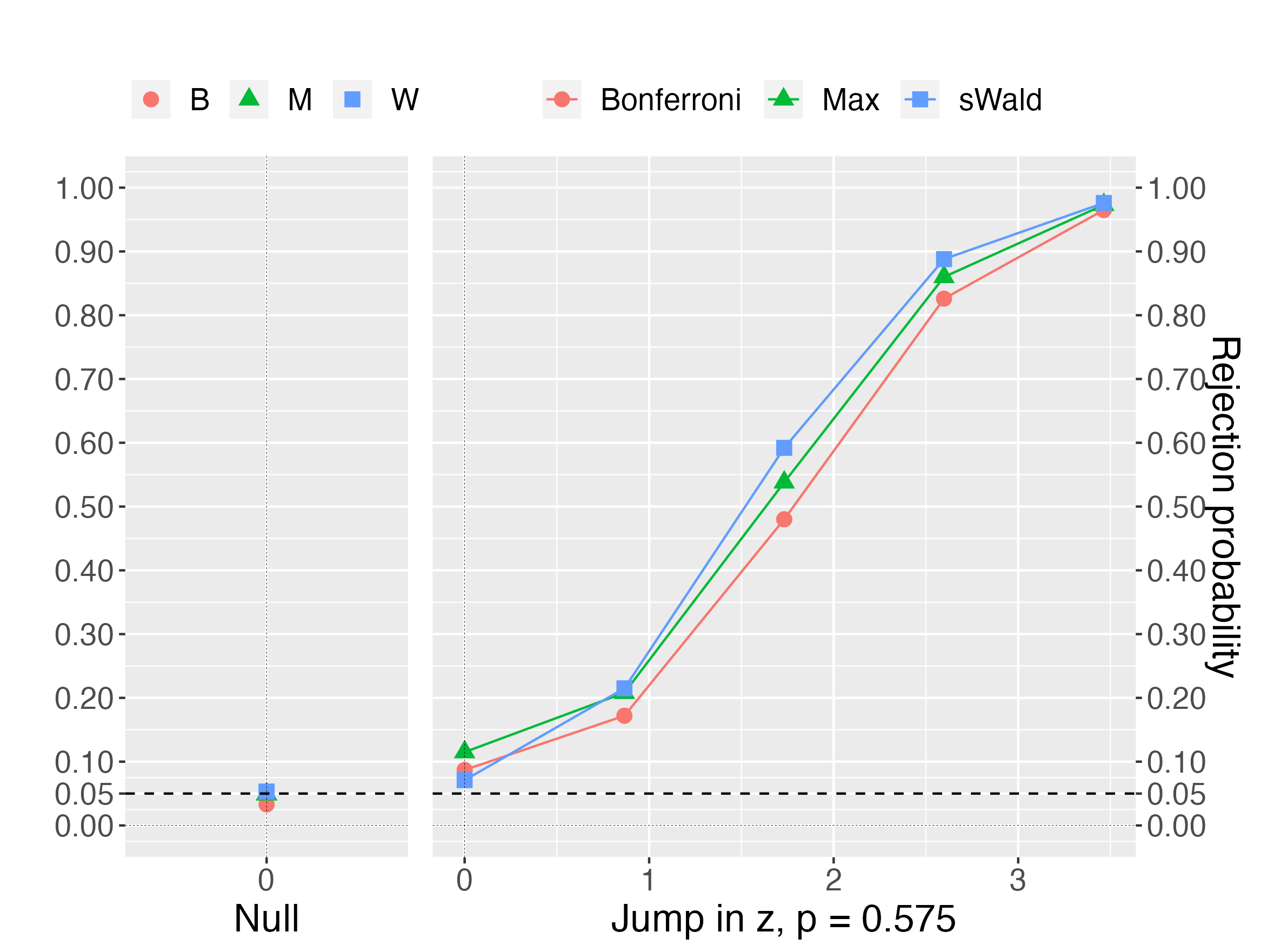
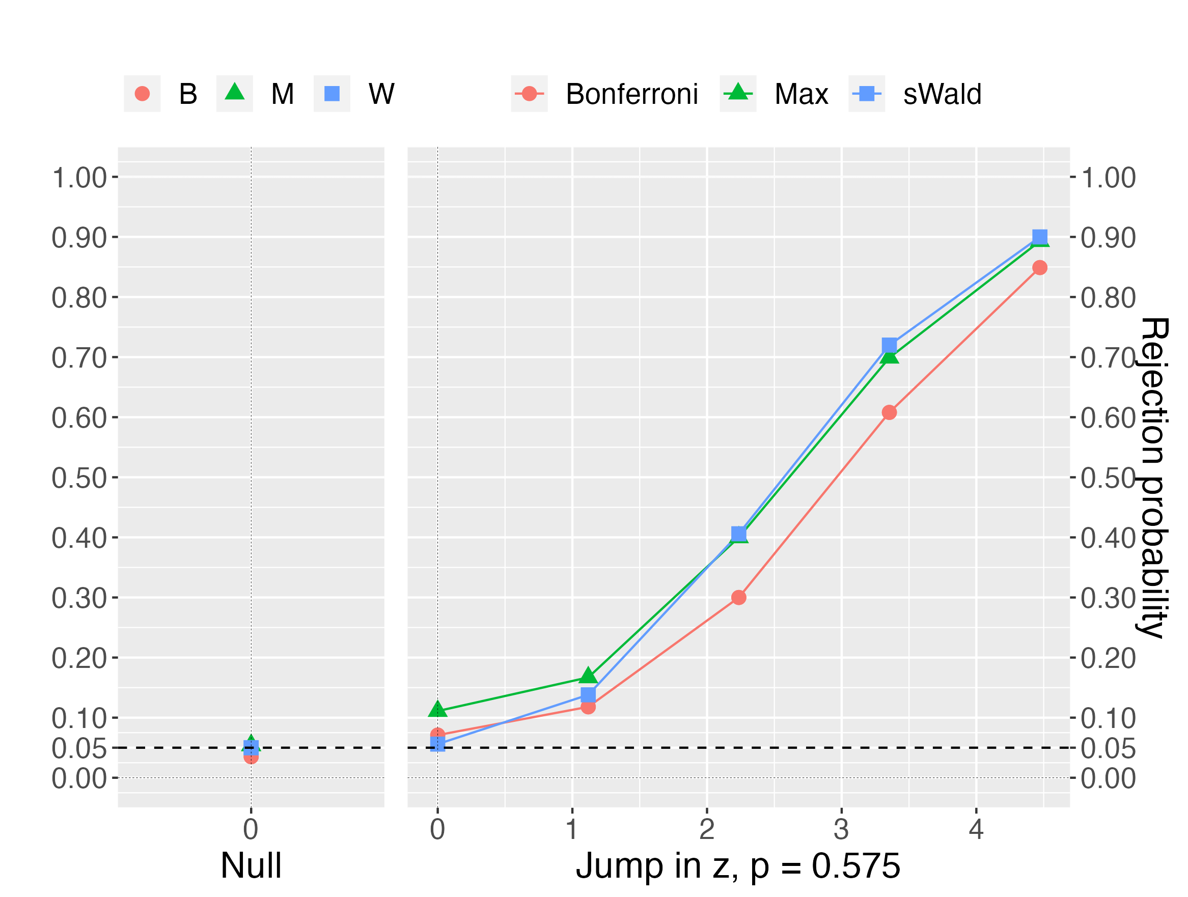
(b) Covariates have the same pairwise correlation coefficient of $0.9$

Figure 7: $1/3$ of jumps in all the three covariates with a density, $n=1000$

(a) Covariates have the same pairwise correlation coefficient of $0.5$

(b) Covariates have the same pairwise correlation coefficient of $0.9$

Figure 8: $1/5$ of jumps in all the five covariates with a density, $n=1000$

Next, we compare the empirical power of the (ii) Bonferroni correction, (iv) Max test, and (v) sWald test under $\bar{p}=0.575$ and $\tau_{Z_{d}}(=a)=0,0.5,1,1.5,2$ for different dimensions $d=1,3,5$. Figure 4 presents the result for a scalar covariate, Figures 5 and 6 present the results when one of the $d$ covariates jumps, and Figures 7 and 8 present the results when all the $d$ covariates jump, but each jump size is divided by $d$ for $d=3,5$. In Figures 5-8, each figure present the results for different correlations $\rho=0.5,0.9$. In all cases, the Max test has more power than the Bonferroni correction. The difference between these methods is more considerable when the correlation is stronger. This finding suggests that the Max test is more robust to strong correlations $\rho$ than the Bonferroni correction. For the first case (Figures 5 and 6), the sWald test becomes more conservative when $d$ or $\rho$ is larger. For the second case (Figures 7 and 8), all the methods become more conservative when $d$ is larger; nevertheless, the sWald test is more robust against larger dimensions $d$, and the sWald test has more power than the Max test when the correlation is milder. In conclusion, both the Max and sWald tests complement each other.

The simulation results show that the proposed joint testing methods exhibit vital size control and power improvements. The Max and sWald tests are more robust against larger dimensions $d$ for size control than the naive and conventional Wald tests. The Max test has a higher power than the Bonferroni correction, which has better size control. The sWald test is almost the best in size control when the sample size is $n=1000$. The sWald test performs better in its power when many covariates have discontinuities; however, the sWald test may perform worse than the Max test or Bonferroni correction when only one of many covariates has a jump. In Appendix D, we report qualitatively similar simulation results of other specifications including lower correlation coefficients and a negative correlation coefficient.

5 Conclusion

Diagnostic tests are vital to applied studies of RD designs; however, inappropriate use of them ruins their purpose. The current practice suffers from the multiple testing problem: a single identifying restriction implies multiple testable restrictions, but these restrictions are tested separately without appropriate size control.

We demonstrated an extraordinary consequence of the multiple testing problem. Among the $60$ papers published in the top-five economics journals, most papers run more than $10$ covariates balance tests, but most studies run these tests separately. Consequently, the rejection probability of the joint null hypothesis is $35\%$, which is an enormous over-rejection relative to the nominal size of $5\%$. Furthermore, we discovered that over-rejection from naive (separate) testing is greater for papers with many covariates. Hence, the current diagnostic procedure is useless in validating the identification assumption.

We provided a resolution for this multiple testing problem. We showed the joint asymptotic normality of the RD design estimators and provided alternative joint testing procedures. We provided two different joint tests; the proposed tests are the standardized Wald (sWald) test and the Max test. In the simulation studies, we demonstrated that both proposed tests attain a nominal size of $5\%$ when the number of covariates is moderate. The former standardized Wald test has higher power against alternative hypotheses that many covariates have discontinuities. The latter Max test has better power properties against alternative hypotheses that only a few covariates have discontinuities. Overall, both proposed tests perform better than the Bonferroni correction.

Consequently, applied researchers should follow either of the following procedures depending on the possible underlying alternative hypotheses. We recommend the Max test when only a few covariates are particularly concerning in violation of local randomization, although other covariates are expected to be continuous. We recommend a standardized Wald test for other designs with no explicit concern. Interestingly, the size control of the tests may not be granted even for the test with Bonferroni correction when the number of covariates is larger than $10$. In other words, the validity of the joint test is not guaranteed with more than $10$ covariates. Hence, we do not recommend running too many balance tests simultaneously if the sample size is moderate.

Based on our findings, we consider several topics for future research. First, finding another use for testable restrictions may be preferable. In validating local randomization, we need to focus on the joint null hypothesis and are not interested in detecting which restrictions fail. Hence, separate tests or other approaches including false discovery rate control are inappropriate. Nevertheless, if we detect a particular subgroup of covariates that invalidate local randomization, such a finding may provide valuable information. Diagnostic procedures with such information may improve design validation. Second, we focus on the statistical inference of the testable restrictions; nonetheless, a graphical analysis of the testable restrictions is important. Recent studies such as Calonico, Cattaneo, and Titiunik (2015) consider the optimal procedure in visualization, and Korting, Lieberman, Matsudaira, Pei, and Shen (2023) demonstrate that tuning parameters in visualization is critical. We recommend our joint testing along with the graphical analysis, and multiple testing problems in graphical analyses can be a future research topic. Finally, we find that jointly testing statistics that are nonparametric estimates is challenging. Although our Max and sWald tests performed better than the Bonferroni correction, a fundamental improvement in the joint test is still desirable. Note that typical improvements over the Bonferroni correction, such as step-up or step-down methods, do not help improve the test for the joint null hypothesis. We will consider these issues as future research questions.

Appendix A Formal results

Appendix A provides formal theoretical results and their proofs.

A.1 Setup and Notation

Let $|\cdot|$ denote the Euclidean matrix norm, that is, $|A|^{2}=\operatorname{trace}(A^{\prime}A)=\sum_{j=1}^{n}\sum_{i=1}^{m}a_{ij}^{2}$ for $(m\times n)$ matrix $A=\{a_{ij}\}_{i=1,\ldots,m}^{j=1,\ldots,n}$, and $|a|^{4}=|aa^{\prime}|^{2}=\sum_{j=1}^{n}\sum_{i=1}^{n}a_{i}^{2}a_{j}^{2}$ for $(n\times 1)$ vector $a=(a_{1},\ldots,a_{n})^{\prime}$. Let $a_{n}\precsim b_{n}$ denote $a_{n}\leq Cb_{n}$ for a positive constant $C$, which is independent of $n$.

The estimands of the local polynomial estimators are

$$\beta_{Z_{k}+,l}=\left[\mu_{Z_{k}+},\frac{\mu_{Z_{k}+}^{(1)}}{1!},\ldots,\frac{\mu_{Z_{k}+}^{(l)}}{l!}\right]^{\prime},\,\,\beta_{Z_{k}-,l}=\left[\mu_{Z_{k}-},\frac{\mu_{Z_{k}-}^{(1)}}{1!},\ldots,\frac{\mu_{Z_{k}-}^{(l)}}{l!}\right]^{\prime},$$

$$\beta_{f+,p}=\left[{F}_{+},\frac{f_{+}}{1!},\frac{f^{(1)}_{+}}{2!},\ldots,\frac{f^{(p-1)}_{+}}{p!}\right]^{\prime},\,\,\beta_{f-,p}=\left[{F}_{-},\frac{f_{-}}{1!},\frac{f^{(1)}_{-}}{2!},\ldots,\frac{f^{(p-1)}_{-}}{p!}\right]^{\prime},$$

where $F(x)=E[1\{X\leq x\}]$, ${F}_{+}=\lim_{x\to 0^{+}}F(x)$, ${F}_{-}=\lim_{x\to 0^{-}}F(x)$.
We set $Z_{k}=(Z_{k,1},\ldots,Z_{k,n})^{\prime}$, $\tilde{F}=(\tilde{F}(X_{1}),\ldots,\tilde{F}(X_{n}))^{\prime}$, $K_{h}(u)=K(u/h)/h$, $H_{p}(h)=\operatorname{diag}(1,h,\ldots,h^{p})$, $X_{p}(h)=[r_{p}(X_{1}/h),\ldots,r_{p}(X_{n}/h)]^{\prime}$,

$$W_{+}(h)=\operatorname{diag}(1\{X_{1}\geq 0\}K_{h}(X_{1}),\ldots,1\{X_{n}\geq 0\}K_{h}(X_{n})),$$

$$W_{-}(h)=\operatorname{diag}(1\{X_{1}<0\}K_{h}(X_{1}),\ldots,1\{X_{n}<0\}K_{h}(X_{n})),$$

$$\Gamma_{+,p}(h)=\frac{1}{n}X_{p}(h)^{\prime}W_{+}(h)X_{p}(h),\quad\Gamma_{-,p}(h)=\frac{1}{n}X_{p}(h)^{\prime}W_{-}(h)X_{p}(h),$$

The local polynomial estimators are

$$\hat{\beta}_{Z_{k}+,l}(h_{k})=\frac{1}{n}H_{l}^{-1}(h_{k})\Gamma_{+,l}^{-1}(h_{k})X_{l}(h_{k})^{\prime}W_{+}(h_{k})Z_{k},$$

$$\hat{\beta}_{Z_{k}-,l}(h_{k})=\frac{1}{n}H_{l}^{-1}(h_{k})\Gamma_{-,l}^{-1}(h_{k})X_{l}(h_{k})^{\prime}W_{-}(h_{k})Z_{k},$$

and

$$\hat{\beta}_{f+,p}(h_{f})=\frac{1}{n}H_{p}^{-1}(h_{f})\Gamma_{+,p}^{-1}(h_{f})X_{p}(h_{f})^{\prime}W_{+}(h_{f})\tilde{F},$$

$$\hat{\beta}_{f-,p}(h_{f})=\frac{1}{n}H_{p}^{-1}(h_{f})\Gamma_{-,p}^{-1}(h_{f})X_{p}(h_{f})^{\prime}W_{-}(h_{f})\tilde{F}.$$

Let

$$\Delta\hat{\mu}_{Z_{k}+,l}(h_{k})\equiv\sqrt{nh_{k}}[\hat{\mu}_{Z_{k}+,l}(h_{k})-{\mu}_{Z_{k}+}],\quad\Delta\hat{\mu}_{Z_{k}-,l}(h_{k})\equiv\sqrt{nh_{k}}[\hat{\mu}_{Z_{k}-,l}(h_{k})-{\mu}_{Z_{k}-}],$$

$$\Delta\hat{f}_{+,p}(h_{f})\equiv\sqrt{nh_{f}}[\hat{f}_{+,p}(h_{f})-f_{+}],\quad\Delta\hat{f}_{-,p}(h_{f})\equiv\sqrt{nh_{f}}[\hat{f}_{-,p}(h_{f})-f_{-}].$$

Letting $\mathcal{X}_{n}=(X_{1},\ldots,X_{n})^{\prime}$, we decompose $\Delta\hat{\mu}_{Z_{k}+,l}(h_{k})$ and $\Delta\hat{\mu}_{Z_{k}-,l}(h_{k})$ as

$$\Delta\hat{\mu}_{Z_{k}+,l}(h_{k})=\Delta^{M}\hat{\mu}_{Z_{k}+,l}(h_{k})+\Delta^{B}\hat{\mu}_{Z_{k}+,l}(h_{k}),$$

$$\Delta\hat{\mu}_{Z_{k}-,l}(h_{k})=\Delta^{M}\hat{\mu}_{Z_{k}-,l}(h_{k})+\Delta^{B}\hat{\mu}_{Z_{k}-,l}(h_{k}),$$

where

$$\Delta^{M}\hat{\mu}_{Z_{k}+,l}(h_{k})\equiv\sqrt{nh_{k}}\{\hat{\mu}_{Z_{k}+,l}(h_{k})-E[\hat{\mu}_{Z_{k}+,l}(h_{k})|\mathcal{X}_{n}]\},$$

$$\Delta^{M}\hat{\mu}_{Z_{k}-,l}(h_{k})\equiv\sqrt{nh_{k}}\{\hat{\mu}_{Z_{k}-,l}(h_{k})-E[\hat{\mu}_{Z_{k}-,l}(h_{k})|\mathcal{X}_{n}]\}$$

and

$$\Delta^{B}\hat{\mu}_{Z_{k}+,l}(h_{k})\equiv\sqrt{nh_{k}}\{E[\hat{\mu}_{Z_{k}+,l}(h_{k})|\mathcal{X}_{n}]-{\mu}_{Z_{k}+}\},$$

$$\Delta^{B}\hat{\mu}_{Z_{k}-,l}(h_{k})\equiv\sqrt{nh_{k}}\{E[\hat{\mu}_{Z_{k}-,l}(h_{k})|\mathcal{X}_{n}]-{\mu}_{Z_{k}-}\}.$$

$\Delta^{B}\hat{\mu}_{Z_{k}+,l}(h_{k})$ and $\Delta^{B}\hat{\mu}_{Z_{k}-,l}(h_{k})$ represent the smoothing bias, and we consider distributional approximations of $\Delta^{M}\hat{\mu}_{Z_{k}+,l}(h_{k})$ and $\Delta^{M}\hat{\mu}_{Z_{k}-,l}(h_{k})$.

We define $\tilde{f}_{+,p}(h_{f})$ and $\tilde{f}_{-,p}(h_{f})$ as the slope coefficients in the following local polynomial regressions:

$$\tilde{f}_{+,p}(h_{f})=e_{1}^{\prime}\tilde{\beta}_{f+,p}(h_{f}),\quad\tilde{f}_{-,p}(h_{f})=e_{1}^{\prime}\tilde{\beta}_{f-,p}(h_{f}),$$

where

$$\tilde{\beta}_{f+,p}(h_{f})=\operatorname*{arg\,min}_{\beta\in\mathbb{R}^{p+1}}\sum_{i=1}^{n}1\{X_{i}\geq 0\}({F}(X_{i})-r_{p}(X_{i})^{\prime}\beta)^{2}{K}_{h_{f}}(X_{i}),$$

$$\tilde{\beta}_{f-,p}(h_{f})=\operatorname*{arg\,min}_{\beta\in\mathbb{R}^{p+1}}\sum_{i=1}^{n}1\{X_{i}<0\}({F}(X_{i})-r_{p}(X_{i})^{\prime}\beta)^{2}{K}_{h_{f}}(X_{i}).$$

$\tilde{f}_{+,p}(h_{f})$ and $\tilde{f}_{-,p}(h_{f})$ are obtained from $p$th-order local polynomial one-sided approximations to the true distribution of $X_{i}$. We decompose $\Delta\hat{f}_{+,p}(h_{f})$ and $\Delta\hat{f}_{-,p}(h_{f})$ as

$$\Delta\hat{f}_{+,p}(h_{f})=\Delta^{M_{0}}\hat{f}_{+,p}(h_{f})+\Delta^{B_{0}}\hat{f}_{+,p}(h_{f}),\quad\Delta\hat{f}_{-,p}(h_{f})=\Delta^{M_{0}}\hat{f}_{-,p}(h_{f})+\Delta^{B_{0}}\hat{f}_{-,p}(h_{f}),$$

where

$$\Delta^{M_{0}}\hat{f}_{+,p}(h_{f})\equiv\sqrt{nh_{f}}\{\hat{f}_{+,p}(h_{f})-\tilde{f}_{+,p}(h_{f})\},$$

$$\Delta^{M_{0}}\hat{f}_{-,p}(h_{f})\equiv\sqrt{nh_{f}}\{\hat{f}_{-,p}(h_{f})-\tilde{f}_{-,p}(h_{f})\}$$

and

$$\Delta^{B_{0}}\hat{f}_{+,p}(h_{f})\equiv\sqrt{nh_{f}}\{\tilde{f}_{+,p}(h_{f})-f_{+}\},\quad\Delta^{B_{0}}\hat{f}_{-,p}(h_{f})\equiv\sqrt{nh_{f}}\{\tilde{f}_{-,p}(h_{f})-f_{-}\}.$$

$\Delta^{B_{0}}\hat{f}_{+,p}(h_{f})$ and $\Delta^{B_{0}}\hat{f}_{-,p}(h_{f})$ represent the smoothing bias. We set
$F=({F}(X_{1}),\ldots,{F}(X_{n}))^{\prime}$, $\iota=(1,\ldots,1)^{\prime}$ that is $n$-dimensional,

$$U_{+,p}(h_{f})\equiv\frac{1}{n(n-1)}\sum_{i,j:i\neq j}^{n}\psi_{+,p,h_{f}}(X_{i},X_{j}),$$

$$U_{-,p}(h_{f})\equiv\frac{1}{n(n-1)}\sum_{i,j:i\neq j}^{n}\psi_{-,p,h_{f}}(X_{i},X_{j}),$$

where

$$\psi_{+,p,h_{f}}(X_{i},X_{j})\equiv 1\{X_{i}\geq 0\}r_{p}(X_{i}/h_{f})(1\{X_{j}\leq X_{i}\}-F(X_{i})){K}_{h_{f}}(X_{i}),$$

$$\psi_{-,p,h_{f}}(X_{i},X_{j})\equiv 1\{X_{i}<0\}r_{p}(X_{i}/h_{f})(1\{X_{j}\leq X_{i}\}-F(X_{i})){K}_{h_{f}}(X_{i}).$$

We further decompose $\Delta^{M_{0}}\hat{f}_{+,p}(h_{f})$ and $\Delta^{M_{0}}\hat{f}_{-,p}(h_{f})$ as

$$\Delta^{M_{0}}\hat{f}_{+,p}(h_{f})=\Delta^{M_{1}}\hat{f}_{+,p}(h_{f})+\Delta^{B_{1}}\hat{f}_{+,p}(h_{f}),$$

$$\Delta^{M_{0}}\hat{f}_{-,p}(h_{f})=\Delta^{M_{1}}\hat{f}_{-,p}(h_{f})+\Delta^{B_{1}}\hat{f}_{-,p}(h_{f}),$$

where

$$\Delta^{M_{1}}\hat{f}_{+,p}(h_{f})\equiv\left(1-\frac{1}{n}\right)\sqrt{\frac{n}{h_{f}}}e_{1}^{\prime}\Gamma_{+,p}^{-1}(h_{f})U_{+,p}(h_{f}),$$

$$\Delta^{M_{1}}\hat{f}_{-,p}(h_{f})\equiv\left(1-\frac{1}{n}\right)\sqrt{\frac{n}{h_{f}}}e_{1}^{\prime}\Gamma_{-,p}^{-1}(h_{f})U_{-,p}(h_{f}),$$

and

$$\Delta^{B_{1}}\hat{f}_{+,p}(h_{f})\equiv\frac{1}{\sqrt{nh_{f}}}\frac{1}{n}e_{1}^{\prime}\Gamma_{+,p}^{-1}(h_{f})X_{p}(h_{f})^{\prime}W_{+}(h_{f})(\iota-{F}),$$

$$\Delta^{B_{1}}\hat{f}_{-,p}(h_{f})\equiv\frac{1}{\sqrt{nh_{f}}}\frac{1}{n}e_{1}^{\prime}\Gamma_{-,p}^{-1}(h_{f})X_{p}(h_{f})^{\prime}W_{-}(h_{f})(\iota-{F}).$$

$U_{+,p}(h_{f})$ and $U_{-,p}(h_{f})$ are regarded as second order U-statistics (where the kernels $\psi_{+,p,h_{f}}(X_{i},X_{j})$ and $\psi_{+,p,h_{f}}(X_{i},X_{j})$ are $(p+1)$-dimensional and depend on the bandwidth $h_{f}$), and $\Delta^{B_{1}}\hat{f}_{+,p}(h_{f})$ and $\Delta^{B_{1}}\hat{f}_{-,p}(h_{f})$ represent the leave-in bias. These terms arise because the empirical distribution function $\tilde{F}(X_{i})$ is approximated, which leads to double summation. Note that $E[\psi_{+,p,h_{f}}(X_{i},X_{j})]=0$, $E[\psi_{-,p,h_{f}}(X_{i},X_{j})]=0$, and it is well known that U-statistics can be decomposed as

$$U_{+,p}(h_{f})=U_{1,+,p}(h_{f})+U_{2,+,p}(h_{f}),\quad U_{-,p}(h_{f})=U_{1,-,p}(h_{f})+U_{2,-,p}(h_{f})$$

with

$$U_{1,+,p}(h_{f})\equiv\frac{1}{n}\sum_{i=1}^{n}E[\psi_{+,p,h_{f}}(X_{j},X_{i})|X_{i}],\quad U_{1,-,p}(h_{f})\equiv\frac{1}{n}\sum_{i=1}^{n}E[\psi_{-,p,h_{f}}(X_{j},X_{i})|X_{i}]$$

for $j\neq i$ and

$$U_{2,+,p}(h_{f})\equiv\frac{1}{n(n-1)}\sum_{i,j:i\neq j}^{n}\varphi_{+,p,h_{f}}(X_{i},X_{j}),$$

$$U_{2,-,p}(h_{f})\equiv\frac{1}{n(n-1)}\sum_{i,j:i\neq j}^{n}\varphi_{-,p,h_{f}}(X_{i},X_{j}),$$

where

$$\begin{split}\varphi_{+,p,h_{f}}(X_{i},X_{j})\equiv&\psi_{+,p,h_{f}}(X_{i},X_{j})+\psi_{+,p,h_{f}}(X_{j},X_{i})\\ &-E[\psi_{+,p,h_{f}}(X_{i},X_{j})|X_{j}]-E[\psi_{+,p,h_{f}}(X_{j},X_{i})|X_{i}],\end{split}$$

$$\begin{split}\varphi_{-,p,h_{f}}(X_{i},X_{j})\equiv&\psi_{-,p,h_{f}}(X_{i},X_{j})+\psi_{-,p,h_{f}}(X_{j},X_{i})\\ &-E[\psi_{-,p,h_{f}}(X_{i},X_{j})|X_{j}]-E[\psi_{-,p,h_{f}}(X_{j},X_{i})|X_{i}].\end{split}$$

This decomposition is often referred to as Hoeffding’s decomposition (see, for example, Serfling (1980)). $U_{2,+,p}(h_{f})$ and $U_{2,-,p}(h_{f})$ are degenerate U-statistics, and it is shown later that they are asymptotically negligible under our assumptions. Let

$$\Delta^{B_{2}}\hat{f}_{+,p}(h_{f})\equiv\sqrt{\frac{n}{h_{f}}}e_{1}^{\prime}\Gamma_{+,p}^{-1}(h_{f})U_{2,+,p}(h_{f}),$$

$$\Delta^{B_{2}}\hat{f}_{-,p}(h_{f})\equiv\sqrt{\frac{n}{h_{f}}}e_{1}^{\prime}\Gamma_{-,p}^{-1}(h_{f})U_{2,-,p}(h_{f}),$$

$$\Delta^{B_{3}}\hat{f}_{+,p}(h_{f})\equiv-\frac{1}{\sqrt{nh_{f}}}e_{1}^{\prime}\Gamma_{+,p}^{-1}(h_{f})U_{+,p}(h_{f}),$$

$$\Delta^{B_{3}}\hat{f}_{-,p}(h_{f})\equiv-\frac{1}{\sqrt{nh_{f}}}e_{1}^{\prime}\Gamma_{-,p}^{-1}(h_{f})U_{-,p}(h_{f}),$$

and we can decompose $\Delta\hat{f}_{+,p}(h_{f})$ and $\Delta\hat{f}_{-,p}(h_{f})$ into

$$\Delta\hat{f}_{+,p}(h_{f})=\Delta^{M}\hat{f}_{+,p}(h_{f})+\Delta^{B}\hat{f}_{+,p}(h_{f}),\quad\Delta\hat{f}_{-,p}(h_{f})=\Delta^{M}\hat{f}_{-,p}(h_{f})+\Delta^{B}\hat{f}_{-,p}(h_{f}),$$

where

$$\Delta^{M}\hat{f}_{+,p}(h_{f})\equiv\sqrt{\frac{n}{h_{f}}}e_{1}^{\prime}\Gamma_{+,p}^{-1}(h_{f})U_{1,+,p}(h_{f}),\quad\Delta^{M}\hat{f}_{-,p}(h_{f})\equiv\sqrt{\frac{n}{h_{f}}}e_{1}^{\prime}\Gamma_{-,p}^{-1}(h_{f})U_{1,-,p}(h_{f})$$

and

$$\Delta^{B}\hat{f}_{+,p}(h_{f})\equiv\sum_{j=0}^{3}\Delta^{B_{j}}\hat{f}_{+,p}(h_{f}),\quad\Delta^{B}\hat{f}_{-,p}(h_{f})\equiv\sum_{j=0}^{3}\Delta^{B_{j}}\hat{f}_{-,p}(h_{f}).$$

we consider distributional approximations of $\Delta^{M}\hat{f}_{+,p}(h_{f})$ and $\Delta^{M}\hat{f}_{-,p}(h_{f})$.

To characterize the bias and variance of the local polynomial estimators, we also employ the following notation:

$$\sigma^{2}_{Z_{k}+}=\lim_{x\to 0^{+}}\sigma^{2}_{Z_{k}}(x),\quad\sigma^{2}_{Z_{k}-}=\lim_{x\to 0^{-}}\sigma^{2}_{Z_{k}}(x),\quad\sigma^{2}_{Z_{k}}(x)=\operatorname{Var}(Z_{k}|X=x),$$

$$\sigma_{Z_{j}Z_{k}+}=\lim_{x\to 0^{+}}\sigma_{Z_{j}Z_{k}}(x),\quad\sigma_{Z_{j}Z_{k}-}=\lim_{x\to 0^{-}}\sigma_{Z_{j}Z_{k}}(x),\quad\sigma_{Z_{j}Z_{k}}(x)=\operatorname{Cov}(Z_{j},Z_{k}|X=x),$$

$\varepsilon_{Z_{k}}=(\varepsilon_{Z_{k},1},\ldots,\varepsilon_{Z_{k},n})^{\prime}$ with $\varepsilon_{Z_{k},i}=Z_{k,i}-\mu_{Z_{k}}(X_{i})$,

$$\Sigma_{Z_{k}}=E[\varepsilon_{Z_{k}}\varepsilon_{Z_{k}}^{\prime}|\mathcal{X}_{n}]=\operatorname{diag}(\sigma^{2}_{Z_{k}}(X_{1}),\ldots,\sigma^{2}_{Z_{k}}(X_{n})),$$

$$\Sigma_{Z_{j}Z_{k}}=E[\varepsilon_{Z_{j}}\varepsilon_{Z_{k}}^{\prime}|\mathcal{X}_{n}]=\operatorname{diag}(\sigma_{Z_{j}Z_{k}}(X_{1}),\ldots,\sigma_{Z_{j}Z_{k}}(X_{n})),$$

$$S_{p}(h)=[(X_{1}/h)^{p},\ldots,(X_{n}/h)^{p}]^{\prime},$$

$$\vartheta_{+,p,q}(h)=X_{p}(h)^{\prime}W_{+}(h)S_{q}(h)/n,\quad\vartheta_{-,p,q}(h)=X_{p}(h)^{\prime}W_{-}(h)S_{q}(h)/n,$$

$$\Psi_{Z_{j}Z_{k}+,p,q}(h_{j},h_{k})=X_{p}(h_{j})^{\prime}W_{+}(h_{j})\Sigma_{Z_{j}Z_{k}}W_{+}(h_{k})X_{q}(h_{k})/n,$$

$$\Psi_{Z_{j}Z_{k}-,p,q}(h_{j},h_{k})=X_{p}(h_{j})^{\prime}W_{-}(h_{j})\Sigma_{Z_{j}Z_{k}}W_{-}(h_{k})X_{q}(h_{k})/n,$$

$$\Psi_{Z_{k}+,p}(h)=\Psi_{Z_{k}Z_{k}+,p,p}(h,h)=X_{p}(h)^{\prime}W_{+}(h)\Sigma_{Z_{k}}W_{+}(h)X_{p}(h)/n,$$

$$\Psi_{Z_{k}-,p}(h)=\Psi_{Z_{k}Z_{k}-,p,p}(h,h)=X_{p}(h)^{\prime}W_{-}(h)\Sigma_{Z_{k}}W_{-}(h)X_{p}(h)/n,$$

$$\begin{split}&\tilde{\Psi}_{Z_{j}Z_{k}+,p,q}(h_{j},h_{k})\\ =&\int_{0}^{\infty}K\left(\frac{h_{jk}u}{h_{j}}\right)K\left(\frac{h_{jk}u}{h_{k}}\right)r_{p}\left(\frac{h_{jk}u}{h_{j}}\right)r_{q}\left(\frac{h_{jk}u}{h_{k}}\right)^{\prime}\sigma^{2}_{Z_{j}Z_{k}}(uh_{jk})f(uh_{jk})du,\end{split}$$

$$\begin{split}&\tilde{\Psi}_{Z_{j}Z_{k}-,p,q}(h_{j},h_{k})\\ =&\int_{0}^{\infty}K\left(\frac{h_{jk}u}{h_{j}}\right)K\left(\frac{h_{jk}u}{h_{k}}\right)r_{p}\left(\frac{h_{jk}u}{h_{j}}\right)r_{q}\left(\frac{h_{jk}u}{h_{k}}\right)^{\prime}\sigma^{2}_{Z_{j}Z_{k}}(-uh_{jk})f(-uh_{jk})du,\end{split}$$

$$\tilde{\Psi}_{Z_{k}+,p}(h)=\tilde{\Psi}_{Z_{k}Z_{k}+,p,p}(h,h)=\int_{0}^{\infty}K(u)^{2}r_{p}(u)r_{p}(u)^{\prime}\sigma^{2}_{Z_{k}}(uh)f(uh)du,$$

$$\tilde{\Psi}_{Z_{k}-,p}(h)=\tilde{\Psi}_{Z_{k}Z_{k}-,p,p}(h,h)=\int_{0}^{\infty}K(u)^{2}r_{p}(u)r_{p}(u)^{\prime}\sigma^{2}_{Z_{k}}(-uh)f(-uh)du,$$

$$\Gamma_{p}=\int_{0}^{\infty}K(u)r_{p}(u)r_{p}(u)^{\prime}du,\quad\vartheta_{p,q}=\int_{0}^{\infty}K(u)u^{q}r_{p}(u)du,$$

where $h_{jk}=(h_{j}h_{k})^{1/2}$,

$$\begin{split}&\Psi_{jk,p,q}\\ &=\begin{cases}\int_{0}^{\infty}K\left((c_{jk})^{1/2}u\right)K\left((c_{jk})^{-1/2}u\right)r_{p}\left((c_{jk})^{1/2}u\right)r_{q}\left((c_{jk})^{-1/2}u\right)^{\prime}du&\text{if }\rho_{jk}\to c_{jk}\\ 0&\text{otherwise}\end{cases}\\ &=\begin{cases}(c_{jk})^{1/2}\int_{0}^{\infty}K\left(c_{jk}u\right)K\left(u\right)r_{p}\left(c_{jk}u\right)r_{q}\left(u\right)^{\prime}du&\text{if }\rho_{jk}\to c_{jk}\\ 0&\text{otherwise},\end{cases}\end{split}$$

for $c_{jk}\in(0,\infty)$,

$$\Psi_{p,q}=\Psi_{kk,p,q}=\int_{0}^{\infty}K(u)^{2}r_{p}(u)r_{q}(u)^{\prime}du,$$

$$\Psi_{f,p}=\int_{0}^{\infty}\int_{0}^{\infty}(u\wedge v)r_{p}(u)r_{p}(v)^{\prime}K(u)K(v)dudv.$$

A.2 Preliminary Lemmas

First, we provide the asymptotic bias, variance, and distribution of local polynomial estimators. We provide the proofs of the Lemmas in Appendix A.4.

The following lemma provides asymptotic behavior of the bias terms for the local polynomial estimators:

Lemma 1.

Suppose Assumptions 1-2 hold with $S\geq l+2$ and $\alpha\geq p$.

1. If $nh_{min}\to\infty$ and $h_{max}\to 0$, then

   $$\Delta^{B}\hat{\mu}_{Z_{k}+,l}(h_{k})=\sqrt{n}(h_{k})^{3/2+l}B_{Z_{k}+,l}(h_{k})[1+o_{p}(1)],$$ (A.1)

   $$\Delta^{B}\hat{\mu}_{Z_{k}-,l}(h_{k})=\sqrt{n}(h_{k})^{3/2+l}B_{Z_{k}-,l}(h_{k})[1+o_{p}(1)],$$ (A.2)

   where

   $$B_{Z^{k}+,l}(h_{k})=\frac{\mu^{(l+1)}_{Z_{k}+}}{(l+1)!}\mathcal{B}_{+,0,l,l+1}(h_{k}),\quad B_{Z^{k}-,l}(h_{k})=\frac{\mu^{(l+1)}_{Z_{k}-}}{(l+1)!}\mathcal{B}_{-,0,l,l+1}(h_{k}),$$ (A.3)

   $$\mathcal{B}_{+,s,l,r}(h_{k})=s!e_{s}^{\prime}\Gamma_{+,l}^{-1}(h_{k})\vartheta_{+,l,r}(h_{k})=s!e_{s}^{\prime}\Gamma_{l}^{-1}\vartheta_{l,r}+o_{p}(1),$$ (A.4)

   $$\mathcal{B}_{-,s,l,r}(h_{k})=s!e_{s}^{\prime}\Gamma_{-,l}^{-1}(h_{k})\vartheta_{-,l,r}(h_{k})=(-1)^{s+r}s!e_{s}^{\prime}\Gamma_{l}^{-1}\vartheta_{l,r}+o_{p}(1).$$ (A.5)

2. If $nh_{f}\to\infty$ and $h_{f}\to 0$, then

   $$\Delta^{B_{0}}\hat{f}_{+,p}(h_{f})=\sqrt{n}h^{p+1/2}_{f}B_{f,+,p}(h_{f})[1+o_{p}(1)],\quad\Delta^{B_{1}}\hat{f}_{+,p}(h_{f})=o_{p}(1),$$ (A.6)

   $$\Delta^{B_{0}}\hat{f}_{-,p}(h_{f})=\sqrt{n}h^{p+1/2}_{f}B_{f,-,p}(h_{f})[1+o_{p}(1)],\quad\Delta^{B_{1}}\hat{f}_{-,p}(h_{f})=O_{p}((nh_{f})^{-1/2}),$$ (A.7)

   where

   $$B_{f,+,p}(h_{f})=\frac{f_{+}^{(p)}}{(p+1)!}\mathcal{B}_{+,1,p,p+1}(h_{f}),\quad B_{f,-,p}(h_{f})=\frac{f_{-}^{(p)}}{(p+1)!}\mathcal{B}_{-,1,p,p+1}(h_{f}).$$ (A.8)

3. If $nh_{f}^{2}\to\infty$ and $h_{f}\to 0$, then

   $$\Delta^{B_{2}}\hat{f}_{+,p}(h_{f})=O_{p}((nh_{f}^{2})^{-1/2})=o_{p}(1),\quad\Delta^{B_{2}}\hat{f}_{-,p}(h_{f})=O_{p}((nh_{f}^{2})^{-1/2}).$$ (A.9)

Observe that

$$\Delta^{M}\hat{\mu}_{Z_{k}+,l}(h_{k})=\sqrt{\frac{h_{k}}{n}}e_{0}^{\prime}\Gamma_{+,l}^{-1}(h_{k})X_{l}(h_{k})^{\prime}W_{+}(h_{k})\varepsilon_{Z_{k}},$$

$$\Delta^{M}\hat{\mu}_{Z_{k}-,l}(h_{k})=\sqrt{\frac{h_{k}}{n}}e_{0}^{\prime}\Gamma_{-,l}^{-1}(h_{k})X_{l}(h_{k})^{\prime}W_{-}(h_{k})\varepsilon_{Z_{k}}.$$

The following lemma is used for deriving the asymptotic variance of the local polynomial estimators:

Lemma 2.

Suppose Assumptions 1-2 hold with $S\geq l+2$ and $\alpha\geq p$.

1. If $nh_{min}\to\infty$ and $h_{max}\to 0$, then

   $$\begin{split}&\operatorname{Cov}\left(\sqrt{\frac{h_{j}}{n}}X_{l}(h_{j})^{\prime}W_{+}(h_{j})\varepsilon_{Z_{j}},\sqrt{\frac{h_{k}}{n}}X_{l}(h_{k})^{\prime}W_{+}(h_{k})\varepsilon_{Z_{k}}\right)\\ =&f_{+}\sigma_{Z_{j}Z_{k}+}\Psi_{jk,l,l}+o(1)\end{split}$$

   and

   $$\begin{split}&\operatorname{Cov}\left(\sqrt{\frac{h_{j}}{n}}X_{l}(h_{j})^{\prime}W_{-}(h_{j})\varepsilon_{Z_{j}},\sqrt{\frac{h_{k}}{n}}X_{l}(h_{k})^{\prime}W_{-}(h_{k})\varepsilon_{Z_{k}}\right)\\ =&f_{-}\sigma_{Z_{j}Z_{k}-}H_{l}(-1)\Psi_{jk,l,l}H_{l}(-1)+o(1).\end{split}$$

2. If $nh_{f}^{2}\to\infty$ and $h_{f}\to 0$, then

   $$\operatorname{Var}\left(\sqrt{\frac{n}{h_{f}}}U_{1,+,p}(h_{f})\right)$$

   $$= \frac{1}{h_{f}}f_{+}^{2}(F_{+}-F_{+}^{2})\Gamma_{p}e_{0}e_{0}^{\prime}\Gamma_{p}+f_{+}^{3}\Psi_{f,p}$$

   $$+\{-f_{+}^{3}F_{+}+f_{+}f^{\prime}_{+}(F_{+}-F_{+}^{2})\}\Gamma_{p}(e_{1}e_{0}^{\prime}+e_{0}e_{1}^{\prime})\Gamma_{p}+o(1)$$

   and

   $$\operatorname{Var}\left(\sqrt{\frac{n}{h_{f}}}U_{1,-,p}(h_{f})\right)$$

   $$= \frac{1}{h_{f}}f_{-}^{2}(F_{-}-F_{-}^{2})H_{p}(-1)\Gamma_{p}e_{0}e_{0}^{\prime}\Gamma_{p}H_{p}(-1)+f_{-}^{3}H_{p}(-1)\Psi_{f,p}H_{p}(-1)$$

   $$-\{-f_{-}^{3}(F_{-}-1)+f_{-}f^{\prime}_{-}(F_{-}-F_{-}^{2})\}H_{p}(-1)\Gamma_{p}(e_{1}e_{0}^{\prime}+e_{0}e_{1}^{\prime})\Gamma_{p}H_{p}(-1)$$

   $$+o(1).$$

3. $$\operatorname{Cov}\left(X_{l}(h_{k})^{\prime}W_{+}(h_{k})\varepsilon_{Z_{k}},U_{1,+,p}(h_{f})\right)=0$$

   and

   $$\operatorname{Cov}\left(X_{l}(h_{k})^{\prime}W_{-}(h_{k})\varepsilon_{Z_{k}},U_{1,-,p}(h_{f})\right)=0.$$

We set

$$C_{Z_{j}Z_{k}+,l}=\frac{\sigma^{2}_{Z_{j}Z_{k}+}}{f_{+}}e_{0}^{\prime}\Gamma_{l}^{-1}\Psi_{jk,l,l}\Gamma_{l}^{-1}e_{0},\quad C_{Z_{j}Z_{k}-,l}=\frac{\sigma^{2}_{Z_{j}Z_{k}-}}{f_{-}}e_{0}^{\prime}\Gamma_{l}^{-1}\Psi_{jk,l,l}\Gamma_{l}^{-1}e_{0},$$

$$V_{Z_{k}+,l}=C_{Z_{k}Z_{k}+,l}=\frac{\sigma^{2}_{Z_{k}+}}{f_{+}}e_{0}^{\prime}\Gamma_{l}^{-1}\Psi_{l}\Gamma_{l}^{-1}e_{0},\quad V_{Z_{k}-,l}=C_{Z_{k}Z_{k}-,l}=\frac{\sigma^{2}_{Z_{k}-}}{f_{-}}e_{0}^{\prime}\Gamma_{l}^{-1}\Psi_{l}\Gamma_{l}^{-1}e_{0},$$

$$V_{f,+,p}=f_{+}e_{1}^{\prime}\Gamma^{-1}_{p}\Psi_{f,p}\Gamma^{-1}_{p}e_{1},\quad V_{f,-,p}=f_{-}e_{1}^{\prime}\Gamma^{-1}_{p}\Psi_{f,p}\Gamma^{-1}_{p}e_{1}.$$

With Lemmas 1 and 2 at hand, the following lemma provides the asymptotic distribution for the local polynomial estimators:

Lemma 3.

Suppose Assumptions 1-2 hold with $S\geq l+2$ and $\alpha\geq p$. If $nh_{min}\to\infty$, $nh_{f}^{2}\to\infty$, $n(h_{max})^{2l+3}\to 0$, and $n(h_{f})^{2p+1}\to 0$, then

$$[\Delta\hat{\mu}_{Z_{1}+,l}(h_{1}),\ldots,\Delta\hat{\mu}_{Z_{d}+,l}(h_{d}),\Delta\hat{f}_{+,p}(h_{f})]^{\prime}\stackrel{{\scriptstyle d}}{{\to}}N_{d+1}(0,V_{+,l,p}),$$ (A.10)

$$[\Delta\hat{\mu}_{Z_{1}-,l}(h_{1}),\ldots,\Delta\hat{\mu}_{Z_{d}-,l}(h_{d}),\Delta\hat{f}_{-,p}(h_{f})]^{\prime}\stackrel{{\scriptstyle d}}{{\to}}N_{d+1}(0,V_{-,l,p}),$$ (A.11)

where

$$V_{+,l,p}=\begin{pmatrix}V_{Z_{+},l}&0\\ 0&V_{f,+,p}\end{pmatrix},\quad V_{Z+,l}=\{C_{Z_{j}Z_{k}+,l}\}_{j,k=1,\ldots,d},$$

$$V_{-,l,p}=\begin{pmatrix}V_{Z_{-},l}&0\\ 0&V_{f,-,p}\end{pmatrix},\quad V_{Z-,l}=\{C_{Z_{j}Z_{k}-,l}\}_{j,k=1,\ldots,d}.$$

Remark 3.

In Lemma 2 (b), the results for the left-side and right-side estimators are not analogous. The term

$$\{-f_{+}^{3}F_{+}+f_{+}f^{\prime}_{+}(F_{+}-F_{+}^{2})\}\Gamma_{p}(e_{1}e_{0}^{\prime}+e_{0}e_{1}^{\prime})\Gamma_{p}$$

for the right-side estimator changes to

$$-\{-f_{-}^{3}(F_{-}-1)+f_{-}f^{\prime}_{-}(F_{-}-F_{-}^{2})\}H_{p}(-1)\Gamma_{p}(e_{1}e_{0}^{\prime}+e_{0}e_{1}^{\prime})\Gamma_{p}H_{p}(-1)$$

for the left-side estimator. Nevertheless, observe that

$$e_{1}^{\prime}\Gamma_{p}^{-1}\Gamma_{p}(e_{1}e_{0}^{\prime}+e_{0}e_{1}^{\prime})\Gamma_{p}\Gamma_{p}^{-1}e_{1}=e_{1}^{\prime}(e_{1}e_{0}^{\prime}+e_{0}e_{1}^{\prime})e_{1}=0,$$

and the difference has no effect on the whole asymptotic variances $V_{f,+,p}$ and $V_{f,-,p}$. We outline the proof of Lemma 2 (b) for the left-side estimator in Remark 4.

A.3 Asymptotic covariance matrix and standard error estimation

Using the asymptotic covariance matrices of $(\hat{\mu}_{Z_{1}+,l}(h_{1}),\ldots,\hat{\mu}_{Z_{d}+,l}(h_{d}),\hat{f}_{+,p}(h_{f}))^{\prime}$ and $(\hat{\mu}_{Z_{1}-,l}(h_{1}),\ldots,\hat{\mu}_{Z_{d}-,l}(h_{d}),\hat{f}_{-,p}(h_{f}))^{\prime}$, the asymptotic covariance matrix of $(\hat{\tau}_{Z_{1},l}(h_{1}),\ldots,\hat{\tau}_{Z_{d},l}(h_{d}),\hat{\tau}_{f,p}(h_{f}))^{\prime}$ is

$$V_{l,p}=V_{+,l,p}+V_{-,l,p}=\begin{pmatrix}V_{Z,l}&0\\ 0&V_{f,p}\end{pmatrix},$$

where $V_{Z,l}=V_{Z+,l}+V_{Z-,l}=\{C_{Z_{j}Z_{k}+,l}+C_{Z_{j}Z_{k}-,l}\}_{j,k=1,\ldots,d}$ and $V_{f,p}=V_{f,+,p}+V_{f,-,p}$. We propose an estimator of the asymptotic covariance matrix as follows:

$$\hat{V}_{l,p}(h)=\hat{V}_{+,l,p}(h)+\hat{V}_{-,l,p}(h)=\begin{pmatrix}\hat{V}_{Z,l}(h)&0\\ 0&\hat{V}_{f,p}(h_{f})\end{pmatrix},$$

where $\hat{V}_{Z,l}(h)=\hat{V}_{Z+,l}(h)+\hat{V}_{Z-,l}(h)=\{\hat{C}_{Z_{j}Z_{k}+,l}(h_{j},h_{k})+\hat{C}_{Z_{j}Z_{k}-,l}(h_{j},h_{k})\}_{j,k=1,\ldots,d}$ and $\hat{V}_{f,p}(h_{f})=\hat{V}_{f,+,p}(h_{f})+\hat{V}_{f,-,p}(h_{f})$.

For $\hat{C}_{Z_{j}Z_{k}+,l}(h_{j},h_{k})$ and $\hat{C}_{Z_{j}Z_{k}-,l}(h_{j},h_{k})$, we follow an approach that is similar to the standard error estimators of Calonico et al. (2014) based on nearest-neighbor estimation. We define

$$\hat{C}_{Z_{j}Z_{k}+,l}(h_{j},h_{k})=h_{jk}e_{0}^{\prime}\Gamma_{+,l}^{-1}(h_{j})\hat{\Psi}_{Z_{j}Z_{k}+,l,l}(h_{j},h_{k})\Gamma_{+,l}^{-1}(h_{k})e_{0},$$

$$\hat{C}_{Z_{j}Z_{k}-,l}(h_{j},h_{k})=h_{jk}e_{0}^{\prime}\Gamma_{-,l}^{-1}(h_{j})\hat{\Psi}_{Z_{j}Z_{k}-,l,l}(h_{j},h_{k})\Gamma_{-,l}^{-1}(h_{k})e_{0}$$

with

$$\hat{\Psi}_{Z_{j}Z_{k}+,l,l}(h_{j},h_{k})=X_{l}(h_{j})^{\prime}W_{+}(h_{j})\hat{\Sigma}_{Z_{j}Z_{k}+}W_{+}(h_{k})X_{l}(h_{k})/n,$$

$$\hat{\Psi}_{Z_{j}Z_{k}-,l,l}(h_{j},h_{k})=X_{l}(h_{j})^{\prime}W_{-}(h_{j})\hat{\Sigma}_{Z_{j}Z_{k}-}W_{-}(h_{k})X_{l}(h_{k})/n,$$

$$\hat{\Sigma}_{Z_{j}Z_{k}+}=\operatorname{diag}(\hat{\sigma}^{2}_{Z_{j}Z_{k}+}(X_{1}),\ldots,\hat{\sigma}^{2}_{Z_{j}Z_{k}+}(X_{n})),$$

$$\hat{\Sigma}_{Z_{j}Z_{k}-}=\operatorname{diag}(\hat{\sigma}^{2}_{Z_{j}Z_{k}-}(X_{1}),\ldots,\hat{\sigma}^{2}_{Z_{j}Z_{k}-}(X_{n})),$$

$$\hat{\sigma}^{2}_{Z_{j}Z_{k}+}(X_{i})=1\{X_{i}\geq 0\}\frac{M}{M+1}\left(Z_{j,i}-\sum_{m=1}^{M}\frac{Z_{j,l^{+}_{m}(i)}}{M}\right)\left(Z_{k,i}-\sum_{m=1}^{M}\frac{Z_{k,l^{+}_{m}(i)}}{M}\right),$$

$$\hat{\sigma}^{2}_{Z_{j}Z_{k}-}(X_{i})=1\{X_{i}<0\}\frac{M}{M+1}\left(Z_{j,i}-\sum_{m=1}^{M}\frac{Z_{j,l^{-}_{m}(i)}}{M}\right)\left(Z_{k,i}-\sum_{m=1}^{M}\frac{Z_{k,l^{-}_{m}(i)}}{M}\right),$$

where $l^{+}_{m}(i)$ and $l^{-}_{m}(i)$ are the $m$th closest units to unit $i$ among $\{X_{i}:X_{i}\geq 0\}$ and $\{X_{i}:X_{i}<0\}$ respectively, and $M$ denotes the number of neighbors. Calonico et al. (2014) shows that, if $\sigma^{2}_{Z_{j}Z_{k}}(x)$ is Lipschitz continuous on $(-\kappa_{0},\kappa_{0})$, then, for any choice of $M\in\mathbb{N}_{+}$,

$$\hat{\Psi}_{Z_{j}Z_{k}+,l,l}(h_{j},h_{k})=\Psi_{Z_{j}Z_{k}+,l,l}(h_{j},h_{k})+o_{p}(\min\{h_{j}^{-1},h_{k}^{-1}\}),$$

$$\hat{\Psi}_{Z_{j}Z_{k}-,l,l}(h_{j},h_{k})=\Psi_{Z_{j}Z_{k}-,l,l}(h_{j},h_{k})+o_{p}(\min\{h_{j}^{-1},h_{k}^{-1}\})$$

hold, which leads to $\hat{V}_{Z,l}(h)\stackrel{{\scriptstyle P}}{{\to}}V_{Z,l}$ combined with Lemma 2.

For $\hat{V}_{f,p}(h_{f})$, we employ the jackknife-based standard error estimator of Cattaneo et al. (2020), which may be more robust than plug-in estimations in finite samples. We define

$$\hat{V}_{f+,p}(h_{f})=h_{f}^{-1}e_{1}^{\prime}\Gamma_{+,p}^{-1}(h_{f})\hat{\Psi}_{f+,p}(h_{f})\Gamma_{+,p}^{-1}(h_{f})e_{1},$$

$$\hat{V}_{f-,p}(h_{f})=h_{f}^{-1}e_{1}^{\prime}\Gamma_{-,p}^{-1}(h_{f})\hat{\Psi}_{f-,p}(h_{f})\Gamma_{-,p}^{-1}(h_{f})e_{1},$$

with

$$\begin{split}\hat{\Psi}_{f+,p}(h_{f})=&\frac{1}{n}\sum_{i=1}^{n}\left(\frac{1}{n-1}\sum_{j:j\neq i}^{n}\hat{\phi}_{+,p,h_{f}}^{*}(X_{i},X_{j})\right)\left(\frac{1}{n-1}\sum_{j:j\neq i}^{n}\hat{\phi}_{+,p,h_{f}}^{*}(X_{i},X_{j})\right)^{\prime}\\ &-\left(\frac{1}{n(n-1)}\sum_{i,j:i<j}^{n}\hat{\phi}_{+,p,h_{f}}^{*}(X_{i},X_{j})\right)\left(\frac{1}{n(n-1)}\sum_{i,j:i<j}^{n}\hat{\phi}_{+,p,h_{f}}^{*}(X_{i},X_{j})\right)^{\prime},\end{split}$$

$$\begin{split}\hat{\Psi}_{f-,p}(h_{f})=&\frac{1}{n}\sum_{i=1}^{n}\left(\frac{1}{n-1}\sum_{j:j\neq i}^{n}\hat{\phi}_{-,p,h_{f}}^{*}(X_{i},X_{j})\right)\left(\frac{1}{n-1}\sum_{j:j\neq i}^{n}\hat{\phi}_{-,p,h_{f}}^{*}(X_{i},X_{j})\right)^{\prime}\\ &-\left(\frac{1}{n(n-1)}\sum_{i,j:i<j}^{n}\hat{\phi}_{-,p,h_{f}}^{*}(X_{i},X_{j})\right)\left(\frac{1}{n(n-1)}\sum_{i,j:i<j}^{n}\hat{\phi}_{-,p,h_{f}}^{*}(X_{i},X_{j})\right)^{\prime},\end{split}$$

$$\hat{\phi}_{+,p,h_{f}}^{*}(X_{i},X_{j})=\hat{\psi}_{+,p,h_{f}}^{*}(X_{i},X_{j})+\hat{\psi}_{+,p,h_{f}}^{*}(X_{j},X_{i}),$$

$$\hat{\phi}_{-,p,h_{f}}^{*}(X_{i},X_{j})=\hat{\psi}_{-,p,h_{f}}^{*}(X_{i},X_{j})+\hat{\psi}_{-,p,h_{f}}^{*}(X_{j},X_{i}),$$

$$\hat{\psi}_{+,p,h_{f}}^{*}(X_{i},X_{j})=1\{X_{i}\geq 0\}r_{p}(X_{i}/h_{f})(1\{X_{j}\leq X_{i}\}-r_{p}(X_{i})^{\prime}\hat{\beta}_{f+,p}(h_{f})){K}_{h_{f}}(X_{i}),$$

$$\hat{\psi}_{-,p,h_{f}}^{*}(X_{i},X_{j})=1\{X_{i}<0\}r_{p}(X_{i}/h_{f})(1\{X_{j}\leq X_{i}\}-r_{p}(X_{i})^{\prime}\hat{\beta}_{f-,p}(h_{f})){K}_{h_{f}}(X_{i}).$$

These estimators can be motivated from another representations of $\Delta\hat{f}_{+,p}(h_{f})$ and $\Delta\hat{f}_{-,p}(h_{f})$. For the case of $\Delta\hat{f}_{+,p}(h_{f})$, one can show that

$$\Delta\hat{f}_{+,p}(h_{f})=\sqrt{\frac{n}{h_{f}}}e_{1}^{\prime}\Gamma_{+,p}^{-1}(h_{f})U_{+,p}^{*}(h_{f})+O_{p}\left(\frac{1}{\sqrt{nh_{f}}}\right),$$

where

$$U_{+,p}^{*}(h_{f})=\frac{1}{n(n-1)}\sum_{i,j:i\neq j}^{n}\psi_{+,p,h_{f}}^{*}(X_{i},X_{j}),$$

$$\psi_{+,p,h_{f}}^{*}(X_{i},X_{j})=1\{X_{i}\geq 0\}r_{p}(X_{i}/h_{f})(1\{X_{j}\leq X_{i}\}-r_{p}(X_{i})^{\prime}\beta_{f+,p}){K}_{h_{f}}(X_{i}),$$

and $\hat{\Psi}_{f+,p}(h_{f})$ is constructed to approximate the asymptotic variance of the second order U-statistic $U_{+,p}^{*}(h_{f})$.

A.4 Proofs of the results

The proofs in this section use several auxiliary results (Lemma 4) collected in Appendix A.5. For Lemmas 1-3, we only provide proofs for the right-side estimators ($\hat{\mu}_{Z_{k}+,l}(h_{k})$, $\hat{f}_{+,p}(h_{f})$), and the proofs of the left-side estimators ($\hat{\mu}_{Z_{k}-,l}(h_{k})$ and $\hat{f}_{-,p}(h_{f})$) are analogous. Without loss of generality, we assume that $\kappa h_{j}<\kappa_{0}$ for $j=1,\ldots,d,f$ to bound the densities and error variances evaluated at $uh_{f}$ where $u\in(-\kappa,\kappa)$.

Proof of Lemma 1.

Applying Lemma S.A.3 (B) of Calonico et al. (2014) to $E[\hat{\mu}_{Z_{k}+,l}(h_{k})|\mathcal{X}_{n}]$ for $k=1,\ldots,d$ yields

$$\begin{split}&\frac{1}{\sqrt{n}}\Delta^{B}\hat{\mu}_{Z_{k}+,l}(h_{k})\\ =&(h_{k})^{3/2+l}\frac{\mu^{(l+1)}_{Z_{k}+}}{(l+1)!}\mathcal{B}_{+,0,l,l+1}(h_{k})+(h_{k})^{5/2+l}\frac{\mu^{(l+2)}_{Z_{k}+}}{(l+2)!}\mathcal{B}_{+,0,l,l+2}(h_{k})+o_{p}((h_{k})^{5/2+l})\\ =&(h_{k})^{3/2+l}B_{Z_{k}+,l}[1+o_{p}(1)],\end{split}$$ (A.12)

and hence part (a) follows.

A derivation analogous to the proof of Lemma 2 of Cattaneo et al. (2020) gives

$$\begin{split}&\frac{1}{\sqrt{n}}\Delta^{B_{0}}\hat{f}_{+,p}(h_{f})\\ =&h^{p+1/2}_{f}\frac{f_{+}^{(p)}}{(p+1)!}\mathcal{B}_{+,1,p,p+1}(h_{f})+h^{p+3/2}_{f}\frac{f_{+}^{(p+1)}}{(p+2)!}\mathcal{B}_{+,1,p,p+2}(h_{f})+o_{p}((h_{f})^{p+3/2})\\ =&h^{p+1/2}_{f}B_{f,+,p}(h_{f})[1+o_{p}(1)],\end{split}$$ (A.13)

$$\begin{split}E\left[\frac{1}{n}|X_{p}(h_{f})^{\prime}W_{+}(h_{f})(\iota-{F})|\right]&\leq\frac{1}{n}\sum_{i=1}^{n}E\left[|r_{p}(X_{i}/h_{f})^{\prime}1\{X_{i}\geq 0\}K_{h_{f}}(X_{i})(1-F(X_{i}))|\right]\\ &\precsim\int_{0}^{\infty}|r_{p}(u)|K(u)f(h_{f}u)=O(1),\end{split}$$

and by Markov’s inequality,

$$\frac{1}{n}X_{p}(h_{f})^{\prime}W_{+}(h_{f})(\iota-{F})=O_{p}(1).$$

Hence part (b) follows from $\Delta^{B_{1}}\hat{f}_{+,p}(h_{f})=O_{p}(\frac{1}{\sqrt{nh_{f}}})$.

For part (c), observe that

$$\begin{split}E[|U_{2,+,p}(h_{f})|^{2}]\precsim&\frac{1}{n(n-1)}E[|\varphi_{+,p,h_{f}}(X_{i},X_{j})|^{2}]\\ \precsim&\frac{1}{n(n-1)}E[|\psi_{+,p,h_{f}}(X_{i},X_{j})-E[\psi_{+,p,h_{f}}(X_{i},X_{j})|X_{j}]|^{2}]\\ &+\frac{1}{n(n-1)}E[|\psi_{+,p,h_{f}}(X_{j},X_{i})-E[\psi_{+,p,h_{f}}(X_{j},X_{i})|X_{i}]|^{2}\\ \precsim&\frac{1}{n(n-1)}E[|\psi_{+,p,h_{f}}(X_{i},X_{j})|^{2}].\end{split}$$ (A.14)

A derivation analogous to the proof of Lemma 4 of Cattaneo et al. (2020) gives

$$\begin{split}&\frac{1}{n(n-1)}E[|\psi_{+,p,h_{f}}(X_{i},X_{j})|^{2}]\\ \precsim&\frac{1}{n(n-1)h_{f}}f_{+}(F_{+}-F_{+}^{2})\int_{0}^{\infty}K(u)^{2}r_{p}(u)^{\prime}r_{p}(u)du+O(\frac{1}{n^{2}})=O_{p}(\frac{1}{n^{2}h_{f}}),\end{split}$$ (A.15)

which implies that $U_{2,+,p}(h_{f})=O_{p}(\frac{1}{n\sqrt{h_{f}}})$ from Chebyshev’s inequality. Hence part (c) follows from $\sqrt{\frac{n}{h_{f}}}U_{2,+,p}(h_{f})=O_{p}(\frac{1}{\sqrt{nh_{f}^{2}}})$.

$\Box$

Proof of Lemma 2.

Observe that

$$\begin{split}&\operatorname{Cov}\left(\sqrt{\frac{h_{j}}{n}}X_{l}(h_{j})^{\prime}W_{+}(h_{j})\varepsilon_{Z_{j}},\sqrt{\frac{h_{k}}{n}}X_{l}(h_{k})^{\prime}W_{+}(h_{k})\varepsilon_{Z_{k}}|\mathcal{X}_{n}\right)\\ =&\frac{h_{jk}}{n}X_{l}(h_{j})^{\prime}W_{+}(h_{j})\Sigma_{Z_{j}Z_{k}}W_{+}(h_{k})X_{l}(h_{k})=h_{jk}\Psi_{Z_{j}Z_{k}+,l,l}(h_{j},h_{k})\end{split}$$

and part (a) follows from Lemma 4 (a).

Note that

$$\begin{split}&E[\psi_{+,p,h_{f}}(X_{j},X_{i})|X_{i}]\\ =&\int_{0}^{\infty}r_{p}(u)(1(X_{i}\leq h_{f}u)-F(h_{f}u))K(u)f(h_{f}u)du,\end{split}$$

and a derivation analogous to the proof of Lemma 3 of Cattaneo et al. (2020) gives

$$\operatorname{Var}\left(\int_{0}^{\infty}r_{p}(u)(1(X_{i}\leq h_{f}u)-F(h_{f}u))K(u)f(h_{f}u)du\right)$$

$$= \int_{0}^{\infty}\int_{0}^{\infty}r_{p}(u)r_{p}(v)^{\prime}K(u)K(v)f(h_{f}u)f(h_{f}v)\{F(h_{f}(u\wedge v)))-F(h_{f}u)F(h_{f}v)\}dudv$$

$$= f_{+}^{2}(F_{+}-F_{+}^{2})\int_{0}^{\infty}\int_{0}^{\infty}r_{p}(u)r_{p}(v)^{\prime}K(u)K(v)dudv+h_{f}f_{+}^{3}\Psi_{f,p}$$

$$+h_{f}\{-f_{+}^{3}F_{+}+f_{+}f^{\prime}_{+}(F_{+}-F_{+}^{2})\}\int_{0}^{\infty}\int_{0}^{\infty}(u+v)r_{p}(u)r_{p}(v)^{\prime}K(u)K(v)dudv+o(1),$$

and hence part (b) follows from

$$\int_{0}^{\infty}r_{p}(u)K(u)du=\Gamma_{p}e_{0}\quad\text{and}\quad\int_{0}^{\infty}ur_{p}(u)K(u)du=\Gamma_{p}e_{1}.$$

Observe that

$$X_{l}(h_{k})^{\prime}W_{+}(h_{k})\varepsilon_{Z_{k}}=\sum_{i=1}^{n}1\{X_{i}\geq 0\}K_{h_{k}}(X_{i})r_{l}(X_{i}/h_{k})\varepsilon_{Z_{k},i}$$

and part (c) follows from

$$\begin{split}&\operatorname{Cov}\left(\sum_{i=1}^{n}1\{X_{i}\geq 0\}K_{h_{k}}(X_{i})r_{l}(X_{i}/h_{k})\varepsilon_{Z_{k},i},\sum_{i=1}^{n}E[\psi_{+,p,h_{f}}(X_{j},X_{i})|X_{i}]\right)\\ =&\sum_{i=1}^{n}E\left[1\{X_{i}\geq 0\}K_{h_{k}}(X_{i})r_{l}(X_{i}/h_{k})\varepsilon_{Z_{k},i}E[\psi_{+,p,h_{f}}(X_{j},X_{i})|X_{i}]\right]=0\end{split}$$

because $E[\varepsilon_{Z_{k},i}|\mathcal{X}_{n}]=0$. $\Box$

Remark 4.

We outline the proof of Lemma 2 (b) for the left-side estimator. A derivation analogous to the proof for the right-side estimator gives

$$\operatorname{Var}\left(E[\psi_{-,p,h_{f}}(X_{j},X_{i})|X_{i}]\right)$$

$$= f_{-}^{2}(F_{-}-F_{-}^{2})H_{p}(-1)\int_{0}^{\infty}\int_{0}^{\infty}r_{p}(u)r_{p}(v)^{\prime}K(u)K(v)dudvH_{p}(-1)$$

$$+h_{f}f_{-}^{3}H_{p}(-1)\int_{0}^{\infty}\int_{0}^{\infty}\{(-u)\wedge(-v)\}r_{p}(u)r_{p}(v)^{\prime}K(u)K(v)dudvH_{p}(-1)$$

$$+h_{f}\{-f_{-}^{3}F_{-}+f_{-}f^{\prime}_{-}(F_{-}-F_{-}^{2})\}$$

$$\times H_{p}(-1)\int_{0}^{\infty}\int_{0}^{\infty}-(u+v)r_{p}(u)r_{p}(v)^{\prime}K(u)K(v)dudvH_{p}(-1)+o(1),$$

and the stated result follows by using

$$(-u)\wedge(-v)=\frac{1}{2}(-u-v-|u-v|)=u\wedge v-(u+v).$$

Proof of Lemma 3.

We show that

$$\sum_{k=1}^{d}t_{k}\Delta\hat{\mu}_{Z_{k}+,l}(h_{k})+t_{f}\Delta\hat{f}_{+,p}\stackrel{{\scriptstyle d}}{{\to}}N(0,\tilde{t}^{\prime}V_{+,l,p}\tilde{t}),$$ (A.16)

and then the stated result follows from the Cramér-Wold theorem.

To show (A.16), we decompose the left hand side as follows:

$$\sum_{k=1}^{d}t_{k}\Delta\hat{\mu}_{Z_{k}+,l}(h_{k})+t_{f}\Delta\hat{f}_{+,p}(h_{f})=\xi_{1,n}+\xi_{2,n},$$

where

$$\xi_{1,n}=\sum_{k=1}^{d}t_{k}\Delta^{M}\hat{\mu}_{Z_{k}+,l}(h_{k})+t_{f}\Delta^{M}\hat{f}_{+,p}(h_{f})$$ (A.17)

and

$$\xi_{2,n}=\sum_{k=1}^{d}t_{k}\Delta^{B}\hat{\mu}_{Z_{k}+,l}(h_{k})+t_{f}\Delta^{B}\hat{f}_{+,p}(h_{f}).$$ (A.18)

We show that $\xi_{1,n}\stackrel{{\scriptstyle d}}{{\to}}N(0,\tilde{t}^{\prime}V_{+,l,p}\tilde{t})$ and $\xi_{2,n}=o_{p}(1)$.

First, we show that $\xi_{2,n}=o_{p}(1)$. Note that if $h_{max}\to 0$, then, from Lemma 1 (a),

$$\sum_{k=1}^{d}t_{k}\Delta^{B}\hat{\mu}_{Z_{k}+,l}(h_{k})=O_{p}\left(\sqrt{n}\sum_{k=1}^{d}(h_{k})^{3/2+l}\right)=O_{p}\left(\sqrt{n}(h_{max})^{3/2+l}\right).$$ (A.19)

From Lemma 2 (b), $E[|\sqrt{\frac{n}{h_{f}}}U_{1,+,p}(h_{f})|^{2}]=O_{(}\frac{1}{h_{f}})$, which implies that
$\sqrt{\frac{n}{h_{f}}}U_{1,+,p}(h_{f})=O_{p}(\frac{1}{\sqrt{h_{f}}})$ from Chebyshev’s inequality. Hence we have
$\Delta^{B_{3}}\hat{f}_{+,p}(h_{f})=O_{p}(\frac{1}{n\sqrt{h_{f}}})$, and

$$\Delta^{B}\hat{f}_{+,p}(h_{f})=O_{p}\left(\sqrt{n}h_{f}^{1/2+p}\right)+O_{p}\left(\frac{1}{\sqrt{nh_{f}^{2}}}\right).$$

Therefore, we have $\xi_{2,n}=o_{p}(1)$ for the bias.

Next, we show that $\xi_{1,n}\stackrel{{\scriptstyle d}}{{\to}}N(0,1)$. Let

$$\tilde{\Delta}^{M}\hat{\mu}_{Z_{k}+,l}(h_{k})=\sqrt{\frac{h_{k}}{n}}f_{+}^{-1}e_{0}^{\prime}\Gamma_{l}^{-1}X_{l}(h_{k})^{\prime}W_{+}(h_{k})\varepsilon_{Z_{k}}$$

and

$$\tilde{\Delta}^{M}\hat{f}_{+,p}(h_{f})=\sqrt{\frac{n}{h_{f}}}f_{+}^{-1}e_{1}^{\prime}\Gamma_{p}^{-1}U_{1,+,p}(h_{f}).$$

Then we have

$$\Delta^{M}\hat{\mu}_{Z_{k}+,l}(h_{k})=\tilde{\Delta}^{M}\hat{\mu}_{Z_{k}+,l}(h_{k})+o_{p}(1)$$

and

$$\Delta^{M}\hat{f}_{+,p}(h_{f})=\tilde{\Delta}^{M}\hat{f}_{+,p}(h_{f})+O_{p}\left(\sqrt{h_{f}}+\frac{1}{\sqrt{nh_{f}^{2}}}\right).$$

To see this, from Lemma S.A.1 of Calonico et al. (2014), we have

$$\Gamma_{+,p}(h_{f})=f_{+}\Gamma_{p}+O_{p}\left(h_{f}+\frac{1}{\sqrt{nh_{f}}}\right),$$

and hence $|\Gamma_{+,p}(h_{f})-f_{+}\Gamma_{p}|<1$ with probability approaching one. Then, a well-known result on matrix inverse gives

$$|\Gamma_{+,p}^{-1}(h_{f})-f_{+}^{-1}\Gamma_{p}^{-1}|\leq\frac{|\Gamma_{+,p}(h_{f})-f_{+}\Gamma_{p}||f_{+}^{-1}\Gamma_{p}^{-1}|^{2}}{1-|\Gamma_{+,p}(h_{f})-f_{+}\Gamma_{p}||f_{+}^{-1}\Gamma_{p}^{-1}|}=O_{p}\left(h_{f}+\frac{1}{\sqrt{nh_{f}}}\right)$$

with probability approaching one. Hence, we obtain

$$\Gamma_{+,p}^{-1}(h_{f})=f_{+}^{-1}\Gamma_{p}^{-1}+O_{p}\left(h_{f}+\frac{1}{\sqrt{nh_{f}}}\right),$$

and we have $\sqrt{\frac{h_{k}}{n}}X_{l}(h_{k})^{\prime}W_{+}(h_{k})\varepsilon_{Z_{k}}=O_{p}(1)$ and $\sqrt{\frac{n}{h_{f}}}U_{1,+,p}(h_{f})=O_{p}\left(\frac{1}{\sqrt{h_{f}}}\right)$ from Lemma 2 (a) and (b), respectively. Let

$$\tilde{\xi}_{1,n}=\sum_{k=1}^{d}t_{k}\tilde{\Delta}^{M}\hat{\mu}_{Z_{k}+,l}(h_{k})+t_{f}\tilde{\Delta}^{M}\hat{f}_{+,p}(h_{f}).$$

Then, from previous definitions and derivations, $\xi_{1,n}=\tilde{\xi}_{1,n}+o_{p}(1)$.

Thus, it remains to show that $\tilde{\xi}_{1,n}\stackrel{{\scriptstyle d}}{{\to}}N(0,\tilde{t}^{\prime}V_{+,l,p}\tilde{t})$. Note that $\tilde{\xi}_{1,n}$ can be represented as $\tilde{\xi}_{1,n}=\sum_{i=1}^{n}\hat{\omega}_{i}$ with

$$\hat{\omega}_{i}\equiv f_{+}^{-1}\left\{e_{0}^{\prime}\Gamma_{l}^{-1}\sum_{k=1}^{d}t_{k}\hat{\omega}_{k,i}\varepsilon_{Z_{k},i}+t_{f}e_{1}^{\prime}\Gamma_{p}^{-1}\hat{\omega}_{f,i}\right\},$$

where

$$\hat{\omega}_{k,i}\equiv\sqrt{\frac{h_{k}}{n}}1\{X_{i}\geq 0\}K_{h_{k}}(X_{i})r_{l}(X_{i}/h_{k})$$

and

$$\hat{\omega}_{f,i}\equiv\frac{1}{\sqrt{nh_{f}}}E[\psi_{+,p,h_{f}}(X_{j},X_{i})|X_{i}].$$

$\{\hat{\omega}_{i}\}:1\leq i\leq n$ is a triangular array of independent random variables. We show that

$$E[\tilde{\xi}_{1,n}]=0,$$ (A.20)

$$\operatorname{Var}(\tilde{\xi}_{1,n})=\tilde{t}^{\prime}V_{+,l,p}\tilde{t}+o(1),$$ (A.21)

and

$$\sum_{i=1}^{n}E\left[\left|\hat{\omega}_{i}\right|^{4}\right]=o(1).$$ (A.22)

Note that the Lyapunov Condition, which is a well-known sufficient condition for the Lindeberg condition, is satisfied from (A.22). Therefore, from (A.20), (A.21), and (A.22), applying the Lindeberg-Feller central limit theorem yields that $\tilde{\xi}_{1,n}\stackrel{{\scriptstyle d}}{{\to}}N(0,\tilde{t}^{\prime}V_{+,l,p}\tilde{t})$ (see, for example, Durrett (2019)).

First, from the definition, (A.20) follows from $E[\varepsilon_{Z_{k},i}|\mathcal{X}_{n}]=0$ and
$E[\psi_{+,p,h_{f}}(X_{j},X_{i})]=0$. Next, from Lemma 2 (a) and (b),

$$\begin{split}\operatorname{Var}(\tilde{\xi}_{1,n})=&\operatorname{Var}\left(\sum_{k=1}^{d}t_{k}\tilde{\Delta}^{M}\hat{\mu}_{Z_{k}+,l}(h_{k})\right)+\operatorname{Var}\left(t_{f}\tilde{\Delta}^{M}\hat{f}_{+,p}(h_{f})\right)\\ =&t^{\prime}V_{Z+,l}t+t_{f}^{2}V_{f,+,p}+o(1).\end{split}$$

Hence, we obtain (A.21). Finally, similar to the proof of Lemma S.A.3 (D) of Calonico et al. (2014), we obtain

$$\sum_{i=1}^{n}E[|\hat{\omega}_{k,i}\varepsilon_{Z_{k},i}|^{4}]\precsim\sum_{i=1}^{n}E[|\hat{\omega}_{k,i}|^{4}]$$

$$\precsim \frac{1}{nh_{k}}\int_{0}^{\infty}K(u)^{4}|r_{p}(u)|^{4}f(h_{k}u)du=O\left(\frac{1}{nh_{k}}\right).$$

The first inequality holds because, using the fact that, for two random variables $W$ and $Y$, $E[|W+Y|^{4}|X_{i}=x]\leq 8\{E[W^{4}|X_{i}=x]+E[Y^{4}|X_{i}=x]\}$ holds,

$$E[\varepsilon_{Z_{k},i}^{4}|X_{i}=x]\leq 8\{E[|Z_{k,i}|^{4}|X_{i}=x]+\mu(x)^{4}\}.$$ (A.23)

Hence $E[\varepsilon_{Z_{k,i}}^{4}|X_{i}=x]$ is bounded from Assumption 1. Similar to the proof of Lemma 3 of Cattaneo et al. (2020), we obtain

$$\sum_{i=1}^{n}E[|\hat{\omega}_{f,i}|^{4}]$$

$$\precsim \int_{0}^{\infty}\int_{0}^{\infty}\int_{0}^{\infty}\int_{0}^{\infty}r_{p}(u_{1})r_{p}(u_{2})^{\prime}r_{p}(u_{3})r_{p}(u_{4})^{\prime}\prod_{j=1}^{4}\left[K(u_{j})f(h_{f}u_{j})\right]du_{1}du_{2}du_{3}du_{4}$$

$$= O\left(\frac{1}{nh_{f}^{2}}\right).$$

Therefore, observe that

$$\begin{split}&\sum_{i=1}^{n}E[|\hat{\omega}_{f,i}|^{4}]\precsim\sum_{i=1}^{n}\sum_{k=1}^{d}E\left[\left|t_{k}\hat{\omega}_{k,i}\varepsilon_{Z_{k},i}\right|^{4}\right]+\sum_{i=1}^{n}E\left[\left|t_{f}\hat{\omega}_{f,i}\right|^{4}\right]\\ \precsim&\sum_{k=1}^{d}\sum_{i=1}^{n}E\left[\left|\hat{\omega}_{k,i}\varepsilon_{Z_{k},i}\right|^{4}\right]+\sum_{i=1}^{n}E[|\hat{\omega}_{f,i}|^{4}]\\ \precsim&O\left(\frac{1}{nh_{min}}\right)+O\left(\frac{1}{nh_{f}^{2}}\right).\end{split}$$ (A.24)

The first inequality in (A.24) holds from using the fact that, for two random variables $W$ and $Y$, $E[|W+Y|^{4}]\leq 8\{E[W^{4}]+E[Y^{4}]\}$ holds iteratively. Therefore, (A.22) follows. $\Box$

Proof of Theorem 1.

The stated result follows from the same argument given in the proof of Lemma 3 using the analogs of Lemmas 1 and 2, but is now applied to the estimator $(\hat{\tau}_{Z_{1},l}(h_{1}),\ldots,\hat{\tau}_{Z_{d},l}(h_{d}),\hat{\tau}_{f,p}(h_{f}))^{\prime}$. $\Box$

A.5 Auxiliary Lemmas

The following lemma establishes convergence in probability of the sample matrix $\Psi_{Z_{j}Z_{k}+,p,q}(h_{j},h_{k})$ to its population counterpart and characterizes this limit.

Lemma 4.

Suppose that Assumptions 1-2 hold. If $h_{jk}\to 0$ and $nh_{jk}\to\infty$, then

$$h_{jk}\Psi_{Z_{j}Z_{k}+,p,q}(h_{j},h_{k})=\tilde{\Psi}_{Z_{j}Z_{k}+,p,q}(h_{j},h_{k})+o_{p}(1),$$ (A.25)

$$h_{jk}\Psi_{Z_{j}Z_{k}-,p,q}(h_{j},h_{k})=H_{p}(-1)\tilde{\Psi}_{Z_{j}Z_{k}-,p,q}(h_{j},h_{k})H_{q}(-1)+o_{p}(1),$$ (A.26)

and

$$\tilde{\Psi}_{Z_{j}Z_{k}+,p,q}(h_{j},h_{k})=\sigma^{2}_{Z_{j}Z_{k}+}f_{+}\Psi_{jk,p,q}+o(1),$$ (A.27)

$$\tilde{\Psi}_{Z_{j}Z_{k}-,p,q}(h_{j},h_{k})=\sigma^{2}_{Z_{j}Z_{k}-}f_{-}\Psi_{jk,p,q}+o(1).$$ (A.28)

Remark 5.

In the proof of Lemma 4, we use the compactness of the support of $K(\cdot)$ in the derivation of (A.27). We can obtain (A.27) without assuming compactness of the support of $K(\cdot)$. If $\rho_{jk}\to c_{jk}\in(0,\infty)$, (A.27) follows by continuity of $K(u)$, $r_{p}(u)$, $\sigma^{4}_{Z_{j}Z_{k}}(u)$, and $f(u)$. For the other cases, we observe that:

$$\begin{split}&\tilde{\Psi}_{Z_{j}Z_{k}+,p,q}(h_{j},h_{k})\\ =&\frac{1}{h_{jk}}\int_{0}^{\infty}K\left(\frac{x}{h_{j}}\right)K\left(\frac{x}{h_{k}}\right)r_{p}\left(\frac{x}{h_{j}}\right)r_{q}\left(\frac{x}{h_{k}}\right)^{\prime}\sigma^{2}_{Z_{j}Z_{k}}(x)f(x)dx\\ =&\frac{m_{jk}}{h_{jk}}\int_{0}^{\infty}K\left(\frac{m_{jk}u}{h_{j}}\right)K\left(\frac{m_{jk}u}{h_{k}}\right)r_{p}\left(\frac{m_{jk}u}{h_{j}}\right)r_{q}\left(\frac{m_{jk}u}{h_{k}}\right)^{\prime}\sigma^{2}_{Z_{j}Z_{k}}(um_{jk})f(um_{jk})du.\end{split}$$ (A.29)

Suppose that $\rho_{jk,n}\to 0$. Then $h_{k,n}<h_{j,n}$, and thus $m_{jk,n}/h_{jk,n}=\rho_{jk,n}^{1/2}$ holds for sufficiently large $n$. Hence, $m_{jk,n}/h_{jk,n}\to 0$, and (A.27) follow from (A.29). The case of $\rho_{jk,n}^{-1}\to 0$ follows from an analogous argument.

Proof of Lemma 4.

First, for $\Psi_{Z_{j}Z_{k}+,p,q}(h_{j},h_{k})$, the change of variables yields:

$$\begin{split}&E[h_{jk}\Psi_{Z_{j}Z_{k}+,p,q}(h_{j},h_{k})]\\ =&E\left[\frac{1}{nh_{jk}}\sum_{i=1}^{n}1(X_{i}\geq 0)K\left(\frac{X_{i}}{h_{j}}\right)K\left(\frac{X_{i}}{h_{k}}\right)r_{p}\left(\frac{X_{i}}{h_{j}}\right)r_{q}\left(\frac{X_{i}}{h_{k}}\right)^{\prime}\sigma^{2}_{Z_{j}Z_{k}}(X_{i})\right]\\ =&\frac{1}{h_{jk}}\int_{0}^{\infty}K\left(\frac{x}{h_{j}}\right)K\left(\frac{x}{h_{k}}\right)r_{p}\left(\frac{x}{h_{j}}\right)r_{q}\left(\frac{x}{h_{k}}\right)^{\prime}\sigma^{2}_{Z_{j}Z_{k}}(x)f(x)dx\\ =&\int_{0}^{\infty}K\left(\frac{h_{jk}u}{h_{j}}\right)K\left(\frac{h_{jk}u}{h_{k}}\right)r_{p}\left(\frac{h_{jk}u}{h_{j}}\right)r_{q}\left(\frac{h_{jk}u}{h_{k}}\right)^{\prime}\sigma^{2}_{Z_{j}Z_{k}}(uh_{jk})f(uh_{jk})du\\ =&\tilde{\Psi}_{Z_{j}Z_{k}+,p,q}(h_{j},h_{k}).\end{split}$$ (A.30)

Let

$$\psi_{j,k,i}=1(X_{i}\geq 0)K\left(\frac{X_{i}}{h_{j}}\right)K\left(\frac{X_{i}}{h_{k}}\right)r_{p}\left(\frac{X_{i}}{h_{j}}\right)r_{q}\left(\frac{X_{i}}{h_{k}}\right)^{\prime}\sigma^{2}_{Z_{j}Z_{k}}(X_{i}),$$ (A.31)

where $\psi_{j,k,i}=\{\psi_{j,k,l,m,i}\}_{l=1,\ldots,(p+1)}^{m=1,\ldots,(q+1)}$ is a $(p+1)\times(q+1)$ matrix. In addition, let $\psi_{j,k,l,m}=\sum_{i=1}^{n}\psi_{j,k,l,m,i}$ and $\psi_{j,k}=\sum_{i=1}^{n}\psi_{j,k,i}$. Observe that

$$\begin{split}h_{jk}^{2}&E[|\Psi_{Z_{j}Z_{k}+,p,q}(h_{j},h_{k})-E[\Psi_{Z_{j}Z_{k}+,p,q}(h_{j},h_{k})]|^{2}]\\ =&\frac{1}{n^{2}h_{jk}^{2}}E[|\psi_{j,k}-E[\psi_{j,k}]|^{2}]=\frac{1}{n^{2}h_{jk}^{2}}\sum_{l=1}^{p+1}\sum_{m=1}^{q+1}\operatorname{Var}(\psi_{j,k,l,m})\\ =&\frac{1}{n^{2}h_{jk}^{2}}\sum_{l=1}^{p+1}\sum_{m=1}^{q+1}\sum_{i=1}^{n}\operatorname{Var}(\psi_{j,k,l,m,i})\\ \leq&\frac{1}{n^{2}h_{jk}^{2}}\sum_{l=1}^{p+1}\sum_{m=1}^{q+1}\sum_{i=1}^{n}E[\psi_{j,k,l,m,i}^{2}]=\frac{1}{n^{2}h_{jk}^{2}}\sum_{i=1}^{n}E[|\psi_{j,k,i}|^{2}]\end{split}$$ (A.32)

and

$$\begin{split}\frac{1}{n^{2}h_{jk}^{2}}\sum_{i=1}^{n}E[|\psi_{j,k,i}|^{2}]&\\ =\frac{1}{nh_{jk}^{2}}\int_{0}^{\infty}K\left(\frac{x}{h_{j}}\right)^{2}K&\left(\frac{x}{h_{k}}\right)^{2}\left|r_{p}\left(\frac{x}{h_{j}}\right)\right|^{2}\left|r_{q}\left(\frac{x}{h_{k}}\right)\right|^{2}\sigma^{4}_{Z_{j}Z_{k}}(x)f(x)dx\\ \leq\frac{1}{nm_{jk}^{2}}\int_{0}^{\infty}K\left(\frac{x}{h_{j}}\right)^{2}K&\left(\frac{x}{h_{k}}\right)^{2}\left|r_{p}\left(\frac{x}{h_{j}}\right)\right|^{2}\left|r_{q}\left(\frac{x}{h_{k}}\right)\right|^{2}\sigma^{4}_{Z_{j}Z_{k}}(x)f(x)dx\\ =\frac{1}{nm_{jk}}\int_{0}^{\infty}K\left(\frac{m_{jk}u}{h_{j}}\right)^{2}&K\left(\frac{m_{jk}u}{h_{k}}\right)^{2}\\ &\left|r_{p}\left(\frac{m_{jk}u}{h_{j}}\right)\right|^{2}\left|r_{q}\left(\frac{m_{jk}u}{h_{k}}\right)\right|^{2}\sigma^{4}_{Z_{j}Z_{k}}(um_{jk})f(um_{jk})du\\ =O\left(\frac{1}{nm_{jk}}\right)=o(1).&\end{split}$$ (A.33)

Thus, (A.25) follows the Markov inequality. Second, (A.27) follows by continuity of $K(u)$, $r_{p}(u)$, $\sigma^{4}_{Z_{j}Z_{k}}(u)$, and $f(u)$, and the compactness of the support of $K(\cdot)$. $\Box$

Appendix B Details on the search criterion

For the meta-analysis, we analyzed RD studies using diagnostic tests. There are two widely cited methodological papers (McCrary, 2008 and Lee, 2008) and two widely cited survey papers (Imbens and Lemieux, 2008 and Lee and Lemieux, 2010). We collected their citations of $2,697$ unique papers as of Nov. 5th, 2021, from the Web of Science. Among $2,697$ papers, we limit our focus to publications from the top five journals in economics (American Economic Review, Econometrica, Journal of Political Economy, Quarterly Journal of Economics, Review of Economic Studies in alphabetical order.). Among $98$ the top five publications, $60$ papers report at least one diagnostic test for validating their empirical analysis of RD designs.

From these $60$ papers, we collected the balance, placebo, or density test results that appeared to be their main specifications. In practice, many applied researchers run multiple versions of these tests with different bandwidths, kernels, and specifications, with or without covariates. We collected the total number of tests separately, but our numerical analysis was limited to the main specifications. We compute the p-values from the reported statistics when only the test statistics are reported.

Appendix C Details on the simulation data generating process

We conducted $3,000$ replications and generated a random sample

$$\{(X^{+}_{i},X^{-}_{i},\tilde{Z}_{1i},\ldots,\tilde{Z}_{di},U_{i})^{\prime}:i=1,\ldots,n\}$$

with size $n=500,1000$, $X^{+}_{i}\sim tN(0,0.12^{2};[0,1])$ with $tN(\mu,\sigma^{2};[0,1])$ denotes a truncated normal distribution with mean $\mu$ and variance $\sigma^{2}$ and lies within the interval $[0,1]$, $X^{-}_{i}\stackrel{{\scriptstyle d}}{{=}}-X^{+}_{i}$, $U_{i}\sim Unif[0,1]$ with $Unif[0,1]$ denoting a uniform distribution on the interval $[0,1]$, $(\tilde{Z}_{1i},\ldots,\tilde{Z}_{di})^{\prime}\sim N_{d}(0,\tilde{\Sigma})$ with $\tilde{\Sigma}$ denoting a correlation matrix where each $(j,k)$ entry is $1>\rho\geq 0$ for $j\neq k$, and $(X^{+}_{i},X^{-}_{i})$, $(\tilde{Z}_{1i},\ldots,\tilde{Z}_{di})$, and $U_{i}$ are mutually independent. The running variable $X_{i}$ is generated as follows:

$$X_{i}=(1-M_{i})X^{-}_{i}+M_{i}X^{+}_{i},$$

where $M_{i}=1\{U_{i}\leq\bar{p}\}$ with $\bar{p}\geq 0.5$. For pre-treatment covariates $Z_{i}=(Z_{1,i},\ldots,Z_{d,i})^{\prime}$, we consider two specifications: first, one of the $d$ covariates jumps; second, all the $d$ covariates jump, but each jump size is divided by $d$. For the first specification, each $Z_{ki},k=1,\ldots,d$ is generated as follows:

$$Z_{ki}=\begin{cases}\lambda(X_{i})+\tilde{Z}_{ki}&\text{for }k=1,\ldots,d-1\\ \lambda(X_{i})+aM_{i}+\tilde{Z}_{ki}&\text{for }k=d\text{ with }a\geq 0,\end{cases}$$

where the functional form of $\lambda(x)$ is defined as

$$\lambda(x)=0.48+\begin{cases}0.84x-3.00x^{2}+7.99x^{3}-9.01x^{4}+3.56x^{5},&\mbox{ if }x\geq 0\\ 1.27x+7.18x^{2}+20.21x^{3}+21.54x^{4}+7.33x^{5},&\mbox{ otherwise}.\end{cases}$$

For the second specification, each $Z_{ki},k=1,\ldots,d$ is generated as follows:

$$Z_{ki}=\lambda(X_{i})+a/dM_{i}+\tilde{Z}_{ki}.$$

Let $f^{*}(x)$ be the density of $X^{+}_{i}$ which is

$$f^{*}(x)=\frac{\phi(x/0.12)}{0.12(\Phi(1/0.12)-\Phi(0))},$$

where $\phi(x)$ and $\Phi(x)$ are the density and cumulative distribution functions of the standard normal random variable. Using $f^{*}(x)$, the density of $X_{i}$ can be expressed as

$$f(x)=\begin{cases}f^{*}(x)(1-\bar{p})&\text{if }x<0\\ f^{*}(x)\bar{p}&\text{if }x>0,\end{cases}$$

and the discontinuity level of $f(x)$ at $x=0$ is $\tau_{f}=f^{*}(0)(2\bar{p}-1)$. Hence, we have $\tau_{f}=0$ if and only if $\bar{p}=0.5$, and $\tau_{f}>0$ when $\bar{p}>0.5$.

Appendix D Additional figures and tables

Figures 9-14 present the empirical power of the (ii) Bonferroni correction, (iv) Max test, and (v) sWald test under $p=0.575$ and $\tau_{Z_{d}}(=a)=0,0.5,1,1.5,2$ for different dimensions $d=3,5$ for the Monte Carlo experiment in Section 4. In Figures 9-12, each figure present the results for different correlations $\rho=0,0.3$, weaker than those in Figures 5-8. Figures 9 and 10 present the results when one of the $d$ covariates jumps, and Figures 11 and 12 present the results when all the $d$ covariates jump, but each jump size is divided by $d$ for $d=3,5$. Although the difference between the Max test and the Bonferroni correction is smaller, the simulation results show that the proposed joint testing methods exhibit power improvements similar to the results shown in Section 4. Moreover, the power improvements of the sWald test are more considerable when the correlation is weaker.

Figures 13 and 14 compare the results for positive and negative correlations when $d=3$ and $|\rho|=0.9$. In Figures 13 (b) and 14 (b), two out of three covariates have the same pairwise correlation coefficient of $0.9$, and the remaining one has the pairwise correlation coefficient of $-0.9$. Figure 13 presents the results when one of the three covariates jumps, and Figure 14 presents the results when all the three covariates jump, but each jump size is divided by three. Although the sWald test is conservative when the correlation is so strong, the Max test had more power than the Bonferroni correction in both cases. This result suggests that the power improvements of the Max test are robust against negative correlations.

(a) Covariates have the same pairwise correlation coefficient of $0$

(b) Covariates have the same pairwise correlation coefficient of $0.3$

Figure 9: A jump in the three covariates with a density, $n=1000$

(a) Covariates have the same pairwise correlation coefficient of $0$

(b) Covariates have the same pairwise correlation coefficient of $0.3$

Figure 10: A jump in the five covariates with a density, $n=1000$

(a) Covariates have the same pairwise correlation coefficient of $0$

(b) Covariates have the same pairwise correlation coefficient of $0.3$

Figure 11: $1/3$ of jumps in all the three covariates with a density, $n=1000$.

(a) Covariates have the same pairwise correlation coefficient of $0$

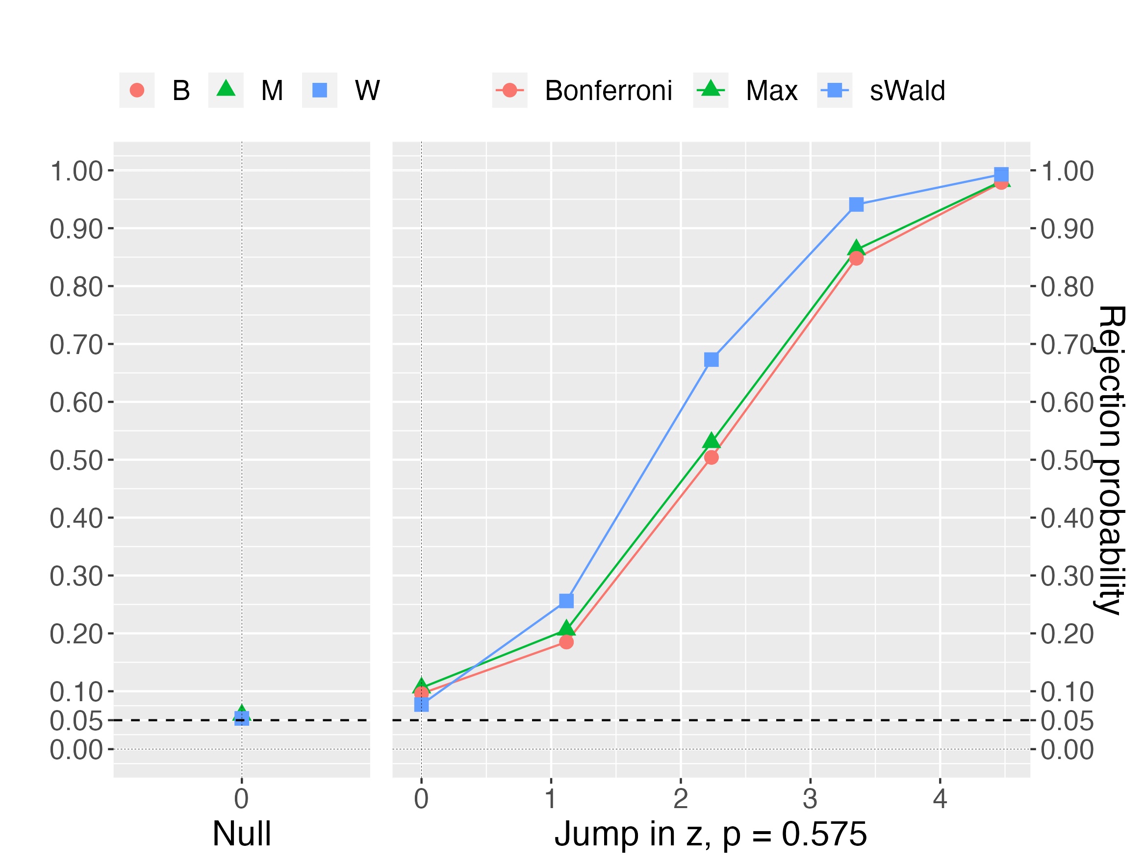
(b) Covariates have the same pairwise correlation coefficient of $0.3$

Figure 12: $1/5$ of jumps in all the five covariates with a density, $n=1000$.

(a) The remaining one has the same pairwise correlation coefficient of $0.9$.

(b) The remaining one has the pairwise correlation coefficient of $-0.9$.

Figure 13: A jump in the three covariates with a density, $n=1000$. Two out of three covariates have the same pairwise correlation coefficient of $0.9$

(a) The remaining one has the same pairwise correlation coefficient of $0.9$.

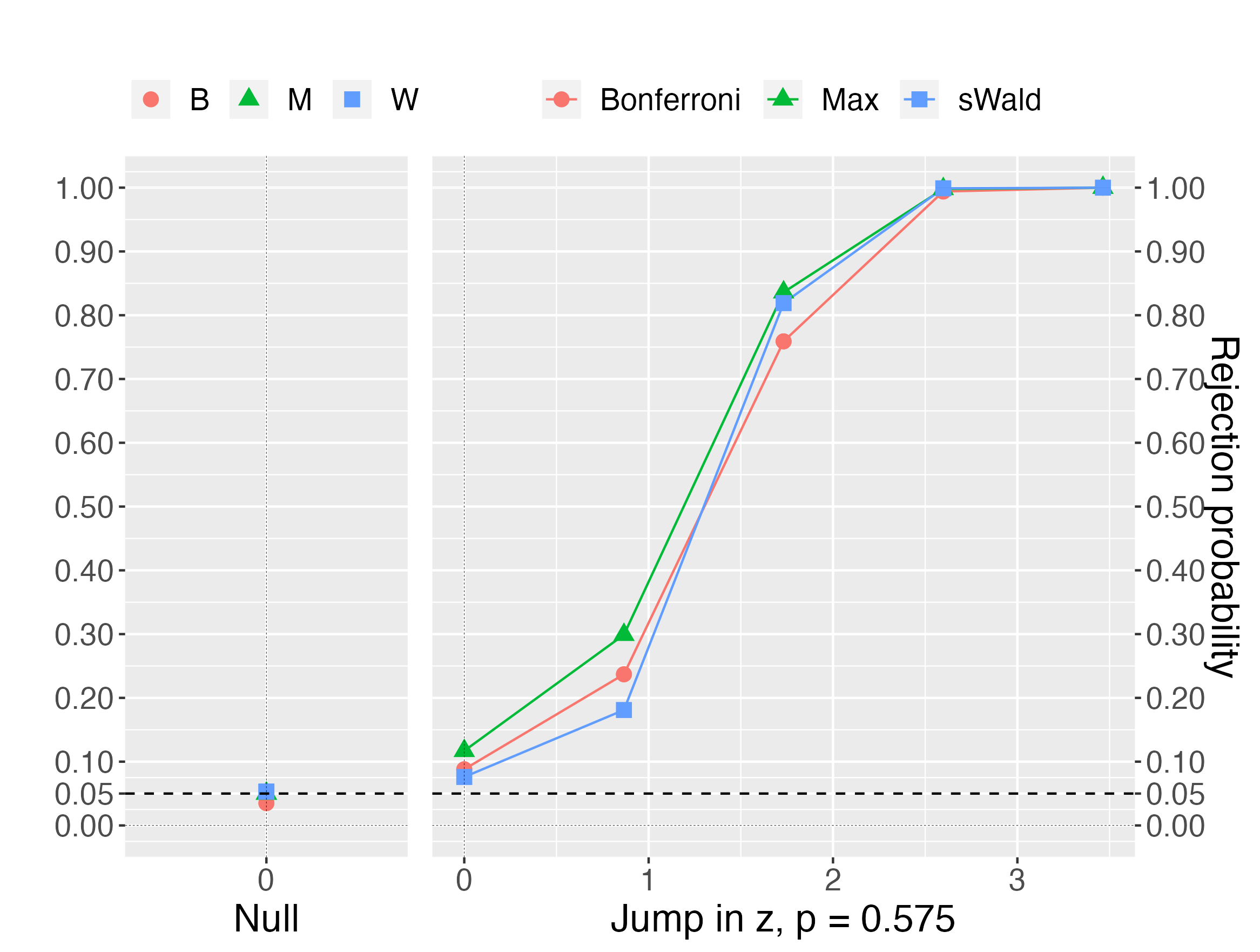
(b) The remaining one has the pairwise correlation coefficient of $-0.9$.

Figure 14: $1/3$ of jumps in all the three covariates with a density, $n=1000$. Two out of three covariates have the same pairwise correlation coefficient of $0.9$

References

- Bugni and Canay (2021) Bugni, F. A. and I. A. Canay (2021): “Testing Continuity of a Density via g-order Statistics in the Regression Discontinuity Design,” Journal of Econometrics, 221, 138–159.
- Calonico et al. (2020) Calonico, S., M. D. Cattaneo, and M. H. Farrell (2020): “Optimal bandwidth choice for robust bias-corrected inference in regression discontinuity designs,” The Econometrics Journal, 23, 192–210.
- Calonico et al. (2022) ——— (2022): “Coverage error optimal confidence intervals for local polynomial regression,” Bernoulli, 28, 2998–3022.
- Calonico et al. (2017) Calonico, S., M. D. Cattaneo, M. H. Farrell, and R. Titiunik (2017): “Rdrobust: Software for Regression-discontinuity Designs,” The Stata Journal, 17, 372–404.
- Calonico et al. (2014) Calonico, S., M. D. Cattaneo, and R. Titiunik (2014): “Robust Nonparametric Confidence Intervals for Regression-Discontinuity Designs,” Econometrica, 82, 2295–2326.
- Calonico et al. (2015) ——— (2015): “Optimal data-driven regression discontinuity plots,” Journal of the American Statistical Association, 110, 1753–1769.
- Canay and Kamat (2018) Canay, I. A. and V. Kamat (2018): “Approximate Permutation Tests and Induced Order Statistics in the Regression Discontinuity Design,” The Review of Economic Studies, 85, 1577–1608.
- Cattaneo et al. (2015) Cattaneo, M. D., B. R. Frandsen, and R. Titiunik (2015): “Randomization Inference in the Regression Discontinuity Design: An Application to Party Advantages in the U.S. Senate,” Journal of Causal Inference, 3, 1–24.
- Cattaneo et al. (2019) Cattaneo, M. D., N. Idrobo, and R. Titiunik (2019): A Practical Introduction to Regression Discontinuity Designs: Foundations, Cambridge University Press.
- Cattaneo et al. (2023) ——— (2023): “A Practical Introduction to Regression Discontinuity Designs: Extensions,” arXiv:2301.08958 [econ, stat].
- Cattaneo et al. (2018) Cattaneo, M. D., M. Jansson, and X. Ma (2018): “Manipulation testing based on density discontinuity,” The Stata Journal, 18, 234–261.
- Cattaneo et al. (2020) ——— (2020): “Simple local polynomial density estimators,” Journal of the American Statistical Association, 115, 1449–1455.
- Cattaneo et al. (2016) Cattaneo, M. D., R. Titiunik, and G. Vazquez-Bare (2016): “Inference in Regression Discontinuity Designs under Local Randomization,” The Stata Journal, 16, 331–367.
- DiNardo and Lee (2011) DiNardo, J. and D. S. Lee (2011): Chapter 5 - Program Evaluation and Research Designs In O. Ashenfelter and D. Card (Ed.). Handbook of Labor Economics, Elsevier, vol. 4, 463–536.
- Durrett (2019) Durrett, R. (2019): Probability: theory and examples, vol. 49, Cambridge university press.
- Fan and Gijbels (1996) Fan, J. and I. Gijbels (1996): Local polynomial modelling and its applications: monographs on statistics and applied probability 66, vol. 66, CRC Press.
- Fort et al. (2020) Fort, M., A. Ichino, and G. Zanella (2020): “Cognitive and Noncognitive Costs of Day Care at Age 0–2 for Children in Advantaged Families,” Journal of Political Economy, 128, 158–205.
- Imbens and Lemieux (2008) Imbens, G. W. and T. Lemieux (2008): “Regression discontinuity designs: A guide to practice,” Journal of Econometrics, 142, 615–635.
- Ishihara and Sawada (2023) Ishihara, T. and M. Sawada (2023): “Manipulation-Robust Regression Discontinuity Designs,” arXiv:2009.07551 [econ, stat].
- Korting et al. (2023) Korting, C., C. Lieberman, J. Matsudaira, Z. Pei, and Y. Shen (2023): “Visual Inference and Graphical Representation in Regression Discontinuity Designs,” The Quarterly Journal of Economics, qjad011.
- Lee (2008) Lee, D. S. (2008): “Randomized Experiments from Non-Random Selection in U.S. House Elections,” Journal of Econometrics, 142, 675–697.
- Lee and Lemieux (2010) Lee, D. S. and T. Lemieux (2010): “Regression Discontinuity Designs in Economics,” Journal of Economic Literature, 48, 281–355.
- McCrary (2008) McCrary, J. (2008): “Manipulation of the Running Variable in the Regression Discontinuity Design: A Density Test,” Journal of Econometrics, 142, 698–714.
- Otsu et al. (2013) Otsu, T., K.-L. Xu, and Y. Matsushita (2013): “Estimation and Inference of Discontinuity in Density,” Journal of Business & Economic Statistics, 31, 507–524.
- Serfling (1980) Serfling, R. J. (1980): Approximation theorems of mathematical statistics, John Wiley & Sons.
- van der Vaart and Wellner (1996) van der Vaart, A. W. and J. A. Wellner (1996): Weak convergence and empirical processes, Springer New York, NY.