Robust parameter estimation from pulsar timing data

Abstract

Recently, global pulsar timing arrays have released results from searching for a nano-Hertz gravitational wave background signal. Although there has not been any definite evidence of the presence of such a signal in residuals of pulsar timing data yet, with more and improved data in future, a statistically significant detection is expected to be made. Stochastic algorithms are used to sample a very large parameter space to infer results from data. In this paper, we attempt to rule out effects arising from the stochasticity of the sampler in the inference process. We compare different configurations of nested samplers and the more commonly used markov chain monte carlo method to sample the pulsar timing array parameter space and account for times taken by the different samplers on same data. Although we obtain consistent results on parameters from different sampling algorithms, we propose two different samplers for robustness checks on data in the future to account for cross-checks between sampling methods as well as realistic run-times.

1 Introduction

Pulsars Timing Arrays (PTAs) (Detweiler (1979); Hellings & Downs (1983)) aim to detect the stochastic Gravitational Wave Background (GWB). A GWB signal is likely created by the superposition of gravitational waves emitted by Super Massive Black Hole Binaries (SMBHBs) (Rosado et al. (2015)), but there could be other sources like a relic from inflation (Grishchuk (2005)) or cosmic strings (Vilenkin (1981); Vilenkin & Shellard (2000)). While increasingly constraining upper limits have been placed on the amplitude of the GWB there has been no detection of this signature yet. However all operational PTAs are currently detecting a common but spatially uncorrelated red noise process (Ferdman et al. (2010); Manchester et al. (2013); Hobbs et al. (2010); Jenet et al. (2009)). This might indicate that the GWB signal will be detected with statistical significance in the near future. In this paper, we look at consistencies between a variety of stochastic samplers used to sample a large parameter space, where the latter is of paramount importance to inferring properties of the GWB signal.

The size of pulsar timing models necessitates the use of a hybrid frequentist and Bayesian analysis, where the pulsar timing model parameters are first obtained using iterative least square fitting with tools such as TEMPO2 (Hobbs et al. (2006); Edwards et al. (2006); Hobbs et al. (2009)) or PINT (Luo et al. (2021)) to obtain a set of timing residuals. These timing residuals are then modelled to remove excess delays due to red noise processes as well as fluctuations from the variations in the ionised interstellar medium codified as dispersion-measure models using Bayesian analysis, while analytically marginalising over the timing model parameters. This is typically called single pulsar noise analysis (SPNA). Even with this simplification, the estimation of the red noise and dispersion-measure model parameters remains computationally expensive. Further, in the final stage, when searching for the GWB, all pulsar models must be simultaneously fitted for, along with a model for the correlated signal from the GWB as well as any other correlated or uncorrelated common noise processes. Even when the search is optimised for the smallest number of pulsars, this can lead to final dimensions of the order of hundreds of parameters. Further, for the individual pulsar models as well as the final GWB search, it is desirable to carry out model selection (Jeffreys (1998); Raftery (1996)) – a method which is particularly well suited for Bayesian analysis.

This mixed approach implies inherent uncertainties in the comparision of the algorithms themselves as well as any difference in the obtained results. We attempt to address this issue by adapting the most commonly used PTA analysis package, enterprise, to utlise a number of nested sampling algorithms. We perform single pulsar noise analyses for a set of six pulsars, first utlised for the recent limits presented by the European Pulsar timing Array (EPTA) (Chen et al. (2021)). Using the most performant nested sampling algorithm as determined from the SPNA analysis, we then search for the GWB using both the pulsar dataset as well as the second International Pulsar Timing Array (IPTA) second mock data challenge (MDC) (Hazboun et al. (2018)).

In Sec. 2, we briefly summarise the data we have used for our inference process. Section 3 serves as an introduction to Bayesian inference with focus on noise models used in this paper and pulsar timing data in general. Some technical details to algorithms we use are also included. We give a summary of our results in Sec. 4 and conclude in Sec. 5.

2 Data

We have used data recently utilised by the EPTA collaboration (Chen et al. (2021)), and focussed on six pulsars – PSRs J0613-0200, J1012+5307, J1600-3053, J1713+0747, J1744-1134 and J1909-3744. The times of arrival (TOAs) of these pulsars are fitted using the TEMPO2 software to pulsar timing models describing the pulsars astrometric, intrinsic and environmental properties, along with simple polynomial models for the variations of ionised interstellar medium (IISM) along the line of sight to these pulsars. The resulting ‘timing residuals’ are shown in Fig. 1 where we highlight the large number of observing systems used for each pulsar dataset by different colours. We refer the interested reader to (Chen et al. (2021)) and forthcoming EPTA publications for more details on the individual observing systems but list the names here. the abbreviations correspond to the Pulsar Machine (P1, P2 and PuMaI/II) instruments at the Westerbork Synthesis Radio Telescope (WSRT), the Reconfigurable Open Architecture Computing Hardware (ROACH) and the Digital Filter Bank (DFB) based devices at the Jodrell Bank Observatory (JBO), the Berkeley-Orleans-Nançay (BON) and the Nancay Ultimate Pulsar Processign Instrument (NUPPI) at the Nançay Radio Observatory, and the PSRIX instrument (labelled P217, P200, S110 and asterix) at the Effelsberg radio telescope. The residuals of Fig. 1 encode within them the signatures of contributions from pulsar specific low and high frequency processes as well as common astrophysical signals, such as perturbations due to Solar system bodies (Champion et al. (2010); Caballero et al. (2018)), time-variable delays due to density fluctuations in the IISM along the line of sight to the pulsar or the spatially-correlated GWB.

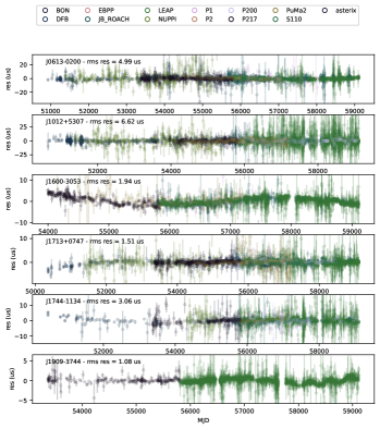
Figure 1: Timing residuals for the 6 pulsars from Chen et al. (2021). Colors denote the different data recording systems (or backends) used and the labels are described in the text.

In addition to real data, to test different samplers, we have also used simulated timing data, generated by the IPTA collaboration (Verbiest et al. (2016)) and used in the second MDC (Hazboun et al. (2018)). From the MDC, we choose a dataset containing a GWB signal. The dataset consists of 33 pulsars, and in addition to the GWB, each individual pulsar is characterised by its own spin noise or red noise. The data also contains white noise characterising the observing telescopes. The simulated dataset spans a timeline of 15 years, and is observed at a central frequency of 1440 MHz. The times of arrival (TOAs) are uniformly distributed with obsevations taken every 30 days.

The extraction of the GWB signal is a complicated process due to the need to transform radio pulsar observations into reference times at which a group of photons from each pulsar in the PTA arrive at Earth or Solar System Barycentre. While the observed data are the TOAs, the data analysis is done on timing residuals. For this the TOAs are first converted into residuals, obtained after subtracting the predicted timing model from the observed TOAs. If the predicted model fits the observations perfectly, the residuals will be identically 0. In addition to the presence of a GWB, additional non-gravitational-wave related noise sources may alter the TOAs, some of these noise models are described in Sec. 3.

3 Bayesian analysis and parameter estimation setup

We perform Bayesian inference on the pulsar timing data and sample over parameters corresponding to noise models describing the variations in the residuals as described below. We sample over single pulsars (henceforth, SPNA analysis) as well as the full pulsar timing array (henceforth, PTA analysis) and use different samplers to test the consistency of the inferred noise models. Although nested sampling would appear to be naturally desirable for PTA analysis, analyses such as those from the Parkes PTA (PPTA) or NANOGRAV typically utilise the Parallel Tempering Markov Chain Monte Carlo (PTMCMC) (Ellis & van Haasteren (2017)) method due to the lower computational cost. Since PTMCMC does provide direct access to the marginal likelihoods, methods such as the Savage-Dickey approximation and hypermodel sampling are employed for model comparison. Even though the EPTA and IPTA results have been presented in the literature which utilise efficient multi-ellipsoidal nested sampling algorithms such as MultiNest and Polychord for SPNA, the final search for the GWB still utilises PTMCMC or similar Markov Chain Monte Carlo (MCMC) based methods.

3.1 Bayesian inference

We provide a very brief summary of Bayesian inference to make our study self-contained. We point the reader to detailed resources like (Sivia & Skilling (2006); Gregory (2005)) for further reading. Bayesian analysis estimates parameters from probability distribution functions (PDFs). The posterior PDF is obtained by providing the initial prior PDF and using that in combination with the likelihood, containing information about the data. The Bayes’ theorem can be written down as

$$P(\vec{\theta}|d)=\frac{P(d|\vec{\theta})P(\theta)}{P(d)}.$$ (1)

where $\vec{\theta}$ refers to a multidimensional parameter set, $d$ is the data and the notation $P(\vec{\theta}|d)$ refers to information on $\theta$ given $d$. Deatils of the likelihood calculation in case of analysis of pulsar timing data may be found in (Arzoumanian et al. (2015)) and references therein. In addition to estimating parameters by using prior knowledge as well as knowledge from observed data, Bayesian analysis allows us to perform model selection. With the data remaining the same, this means performing an analysis each time with a different model. In that case, Eqn. 1 may be rewritten as

$$P(\mathcal{H}|d)=\frac{P(d|\mathcal{H})P(\mathcal{H})}{P(d)}.$$ (2)

$\mathcal{H}$ represents a hypothesis and in case of pulsar analysis, $\mathcal{H}$ may be assuming that the timing data contains a GWB signal, $\mathcal{H}_{\mathrm{GWB}}$ or only a common red noise signal (CRN), $\mathcal{H}_{\mathrm{CRN}}$ but not a GWB. From Eqn. 2, if we then compute the ratio of probabilities $P(\mathcal{H}_{\mathrm{GWB}})$ and $P(\mathcal{H}_{\mathrm{CRN}})$ we get a quantitative measure of which model is more preferred by the data.

3.2 Noise models

When analysing single pulsar data, we focus only on individual pulsars’ intrinsic red noise (RN), the noise from disperson measure arising from the interstellar medium (DM), and white noise (WN), inherent to the observing telescopes. In addition, when sampling over the parameter space of a PTA analysis, we include a CRN. When the common process includes spatial correlations, we search for a common GWB. We briefly describe each of the noise processes below:

3.2.1 White Noise

The white noise itself can be divided into two parts: (i) a multiplicative factor of the estimated error bar on the observed TOAs, the $\mathrm{EFAC}$ and (ii) an additional noise adding in quadrature to the error bars, the $\mathrm{EQUAD}$. Both these components vary across the different observing telescopes even if they all observe the same pulsar. The total error on a TOA, $\sigma$ can be written as

$$\sigma=\sqrt{(\sigma\mathrm{EFAC})^{2}+\mathrm{EQUAD}^{2}}.$$ (3)

$\mathrm{EFAC}$ represents possible uncertainty on the TOA error estimation during the cross-correlation of the pulsar profile with the stndard template (Taylor (1992)), and $\mathrm{EFAC}$ may arise from physical effects like pulsar jitter noise and give rise to additional scatter of the TOAs (EKERS & MOFFET (1968)).

3.2.2 Red Noise

Red noise is intrinsic to each pulsar, and also commonly referred to as spin-noise. This arises primarily as a result of irregularilities in pulsar-spin (Cordes & Downs (1985); D’Alessandro et al. (1995)). The imprint on the pulsar residuals from the intrinsic noise is also a red process, like the GWB, and the power spectrum may be described as a powerlaw

$$\phi_{\mathrm{RN}}=\frac{A_{\mathrm{RN}}^{2}}{12\pi^{2}}\left(\frac{1}{1\ \mathrm{yr}}\right)^{-3}\frac{f^{-\gamma_{\mathrm{RN}}}}{T},$$ (4)

where $A_{\mathrm{RN}}$ and $\gamma_{\mathrm{RN}}$ are the amplitude and spectral index of the red noise process respectively, and $T$ is the total timespan between latest and earliest TOA.

3.2.3 Dispersion Measure Noise

As the pulses from a pulsar travel through the interstellar medium, the imprint of the interstellar medium is also encoded on the TOAs. Dispersion measure is time-varying and defined as the integrated column density of free electrons in the pulsar’s line of sight (You et al. (2007)). Unlike intrinsisc red noise, this noise is frequency-dependent and follows a $\nu^{-2}$ dependence, $\nu$ being the radio frequency. This source maybe further described by an additional powerlaw spectrum of the form

$$\phi_{\mathrm{DM}}=A_{\mathrm{DM}}^{2}\left(\frac{1}{1\ \mathrm{yr}}\right)^{-3}\frac{f^{-\gamma_{\mathrm{DM}}}}{T}\left(\frac{1400\ \mathrm{MHz}}{\nu}\right)^{2},$$ (5)

where $A_{\mathrm{DM}}$ and $\gamma_{\mathrm{DM}}$ are the amplitude and spectral index of the dispersion noise respectively.

3.3 Samplers

As described above, the parameter space of even a single pulsar is multidimensional and we use techniques of stochastic sampling to infer the noise properties of pulsars. To compare among different samplers, we use nested sampling (Skilling (2006)) as well as MCMC methods, where the latter is also conventionally used in inference from pulsar timing data (Ellis & van Haasteren (2017)). We have made use of the modular nature of the analysis code Enterprise and incorporated different nested samplers to be used with the Likelihood function available within the code. We also use the native PTMCMC sampler, both with and without message-passing-interface (MPI) (Message Passing Interface Forum (2021)), making a thorough study of performances from different kinds of samplers. We briefly describe the individual samplers used in this paper below.

3.3.1 PTMCMC

Markov Chain Monte Carlo (MCMC) (Raftery (1996); Gamerman & Lopes (2006)) is one of the commonest methods to stochastically sample a parameter space. Furthermore, Parallel Tempering (Swendsen & Wang (1986); Geyer (1991)) is incorporated to explore the parameter space at different temperatures, thereby enabling a denser sampling. PTMCMC is natively used in the pulsar timing software Enterprise. MCMC directly samples the posterior distribution and after the intial stage, called burn-in, gathers samples which are the representative posterior samples. In this paper, we have used in addition to PTMCMC, also its MPI-enabled version (henceforth, PTMCMC-MPI) and we notice a speedup of around a factor of two in most cases.

3.3.2 PyMultiNest

Conventionally, the nested sampling method samples the prior by distributing live points and exploring the parameter space by finding higher regions of likelihood. Each live point forms a contour on the likelihood surface which gets updated as live points corresponding to lower likelihood values get replaced by ones associated with higher likelihood values. Ref. Feroz et al. (2009) updated this method by forming regions on the likelihood surface and associating them to multiple multidimensional ellipsoids. Furthermore, this has been made more user-friendly by introducing a Python interface in Buchner et al. (2014) called PyMultinest. In this paper, we use the parallelised version of the same by interfacing it with the MPI protocol.

3.3.3 Dynesty

The nested sampling method described above is known as Static Nested Sampling. In addition, the Dynesty sampler (Speagle (2020)) also includes Dynamic Nested Sampling. Throughout our paper, we have however used the Static sampler from within Dynesty. The configuration we have when using Dynesty relies on constructing the ellipsoids as implemented in MultiNest and as such differs only in the use of the paralleslisation through MPI as we now parallelise sampling the prior. In addition, the decision of when to contruct multiple bounds differs in Dynesty as opposed to MultiNest. Further information may be found also in dyn . Our implementation follows the call to Dynesty as in Smith et al. (2020) and we have adopted the approach of parallelisation as in the pubicly available pBilby code.

3.3.4 UltraNest

UltraNest (Buchner (2021)) is a newly introduced nested sampling algorithm. It is designed to ensure accurate sampling of the parameter space, especially in the cases of widely separated minima or tightly correlated parameter density distribution for which multi-ellipsoidal algorithms such as MultiNest have been shown to fail. UltraNest utlises the Radfriends (Buchner (2016)) algorithm along with flexible penalisation schemes which are dynamically reconfigured to allow resampling of previously sampled regions. We have utilised the Reactive nested sampling algorithm of UltraNest for our test, as we found no discernible benefits from using the static version in our initial testing. It should be noted that the hybrid frequentist and Bayesian approach of standard PTA analysis means this article presents a restrictive comparision for UltraNest as this algorithm is expected to perform better with very large numbers of model parameters.

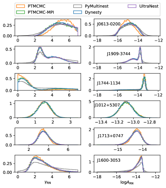
Figure 2: Posterior PDFs across different samplers representing inferred red noise models from SPNA on each of the 6 pulsars from EPTA-DR2. We do not show the results from PyMultiNest on J1713+0747 and J1012+5307 and UltraNest results on J1744-1134 and J1012+5307. These did not finish after several months.

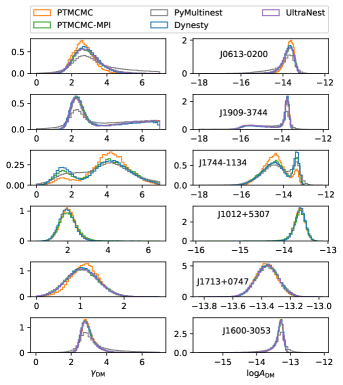
Figure 3: Posterior PDFs across different samplers representing inferred dispersion measure noise models from SPNA on each of the 6 pulsars from EPTA-DR2. We do not show the results from PyMultiNest on J1713+0747 and J1012+5307 and UltraNest results on J1744-1134 and J1012+5307. These did not finish after several months.

4 Results

We present the results from the SPNA analyses on the 6 pulsars from the EPTA and present results from the full PTA analyses from the simulated dataset. For the SPNA analyses, we have recorded the time taken by each sampler. For the PTA analysis, we focus only on the fastest of the nested samplers and use PTMCMC for comparison between two types of samplers. The intrinsic parameters being sampled over and their respective prior ranges are given in Tab. 1.

Parameter	Prior range
$\log{A_{\mathrm{RN}}}$	[-18, -10]
$\gamma_{\mathrm{RN}}$	[0,7]
$\log{A_{\mathrm{DM}}}$	[-18, -10]
$\gamma_{\mathrm{DM}}$	[0,7]
$\log{A_{\mathrm{GWB}}}$	[-18, -10]
$\gamma_{\mathrm{GWB}}$	[0,7]

Table 1: Prior ranges used; for SPNA runs, the $\mathrm{RN}$ and $\mathrm{DM}$ related parameters are being varied for each pulsar whereas the additional $\mathrm{GWB}$-related parameters are varied in case of the PTA analysis.

4.1 SPNA

We present results only on RN and DM as these directly affect the TOAs and are intrinsic to the pulsars. Fig. 2 shows the amplitude and spectral index of the RN noise models inferred from the respective 6 EPTA pulsars. The models are presented in the form of posterior Probability Density Functions (PDFs). Fig. 3 shows the same for the DM noise models. In each case, we show results obtained from different samplers; we show results from PTMCMC, PTMCMC-MPI, PyMultiNest, Dynesty and UltraNest. In case of the nested samplers, we have used 4096 live points and have used $2\times 10^{6}$ posterior samples for the PTMCMC-based runs for each pulsar. Since we have used the samplers each time in combination with the generic package Enterprise the likelihood model therefore remains the same and the results show the robustness of the sampling as the PDFs are very consistent with each other. We quantify the differences in PDFs by giving the values of Kolmogorov-Smirnov (KS) statistic (Kolmogorov (1933); Smirnov (1948)) in Table. 2. If the cumulative distributions corresponding to two posterior distributions $p_{1}(x)$ and $p_{2}(x)$ are $P_{1}(x)$ and $P_{2}(x)$ respectively, the KS statistic is the largest difference:

$$\mbox{KS}=\mbox{sup}_{x}|P_{1}(x)-P_{2}(x)|.$$ (6)

From the above definition, the KS value always lies between 0 and 1. If we find the values to be closer to 0, we may consider the underlying PDFs $p_{1}(x)$ and $p_{2}(x)$ to be very close to each other. A source of differences in PDFs is however the stochasticity of the algorithm itself; this is in addition to inherent differences between the PDFs being compared. To quantify for this and establish a threshold from the stochasticity itself, for each parameter of each pulsar and for each sampler, we generated 20 sets of resampled posterior samples and computed the KS statistic values between all combinations of these 20 data sets. The maximum KS statistic arising from this study for all parameters and sampler for each pulsar is always $\sim 10^{-3}$, the highest values overall being for J1744-1134, and the $\log{A_{\mathrm{DM}}}$ parameter, $\sim 0.007$. So, from Tab. 2, we take values $>10^{-3}$ to signify a difference in the PDF arising inherently. From Tab. 2, the highest KS value is $\sim$ 0.3 between PTMCMC and PyMultiNest for J0613-0200 as well as J1744-1134. We can conclude that from these values, the PDFs among different samplers are indeed quite close to each other as is also visually noted from Fig. 2 and Fig. 3. This leads us to conclude that the parameter estimates obtained from the data are indeed indicative of a physical process and not an artifact of sampling. We notice PTMCMC combined with MPI gives a speedup in all cases, and while that is a significant gain in runtimes, we note that the algorithm, when coupled with MPI, is different from the native PTMCMC. PTMCMC, when used in a single core, does not do parallel tempering (the name is a misnomer in this case). It is only when coupled with MPI, that there is a single temperature per thread and the parallel tempering kicks in Moreover, from Figs. 2 and 3, we note that PTMCMC-MPI results are closer to those obtained with parallel nested samplers. This is likely because the multiple chains running with different temperatures in case of PTMCMC-MPI, allow a more exhaustive exploration of the parameter space, making the final posterior PDFs closer to those obtained using nested samplers. We also note that, among nested samplers, UltraNest and Dynesty show excellent agreement, whereas PyMultiNest distributions tend to be slightly different. While all the nested samplers that we have used in this work rely on the underlying algorithm MultiNest, there are subtle differences among PyMultiNest, Dynesty and UltraNest. UltraNest and Dynesty have slight improvements over MultiNest (and therefore PyMultiNest) and our results suggest that MultiNest in itself is probably not good enough to sample the complex and high dimensional parameter space of the pulsars except in the simplest cases. It may be worth trying to do PyMultiNest analyses with finer settings, however that would not be a one-to-one comparison amongst samplers as is our goal here. In this analysis, we have only changed the sampler. A robust check of the likelihood function would be to keep the sampler the same and change the likelihood definition. The existing software TempoNest (Lentati et al. (2014)) is independent of Enterprise and defines the likelihood function independently. It inherently uses the MultiNest sampler, a check of the likelihood function may be to repeat an analysis with TempoNest and Enterprise coupled with PyMultiNest. This will be studied in a future publication. Finally, in Tab. 3 we note the walltime in hours taken by each sampler on the same data. We also note the number of dimensions, $\mathrm{N_{dim}}$, and number of TOAs, $\mathrm{N_{TOAs}}$ for each pulsar. We have used the same machine for all SPNA runs to have a fair comparison of walltimes. A reason for Dynesty’s speedup is also the parllelisation of the prior-sampling, as mentioned in Smith et al. (2020). Specifically, for the pulsars J1713+0747 and J1012+5307, we were unable to get the sampler to converge after these runs took at least 80 days and we do not present their results. From Tab. 3, we note that PyMultiNest becomes unusable for most pulsars; while this is mostly likely due to the increased dimensionality; indeed the missing pulsars for PyMultiNest have $\mathrm{N_{dim}}=56$ and $\mathrm{N_{dim}}=58$, this is likely also a combination of the high $\mathrm{N_{dim}}$ and the large $\mathrm{N_{TOAs}}$. In Fig. 2 and Fig. 3, all nested samplers and PTMCMC-MPI were run in parallel in one compute node using 47 sockets, where each compute node has the specification of Intel(R) Xeon(R) Gold 6252N CPU @ 2.30GHz 35.75 MB with 192GB memory and 48 sockets in total. PTMCMC in itself was run using a single socket in a compute node.

		PTMCMC vs. PTMCMC-MPI		PTMCMC vs. PyMultiNest		PTMCMC vs. Dynesty		PTMCMC vs. UltraNest
Pulsar	Parameter	Red Noise	DM Noise	Red Noise	DM Noise	Red Noise	DM Noise	Red Noise	DM Noise
$\mathrm{J0613-0200}$	$\gamma$	0.154	0.141	0.172	0.291	0.119	0.13	0.132	0.145
	$\log{\mathrm{A}}$	0.151	0.137	0.173	0.291	0.116	0.127	0.129	0.137
$\mathrm{J1909-3744}$	$\gamma$	0.01	0.009	0.094	0.117	0.023	0.041	0.012	0.016
	$\log{\mathrm{A}}$	0.009	0.006	0.074	0.120	0.020	0.043	0.012	0.018
$\mathrm{J1600-3053}$	$\gamma$	0.079	0.038	0.196	0.185	0.062	0.035	0.086	0.037
	$\log{\mathrm{A}}$	0.074	0.03	0.251	0.119	0.055	0.017	0.08	0.026
$\mathrm{J1012+5307}$	$\gamma$	0.042	0.042	-	-	0.042	0.050	-	-
	$\log{\mathrm{A}}$	0.017	0.037	-	-	0.034	0.042	-	-
$\mathrm{J1713+0747}$	$\gamma$	0.073	0.095	-	-	0.062	0.077	0.072	0.088
	$\log{\mathrm{A}}$	0.073	0.057	-	-	0.064	0.036	0.072	0.049
$\mathrm{J1744-1134}$	$\gamma$	0.129	0.114	0.291	0.153	0.154	0.154	-	-
	$\log{\mathrm{A}}$	0.113	0.112	0.295	0.166	0.136	0.150	-	-

Table 2: Results on KS statistics on 6 pulsars from SPNA results from different samplers. The runs which ended up being unfinished after months do not have KS statistics’ values associated with them and are given as ’-’. The values are shown differently for the red noise and dispersion measure models, and for the two parameters, the amplitude and spectral index separately.

Pulsar			Sampler
Name	$\mathrm{N_{dim}}$	$\mathrm{N_{TOAs}}$	PTMCMC	PTMCMC-MPI	PyMultiNest	Dynesty	UltraNest
$\mathrm{J0613-0200}$	50	3022	9.91	8.82	745.69	6.83	42.25
$\mathrm{J1909-3744}$	18	2817	13.61	5.60	3.40	1.68	2.11
$\mathrm{J1600-3053}$	30	3345	19.06	7.16	16.27	3.5	220
$\mathrm{J1012+5307}$	56	5837	28.80	13.94	-	11.92	-
$\mathrm{J1713+0747}$	58	5052	29.11	14.82	-	15.95	141.32
$\mathrm{J1744-1134}$	38	1980	19.66	6.49	321	4.5	-

Table 3: Walltime in hours for the SPNA runs with each sampler, for each pulsar the number of dimensions and number of TOAs are also given as $\mathrm{N_{dim}}$ and $\mathrm{N_{TOAs}}$ respectively. The unfinished runs’ times are shown as ‘-’. From this table, we note that only PTMCMC and Dynesty are expected to finish within a feasible timescale. Furthermore, when used with MPI, runtimes with PTMCMC can be scaled up. For some pulsars, the speedup obtained is up to a factor of 2.

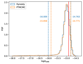
Figure 4: Posterior PDF of the log of GWB amplitude from analysing MDC2 data; the injected value is shown with the red vertical line and is $\log{A_{\mathrm{GWB}}}=-14.89$. The dashed vertical lines refer to the 5% and 95% quantiles respectively, we note the injected value always falls within this limit. The spectral index $\gamma$ is kept fixed to 4.33 and for comparison two samplers PTMCMC (orange) and Dynesty (blue) are being run, showing good agreement. For each sampler, the respective values of quantiles (shown in orange for PTMCMC and in blue for Dynesty) also lie very close to each other.

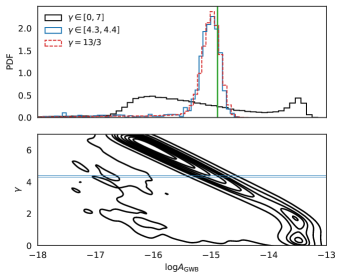
Figure 5: Comparison between varying and fixing the spectral index $\gamma$. The top panel shows the 1D posterior PDFs of the log of the GWB amplitude, $\log{A_{\mathrm{GWB}}}$. The three posteriors correspond to when the spectral index, $\gamma$ is varying in the sampling (black), when the spectral index is fixed to 13/3 in the run (dashed, red) and when the $\log{A_{\mathrm{GWB}}}$ is restricted to the indices of $\gamma$ corresponding to a narrow range of $[4.3,4.4]$ (blue) in the varying-$\gamma$ run. The injected value of $\log{A_{\mathrm{GWB}}}=-14.89$ is hown as a green vertical line. The bottom panel shows the two-dimensional plot of $\gamma$ versus $\log{A_{\mathrm{GWB}}}$ when $\gamma$ is being varied in the inference run; the $\gamma$ range of $[4.3,4.4]$ corresponding to the blue PDF in the upper panel is shown in blue horizontal lines. We show only the results from Dynesty here as Fig. 4 already shows good agreement between PTMCMC and Dynesty.

4.2 PTA

In this Section, we choose the two fastest samplers from Tab. 3. In addition to being the fastest, we also use one nested sampler (Dynesty) and one MCMC sampler (PTMCMC) for consistency checks between two different methods of sampling. Since we do an analysis on all 33 pulsars together which form the pulsar timing array in the IPTA-MDC2, we fix the WN parameters to their TEMPO2 fit values to make the analysis computationally feasible. We analyse simulated data where a GWB has been injected as mentioned in Sec. 2. The injected value of the GWB amplitude is picked up by the resulting PDFs of the GWB amplitude by both samplers as shown in Fig. 4. The figure shows the results when the analysis is done by keeping the spectral index of the GWB power spectrum fixed to 4.33. In addition, we repeated the analysis by varying both the spectral index and the GWB amplitude.This is shown in Fig. 5. The upper panel shows the results of the GWB amplitude when $\gamma$ is varied and kept fixed. In the lower panel the amplitude for the varying $\gamma$ case is plotted by choosing the amplitude values corresponding to those of $\gamma$ lying between 4.3 and 4.4 and the resulting PDF looks very similar to the case when $\gamma$ is kept fixed to 4.33.

In addition, we perform model selection between a GWB and a CRN, using both samplers. With PTMCMC, we use the hypermodel approach, available within Enterprise to extract a Bayes’ factor in favour of one of the two models. The model selection remains inconclusive from the values of Bayes’ factors obtained with either sampler. Recently Ref. Chalumeau et al. (2021) also used these two samplers to get model selection results. The values obtained from both samplers are given in Tab. 4. This shows that we are unable to assign a model to the data even when the data is ideally simulated, contains no DM noise and contains a GWB signal of considerable amplitude $A_{\mathrm{GWB}}=1.3\times 10^{-15}$. This problem of model selection will therefore become even more important in real data which will additionally contain unmodelled noise. Further, we note the uncertainties in Tab. 4 and the slightly higher uncertainty values associated with the Dynesty runs. While for hypermodel sampling, one run suffices to assign a value of Bayes’ factor to a model, with the nested sampling approach, we have to resort to separate runs for each model to get a Bayes’ factor. The error is therefore added in quadrature and adds up in the case of the runs done with Dynesty. In Sec. 5, we suggest a method to be able to assign a threshold value of Bayes’ factor to claim a detection from real data.

	$B^{\mathrm{GWB}}_{\mathrm{CRN}}$	$B^{\mathrm{Fix}\ \gamma}_{\mathrm{Vary}\ \gamma}$
Dynesty	0.534 $\pm$ 1.148	0.945 $\pm$ 1.147
PTMCMC	1.279 $\pm$ 0.018	0.955 $\pm$ 0.011

Table 4: Model selection results: Bayes’ factors between models GWB and CRN compared with samplers PTMCMC and Dynesty.

5 Conclusions

We have compared different algorithms to sample the parameter space of the pulsar likelihood. We have used samplers to infer models from six single pulsars as well as a PTA comprised of thirty three pulsars. In each case, we note good agreement between different sampling algorithms and from estimates of run-time as well as to maintain a balance between different ways of sampling, propose the use of PTMCMC and Dynesty as preferred methods for future inference from pulsar timing data.

In future we will generate data with randomized sky positions for the pulsars, commonly referred to as sky-scrambling (Taylor et al. (2017)), to resemble a realistic realisation of measured data and will construct a distribution of Bayes’ factors to build a ‘background’. Furthermore, we will inject GWB signals and infer their properties and compare the resulting Bayes’ factors distribution. This will likely give us an idea of the threshold Bayes’ factor to claim a detection of a GWB, if present in data. This work is in progress and will be published separately.

Data Availability

The paper has made use of data on 6 single pulsars, results from whose analyses have been published by the EPTA in Chen et al. (2021) and MDC data simulated by the IPTA, available in https://github.com/ipta/mdc2/.

References

- Arzoumanian et al. (2015) Arzoumanian Z., et al., 2015, Astrophys. J., 813, 65
- Buchner (2016) Buchner J., 2016, Statistics and Computing, 26, 383
- Buchner (2021) Buchner J., 2021, The Journal of Open Source Software, 6, 3001
- Buchner et al. (2014) Buchner J., et al., 2014, Astron. Astrophys., 564, A125
- Caballero et al. (2018) Caballero R. N., et al., 2018, Mon. Not. Roy. Astron. Soc., 481, 5501
- Chalumeau et al. (2021) Chalumeau A., et al., 2021, Mon. Not. Roy. Astron. Soc., 509, 5538
- Champion et al. (2010) Champion D. J., et al., 2010, Astrophys. J. Lett., 720, L201
- Chen et al. (2021) Chen S., et al., 2021, ] 10.1093/mnras/stab2833
- Cordes & Downs (1985) Cordes J. M., Downs G. S., 1985, Astrophysical Journal, Suppl., 59, 343
- D’Alessandro et al. (1995) D’Alessandro F., McCulloch P. M., Hamilton P. A., Deshpande A. A., 1995, Monthly Notices of the Royal Astronomical Society, 277, 1033
- Detweiler (1979) Detweiler S. L., 1979, Astrophys. J., 234, 1100
- EKERS & MOFFET (1968) EKERS R., MOFFET A., 1968, Nature, 220, 756–761
- Edwards et al. (2006) Edwards R. T., Hobbs G. B., Manchester R. N., 2006, Mon. Not. Roy. Astron. Soc., 372, 1549
- Ellis & van Haasteren (2017) Ellis J., van Haasteren R., 2017, jellis18/PTMCMCSampler: Official Release, doi:10.5281/zenodo.1037579, https://doi.org/10.5281/zenodo.1037579
- Ferdman et al. (2010) Ferdman R. D., et al., 2010, Class. Quant. Grav., 27, 084014
- Feroz et al. (2009) Feroz F., Hobson M. P., Bridges M., 2009, Monthly Notices of the Royal Astronomical Society, 398, 1601
- Gamerman & Lopes (2006) Gamerman D., Lopes H. F., 2006, Markov Chain Monte Carlo: Stochastic Simulation for Bayesian Inference. Chapman and Hall, London
- Geyer (1991) Geyer C. J., 1991, Markov Chain Monte Carlo Maximum Likelihood, https://hdl.handle.net/11299/58440
- Gregory (2005) Gregory P., 2005, Bayesian Logical Data Analysis for the Physical Sciences. Cambridge University Press, London
- Grishchuk (2005) Grishchuk L. P., 2005, Physics-Uspekhi, 48, 1235
- Hazboun et al. (2018) Hazboun J. S., Mingarelli C. M. F., Lee K., 2018
- Hellings & Downs (1983) Hellings R. w., Downs G. s., 1983, Astrophys. J. Lett., 265, L39
- Hobbs et al. (2006) Hobbs G., Edwards R., Manchester R., 2006, Mon. Not. Roy. Astron. Soc., 369, 655
- Hobbs et al. (2009) Hobbs G., et al., 2009, Mon. Not. Roy. Astron. Soc., 394, 1945
- Hobbs et al. (2010) Hobbs G., et al., 2010, Class. Quant. Grav., 27, 084013
- Jeffreys (1998) Jeffreys H., 1998, The Theory of Probability. Oxford University Press, London
- Jenet et al. (2009) Jenet F., et al., 2009, ] 10.48550/arXiv.0909.1058
- Kolmogorov (1933) Kolmogorov A., 1933, G. Inst. Ital. Attuari, 4, 83
- Lentati et al. (2014) Lentati L., Alexander P., Hobson M. P., Feroz F., van Haasteren R., Lee K., Shannon R. M., 2014, Mon. Not. Roy. Astron. Soc., 437, 3004
- Luo et al. (2021) Luo J., et al., 2021, Astrophys. J., 911, 45
- Manchester et al. (2013) Manchester R. N., et al., 2013, Publ. Astron. Soc. Austral., 30, 17
- Message Passing Interface Forum (2021) Message Passing Interface Forum 2021, MPI: A Message-Passing Interface Standard Version 4.0. https://www.mpi-forum.org/docs/mpi-4.0/mpi40-report.pdf
- Raftery (1996) Raftery A. E., 1996, Practical Markov Chain Monte Carlo. Chapman and Hall, London
- Rosado et al. (2015) Rosado P. A., Sesana A., Gair J., 2015, Mon. Not. Roy. Astron. Soc., 451, 2417
- Sivia & Skilling (2006) Sivia D., Skilling J., 2006, Data Analysis - A Bayesian Tutorial. Oxford University Press, London
- Skilling (2006) Skilling J., 2006, Bayesian Anal., 1, 833
- Smirnov (1948) Smirnov N., 1948, Ann. Math. Statist., 19, 279
- Smith et al. (2020) Smith R. J. E., Ashton G., Vajpeyi A., Talbot C., 2020, Mon. Not. Roy. Astron. Soc., 498, 4492
- Speagle (2020) Speagle J. S., 2020, Monthly Notices of the Royal Astronomical Society, 493, 3132
- Swendsen & Wang (1986) Swendsen R. H., Wang J.-S., 1986, Phys. Rev. Lett., 57, 2607
- Taylor (1992) Taylor J., 1992, Philosophical Transactions of the Royal Society of London. Series A: Physical and Engineering Sciences, 341, 117
- Taylor et al. (2017) Taylor S. R., Lentati L., Babak S., Brem P., Gair J. R., Sesana A., Vecchio A., 2017, Phys. Rev. D, 95, 042002
- Verbiest et al. (2016) Verbiest J. P. W., et al., 2016, Mon. Not. Roy. Astron. Soc., 458, 1267
- Vilenkin (1981) Vilenkin A., 1981, Physics Letters B, 107, 47
- Vilenkin & Shellard (2000) Vilenkin A., Shellard E. P. S., 2000, Cosmic Strings and Other Topological Defects. Cambridge University Press, Cambridge
- You et al. (2007) You X.-P., et al., 2007, Mon. Not. Roy. Astron. Soc., 378, 493
- (47) Dynesty Documentation, https://dynesty.readthedocs.io/en/latest/faq.html#bounding-questions