On a wider class of prior distributions for
graphical models

Abstract

Gaussian graphical models are useful tools for conditional independence structure inference of multivariate random variables. Unfortunately, Bayesian inference of latent graph structures is challenging due to exponential growth of $\mathcal{G}_{n}$, the set of all graphs in $n$ vertices. One approach that has been proposed to tackle this problem is to limit search to subsets of $\mathcal{G}_{n}$. In this paper, we study subsets that are vector subspaces with the cycle space $\mathcal{C}_{n}$ as main example. We propose a novel prior on $\mathcal{C}_{n}$ based on linear combinations of cycle basis elements and present its theoretical properties. Using this prior, we implement a Markov chain Monte Carlo algorithm, and show that (i) posterior edge inclusion estimates computed with our technique are comparable to estimates from the standard technique despite searching a smaller graph space, and (ii) the vector space perspective enables straightforward implementation of MCMC algorithms.

NATARAJAN ET AL. [supp:][nocite]supplementary_xr

[University of Oxford]Abhinav Natarajan

[National University of Singapore]Willem van den Boom

[National University of Singapore]Kristoforus Bryant Odang

[National University of Singapore; Singapore Institute for Clinical Sciences, A*STAR; University College London]Maria de Iorio

Mathematical Institute, University of Oxford, Wellington Square, Oxford OX1 2JD, United Kingdom. Email address: natarajan@maths.ox.ac.uk

Yong Loo Lin School of Medicine, National University of Singapore, 10 Medical Dr, Singapore 117597. Email address: vandenboom@nus.edu.sg

Yong Loo Lin School of Medicine, National University of Singapore, 10 Medical Dr, Singapore 117597. Email address: kristoforusbryant@u.yale-nus.edu.sg

Yong Loo Lin School of Medicine, National University of Singapore, 10 Medical Dr, Singapore 117597. Email address: mdi@nus.edu.sg

62H2205C80;05C90

1 Introduction

Gaussian graphical models (GGMs) [10, 20] have become a standard technique to represent the conditional independence structure of a set of random variables. Given an undirected graph $G=(V,E)$, the set of vertices $V=\{1,\ldots,n\}$ represents the random variables while the set of edges $E\subseteq\{(i,j)\in V\times V:i<j\}$ represents conditional dependencies between the variables. In the Bayesian literature, a latent graph $G$ is often inferred by first specifying a prior $p(G)$ on the space of graphs followed by a prior on the precision matrix $K$ conditional on the graph, $p(K\mid G)$. Then, posterior inference is performed through sampling algorithms such as Markov chain Monte Carlo (MCMC) [e.g. 15, 18] or sequential Monte Carlo (SMC) [34, 36]. One of the main challenges in graph inference is that the number of graphs grows exponentially with the number of vertices since the size of the space $\mathcal{G}_{n}$ of all graphs with $n$ vertices is $2^{n(n-1)/2}$.

There are two main lines of research addressing the computational difficulties associated with the size of graph space: (i) devising efficient sampling algorithms and (ii) considering particular subsets of $\mathcal{G}_{n}$ with desirable properties. This work explores novel subsets in light of this second direction. A particularly popular restriction of $\mathcal{G}_{n}$ consists of focusing on the set of decomposable graphs as it allows for exact posterior computation under the conjugate Hyper-Inverse Wishart prior (see, for example, [14, 15, 16, 20, 31, 39]). However, the decomposability assumption is often restrictive in applications: suppose that the “true” graph is non-decomposable. Niu et al. [26] prove that, as the number of observations goes to infinity, the posterior distribution concentrates at the minimal triangulations of the true graph. These triangulations can present $O(n\log n)$ spurious edges [8].

As an alternative to decomposable graphs, recent research effort has been devoted to consider the set of spanning trees $\mathcal{T}_{n}$ on the complete graph (i.e. the graph containing all possible edges), which is necessarily a subset of decomposable graphs as trees do not contain cycles. Højsgaard et al. [17] propose a maximum a posteriori estimator of the latent spanning tree based on Kruskal’s [19] algorithm. Schwaller et al. [30] are able to derive the exact posterior distribution of each tree in $\mathcal{T}_{n}$ given a set of observations by applying Kirchoff’s matrix tree theorem [7] while Duan and Dunson [13] propose a Bayesian model for spanning trees where the likelihood function is built on a generative graph process and leads to an efficient Gibbs sampling algorithm. Although spanning trees provide computational advantages compared to considering all graphs, they only allow inference of the “backbone” of the graph [13], i.e. the minimum spanning tree of the data generating graph, at the cost of losing information about its global structures.

In this paper, we investigate larger subsets of $\mathcal{G}_{n}$ arising from an algebraic perspective on graphs with the cycle space as the main concrete example. Firstly, note that the set $\mathcal{G}_{n}$ together with the edgewise modulo two addition $\oplus$ and the trivial multiplication (both operations are defined in Section 2.3) forms a vector space on the finite field $\mathbb{Z}_{2}$, where the set of all edges in the complete graph forms the standard basis of $\mathcal{G}_{n}$. Definitions and preliminary results about the graph vector space are deferred to Section 2.

Our work builds on the fact that alternative bases for $\mathcal{G}_{n}$ exist. In particular, we consider the example of the space spanned by linear combinations of cycles on $V$ which forms the cycle space $\mathcal{C}_{n}$. The cycle space is a proper subspace of $\mathcal{G}_{n}$ which can be spanned using bases consisting of cycles [38]. We investigate the theoretical properties of this space and of the prior distribution on graphs when the prior is specified through a prior on cycles, instead of the common practice of specifying a prior on the edges, as well as the implications for statistical inference of such a prior. We show that the cycle space $\mathcal{C}_{n}$ is a substantially smaller set than $\mathcal{G}_{n}$, though this does not notably affect posterior inference such as edge inclusion probabilities in the concluding application.

The paper is structured as follows. Section 2 reviews graphical modelling concepts, how $\mathcal{G}_{n}$ constitutes a vector space, cycle basis theory and compares the cycle space with the set of decomposable graphs. Section 3 analyses the cycle basis prior. Section 4 contains simulation studies. In Section 5, we apply the proposed algorithm to gene expression data. Section 6 concludes the paper and discusses potential future directions. All proofs can be found in Supplementary Material.

2 Background

2.1 Graph preliminaries

We consider undirected graphs with no loops and no multi-edges, also called simple graphs. A path $\gamma_{\alpha,\beta}$ between two vertices $\alpha,\beta\in V$ is a sequence of edges $(e_{1},\dots,e_{m})$ such that $v_{1}=\alpha$, $v_{m+1}=\beta$ and $e_{i}=(v_{i},v_{i+1})$ for all $i\in\{1,\dots m\}$ where every vertex in the vertex sequence $(v_{1},\dots,v_{m+1})$ is distinct. A circuit is a sequence of edges $(e_{1},\dots,e_{m})$ where $v_{1}=v_{m+1}$. A cycle is a circuit where every vertex in $(v_{1},\dots,v_{m})$ is distinct. A graph is connected when a path $\gamma_{\alpha,\beta}$ exists for all $\alpha,\beta\in V$. A graph is complete if it contains all possible edges, that is $E=\{(i,j)\in V\times V:i<j\}$. A tree is a graph where there is exactly one path between any pair of vertices. A spanning tree of a connected graph $G=(V,E)$ is a tree with vertex set $V$ and an edge set which is a subset of $E$. A star tree $T$ on the vertices $\{v_{0},\ldots,v_{n-1}\}$ is the spanning tree whose edges are $(v_{0},v_{i})$ for $i=1,\ldots,n-1$. In this case, $v_{0}$ is the root of $T$. The degree of a vertex $v$ is the number of edges incident to $v$.

2.2 Bayesian inference of GGMs

In a GGM, a graph $G=(V,E)$ on $n$ vertices models the zeros in the precision matrix $K$ of the Gaussian distribution $N(0,K^{-1})$ on the independent rows of the $N\times n$ data matrix $X$:

$$p(X\mid K)\propto|K|^{N/2}\exp(-\langle K,U\rangle/2)$$ (1)

where $U=X^{T}X$ and $\langle A,B\rangle=\mathrm{tr}(A^{T}B)$. Specifically, $K_{ij}=0$ if $(i,j)\notin E$. For Bayesian inference, Dawid and Lauritzen [9] introduce the Hyper-Inverse Wishart prior which is a conjugate prior $p(K\mid G)$ for decomposable graphs $G$. Giudici [14] and Roverato [28] generalise this idea to non-decomposable graphs, proposing the $G$-Wishart distribution $W_{G}(\delta,D)$ with degrees of freedom $\delta>2$ and rate matrix $D$ which has density

$$p(K\mid G)=\frac{1}{I_{G}(\delta,D)}|K|^{(\delta-2)/2}\exp(-\langle K,D\rangle/2)$$ (2)

with respect to the Lebesgue measure on the set of positive definite matrices with zeros imposed by $G$. Here, $I_{G}(\delta,D)$ is a normalising constant.

Combining the prior in (2) and the likelihood (1), $K\mid G,X\sim W_{G}(\delta+N,D+U)$ due to conjugacy. The likelihood for $G$ with $K$ marginalised out follows as [e.g. 3]

$$p(X\mid G)=\frac{I_{G}(\delta+N,D+U)}{(2\pi)^{Nn/2}I_{G}(\delta,D)}$$ (3)

Unfortunately, computing $I_{G}(\delta,D)$ for a general graph $G$, despite a recently derived recursive expression [35], is intractable. Monte Carlo [3] and Laplace [21] approximations have thus been suggested, along with methods that avoid the normalising constant computation entirely [40] using the exchange algorithm of Murray et al. [25]. Notably, $I_{G}(\delta,D)$ is computationally tractable for decomposable $G$, motivating the common restriction of the space of graphs $\mathcal{G}_{n}$ to decomposable graphs.

Having the marginal likelihood of the observations given a general graph, Bayesian inference is performed by defining a prior $p(G)$ on $\mathcal{G}_{n}$. Such prior distributions are usually constructed through the specification of edge inclusion probabilities. In the next section, we define a prior distribution over graph space based on more complex substructures than edges.

2.3 $\mathcal{G}_{n}$ as vector space and the cycle space

The set $\mathcal{G}_{n}$ of all graphs with $n$ vertices is part of a vector space over the finite field $\mathbb{Z}_{2}$. Here, $\mathbb{Z}_{2}$ is a field on the set $\{0,1\}$ where addition is the modulo 2 addition (i.e. $0+0=0$, $1+0=0+1=1$, and $1+1=0$) while multiplication is trivial (i.e. $0\times x=0$ and $1\times x=x$ for any $x\in\{0,1\}$). The vector space is the triple $(\mathcal{G}_{n},\oplus,\otimes)$ where $\oplus$ is the modulo 2 addition of the edges and $\otimes$ is the (trivial) multiplication such that $0\otimes G$ is the graph with no edges, and $1\otimes G=G$. Note that the set of all edges in the complete graph forms one basis of this vector space which we call the standard basis. Alternative bases exist for the same vector space, which can (i) be used as building components of a graph (in a similar way as with edges) and (ii) induce priors $p(G)$ through the specification of a distribution on the elements of the basis. For illustration, Figure 1 considers three different bases of $\mathcal{G}_{n}$ with $n=4$ vertices.

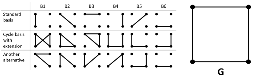
Figure 1: The table shows three different bases of the graph space $\mathcal{G}_{n}$ with $n=4$ vertices. Consider the decomposition of the graph $G\in\mathcal{G}_{n}$ on the right over each of the bases: with the standard basis, $G=\textnormal{B1}+\textnormal{B3}+\textnormal{B4}+\textnormal{B6}$. With the cycle basis, $G=\textnormal{B2}+\textnormal{B3}$. For the last basis, $G=\textnormal{B1}+\textnormal{B2}+\textnormal{B5}$.

The basis of this work is restricting the graph space in GGMs by considering subspaces of $\mathcal{G}_{n}$. A subspace of the graph vector space is a subset of $\mathcal{G}_{n}$ that is closed under $\oplus$. Restricting graphs via an appropriate subspace is desirable in GGMs for two reasons. Firstly, it shrinks the search space to a subset of $\mathcal{G}_{n}$. Secondly, being closed under addition, a subspace lends itself well to convenient Monte Carlo sampling steps as algorithms that only propose states in the subspace are readily constructed. In this paper, we focus on one particular subspace, namely the cycle space:

Definition 2.1 (Cycle space)

The cycle space $\mathcal{C}_{n}$ of graphs with $n$ vertices is the set of linear combinations of cycles in $\mathcal{G}_{n}$.

We now present some relevant properties of $\mathcal{C}_{n}$. By its definition, $\mathcal{C}_{n}$ is closed under addition making it a proper vector space:

1. The cycle space $\mathcal{C}_{n}$ is a subspace of the vector space $(\mathcal{G}_{n},\oplus,\otimes)$ [38, Theorem 5.1].

Whether a graph $G\in\mathcal{G}_{n}$ is in $\mathcal{C}_{n}$ can be conveniently checked using Veblen’s theorem:

1. A graph $G\in\mathcal{G}_{n}$ is an element of $\mathcal{C}_{n}$ if and only if every vertex has even degree in $G$, i.e. every vertex has an even number of neighbours [37].

A more intuitive description of the graphs in $\mathcal{C}_{n}$ is that they are precisely those that are the union of edge-disjoint cycles [38, Theorem 5.1]. Also, each connected component of a graph in $\mathcal{C}_{n}$ is a circuit. Notably, the edge union of cycles with overlapping edges is not necessarily in $\mathcal{C}_{n}$: the edge union of the cycles $(1,2,3,1)$ and $(1,2,4,1)$ in the example from Figure 1 results in a degree of three for vertices 1 and 2. Also, whether the complete graph is in $\mathcal{C}_{n}$ depends on the parity of $n$ by Property P2.

Bases of $\mathcal{C}_{n}$ can be readily found using fundamental systems of cycles.

Definition 2.2 (Fundamental system of cycles)

Let $T=(V,E_{T})$ be a spanning tree of the complete graph and $\overline{T}=(V,E_{\overline{T}})$ be the complement of $T$. That is, $e\in E_{\overline{T}}$ if and only if $e\notin E_{T}$. The fundamental system of cycles with respect to $T$ is the set of graphs obtained by taking each cycle formed by adding one edge in $\overline{T}$ to $T$.

(We constrain ourselves to spanning trees of the complete graph for simplicity, though note that the fundamental system of cycles is usually also defined for incomplete graphs.)

1. Every fundamental system of cycles is a basis of $\mathcal{C}_{n}$ [38, Theorem 5.5].

Figure 2: Illustration of a fundamental system of cycles. The graph on the left visualises the spanning tree $T$ with solid lines and its complement $\overline{T}$ with dashed lines. The basis elements on the right are the cycles obtained by adding one of the dashed edges in $\overline{T}$ to $T$.

Figure 2 visualises how to obtain the fundamental system of cycles that constitutes the cycle basis considered in Figure 1. In Figure 1, this basis, which spans $\mathcal{C}_{n}$, is extended to span the whole of $\mathcal{G}_{n}$. Such extensions exist for any basis spanning a subspace [4]. Since $T$ has $(n-1)$ edges and the number of elements in the fundamental system of cycles equals the number of edges in $\overline{T}$, Property P3 implies the dimension of $\mathcal{C}_{n}$:

1. The number of elements in a cycle basis and thus the dimension of the vector space $\mathcal{C}_{n}$ is $n(n-1)/2-(n-1)=(n-1)(n-2)/2$.

As considered in Figure 1, the number of basis elements in a decomposition of a graph varies with the basis considered. That same is true when only considering cycle bases. Consider for instance Figure 3. The graph that is basis element B6 for the path graph involves not one but three basis elements for the cycle basis derived from the star tree (B1 + B2 + B5).

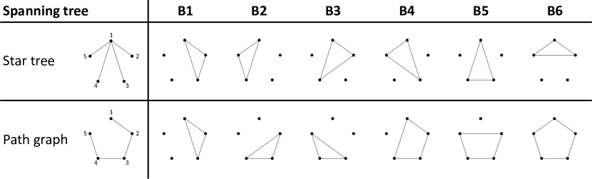
Figure 3: Illustration of two fundamental systems of cycles with $n=5$ vertices.

2.4 Comparing the cycle space with the set of decomposable graphs

As discussed in Section 1, there have been efforts to limit the search space to a subset of $\mathcal{G}_{n}$, most notably to the set of decomposable graphs. While this restriction has the advantage of allowing normalising factors to be computed exactly, there are drawbacks to this restriction especially in applications. Firstly, unlike the cycle space, the set of decomposable graphs is not known to be closed under any vector addition operation. As a result, more involved MCMC algorithms have been proposed to ensure that proposed graphs are decomposable via constraints on which edge to flip [15, 33] or by sampling from the larger set of junction trees, which correspond to decomposable graphs [16]. On the other hand, in the cycle space, we are able to propose moves which are guaranteed to be in $\mathcal{C}_{n}$ by standard properties of vector spaces. Relatedly, decomposability cannot be checked as easily as Property P2 which determines membership of $\mathcal{C}_{n}$.

Another, more important drawback of restricting inference to decomposable graphs is that, in general, decomposable graphs do not approximate other graphs well. For instance, $O(n\log n)$ edges need to be added to a graph to make the resulting graph decomposable in general [8]. This contrast with the cycle space as any graph $G\in\mathcal{G}_{n}$ is at most $n/2$ edges different from a graph in $\mathcal{C}_{n}$ per the following result:

Proposition 2.3

Let $k$ be the number of odd-degree vertices in $G\in\mathcal{G}_{n}$. Then, there exists a graph in $\mathcal{C}_{n}$ that differs from $G$ by $k/2$ edges while there exists no graph in $\mathcal{C}_{n}$ that differs from $G$ by less than $k/2$ edges.

The size of $\mathcal{C}_{n}$ is also larger than that of the set of decomposable graphs. Note that $\mathcal{G}_{n}$ has $2^{n(n-1)/2}$ elements since the standard basis is the edge set containing $n(n-1)/2$ elements. By Property P4, the cardinality of $\mathcal{C}_{n}$ is $2^{(n-1)(n-2)/2}$. In contrast, the number of decomposable graphs on $n$ vertices tends towards $2^{n^{2}/4+O(n\log n)}$ as $n\to\infty$ [5]. (For comparison, the number of spanning trees on the complete graph, which are decomposable, is $|\mathcal{T}_{n}|=n^{n-2}$ by Cayley’s [6] formula.) Thus, constraining graphs to the cycle space is substantially less restrictive than assuming decomposability with a clear upper bound to the difference between any true graph and $\mathcal{C}_{n}$. Lastly, the set of decomposable graphs is not a subset of $\mathcal{C}_{n}$. For instance, trees are not in $\mathcal{C}_{n}$ by Property P2 since their leaf vertices have degree one.

3 Theoretical properties of cycle basis priors

A prior distribution on $\mathcal{C}_{n}$ can be induced by assigning a distribution to cycle basis elements. In this section, we explore the theoretical properties of such priors. Here, $C$ denotes a basis of cycles for $\mathcal{C}_{n}$. Thus, $C$ is a set of $(n-1)(n-2)/2$ cycles. The results hold for any fixed basis $C$ unless otherwise noted. We begin by showing that it is possible to induce the uniform prior on $\mathcal{C}_{n}$.

A cycle basis prior can be defined in terms of cycle-inclusion probabilities. Similarly to the standard basis, when the cycle-inclusion probability is 0.5, we get the uniform prior on $\mathcal{C}_{n}$.

Proposition 3.1

Let $C$ be any cycle basis for the cycle space $\mathcal{C}_{n}$. Suppose that the inclusion of each cycle in $C$ is an independent Bernoulli random variable with probability $0.5$. Then, the induced distribution on $\mathcal{C}_{n}$ is uniform and the marginal edge inclusion probabilities equal $0.5$.

This uniformity holds for any $C$ and thus also for the distribution on $\mathcal{C}_{n}$ induced by a distribution on such bases $C$. The edge inclusions are not independent under the uniform distribution over $\mathcal{C}_{n}$: independent edges with probability $0.5$ yields the uniform distribution over $\mathcal{G}_{n}$. Instead, edge flips can only happen jointly on sets of edges that correspond to graphs in $\mathcal{C}_{n}$ to stay in the cycle space, i.e. to continue to satisfy Property P2.

Often, there is interest in non-uniform distributions, for instance to induce sparsity. In general, the edge inclusion probabilities induced by inclusion probabilities of cycle basis elements depend on the choice of cycle basis, and hence on the choice of spanning tree used to generate this basis via the fundamental system of cycles (Property P3). Although a closed-form expression is not available, we propose an efficient algorithm to compute the edge inclusion probabilities from a cycle basis prior.

Proposition 3.2

Let $e\in\{(i,j)\in V\times V:i<j\}$ be any edge. Let $\{c_{1},\ldots,c_{r}\}\subset C$ be the set of basis elements that contain $e$. Suppose that the inclusions of these elements are independent with inclusion probabilities $\{p_{1},\ldots,p_{r}\}$. Define the polynomial

$$f(x)=\prod_{i=1}^{r}(1-p_{i}+p_{i}x).$$

Then, the induced marginal probability of inclusion of the edge $e$ is the sum of the coefficients of the odd powers of $x$ in $f(x)$. This edge probability reduces to ${\{1-(1-2p)^{r}\}/2}$ if the probabilities $\{p_{1},\ldots,p_{r}\}$ are all equal to $p$.

If the cycle basis is generated from a star tree with independent and equally probable inclusion of basis elements, then these probabilities simplify. (The fundamental system of cycles with respect to a star tree is the set of all cycles of three edges that are incident to its root.)

Corollary 3.3

Let the basis $C$ be defined as the fundamental system of cycles with respect to a star tree $T$ on $n\geq 2$ vertices. Suppose that the cycle inclusions are independent Bernoulli random variables with probability $p$. Then, the marginal edge inclusion probabilities are given by

$$\mathbb{P}\{(i,j)\in E\mid T\}=\begin{cases}\{1-(1-2p)^{n-2}\}/2,&\text{$i$ or $j$ is the root of $T$}\\ p,&\text{otherwise}\end{cases}$$

Moreover, the distribution induced by the uniform distribution over all star trees has $\mathbb{P}\{(i,j)\in E\}=p+\{1-2p-(1-2p)^{n-2}\}/n$.

Polynomial multiplication can be performed efficiently using linear convolution based on a fast Fourier transform (FFT), making the computation of the probabilities in Propostion 3.2 efficient. For the sake of completeness, we also provide an algorithm to compute the joint distribution of edge inclusions induced by the cycle basis prior. This is useful in, for example, calculating the degree distribution of a vertex.

Proposition 3.4

Let $v\in V$ be any vertex. Let $\{e_{1},\ldots,e_{m}\}$ be the set of edges incident to $v$. Let $\{c_{1},\ldots,c_{r}\}\subset C$ be the set of cycles incident to $v$. Suppose that the cycle inclusions are independent with inclusion probabilities $\{p_{1},\ldots,p_{r}\}$. For $i=1,\dots,r$, let $a(i),b(i)\in\{1,\ldots,m\}$ be such that $e_{a(i)},e_{b(i)}$ are the edges of $c_{i}$ that are incident to $v$. Define the polynomial

$$f(t_{1},\ldots,t_{r})=\prod_{i=1}^{r}(1-p_{i}+p_{i}t_{i}).$$

Let $g$ be the image of $f$ in the polynomial ring $\mathbb{R}[x_{1},\ldots,x_{m}]/\langle x_{1}^{2},\ldots,x_{m}^{2}\rangle$ under the unique ring homomorphism satisfying $t_{i}\mapsto x_{a(i)}x_{b(i)}$. Then, the probability of including any set of edges $\{e_{s}\}_{s\in S}$ while excluding the other $m-|S|$ edges incident to $v$ is given by the coefficient of $\prod_{s\in S}x_{s}$ in $g$.

The above proposition can be applied in practice by noting that $g$ is equal to the product of the polynomials $1-p_{i}+p_{i}x_{a(i)}x_{b(i)}$ in the ring $\mathbb{R}[x_{1},\ldots,x_{m}]/\langle x_{1}^{2},\ldots,x_{m}^{2}\rangle$. Multiplication of linear polynomials modulo squares is equivalent to a circular convolution. By the circulant convolution theorem, this can be efficiently performed using an FFT of length 2 in $m$ dimensions.

Although the above algorithm can be used to calculate degree distributions in the general case, closed-form expressions may be computed when the spanning tree used to generate the cycle basis has a tractable structure as in the case of star trees.

Proposition 3.5

Let the basis $C$ be defined as the fundamental system of cycles with respect to the star tree on the vertices $\{v_{0},\ldots,v_{n-1}\}$, $n\geq 2$, rooted at $v_{0}$. Suppose that the cycle inclusions are independent Bernoulli random variables with probability $p$. Then, the degree distribution for the vertices $\{v_{1},\dots,v_{n-1}\}$ is given by

$$\mathbb{P}\{\deg(v_{i})=k\}=\begin{cases}(1-p)^{n-2},&k=0\\ \sum_{j=k-1}^{k}\binom{n-2}{j}p^{j}(1-p)^{n-2-j},&\text{$2\leq k<n$ and $k$ is even}\\ 0,&\text{otherwise}\end{cases}$$

We now briefly discuss the sparsity of graphs in the cycle space. For a given probability $p$ of independent basis element inclusions, Proposition 3.2 gives the edge probability $\{1-(1-2p)^{r}\}/2$ which is an increasing function of $p$ for $p\leq 0.5$ and which involves the number $r$ of elements in the basis $C$ that include the edge. Thus, setting a smaller $p$ yields shrinkage on the number of edges: the edge probability can be made arbitrarily small via $p$. This shrinkage depends on $C$ via $r$. For instance, consider Figure 3 and edge $(2,3)$. There, $r=1$ for $C$ generated by the star tree and $r=5$ for $C$ generated by the path graph. In general, $r=1$ for any edges in the complement $\overline{T}$ of the spanning tree $T$ that generated $C$. For edges in $T$, $r$ varies with $C$.

More generally, there is no simple relationship between the sparsity of a graph in terms of its cycle basis inclusions and the edge-sparsity of that graph. However, analytical results are available in the particular case that the cycle basis is generated from a star tree.

Proposition 3.6

Let the basis $C$ be defined as the fundamental system of cycles with respect to a star tree on $n$ vertices. Define $m=\lfloor(n-1)/2\rfloor$. Consider the graph $G=(V,E)$ formed by the inclusion of ${q}$ basis elements from $C$. Then, the number of edges $|E|$ is bounded as ${q}\leq|E|\leq{q}+2\min({q},\,m)$. The upper bound is tight for ${q}\leq m$.

This implies that specifying a shrinkage prior on ${q}$ leads to shrinkage on the number of included edges for cycle bases induced by a star tree. We also consider $|E|$ as a function of ${q}$ empirically in Figure 4. The empirical results show that a number ${q}$ implies a smaller range of $|E|$ than suggested by Proposition 3.6, especially for a large number of vertices.

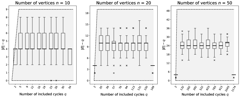
Figure 4: Box plots of $|E|-{q}$ from 100 graphs $G$ generated by sampling ${q}$ elements from a basis $C$ generated by a star tree without replacement. The dashed lines mark the bounds $0\leq|E|-{q}\leq 2\min({q},\,m)$ from Proposition 3.6.

Simulation studies in Section 4 confirm that limiting $q$ also results in lower posterior edge inclusion probabilities, as does lowering the prior basis element inclusion probability $p$.

Apart from the prior process on cycle bases, we also consider the prior induced by edge unions of spanning trees in Supplementary Material. However, we find that computation of the induced prior $p(G)$ is intractable since edge unions of spanning trees do not form a vector space. We propose an algorithm to compute $p(G)$, specifically to count the number of decompositions of a graph into spanning trees, with complexity $O(2^{|E|}\,n^{3})$ which is an improvement over the superexponential complexity of the brute-force enumeration method. Further, we prove bounds to attempt an approximation of the prior ratio as appearing in a Metropolis-Hastings acceptance probability, but simulations shows that the bounds are too wide be of use (see Supplementary Material).

4 Simulation studies with the cycle basis prior

We conduct simulation studies to better understand what the effect of certain cycle basis priors on posterior inference is. We do not apply these priors to the gene expression application in Section 5 as the decomposition of a graph into changing cycle bases in Step LABEL:supp:step:decomposition of Algorithm LABEL:supp:alg:MCMC in Supplementary Material is too expensive with $n=93$ vertices. We simulate the $N\times n$ data matrix $X$ from the model $p(X\mid K)$ in (1) with the $n\times n$ precision matrix $K$ given by $K_{ii}=1$ for $i=1,\dots,n$ and $K_{12}=K_{13}=K_{23}=K_{34}=K_{35}=K_{45}=0.3$ while all other upper-triangular elements of $K$ equal zero. This fully defines $K$ as it is a symmetric matrix. Thus, the true underlying graph $G$ corresponds to the union of the two cycles $(1,2,3)$ and $(3,4,5)$. We set $n=15$ as number of vertices and $N=150$ as number of observations.

We consider six different priors on graphs. The first one is the edge basis prior with independent edge inclusions with probability $p=0.5$. The next four priors are constrained to the cycle space $\mathcal{C}_{n}$ as follows. The second prior is induced by the uniform prior $p(T)$ over all spanning trees combined with the prior $p(G\mid T)$ resulting from a priori independent basis element inclusions with probability $p=0.5$ where the cycle basis is generated by spanning tree $T$. The third prior uses the same uniform $p(G\mid T)$ but with $p(T)$ uniform over all star trees instead of the larger set of all spanning trees. The fourth prior is the same as the third prior but with a different $p(G\mid T)$ where the a priori basis element inclusion probability is $p=0.05$ instead of $0.5$. The fifth prior is like the third prior but with $p(G\mid T)$ uniform over all graphs that consist of $q=3$ or fewer elements from the cycle basis generated by $T$. Finally, the last prior is uniform over all decomposable graphs.

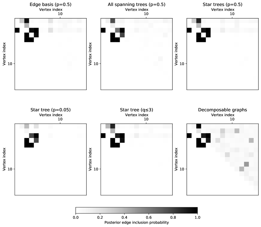
Figure 5: The posterior edge inclusion probabilities (upper triangle) and the median probability graph (lower triangle) resulting from the six different priors considered for the simulated data.

We compute the posterior for the first five priors using Algorithm LABEL:supp:alg:MCMC in Supplementary Material where we repeat Step LABEL:supp:step:update_G nine times for each Step LABEL:supp:step:update_T. Step LABEL:supp:step:update_T involves sampling from $p(T)$. For the uniform prior over all spanning trees (the second prior), we use the algorithm from [1] to sample from $p(T)$. Schild [29] provides a faster alternative. We set the total number of MCMC steps, i.e. executions of Algorithm LABEL:supp:alg:MCMC, to $10^{5}$ of which $10^{4}$ as burn-in. Posterior computation for the prior on decomposable graphs is as described in Section 5. Figure 5 visualises the resulting posterior edge inclusion probabilities. The probabilities are not notably different between the edge basis and the uniform prior over the cycle space $\mathcal{C}_{n}$ induced by considering all spanning trees or all star trees with $p=0.5$.

The median probability graphs of the first three priors plus the star tree prior with the number of basis elements $q$ capped at three ($q\leq 3$) have identical recovery of the true underlying graph with the cycle $(3,4,5)$ and edge $(1,3)$ correctly detected, failure to detect $(1,2)$ and $(2,3)$, and no false positives. The extra prior regularisation in the fourth prior with $p=0.05$ results in edge $(1,3)$ not being detected. The truncation $q\leq 3$ in the fifth prior results in lower inclusion probabilities: an average probability of $0.054$ compared to $0.056$ for the third prior with $p=0.5$. The fourth prior with $p=0.05$ yields yet a lower average probability at $0.033$. The prior on decomposable graphs produces an average of 0.11 with notably non-zero probabilities also for edges with endpoints outside of the first five nodes.

5 Application to gene expression data

In this section, we restrict the graph space $\mathcal{G}_{n}$ to the cycle space $\mathcal{C}_{n}$ while inferring a gene expression network. The data are gene expression profiles taken from tumours of breast cancer patients obtained from the R package gRbase [11] preprocessed following the procedure in [17] which yields $n=93$ genes of interest from $N=250$ patients. For a further description of the data collection, see [23].

For this application, we consider three priors on $\mathcal{G}_{n}$: the uniform prior on $\mathcal{G}_{n}$ corresponding to the standard “edge” basis, the uniform prior on $\mathcal{C}_{n}$ such as arising from a cycle basis (e.g. Proposition 3.1) and a uniform prior over all decomposable graphs. We use a Metropolis-Hastings algorithm for posterior inference where the proposal is to flip the presence of one basis element in $G$ where we use the edge basis also for the prior on decomposable graphs. For the cycle basis, this proposal is guaranteed to be in $\mathcal{C}_{n}$ as a vector space is closed under addition. See Section LABEL:supp:sec:mcmc_uniform of Supplementary Material for details of the MCMC. The computational cost is similar for the edge and cycle basis. Since the Metropolis-Hastings proposal that we use for decomposable graphs is not constrained to decomposable graphs, the rejection rate of that MCMC is high. We therefore run it for longer than the MCMC with the edge and cycle basis.

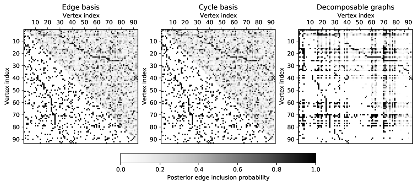
Figure 6: The posterior edge inclusion probabilities (upper triangle) and the median probability graph (lower triangle) resulting from the standard edge basis (left), cycle basis (centre) and the set of decomposable graphs (right).

Figure 7: Graphs obtained by including edges whose posterior inclusion probability is larger than $0.95$ when using the standard edge basis (left) and the cycle basis (right). The left graph has 141 edges and the right graph has 147 edges, 123 of which appear in both graphs.

Table 1: Minimum, average and maximum absolute difference in posterior edge inclusion probabilities resulting from the cycle basis and the set of decomposable graphs relative to the standard edge basis.

	Minimum	Average	Maximum
Cycle basis	0.00	0.04	0.33
Decomposable graphs	0.00	0.19	1.00

Figures 6 and 7, and Table 1 summarise the resulting graph inference. There is no major difference between the posterior edge inclusion probabilities with the edge basis and the cycle basis. This is despite the cycle space restriction with the cycle basis. These results suggest that restricting inference to the cycle space $\mathcal{C}_{n}\subset\mathcal{G}_{n}$ does not substantially affect posterior inference from when the graph space $\mathcal{G}_{n}$ is not restricted. This contrasts with the results for decomposable graphs which are substantially different from both the edge and cycle basis results, reflecting that decomposability is a more severe restriction than the cycle space.

6 Discussion

In this paper, we introduce a generalisation of the edge inclusion prior based on vector spaces and, in particular, investigate the cycle subspace. We present theoretical results about the cycle space and their bases. While the results presented in Section 2 are not our own except for Proposition 2.3, to the extent of our knowledge, this is the first time the idea of restricting inference to the cycle space is introduced in the graphical model literature.

We also study a novel prior based on assigning independent prior basis inclusion probabilities, proving its degree distribution and shrinkage properties. We implement an MCMC algorithm that samples from the cycle space. Our algorithm is more straightforward to implement when compared to methods for decomposable graphs [15, 16, 33], by the fact that vector spaces are closed under addition. We show empirically that studying a smaller but dense subset of the graph space does not significantly affect inference of posterior edge inclusion probabilities.

Moreover, this paper opens up an opportunity to various extensions of existing methodologies by considering alternative graph vector spaces such as induced by cycle bases as opposed to the edge basis. For example, the size-based prior of Armstrong et al. [2] can be used to shrink to the number of basis elements. Also, a birth-death proposal on the basis elements can be used instead of the proposal used in this paper that randomly switches one basis element selected from a uniform distribution on all elements.

Lastly, in this paper, we only considered standard GGMs. However, it may be possible to extend this method to other types of graphical models such as multiple graphs [27, 34], Gaussian copulas [12, 24] and chain graphs [32, 22].

This work was supported by the Singapore Ministry of Education Academic Research Fund Tier 2 under Grant MOE2019-T2-2-100.

There were no competing interests to declare which arose during the preparation or publication process of this article.

The data related to the application in Section 5 can be found at https://github.com/kristoforusbryant/cbmcmc/blob/main/breastcancer/data/breastcancer_data_93_250.csv.

The supplementary material for this article can be found at http://doi.org/10.1017/[TO BE SET].

References

- [1] Aldous, D. J. (1990). The random walk construction of uniform spanning trees and uniform labelled trees. SIAM J. Discrete Math. 3, 450–465.
- [2] Armstrong, H., Carter, C. K., Wong, K. F. K. and Kohn, R. (2009). Bayesian covariance matrix estimation using a mixture of decomposable graphical models. Statist. Comput. 19, 303–316.
- [3] Atay-Kayis, A. and Massam, H. (2005). A Monte Carlo method for computing the marginal likelihood in nondecomposable Gaussian graphical models. Biometrika 92, 317–335.
- [4] Axler, S. (2015). Linear Algebra Done Right 3rd ed. Undergraduate Texts in Mathematics. Springer Cham, Heidelberg. Theorem 2.33.
- [5] Bender, E., Richmond, L. and Wormald, N. (1985). Almost all chordal graphs split. J. Austral. Math. Soc. 38, 214–221.
- [6] Cayley, A. (1889). A theorem on trees. Q. J. Pure Appl. Math. 23, 376–378.
- [7] Chaiken, S. and Kleitman, D. J. (1978). Matrix tree theorems. J. Comb. Theory Ser. A 24, 377–381.
- [8] Chung, F. R. and Mumford, D. (1994). Chordal completions of planar graphs. J. Comb. Theory Ser. B 62, 96–106.
- [9] Dawid, A. P. and Lauritzen, S. L. (1993). Hyper Markov laws in the statistical analysis of decomposable graphical models. Ann. Statist. 21, 1272–1317.
- [10] Dempster, A. P. (1972). Covariance selection. Biometrics 28, 157–175.
- [11] Dethlefsen, C. and Højsgaard, S. (2005). A common platform for graphical models in R: The gRbase package. J. Statist. Softw. 14, 1–12.
- [12] Dobra, A. and Lenkoski, A. (2011). Copula Gaussian graphical models and their application to modeling functional disability data. Ann. Appl. Statist. 5, 969–993.
- [13] Duan, L. L. and Dunson, D. B. Bayesian spanning tree: Estimating the backbone of the dependence graph 2021. arXiv:2106.16120v1.
- [14] Giudici, P. (1996). Learning in graphical Gaussian models. In Bayesian Statistics 5. ed. J. M. Bernardo, J. O. Berger, A. P. Dawid, and A. F. M. Smith. Oxford University Press, Oxford. pp. 621–628.
- [15] Giudici, P. and Green, P. J. (1999). Decomposable graphical Gaussian model determination. Biometrika 86, 785–801.
- [16] Green, P. J. and Thomas, A. (2013). Sampling decomposable graphs using a Markov chain on junction trees. Biometrika 100, 91–110.
- [17] Højsgaard, S., Edwards, D. and Lauritzen, S. (2012). Graphical Models with R. Springer, New York.
- [18] Jones, B., Carvalho, C., Dobra, A., Hans, C., Carter, C. and West, M. (2005). Experiments in stochastic computation for high-dimensional graphical models. Statist. Sci. 20, 388–400.
- [19] Kruskal, J. B. (1956). On the shortest spanning subtree of a graph and the traveling salesman problem. Proc. Amer. Math. Soc. 7, 48–50.
- [20] Lauritzen, S. L. (1996). Graphical Models. Oxford Statistical Science Series. The Clarendon Press, Oxford University Press, New York.
- [21] Lenkoski, A. and Dobra, A. (2011). Computational aspects related to inference in Gaussian graphical models with the -Wishart prior. J. Comput. Graph. Statist. 20, 140–157.
- [22] Lu, D., De Iorio, M., Jasra, A. and Rosner, G. L. (2020). Bayesian inference for latent chain graphs. Found. Data Sci. 2, 35–54.
- [23] Miller, L. D., Smeds, J., George, J., Vega, V. B., Vergara, L., Ploner, A., Pawitan, Y., Hall, P., Klaar, S., Liu, E. T. and Bergh, J. (2005). An expression signature for p53 status in human breast cancer predicts mutation status, transcriptional effects, and patient survival. Proc. Natl. Acad. Sci. U.S.A. 102, 13550–13555.
- [24] Mohammadi, R. and Wit, E. C. (2019). BDgraph: An R package for Bayesian structure learning in graphical models. J. Statist. Softw. 89, 1–30.
- [25] Murray, I., Ghahramani, Z. and MacKay, D. J. C. (2006). MCMC for doubly-intractable distributions. In Proceedings of the Twenty-Second Conference on Uncertainty in Artificial Intelligence. UAI’06. AUAI Press, Arlington, Virginia, USA. p. 359–366.
- [26] Niu, Y., Pati, D. and Mallick, B. K. (2021). Bayesian graph selection consistency under model misspecification. Bernoulli 27, 637–672.
- [27] Peterson, C., Stingo, F. C. and Vannucci, M. (2015). Bayesian inference of multiple Gaussian graphical models. J. Am. Statist. Assoc. 110, 159–174.
- [28] Roverato, A. (2002). Hyper inverse Wishart distribution for non-decomposable graphs and its application to Bayesian inference for Gaussian graphical models. Scand. J. Statist. 29, 391–411.
- [29] Schild, A. (2018). An almost-linear time algorithm for uniform random spanning tree generation. In Proceedings of 50th Annual ACM SIGACT Symposium on the Theory of Computing (STOC’18). pp. 214–227.
- [30] Schwaller, L., Robin, S. and Stumpf, M. (2019). Closed-form Bayesian inference of graphical model structures by averaging over trees. Journal de la Société Française de Statistique 160, 1–23.
- [31] Scott, J. G. and Carvalho, C. M. (2008). Feature-inclusion stochastic search for gaussian graphical models. J. Comput. Graph. Statist. 17, 790–808.
- [32] Sonntag, D. and Peña, J. M. (2015). Chain graphs and gene networks. In Foundations of Biomedical Knowledge Representation. SpringerNature, Switzerland pp. 159–178.
- [33] Stingo, F. and Marchetti, G. M. (2015). Efficient local updates for undirected graphical models. Statist. Comput. 25, 159–171.
- [34] Tan, L. S., Jasra, A., De Iorio, M. and Ebbels, T. M. (2017). Bayesian inference for multiple Gaussian graphical models with application to metabolic association networks. Ann. Appl. Statist. 11, 2222–2251.
- [35] Uhler, C., Lenkoski, A. and Richards, D. (2018). Exact formulas for the normalizing constants of Wishart distributions for graphical models. Ann. Statist. 46, 90–118.
- [36] van den Boom, W., Jasra, A., De Iorio, M., Beskos, A. and Eriksson, J. G. (2022). Unbiased approximation of posteriors via coupled particle Markov chain Monte Carlo. Statist. Comput. 32, 36.
- [37] Veblen, O. (1912). An application of modular equations in analysis situs. Ann. of Math. 14, 86–94.
- [38] Wallis, W. D. (2010). A Beginner’s Guide to Graph Theory. Springer Science+Business Media, New York.
- [39] Wang, H. and Carvalho, C. M. (2010). Simulation of hyper-inverse Wishart distributions for non-decomposable graphs. Electron. J. Statist. 4, 1470–1475.
- [40] Wang, H. and Li, S. Z. (2012). Efficient Gaussian graphical model determination under -Wishart prior distributions. Electron. J. Statist. 6, 168–198.