Learning A Simulation-based Visual Policy for Real-world Peg In Unseen Holes

Abstract

This paper proposes a learning-based visual peg-in-hole that enables training with several shapes in simulation, and adapting to arbitrary unseen shapes in real world with minimal sim-to-real cost. The core idea is to decouple the generalization of the sensory-motor policy to the design of a fast-adaptable perception module and a simulated generic policy module. The framework consists of a segmentation network (SN), a virtual sensor network (VSN), and a controller network (CN). Concretely, the VSN is trained to measure the pose of the unseen shape from a segmented image. After that, given the shape-agnostic pose measurement, the CN is trained to achieve generic peg-in-hole. Finally, when applying to real unseen holes, we only have to fine-tune the SN required by the simulated VSN+CN. To further minimize the transfer cost, we propose to automatically collect and annotate the data for the SN after one-minute human teaching. Simulated and real-world results are presented under the configurations of eye-to/in-hand. An electric vehicle charging system with the proposed policy inside achieves a 10/10 success rate in 2$\sim$3s, using only hundreds of auto-labeled samples for the SN transfer.

I Introduction

Figure 1: Conceptual illustration of the precision peg-in-hole. The peg is mounted on the end-effector of the manipulator whose motion is guided by an image-based sensor, as shown in (a). The vision-based solution is particularly preferred in this work, because of its ability to capture the global scene information as well as the semantic and geometric object properties. The training process of any algorithm can only be carried out within a limited set of peg shapes, shown in (b), while in practical the shape of the peg to be manipulated may be arbitrary, such as the testing cases shown in (c). This work aims to propose a framework for precision peg-in-hole towards easy generalization to arbitrary unseen shapes.

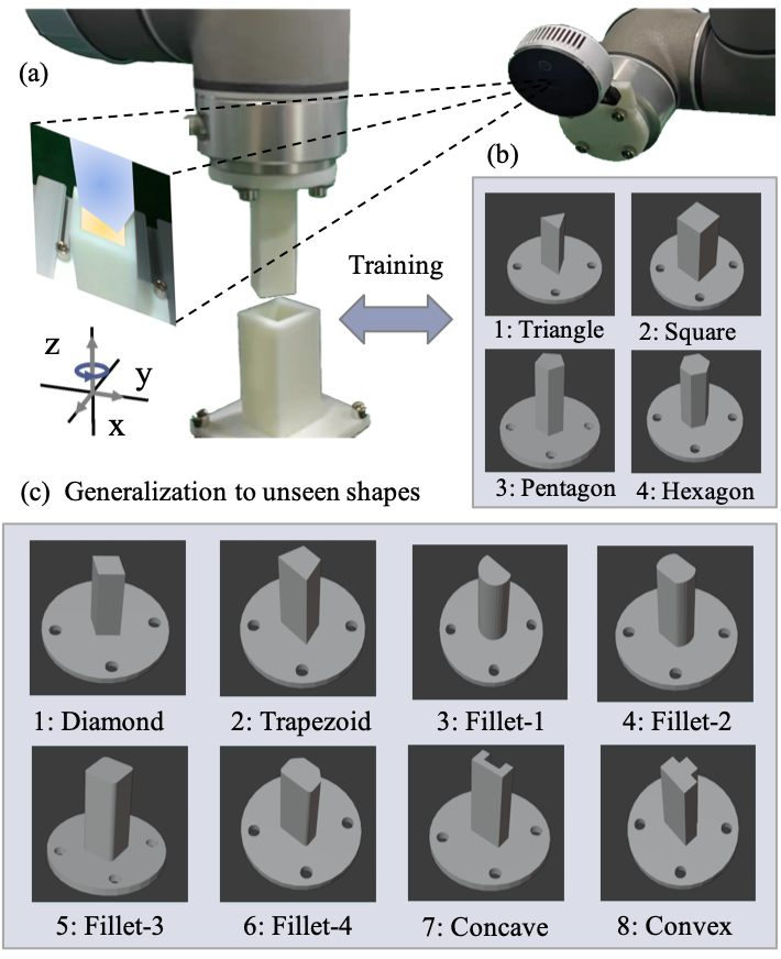
Robotic peg-in-hole [1] is a routine skill with a wide spectrum of applications ranging from industrial manufacturing to recently human’s daily housework, such as placing the key into the lock and inserting the bolt into the nut. In these applications, the shapes of the peg/hole to be manipulated may be arbitrary and unseen in prior, thus developing the capability to deal with unseen shapes becomes non-trivial for all existing peg-in-hole solutions. An expected learning scenario is that the policy is trained with several shapes, and tested to another set of shapes unseen in the training set, see Fig. 1 for illustration. In this way, the robot can better adapt to the diverse demands, e.g. an electric vehicle (EV) charging robot is able to handle new protocols of charging interface without additional expert programming.

Towards the goal, the existing force-based insertion policies have achieved a high success rate for holes with sub-$mm$ tolerance, given the initial misaligned error of about 1$mm$ [2]. But it fails when the initial error becomes larger. One recent work [3] pushes the robustness against the initial error up to 4$mm$ and 4^∘, with the cost that the generalization is achieved by model fine-tuning using additional task-specific human demonstration trajectories. The insight of this work is the generalization scenario that the policy is trained with several shapes, and tested to another set of shapes unseen in the training set, with an additional non-expert cost. Despite the scenario pushing both the generalization and the robustness against the initial error, the performance of force-based policy is still insufficient in mobile manipulation tasks due to the relatively large base navigation error.

The vision-based policy is another option, which has the potential to correct the error and make fewer peg-hole contacts. Existing vision-based works [4] provide mature solutions for holes with 1$mm$ tolerance, which is acceptable for many applications. If sub-$mm$ is required, one can simply employ a follow-up force-based insertion [5]. However, vision-based methods highly depend on manual feature extraction, error modeling, and controller design, struggling to deal with unseen objects. Recent progress in multi-modal representation shows promising results [6], but still faces difficulty to achieve 1$mm$ level precision.

To address the above problem, we propose to bring the generalization to the vision-based policy for holes with 1$mm$ tolerance, from $\sim$10$mm$ initial error. The vision generalization is inspired that the policy is trained with several shapes, and tested to another set of shapes unseen in the training set, with minimal additional cost, which is a one-minute human pose teaching. The core idea is to decouple the generalization of the sensory-motor policy to the design of a fast-adaptable perception module and a simulation-based generic policy module. The decoupling is achieved by introducing a segmented image in between. As a result, a framework for the peg-in-hole tasks is proposed, consisting of a segmentation network (SN), a virtual sensor network (VSN), and a controller network (CN). Under this framework, the segmented image-based policy (VSN+CN) is trained totally in simulation, which can perform generic insertion given a peg-hole segmented image, replacing the unsafe and time-consuming real-world training as some force-based policy [5]. The fast-adaption of the perception is achieved by fine-tuning the SN only using hundreds of images. To minimize this additional cost, an automatic data collection and annotation pipeline for image segmentation is designed, which only needs a one-minute human pose teaching. Note that the human effort in this scenario is almost minimal, as it is the same as the traditional position-based robot application. Finally, by connecting the modules, the vision-based policy can be applied to real-world peg-in-hole tasks. In summary, the contributions are as follows:

• A vision-based peg-in-hole policy framework that decouples the generalization of the sensory-motor policy to the design of a fast-adaptable perception module and a simulation-based generic policy module.

• A segmented-image based insertion policy with VSN and CN, trained totally in simulation, is able to generalize to peg in unseen holes.

• An automatic data collection and annotation pipeline for image segmentation, leverages one-minute human teaching for fast-adaptable perception.

• Extensive experiments validating the 1$mm$ level performance of the policy, both in the configuration of eye-to-hand and eye-in-hand, as well as a real-world peg insertion application in the EV charging system. Code is released at https://github.com/xieliang555/SFN.git.

The article is an extension work of previously published conference paper [7]. We extend the proposed framework to the eye-in-hand configuration, where we find that the visual state may remain unchanged for several consecutive image frames under visual occlusion circumstances. Thus in the multi-frame policy, we consider the extra action cues to reduce the uncertainties, with all the experiments conducted in both the configuration of eye-to-hand and eye-in-hand. We systematically ablate each module of the proposed framework by comparing the VSN policy, the single-frame policy, and the multi-frame policy. We also compare three different adaptation strategies to demonstrate the characteristic of fast adaptation with minimal manual cost. Finally, we extend the proposed framework to the real-world automatic EV charging system. By fine-tuning the SN module with only 10 epochs on hundreds of images, the proposed framework can be quickly adapted to the unseen EV charging scenarios with 10/10 success rate, which demonstrates the effectiveness and practicability.

The remainder of this paper is organized as follows: Related works are reviewed in Sec. II. The proposed method is detailed in Sec. III. The controller design is presented in Sec. IV. Implementations can be found in Sec. V. Sec. VI provides the simulations and real-world experiments. Finally, Sec. VII concludes the article.

II Related Work

II-A Peg-in-hole Assembly

Robotic peg-in-hole has been studied for several decades from numerous viewpoints, which raises many challenges. Conventional line of work like spiral search [8] exhaustively locates the hole within an uncertain region following the predefined (scripted) trajectories. However, the long-time contact-rich searching may hurt the surface quality of the peg-hole pairs. Model-based insertions [9] rely on contact model analysis to reason about state conditions and decompose the peg-in-hole tasks into two steps: contact state recognition and compliant control. These algorithms typically either use force/torque signals to detect peg-hole interactions [10] or leverage vision for pose information [4], based on which optimal insertion trajectories are planned. To overcome the uncertainty in sensing and modeling, compliance control is often applied to the manipulator [11]. Principally, these work can achieve fast insertion with less contact, but struggle to generalize to new insertion scenarios due to the task-specific design in perception modeling, planning, and control.

Recently with the progress of deep learning, another line of work focus on learning-based methods for the insertion tasks. [5] achieves high-precision assembly on a tight clearance cylindrical peg-in-hole task by training a reinforcement learning (RL) policy in real-world. The precision required to perform this task exceeds that of robots. But the extensive number of contact-rich interactions increase the possibility to damage the environment and the robot itself, and the learned policy only applies to the cylindrical peg/hole. To improve sample efficiency and generalization, the human-in-the-loop demonstration has been incorporated as prior information to the RL algorithms [3]. However, it takes a long time to transfer the skills to the unseen insertion tasks by online fine-tuning, which hinders the algorithms from quickly scaling up to the real-world unseen insertions. [6] shows the potential to generalize over varying geometries by learning a multisensory representation in simulation, based on which an RL-based policy is trained in the real world, which demonstrates to improve the sample efficiency of the policy learning. However, the selected tasks do not require the policy to be as precise as industrial connector insertions.

Figure 2: The proposed vision feedback framework. (a) Automatic data collection and annotation pipeline to accelerate the perception adaptation. (b) SN: peg-hole segmentation network to transfer the raw RGB image to the segmented image. (c) VSN: general position and rotation feature extraction based on the segmented image. (d) The decoupled motion-force control to generate robot command, where the motion control is achieved by the proposed CN.

II-B Data Collection and Sim-to-real

The leading learning-based approaches for contact-rich manipulations [12, 13], such as peg assembly [14] and fastening screws [15], face the notoriously data-hungry problem [16], where the mechanism for learning abstract policies is lacked through explicit, verbal definition in a few trials like human beings, and work best when there are millions or even billions of training data [17]. Unfortunately, currently, few methods have access to big data because acquiring data involves a process that is labor-intensive, computationally expensive and time-consuming [18, 19, 20, 21]. In [22], a large number of data are obtained with complex synthetic image generation and a lot of manual design. In [23], high-quality and diverse data are obtained with human demonstrations, which proves to broadly improve the performance of the robotic learning tasks. To reduce manual effort, efficient self-supervised data collection has been introduced for offline robot learning with task-relevant loss functions [24, 25]. Alternatively, online data collection without manual intervention can be achieved through robot interactions with the environments [26]. Despite progress, it takes a long time to obtain millions of data in the real world. Furthermore, the wide range of random sampling from trial and error is unsafe for both the contact environment and the robot itself [27].

Simulation is leveraged to improve sample efficiency and safety in the data collection process [28, 29, 30] but also inducts the challenge of the reality gap. [31, 32, 33] achieve sim-to-real with domain randomization by exhaustively choosing the parameters to randomize over to make the simulation as realistic as possible. [34] propose an inverse dynamic model which is learned with the force/torque data generated in a sample-efficient offline fashion. To achieve sim-to-real, the dynamic model is fine-tuned and transferred to new peg-in-holes in real world after a small number of insertion trials. Our proposed method leverages the simulation for most training, and transfers to real world with efficient supervised learning. Only hundreds of images are required for the adaptation, which are collected and annotated safely and automatically with contact-free manipulations in 15 minutes.

II-C Vision Feedback Manipulation

With recent advances in computer vision [35], a lot of prior work focuses on learning an end-to-end visuomotor controller that directly maps raw pixel observations to control actions and closes the control loop with vision feedback [36]. They have shown impressive success in exploring high-dimensional environments to learn complex robot manipulation tasks. However, these end-to-end algorithms require a large amount of training data and remain difficult to generalize to new scenarios without extensive fine-tuning. Borrowing the idea from another line of research that decouples the system into individual sensing and control policy [6], our system is separated into a visual perception module and a generic policy module by a segmentation network in between, based on which the policy generalization problem is transferred to the perception adaptation. While many of these methods introduce the decoupling mechanism with the aim to better incorporate the state-of-the-art vision-based techniques [11, 33, 4] (e.g. pose estimation and tracking, etc.), we instead leverage it as a way to achieve the two sub-tasks: simulated generic policy and fast sim-to-real.

Some vision-based algorithms are limited to the eye-to-hand configuration in order to obtain the robust depth information [25], and many other methods require the camera to move with the robot arm for active sensing [37], which only fits the eye-in-hand configuration. Our method, in contrary, applies to broader application scenarios where the camera can be mounted under either the eye-to-hand or eye-in-hand configurations.

Figure 3: (a) The VSN for position feature extraction. (b) The VSN for rotation feature extraction. (c) The CN for insertion trajectory planning. All modules are learned in simulation.

III Methods

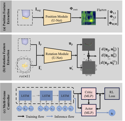
The proposed framework integrates the following modules to complete real-world insertion tasks for peg in unseen holes: a fast-adaptable perception module and a simulation-based generic policy module. As depicted in Fig. 2, the generic policy consists of a VSN and a CN for insertion tasks, which are trained solely in simulation. Then given an unseen real-world insertion task, only the SN has to be fine-tuned, to transfer the RGB image to the segmented image and provide feedback for the control loop. To further accelerate the adaptation, an automatic data collection and annotation pipeline for the SN is proposed. The following subsections describe these components in detail.

III-A Virtual Sensor Network

The VSN functions as a virtual sensor that tries to extract the position and rotation features respectively for pose alignment. Loss functions are delicately designed with inductive bias introduced to encourage the VSN to learn the related features. We represent the features based on spatial heatmaps, which allow for better spatial generalization than directly regressing point coordinates or angles from a latent representation as shown in [38].

III-A1 Position Feature Extraction

Uses a deep neural network that takes the segmented image $\mathbf{I}_{\rm seg}$ as input. $\mathbf{I}_{\rm seg}$ only contains the pixels of the peg, the hole and, the background, which can be obtained from simulation directly. The spatial heatmaps are generated to predict the peg-centric (eye-in-hand) or the hole-centric (eye-to-hand) 2D planar displacement. As shown in Fig. 3(a), the position of the brightest point indicates the relative pose between the peg and the hole. We choose U-Net [39] $f_{\varphi}$ parameterized by $\varphi$ as the backbone to predict the 2-channel one-hot heatmaps from $\mathbf{I}_{\rm seg}$ in Eq. 1:

$$\mathbf{\Phi}=f_{\varphi}(\mathbf{I}_{\rm seg})$$ (1)

Let $dx^{*}$ and $dy^{*}$ be the ground truth of pixel planar displacement along the X-axis and Y-axis respectively, which can be calculated by projecting from the 3D world coordinates with the calibrated camera intrinsic and extrinsic matrices. Then the desired pixel value $\mathbf{\Phi}_{\rm i,j}^{*}$ can be defined in Eq. 2, where $i,j$ are the pixel coordinates of the ground truth heatmaps with the image center to be the coordinate origin.

$$\mathbf{\Phi}_{\rm i,j}^{*}=\begin{cases}1&\text{if $i=dx^{*}$, $j=dy^{*}$}\\ 0&\textit{o.w.}\end{cases}$$ (2)

The loss function is defined over the ground truth heatmaps $\mathbf{\Phi}^{*}$ and the predicted heatmaps $\Phi$ with binary cross entropy loss as in Eq. 3.

$$Loss_{\varphi}=-\sum(\mathbf{\Phi}^{*}\cdot\log\mathbf{\Phi}+(1-\mathbf{\Phi}^{*})\cdot\log(1-\mathbf{\Phi}))$$ (3)

The heatmap can be leveraged not only as the value function as in RL, where we can extract the policy (defined as the VSN policy) for position alignment, but also as the features with uncertainty for the CN (detailed in III-B). For the inference of the VSN policy, the point with the largest value in the produced heatmap is selected as the predicted point, whose indexes are the corresponding translate $dx,dy$ as:

$$dx,dy=\mathop{\arg\max}\limits_{i,j}\mathbf{\Phi}_{\rm i,j}$$ (4)

To obtain the features for the CN, the 2D heatmap is flattened to the 1D vector as defined in Eq. 5.

$$\mathbf{v}=\left\{\mathbf{\Phi}_{\rm i,j}|i,j\in\mathbb{N},i,j\in[0,M)\right\}$$ (5)

where $\mathbf{\Phi}$ is the pixel value of the heatmap, and $M$ indicates the spatial size of the heatmap.

III-A2 Rotation Feature Extraction

Uses the U-Net $f_{\psi}$ as the backbone which consists of a two-stream Siamese network [40] with shared parameters $\psi$ (see Fig. 3(b)). The first stream takes as input the segmented image $\mathbf{I}_{\rm p}$ which only contains the pixels of the peg and the background. The second stream takes as input the 11 rotated segmented images $\mathbf{I}_{\rm h}^{\rm i}$ which only contain the pixels of the hole and the background, with 5 equispaced clockwise rotations and 5 equispaced anticlockwise rotations. Both streams output feature maps with the same resolution as the input, defined as $\mathbf{u}_{\rm p},\mathbf{u}_{\rm h}$ respectively. The $11\times 1$ feature vector produced by the rotation module is defined as:

$$\mathbf{u}_{\rm p}=f_{\psi}(\mathbf{I}_{\rm p})$$ (6)

$$\mathbf{u}_{\rm h}^{\rm i}=f_{\psi}(\mathbf{I}_{\rm h}^{\rm i})$$ (7)

$$\mathbf{d}=\left\{e^{-d(\mathbf{u}_{\rm p},\mathbf{u}_{\rm h}^{\rm i})}|i\in\mathbb{N},i\in[0,11)\right\}$$ (8)

where $d$ is the Euclidean distance between the two feature maps. Among the 11 rotated images $\mathbf{I}_{\rm h}^{\rm i}$, only the correct one $\mathbf{I}^{\rm p}_{\rm h}$ with the ground-truth rotation will match $\mathbf{I}_{\rm p}$ and the others $\mathbf{I}^{\rm n}_{\rm h}$ will mismatch. To establish the rotation correspondences between the peg and the hole, a variant triplet loss function [41] is designed to encourage the paired feature maps to match, while pushing the unpaired maps apart. By constraining the feature distance (defined in Eq. VII) in the range of $(0,1]$, the paired feature distance $\mathbf{d}_{\rm p}$ is expected to be as close to 1, while the unpaired distance $\mathbf{d}_{\rm u}$ to be as close to 0.

$$Loss_{\psi}=\max\{\mathbf{d}_{\rm u}-\mathbf{d}_{\rm p}+1,0\}$$ (9)

As with the position module, the 1D feature vector can be leveraged not only as the VSN policy for rotation alignment but also as the features for the CN. For the inference of the VSN policy, the predicted rotation $d\theta$ can be obtained by finding the maximum distance from $\mathbf{d}$ as:

$$d\theta=\beta\times(\mathop{\arg\max}\limits_{i}\mathbf{d}_{\rm i}-5)$$ (10)

where $\beta$ is the rotation resolution. Alternatively, the feature vector $\mathbf{d}$ can be taken as input by the CN.

III-B Controller Network

We design the CN architecture with reinforcement learning to plan a feasible and efficient insertion trajectory based on the VSN features. We model the insertion task as a finite-horizon, discounted Markov decision process $\mathcal{M}$, with a state space $\mathcal{S}$, an action space $\mathcal{A}$, a reward function $r:\mathcal{S}\times{\mathcal{A}}\to\mathbb{R}$ and a discount factor $\gamma\in(0,1]$. We use the policy gradient-based algorithm as it is more stable to learn. The RL agent starts from trial and error to generate a trajectory with random actions $a$. By increasing exploitation and reducing exploration over time, the agent strives to maximize the expected cumulative rewards:

$$R(\tau)=\sum_{t=0}^{T-1}\gamma^{t}r(\mathbf{s}_{\rm t},\mathbf{a}_{\rm t})$$ (11)

$$J(\pi_{\theta})=\mathbb{E}_{\tau\sim\pi_{\theta}}\left[R(\tau)\right]$$ (12)

where $\tau$ is the trajectory, $T$ is the trajectory length, $\pi_{\theta}$ is the policy parameterized by $\theta$, $\gamma$ is the defined discount factor, $r$ is the defined reward function, $\mathbf{s}_{\rm t}$ is the defined system state, and $\mathbf{a}_{\rm t}$ is the defined action. By calculating the derivation of (12), we define the loss function for RL as:

$$\nabla_{\pi_{\theta}}J(\pi_{\theta})=\mathbb{E}_{\tau\sim\pi_{\theta}}\left[\sum_{t=0}^{T}\nabla_{\pi_{\theta}}\log\pi_{\theta}(\mathbf{a}_{\rm t}|\mathbf{s}_{\rm t})R(\tau)]\right]$$ (13)

To train the RL agent, we collect the trajectory dataset by running the policy online, computing the gradient with backpropagation, and performing policy updates. We propose two types of controllers, the single-frame controller, and the multi-frame controller. Both of the two controllers are based on the Advantage Actor-Critic [42], which is a modern RL algorithm based on policy gradient.

III-B1 Single-frame Controller

Takes as input the concatenated features of the position and the rotation modules defined as:

$$\mathbf{s}_{\rm t}=[\mathbf{v},\mathbf{d}]$$ (14)

The controller $\pi$ generates an action $\mathbf{a}_{\rm t}$ as the robot command:

$$\mathbf{a}_{\rm t}=[a_{x},a_{y},a_{\theta}]_{t}=\pi(\mathbf{s}_{\rm t})$$ (15)

A dense reward $r$ is obtained from the environment after performing each step of the robot command:

$$r=\begin{cases}1&success\\ -\frac{1}{k_{max}}&\textit{o.w.}\end{cases}$$ (16)

where $k_{max}$ is the preset maximum step of an trajectory. The reward is designed to encourage the policy to complete the insertion as fast as possible. The trajectory finishes when total steps reaching $k_{max}$ or successful insertion is achieved.

III-B2 Multi-frame Controller

In the single-frame controller, feature occlusion often occurs which hinders the policy to make accurate estimations. Thus, the state is not fully observable from a single time instant. We propose the multi-frame controller to reduce the one-frame perception uncertainty by aggregating the temporal features and actions over time (see Fig. 3(c)). We introduce the LSTM network $\mathcal{L}$ parameterized by $\upsilon$ to encode the historical sequential features and actions. By concatenating the state of the single-frame controller with the action and stacking them with the latest n-steps of features and actions, the current state is redefined as:

$$\mathbf{s}_{\rm t}=\mathcal{L_{\upsilon}}([\mathbf{v}_{\rm t-n:t},\mathbf{d}_{\rm t-n:t},\mathbf{a}_{\rm t-n-1:t-1}])$$ (17)

The state is then taken as input for the RL agent to generate the current action $\mathbf{a}_{\rm t}$.

III-C Segmentation Network

III-C1 Peg-hole Segmentation

We use the U-Net $f_{\phi}$ parameterized with $\phi$ as the backbone of the SN. The SN takes as input the raw RGB image $\mathbf{I}_{\rm rgb}$ from a real-world calibrated camera, and outputs the 3-channel prediction $\mathbf{I}_{\rm out}$ with the same resolution of the input as:

$$\mathbf{I}_{\rm out}=f_{\phi}(\mathbf{I}_{\rm rgb})$$ (18)

The loss function is defined over the ground truth $\mathbf{I}^{*}$ and the prediction $\mathbf{I}_{\rm out}$ with cross entropy loss as in:

$$Loss_{\phi}=-\sum\mathbf{I}^{*}\cdot\log\mathbf{I}_{\rm out}$$ (19)

The 1-channel segmented image $\mathbf{I}_{\rm seg}$ can be obtained from $\mathbf{I}_{\rm out}$ by choosing the index with the max value along the channels as:

$$\mathbf{I}_{\rm seg}^{\rm i,j}=\mathop{\arg\max}\limits_{k}\mathbf{I}_{\rm out}^{\rm i,j,k}$$ (20)

where $i,j$ are the pixel coordinates of the segmented image.

Figure 4: Automatic data collection and annotation pipeline with one-minute non-expert teaching.

III-C2 Data Collection and Annotation

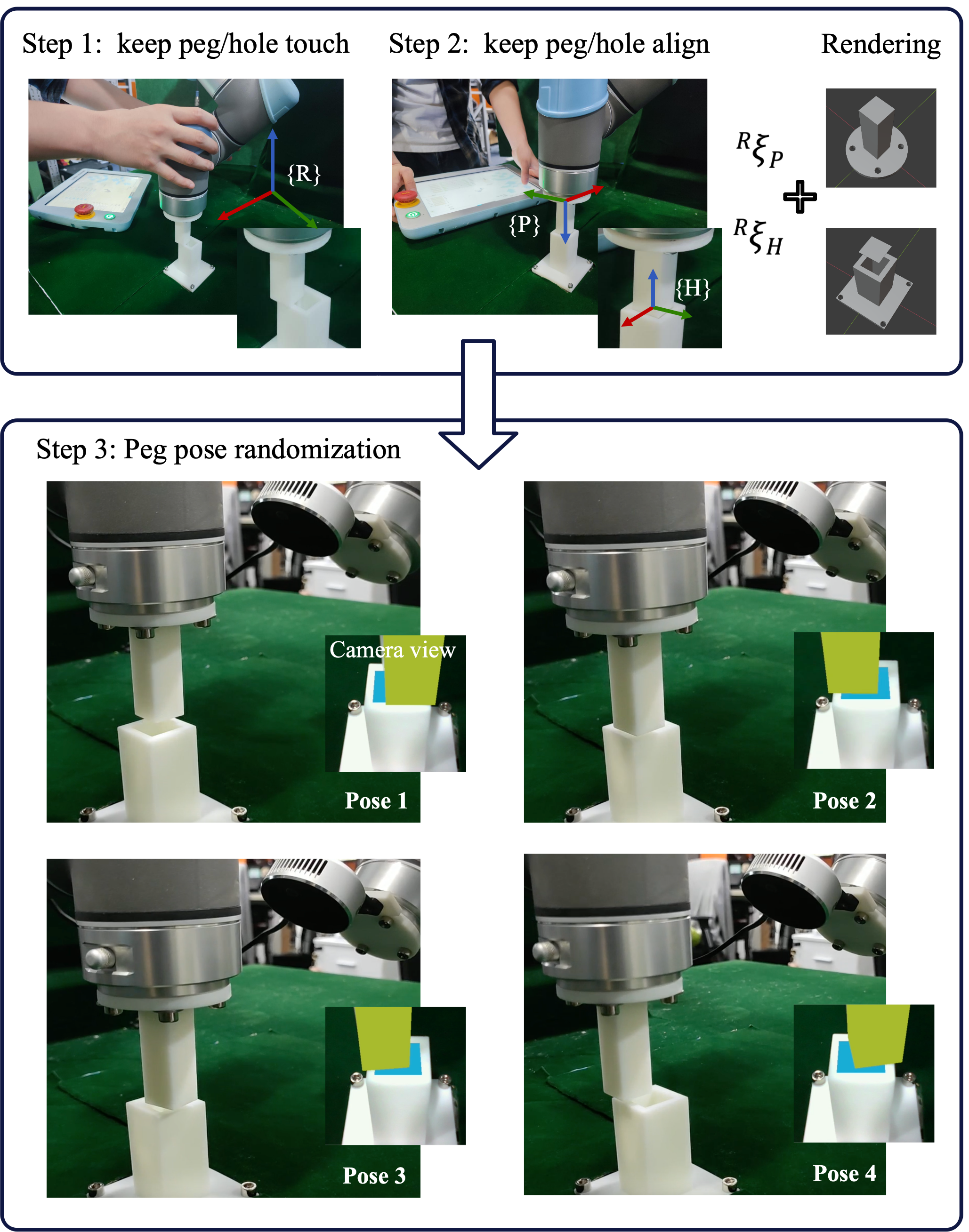
A crucial step of the algorithm presented in the previous section is collecting sufficient real-world training data for the perception adaptation, which would be impractical given the fact that the time-consuming, labor-intensive manual annotation for these data can cost a few days. In this section, we design an automatic data collection and ground truth annotation pipeline for the SN fine-tuning, which helps accelerate the adaption to various real-world insertion tasks.

We define the world frame as $\left\{R\right\}$ by taking the robot base as the origin in the coordinate system. We also define the reference frame as $\left\{P\right\}$ which is attached to the robot end-effector, and the reference frame $\left\{H\right\}$ which indicates the hole pose. The pipeline has three steps as illustrated in Fig. 4. Firstly, the peg is kept in touch with the hole by moving the robot end-effector with a human demonstration. Secondly, by controlling the direction key of the teaching pendant, the peg-hole pose can be aligned precisely. After completing the two steps, the peg/hole poses in the robot coordinate system can be obtained. Concretely, The peg can be regarded as the robot end-effector in the robot-peg system, where the peg pose ${}^{R}\xi_{P}$ can be controlled and calculated by robot kinematics. The hole is fixed in the world space, and the hole pose ${}^{R}\xi_{H}$ can be obtained by robot kinematics with the current joint angles. With the known 3D peg/hole models and known peg/hole poses, the peg/hole masks can be obtained by rendering the 3D models with their poses in Pyrender [43]. Finally, by controlling and randomizing the peg pose relative to the hole, a training dataset consisting of the RGB images, their paired masks, and the corresponding relative poses can be obtained. Notably, the masks are annotated for training the SN and the relative poses can be leveraged for fine-tuning the VSN. The whole process only needs one-minute human teaching to get the hole pose with all the data collection and annotation done by the robot automatically, which is time-efficient and manually cost-minimal.

IV Controller Design

The reference frame axes in P indicates the 6-DoF peg pose, which consists of the end-effector position $\textbf{x}\in\mathbb{R}^{3}$ and the end-effector rotation $\mathbf{R}\in\mathbf{SO}(3)$. The produced actions of the policy are represented in the reference frame $\left\{P\right\}$. Our policy solves the 4-DoF peg-in-hole which consists of the 3-DoF position x and the $z$-axis yaw rotation $\theta$.

Figure 5: Decoupled motion-force controller

TABLE I: Task Coefficients

Coefficient	Value
Position heatmap size ($M$)	21 pixels
Rotation resolution ($\beta$)	2∘
Number of LSTM layers	1
Hidden size of LSTM layer	32
Number of Historical frames ($n$)	5
Maximum trajectory length ($k_{max}$)	100
Discount factor ($\gamma$)	0.995
PD proportional gain ($k_{pm}$)	20
PD differential gain ($k_{vm}$)	5
PI proportional gain ($k_{pf}$)	0.004
PI integral gain ($k_{if}$)	1
Constant contact force ($\mathbf{f}_{\rm d}$)	10N

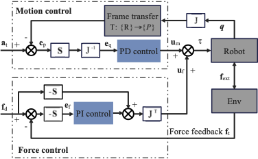
We use the hybrid motion-force controller to execute the end-effector control commands (see Fig. 5). For the motion control, the desired action $\mathbf{a}_{\rm t}$ produced by the policy is executed by a PD controller with the control law defined as:

$$\mathbf{e}_{\rm q}=\mathbf{S}\mathbf{J}^{\rm-1}(\mathbf{a}_{\rm t}-\mathbf{T}_{R}^{P}\mathbf{Jq})$$ (21)

$$\mathbf{u}_{\rm m}=k_{pm}\mathbf{e}_{\rm q}+k_{vm}\mathbf{\dot{e}}_{\rm q}$$ (22)

where S is the diagonal matrix to decouple the motion and force control, J is end-effector Jacobian, T is the transform matrix from $\left\{R\right\}$ to $\left\{P\right\}$, q is joint displacement in joint space, $k_{pm}$ and $k_{vm}$ are proportional gain and differential gain respectively. For the force control, constant contact force $\mathbf{f}_{\rm d}$ between the peg and the hole is expected to be maintained by a PI controller with the control law defined as:

$$\mathbf{e}_{\rm f}=-\mathbf{S}(\mathbf{f}_{\rm d}-\mathbf{f}_{\rm t})$$ (23)

$$\mathbf{u}_{\rm f}=\mathbf{J}^{\rm T}(k_{pf}\mathbf{e}_{\rm f}+k_{if}\int\mathbf{e}_{\rm f}-\mathbf{{S}}\mathbf{f}_{\rm d})$$ (24)

where $\mathbf{f}_{\rm t}$ is the force feedback from the F/T sensor, $k_{pf}$ and $k_{if}$ are the proportional gain and the integral gain respectively.

V Implementations

Figure 6: VSN prediction error under increasing tolerances (0.2$mm$, 0.6$mm$, 1.0$mm$) on (a) $x$-axis with the eye-to-hand configuration (b) $y$-axis with the eye-to-hand configuration (c) $yaw$ rotation with the eye-to-hand configuration (d) $x$-axis with the eye-in-hand configuration (e) $y$-axis with the eye-in-hand configuration (f) $yaw$ rotation with the eye-in-hand configuration.

We build a simulation environment in PyBullet [21] for model training. We use the Franka Panda robot, a 7-DoF torque-controlled robot, of which the end-effector is connected by a peg with a fixed joint. A wrist F/T sensor is mounted to measure the contact force. An RGB camera is either fixed at the world space following [4] (eye-to-hand) or mounted at the robot end-effector[22] (eye-in-hand). In addition, we also evaluate the proposed method on a real-world platform, which consists of a 6-DoF UR5 robot, a Robotiq FT300 wrist F/T sensor, and a calibrated camera of Intel RealSense L515. We use Pyrender, a physically-based Python library, to obtain the segmentation masks by rendering the 3D models.

We use a single Nvidia GeForce GPU (RTX 2070) with an Intel Core (i7 8700) for data collection and model training. For each insertion trajectory, early termination occurs on successful insertion or if the robot end-effector leaves the safe region. We set 50$mm$ for the maximum safe distance. The RGB image resolution is cropped to 224$\times$224.

The initial position error ranges from -10$mm$ to 10$mm$ and the initial rotation error ranges from $-10^{\circ}$ to $10^{\circ}$. To evaluate the shape generalization, 4 seen peg shapes (Fig. 1(b)) are designed for training and 8 unseen peg shapes (Fig. 1(c)) for evaluation. The 8 unseen peg shapes are selected from general daily insert tasks which range from simple to complex, concave to convex, and square-corner to round-corner. More details can be found in Tab. I.

VI Experiments

We design a series of experiments to examine the effectiveness and practicability of the proposed framework. In particular, our goal is to evaluate the generalization ability on the unseen holes and the fast adaptation attributes. Experiments are designed and conducted to answer the following five questions:

• Generalization: Is the policy able to generalize to the objects that are unseen in the training set?

• Efficiency: How fast the vision feedback peg-in-hole can be under 10$mm$ initial error on the unseen shapes?

• Precision: What is the performance trend of the sub-$mm$ peg-in-hole with decreasing tolerances?

• Robustness: Is the policy able to plan a feasible trajectory under vision occlusion with only one camera?

• Adaptation: How fast the proposed system can be adapted from simulation to different unseen real-world scenarios?

Figure 7: Feature visualization of the VSN: raw images(top), segmented images(upper-middle), position feature maps (lower-middle) and rotation feature maps (bottom).

VI-A Simulations

VI-A1 Generalization of the VSN

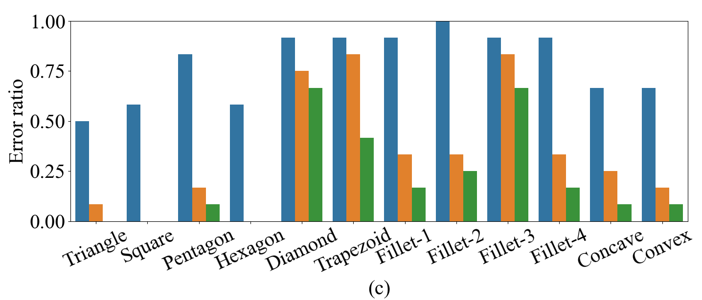
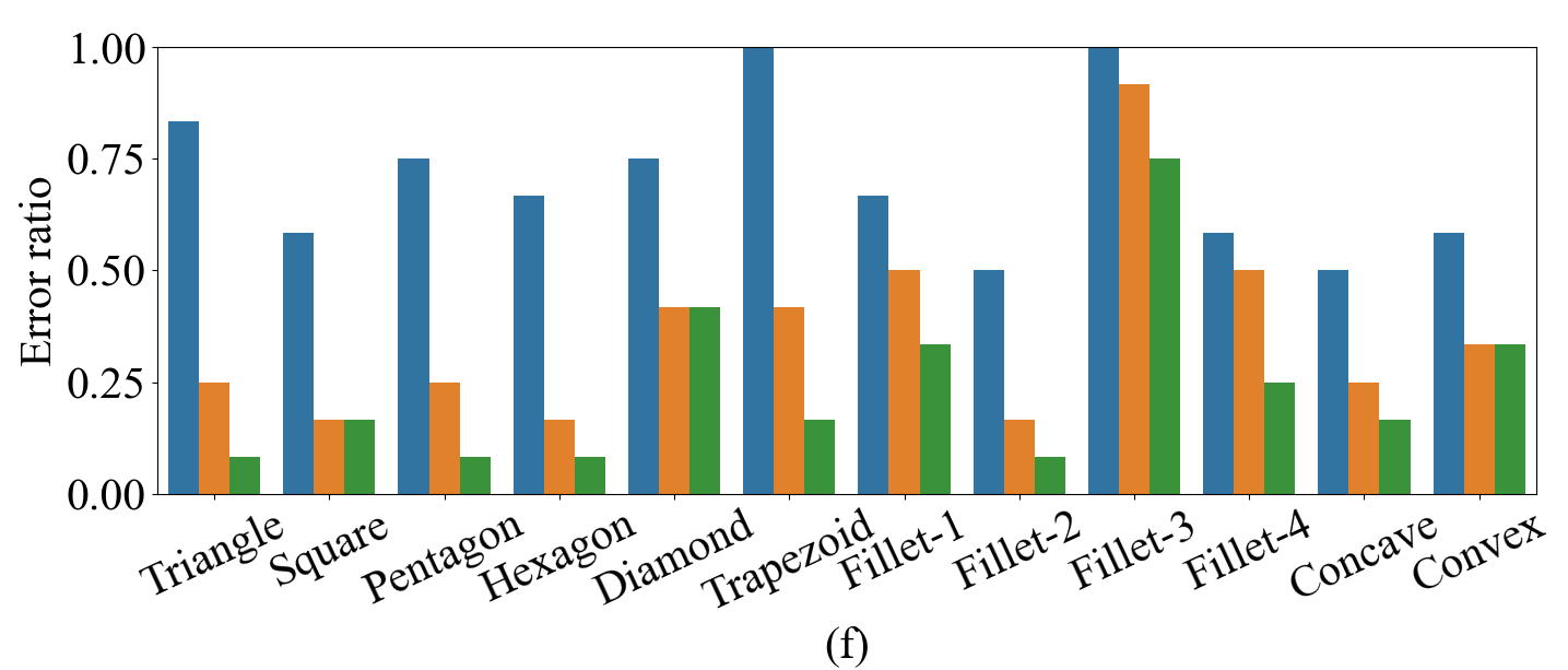
We evaluate the generalization of the VSN by calculating the VSN precision on the seen and unseen holes respectively. The VSN precision is evaluated from three dimensions: $x,y$-axis and $yaw$ rotation respectively, by comparing the predicted value $dx,dy$ and the rotation $d\theta$ with the corresponding ground truth value $v^{*}$ as:

$$Error~{}ratio~{}(v)=\frac{\#\{trials~{}with~{}|v-v^{*}|>tol\}}{\#\{total~{}trials\}}$$ (25)

$$v=dx,~{}dy,~{}or~{}d\theta$$ (26)

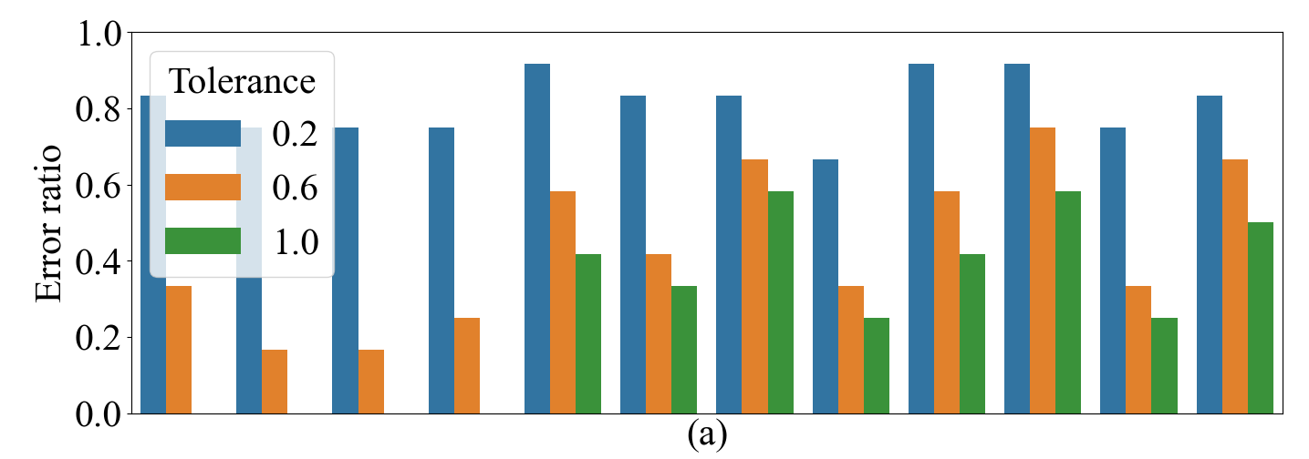
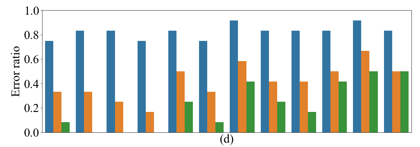
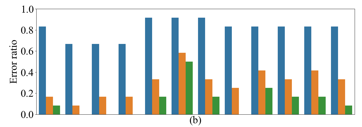
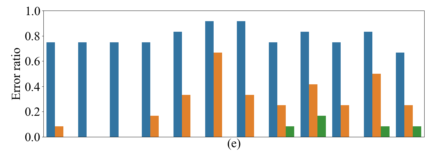
where $\#\{\cdot\}$ means the trial number and $tol$ is the hole tolerance. We evaluate the VSN precision with three different hole tolerances: 0.2$mm$, 0.6$mm$ and 1.0$mm$. The results are the average of 12 random trials for each shape under both the eye-to-hand and the eye-in-hand configurations. As shown in Fig. 6, we observe that the VSN has a high precision on the $y$-axis with the averaged error ratio under 0.2 with 1.0$mm$ tolerance. The VSN performs relatively poorly on the $x$-axis, where the camera is mounted, due to the reason that the prediction on the $x$-axis relies heavily on the accurate mapping from the pixel distance to the real world displacement. However, the VSN still reduces the averaged error ratio to 0.4 with 1.0$mm$ tolerance. We also observe that for the $yaw$ rotation under the eye-to-hand configuration, the peg outline changes as the robot moves, which is harder for the VSN to extract the line/corner features for the rotation alignment, but the VSN achieves a high precision with the error ratio lower than 0.25 for most shapes with 1.0$mm$ tolerance. It is notable that with sub-$mm$ tolerance (0.6$mm$), which is much more challenge than the 1.0$mm$ tolerance setting, the VSN achieves competitive performances on all the three dimensions, particularly under the seen shapes.

VI-A2 Feature Visualization of the VSN

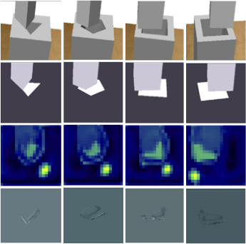
To figure out what has been learned inside the VSN, we perform feature visualization to display the outputs of the VSN. Fig. 7 visualizes the results, where the top row contains the raw images captured from the RGB camera under four different conditions, where the first three columns are three different peg/hole pairs with the same initial pose, and the last two columns share the same peg/hole shape but are initialized with different poses. The upper-middle row is the corresponding segmented images, the lower-middle row are the one-hot heatmaps produced by the position feature extraction module, and the bottom row is the feature maps of the rotation feature extraction module. For the position feature extraction, we can find that the position of the brightest point in the heatmap keeps track of the hole, which indicates that the position module focuses on the relative position between the peg-hole while avoiding over-fitting to the geometry features. For the rotation feature extraction, the feature maps have learned to encode the general features (corner, line features) of the segmented image for rotation alignment. In general, the designed VSN architecture is insensitive to the shape differences but learns to encode general features to determine the relative position and rotation between the peg and the hole, which explains the shape generalization of the proposed VSN.

Figure 8: Sub-$mm$ Insertion performance averaged on (a) seen shapes under eye-to-hand (b) unseen shapes under eye-to-hand (c) seen shapes under eye-in-hand (d) unseen shapes under eye-in-hand configuration.

TABLE II: Insertion Performance with 1$mm$ Tolerance in Simulation

[t] Seen Unseen shape Methods 1 2 3 4 Average 1 2 3 4 5 6 7 8 Average Success rate VSN policy 10/12 12/12 9/12 10/12 85.4% 3/12 1/12 4/12 6/12 2/12 4/12 8/12 6/12 35.4% VSN policy^∗ 9/12 11/12 11/12 10/12 85.4% 5/12 5/12 8/12 8/12 4/12 8/12 8/12 9/12 57.3% E2E vision-RL 12/12 12/12 12/12 12/12 100% 2/12 3/12 $\times$ $\times$ $\times$ $\times$ $\times$ 2/12 7.3% E2E vision-RL^∗ 11/12 12/12 12/12 11/12 95.8% 3/12 5/12 $\times$ $\times$ $\times$ $\times$ $\times$ $\times$ 8.3% Single-frame 12/12 12/12 12/12 12/12 100% 12/12 12/12 12/12 12/12 12/12 11/12 12/12 4/12 92.7% Single-frame^∗ 12/12 12/12 12/12 12/12 100% 12/12 12/12 12/12 12/12 12/12 11/12 9/12 8/12 93.8% Multi-frame 12/12 12/12 12/12 12/12 100% 11/12 12/12 12/12 12/12 11/12 11/12 12/12 6/12 91.7% Multi-frame^∗ 12/12 12/12 12/12 12/12 100% 12/12 12/12 12/12 12/12 12/12 11/12 10/12 9/12 94.8% Insertion efficiency (s) E2E vision-RL 5$\pm$1.6 5$\pm$0.9 5$\pm$1.7 4$\pm$1.2 5$\pm$1.4 12$\pm$2.1 6$\pm$2.0 $\times$ $\times$ $\times$ $\times$ $\times$ 9$\pm$2.1 8$\pm$3.0 E2E vision-RL^∗ 5$\pm$1.6 5$\pm$0.9 5$\pm$1.7 4$\pm$1.3 5$\pm$1.4 9$\pm$4.0 7$\pm$2.2 $\times$ $\times$ $\times$ $\times$ $\times$ $\times$ 8$\pm$3.0 Single-frame 7$\pm$2.5 4$\pm$1.3 5$\pm$1.6 5$\pm$1.6 6$\pm$3.0 9$\pm$3.8 6$\pm$2.3 5$\pm$2.6 5$\pm$2.2 11$\pm$4.4 8$\pm$3.1 7$\pm$3.1 15$\pm$3.4 8$\pm$4.4 Single-frame^∗ 3$\pm$1.4 3$\pm$1.4 3$\pm$1.7 3$\pm$1.9 3$\pm$1.6 7$\pm$5.1 3$\pm$1.8 4$\pm$2.1 3$\pm$1.8 5$\pm$3.1 4$\pm$4.1 4$\pm$4.1 4$\pm$1.4 4$\pm$3.3 Multi-frame 4$\pm$1.0 3$\pm$0.9 3$\pm$0.8 3$\pm$0.8 3$\pm$1.0 4$\pm$1.6 4$\pm$1.2 7$\pm$3.6 4$\pm$0.8 6$\pm$3.0 6$\pm$3.4 7$\pm$3.4 10$\pm$4.7 6$\pm$3.2 Multi-frame^∗ 2$\pm$1.2 3$\pm$1.4 3$\pm$1.0 3$\pm$1.3 3$\pm$1.2 3$\pm$2.5 4$\pm$1.7 4$\pm$4.8 3$\pm$1.6 6$\pm$2.8 4$\pm$2.4 4$\pm$3.4 3$\pm$0.5 4$\pm$3.0

• This superscript denotes the method is not general to the insertion tasks.

• Cases with ^∗ are tested in eye-in-hand configuration, whilst without ^∗ are eye-to-hand configuration.

VI-A3 Peg-in-hole with 0.1$\rm\sim$1mm Tolerance

We compare the proposed policy (VSN+CN) with the following two alternative methods: the VSN (alone) and the E2E Vision-RL [44]. The same 4 seen peg/hole pairs are selected to train the policy and 8 unseen pairs are selected for evaluation.

VSN Policy: Since the VSN has explicitly produced the translation $dx,dy$ in Eq. 4 and the rotation $d\theta$ in Eq. 10, we can perform one-shot insertion by moving the robot-peg to the target pose calculated by $dx,dy,d\theta$.

E2E Vision-RL: Takes the segmented image instead of the raw RGB image as input as with our proposed method for a fair comparison. The policy network, action space, and reward function is defined the same as in [44].

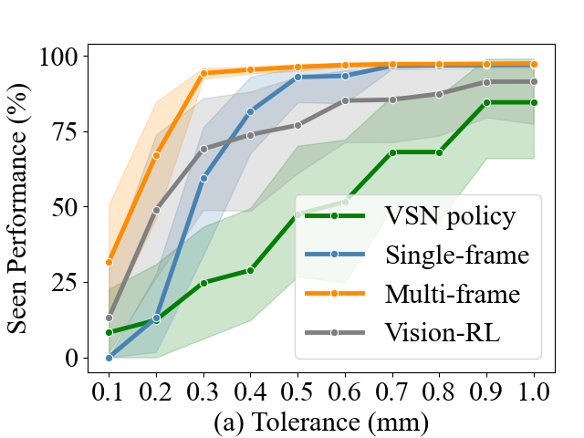
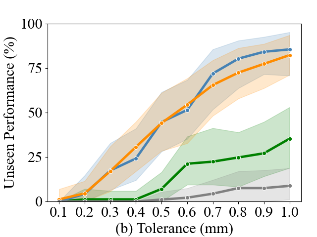
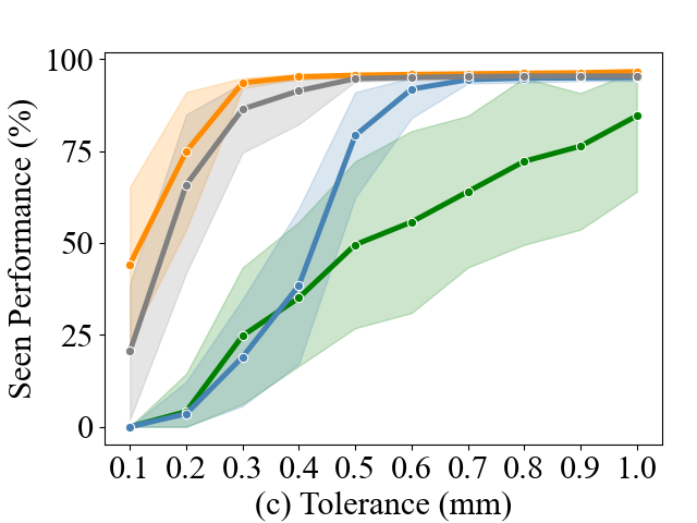
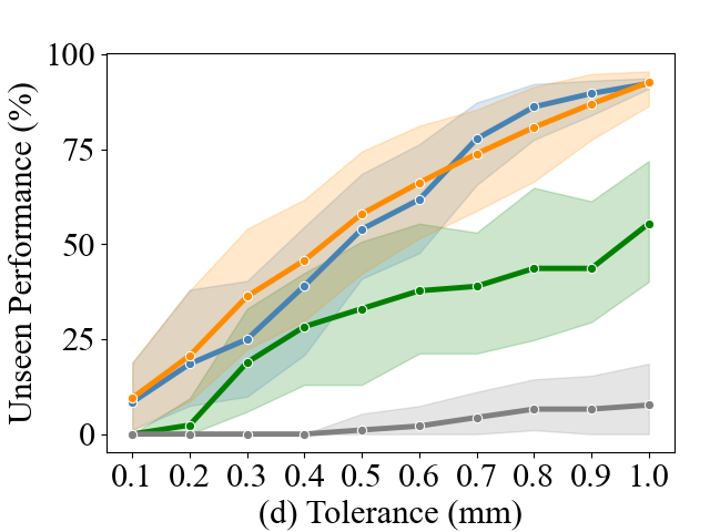
We explore the insertion performance with sub-$mm$ tolerance. The performance is evaluated by counting the total rewards (defined in Eq. 16) of the full insertion trajectory. The reward is designed to encourage the policy to achieve success insertion with minimal steps. Thus the performance reflects both the success rate and insertion efficiency. The hole tolerance ranges from 0.1 to 1$mm$ with 10 steps. Results are averaged over 4 seen and 8 unseen shapes respectively under both the eye-to-hand and eye-in-hand configurations, with each shape performing 12 random insertion trials, which counts to 2880 trials in total. As shown in Fig. 8, the performance curve ascends with the increasing tolerance on both the seen and the unseen shapes and under both the eye-in-hand and the eye-to-hand configurations. However, we find that the E2E Vision-RL performs well on the insertions with the seen shape, while struggling to generalize to the unseen shapes. Compared with the VSN policy, our proposed policies (the single-frame and the multi-frame policy) help promote the insertion performance, though they rely on the VSN to generalize to the unseen shapes. In addition, we find that the performance of the multi-frame policy exceeds that of the single-frame policy on the seen shapes, while their performances are level pegging on the unseen shapes. We assume that the superiority of the multi-frame policy over the single-frame policy is based on the higher precision of the VSN.

Since the performance gap is the largest among the compared methods when the tolerance is 1$mm$ as shown in Fig. 8, we further compare the success rate and insertion efficiency respectively with 1$mm$ hole tolerance. The insertion efficiency is calculated by averaging over the total moving steps of the successful insertion trajectories. Cases that exceed the predefined safe region are regarded as a fail trajectory. The initial position error is 10$mm$ and the rotation error is $10^{\circ}$. The results of each shape are illustrated in Tab. II. We find that our proposed multi-frame and single-frame policies achieve better averaged results on both success rate and insertion efficiency compared with the VSN policy and the E2E Vision-RL. Notably, they outperform the E2E Vision-RL by large margins in terms of success rate on the unseen shapes (>90% vs. <10%). We also find that the multi-frame policy achieves faster insertion with fewer steps compared with the single-frame policy on both the seen and the unseen shapes and under both the eye-in-hand and eye-to-hand configurations. We believe that by considering the historical visual information and actions, the multi-frame policy is aware of the sensor prediction error and forges ahead bravely, while the single-frame policy can only proceed cautiously with small steps by only taking as input the current visual feature with uncertainty.

VI-B Real World Experiments

We use the peg-hole pairs with around 0.6$mm$ tolerance for all the real-world experiments. We design the 3D mesh of the peg-hole pairs in Blender, an open software for 3D modeling, with the clearance between 0.5$mm$ to 0.7$mm$. The 3D print error is 0.2$mm$.

TABLE III: Insertion Performance with 0.6$mm$ Tolerance in Real World

[t] Seen Unseen shape Methods 1 2 3 4 Average 1 2 3 4 5 6 7 8 Average 5mm / Success rate Spiral Search ^† 10/12 11/12 11/12 10/12 87.5% 9/12 9/12 10/12 9/12 8/12 8/12 7/12 7/12 69.7% E2E Force-RL ^† 11/12 10/12 11/12 11/12 89.6% 9/12 9/12 8/12 9/12 8/12 8/12 5/12 5/12 65.3% E2E Vision-RL 12/12 12/12 11/12 11/12 97.9% $\times$ $\times$ $\times$ $\times$ $\times$ $\times$ $\times$ $\times$ $\times$ E2E Vision-RL^∗ 12/12 12/12 11/12 12/12 97.9% $\times$ $\times$ $\times$ $\times$ $\times$ $\times$ $\times$ $\times$ $\times$ Ours 11/12 11/12 10/12 11/12 89.6% 9/12 9/12 8/12 7/12 7/12 7/12 6/12 6/12 61.5% Ours^∗ 11/12 10/12 12/12 11/12 91.75 9/12 10/12 9/12 7/12 7/12 7/12 7/12 7/12 65.6% 5mm / Insertion efficiency (s) Spiral Search ^† 10$\pm$3.1 9$\pm$3.0 8$\pm$2.5 10$\pm$2.8 9$\pm$3.0 10$\pm$3.2 9$\pm$3.4 11$\pm$3.2 10$\pm$3.7 11$\pm$3.5 9$\pm$3.1 11$\pm$3.8 10$\pm$3.3 10$\pm$3.3 E2E Force-RL ^† 4$\pm$1.6 3$\pm$1.1 5$\pm$1.3 3$\pm$2.1 4$\pm$1.7 4$\pm$0.9 5$\pm$1.2 3$\pm$0.9 4$\pm$1.0 3$\pm$1.0 5$\pm$1.1 11$\pm$2.3 6$\pm$1.5 5$\pm$1.8 E2E Vision-RL 5$\pm$0.9 3$\pm$1.1 3$\pm$1.3 4$\pm$1.6 4$\pm$1.2 $\times$ $\times$ $\times$ $\times$ $\times$ $\times$ $\times$ $\times$ $\times$ E2E Vision-RL^∗ 4$\pm$0.8 4$\pm$1.2 3$\pm$0.9 3$\pm$1.1 5$\pm$1.1 $\times$ $\times$ $\times$ $\times$ $\times$ $\times$ $\times$ $\times$ $\times$ Ours 4$\pm$1.5 4$\pm$0.8 5$\pm$1.7 5$\pm$1.2 4$\pm$1.1 3$\pm$1.7 4$\pm$1.5 4$\pm$1.5 5$\pm$2.0 4$\pm$1.5 5$\pm$2.2 6$\pm$1.9 5$\pm$1.4 4$\pm$1.5 Ours^∗ 3$\pm$0.4 4$\pm$0.8 3$\pm$1.3 4$\pm$1.4 3$\pm$1.2 4$\pm$1.5 3$\pm$1.7 3$\pm$0.9 4$\pm$1.5 4$\pm$1.3 4$\pm$1.6 6$\pm$1.5 5$\pm$1.5 4$\pm$1.5 10mm / Success rate Spiral Search ^† 5/12 6/12 5/12 5/12 43.8% 6/12 7/12 6/12 5/12 5/12 4/12 1/12 3/12 36.5% E2E Force-RL ^† $\times$ $\times$ $\times$ $\times$ $\times$ $\times$ $\times$ $\times$ $\times$ $\times$ $\times$ $\times$ $\times$ $\times$ E2E Vision-RL 11/12 12/12 11/12 11/12 93.8% $\times$ $\times$ $\times$ $\times$ $\times$ $\times$ $\times$ $\times$ $\times$ E2E Vision-RL^∗ 10/12 11/12 12/12 11/12 91.7% $\times$ $\times$ $\times$ $\times$ $\times$ $\times$ $\times$ $\times$ $\times$ Ours 11/12 11/12 10/12 10/12 87.5% 7/12 8/12 7/12 6/12 7/12 6/12 6/12 4/12 53.1% Ours^∗ 10/12 11/12 11/12 11/12 89.6% 8/12 8/12 7/12 6/12 6/12 6/12 6/12 4/12 54.3% 10mm / Insertion efficiency (s) Spiral Search ^† 23$\pm$4.5 25$\pm$4.6 21$\pm$3.9 23$\pm$3.6 23$\pm$4.1 22$\pm$4.8 22$\pm$4.4 23$\pm$4.3 24$\pm$4.4 23$\pm$5.1 24$\pm$4.5 25$\pm$3.1 25$\pm$4.5 24$\pm$4.5 E2E Force-RL ^† $\times$ $\times$ $\times$ $\times$ $\times$ $\times$ $\times$ $\times$ $\times$ $\times$ $\times$ $\times$ $\times$ $\times$ E2E Vision-RL 5$\pm$1.3 5$\pm 1.8$ 6$\pm$2.4 4$\pm$1.5 5$\pm$1.6 $\times$ $\times$ $\times$ $\times$ $\times$ $\times$ $\times$ $\times$ $\times$ E2E Vision-RL^∗ 5$\pm$1.2 4$\pm$1.5 5$\pm$1.7 4$\pm$1.2 5$\pm$1.5 $\times$ $\times$ $\times$ $\times$ $\times$ $\times$ $\times$ $\times$ $\times$ Ours 4$\pm$0.9 5$\pm$1.2 6$\pm$1.0 5$\pm$1.6 5$\pm$1.3 5$\pm$1.8 5$\pm$1.2 6$\pm$1.3 5$\pm$1.5 5$\pm$1.5 4$\pm$1.3 6$\pm$2.4 4$\pm$1.7 5$\pm$1.5 Ours^∗ 4$\pm$0.4 5$\pm$1.1 5$\pm$0.8 4$\pm$1.5 4$\pm$1.2 5$\pm$2.0 4$\pm$1.3 4$\pm$1.4 4$\pm$1.7 5$\pm$1.3 4$\pm$0.8 6$\pm$1.9 5$\pm$1.3 5$\pm$1.4

• This superscript denotes the 3-DoF peg-in-hole.

• This superscript denotes the method is not general to the insertion tasks.

• Cases with ^∗ are tested in eye-in-hand configuration, whilst without ^∗ are eye-to-hand configuration.

VI-B1 Peg-in-hole with 0.6mm Tolerance

We compare the proposed multi-frame policy with three previous works on success rate, insertion efficiency (defined in Sec. VI-A3), and unseen shape generalization. The compared alternatives include the previously mentioned E2E Vision-RL and the following two methods.

Spiral Search [8]: Will move downward in the $z$-axis until a force limit is reached, indicating the peg has been in contact with the hole. Then the peg moves outwards in a spiral while pressing against the hole surface. When the peg moves over the hole within a success region, the force in $z$-axis will help press the peg to insert compliantly. Otherwise, the peg will move until exceeding the uncertainty boundary and fail.

E2E Force-RL [5]: Learns the policy end-to-end, which outputs the 2D translate displacement $[dx,dy]$ in the horizon space by taking the 6D force/torque $[F_{x},F_{y},F_{z},M_{x},M_{y},M_{z}]$ as input. Force control is performed in the $z$-axis to maintain a constant contact as with the spiral search. The sparse reward is given when the insert successes within possibly the minimum steps as defined in [5]. The model is trained in simulation and transferred to the real-world directly.

As shown in Tab. III, the force-based methods like spiral search and E2E Force-RL achieve comparable insertion success rate with the vision-based methods when the initial error is within 5$mm$. However, spiral search is inefficient and the success rate drops rapidly with a larger initial error (10$mm$), as the search-based open-loop control method relies heavily on the initial position. For the E2E Force-RL, it fails to be general when the initial error is 10$mm$. We believe that the force/torque distribution gap between the simulation and the real-world grows wider with a larger initial error. And directly policy transfer finds it hard to tolerate the larger gap, which results in poor performance. Moreover, in experiments we found the force-based methods fail to learn the rotation alignment under large yaw error in $z$-axis (10^∘). Due to this reason, we take one step back by performing 3-DoF peg-in-hole that only outputs $dx,dy,dz$ in the action space, which is unfair to the vision-based 4-DoF peg-in-hole that considers the extra $z$-axis rotation error. For the vision-based methods, we find that the E2E Vision-RL achieves both a high success rate and efficiency by over-fitting to the seen shapes during training, but pays for the price for not being general to the unseen shapes. Our proposed multi-frame policy can realize both a higher success rate and efficiency while generalizing to the unseen shapes under both the eye-in-hand and the eye-to-hand configurations.

VI-B2 Perception Adaptation

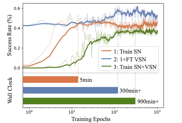
We conduct the perception adaptation to achieve sim-to-real using efficient supervised learning. The training data is collected and annotated in the real-world platform automatically. Three adaptation strategies are compared. The first strategy only trains the SN and keeps the VSN fixed which is pre-trained in simulation. The second one begins with a trained SN and fine-tunes the VSN pre-trained in simulation. The third one trains the SN and the VSN from scratch with real-world data. 500 RGB images with annotations for both the SN and the VSN are collected in around 15 minutes by randomly changing the robot end-effector’s pose relative to the hole without contact. The relative distance ranges from -10 to 10$mm$ in the $x$ and $y$ axis, and the relative $z$-axis yaw rotation ranges from $-10^{\circ}$ to $10^{\circ}$. The 500 images are divided into the training set and the testing set by a ratio of 9:1. Fig. 9 illustrates the success rate of the VSN policy on the testing set. We can find that the performance curve of the first strategy converges fast ( $\sim$10 training epochs) in around 5 minutes, which achieves 0.97 $MeanIoU$[45] with nearly perfect segmentation precision and around 0.45 success rate. The success rate of the second strategy outperforms the first one by up to 10%. Significant improvement of the VSN is achieved by fine-tuning the VSN with real-world data, though at the cost of around 5 hours’ training. The curve of the third strategy converges until 300 epochs, which takes around 15 hours for training. The final performance of the third strategy does not exceed that of the first strategy, which we believe is because of the lack of real-world data for training the VSN from scratch. In real-world experiments, we adopt the first strategy for fast perception adaptation.

VI-B3 Robustness under Vision Occlusion

We evaluate the robustness of the proposed system when the vision occlusion occurs with the Fillet-1 shape (see Fig. 1). Fig. 10 shows the perspective of the camera, where the hole is occluded entirely by the peg in the initial state. Under the vision occlusion, the VSN policy loses the reference to align the peg pose relative to the hole, thus drifting off the safe zone where no historical or future information can provide the reference for the policy to pull back and fails to align the peg-hole pose. However, both the multi-frame and single-frame policy can recover from the vision blind with the help of the CN, but the multi-frame policy recovers faster than the single-frame policy. We infer that the prediction uncertainty from the VSN is reduced by considering the historical sensor features and actions, which contributes to the convergence of the multi-frame policy.

Figure 9: Success rate of the VSN policy with three different adaptation strategies.

VI-C EV Charging

Finally, we conduct the real-world experiments in the automatic EV charging system, which is a complete unseen insertion scenario, to evaluate the practicability of our proposed algorithms. We achieve fast perception adaptation on the platform within 20 minutes, including automatic data collection, annotation, and segmentation training. The policy is trained with the same four seen shapes in simulation as mentioned above and developed in the vehicle charging case directly without fine-tuning. The initial position and rotation error is within 10$mm$ and $10^{\circ}$ respectively.

VI-C1 Static Insertion

The experiment platform is built with the Tesla Model 3, the UR5e robot arm, the RealSense D435 camera, the charging plug, and the LED flash as shown in Fig. 11(a). The camera is fixed at the robot’s wrist with the eye-in-hand configuration. The policy starts by commanding the robot to approach the hole, and touch the surface with constant contact based on force signals from the build-in F/T sensor. Then the pose alignment is achieved by the proposed algorithm. Finally, when the aligning process finishes, the peg will be pushed into the hole compliantly under the constant force to realize the insertion. We count a 10/10 success rate under random initial poses, with each insertion completed within 3s, which verifies the practicability of the proposed system.

VI-C2 Dynamic Insertion

We further evaluate the proposed framework in more challenging conditions. The agent needs to perform a dynamic insertion while a person is manually moving the EV socket (see Fig. 11(b)). This is much harder than the static insertions. Results show that our methods can solve these very challenging tasks effectively. More insertion cases can be found in the supplemented videos [46].

VI-D Discussion

Through the simulations and real-world experiments, we answer the previously mentioned five questions on generalization, efficiency, precision, robustness, and adaptation for peg-in-hole, and discuss the strengths and potentials of our proposed framework.

• The experiments examine the effectiveness and practicability of our proposed framework across various peg insertion tasks. Evaluation of a series of hole shapes demonstrates the simulation-based generic policy can apply to a wide variety of unseen insertion tasks, which proves that the policy is trained with several shapes, and tested to another set of shapes unseen in the training set.

• Our approach achieves efficient insertion under large initial error (10$mm$ and 10^∘) in around 3s, which is much faster than the force-based methods. The error range almost covers the initial error caused by the upstream tasks such as object pose estimation, mobile robot navigation, etc. However, theoretically, by enlarging the measurement range or resolution of the VSN, our method can scale up to a broader error range as long as the hole is in the visual field.

  

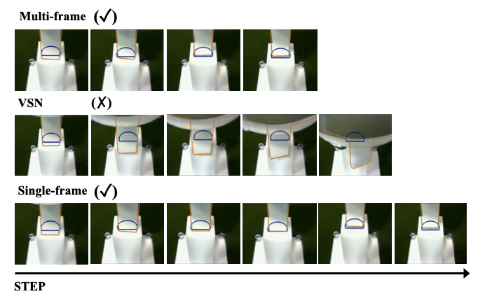
  Figure 10: Peg-hole pose aligning trajectory under camera view: the multi-frame policy performs fast and accurate pose alignment; the VSN policy drifts away from the safe zone; the single-frame policy can achieve pose alignment but is inefficient.

• Experiments in both simulation and real-world prove that under 1$mm$ hole tolerance, our approach achieves a high success rate (> 90%) and insertion efficiency on both the seen and unseen holes, and it performs well in the dynamic insertion scenario, which is a more challenge task. We further explore the performance of our approach with 0.6$mm$ tolerance in the real world. The insertion success rate remains $\sim$ 90% with tighter tolerances on the seen holes, while achieving > 50% success rate on the unseen holes, which is consistent with the simulated results. To improve the performance on the unseen holes under sub-$mm$ tolerance, we can use extra task-specific data to fine-tune the VSN structure. We prove more than 10% improvement in the success rate can be achieved for the VSN with extra training. We do not quantify the improvement for the peg-in-hole by fine-tuning the VSN in the real-world experiments, as a follow-up force-based method can be combined to cover the performance gap if sub-$mm$ precision is required.

  

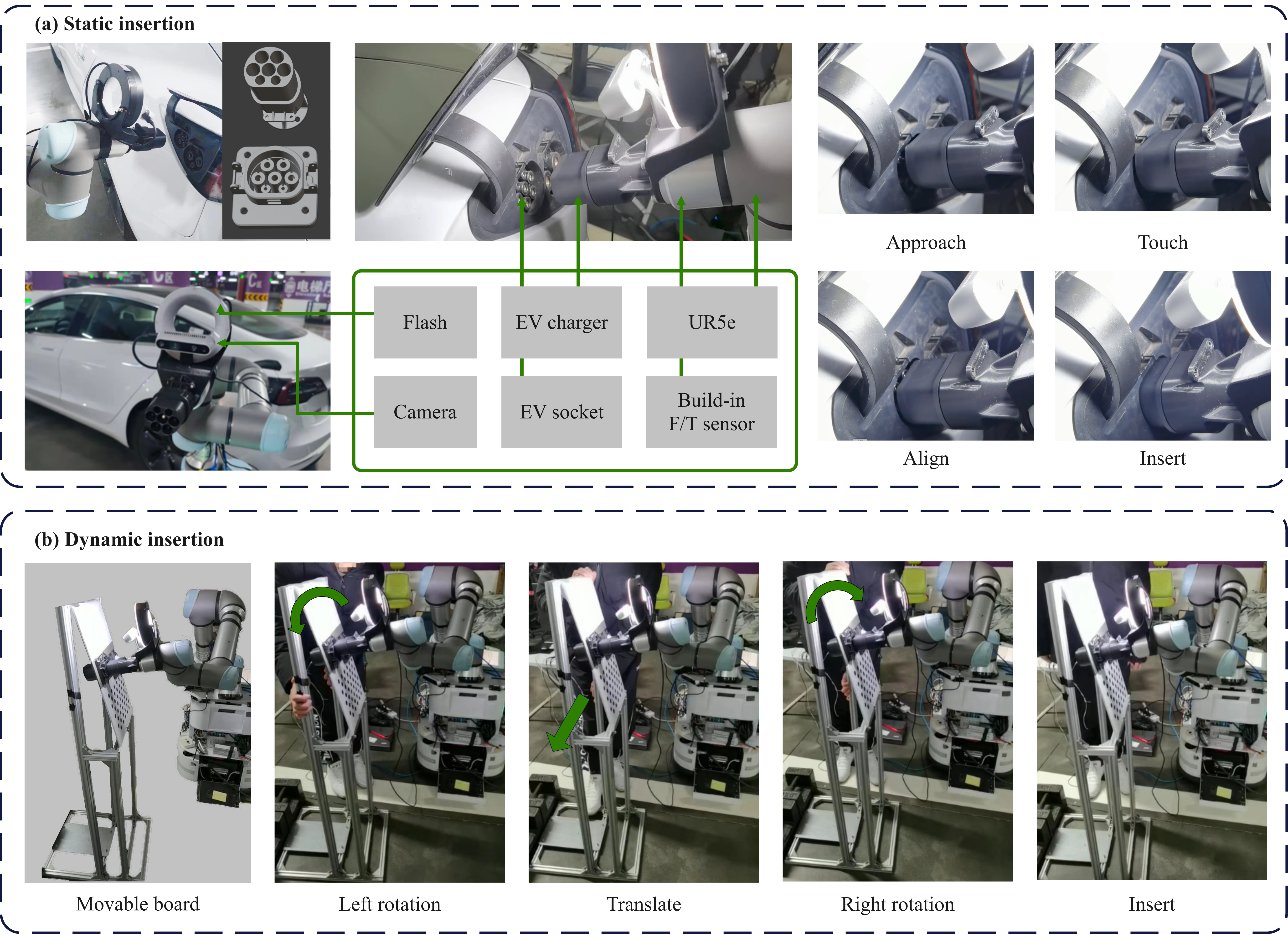
  Figure 11: Real-world plugging of the EV charging system. (a) Static insertion in a real car of Tesla Model 3. (b) Dynamic insertion with the EV socket mounted to a movable board.

• Under vision occlusion circumstances where the hole is totally occluded, the VSN policy faces the ambiguity problem as a given visual state can correspond to multiple pose initialization. Thus the VSN policy fails to align the peg-hole pose when the vision occlusion occurs. The proposed single-frame and multi-frame policy solve the ambiguity by considering future or historical information with the CN module. And the multi-frame policy proves to be more efficient for peg insertion tasks in the real-world experiments. Notably, the multi-frame policy tasks as input the image sequence, thus occupying more graphics memory than the single-frame policy. In lightweight applications where computing resources are limited, the single-frame policy can be a competitive alternative method.

• By fine-tuning the SN, our framework can adapt to various real-world insertion tasks with only hundreds of images in 20 minutes, including data collection, annotation, and model training. The adaptation only needs one-minute human teaching with an accurate insertion to achieve automatic data collection and annotation, without the requirement of expert programming. Similar to the traditional position control for peg insertion, which calls for an accurate insertion by a human to achieve the repetitive positioning, our method requires the same minimal additional cost.

• While our framework presents a step toward generalizable peg insertion, the generalization of visual perception remains a great challenge, especially in the dynamic and unstructured outdoor environments. Combining the current domain randomization techniques with our proposed automatic data collection and annotation pipeline to acquire a huge diversity of data would be a promising direction for future research.

VII Conclusion

In the peg insertion tasks, vision feedback control is preferred compared with other input modalities (e.g. force, tactile, senseless, etc.), especially under large initial error. However, current vision-based solutions for peg-in-hole show poor performance to new objects with unseen shape. In this article, we present a vision feedback framework for precise peg-in-hole towards unseen shape generalization. Our framework enables training a generic insertion policy with several shapes in simulation, and adapting to arbitrary unseen shapes in real-world with minimal sim-to-real cost. The cost contains a fast perception adaptation process, which calls for one-minute manual teaching to bootstrap the automatic data collection and annotation pipeline. With the fast adaptable-adaptation module, the simulation-based generic policy can quickly generalize to various real-world insertion tasks, either under the eye-to-hand or eye-in-hand configuration. In the future work, we plan to pursue the tight insertion tasks for higher precision and robustness by combining the vision and force/torque data and extend to the 6-DoF insertion tasks. We also want to explore the use of new progress in computer vision fields, such as domain randomization, to achieve perception generalization.

Liang Xie received the B.Eng. in electrical and information engineering from Hunan University, Changsha, China, in 2017. He is currently working toward the Ph.D. degree at the State Key Laboratory of Industrial Control Technology and Institute of Cyber-Systems and Control, Zhejiang University, Hangzhou, China. His research interests include precision assembly, robot manipulation, and robot learning.

Hongxiang Yu received the B.Eng. degree in Control Science and Engineering from Zhejiang University, Hangzhou, China, in 2017. He is currently pursuing the Ph.D. degree at the State Key Laboratory of Industrial Control Technology and Institute of Cyber-Systems and Control, Zhejiang University, Hangzhou, China. His current research interests include grasping, visual servoing, and robot learning.

Kechun Xu received her B.Eng. in Control Science and Engineering from Zhejiang University, Hangzhou, China, in 2021. She is currently working toward Ph.D degree at the State Key Laboratory of Industrial Control Technology and Institute of Cyber-Systems and Control, Zhejiang University, Hangzhou, China. Her research interests include robot manipulation and robot learning.

Tong Yang (Student Member, IEEE) received the B.Eng. degree from the Department of Control Science and Engineering, Zhejiang University, Hangzhou, China, in 2018, where he is currently working toward the Ph.D degree with the Robotic Laboratory. His current research interests include robot planning and control.

Minhang Wang received his M.S. from the Department of Electronic Engineering, Xidian University, Xi’an, P.R. China in 2013. He is currently a Senior engineer in Application Innovate Laboratory, Huawei Technologies Co., Beijing, China. His main research interests include lifelong SLAM and robotic vision.

Haojian Lu (Member, IEEE) received B.Eng. degree in Mechatronical Engineering from Beijing Institute of Technology in 2015, and he received Ph.D degree in Robotics from City University of Hong Kong in 2019. He was a Research Assistant at City University of Hong Kong, from 2019 to 2020. He is currently a professor in the State Key Laboratory of Industrial Control and Technology, and Institute of Cyber-Systems and Control, Zhejiang University. His research interests include micro/nanorobotics, bioinspired robotics, medical robotics, micro aerial vehicle and soft robotics.

Yue Wang (Member, IEEE) received the Ph.D degree from the Department of Control Science and Engineering, Zhejiang University, Hangzhou, China, in 2016. He is currently working as an Associate Professor with the Department of Control Science and Engineering, Zhejiang University. His current research interests include mobile robotics and robot perception.

Rong Xiong (Member, IEEE) received the Ph.D degree from the Department of Control Science and Engineering, Zhejiang University, Hangzhou, China, in 2009. She is currently a professor with the Department of Control Science and Engineering, Zhejiang University. Her current research interests include motion planning and SLAM.

References

- [1] J. Xu, Z. Hou, Z. Liu, and H. Qiao, “Compare contact model-based control and contact model-free learning: A survey of robotic peg-in-hole assembly strategies,” 2019.
- [2] T. Z. Zhao, J. Luo, O. Sushkov, R. Pevceviciute, N. Heess, J. Scholz, S. Schaal, and S. Levine, “Offline meta-reinforcement learning for industrial insertion,” 2021.
- [3] J. Luo, O. Sushkov, R. Pevceviciute, W. Lian, and J. Scholz, “Robust multi-modal policies for industrial assembly via reinforcement learning and demonstrations: A large-scale study,” 2021.
- [4] R. L. Haugaard, J. Langaa, C. Sloth, and A. G. Buch, “Fast robust peg-in-hole insertion with continuous visual servoing,” arXiv preprint arXiv:2011.06399, 2020.
- [5] T. Inoue, G. De Magistris, A. Munawar, T. Yokoya, and R. Tachibana, “Deep reinforcement learning for high precision assembly tasks,” in 2017 IEEE/RSJ International Conference on Intelligent Robots and Systems (IROS). IEEE, 2017, pp. 819–825.
- [6] M. A. Lee, Y. Zhu, K. Srinivasan, P. Shah, S. Savarese, L. Fei-Fei, A. Garg, and J. Bohg, “Making sense of vision and touch: Self-supervised learning of multimodal representations for contact-rich tasks,” in 2019 International Conference on Robotics and Automation (ICRA). IEEE, 2019, pp. 8943–8950.
- [7] L. Xie, H. Yu, Y. Zhao, H. Zhang, Z. Zhou, M. Wang, Y. Wang, and R. Xiong, “Learning to fill the seam by vision: Sub-millimeter peg-in-hole on unseen shapes in real world,” 2022. [Online]. Available: https://arxiv.org/abs/2204.07776
- [8] J. A. Marvel, R. Bostelman, and J. Falco, “Multi-robot assembly strategies and metrics,” ACM Computing Surveys, vol. 51, no. 1, pp. 1–32, 2018.
- [9] Y. Fei and X. Zhao, “An assembly process modeling and analysis for robotic multiple peg-in-hole,” Journal of Intelligent and Robotic Systems, vol. 36, no. 2, pp. 175–189, 2003.
- [10] Zhang, Kuangen, Jing, Chen, Heping, Zhao, Jianguo, and Ken, “Jamming analysis and force control for flexible dual peg-in-hole assembly,” IEEE Transactions on Industrial Electronics, vol. 66, no. 3, pp. 1930–1939, 2019.
- [11] A. S. Morgan, B. Wen, J. Liang, A. Boularias, A. M. Dollar, and K. Bekris, “Vision-driven compliant manipulation for reliable, high-precision assembly tasks,” arXiv preprint arXiv:2106.14070, 2021.
- [12] R. Blake, K. V. Sobel, and T. W. James, “Neural synergy between kinetic vision and touch,” Psychol, vol. 15, no. 6, pp. 397–402, 2010.
- [13] S. Levine, N. Wagener, and P. Abbeel, “Learning contact-rich manipulation skills with guided policy search,” 2015. [Online]. Available: https://arxiv.org/abs/1501.05611
- [14] X. Zhang, S. Jin, C. Wang, X. Zhu, and M. Tomizuka, “Learning insertion primitives with discrete-continuous hybrid action space for robotic assembly tasks,” 2021. [Online]. Available: https://arxiv.org/abs/2110.12618
- [15] E. Y. Puang, K. P. Tee, and W. Jing, “KOVIS: Keypoint-based visual servoing with zero-shot sim-to-real transfer for robotics manipulation,” in 2020 IEEE/RSJ International Conference on Intelligent Robots and Systems (IROS). IEEE, oct 2020. [Online]. Available: https://doi.org/10.1109%2Firos45743.2020.9341370
- [16] Y. Zhu, Z. Wang, J. Merel, A. Rusu, T. Erez, S. Cabi, S. Tunyasuvunakool, J. Kramár, R. Hadsell, N. de Freitas, and N. Heess, “Reinforcement and imitation learning for diverse visuomotor skills,” 2018. [Online]. Available: https://arxiv.org/abs/1802.09564
- [17] Y. Zhu, Z. Wang, J. Merel, A. Rusu, and N. Heess, “Reinforcement and imitation learning for diverse visuomotor skills,” 2018.
- [18] G. Schoettler, A. Nair, J. A. Ojea, S. Levine, and E. Solowjow, “Meta-reinforcement learning for robotic industrial insertion tasks,” 2020.
- [19] S. Levine, N. Wagener, and P. Abbeel, “Learning contact-rich manipulation skills with guided policy search,” Proceedings IEEE International Conference on Robotics and Automation, 2015.
- [20] G. Thomas, M. Chien, A. Tamar, J. A. Ojea, and P. Abbeel, “Learning robotic assembly from cad,” pp. 1–9, 2018.
- [21] B. H. Cristian, D. Petit, I. G. Ramirez-Alpizar, and K. Harada, “Variable compliance control for robotic peg-in-hole assembly: A deep reinforcement learning approach,” Applied Sciences, vol. 2020, no. 10, p. 6923, 2020.
- [22] J. C. Triyonoputro, W. Wan, and K. Harada, “Quickly inserting pegs into uncertain holes using multi-view images and deep network trained on synthetic data,” in 2019 IEEE/RSJ International Conference on Intelligent Robots and Systems (IROS). IEEE, 2019, pp. 5792–5799.
- [23] S. P. Arunachalam, S. Silwal, B. Evans, and L. Pinto, “Dexterous imitation made easy: A learning-based framework for efficient dexterous manipulation,” 2022. [Online]. Available: https://arxiv.org/abs/2203.13251
- [24] S. Endrawis, G. Leibovich, G. Jacob, G. Novik, and A. Tamar, “Efficient self-supervised data collection for offline robot learning,” 2021. [Online]. Available: https://arxiv.org/abs/2105.04607
- [25] K. Zakka, A. Zeng, J. Lee, and S. Song, “Form2fit: Learning shape priors for generalizable assembly from disassembly,” in 2020 IEEE International Conference on Robotics and Automation (ICRA). IEEE, 2020, pp. 9404–9410.
- [26] J. A. Bagnell, “Reinforcement learning in robotics: A survey,” 2014.
- [27] T. Tang, H.-C. Lin, Y. Zhao, Y. Fan, W. Chen, and M. Tomizuka, “Teach industrial robots peg-hole-insertion by human demonstration,” in 2016 IEEE International Conference on Advanced Intelligent Mechatronics (AIM), 2016, pp. 488–494.
- [28] M. Andrychowicz, B. Baker, M. Chociej, R. Jozefowicz, B. Mcgrew, J. Pachocki, A. Petron, M. Plappert, G. Powell, and A. Ray, “Learning dexterous in-hand manipulation,” 2018.
- [29] X. B. Peng, M. Andrychowicz, W. Zaremba, and P. Abbeel, “Sim-to-real transfer of robotic control with dynamics randomization,” 2017.
- [30] K. Bousmalis, A. Irpan, P. Wohlhart, Y. Bai, M. Kelcey, M. Kalakrishnan, L. Downs, J. Ibarz, P. Pastor, and K. Konolige, “Using simulation and domain adaptation to improve efficiency of deep robotic grasping,” IEEE, 2018.
- [31] A. Hämäläinen, K. Arndt, A. Ghadirzadeh, and V. Kyrki, “Affordance learning for end-to-end visuomotor robot control,” 2019. [Online]. Available: https://arxiv.org/abs/1903.04053
- [32] J. Tobin, R. Fong, A. Ray, J. Schneider, W. Zaremba, and P. Abbeel, “Domain randomization for transferring deep neural networks from simulation to the real world,” 2017.
- [33] S. Stevšić, S. Christen, and O. Hilliges, “Learning to assemble: Estimating 6d poses for robotic object-object manipulation,” IEEE Robotics and Automation Letters, vol. 5, no. 2, pp. 1159–1166, 2020.
- [34] J. Ding, C. Wang, and C. Lu, “Transferable force-torque dynamics model for peg-in-hole task,” arXiv preprint arXiv:1912.00260, 2019.
- [35] J. Ruiz-del Solar, P. Loncomilla, and N. Soto, “A survey on deep learning methods for robot vision,” 2018. [Online]. Available: https://arxiv.org/abs/1803.10862
- [36] S. Dong, D. K. Jha, D. Romeres, S. Kim, D. Nikovski, and A. Rodriguez, “Tactile-rl for insertion: Generalization to objects of unknown geometry,” arXiv preprint arXiv:2104.01167, 2021.
- [37] K. Hsu, M. J. Kim, R. Rafailov, J. Wu, and C. Finn, “Vision-based manipulators need to also see from their hands,” 2022. [Online]. Available: https://arxiv.org/abs/2203.12677
- [38] A. Nibali, Z. He, S. Morgan, and L. Prendergast, “Numerical coordinate regression with convolutional neural networks,” 2018.
- [39] O. Ronneberger, P. Fischer, and T. Brox, “U-net: Convolutional networks for biomedical image segmentation,” 2015. [Online]. Available: https://arxiv.org/abs/1505.04597
- [40] ROOPAK, SHAH, EDUARD, SCKINGER, JAMES, W., BENTZ, ISABELLE, GUYON, and C. and, “Signature verification using a ”siamese” time delay neural network,” International Journal of Pattern Recognition and Artificial Intelligence, vol. 07, no. 4, pp. 669–669, 1993.
- [41] D. P. Vassileios Balntas, Edgar Riba and K. Mikolajczyk, “Learning local feature descriptors with triplets and shallow convolutional neural networks,” in Proceedings of the British Machine Vision Conference (BMVC), E. R. H. Richard C. Wilson and W. A. P. Smith, Eds. BMVA Press, September 2016, pp. 119.1–119.11. [Online]. Available: https://dx.doi.org/10.5244/C.30.119
- [42] V. Mnih, A. P. Badia, M. Mirza, A. Graves, T. Lillicrap, T. Harley, D. Silver, and K. Kavukcuoglu, “Asynchronous methods for deep reinforcement learning,” in International conference on machine learning. PMLR, 2016, pp. 1928–1937.
- [43] M. Matl, “Pyrender,” https://github.com/mmatl/pyrender, 2019.
- [44] G. Schoettler, A. Nair, J. Luo, S. Bahl, J. A. Ojea, E. Solowjow, and S. Levine, “Deep reinforcement learning for industrial insertion tasks with visual inputs and natural rewards,” in 2020 IEEE/RSJ International Conference on Intelligent Robots and Systems (IROS). IEEE, 2020, pp. 5548–5555.
- [45] J. Long, E. Shelhamer, and T. Darrell, “Fully convolutional networks for semantic segmentation,” 2015.
- [46] L. Xie, “Learning visual guided policy for precision peg-in-hole with unseen shape generalization,” 2022. [Online]. Available: https://github.com/xieliang555/SFN.git
![[Uncaptioned image]](/html/2205.04297/assets/images/xiel.png) |