Bell inequalities for nonlocality depth

Abstract

When three or more particles are considered, quantum correlations can be stronger than the correlations generated by so-called hybrid local hidden variable models, where some of the particles are considered as a single block inside which communication and signaling is allowed. We provide an exhaustive classification of Bell inequalities to characterize various hybrid scenarios in four- and five-particle systems. In quantum mechanics, these inequalities provide device-independent witnesses for the entanglement depth. In addition, we construct a family of inequalities to detect a non-locality depth of $(n-1)$ in $n$-particle systems. Moreover, we present two generalizations of the original Svetlichny inequality, which was the first Bell inequality designed for hybrid models. Our results are based on the cone-projection technique, which can be used to completely characterize Bell inequalities under affine constraints; even for many parties, measurements, and outcomes.

I Introduction

Bell inequalities have been successfully used to show that the results of Bell test experiments are incompatible with local hidden-variable (LHV) models Brunner et al. (2014); Shalm et al. (2015); Giustina et al. (2015); Hensen et al. (2015); Rosenfeld et al. (2017). Moreover, nonlocality has been linked to communication complexity problems Buhrman et al. (2010) and Bell inequalities have been found useful for device independent verification of quantum states and measurements Šupić and Bowles (2020).

Given the phenomenon of quantum nonlocality, one may ask whether for three or more particles novel effects occur. To answer this question, George Svetlichny introduced in 1987 so-called hybrid models Svetlichny (1987). Hybrid models are a class of hidden variable models that give up on all restrictions on the correlations between a subset of parties while maintaining the restriction of local realism with respect to the remaining ones. The most famous example of a hybrid model is the one originally introduced by Svetlichny for three parties: In any round of the Bell experiment, two of the parties may collaborate to establish arbitrary correlations between themselves (see also Fig. 1). However, the correlations shared between these two parties and the third party must respect a LHV model. In this case, the correlations between the three parties satisfy the Svetlichny inequality Svetlichny (1987), which reads

$$\langle A_{1}B_{1}C_{2}\rangle+\langle A_{1}B_{2}C_{1}\rangle+\langle A_{2}B_{1}C_{1}\rangle-\langle A_{2}B_{2}C_{2}\rangle$$

$$+\langle A_{2}B_{2}C_{1}\rangle+\langle A_{2}B_{1}C_{2}\rangle+\langle A_{2}B_{1}C_{1}\rangle-\langle A_{1}B_{1}C_{1}\rangle \leq 4,$$ (1)

where $A_{a},B_{b},C_{c}$ denote measurements on parties A, B, and C, respectively, and each of the measurements yields outcomes $\pm 1$. In quantum mechanics, the Svetlichny inequality is maximally violated up to a value of $4\sqrt{2}$ by the Greenberger-Horne-Zeilinger (GHZ) state

$$|\text{GHZ}\rangle=\frac{1}{\sqrt{2}}(|000\rangle+|111\rangle).$$ (2)

the Svetlichny inequality has been generalized to more particles Collins et al. (2002a), and experimental violations of these inequalities have also been observed Lavoie et al. (2009); Zhao et al. (2003).

(a)

(b)

(c)

Figure 1: Illustration of different hybrid models. (a) In the scenario considered by Svetlichny, in each round of the Bell experiment two of the three parties (here, Alice and Bob) form a team and are allowed to communicate. In (b) and (c) we see two different hybrid models for four parties. In each round of the experiment, there could be two teams of two parties each (b) or one team of three parties and an isolated party (c). The behaviors that can arise from scenario (b) form a so-called $(2,2)$ model, scenario (c) gives rise to a $(3,1)$ model.

For our further discussion it will be convenient to have a compact notation. By defining $[abc]:=\langle A_{a}B_{b}C_{c}\rangle$, we can write the Svetlichny inequality as

$$4 -[112]-[121]-[211]+[222]$$

$$-[221]-[212]-[122]+[111]\geq 0.$$ (3)

We have mentioned before that a violation of the Svetlichny inequality implies genuine tripartity nonlocality that cannot be explained by a hybrid model. Let us shortly explain why this is the case. Assume that Alice and Bob can share arbitrary correlations, since the inequality is symmetric under exchange of parties this is no restriction of generality. Allowing arbitrary correlations among two parties amounts to treating both together as one party. Rewriting the Svetlichny inequality in this way yields

$$4-[12]-[21]-[31]+[42]-[41]-[32]-[22]+[11]\geq 0.$$ (4)

This inequality, however, can be written as the sum of two Clauser-Horne-Shimony-Holt (CHSH) inequalities Clauser et al. (1969, 1970),

$$2-[12]-[21]-[22]+[11]\geq 0,$$ (5)

$$2-[31]+[42]-[41]-[32]\geq 0.$$ (6)

Consequently, for models which are local with respect to the $AB|C$ partition, the Svetlichny inequality holds, and violation of it requires at least one of the two CHSH inequalities Eq. (5), Eq. (6) to be violated. Due to the permutation symmetry of the Svetlichny inequality this argument shows that a violation of the Svetlichny inequality implies that any two parties share nonlocality with the remaining one.

As mentioned earlier, the Svetlichny inequality is violated in quantum mechanics, which means that nonlocality affects more than two particles at once. To gain a better understanding of this phenomenon, it is desirable to find other inequalities for hybrid scenarios. In the scenario considered by Svetlichny, there is only one full-body correlation hybrid inequality, which is different from the Svetlichny inequality, found by Jean Daniel Bancal et al. Bancal et al. (2010). Moreover, hybrid Bell inequalities have been derived for an arbitrary number of parties Collins et al. (2002a), an arbitrary number of parties with two dichotomic measurements Bancal et al. (2011) and also scenarios with $n$ parties that have access to $m$ measurements with $o$ outcomes each Bancal et al. (2012). Beyond this, scenarios have been considered in which some parties are grouped together, but within such as group still all correlations in the hidden-variable models obey the nonsignaling constraint Almeida et al. (2010).

The question arises, how one can find Bell inequalities for hybrid models of four and five parties. For more than three parties there is more than one hybrid model to consider (see Fig. 1). For four parties, one example of a hybrid model would be one, where two teams of two parties share local correlations while the correlations shared between parties within a team can be arbitrary. In the following we refer to this hybrid model as a $(2,2)$ model. Another example would be a hybrid model where there is one team of three parties and one party that is on its own. In our terminology, this is a $(3,1)$ model.

In this paper, we consider all hybrid models for four and five parties and find all optimal, symmetric, full-body correlation Bell inequalities, for two settings with two outcomes per observer. Full-body correlation Bell inequalities are those that only involve correlations where every party performs a non-trivial measurement. Such inequalities have been considered in detail for the usual notion of fully local hidden variable models Żukowski and Brukner (2002); Werner and Wolf (2001). Requiring symmetry of the Bell inequalities imposes linear contraints, which can be incorporated using the cone-projection technique (CPT) Bernards and Gühne (2020, 2021). This technique helps to reduce the dimensionality of the problem and thus simplifies the task and allows us to find all Bell inequalities. Finally, we then shift our focus back to three-partite nonlocality, where we discuss genuine-multipartite Bell inequalities with three settings that generalize the Svetlichny inequality. This means that for a particular choices of measurements, these inequalities reduce to the Svetlichny inequality. Again, the CPT allows to tackle this problem.

II Hybrid models

Consider a Bell experiment where the parties perform local measurements that yield outcomes $\pm 1$. The parties can then describe the behavior of the experiment by estimating the expectation values for all combinations of measurements, such as $\langle A_{a}B_{b}C_{c}\rangle$. Such an expectation value is called a correlation. A behavior is a vector that encodes the information of some or all of the correlations measured in the experiment. Let $d$ be the number of correlations that are measured in the experiment. Then, the euclidian space $\mathbb{R}^{d}$ can be used to describe all the information encoded in the behaviours. A physical model, such as quantum mechanics, an LHV model or a hybrid model is a subset of the vector space of behaviors. Moreover, every model is a subset of the hypercube defined by the conditions

$$-1\leq\langle A_{a}B_{b}C_{c}\rangle\leq 1.$$ (7)

We refer to this hypercube as the unconstrained model $M_{\square}$. Hybrid models are models that are more restrictive than the unconstrained model but less restrictive than LHV models Svetlichny (1987); Collins et al. (2002b). For the set of hybrid models $M_{H}$ it thus holds that

$$M_{LHV}\subset M_{H}\subset M_{\square},$$ (8)

where $M_{LHV}$ is the set of LHV model and $M_{\square}$ is the set of unconstrained behaviors.

Hybrid models can be constructed in the following way: Given an $n$-party system with subsystems $s\in S$, the first step is to define a partition

$$P =\{c_{1},\ldots,c_{k}\}$$ (9)

where the cells $c_{i}\subset S$ are disjoint and non-empty subsets of $S$ and $\bigcup_{i=1}^{k}c_{i}=S$.

In a second step, one defines a LHV model $M_{LHV}^{P}$ for the coarse grained scenario defined by $P$. This works in the following way: Every cell $c_{i}$ of the partition is considered as one system. The measurement settings are all combinations of measurement settings that apply to each subsystem within a cell. However, no restrictions apply to the correlations between subsystems within a cell, since the cell is regarded as one system. In particular, this allows for signaling to take place between the parties within one cell.

As a third step, two partitions are considered equivalent, if they are related by a relabeling of the parties. Each equivalence class of partitions of a partition $P$ is then defined by what we call the cardinality tuple

$$h_{P}=(|c_{i}|\mid i\in\{1,\ldots,k\},\,c_{i}\in P),$$ (10)

which contains the ordered cardinalities of the cells of $P$. Two partitions $P,P^{\prime}$ are equivalent if and only if $h_{P}=h_{P^{\prime}}$. For any ordered tuple $h$, one defines a hybrid model

$$M_{h}=\text{conv}\Big{(}\bigcup_{P\mid h_{P}=h}M_{LHV}^{P}\Big{)},$$ (11)

where conv denotes the convex hull. Note that $M_{h}$ is a convex polytope, the extremal points of which are the union of the extremal points of models $M_{LHV}^{P}$.

If $h$ is an $m$-tuple, we call $M_{h}$ an $m$-local model and if $m$ is equal to the number of parties, we call the resulting model fully local. A more detailed discussion on different notions of multipartite nonlocality can be found in Refs. Szalay (2019); Baccari et al. (2019). Some authors have for example considered hybrid models that impose a no-signaling constraint on the behaviors of each cell in a given partition Almeida et al. (2010); Bancal et al. (2013). In this setup, device independent certification of entanglement has been investigated Liang et al. (2015); Aloy et al. (2019); Lin et al. (2019); Tura et al. (2019). For four parties and $h_{P}=(2,2)$ all Bell-inequalities that are symmetric under party permutations have been found Curchod et al. (2014). Moreover, it is known, that for full-body correlation Bell inequalities, the additional no-signaling constraint on the parties within each cell does not make a difference Curchod et al. (2015).

Note that there are also other approaches to nonlocality, including the so-called operational approach Gallego et al. (2012). Recently, genuine multipartite nonlocality and entanglement have also been studied in networks. This leads to definitions that are different from genuine multipartite nonlocality as introduced by Svetlichny Navascués et al. (2020); Hansenne et al. (2022); Tavakoli et al. (2022).

III Hybrid Bell inequalities

III.1 Statement of the problem

We consider the case of four and five parties that seek to perform a Bell experiment in order to investigate the structure of the nonlocality they might share. Every party can choose between two measurement settings, each of which yields outcomes $\pm 1$. More specifically, we consider the case in which every party performs one of the two measurements in every round, that is, every party performs a non-trivial measurement in every round. As far as Bell inequalities are concerned, this means that we only consider full-body correlation Bell inequalities. It is worth mentioning that for fully local models, all full-body correlation inequalities are known Werner and Wolf (2001); Żukowski and Brukner (2002). Further, we only consider Bell inequalities that are symmetric under relabeling of the parties. This symmetry constraint is a linear constraint on the coefficients of the Bell inequality in question, so we can employ the cone-projection technique Bernards and Gühne (2021) to specifically find these Bell inequalities.

In order to be able to investigate the nonlocal structure, we need to consider different hybrid models. In the four-party case, these hybrid models are given by the cardinality tuples

$$h\in\{(1,1,1,1),(2,1,1),(2,2),(3,1)\},$$ (12)

where $h=(1,1,1,1)$ corresponds to the fully local model. In the case of five parties, we consider six models given by the cardinality tuples

$$h\in\{ (1,1,1,1,1),(2,1,1,1),(2,2,1),$$ (13)

$$(3,1,1),(3,2),(4,1)\}.$$ (14)

For every model, we find all optimal, symmetric, full-body correlation Bell inequalities.

To aid readability, we introduce some notation that simplifies writing down Bell inequalities which are symmetric under permutation of the parties. For example, for four parties $A,B,C,D$ we write

$$(1122) =\langle A_{1}B_{1}C_{2}D_{2}\rangle+\text{party permutations},$$ (15)

where ’party permutations’ only includes permutations that yield different terms. Therefore, expression Eq. (15) consists of six terms. To give another example,

$$(1112) =\langle A_{1}B_{1}C_{1}D_{2}\rangle+\langle A_{1}B_{1}C_{2}D_{1}\rangle$$

$$\quad+\langle A_{1}B_{2}C_{1}D_{1}\rangle+\langle A_{2}B_{1}C_{1}D_{1}\rangle.$$ (16)

For five parties, the notation works analogously.

III.2 Description of the method

We find the Bell inequalities using the cone-projection technique (CPT), which is introduced and and in detail described in Refs. Bernards and Gühne (2020, 2021). The CPT is a method to completely characterize facet-defining Bell inequalities that obey a set of affine equality constraints. Naively, one may achieve this by simply enumerating all facet-defining Bell inequalities and select those which meet the criteria in a second step. However, the CPT provides is a more elegant and efficient to achieve this goal that even works in cases in which finding all Bell inequalities is infeasible.

The CPT consists of three steps. In the first step, on disregards the normalization and associates a ray with every extremal behavior (that is, a point in the space of all behaviours). Conversely, the extremal behaviors can be recovered from the rays by intersecting with a hyperplane. These rays generate a cone $C$. In the second step, the constraints on the Bell inequalities define a lower-dimensional subspace, into which $C$ is projected. This yields a cone $\widetilde{C}$. In the third step, one finds all Bell inequalities that meet the constraints by enumerating the facet-defining inequalities of $\widetilde{C}$ and checking which of these indeed correspond to facets of $C$. These inequalities are exactly the facet defining Bell inequalities that obey the constraints.

III.3 Numerical analysis of the Bell inequalities

For each Bell inequality, we perform the same numerical analysis. We find a lower bound on the quantum violation using qubit and qutrit systems and an upper bound using the third level of the NPA-hierarchy Navascués et al. (2007, 2008). We also find the no-signaling bound. This is a linear program, which can be solved using, for example, the MOSEK solver noa . We find that while not all inequalities are violated in quantum mechanics, all can be violated using no-signaling behaviors. We calculate the quantum violation of each Bell inequality using a seesaw algorithm that optimizes the settings of one party in every step and cycles through the parties. This algorithm is not guaranteed to yield the maximal quantum violation. However, comparing with the upper bound provided by the NPA-hierarchy, we can confirm that the optimum was achieved (within numerical accuracy) in all cases. All of bounds for the inequalities are listed together with the inequalities in the Supplementary Material, see also the description in Appendix A.

Additionally, we find lower bounds on the noise robustnesses of the inequalities using the states

$$\varrho_{4}(p) =(1-p)|\text{GHZ}_{4}\rangle\langle GHZ_{4}|+\frac{p}{16}\mathds{1}$$ (17)

and for five qubits

$$\varrho_{5}(p) =(1-p)|\text{GHZ}_{5}\rangle\langle GHZ_{5}|+\frac{p}{32}\mathds{1},$$ (18)

where the respective GHZ states are given by

$$|\text{GHZ}_{4}\rangle =\frac{1}{\sqrt{2}}(|0000\rangle+|1111\rangle),$$ (19)

$$|\text{GHZ}_{5}\rangle =\frac{1}{\sqrt{2}}(|00000\rangle+|11111\rangle).$$ (20)

We identify regimes of the parameter $p$, for which some of the hybrid models can be excluded, details are described in Appendix B.

III.4 Four-party nonlocality

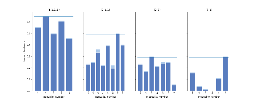
Figure 2: Noise robustness for each inequality for hybrid models in the four-party case, labeled by the respective model. Details can be found in the Supplementary Material A, B, C, and D. Given the family of states $\varrho_{4}(p)$ as defined in Eq. (17) the dark-blue (dark-gray) bar indicates a value of $p$ for which the violation is larger than some threshold (here: $10^{-6}$), the light-blue (light-gray) bar indicates a value of $p$ for which the threshold is no longer exceeded. Note that inequality 4 in the $(3,1)$ model is not violated in quantum mechanics at all. In each plot, the horizontal bar indicates the highest achieved noise robustness.

model	#ineq.	noise-robustness	ineq. number	inequality
(1,1,1,1)	5	0.645	2	$+4-(1111)-(1112)+(1122)+(1222)-(2222)$
(2,1,1)	8	0.493	7	$+4-(1112)+(1222)$
(2,2)	7	0.291	3	$+16-(1112)-2(1122)+3(1222)+4(2222)$
(3,1)	6	0.291	6	$+8+(1111)-(1112)-(1122)+(1222)+(2222)$

Table 1: For each hybrid model, the table shows the number of optimal symmetric full-body correlation inequalities. Further a lower bound for the white-noise robustness for the $|GHZ\rangle$ state is provided for the best inequality, which is labeled by its number in the list in the Supplementary Material.

In the four-party case, we find in total 26 Bell inequalities, five for the fully local model, eight for the $(2,1,1)$ model, seven for the $(2,2)$ model, and six for the $(3,1)$ model. Of these inequalities, we find all but one to be violated in quantum mechanics. All inequalities that are violated in quantum mechanics, are maximally violated by the GHZ state.

For the fully local model, the inequality that exhibits the best white-noise robustness with respect to the GHZ-state is the generalized Mermin inequality

$$+4-(1111)-(1112)+(1122)+(1222)-(2222)\geq 0,$$ (21)

which was already found in Ref. Collins et al. (2002b). With it, nonlocality can be detected with up to roughly $64.5\%$ white noise.

One might expect that for the hybrid models considered, one would find that the Bell inequality with the best noise robustness is a generalized Svetlichny inequality. However, this is not the case. For the $(2,1,1)$ model, the most noise robust Bell inequality is

$$4-(1112)+(1222)\geq 0$$ (22)

and it is violated up to roughly $49.3\%$ of white noise.

If the amount of white noise is less than roughly $p=29.1\%$, then the state $\varrho_{4}(p)$ violates the inequality

$$+8+(1111)-(1112)-(1122)+(1222)+(2222)\geq 0$$ (23)

for the $(3,1)$ model and the inequality

$$+16-(1112)-2(1122)+3(1222)+4(2222)\geq 0$$ (24)

for the $(2,2)$ model. Interestingly, the amount of white-noise required to obtain a violation of the $(2,2)$ model and the $(3,1)$ model is the same for symmetric, full-body correlation, two-setting inequalities, although the violations are established by different inequalities. We will observe the same phenomenon in the case of five parties. The findings discussed in this subsection are summarized in Table 1. The noise robustnesses of all inequalities we found in the four-party case are plotted in Figure 2.

III.5 Five-party nonlocality

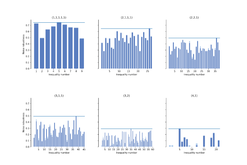
Figure 3: Noise robustness for each inequality for hybrid models in the five-party case, labeled by the respective model. Details can be found in the Supplementary Material E, F, G, H, I, and J. The dark-blue (dark-gray) bar indicates a value of $p$ for which the violation is larger than some threshhold (here: $10^{-6}$), the light-blue (light-gray) bar indicates a value of $p$ for which the threshhold is no longer exceeded. Note that inequalities 30 and 31 of the 3-2 model as well as inequalities 3, 4, 10, 11, 13, 14, 16, 17 and 20 for the 4-1 local model are not violated in quantum mechanics.

model	#ineq.	noise-robustness	ineq. number	inequality
(1,1,1,1,1)	9	0.743	5	$+4-(11112)+(11222)-(22222)$
(2,1,1,1)	27	0.645	26	+8 $+(11111)+(11112)-(11122)-(11222)+(12222)+(22222)$
(2,2,1)	38	0.493	36	$+8+(11111)-(11122)+(12222)$
(3,1,1)	45	0.493	38	$+8+(11111)-(11122)+(12222)$
(3,2)	59	0.291	35	$+40+(11112)+2(11122)-3(11222)-4(12222)+5(22222)$
(4,1)	21	0.291	5	$+16-(11111)+(11112)+(11122)-(11222)-(12222)+(22222)$

Table 2: For each hybrid model, the table shows the number of optimal symmetric full-body correlation inequalities. Further a lower bound for the white-noise robustness for the $|GHZ\rangle$ state is provided for the best inequality, which is labeled by its number in the list in the Supplementary Material.

In the five-party scenario, we find nine inequalities for the fully local model, $27$ inequalities for the $(2,1,1,1)$ model, $38$ inequalities for the $(2,2,1)$ model, $45$ inequalities for the $(3,1,1)$ model, $59$ inequalities for the $(3,2)$ model and $21$ inequalities for the $(4,1)$ model. Among the Bell inequalities in the $(3,2)$ model there are two Bell inequalities that are not violated in quantum mechanics. For the $(4,1)$ model, there are nine such Bell inequalities. All inequalities that are violated are maximally violated in quantum mechanics by the GHZ state.

The Bell inequality for the fully local model with the best white-noise robustness regarding the GHZ state is obtained for the four-party Mermin inequality Collins et al. (2002b)

$$+4-(11112)+(11222)-(22222)\geq 0.$$ (25)

If the percentage of white noise in the state $\varrho_{5}(p)$ is roughly smaller than $74.3\%$, then the state exhibits nonlocality.

For the $(2,1,1,1)$ model, the most sensitive Bell inequality is the four-party Svetlichny inequality Collins et al. (2002b)

$$+8 +(11111)+(11112)-(11122)$$

$$-(22222)+(12222)+(11222)\geq 0.$$ (26)

It can detect a violation up to a white noise level up to roughly $64.5\%$. Note that this is up to numerical precision the same threshold that we obtain for a violation of the fully local model in the case of four parties.

We find numerically that the white-noise thresholds for two-local models, three-local models and five-local models of the four-party scenario and the five-party scenario coincide. For the three-local models given by $h=(2,2,1)$ and $h=(3,1,1)$, we find that the best inequality to detect the nonlocality of a noisy GHZ state is the generalized Mermin inequality Eq. (25), however with a different bound of eight instead of four in the fully local model. It can detect a violation up to approximately $49.3\%$ of white noise.

The two-local models with $h=(3,2)$ and $h=(4,1)$ are violated up to approximately $29.1\%$ of white noise. In the case of the $(4,1)$ model, the violation is detected by the generalized Svetlichny inequality Eq. (26) with an adapted bound of $16$. For the $(3,2)$ model, we find that the most robust Bell inequality is

$$+40+(11112) +2(11122)-3(11222)$$

$$-4(12222)+5(22222)\geq 0.$$ (27)

III.6 Family of hybrid Bell inequalities for many parties

The inequalities Eq. (24) and Eq. (27) which are useful for ruling out a $(2,2)$ model or a $(3,2)$ model, respectively, can be extended to a family of Bell inequalities $(F_{n})$ for an arbitrary number of $n$ parties. We define this family as

$$F_{n}=\sum_{\ell=1}^{n}(-1)^{1+\lceil\frac{\ell}{2}\rceil}\,\ell\,(\underbrace{1\ldots 1}_{n-\ell},\underbrace{2\ldots 2}_{\ell})\leq n2^{n-2}.$$ (28)

One can show that the bound can always be achieved in any $(k,m)$ model with $k,m>1$. Moreover, for $m=2$, one can show analytically that the bound holds. Proofs for both statements can be found in Appendix C. Moreover, we checked numerically for up to $20$ parties that the bound holds for $(k,m)$ models with $k>1,m>1$. We conjecture that the bound also tight for more parties. For $(n-1,1)$ models the bound does not hold. A violation of an inequality in the family Eq. (28) therefore certifies that the nonlocality depth is at least $(n-1)$.

In the following, we discuss numerical findings concerning the Bell inequalities $F_{n}$ for $n\leq 8$ parties. We find, that the quantum bound of the inequalities is

$$F_{n}=\sqrt{2}\,n2^{n-2}$$ (29)

up to numerical precision, which is achieved by choosing $A_{1}=B_{1}=...=\sigma_{x}$ and $A_{2}=B_{2}=...=\sigma_{z}$, where $\sigma_{x},\sigma_{z}$ are Pauli matrices. The quantum states for which a maximal violation can be obtained using these settings are listed in Appendix D. We find numerically that they are equivalent to the GHZ state up to local unitary transformations.

Further, we consider the white-noise robustness. For this, we consider the states

$$\varrho_{n}(p)=(1-p)|\text{GHZ}_{n}\rangle\langle\text{GHZ}_{n}|+p\frac{\mathds{1}_{n}}{2^{n}}.$$ (30)

We find that the inequalities are violated if $p\leq 1-1/{\sqrt{2}}\approx 29.3\%$ up to numerical precision.

IV Generalizations of a Bell inequality to more settings

IV.1 What is a generalization of a Bell inequality?

In this section we explain generalizations of Bell inequalities and present two generalizations of the Svetlichny inequality. Consider a Bell scenario $S_{1}$ and a Bell inequality $\mathbf{b}_{1}$ that is applicable to the scenario $S_{1}$. Additionally, consider a second scenario, $S_{2}$, that is larger than $S_{1}$ in the sense that it involves more parties, more measurement settings per party or more outcomes per measurement setting than $S_{1}$. Let $\mathbf{b}_{2}$ be a Bell inequality for $S_{2}$. Consider the situation in which the parties perform a Bell test for the Bell inequality $\mathbf{b}_{2}$. However, in the number of parties involved in the Bell test and the number and kind of measurements they are allowed to perform, they restrict themselves to the rules given by scenario $S_{1}$. If in this case the Bell test effectively reduces to a Bell test of Bell inequality $\mathbf{b}_{1}$, then we call $\mathbf{b}_{2}$ a generalization of $\mathbf{b}_{1}$.

In Ref. Bernards and Gühne (2020), we introduced and discussed this concept in the case of a generalization to more parties and describe a method how to find generalizations of a given Bell inequality. The concept is best explained by example. Consider three parties, $A,B,C$ that perform a test of Mermin’s inequality

$$+A_{1}B_{1}C_{2}+A_{1}B_{2}C_{1}+A_{2}B_{1}C_{1}-A_{2}B_{2}C_{2}\leq 2.$$ (31)

However, they restrict themselves to the resources of the CHSH scenario. This means that one of the parties is no longer allowed to contribute to the Bell test in a meaningful way. Let this party be $C$. If $C$ reports the measurement outcome $+1$ in every round, then evaluating Mermins inequality effectively means evaluating the inequality

$$+A_{1}B_{1}+A_{1}B_{2}+A_{2}B_{1}-A_{2}B_{2}\leq 2,$$ (32)

which is the well-known CHSH inequality. Therefore, we call Mermin’s inequality a generalization of the CHSH inequality. To be precise, we call an inequality $\mathbf{b}_{2}$ a generalization of an inequality $\mathbf{b}_{1}$ to more parties, if one can make a choice of trivial measurements for the additional parties, such that $\mathbf{b}_{2}$ reduces to $\mathbf{b}_{1}$. By trivial measurement, we mean a measurement that yields one measurement result deterministically. This has as a consequence, that each $(n+1)$-party correlation can be computed from one $n$-party correlation, such as

$$\langle A_{1}B_{2}C_{1}\rangle=\langle A_{1}B_{2}\rangle,$$ (33)

if $C_{1}$ is set to always yield outcome $+1$.

We now turn to an example that illustrates the generalization to a scenario with more settings. Consider the $(3,3;2,2)$ scenario, that is the bipartite scenario, in which every party has three measurement settings and every setting yields outcomes $\pm 1$. Besides the CHSH inequality, there is only one non-trivial facet-defining inequality for this scenario, the I3322 inequality Froissart (1981); Pitowsky and Svozil (2001); Collins and Gisin (2004); Śliwa (2003). This inequality reads

$$A_{1}B_{3}+A_{2}B_{3}+A_{3}B_{1}+A_{3}B_{2}+A_{1}-A_{2}+B_{1}-B_{2}$$

$$-A_{1}B_{1}+A_{1}B_{2}+A_{2}B_{1}-A_{2}B_{2}\leq 4.$$ (34)

As was noted by Collins and Gisin Collins and Gisin (2004), this inequality is strictly stronger than the CHSH inequality with regard to its ability to detect non-locality: If the measurements $A_{3}$ and $B_{1}$ are chosen trivially, so they always yield the result $+1$, then the I3322 inequality reduces to a variant of the CHSH inequality. Therefore the I3322 inequality is a generalization of the CHSH inequality. This example also illustrates an important feature of generalized Bell inequalities: A generalization of a Bell inequality always performs at least as well as the Bell inequality itself in detecting nonlocality for a given quantum state.

In the example of the I3322 inequality, $A$ and $B$ choose one of their measurements trivial to comply with the CHSH scenario. In general, however, this is not the only way to achieve this. Alternatively, the parties may have set two of their measurements equal up to a permutation of outcome labels. When looking for generalizations of a Bell inequality to a scenario with more settings, one must therefore take this possibility into account.

We shall now briefly discuss how to find generalizations of a Bell inequality $\mathbf{b}_{1}$. Let $\mathbf{b}_{1}$ be a Bell inequality for scenario $S_{1}$ and one aims at finding a Bell inequality $\mathbf{b}_{2}$ for a larger scenario $S_{2}$, such that $\mathbf{b}_{2}$ generalizes $\mathbf{b}_{1}$. As a first step, we set the measurement settings that are present in $S_{2}$ additionally to the ones present in $S_{1}$. As discussed earlier, the additional measurement settings are either chosen trivial or equal to other measurement settings of the same party up to outcome label permutations. For each behavior $\beta_{1}$ obtained in scenario $S_{1}$, there is now a behavior $\beta_{2}$ for scenario $S_{2}$ that corresponds uniquely to $\beta_{1}$, in the same fashion as in Eq. (33). We call behavior $\beta_{2}$ the extended behavior of $\beta_{1}$.

The construction of extended behaviors allows us to express the property that $\mathbf{b}_{2}$ is a generalization of $\mathbf{b}_{1}$ as a series of affine constraints: Let $\beta_{1}$ be a behavior that saturates $\mathbf{b}_{1}$. By this we mean that the behavior reaches the maximal classical value of one, which can also be written as a scalar product $\langle\beta_{1},b_{1}\rangle=1$. Then, the extended behavior $\beta_{2}$ must saturate any generalization $\mathbf{b}_{2}$, that is $\langle\beta_{2},b_{2}\rangle=1$. Since the set of all saturating behaviors of $\mathbf{b}_{1}$ defines the inequality $\mathbf{b}_{1}$ in a unique manner, the conditions formulated in this way are not only necessary but also sufficient. This means that if all extended behaviours obey $\langle\beta_{2},b_{2}\rangle=1$, the $\mathbf{b}_{2}$ is a generalization of $\mathbf{b}_{1}$.

So, facet defining inequalities of a polytope that obey a set of affine constraints can be found also using the CPT Bernards and Gühne (2020, 2021). Alternatively, if one is interested in finding the generalizing Bell inequality that is best suited to detect the nonlocality in a given behavior $r$, this is a linear program. One maximizes the expectation value over all inequalities $\mathbf{b}_{2}$ under two constraints. First, the inequality $\mathbf{b}_{2}$ has to obey $\langle\beta_{2},b_{2}\rangle=1$ on all extened behaviours, as explained above. Second, $\mathbf{b}_{2}$ must be a valid Bell-type inequality for all classical behaviours $\beta$ in the considered model of locality, i.e., $\langle\beta,b_{2}\rangle$. More formally, this can be written as:

$$\max_{\mathbf{b}_{2}}\langle r,\mathbf{b}_{2}\rangle$$

s.t. $$\langle\beta_{2},\mathbf{b}_{2}\rangle=1\;\forall\text{ extended saturating behaviors }\beta_{2},$$

$$\langle\beta,\mathbf{b}_{2}\rangle\leq 1\;\forall\text{ extremal behaviors }\beta\text{ of the model}.$$ (35)

Such a linear program can directly be solved using standard numerical techniques.

IV.2 Generalizations of the Svetlichny inequality to more settings

Running the linear program Eq. (35) with random directions $r$, we find two generalizations of the Svetlichny inequality that are symmetric under party permutations for the three-party scenario with three settings per party, or $(3,3,3;2,2,2)$ for short,

$$f_{1}= (100)-(111)+(211)+(221)-(222)$$

$$+2(300)-(310)+(330)+(331)\leq 13$$ (36)

$$f_{2}= -(122)+(123)+(133)-3(222)$$

$$-2(223)+(233)\leq 12.$$ (37)

The inequality $f_{1}$ reduces to the Svetlichny inequality, if one sets $A_{3}=B_{3}=C_{3}=1$. The second inequality, $f_{2}$, reduces to the Svetlichny inequality, if one sets $A_{3}=A_{1},B_{3}=B_{1},C_{3}=C_{1}$.

By construction, the inequalities $f_{1},f_{2}$ are at least as sensitive to nonlocality as the Svetlichny inequality. Moreover, since they have one more setting, one might expect that there might be an advantage of $f_{1}$ and $f_{2}$ compared to the Svetlichny inequality. Unfortunately, sampling 540 random pure three-qutrit states, we did not find a single example that shows an advantage. Rather, we find that choosing the additional settings such that the inequalities reduce to the Svetlichny inequality is always optimal. Accordingly, $f_{1},f_{2}$ share the maximally violating state, the GHZ state, and their noise-robustness with the Svetlichny inequality.

V Conclusion

We presented the complete set of Bell inequalities to rule out various hybrid models for four- and five-body systems. These inequalities can be used to characterize the nonlocality depth in these systems. Our analysis of GHZ states mixed with white noise suggests that the noise robustness of these states with regard to a $k$-local model only depends on $k$. In contrast, the particular partition of parties that defines the $k$-local model seems to be irrelevant. For example, we did not find a difference between the $(3,2)$ model and the $(4,1)$ model in terms of noise-robustness.

Additionally to our analysis of four- and five-party scenarios, we presented a family of inequalities for an arbitrary number of parties $n$. The inequalities in this family are suitable to detect a nonlocality-depth of $n-1$. For $(k,m)$ models with $m>2$, we have a conjecture for the classical bound. Proving this bound or finding a counter-example remains an open problem.

Finally, we introduced the concept of a generalization of a Bell inequality to a scenario that involves more settings. We demonstrated this concept by finding two inequalities that generalize the Svetlichny inequality. Unfortunately, these inequalities do not seem to have an advantage over the Svetlichny inequality. For future research, we believe it would be interesting to find generalizations of the Svetlichny inequality to more outcomes.

Appendix A Description of Supplementary Material

The Supplementary Material available with the source code of this arxiv submission consists of ten text files, one for each model considered in this paper. For example, the file ’list221’ lists all 38 inequalities we found for the $(2,2,1)$ model. The other files are named analogously. For each inequality, we provide additional information such as qubit and qutrit bound, no-signaling bound, and the bound provided by the third level of the NPA hierarchy. For qubits, we additionally list the optimal observables in the Pauli basis as well as the optimal quantum state in the computational basis. Specifically the Supplementary Material consists of the following files:

A

list1111 contains details on the $(1,1,1,1)$ model.

B

list211 contains details on the $(2,1,1)$ model.

C

list22 contains details on the $(2,2)$ model.

D

list31 contains details on the $(3,1)$ model.

E

list11111 contains details on the $(1,1,1,1,1)$ model.

F

list2111 contains details on the $(2,1,1,1)$ model.

G

list221 contains details on the $(2,2,1)$ model.

H

list311 contains details on the $(3,1,1)$ model.

I

list32 contains details on the $(3,2)$ model.

J

list41 contains details on the $(4,1)$ model.

Appendix B Estimating the noise-robustness interval

To estimate the noise robustness, we calculate the maximal violation of each inequality for states $\varrho_{n}(p_{i})$, where the values $p_{i}\in P$ are chosen equidistantly from the interval $[0,1]$. From this, we obtain a critical interval $[p^{c}_{0},p^{c}_{1}]$ that contains the noise robustness $p^{c}$. Specifically, $p^{c}_{0}$ is defined as the largest possible value in $P$, such that the maximal quantum violation of the Bell inequality exceeds some threshold $t=10^{-6}$. Similarly, $p^{c}_{1}$ is defined as the smallest value in $P$, such that the Bell inequality is no longer violated. In a second step, we choose new, equidistant parameter values from the critical interval and repeat the procedure. This algorithm is not very efficient in the following sense. One can easily define an algorithm for which the size of the critical interval decreases more quickly as a function of the number of parameter values, for which the quantum violation of the Bell inequality is computed. However, there is an advantage. The value computed for the quantum violation is not guaranteed to be optimal. Calculating the quantum violation for more parameters allows for a sanity check: The maximal quantum violation as a function of the noise parameter $p$ is convex.

Appendix C Classical bound for a family of Bell inequalities

In this section, we show that with any $(k,m)$ model, there exists a behavior such that

$$F_{n}=\sum_{\ell=1}^{n}(-1)^{1+\lceil\frac{\ell}{2}\rceil}\,\ell\,(\underbrace{1\ldots 1}_{n-\ell},\underbrace{2\ldots 2}_{\ell})=n2^{n-2}.$$ (38)

Further, we show that for $m=2$, this bound is a valid upper bound of $F_{n}$. First note that the symmetric correlation

$$(\underbrace{1\ldots 1}_{n-\ell},\underbrace{2\ldots 2}_{\ell})$$ (39)

comprises $\binom{n}{\ell}$ terms, each of which takes values $\pm 1$. Consequently,

$$-\binom{n}{\ell}\leq(\underbrace{1\ldots 1}_{n-\ell},\underbrace{2\ldots 2}_{\ell})\leq\binom{n}{\ell}.$$ (40)

Since the expression $F_{n}$ is linear in the symmetric correlation terms and its maximum will therefore be achieved for

$$(\underbrace{1\ldots 1}_{n-\ell},\underbrace{2\ldots 2}_{\ell})=\pm\binom{n}{\ell}.$$ (41)

We can thus treat the symmetric correlation terms as binary variables. For convenience, we define the variables

$$\gamma^{k}_{i}=(\underbrace{1\ldots 1}_{k-i},\underbrace{2\ldots 2}_{i})\binom{k}{i}^{-1},$$ (42)

which are normalized such that they take values $\pm 1$. With this, we can write $F_{n}$ as

$$F_{n}=\sum_{\ell=1}^{n}(-1)^{1+\lceil\frac{\ell}{2}\rceil}\,\ell\,\gamma^{n}_{\ell}\binom{n}{\ell}.$$ (43)

However, the variables $\gamma^{n}_{\ell}$ cannot be chosen independently, since they have to respect the $(k,m)$ model under consideration. This condition is met, if we consider behaviors that stem from a LHV model between the first $k$ parties and the last $m$ parties. For this model, we have

$$\gamma^{n}_{\ell} =\gamma^{k}_{i}\gamma^{m}_{j}$$ (44)

with

$$i+j =\ell.$$ (45)

With this, we can rewrite

$$F_{n}=\sum_{\ell=1}^{n}(-1)^{1+\lceil\frac{i+j}{2}\rceil}\,(i+j)\,\gamma^{k}_{i}\gamma^{m}_{j}\binom{k}{i}\binom{m}{j}.$$ (46)

Setting

$$\gamma^{k}_{i} =(-1)^{\lfloor\frac{i}{2}\rfloor}$$ (47)

$$\gamma^{m}_{j} =(-1)^{\lfloor\frac{j}{2}\rfloor}$$ (48)

yields

$$F_{n} =\sum_{i=0}^{k}\sum_{j=0}^{m}(-1)^{(i+1)(j+1)}\,(i+j)\,\binom{k}{i}\binom{m}{j}$$ (49)

$$=n\,2^{n-2}.$$ (50)

We now show that for $m=2$, this value is a valid upper bound for $F_{n}$. For convenience, we define the matrix $M$ with elements

$$M_{ij}=(-1)^{(i+1)(j+1)}\,(i+j)\,\binom{k}{i}\binom{2}{j}.$$ (51)

Note, that a different choice for $\gamma^{k}_{i}(\gamma^{m}_{j})$ corresponds to flipping the signs of the entries in the i-th row (j-th column) of $M$. Hence, showing that there does not exist a subset of rows and columns, such that multiplying these columns and rows with $-1$ yields a larger sum $\sum_{ij}M_{ij}$ proves the claim. Since $M$ only has three columns, we focus on the columns. For any choice of rows and columns of $M$, either zero, one, two, or all columns of $M$ would be affected. However, multiplying all columns and rows with $-1$ leaves $M$ invariant and therefore we only need to consider two cases: Either (1) non of the columns is affected by the sign-flip operation or (2) exactly one column is affected by the sign-flip operation. In case (1) one cannot reach a value higher than $n2^{n-2}$ since all rows have a non-negative value. For the second case, note that

$$M_{i1}=|M_{i0}|+|M_{i2}|.$$ (52)

Hence, multiplying the column $j=1$ with $-1$ cannot be compensated for any choice of rows. Further, multiplying a column with $j\neq 1$ with $-1$ still leaves all rows non-negative. Since the sum of the entries in the columns $j=0$ and $j=2$ vanishes, this means, that the value $F_{n}=n2^{n-2}$ cannot be exceeded in an $(n-2,2)$ model.

Appendix D Optimal states for Bell inequality family

Below, we list the quantum states that lead to a maximal violation of the respective Bell inequality from the $F_{n}$ family. For convenience, we define

$$(X...Z)=X\otimes...\otimes Z+\text{permutations},$$ (53)

where ’permutations’ accounts for all party permutations of the first term and no term is present twice in the sum, that is $(XXX)=X\otimes X\otimes X$. The symbols $1,X,Y,Z$ are defined as

$$1=\frac{1}{2}\mathds{1}_{2},\;X=\frac{1}{2}\sigma_{x},\;Y=\frac{1}{2}\sigma_{y},\;Z=\frac{1}{2}\sigma_{z}.$$ (54)

The optimal states are the pure states

$$\varrho_{3}= (111)+(1YY)-\frac{1}{\sqrt{2}}(XXX)+\frac{1}{\sqrt{2}}(XXZ)+\frac{1}{\sqrt{2}}(XZZ)-\frac{1}{\sqrt{2}}(ZZZ)$$ (55)

$$\varrho_{4}= (1111)+(11YY)-\frac{1}{\sqrt{2}}(XXXX)+\frac{1}{\sqrt{2}}(XXXZ)+\frac{1}{\sqrt{2}}(XXZZ)-\frac{1}{\sqrt{2}}(XZZZ)+(YYYY)-\frac{1}{\sqrt{2}}(ZZZZ)$$ (56)

$$\varrho_{5}= (11111)+(111YY)+(1YYYY)-\frac{1}{\sqrt{2}}(XXXXX)+\frac{1}{\sqrt{2}}(XXXXZ)+\frac{1}{\sqrt{2}}(XXXZZ)-\frac{1}{\sqrt{2}}(XXZZZ)$$

$$-\frac{1}{\sqrt{2}}(XZZZZ)+\frac{1}{\sqrt{2}}(ZZZZZ)$$ (57)

$$\varrho_{6}= (111111)+(1111YY)+(11YYYY)-\frac{1}{\sqrt{2}}(XXXXXX)+\frac{1}{\sqrt{2}}(XXXXXZ)+\frac{1}{\sqrt{2}}(XXXXZZ)$$

$$-\frac{1}{\sqrt{2}}(XXXZZZ)-\frac{1}{\sqrt{2}}(XXZZZZ)+\frac{1}{\sqrt{2}}(XZZZZZ)+(YYYYYY)+\frac{1}{\sqrt{2}}(ZZZZZZ)$$ (58)

$$\varrho_{7}= (1111111)+(11111YY)+(111YYYY)+(1YYYYYY)-\frac{1}{\sqrt{2}}(XXXXXXX)+\frac{1}{\sqrt{2}}(XXXXXXZ)$$

$$+\frac{1}{\sqrt{2}}(XXXXXZZ)-\frac{1}{\sqrt{2}}(XXXXZZZ)-\frac{1}{\sqrt{2}}(XXXZZZZ)+\frac{1}{\sqrt{2}}(XXZZZZZ)+\frac{1}{\sqrt{2}}(XZZZZZZ)$$

$$-\frac{1}{\sqrt{2}}(ZZZZZZZ)$$ (59)

$$\varrho_{8}= (11111111)+(111111YY)+(1111YYYY)+(11YYYYYY)-\frac{1}{\sqrt{2}}(XXXXXXXX)$$

$$+\frac{1}{\sqrt{2}}(XXXXXXXZ)+\frac{1}{\sqrt{2}}(XXXXXXZZ)-\frac{1}{\sqrt{2}}(XXXXXZZZ)-\frac{1}{\sqrt{2}}(XXXXZZZZ)$$

$$+\frac{1}{\sqrt{2}}(XXXZZZZZ)+\frac{1}{\sqrt{2}}(XXZZZZZZ)-\frac{1}{\sqrt{2}}(XZZZZZZZ)+(YYYYYYYY)-\frac{1}{\sqrt{2}}(ZZZZZZZZ)$$ (60)

This can be generalized to

$$\varrho_{n}= \sum_{i}(1^{n-2i}Y^{2i})+\frac{1}{\sqrt{2}}\sum_{l}(-1)^{l}[(X^{2l}Z^{n-2l})-(X^{2l+1}Z^{n-2l-1})],$$ (61)

which is equivalent to

$$\equiv \sum_{i}(1^{n-2i}Z^{2i})+\frac{1}{\sqrt{2}}\sum_{l}(-1)^{l}[(X^{n-2l}Y^{2l})-(X^{n-2l-1}Y^{2l+1})]$$ (62)

under the local unitary transformation

$$U= \frac{1}{\sqrt{2}}\begin{pmatrix}1&-i\\ 1&i\end{pmatrix}.$$ (63)

For comparison, the standard GHZ state written in the z-basis reads

$$\varrho_{ghz,n}= \sum_{i}(1^{n-2i}Z^{2i})+\sum_{l}(-1)^{l}(X^{n-2l}Y^{2l}).$$ (64)

Numerically, we find that the optimal states are equivalent under local unitary transformations to GHZ states.

References

- Brunner et al. (2014) N. Brunner, D. Cavalcanti, S. Pironio, V. Scarani, and S. Wehner, Rev. Mod. Phys. 86, 419 (2014).
- Shalm et al. (2015) L. K. Shalm, E. Meyer-Scott, B. G. Christensen, P. Bierhorst, M. A. Wayne, M. J. Stevens, T. Gerrits, S. Glancy, D. R. Hamel, M. S. Allman, K. J. Coakley, S. D. Dyer, C. Hodge, A. E. Lita, V. B. Verma, C. Lambrocco, E. Tortorici, A. L. Migdall, Y. Zhang, D. R. Kumor, W. H. Farr, F. Marsili, M. D. Shaw, J. A. Stern, C. Abellán, W. Amaya, V. Pruneri, T. Jennewein, M. W. Mitchell, P. G. Kwiat, J. C. Bienfang, R. P. Mirin, E. Knill, and S. W. Nam, Phys. Rev. Lett. 115, 250402 (2015).
- Giustina et al. (2015) M. Giustina, M. A. M. Versteegh, S. Wengerowsky, J. Handsteiner, A. Hochrainer, K. Phelan, F. Steinlechner, J. Kofler, J.-Å. Larsson, C. Abellán, W. Amaya, V. Pruneri, M. W. Mitchell, J. Beyer, T. Gerrits, A. E. Lita, L. K. Shalm, S. W. Nam, T. Scheidl, R. Ursin, B. Wittmann, and A. Zeilinger, Phys. Rev. Lett. 115, 250401 (2015).
- Hensen et al. (2015) B. Hensen, H. Bernien, A. Dréau, A. Reiserer, N. Kalb, M. Blok, J. Ruitenberg, R. Vermeulen, R. Schouten, C. Abellan, W. Amaya, V. Pruneri, M. Mitchell, M. Markham, D. Twitchen, D. Elkouss, S. Wehner, T. Taminiau, and R. Hanson, Nature 526, 682 (2015).
- Rosenfeld et al. (2017) W. Rosenfeld, D. Burchardt, R. Garthoff, K. Redeker, N. Ortegel, M. Rau, and H. Weinfurter, Phys. Rev. Lett. 119, 010402 (2017).
- Buhrman et al. (2010) H. Buhrman, R. Cleve, S. Massar, and R. de Wolf, Rev. Mod. Phys. 82, 665 (2010).
- Šupić and Bowles (2020) I. Šupić and J. Bowles, Quantum 4, 337 (2020).
- Svetlichny (1987) G. Svetlichny, Phys. Rev. D 35, 3066 (1987).
- Collins et al. (2002a) D. Collins, N. Gisin, N. Linden, S. Massar, and S. Popescu, Phys. Rev. Lett. 88, 040404 (2002a).
- Lavoie et al. (2009) J. Lavoie, R. Kaltenbaek, and K. J. Resch, New Journal of Physics 11, 073051 (2009).
- Zhao et al. (2003) Z. Zhao, T. Yang, Y.-A. Chen, A.-N. Zhang, M. Żukowski, and J.-W. Pan, Phys. Rev. Lett. 91, 180401 (2003).
- Clauser et al. (1969) J. F. Clauser, M. A. Horne, A. Shimony, and R. A. Holt, Phys. Rev. Lett. 23, 880 (1969).
- Clauser et al. (1970) J. F. Clauser, M. A. Horne, A. Shimony, and R. A. Holt, Phys. Rev. Lett. 24, 549 (1970).
- Bancal et al. (2010) J.-D. Bancal, N. Gisin, and S. Pironio, J. Phys. A: Math. Theor. 43, 385303 (2010).
- Bancal et al. (2011) J.-D. Bancal, N. Brunner, N. Gisin, and Y.-C. Liang, Phys. Rev. Lett. 106, 020405 (2011).
- Bancal et al. (2012) J.-D. Bancal, C. Branciard, N. Brunner, N. Gisin, and Y.-C. Liang, J. Phys. A: Math. Theor. 45, 125301 (2012).
- Almeida et al. (2010) M. L. Almeida, D. Cavalcanti, V. Scarani, and A. Acín, Phys. Rev. A 81, 052111 (2010).
- Żukowski and Brukner (2002) M. Żukowski and Č. Brukner, Phys. Rev. Lett. 88, 210401 (2002).
- Werner and Wolf (2001) R. F. Werner and M. M. Wolf, Phys. Rev. A 64, 032112 (2001).
- Bernards and Gühne (2020) F. Bernards and O. Gühne, Phys. Rev. Lett. 125, 200401 (2020).
- Bernards and Gühne (2021) F. Bernards and O. Gühne, Phys. Rev. A 104, 012206 (2021).
- Collins et al. (2002b) D. Collins, N. Gisin, S. Popescu, D. Roberts, and V. Scarani, Phys. Rev. Lett. 88, 170405 (2002b).
- Szalay (2019) S. Szalay, Quantum 3, 204 (2019).
- Baccari et al. (2019) F. Baccari, J. Tura, M. Fadel, A. Aloy, J.-D. Bancal, N. Sangouard, M. Lewenstein, A. Acín, and R. Augusiak, Phys. Rev. A 100, 022121 (2019).
- Bancal et al. (2013) J.-D. Bancal, J. Barrett, N. Gisin, and S. Pironio, Phys. Rev. A 88, 014102 (2013).
- Liang et al. (2015) Y.-C. Liang, D. Rosset, J.-D. Bancal, G. Pütz, T. J. Barnea, and N. Gisin, Phys. Rev. Lett. 114, 190401 (2015).
- Aloy et al. (2019) A. Aloy, J. Tura, F. Baccari, A. Acín, M. Lewenstein, and R. Augusiak, Phys. Rev. Lett. 123, 100507 (2019).
- Lin et al. (2019) P.-S. Lin, J.-C. Hung, C.-H. Chen, and Y.-C. Liang, Phys. Rev. A 99, 062338 (2019).
- Tura et al. (2019) J. Tura, A. Aloy, F. Baccari, A. Acín, M. Lewenstein, and R. Augusiak, Phys. Rev. A 100, 032307 (2019).
- Curchod et al. (2014) F. J. Curchod, Y.-C. Liang, and N. Gisin, Journal of Physics A: Mathematical and Theoretical 47, 424014 (2014).
- Curchod et al. (2015) F. J. Curchod, N. Gisin, and Y.-C. Liang, Phys. Rev. A 91, 012121 (2015).
- Gallego et al. (2012) R. Gallego, L. E. Würflinger, A. Acín, and M. Navascués, Phys. Rev. Lett. 109, 070401 (2012).
- Navascués et al. (2020) M. Navascués, E. Wolfe, D. Rosset, and A. Pozas-Kerstjens, Phys. Rev. Lett. 125, 240505 (2020).
- Hansenne et al. (2022) K. Hansenne, Z.-P. Xu, T. Kraft, and O. Gühne, Nature Communications 13, 496 (2022).
- Tavakoli et al. (2022) A. Tavakoli, A. Pozas-Kerstjens, M.-X. Luo, and M.-O. Renou, Reports on Progress in Physics 85, 056001 (2022).
- Navascués et al. (2007) M. Navascués, S. Pironio, and A. Acín, Phys. Rev. Lett. 98, 010401 (2007).
- Navascués et al. (2008) M. Navascués, S. Pironio, and A. Acín, New J. Phys. 10, 073013 (2008).
- (38) The Mosek optimization software, see www.mosek.com.
- Froissart (1981) M. Froissart, Il Nuovo Cimento B (1971-1996) 64, 241 (1981).
- Pitowsky and Svozil (2001) I. Pitowsky and K. Svozil, Phys. Rev. A 64, 014102 (2001).
- Collins and Gisin (2004) D. Collins and N. Gisin, J. Phys. A: Math. Gen. 37, 1775 (2004).
- Śliwa (2003) C. Śliwa, Phys. Lett. A 317, 165 (2003).