Generalized solutions of Polynomial and Transcendental Equations
Part I.
The notion of an inverse is used for many types of mathematical constructions. For example, if we define f : T → S : 𝑓 → 𝑇 𝑆 f:T\rightarrow S S S \mathrm{S} T T \mathrm{T} g : S → T : 𝑔 → 𝑆 𝑇 g:S\rightarrow T f ( g ( s ) ) = s 𝑓 𝑔 𝑠 𝑠 f(g(s))=s s ∈ S 𝑠 𝑆 s\in S g 𝑔 g inverse Function . It also follows that for all, so, i.e., inversion is symmetric. However, ”inverse functions” are also commonly defined for functions that are not bijective (most commonly for elementary functions in the complex plane, which are ), in which case, one of both of the properties may fail to hold (only for genuinely increase function).
Apply the forms { f ( f − 1 ( y ) ) = y & y ∈ f ( T ) f − 1 ( f ( x ) ) = x & x ∈ T f − 1 ( f − 1 ( x ) ) = f ( x ) } Apply the forms 𝑓 superscript 𝑓 1 𝑦 𝑦 𝑦 𝑓 𝑇 superscript 𝑓 1 𝑓 𝑥 𝑥 𝑥 𝑇 superscript 𝑓 1 superscript 𝑓 1 𝑥 𝑓 𝑥 \text{Apply the forms}\left\{\begin{array}[]{l}f\left(f^{-1}(y)\right)=y\&y\in f(T)\\
f^{-1}(f(x))=x\&x\in T\\
f^{-1}\left(f^{-1}(x)\right)=f(x)\end{array}\right\}
Inverses are also defined for elements of groups, rings, and fields (the latter two of which can possess two different types of inverses known as additive and multiplicative inverses). Every definition of inverse is symmetric and returns the starting value when applied twice.
I.2. Fundamental Algebra Theorem.
If f ( x ) ∈ F ( x ) 𝑓 𝑥 𝐹 𝑥 f(x)\in F(x) deg f ( x ) > 0 deg f x 0 \operatorname{deg}\mathrm{f}(\mathrm{x})>0 a ∈ C 𝑎 𝐶 a\in C f ( a ) = 0 f a 0 \mathrm{f}(\mathrm{a})=0 I.3. Definition.I. If f ( x ) ∈ F ( x ) 𝑓 𝑥 𝐹 𝑥 f(x)\in F(x) F 𝐹 F deg f ( x ) = n deg f x n \operatorname{deg}\mathrm{f}(\mathrm{x})=\mathrm{n} F [ x ] F delimited-[] x \mathrm{F}[\mathrm{x}] f ( x ) = c ( x − a 1 ) ⋅ ( x − a 2 ) ⋯ ( x − a n ) 𝑓 𝑥 ⋅ 𝑐 𝑥 subscript 𝑎 1 𝑥 subscript 𝑎 2 ⋯ 𝑥 subscript 𝑎 𝑛 f(x)=c\left(x-a_{1}\right)\cdot\left(x-a_{2}\right)\cdots\left(x-a_{n}\right) c , a 1 , a 2 , … a n ∈ F 𝑐 subscript 𝑎 1 subscript 𝑎 2 … subscript 𝑎 𝑛
𝐹 c,a_{1},a_{2},\ldots a_{n}\in F I.4. Definition.II. Let E / F E F \mathrm{E}/\mathrm{F} a ∈ E 𝑎 𝐸 a\in E α 𝛼 \alpha F F \mathrm{F} f ( x ) ∈ F ( x ) 𝑓 𝑥 𝐹 𝑥 f(x)\in F(x) f ( x ) = 0 f x 0 \mathrm{f}(\mathrm{x})=0 f ( 𝜶 ) = 0 f 𝜶 0 \mathrm{f}(\boldsymbol{\alpha})=0 𝜶 𝜶 \boldsymbol{\alpha} F F \mathrm{F} 𝜶 𝜶 \boldsymbol{\alpha} F 𝐹 F f ( x ) 𝑓 𝑥 f(x) E [ x ] 𝐸 delimited-[] 𝑥 E[x] E E \mathrm{E} E [ x ] E delimited-[] x \mathrm{E}[\mathrm{x}] E E \mathrm{E} I.5. How they are defined as Radicals & Periodic Radicals as Roots of f ( x ) = 𝟎 𝑓 𝑥 0 \boldsymbol{f(x)=0} If polynomial f ( x ) ∈ C ( x ) 𝑓 𝑥 𝐶 𝑥 f(x)\in C(x) deg ( x ) < 5 deg x 5 \operatorname{deg}(\mathrm{x})<5 E E \mathrm{E} deg f ( x ) > 4 deg 𝑓 𝑥 4 \operatorname{deg}f(x)>4 I.6. Significant Definition III.” Categorization of roots in transcendental equations.”
To find roots in transcedental equations we do not follow the procedure as in polynomials down to the fourth degree or Galois theory or other special method. We categorize each mononym function from which consists of the equation and after that we find the corresponding inverse function .
polynomials up to 4th degree we use the same theorem.
I.7. Cyclotomic Polynomials. Consider the cyclotomic polynomial x n − a = 0 superscript 𝑥 𝑛 𝑎 0 x^{n}-a=0 n n \mathrm{n}
x k = a n ⋅ ζ k = a n ⋅ e 2 π i k / n where k = 0 , 1 , 2 , 3 … n − 1 . formulae-sequence subscript 𝑥 𝑘 ⋅ 𝑛 𝑎 subscript 𝜁 𝑘 ⋅ 𝑛 𝑎 superscript 𝑒 2 𝜋 𝑖 𝑘 𝑛 where k 0 1 2 3 … n 1
x_{k}=\sqrt[n]{a}\cdot\zeta_{k}=\sqrt[n]{a}\cdot e^{2\pi ik/n}\text{ where }\mathrm{k}=0,1,2,3\ldots\mathrm{n}-1.
I.8. Iteration Method. In computational mathematics, an iterative method is a mathematical procedure that uses an initial value to generate a sequence of improving approximate solutions for a class of problems, in which the n 𝑛 n convergent if the corresponding sequence converges for given initial approximations. A mathematically rigorous convergence analysis of an iterative method is usually performed; however, heuristic-based iterative methods are also common. Iterative methods are often the only choice for nonlinear equations. However, iterative methods are often useful even for linear problems involving many variables (sometimes of the order of millions), where direct methods would be prohibitively expensive (and in some cases impossible) even with the best available computing power.
I.9. Attractive fixed points.
If an equation can be put into the form f ( x ) = x 𝑓 𝑥 𝑥 f(x)=x 𝐱 𝐱 \mathbf{x} f 𝑓 f x 1 subscript 𝑥 1 x_{1} 𝐱 𝐱 \mathbf{x} x n + 1 = f ( x n ) subscript 𝑥 𝑛 1 𝑓 subscript 𝑥 𝑛 x_{n+1}=f\left(x_{n}\right) n ≥ 1 𝑛 1 n\geq 1 { x n } n ≥ 1 subscript subscript 𝑥 𝑛 𝑛 1 \left\{x_{n}\right\}_{n\geq 1} 𝐱 𝐱 \mathbf{x} x n subscript 𝑥 𝑛 x_{n} n 𝑛 n x 𝑥 x x n + 1 subscript 𝑥 𝑛 1 x_{n+1} n + 1 𝑛 1 n+1 x 𝑥 x x ( n + 1 ) = f ( x ( n ) ) superscript 𝑥 𝑛 1 𝑓 superscript 𝑥 𝑛 x^{(n+1)}=f\left(x^{(n)}\right) f 𝑓 f I.10. Definition IV (Polynomials). Let F ⊂ C 𝐹 𝐶 F\subset C x 𝑥 x C 𝐶 C F 𝐹 F x x \mathrm{x} E E \mathrm{E}
F = F 0 ⊂ F 1 ⊂ F 2 ⊂ … ⊂ F i ⊂ F i + 1 ⊂ … ⊂ F s ⊂ E 𝐹 subscript 𝐹 0 subscript 𝐹 1 subscript 𝐹 2 … subscript 𝐹 𝑖 subscript 𝐹 𝑖 1 … subscript 𝐹 𝑠 𝐸 F=F_{0}\subset F_{1}\subset F_{2}\subset\ldots\subset F_{i}\subset F_{i+1}\subset\ldots\subset F_{s}\subset E
for some integers s 𝑠 s x 0 subscript 𝑥 0 x_{0} x 𝑥 x
F i + 1 = F i ( x 0 n ) subscript 𝐹 𝑖 1 subscript 𝐹 𝑖 𝑛 subscript 𝑥 0 F_{i+1}=F_{i}\left(\sqrt[n]{x_{0}}\right)
for some x 0 ∈ F i subscript 𝑥 0 subscript 𝐹 𝑖 x_{0}\in F_{i} n n \mathrm{n} 0 ≤ i ≤ s − 1 0 𝑖 𝑠 1 0\leq i\leq s-1 x 0 n 𝑛 subscript 𝑥 0 \sqrt[n]{x_{0}} x n − x 0 = 0 ∈ F i [ x ] superscript 𝑥 𝑛 subscript 𝑥 0 0 subscript 𝐹 𝑖 delimited-[] 𝑥 x^{n}-x_{0}=0\in F_{i}[x] E / F E F \mathrm{E}/\mathrm{F} is called a radical extension . A polynomial f ( x ) ∈ F [ x ] 𝑓 𝑥 𝐹 delimited-[] 𝑥 f(x)\in F[x] resolved by radicals above 𝐅 𝐅 \mathbf{F} , that is, if any a radical extension containing the analysis of f ( x ) 𝑓 𝑥 f(x) F 𝐹 F I.11. Galois theorem. Let F ⊂ C 𝐹 𝐶 F\subset C f ( x ) ∈ F [ x ] 𝑓 𝑥 𝐹 delimited-[] 𝑥 f(x)\in F[x] f ( x ) f x \mathrm{f}(\mathrm{x}) Q 𝑄 Q o give an explanation . We will not consider here the criteria for an extension L to be solved, so we’re not interested in the fact that there is a symmetric polynomial that consider Galois theorem. We will solve by repeating each set of roots in a general polynomial form. So an extension of our own is not necessary to be resolved radically by Galois theory. Therefore, our extension L ′ superscript 𝐿 ′ L^{\prime} by the method of repetition that we accept).
Part II.
T T {}_{\text{T}} We assume that we have general, elementary functions (in general transcendental) that are analytic except for some isolated singularities and branch cuts, in which case these and their local inversions will have
convergent Taylor series expansions on suitable disks. Under these conditions i consider it a transcendental f : C → C : 𝑓 → 𝐶 𝐶 f:C\rightarrow C f ( x ) = ∑ i = 1 n a i σ i ( x ) + a 0 , a i , a 0 ∈ C formulae-sequence 𝑓 𝑥 superscript subscript 𝑖 1 𝑛 subscript 𝑎 𝑖 subscript 𝜎 𝑖 𝑥 subscript 𝑎 0 subscript 𝑎 𝑖
subscript 𝑎 0 𝐶 f(x)=\sum\limits_{i=1}^{n}a_{i}\sigma_{i}(x)+a_{0},a_{i},a_{0}\in C σ i ( x ) subscript 𝜎 𝑖 𝑥 \sigma_{i}(x) functional factors where σ i : C → C : subscript 𝜎 𝑖 → 𝐶 𝐶 \sigma_{i}:C\rightarrow C G 𝐺 G f ( x ) = 0 𝑓 𝑥 0 f(x)=0 σ i subscript 𝜎 𝑖 \sigma_{i}
G = F ( G 1 = { r 1 σ 1 , r 2 σ 1 , … , r m 1 σ 1 } , G 2 = { r 1 σ 2 , r 2 σ 2 , … , r m 2 σ 2 } , … , G k = { r 1 σ k , r 2 σ k , … , r m k σ k } ) … , 𝐺 𝐹 formulae-sequence subscript 𝐺 1 superscript subscript 𝑟 1 subscript 𝜎 1 superscript subscript 𝑟 2 subscript 𝜎 1 … superscript subscript 𝑟 subscript 𝑚 1 subscript 𝜎 1 formulae-sequence subscript 𝐺 2 superscript subscript 𝑟 1 subscript 𝜎 2 superscript subscript 𝑟 2 subscript 𝜎 2 … superscript subscript 𝑟 subscript 𝑚 2 subscript 𝜎 2 …
subscript 𝐺 𝑘 superscript subscript 𝑟 1 subscript 𝜎 𝑘 superscript subscript 𝑟 2 subscript 𝜎 𝑘 … superscript subscript 𝑟 subscript 𝑚 𝑘 subscript 𝜎 𝑘 … G=F\left(G_{1}=\left\{r_{1}^{\sigma_{1}},r_{2}^{\sigma_{1}},\ldots,r_{m_{1}}^{\sigma_{1}}\right\},G_{2}=\left\{r_{1}^{\sigma_{2}},r_{2}^{\sigma_{2}},\ldots,r_{m_{2}}^{\sigma_{2}}\right\},\ldots,G_{k}=\left\{r_{1}^{\sigma_{k}},r_{2}^{\sigma_{k}},\ldots,r_{m_{k}}^{\sigma_{k}}\right\}\right)\ldots,
G n = { r 1 σ n , r 2 σ n , … , r m n σ n } ) \left.G_{n}=\left\{r_{1}^{\sigma_{n}},r_{2}^{\sigma_{n}},\ldots,r_{m_{n}}^{\sigma_{n}}\right\}\right)
with 1 ≤ k ≤ n 1 𝑘 𝑛 1\leq k\leq n 0 ≤ m k ≤ ∞ 0 subscript 𝑚 𝑘 0\leq m_{k}\leq\infty G i subscript 𝐺 𝑖 G_{i} subfields of total field of roots where produced the σ i subscript 𝜎 𝑖 \sigma_{i} G 𝐺 G f ( x ) = 0 𝑓 𝑥 0 f(x)=0
σ k ( x ) = u k = 1 a k ( − ∑ i = 1 , i ≠ k n a i σ i ( x ) − a 0 ) subscript 𝜎 𝑘 𝑥 subscript 𝑢 𝑘 1 subscript 𝑎 𝑘 superscript subscript formulae-sequence 𝑖 1 𝑖 𝑘 𝑛 subscript 𝑎 𝑖 subscript 𝜎 𝑖 𝑥 subscript 𝑎 0 \sigma_{k}(x)=u_{k}=\frac{1}{a_{k}}\left(-\sum_{i=1,i\neq k}^{n}a_{i}\sigma_{i}(x)-a_{0}\right)
then the subfields of roots that produces the σ k ( x ) , 1 ≤ k ≤ n subscript 𝜎 𝑘 𝑥 1
𝑘 𝑛 \sigma_{k}(x),\ 1\leq k\leq n G k subscript 𝐺 𝑘 G_{k} σ k ( x ) subscript 𝜎 𝑘 𝑥 \sigma_{k}(x) 1 ≤ k ≤ n 1 𝑘 𝑛 1\leq k\leq n f ( x ) = 0 𝑓 𝑥 0 f(x)=0 G 𝐺 G | G | = | G 1 ∪ G 2 ∪ … ∪ G n | 𝐺 subscript 𝐺 1 subscript 𝐺 2 … subscript 𝐺 𝑛 |G|=\left|G_{1}\cup G_{2}\cup\ldots\cup G_{n}\right| ( G 1 , G 2 , … G n ) subscript G 1 subscript G 2 … subscript G n \left(\mathrm{G}_{1},\mathrm{G}_{2},\ldots\mathrm{G}_{\mathrm{n}}\right) Proof.
According to the equation ∑ i = 1 n a i σ i ( x ) + a 0 = 0 , a i , a 0 ∈ C , i ∈ N + formulae-sequence superscript subscript 𝑖 1 𝑛 subscript 𝑎 𝑖 subscript 𝜎 𝑖 𝑥 subscript 𝑎 0 0 subscript 𝑎 𝑖
formulae-sequence subscript 𝑎 0 𝐶 𝑖 superscript 𝑁 \sum\limits_{i=1}^{n}a_{i}\sigma_{i}(x)+a_{0}=0,a_{i},a_{0}\in C,i\in N^{+}
σ 1 ( x ) = u 1 = 1 a 1 ( − ∑ i > 1 n a i σ i ( x ) − a 0 ) subscript 𝜎 1 𝑥 subscript 𝑢 1 1 subscript 𝑎 1 superscript subscript 𝑖 1 𝑛 subscript 𝑎 𝑖 subscript 𝜎 𝑖 𝑥 subscript 𝑎 0 \displaystyle\hskip 8.61108pt\sigma_{1}(x)=u_{1}=\frac{1}{a_{1}}\left(-\sum_{i>1}^{n}a_{i}\sigma_{i}(x)-a_{0}\right)
σ 2 ( x ) = u 2 = 1 a 2 ( − ∑ i = 1 , i ≠ 2 n a i σ i ( x ) − a 0 ) subscript 𝜎 2 𝑥 subscript 𝑢 2 1 subscript 𝑎 2 superscript subscript formulae-sequence 𝑖 1 𝑖 2 𝑛 subscript 𝑎 𝑖 subscript 𝜎 𝑖 𝑥 subscript 𝑎 0 \displaystyle\hskip 8.61108pt\sigma_{2}(x)=u_{2}=\frac{1}{a_{2}}\left(-\sum_{i=1,i\neq 2}^{n}a_{i}\sigma_{i}(x)-a_{0}\right)
( I ) 𝐼 \displaystyle(I) … … … … … … … … … … … … … … … … … … … … … … … . . … … … … … … … … … … … … … … … … … … … … … … … \displaystyle\hskip 8.61108pt.......................................................................
σ k ( x ) = u k = 1 α k ( i − ∑ i = 1 , i ≠ k n α i σ i ( x ) − α 0 ) subscript 𝜎 𝑘 𝑥 subscript 𝑢 𝑘 1 subscript 𝛼 𝑘 𝑖 superscript subscript formulae-sequence 𝑖 1 𝑖 𝑘 𝑛 subscript 𝛼 𝑖 subscript 𝜎 𝑖 𝑥 subscript 𝛼 0 \displaystyle\hskip 8.61108pt\sigma_{k}(x)=u_{k}=\frac{1}{\alpha_{k}}\left(i-\sum_{i=1,i\neq k}^{n}\alpha_{i}\sigma_{i}(x)-\alpha_{0}\right)
… … … … … … … … … … … … … … … … … … … … … … … . . … … … … … … … … … … … … … … … … … … … … … … … \displaystyle\hskip 8.61108pt.......................................................................
σ n ( x ) = u n = 1 α n ( − ∑ i = 1 , i ≠ n n − 1 α i σ i ( x ) − α 0 ) subscript 𝜎 𝑛 𝑥 subscript 𝑢 𝑛 1 subscript 𝛼 𝑛 superscript subscript formulae-sequence 𝑖 1 𝑖 𝑛 𝑛 1 subscript 𝛼 𝑖 subscript 𝜎 𝑖 𝑥 subscript 𝛼 0 \displaystyle\hskip 8.61108pt\sigma_{n}(x)=u_{n}=\frac{1}{\alpha_{n}}\left(-\sum_{i=1,i\neq n}^{n-1}\alpha_{i}\sigma_{i}(x)-\alpha_{0}\right)
From relations (I) and the property of inversion and with the iterative procedure applying from the previous ones relations we will takes
x k q μ σ 1 m 1 = σ 1 − 1 ( 1 α 1 ( − ∑ i > 1 n α i σ i ( x j ) − α 0 ) ) = σ 1 − 1 ( u 1 ) ∈ G 1 subscript superscript superscript subscript 𝑥 subscript 𝑘 𝑞 𝜇 subscript 𝑚 1 subscript 𝜎 1 superscript subscript 𝜎 1 1 1 subscript 𝛼 1 superscript subscript 𝑖 1 𝑛 subscript 𝛼 𝑖 subscript 𝜎 𝑖 subscript 𝑥 𝑗 subscript 𝛼 0 superscript subscript 𝜎 1 1 subscript 𝑢 1 subscript 𝐺 1 \displaystyle\hskip 8.61108pt{}_{\sigma_{1}}^{m_{1}}x_{k_{q}}^{\mu}=\sigma_{1}^{-1}\left(\frac{1}{\alpha_{1}}\left(-\sum_{i>1}^{n}\alpha_{i}\sigma_{i}\left(x_{j}\right)-\alpha_{0}\right)\right)=\sigma_{1}^{-1}\left(u_{1}\right)\in G_{1}
x k q μ σ 2 m 2 = σ 2 − 1 ( 1 a 2 ( − ∑ i = 1 , 1 ≠ 2 n a i σ i ( x t ) − a 0 ) ) = σ 2 − 1 ( u 2 ) ∈ G 2 subscript superscript superscript subscript 𝑥 subscript 𝑘 𝑞 𝜇 subscript 𝑚 2 subscript 𝜎 2 superscript subscript 𝜎 2 1 1 subscript 𝑎 2 superscript subscript formulae-sequence 𝑖 1 1 2 𝑛 subscript 𝑎 𝑖 subscript 𝜎 𝑖 subscript 𝑥 𝑡 subscript 𝑎 0 superscript subscript 𝜎 2 1 subscript 𝑢 2 subscript 𝐺 2 \displaystyle\hskip 8.61108pt{}_{\sigma_{2}}^{m_{2}}x_{k_{q}}^{\mu}=\sigma_{2}^{-1}\left(\frac{1}{a_{2}}\left(-\sum_{i=1,1\neq 2}^{n}a_{i}\sigma_{i}\left(x_{t}\right)-a_{0}\right)\right)=\sigma_{2}^{-1}\left(u_{2}\right)\in G_{2}
( I I ) 𝐼 𝐼 \displaystyle(II) … … … … … … … … … … … … … … … … … … … … … … … … … … … … … … … … … … … . … … … … … … … … … … … … … … … … … … … … … … … … … … … … … … … … … … … \displaystyle\hskip 8.61108pt..........................................................................................................
x k q μ σ k m k = σ k − 1 ( 1 α k ( − ∑ i = 1 , i ≠ k n α i σ i ( x j ) − α 0 ) ) = σ k − 1 ( u k ) ∈ G k subscript superscript superscript subscript 𝑥 subscript 𝑘 𝑞 𝜇 subscript 𝑚 𝑘 subscript 𝜎 𝑘 superscript subscript 𝜎 𝑘 1 1 subscript 𝛼 𝑘 superscript subscript formulae-sequence 𝑖 1 𝑖 𝑘 𝑛 subscript 𝛼 𝑖 subscript 𝜎 𝑖 subscript 𝑥 𝑗 subscript 𝛼 0 superscript subscript 𝜎 𝑘 1 subscript 𝑢 𝑘 subscript 𝐺 𝑘 \displaystyle\hskip 8.61108pt{}_{\sigma_{k}}^{m_{k}}x_{k_{q}}^{\mu}=\sigma_{k}^{-1}\left(\frac{1}{\alpha_{k}}\left(-\sum_{i=1,i\neq k}^{n}\alpha_{i}\sigma_{i}\left(x_{j}\right)-\alpha_{0}\right)\right)=\sigma_{k}^{-1}\left(u_{k}\right)\in G_{k}
… … … … … … … … … … … … … … … … … … … … … … … … … … … … … … … … … … … . … … … … … … … … … … … … … … … … … … … … … … … … … … … … … … … … … … … \displaystyle\hskip 8.61108pt..........................................................................................................
x k q μ σ n m n = σ n − 1 ( 1 α n ( − ∑ i = 1 n − 1 α i σ i ( x j ) − α 0 ) ) = σ n − 1 ( u n ) ∈ G n subscript superscript superscript subscript 𝑥 subscript 𝑘 𝑞 𝜇 subscript 𝑚 𝑛 subscript 𝜎 𝑛 superscript subscript 𝜎 𝑛 1 1 subscript 𝛼 𝑛 superscript subscript 𝑖 1 𝑛 1 subscript 𝛼 𝑖 subscript 𝜎 𝑖 subscript 𝑥 𝑗 subscript 𝛼 0 superscript subscript 𝜎 𝑛 1 subscript 𝑢 𝑛 subscript 𝐺 𝑛 \displaystyle\hskip 8.61108pt{}_{\sigma_{n}}^{m_{n}}x_{k_{q}}^{\mu}=\sigma_{n}^{-1}\left(\frac{1}{\alpha_{n}}\left(-\sum_{i=1}^{n-1}\alpha_{i}\sigma_{i}\left(x_{j}\right)-\alpha_{0}\right)\right)=\sigma_{n}^{-1}\left(u_{n}\right)\in G_{n}
with μ 𝜇 \mu , 1 ≤ k ≤ n , 0 ≤ m k ≤ ∞ , 1 ≤ q ≤ m k ,1\leq k\leq n,\ 0\leq m_{k}\leq\infty,\ 1\leq\mathrm{q}\leq m_{k} [ 0 , ∞ ) 0 [0,\infty) γ m k subscript 𝛾 subscript 𝑚 𝑘 \gamma_{m_{k}} m k subscript 𝑚 𝑘 m_{k} G k subscript 𝐺 𝑘 G_{k} γ m k ∈ N + subscript 𝛾 subscript 𝑚 𝑘 superscript N \gamma_{m_{k}}\in\mathrm{N}^{+} G 1 , G 2 , … , G k , … G n subscript 𝐺 1 subscript 𝐺 2 … subscript 𝐺 𝑘 … subscript 𝐺 𝑛
G_{1},G_{2},\ldots,G_{k},\ldots G_{n} G G \mathrm{G} f ( x ) = ∑ i = 1 n a i σ i ( x ) + a 0 = 0 , { x , a i , a 0 ∈ ℂ , i ∈ ℕ + } f(x)=\sum\limits_{i=1}^{n}a_{i}\sigma_{i}(x)+a_{0}=0,\ \{x,a_{i},a_{0}\in\mathbb{C},i\in\mathbb{N}^{+}\} Φ k ( u k ) = σ k − 1 ( u k ) subscript Φ 𝑘 subscript 𝑢 𝑘 superscript subscript 𝜎 𝑘 1 subscript 𝑢 𝑘 \Phi_{k}\left(u_{k}\right)=\sigma_{k}^{-1}\left(u_{k}\right) σ k ( x ) = u k ⇒ x k q σ k = σ k − 1 ( u k ) subscript 𝜎 𝑘 𝑥 subscript 𝑢 𝑘 ⇒ superscript subscript 𝑥 subscript 𝑘 𝑞 subscript 𝜎 𝑘 superscript subscript 𝜎 𝑘 1 subscript 𝑢 𝑘 \sigma_{k}(x)=u_{k}\Rightarrow x_{k_{q}}^{\sigma_{k}}=\sigma_{k}^{-1}\left(u_{k}\right) σ k ( x ) subscript 𝜎 𝑘 𝑥 \sigma_{k}(x) functional factors of equation 1 ≤ k ≤ n 1 𝑘 𝑛 1\leq k\leq n
x k q μ σ k m k = Φ k , u ( 1 α k ( − ∑ i = 1 , i ≠ k n α i σ i ( # ) − α 0 ) ) subscript superscript superscript subscript 𝑥 subscript 𝑘 𝑞 𝜇 subscript 𝑚 𝑘 subscript 𝜎 𝑘 subscript Φ 𝑘 𝑢
1 subscript 𝛼 𝑘 superscript subscript formulae-sequence 𝑖 1 𝑖 𝑘 𝑛 subscript 𝛼 𝑖 subscript 𝜎 𝑖 # subscript 𝛼 0 {}_{\sigma_{k}}^{m_{k}}x_{k_{q}}^{\mu}=\Phi_{k,u}\left(\frac{1}{\alpha_{k}}\left(-\sum\limits_{i=1,i\neq k}^{n}\alpha_{i}\sigma_{i}(\#)-\alpha_{0}\right)\right)
where the symbol # shows repetitive (periodic) procedure of values. For a number of repetitions we find each time the roots m k subscript 𝑚 𝑘 m_{k} μ 𝜇 \mu k k \mathrm{k} x j μ σ k m k subscript superscript superscript subscript 𝑥 𝑗 𝜇 subscript 𝑚 𝑘 subscript 𝜎 𝑘 {}_{\sigma_{k}}^{m_{k}}x_{j}^{\mu} < 10 ∧ ( − ρ ) absent superscript 10 𝜌 <10^{\wedge}(-\rho) ρ 𝜌 \rho ρ >> 1 much-greater-than 𝜌 1 \rho>>1 | x j + 1 − x j | < ε subscript 𝑥 𝑗 1 subscript 𝑥 𝑗 𝜀 \left|x_{j+1}-x_{j}\right|<\varepsilon | f ( x j ) | < ε 𝑓 subscript 𝑥 𝑗 𝜀 \left|f\left(x_{j}\right)\right|<\varepsilon ε = 10 ∧ ( − ρ ) , ρ > 1 formulae-sequence 𝜀 superscript 10 𝜌 𝜌 1 \varepsilon=10^{\wedge}(-\rho),\ \rho>1
x 1 q μ σ 1 m 1 = Φ 1 , u 1 ( 1 α k ( − ∑ i > 1 n α i σ i ( # ) − α 0 ) ) , subscript superscript superscript subscript 𝑥 subscript 1 𝑞 𝜇 subscript 𝑚 1 subscript 𝜎 1 subscript Φ 1 subscript 𝑢 1
1 subscript 𝛼 𝑘 superscript subscript 𝑖 1 𝑛 subscript 𝛼 𝑖 subscript 𝜎 𝑖 # subscript 𝛼 0 \displaystyle{}_{\sigma_{1}}^{m_{1}}x_{1_{q}}^{\mu}=\Phi_{1,u_{1}}\left(\frac{1}{\alpha_{k}}\left(-\sum_{i>1}^{n}\alpha_{i}\sigma_{i}(\#)-\alpha_{0}\right)\right),
x 2 q μ σ 2 m 2 = Φ 2 , u 2 ( 1 a 2 ( − ∑ i = 1 , i ≠ 2 n a i σ i ( # ) − α 0 ) ) , subscript superscript superscript subscript 𝑥 subscript 2 𝑞 𝜇 subscript 𝑚 2 subscript 𝜎 2 subscript Φ 2 subscript 𝑢 2
1 subscript 𝑎 2 superscript subscript formulae-sequence 𝑖 1 𝑖 2 𝑛 subscript 𝑎 𝑖 subscript 𝜎 𝑖 # subscript 𝛼 0 \displaystyle{}_{\sigma_{2}}^{m_{2}}x_{2_{q}}^{\mu}=\Phi_{2,u_{2}}\left(\frac{1}{a_{2}}\left(-\sum_{i=1,i\neq 2}^{n}a_{i}\sigma_{i}(\#)-\alpha_{0}\right)\right),
x n q μ σ n m n = Φ n , u n ( 1 α n ( − ∑ i = 1 , i ≠ n n α i σ i ( # ) − α 0 ) ) subscript superscript superscript subscript 𝑥 subscript 𝑛 𝑞 𝜇 subscript 𝑚 𝑛 subscript 𝜎 𝑛 subscript Φ 𝑛 subscript 𝑢 𝑛
1 subscript 𝛼 𝑛 superscript subscript formulae-sequence 𝑖 1 𝑖 𝑛 𝑛 subscript 𝛼 𝑖 subscript 𝜎 𝑖 # subscript 𝛼 0 {}_{\sigma_{n}}^{m_{n}}x_{n_{q}}^{\mu}=\Phi_{n,u_{n}}\left(\frac{1}{\alpha_{n}}\left(-\displaystyle\sum_{i=1,i\neq n}^{n}\alpha_{i}\sigma_{i}(\#)-\alpha_{0}\right)\right) γ m k ∈ N + , k ∈ { 1 , 2 … n } , μ formulae-sequence subscript 𝛾 subscript 𝑚 𝑘 superscript 𝑁 𝑘 1 2 … 𝑛 𝜇
\gamma_{m_{k}}\in N^{+},k\in\{1,2\ldots n\},\mu 1 − 1 1 1 1-1 | G | = | G 1 ∪ G 2 ∪ … ∪ G n | 𝐺 subscript 𝐺 1 subscript 𝐺 2 … subscript 𝐺 𝑛 |G|=\left|G_{1}\cup G_{2}\cup\ldots\cup G_{n}\right| G 1 , G 2 , … G n subscript 𝐺 1 subscript 𝐺 2 … subscript 𝐺 𝑛
G_{1},G_{2},\ldots G_{n} G k subscript G k \mathrm{G}_{\mathrm{k}} σ k − 1 superscript subscript 𝜎 𝑘 1 \sigma_{k}^{-1} f ( x ) = 0 𝑓 𝑥 0 {f}(x)=0
| G | = ∑ i = 1 n ∑ j = 1 m j q j i (Total number - solutions) G superscript subscript i 1 n superscript subscript j 1 subscript 𝑚 𝑗 superscript subscript q j i (Total number - solutions) |\mathrm{G}|=\sum_{\mathrm{i}=1}^{\mathrm{n}}\sum_{\mathrm{j}=1}^{m_{j}}\mathrm{q}_{\mathrm{j}}^{\mathrm{i}}\text{ (Total number - solutions)}
also q j i superscript subscript 𝑞 𝑗 𝑖 q_{j}^{i} m i subscript 𝑚 𝑖 m_{i} m i subscript 𝑚 𝑖 m_{i} m i subscript m i \mathrm{m}_{\mathrm{i}} γ m q subscript 𝛾 subscript m q \gamma_{\mathrm{m}_{\mathrm{q}}} II.2. Subfields, categories of subfields and number of roots per category [1]
The f ( z ) = ∑ i = 1 n α i ⋅ σ i ( z ) − α 0 = 0 , { z , α i , α 0 ∈ ℂ , i ∈ ℕ + } f(z)=\sum\limits_{i=1}^{n}\alpha_{i}\cdot\sigma_{i}(z)-\alpha_{0}=0,\{z,\alpha_{i},\alpha_{0}\in\mathbb{C},i\in\mathbb{N}^{+}\} Z s q L k , q superscript subscript 𝑍 subscript 𝑠 𝑞 subscript 𝐿 𝑘 𝑞
Z_{s_{q}}^{L_{k,q}} s q ∈ Z , q ∈ N formulae-sequence subscript 𝑠 𝑞 𝑍 𝑞 𝑁 s_{q}\in Z,q\in N s q subscript 𝑠 𝑞 s_{q} q 𝑞 q L k , q subscript 𝐿 𝑘 𝑞
L_{k,q} is the subfield concerns only this form, that is to say ( σ k ) subscript 𝜎 𝑘 \left(\sigma_{k}\right) k-subfield itself can have 𝐪 𝐪 \mathbf{q} categories . In case we want to connect the subfields of the root in the complex plane and the general solution equation per category we will have the general relation:
z s q μ σ k L k , q = σ k − 1 ( α 0 α k − 1 α k σ k c ( σ k − 1 ( α 0 α k − 1 α k σ k c ( σ k − 1 ( α 0 α k − … − {}_{\sigma_{k}}^{L_{k,q}}z_{s_{q}}^{\mu}=\sigma_{k}^{-1}\left(\frac{\alpha_{0}}{\alpha_{k}}-\frac{1}{\alpha_{k}}\sigma_{k}^{c}\left(\sigma_{k}^{-1}\left(\frac{\alpha_{0}}{\alpha_{k}}-\frac{1}{\alpha_{k}}\sigma_{k}^{c}\left(\sigma_{k}^{-1}\left(\frac{\alpha_{0}}{\alpha_{k}}-\ldots-\right.\right.\right.\right.\right.
− 1 α k σ k c ( σ k − 1 ( α 0 α k − 1 α k ⋅ ∑ i = 2 , i ≠ k n α i σ i ( x 0 ) ) ) ) ) ) ) ) \left.\left.\left.\left.\left.-\frac{1}{\alpha_{k}}\sigma_{k}^{c}\left(\sigma_{k}^{-1}\left(\frac{\alpha_{0}}{\alpha_{k}}-\frac{1}{\alpha_{k}}\cdot\sum_{\mathrm{i}=2,\mathrm{i}\neq\mathrm{k}}^{\mathrm{n}}\alpha_{\mathrm{i}}\sigma_{\mathrm{i}}\left(\mathrm{x}_{0}\right)\right)\right)\right)\right)\right)\right)\right)
1 ≤ k ≤ n , 0 ≤ s ≤ ∞ , q ∈ N + where σ r c the complement of σ r . formulae-sequence 1 𝑘 𝑛 0 𝑠 𝑞 superscript 𝑁 where superscript subscript 𝜎 𝑟 𝑐 the complement of subscript 𝜎 𝑟 1\leq k\leq n,0\leq s\leq\infty,q\in N^{+}\text{ where }\sigma_{r}^{c}\text{ the complement of }\sigma_{r}.
Now, for the generalisation of cases, because this k 𝑘 k 1 ÷ n 1 𝑛 1\div n the count of the basic subfields of roots also will be n 𝑛 n the field of total of the roots of the equation is L and will apply:
L = ⋃ k = 1 n L k u k , L k u k = ⋃ q = 1 u k L k , q , { k , u q ∈ N , 1 ≤ k ≤ n } L=\bigcup_{k=1}^{n}L_{k}^{u_{k}},\quad L_{k}^{u_{k}}=\bigcup_{q=1}^{u_{k}}L_{k,q},\left\{k,u_{q}\in N,1\leq k\leq n\right\}
The parameter u q subscript 𝑢 𝑞 u_{q} 1 ≤ u q ≤ 2 1 subscript 𝑢 𝑞 2 1\leq u_{q}\leq 2 u q = 1 subscript 𝑢 𝑞 1 u_{q}=1 s q subscript 𝑠 𝑞 s_{q} q 𝑞 q ∗ σ ( z ) = 0 𝜎 𝑧 0 \sigma(z)=0 σ k − 1 ( x 0 , s q ) superscript subscript 𝜎 𝑘 1 subscript 𝑥 0 subscript 𝑠 𝑞 \sigma_{k}^{-1}(x_{0},s_{q})
II.3. Number of Roots by use sets. In its general form, the principle of inclusion-exclusion states [2] that for finite sets A 1 , … , A n subscript 𝐴 1 … subscript 𝐴 𝑛
A_{1},\ldots,A_{n} A i subscript 𝐴 𝑖 A_{i} S 𝑆 S
| A 1 ∪ A 2 ∪ ⋯ ∪ A n | = ∑ 1 ≤ i ≤ n | A i | − ∑ 1 ≤ i < j ≤ n | A i ∩ A j | subscript 𝐴 1 subscript 𝐴 2 ⋯ subscript 𝐴 𝑛 subscript 1 𝑖 𝑛 subscript 𝐴 𝑖 subscript 1 𝑖 𝑗 𝑛 subscript 𝐴 𝑖 subscript 𝐴 𝑗 \displaystyle\left|A_{1}\cup A_{2}\cup\cdots\cup A_{n}\right|=\sum_{1\leq i\leq n}\left|A_{i}\right|-\sum_{1\leq i<j\leq n}\left|A_{i}\cap A_{j}\right|
+ ∑ 1 ≤ i < j < k ≤ n | A i ∩ A j ∩ A k | − ⋯ + ( − 1 ) n + 1 | A 1 ∩ A 2 ∩ ⋯ A n | subscript 1 𝑖 𝑗 𝑘 𝑛 subscript 𝐴 𝑖 subscript 𝐴 𝑗 subscript 𝐴 𝑘 ⋯ superscript 1 𝑛 1 subscript 𝐴 1 subscript 𝐴 2 ⋯ subscript 𝐴 𝑛 \displaystyle+\sum_{1\leq i<j<k\leq n}\left|A_{i}\cap A_{j}\cap A_{k}\right|-\cdots+(-1)^{n+1}\left|A_{1}\cap A_{2}\cap\cdots A_{n}\right|
| A 1 ∪ A 2 ∪ ⋯ ∪ A n | = ∑ k = 1 n ( − 1 ) k + 1 ∑ J ⊆ [ n ] : | J | = k | ∩ j ∈ J A j | subscript 𝐴 1 subscript 𝐴 2 ⋯ subscript 𝐴 𝑛 superscript subscript 𝑘 1 𝑛 superscript 1 𝑘 1 subscript : 𝐽 delimited-[] 𝑛 𝐽 𝑘 subscript 𝑗 𝐽 subscript 𝐴 𝑗 \displaystyle\left|A_{1}\cup A_{2}\cup\cdots\cup A_{n}\right|=\sum_{k=1}^{n}(-1)^{k+1}\sum_{J\subseteq[n]:|J|=k}\left|\cap_{j\in J}A_{j}\right|
Here we have the equality G i = A i ∀ i ∈ { 1 , 2 … n } subscript 𝐺 𝑖 subscript 𝐴 𝑖 for-all 𝑖 1 2 … 𝑛 G_{i}=A_{i}\forall i\in\{1,2\ldots n\} G = S 𝐺 𝑆 G=S G i subscript 𝐺 𝑖 G_{i} G 𝐺 G f ( x ) = 0 𝑓 𝑥 0 f(x)=0 Number intersections. The proof is done by induction:
C ( ∑ 1 ≤ i ≤ n | A i | ) = c n 1 = n , C ( ∑ 1 ≤ i ≤ n | A i ∩ A J | ) = c n 2 = n ⋅ ( n + 1 ) / 2 , … , C ( | A i ∩ A J ∩ … | ) = c n n = 1 formulae-sequence 𝐶 subscript 1 𝑖 𝑛 subscript 𝐴 𝑖 superscript subscript 𝑐 𝑛 1 𝑛 𝐶 subscript 1 𝑖 𝑛 subscript 𝐴 𝑖 subscript 𝐴 𝐽 superscript subscript 𝑐 𝑛 2 ⋅ 𝑛 𝑛 1 2 … 𝐶 subscript 𝐴 𝑖 subscript 𝐴 𝐽 …
superscript subscript 𝑐 𝑛 𝑛 1 C\left(\sum_{1\leq i\leq n}\left|A_{i}\right|\right)=c_{n}^{1}=n,\text{ }C\left(\sum_{1\leq i\leq n}\left|A_{i}\cap A_{J}\right|\right)=c_{n}^{2}=n\cdot(n+1)/2,\ldots,C\left(\left|A_{i}\cap A_{J}\cap\ldots\right|\right)=c_{n}^{n}=1
The total count = 2 n − 1 absent superscript 2 𝑛 1 =2^{n}-1
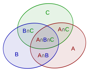
Example: The principle is more clearly seen in the case of three sets ( n = 3 ) 𝑛 3 (n=3) A , B 𝐴 𝐵
A,B C 𝐶 C
S = | A ∪ B ∪ C | = | A | + | B | + | C | − | A ∩ B | − | A ∩ C | − | B ∩ C | + | A ∩ B ∩ C | 𝑆 𝐴 𝐵 𝐶 𝐴 𝐵 𝐶 𝐴 𝐵 𝐴 𝐶 𝐵 𝐶 𝐴 𝐵 𝐶 S=|A\cup B\cup C|=|A|+|B|+|C|-|A\cap B|-|A\cap C|-|B\cap C|+|A\cap B\cap C|
Figure 1:
This formula can be verified by counting how many times each region in the Venn diagram (fig.1) figure is included in the right-hand side of the formula. In this case, when removing the contributions of overcounted elements, the number of elements in the mutual intersection of the three sets has been subtracted too often, so must be added back in to get the correct total.
This theory applies in our case both to the union of the principal fields of the basic functions and to
the subfields of the partial functions.
This method applies to polynomials with real or complex coefficients as well as transcedental polynomial formats. For such polynomials, we know that all complex roots appear as coupled pairs. The method attempts to locate the zeros of such polynomials by searching for zeros in a repetitive process after being split into two segments, and then in one section we calculate the inverse function that is the polynomial from mononym to until a trinomial. Therefore, we make the following reasoning, based on the theorem of continuity and if a function it has derivative and inverse.
From special to general method: Suppose we have the function f ( x ) = ∑ i = 0 n α i x i = 0 𝑓 𝑥 superscript subscript 𝑖 0 𝑛 subscript 𝛼 𝑖 superscript 𝑥 𝑖 0 f(x)=\displaystyle\sum_{i=0}^{n}\alpha_{i}x^{i}=0 f 1 ( x ) − f 2 ( x ) = 0 subscript 𝑓 1 𝑥 subscript 𝑓 2 𝑥 0 f_{1}(x)-f_{2}(x)=0 x x \mathrm{x} f 1 ( x ) = u subscript 𝑓 1 𝑥 𝑢 f_{1}(x)=u f 2 ( x ) = u subscript 𝑓 2 𝑥 𝑢 f_{2}(x)=u x k 1 = f 1 − 1 ( u ) = f 1 − 1 ( f 2 ( x m ) ) subscript 𝑥 subscript 𝑘 1 superscript subscript 𝑓 1 1 𝑢 superscript subscript 𝑓 1 1 subscript 𝑓 2 subscript 𝑥 𝑚 x_{k_{1}}=f_{1}^{-1}(u)=f_{1}^{-1}\left(f_{2}\left(x_{m}\right)\right) x k 2 = f 2 − 1 ( u ) = f 2 − 1 ( f 1 ( x m ) ) subscript 𝑥 subscript 𝑘 2 superscript subscript 𝑓 2 1 𝑢 superscript subscript 𝑓 2 1 subscript 𝑓 1 subscript 𝑥 𝑚 x_{k_{2}}=f_{2}^{-1}(u)=f_{2}^{-1}\left(f_{1}\left(x_{m}\right)\right) k 2 subscript 𝑘 2 k_{2} f 2 subscript 𝑓 2 f_{2} x k 2 r = f 2 − 1 ( f 1 ( x # ) ) , r = 0 , 1 , 2 , … N formulae-sequence superscript subscript 𝑥 subscript 𝑘 2 𝑟 superscript subscript 𝑓 2 1 subscript 𝑓 1 subscript 𝑥 # 𝑟 0 1 2 … 𝑁
x_{k_{2}}^{r}=f_{2}^{-1}\left(f_{1}\left(x_{\#}\right)\right),r=0,1,2,\ldots N r 𝑟 r N 𝑁 N f 1 ( x ) = ∑ i = 0 n − 1 a i x i , f 2 ( x ) = − a n x n formulae-sequence subscript 𝑓 1 𝑥 superscript subscript 𝑖 0 𝑛 1 subscript 𝑎 𝑖 superscript 𝑥 𝑖 subscript 𝑓 2 𝑥 subscript 𝑎 𝑛 superscript 𝑥 𝑛 f_{1}(x)=\displaystyle\sum_{i=0}^{n-1}a_{i}x^{i},f_{2}(x)=-a_{n}x^{n} G.R.L-N[1] the total of the roots will be the Union of the roots that will be found by the solution for the method (GRIM) for each monomial of polynomial ∑ i = 0 n a i x i = 0 superscript subscript 𝑖 0 𝑛 subscript 𝑎 𝑖 superscript 𝑥 𝑖 0 \displaystyle\sum_{i=0}^{n}a_{i}x^{i}=0 i 𝑖 i n 𝑛 n n 𝑛 n n 𝑛 n III.2.Theorem 2. Generalized Iterative Method approximation of Roots (GRIM)
We assume that we have general, elementary functions(in general transcendental) that are analytic except for some isolated singularities and branch cuts, in which case these and their local inversions will have convergent Taylor series expansions on suitable disks. Under these conditions for the determination of the roots any equation f ( x ) = ∑ i = 1 n a i σ i ( x ) − a 0 = 0 , { x , a i , a 0 ∈ ℂ , i ∈ ℕ + } ( 1 ) f(x)=\sum\limits_{i=1}^{n}a_{i}\sigma_{i}(x)-a_{0}=0,\ \{x,a_{i},a_{0}\in\mathbb{C},i\in\mathbb{N}^{+}\}\ (1) f : C → C : 𝑓 → 𝐶 𝐶 f:C\rightarrow C σ i ( x ) , 1 ≤ i ≤ n ∧ a i ∈ C subscript 𝜎 𝑖 𝑥 1
𝑖 𝑛 subscript 𝑎 𝑖 𝐶 \sigma_{i}(x),1\leq i\leq n\wedge a_{i}\in C σ 0 ( x ) = 1 subscript 𝜎 0 𝑥 1 \sigma_{0}(x)=1 G l , G 2 , … , G r , … G n subscript 𝐺 𝑙 subscript 𝐺 2 … subscript 𝐺 𝑟 … subscript 𝐺 𝑛
G_{l},G_{2},\ldots,G_{r},\ldots G_{n} k k \mathrm{k} G r , r ∈ { 1 , 2 , … , n } subscript 𝐺 𝑟 𝑟
1 2 … 𝑛 G_{r},r\in\{1,2,\ldots,n\} x 0 subscript 𝑥 0 x_{0} x 𝑥 x T T {}_{\text{T}} f ( x ) f x \mathrm{f}(\mathrm{x})
i ) σ r m r x k r μ \displaystyle i)\text{ }{}_{\sigma_{r}}^{m_{r}}x_{k_{r}}^{\mu} = σ r − 1 ( α 0 α r − 1 α r σ r c ( σ r − 1 ( α 0 α r − 1 α r σ r c ( σ r − 1 ( α 0 α r − … − \displaystyle=\sigma_{r}^{-1}\left(\frac{\alpha_{0}}{\alpha_{r}}-\frac{1}{\alpha_{r}}\sigma_{r}^{c}\left(\sigma_{r}^{-1}\left(\frac{\alpha_{0}}{\alpha_{r}}-\frac{1}{\alpha_{r}}\sigma_{r}^{c}\left(\sigma_{r}^{-1}\left(\frac{\alpha_{0}}{\alpha_{r}}-\ldots-\right.\right.\right.\right.\right.
− 1 α r σ r c ( σ r − 1 ( α 0 α r − 1 α r ⋅ ∑ i = 1 , i ≠ r n α i σ i ( x 0 ) ) ) ) ) ) ) ) , 1 < r ≤ n , 1 ≤ k ≤ ∞ \displaystyle\left.\left.\left.\left.\left.-\frac{1}{\alpha_{r}}\sigma_{r}^{c}\left(\sigma_{r}^{-1}\left(\frac{\alpha_{0}}{\alpha_{r}}-\frac{1}{\alpha_{r}}\cdot\sum_{\mathrm{i}=1,\mathrm{i}\neq\mathrm{r}}^{\mathrm{n}}\alpha_{i}\sigma_{\mathrm{i}}\left(\mathrm{x}_{0}\right)\right)\right)\right)\right)\right)\right)\right),1<\mathrm{r}\leq\mathrm{n},1\leq\mathrm{k}\leq\infty
i i ) σ r m r x k r μ \displaystyle ii)\text{ }{}_{\sigma_{r}}^{m_{r}}x_{k_{r}}^{\mu} = σ 1 − 1 ( α 0 α 1 − 1 α 1 σ 1 c ( σ 1 − 1 ( α 0 α 1 − 1 α 1 σ 1 c ( σ 1 − 1 ( α 0 α 1 − … − 1 α 1 σ 1 c ( σ 1 − 1 ( α 0 α 1 − \displaystyle=\sigma_{1}^{-1}\left(\frac{\alpha_{0}}{\alpha_{1}}-\frac{1}{\alpha_{1}}\sigma_{1}^{c}\left(\sigma_{1}^{-1}\left(\frac{\alpha_{0}}{\alpha_{1}}-\frac{1}{\alpha_{1}}\sigma_{1}^{c}\left(\sigma_{1}^{-1}\left(\frac{\alpha_{0}}{\alpha_{1}}-\ldots-\frac{1}{\alpha_{1}}\sigma_{1}^{c}\left(\sigma_{1}^{-1}\left(\frac{\alpha_{0}}{\alpha_{1}}-\right.\right.\right.\right.\right.\right.\right.
− 1 α 1 ⋅ ∑ i = 2 n α i σ i ( x 0 ) ) ) ) ) ) ) ) , r = 1 , 1 ≤ k ≤ ∞ \displaystyle\left.\left.\left.\left.\left.\left.\left.-\frac{1}{\alpha_{1}}\cdot\sum_{\mathrm{i}=2}^{\mathrm{n}}\alpha_{i}\sigma_{\mathrm{i}}\left(\mathrm{x}_{0}\right)\right)\right)\right)\right)\right)\right)\right),\mathrm{r}=1,1\leq\mathrm{k}\leq\infty
where σ r c superscript subscript 𝜎 𝑟 𝑐 \sigma_{r}^{c} σ r subscript 𝜎 𝑟 \sigma_{r} μ 𝜇 \mu T T {}_{\text{T}} Proof
For proof we go from the special to the general case. Suppose we have the function f [ x ] = ∑ i = 1 ∞ α i σ i ( x ) − α 0 = 0 𝑓 delimited-[] 𝑥 superscript subscript 𝑖 1 subscript 𝛼 𝑖 subscript 𝜎 𝑖 𝑥 subscript 𝛼 0 0 f[x]=\displaystyle\sum_{i=1}^{\infty}\alpha_{i}\sigma_{i}(x)-\alpha_{0}=0 f : C → C , α i ∈ C : 𝑓 formulae-sequence → 𝐶 𝐶 subscript 𝛼 𝑖 𝐶 f:C\rightarrow C,\alpha_{i}\in C α i subscript 𝛼 𝑖 \alpha_{i} f 1 ( x ) + f 2 ( x ) − α 0 = 0 subscript 𝑓 1 𝑥 subscript 𝑓 2 𝑥 subscript 𝛼 0 0 f_{1}(x)+f_{2}(x)-\alpha_{0}=0 f 1 ( x ) = a 1 σ 1 ( x ) ∧ f 2 ( x ) = ∑ i = 2 n a i σ i ( x ) ⇒ x j + 1 σ 1 = f 1 − 1 ( a 0 a 1 − 1 a 1 f 2 ( x j ) ) ( 3 ) subscript 𝑓 1 𝑥 subscript 𝑎 1 subscript 𝜎 1 𝑥 subscript 𝑓 2 𝑥 superscript subscript 𝑖 2 𝑛 subscript 𝑎 𝑖 subscript 𝜎 𝑖 𝑥 ⇒ subscript subscript 𝑥 𝑗 1 subscript 𝜎 1 superscript subscript 𝑓 1 1 subscript 𝑎 0 subscript 𝑎 1 1 subscript 𝑎 1 subscript 𝑓 2 subscript 𝑥 𝑗 3 f_{1}(x)=a_{1}\sigma_{1}(x)\wedge f_{2}(x)=\displaystyle\sum_{i=2}^{n}a_{i}\sigma_{i}(x)\Rightarrow{}_{\sigma_{1}}x_{j+1}=f_{1}^{-1}\left(\dfrac{a_{0}}{a_{1}}-\dfrac{1}{a_{1}}f_{2}\left(x_{j}\right)\right)\ (3) G 1 subscript 𝐺 1 G_{1}
x k 1 μ σ 1 m 1 subscript superscript superscript subscript 𝑥 subscript 𝑘 1 𝜇 subscript 𝑚 1 subscript 𝜎 1 \displaystyle{}_{\sigma_{1}}^{m_{1}}x_{k_{1}}^{\mu} = f 1 − 1 ( α 0 α 1 − 1 α 1 f 2 ( f 1 − 1 ( α 0 α 1 − 1 α 1 f 2 ( f 1 − 1 ( α 0 α 1 − … − 1 α 1 f 2 ( f 1 − 1 ( α 0 α 1 − 1 α 1 ∑ i = 2 n α i σ i ( x 0 ) ) ) ) ) ) ) ) absent superscript subscript f 1 1 subscript 𝛼 0 subscript 𝛼 1 1 subscript 𝛼 1 subscript f 2 superscript subscript f 1 1 subscript 𝛼 0 subscript 𝛼 1 1 subscript 𝛼 1 subscript f 2 superscript subscript f 1 1 subscript 𝛼 0 subscript 𝛼 1 … 1 subscript 𝛼 1 subscript f 2 superscript subscript f 1 1 subscript 𝛼 0 subscript 𝛼 1 1 subscript 𝛼 1 superscript subscript i 2 n subscript 𝛼 i subscript 𝜎 i subscript x 0 \displaystyle=\mathrm{f}_{1}^{-1}\left(\frac{\alpha_{0}}{\alpha_{1}}-\frac{1}{\alpha_{1}}\mathrm{f}_{2}\left(\mathrm{f}_{1}^{-1}\left(\frac{\alpha_{0}}{\alpha_{1}}-\frac{1}{\alpha_{1}}\mathrm{f}_{2}\left(\mathrm{f}_{1}^{-1}\left(\frac{\alpha_{0}}{\alpha_{1}}-\ldots-\frac{1}{\alpha_{1}}\mathrm{f}_{2}\left(\mathrm{f}_{1}^{-1}\left(\frac{\alpha_{0}}{\alpha_{1}}-\frac{1}{\alpha_{1}}\sum_{\mathrm{i}=2}^{\mathrm{n}}\alpha_{\mathrm{i}}\sigma_{\mathrm{i}}\left(\mathrm{x}_{0}\right)\right)\right)\right)\right)\right)\right)\right)
In general we have for m r subscript 𝑚 𝑟 m_{r} σ r subscript 𝜎 𝑟 \sigma_{r}
x k r μ σ r m r = f r − 1 ( α 0 α r − 1 α r f r c ( f r − 1 ( α 0 α r − 1 α r f r c ( f r − 1 ( α 0 α r − … − \displaystyle{}_{\sigma_{r}}^{m_{r}}x_{k_{r}}^{\mu}=\mathrm{f}_{\mathrm{r}}^{-1}\left(\frac{\alpha_{0}}{\alpha_{r}}-\frac{1}{\alpha_{r}}\mathrm{f}_{\mathrm{r}}^{\mathrm{c}}\left(\mathrm{f}_{\mathrm{r}}^{-1}\left(\frac{\alpha_{0}}{\alpha_{\mathrm{r}}}-\frac{1}{\alpha_{r}}\mathrm{f}_{\mathrm{r}}^{\mathrm{c}}\left(\mathrm{f}_{\mathrm{r}}^{-1}\left(\frac{\alpha_{0}}{\alpha_{r}}-\ldots-\right.\right.\right.\right.\right.
− 1 α r f r c ( f r − 1 ( α 0 α r − 1 α r ∑ i = 1 , i ≠ r n α i σ i ( x 0 ) ) ) ) ) ) ) ( 4 ) \displaystyle\left.\left.\left.\left.\left.-\frac{1}{\alpha_{r}}\mathrm{f}_{\mathrm{r}}^{\mathrm{c}}\left(\mathrm{f}_{\mathrm{r}}^{-1}\left(\frac{\alpha_{0}}{\alpha_{\mathrm{r}}}-\frac{1}{\alpha_{r}}\sum_{\mathrm{i}=1,\mathrm{i}\neq\mathrm{r}}^{\mathrm{n}}\alpha_{\mathrm{i}}\sigma_{\mathrm{i}}\left(\mathrm{x}_{0}\right)\right)\right)\right)\right)\right)\right)\right.(4)
where f r c superscript subscript 𝑓 𝑟 𝑐 f_{r}^{c} f r subscript 𝑓 𝑟 f_{r} x 0 subscript 𝑥 0 x_{0} x x \mathrm{x} μ 𝜇 \mu G 1 , G 2 , … , G r , … G n subscript 𝐺 1 subscript 𝐺 2 … subscript 𝐺 𝑟 … subscript 𝐺 𝑛
G_{1},G_{2},\ldots,G_{r},\ldots G_{n} σ r c ( x ) = ∑ i = 1 , i ≠ r n α i ⋅ σ i ( x ) superscript subscript 𝜎 r c x superscript subscript formulae-sequence i 1 i r n ⋅ subscript 𝛼 i subscript 𝜎 i x \sigma_{\mathrm{r}}^{\mathrm{c}}(\mathrm{x})=\sum\limits_{\mathrm{i}=1,\mathrm{i}\neq\mathrm{r}}^{\mathrm{n}}\alpha_{\mathrm{i}}\cdot\sigma_{\mathrm{i}}(\mathrm{x}) σ r ( x ) subscript 𝜎 r x \sigma_{\mathrm{r}}(\mathrm{x}) x 0 subscript 𝑥 0 x_{0} x 𝑥 x T T {}_{\text{T}} f ( x ) 𝑓 𝑥 f(x)
α 1 σ 1 ( x ) = − ( ∑ i = 2 n α i σ i ( x ) − α 0 ) ⇔ σ 1 ( x ) = − ( 1 α 1 ∑ i = 2 n α i σ i ( x ) − α 0 ) ⇔ subscript 𝛼 1 subscript 𝜎 1 𝑥 superscript subscript 𝑖 2 𝑛 subscript 𝛼 𝑖 subscript 𝜎 𝑖 𝑥 subscript 𝛼 0 subscript 𝜎 1 𝑥 1 subscript 𝛼 1 superscript subscript 𝑖 2 𝑛 subscript 𝛼 𝑖 subscript 𝜎 𝑖 𝑥 subscript 𝛼 0 \alpha_{1}\sigma_{1}(x)=-\left(\sum_{i=2}^{n}\alpha_{i}\sigma_{i}(x)-\alpha_{0}\right)\Leftrightarrow\sigma_{1}(x)=-\left(\frac{1}{\alpha_{1}}\sum_{i=2}^{n}\alpha_{i}\sigma_{i}(x)-\alpha_{0}\right)
⇔ x = σ 1 − 1 ( − ( 1 α 1 ∑ i = 2 n α i σ i ( x ) − α 0 ) ) ⇔ absent 𝑥 superscript subscript 𝜎 1 1 1 subscript 𝛼 1 superscript subscript 𝑖 2 𝑛 subscript 𝛼 𝑖 subscript 𝜎 𝑖 𝑥 subscript 𝛼 0 \Leftrightarrow x=\sigma_{1}^{-1}\left(-\left(\frac{1}{\alpha_{1}}\sum_{i=2}^{n}\alpha_{i}\sigma_{i}(x)-\alpha_{0}\right)\right)
and then apply for repeat with simple procedure x j + 1 σ r = σ r − 1 ( − 1 a r ( ∑ i ≠ r , i = 1 n α i ⋅ σ i ( x j ) − α 0 ) ) subscript subscript 𝑥 𝑗 1 subscript 𝜎 𝑟 superscript subscript 𝜎 𝑟 1 1 subscript 𝑎 𝑟 superscript subscript formulae-sequence 𝑖 𝑟 𝑖 1 𝑛 ⋅ subscript 𝛼 𝑖 subscript 𝜎 𝑖 subscript 𝑥 𝑗 subscript 𝛼 0 {}_{\sigma_{r}}x_{j+1}=\sigma_{r}^{-1}\left(-\dfrac{1}{a_{r}}\left(\displaystyle\sum_{i\neq r,i=1}^{n}\alpha_{i}\cdot\sigma_{i}\left(x_{j}\right)-\alpha_{0}\right)\right)
i ) σ k L k , q x s q μ \displaystyle i)\text{ }{}_{\sigma_{k}}^{L_{k,q}}x_{s_{q}}^{\mu} = σ k − 1 ( α 0 α k − 1 α k σ k c ( σ k − 1 ( α 0 α k − 1 α k σ k c ( σ k − 1 ( α 0 α k − … − \displaystyle=\sigma_{k}^{-1}\left(\frac{\alpha_{0}}{\alpha_{k}}-\frac{1}{\alpha_{k}}\sigma_{k}^{c}\left(\sigma_{k}^{-1}\left(\frac{\alpha_{0}}{\alpha_{k}}-\frac{1}{\alpha_{k}}\sigma_{k}^{c}\left(\sigma_{k}^{-1}\left(\frac{\alpha_{0}}{\alpha_{k}}-\ldots-\right.\right.\right.\right.\right.
− 1 α k σ k c ( σ k − 1 ( α 0 α k − 1 α k ⋅ ∑ i = 1 , i ≠ k n α i σ i ( x 0 ) ) ) ) ) ) ) ) \displaystyle-\left.\left.\left.\left.\left.\frac{1}{\alpha_{k}}\sigma_{k}^{c}\left(\sigma_{k}^{-1}\left(\frac{\alpha_{0}}{\alpha_{k}}-\frac{1}{\alpha_{k}}\cdot\sum_{i=1,i\neq k}^{n}\alpha_{i}\sigma_{i}\left(x_{0}\right)\right)\right)\right)\right)\right)\right)\right)
if 1 < k ≤ n , 0 ≤ s ≤ ∞ , q ∈ N + , formulae-sequence if 1 k n 0 s q superscript N , \displaystyle\text{ if }1<\mathrm{k}\leq\mathrm{n},0\leq\mathrm{s}\leq\infty,\mathrm{q}\in\mathrm{N}^{+}\text{, }
i i ) σ k L k , q x s q μ \displaystyle ii)\text{ }{}_{\sigma_{k}}^{L_{k,q}}x_{s_{q}}^{\mu} = σ 1 − 1 ( α 0 α 1 − 1 α 1 σ 1 c ( σ 1 − 1 ( α 0 α 1 − 1 α 1 σ 1 c ( σ 1 − 1 ( α 0 α 1 − … − \displaystyle=\sigma_{1}^{-1}\left(\frac{\alpha_{0}}{\alpha_{1}}-\frac{1}{\alpha_{1}}\sigma_{1}^{c}\left(\sigma_{1}^{-1}\left(\frac{\alpha_{0}}{\alpha_{1}}-\frac{1}{\alpha_{1}}\sigma_{1}^{c}\left(\sigma_{1}^{-1}\left(\frac{\alpha_{0}}{\alpha_{1}}-\ldots-\right.\right.\right.\right.\right.
− \displaystyle- 1 α 1 σ 1 c ( σ 1 − 1 ( α 0 α 1 − 1 α 1 ⋅ ∑ i = 2 n α i σ i ( x 0 ) ) ) ) ) ) ) ) \displaystyle\left.\left.\left.\left.\left.\frac{1}{\alpha_{1}}\sigma_{1}^{c}\left(\sigma_{1}^{-1}\left(\frac{\alpha_{0}}{\alpha_{1}}-\frac{1}{\alpha_{1}}\cdot\sum_{i=2}^{n}\alpha_{i}\sigma_{i}\left(x_{0}\right)\right)\right)\right)\right)\right)\right)\right)
if k = 1 , 0 ≤ s ≤ ∞ , q ∈ N + formulae-sequence formulae-sequence if k 1 0 s q superscript N \displaystyle\text{ if }\mathrm{k}=1,0\leq\mathrm{s}\leq\infty,\mathrm{q}\in\mathrm{N}^{+}
Apply : α k σ k ( x ) + σ k c ( x ) − α 0 = 0 ∧ σ k c ( x ) = ∑ i = 1 , i ≠ k n α i σ i ( x ) where σ k c the complement of σ k . : Apply subscript 𝛼 𝑘 subscript 𝜎 𝑘 𝑥 superscript subscript 𝜎 𝑘 𝑐 𝑥 subscript 𝛼 0 0 superscript subscript 𝜎 𝑘 𝑐 𝑥 superscript subscript formulae-sequence 𝑖 1 𝑖 𝑘 𝑛 subscript 𝛼 𝑖 subscript 𝜎 𝑖 𝑥 where superscript subscript 𝜎 k c the complement of subscript 𝜎 𝑘 \text{Apply}:\alpha_{k}\sigma_{k}(x)+\sigma_{k}^{c}(x)-\alpha_{0}=0\wedge\sigma_{k}^{c}(x)=\sum_{i=1,i\neq k}^{n}\alpha_{i}\sigma_{i}(x)\text{ where }\sigma_{\mathrm{k}}^{\mathrm{c}}\text{ the complement of }\sigma_{k}.
where σ r c superscript subscript 𝜎 𝑟 𝑐 \sigma_{r}^{c} σ r subscript 𝜎 𝑟 \sigma_{r} μ 𝜇 \mu m r subscript 𝑚 𝑟 m_{r} G r , r ∈ { 1 , 2 , … , n } subscript 𝐺 𝑟 𝑟
1 2 … 𝑛 G_{r},r\in\{1,2,\ldots,n\} x 0 subscript x 0 \mathrm{x}_{0} x x \mathrm{x} T T {}_{\text{T}} Part IV. Solved examples with the method (GRIM) [2,3,4,5]
α 1 z r 1 ⋅ a z q 1 + α 2 ⋅ z r 2 ⋅ b z q 2 − α 0 = 0 ( α i , r i , q i , a , b ∈ C , i = 1 , 2 ∧ α 0 ∈ C ) \alpha_{1}z^{r_{1}}\cdot a^{z^{q_{1}}}+\alpha_{2}\cdot z^{r_{2}}\cdot b^{z^{q_{2}}}-\alpha_{0}=0\ \left(\alpha_{i},r_{i},q_{i},a,b\in C,i=1,2\wedge\alpha_{0}\in C\right)
IV.1.2. We have the general equation with relation f ( z ) = ∑ i = 1 2 α i ⋅ σ i ( z ) − α 0 = 0 , { r i , q i , α i , α 0 ∈ C , i = 1 , 2 } f(z)=\sum\limits_{i=1}^{2}\alpha_{i}\cdot\sigma_{i}(z)-\alpha_{0}=0,\left\{r_{i},q_{i},\alpha_{i},\alpha_{0}\in C,i=1,2\right\} σ 1 ( z ) = z r 1 ⋅ a z q 1 ∧ σ 2 ( z ) = z r 2 ⋅ b z q 2 subscript 𝜎 1 𝑧 ⋅ superscript 𝑧 subscript 𝑟 1 superscript 𝑎 superscript 𝑧 subscript 𝑞 1 subscript 𝜎 2 𝑧 ⋅ superscript 𝑧 subscript 𝑟 2 superscript 𝑏 superscript 𝑧 subscript 𝑞 2 \sigma_{1}(z)=z^{r_{1}}\cdot a^{z^{q_{1}}}\wedge\sigma_{2}(z)=z^{r_{2}}\cdot b^{z^{q_{2}}} σ 1 ( z ) = z r 1 ⋅ a z q i , r 1 , q 1 ∈ C formulae-sequence subscript 𝜎 1 𝑧 ⋅ superscript 𝑧 subscript 𝑟 1 superscript 𝑎 superscript 𝑧 subscript 𝑞 𝑖 subscript 𝑟 1
subscript 𝑞 1 𝐶 \sigma_{1}(z)=z^{r_{1}}\cdot a^{z^{q_{i}}},r_{1},q_{1}\in C first term function to a variable, suppose u 𝑢 u
σ 1 ( z ) = z r 1 ⋅ a z q 1 = u ⇔ r 1 log z + z q 1 log a = log u + 2 k π I , q 1 ≠ 0 , k ∈ Z ⇔ subscript 𝜎 1 𝑧 ⋅ superscript 𝑧 subscript 𝑟 1 superscript 𝑎 superscript 𝑧 subscript 𝑞 1 𝑢 formulae-sequence subscript 𝑟 1 𝑧 superscript 𝑧 subscript 𝑞 1 𝑎 𝑢 2 𝑘 𝜋 𝐼 formulae-sequence subscript 𝑞 1 0 𝑘 𝑍 \sigma_{1}(z)=z^{r_{1}}\cdot a^{z^{q_{1}}}=u\Leftrightarrow r_{1}\log z+z^{q_{1}}\log a=\log u+2k\pi I,q_{1}\neq 0,k\in Z
From ( 1 ) ⇔ ( r 1 q 1 ) ⋅ log z q 1 + z q 1 log a = log u + 2 k π I ( 2 ) , I : ⇔ 1 ⋅ subscript 𝑟 1 subscript 𝑞 1 superscript 𝑧 subscript 𝑞 1 superscript 𝑧 subscript 𝑞 1 𝑎 𝑢 2 𝑘 𝜋 𝐼 2 𝐼
: absent (1)\Leftrightarrow\left(\frac{r_{1}}{q_{1}}\right)\cdot\log z^{q_{1}}+z^{q_{1}}\log a=\log u+2k\pi I(2),\ I: z q 1 = y superscript 𝑧 subscript 𝑞 1 𝑦 z^{q_{1}}=y
( r 1 q 1 ) ⋅ log y + y log a = log u + 2 k π I . ⋅ subscript 𝑟 1 subscript 𝑞 1 𝑦 𝑦 𝑎 𝑢 2 𝑘 𝜋 𝐼 \left(\frac{r_{1}}{q_{1}}\right)\cdot\log y+y\log a=\log u+2k\pi I.
The point here is to relate variable y 𝑦 y
t y ⋅ e t y = s ( 5 ) ⇔ t y = W ( k 1 , s ) ⇔ y = W ( k 1 , s ) t ( 6 ) , { s , t ∈ C , t ≠ 0 , k 1 ∈ Z } ty\cdot e^{ty}=s\ (5)\Leftrightarrow ty=W\left(k_{1},s\right)\Leftrightarrow y=\frac{W\left(k_{1},s\right)}{t}\ (6),\ \left\{s,t\in C,t\neq 0,k_{1}\in Z\right\}
If I now logarithmize relationship (5), I obtain the relationship
t y ⋅ e t y = s ⇔ log y + t y = log s t + 2 k π I ⇔ ⋅ 𝑡 𝑦 superscript 𝑒 𝑡 𝑦 𝑠 𝑦 𝑡 𝑦 𝑠 𝑡 2 𝑘 𝜋 𝐼 ty\cdot e^{ty}=s\Leftrightarrow\log y+ty=\log\frac{s}{t}+2k\pi I
Combining ( 4 , 7 ) 4 7 (4,7)
t = log a r 1 q 1 ( 8 ) ∧ u q 1 r 1 = s t ( 9 ) 𝑡 𝑎 subscript 𝑟 1 subscript 𝑞 1 8 superscript 𝑢 subscript 𝑞 1 subscript 𝑟 1 𝑠 𝑡 9 t=\frac{\log a}{\frac{r_{1}}{q_{1}}}\ (8)\wedge u^{\frac{q_{1}}{r_{1}}}=\frac{s}{t}\ (9)
By combining relations ( 3 , 6 , 8 , 9 ) 3 6 8 9 (3,6,8,9)
z 1 = { ( r 1 q 1 ⋅ log a ) ⋅ W ( k 1 , log a r 1 q 11 ⋅ u q 1 r 1 ) } 1 q 1 ⋅ e 2 k 2 π ⋅ I q 1 ( 10 ) , { k 2 , k 1 ∈ Z } , k 2 = 1 ÷ q 1 − 1 formulae-sequence subscript 𝑧 1 ⋅ superscript ⋅ subscript 𝑟 1 ⋅ subscript 𝑞 1 𝑎 𝑊 subscript 𝑘 1 ⋅ 𝑎 subscript 𝑟 1 subscript 𝑞 11 superscript 𝑢 subscript 𝑞 1 subscript 𝑟 1 1 subscript 𝑞 1 superscript 𝑒 ⋅ 2 subscript 𝑘 2 𝜋 I subscript 𝑞 1 10 subscript 𝑘 2 subscript 𝑘 1
𝑍
subscript 𝑘 2 1 subscript 𝑞 1 1 z_{1}=\left\{\left(\frac{r_{1}}{q_{1}\cdot\log a}\right)\cdot W\left(k_{1},\frac{\log a}{\frac{r_{1}}{q_{11}}}\cdot u^{\frac{q_{1}}{r_{1}}}\right)\right\}^{\frac{1}{q_{1}}}\cdot e^{\frac{2k_{2}\pi\cdot\mathrm{I}}{q_{1}}}(10),\left\{k_{2},k_{1}\in Z\right\},k_{2}=1\div q_{1}-1
In the same way we calculate for the second kernel the relation
z 2 = { ( r 2 q 2 ⋅ log b ) ⋅ W ( k 1 ′ , log b r 2 q 2 ⋅ u q 2 r 2 ) } 1 q 2 ⋅ e 2 k 2 ′ π ⋅ I q 2 ( 10 ) , { k 1 ′ , k 2 ′ ∈ Z } , k 2 ′ = 1 ÷ q 2 − 1 formulae-sequence subscript 𝑧 2 ⋅ superscript ⋅ subscript 𝑟 2 ⋅ subscript 𝑞 2 𝑏 𝑊 superscript subscript 𝑘 1 ′ ⋅ 𝑏 subscript 𝑟 2 subscript 𝑞 2 superscript 𝑢 subscript 𝑞 2 𝑟 2 1 subscript 𝑞 2 superscript 𝑒 ⋅ 2 superscript subscript 𝑘 2 ′ 𝜋 I subscript 𝑞 2 10 superscript subscript 𝑘 1 ′ superscript subscript 𝑘 2 ′
𝑍
superscript subscript 𝑘 2 ′ 1 subscript 𝑞 2 1 z_{2}=\left\{\left(\frac{r_{2}}{q_{2}\cdot\log b}\right)\cdot W\left(k_{1}^{\prime},\frac{\log b}{\frac{r_{2}}{q_{2}}}\cdot u^{\frac{q_{2}}{r2}}\right)\right\}^{\frac{1}{q_{2}}}\cdot e^{\frac{2k_{2}^{\prime}\pi\cdot\mathrm{I}}{q_{2}}}\ \ (10),\left\{k_{1}^{\prime},k_{2}^{\prime}\in Z\right\},k_{2}^{\prime}=1\div q_{2}-1
Up to this point we have developed the concept of the iteration process. But the basic GRT T {}_{\text{T}} σ 1 ( z ) = z r 1 ⋅ a z q 1 ∧ σ 2 ( z ) = z r 2 ⋅ b z q 2 subscript 𝜎 1 𝑧 ⋅ superscript 𝑧 subscript 𝑟 1 superscript 𝑎 superscript 𝑧 subscript 𝑞 1 subscript 𝜎 2 𝑧 ⋅ superscript 𝑧 subscript 𝑟 2 superscript 𝑏 superscript 𝑧 subscript 𝑞 2 \sigma_{1}(z)=z^{r_{1}}\cdot a^{z^{q_{1}}}\wedge\sigma_{2}(z)=z^{r_{2}}\cdot b^{z^{q_{2}}} T T {}_{\text{T}} σ 1 ( z ) , σ 2 ( z ) subscript 𝜎 1 𝑧 subscript 𝜎 2 𝑧
\sigma_{1}(z),\sigma_{2}(z) σ 1 ( z ) = z r 1 ⋅ a z q 1 ∧ σ 2 ( z ) = z r 2 ⋅ b z q 2 subscript 𝜎 1 𝑧 ⋅ superscript 𝑧 subscript 𝑟 1 superscript 𝑎 superscript 𝑧 subscript 𝑞 1 subscript 𝜎 2 𝑧 ⋅ superscript 𝑧 subscript 𝑟 2 superscript 𝑏 superscript 𝑧 subscript 𝑞 2 \sigma_{1}(z)=z^{r_{1}}\cdot a^{z^{q_{1}}}\wedge\sigma_{2}(z)=z^{r_{2}}\cdot b^{z^{q_{2}}} L 1 , L 2 subscript 𝐿 1 subscript 𝐿 2
L_{1},L_{2} L = L 1 ∪ L 2 𝐿 subscript 𝐿 1 subscript 𝐿 2 L=L_{1}\cup L_{2} IV.1.3. Finding the L 𝟏 subscript 𝐿 1 \boldsymbol{L_{1}} The first roots of sub-field L 1 subscript 𝐿 1 L_{1}
σ 1 ( z ) = u ⇒ z { s 1 , s 2 } L 1 = { ( r 1 q 1 ⋅ log a ) ⋅ W ( s 1 , log a r 1 q 1 ⋅ u q 1 r 1 ) } 1 q 1 ⋅ e 2 s 2 π ⋅ I q 1 , { s 2 , s 1 ∈ Z } , s 2 = 0 ÷ q 1 − 1 formulae-sequence subscript 𝜎 1 𝑧 𝑢 ⇒ superscript subscript 𝑧 subscript 𝑠 1 subscript 𝑠 2 subscript 𝐿 1 ⋅ superscript ⋅ subscript 𝑟 1 ⋅ subscript 𝑞 1 𝑎 𝑊 subscript 𝑠 1 ⋅ 𝑎 subscript 𝑟 1 subscript 𝑞 1 superscript 𝑢 subscript 𝑞 1 subscript 𝑟 1 1 subscript 𝑞 1 superscript 𝑒 ⋅ 2 subscript 𝑠 2 𝜋 I subscript 𝑞 1 subscript 𝑠 2 subscript 𝑠 1
𝑍 subscript 𝑠 2
0 subscript 𝑞 1 1 \sigma_{1}(z)=u\Rightarrow z_{\left\{s_{1},s_{2}\right\}}^{L_{1}}=\left\{\left(\frac{r_{1}}{q_{1}\cdot\log a}\right)\cdot W\left(s_{1},\frac{\log a}{\frac{r_{1}}{q_{1}}}\cdot u^{\frac{q_{1}}{r_{1}}}\right)\right\}^{\frac{1}{q_{1}}}\cdot e^{\frac{2s_{2}\pi\cdot\mathrm{I}}{q_{1}}},\left\{s_{2},s_{1}\in Z\right\},s_{2}=0\div q_{1}-1
So, using this method (GRIP) we will have 1 relation to find the set of solutions of the first subfield. We talk about 𝒒 𝟏 subscript 𝒒 1 \boldsymbol{q_{1}} Categories of infinite (by parameter s 𝟏 subscript 𝑠 1 \boldsymbol{s_{1}} complex roots.
IV.1.4. Finding the L 𝟐 subscript 𝐿 2 \boldsymbol{L_{2}} The second roots of sub-field L 2 subscript 𝐿 2 L_{2}
σ 2 ( z ) = u ⇒ z { s 1 ′ , s 2 ′ } L 2 = { ( r 2 q 2 ⋅ log b ) ⋅ W ( s 1 ′ , log b r 2 q 2 ⋅ u q 2 r 2 ) } 1 q 2 ⋅ e 2 s 2 ′ π ⋅ I q 2 , { s 2 ′ , s 1 ′ ∈ Z } , s 2 ′ = 0 ÷ q 2 − 1 formulae-sequence subscript 𝜎 2 𝑧 𝑢 ⇒ superscript subscript 𝑧 superscript subscript 𝑠 1 ′ superscript subscript 𝑠 2 ′ subscript 𝐿 2 ⋅ superscript ⋅ subscript 𝑟 2 ⋅ subscript 𝑞 2 𝑏 𝑊 superscript subscript 𝑠 1 ′ ⋅ 𝑏 subscript 𝑟 2 subscript 𝑞 2 superscript 𝑢 subscript 𝑞 2 subscript 𝑟 2 1 subscript 𝑞 2 superscript 𝑒 ⋅ 2 superscript subscript 𝑠 2 ′ 𝜋 I subscript 𝑞 2 superscript subscript 𝑠 2 ′ superscript subscript 𝑠 1 ′
𝑍 superscript subscript 𝑠 2 ′
0 subscript 𝑞 2 1 \sigma_{2}(z)=u\Rightarrow z_{\left\{s_{1}^{\prime},s_{2}^{\prime}\right\}}^{L_{2}}=\left\{\left(\frac{r_{2}}{q_{2}\cdot\log b}\right)\cdot W\left(s_{1}^{\prime},\frac{\log b}{\frac{r_{2}}{q_{2}}}\cdot u^{\frac{q_{2}}{r_{2}}}\right)\right\}^{\frac{1}{q_{2}}}\cdot e^{\frac{2s_{2}^{\prime}\pi\cdot\mathrm{I}}{q_{2}}},\left\{s_{2}^{\prime},s_{1}^{\prime}\in Z\right\},s_{2}^{\prime}=0\div q_{2}-1
So, using this method (GRIP) we will have 1 relation to find the set of solutions of the second subfield. We talk about 𝒒 𝟐 subscript 𝒒 2 \boldsymbol{q_{2}} Categories of infinite (by parameter s 𝟏 ′ superscript subscript 𝑠 1 bold-′ \boldsymbol{s_{1}^{\prime}} complex roots.
IV.1.5. Iterative Method approximation of Roots.
In our case we have 2 functions, with one Sub-fields per function, which means that for the set of solutions of the field L 𝐿 L L = L 1 ∪ L 2 𝐿 subscript 𝐿 1 subscript 𝐿 2 L=L_{1}\cup L_{2} L 1 subscript 𝐿 1 L_{1} σ 1 ( z ) subscript 𝜎 1 𝑧 \sigma_{1}(z)
z s q μ σ 1 L 1 , q = σ 1 − 1 ( α 0 α 1 − 1 α 1 σ 1 c ( σ 1 − 1 ( α 0 α 1 − 1 α 1 σ 1 c ( σ 1 − 1 ( α 0 α 1 − … − {}_{\sigma_{1}}^{L_{1,q}}z_{s_{q}}^{\mu}=\sigma_{1}^{-1}\left(\frac{\alpha_{0}}{\alpha_{1}}-\frac{1}{\alpha_{1}}\sigma_{1}^{c}\left(\sigma_{1}^{-1}\left(\frac{\alpha_{0}}{\alpha_{1}}-\frac{1}{\alpha_{1}}\sigma_{1}^{c}\left(\sigma_{1}^{-1}\left(\frac{\alpha_{0}}{\alpha_{1}}-\ldots-\right.\right.\right.\right.\right.
− 1 α 1 σ 1 c ( σ 1 − 1 ( α 0 α 1 − 1 α 1 ⋅ ∑ i = 2 2 α i σ i ( z 0 ) ) ) ) ) ) ) ) , 1 ≤ k ≤ 2 , 0 ≤ s ≤ ∞ , q ∈ ℕ + , \left.\left.\left.\left.\left.-\frac{1}{\alpha_{1}}\sigma_{1}^{c}\left(\sigma_{1}^{-1}\left(\frac{\alpha_{0}}{\alpha_{1}}-\frac{1}{\alpha_{1}}\cdot\sum\limits_{\mathrm{i}=2}^{2}\alpha_{\mathrm{i}}\sigma_{\mathrm{i}}\left(\mathrm{z}_{0}\right)\right)\right)\right)\right)\right)\right)\right),1\leq k\leq 2,\ 0\leq s\leq\infty,q\in\mathbb{N}^{+},
Apply: α 1 σ 1 ( z ) + σ 1 c ( z ) − α 0 = 0 ∧ σ 1 c ( z ) = ∑ i = 2 2 α 2 σ i ( z ) = α 2 ⋅ z r 2 ⋅ b z q 2 subscript 𝛼 1 subscript 𝜎 1 𝑧 superscript subscript 𝜎 1 𝑐 𝑧 subscript 𝛼 0 0 superscript subscript 𝜎 1 𝑐 𝑧 superscript subscript 𝑖 2 2 subscript 𝛼 2 subscript 𝜎 𝑖 𝑧 ⋅ subscript 𝛼 2 superscript 𝑧 subscript 𝑟 2 superscript 𝑏 superscript 𝑧 subscript 𝑞 2 \alpha_{1}\sigma_{1}(z)+\sigma_{1}^{c}(z)-\alpha_{0}=0\wedge\sigma_{1}^{c}(z)=\sum\limits_{i=2}^{2}\alpha_{2}\sigma_{i}(z)=\alpha_{2}\cdot z^{r_{2}}\cdot b^{z^{q_{2}}}
σ 1 − 1 ( z ) = { ( r 1 q 1 ⋅ log a ) ⋅ W ( s 1 , log a r 1 q 1 ⋅ u q 1 r 1 ) } 1 q 1 ⋅ e 2 s 2 π ⋅ I q 1 , { s 2 , s 1 ∈ Z } , s 2 = 0 ÷ q 1 − 1 formulae-sequence superscript subscript 𝜎 1 1 𝑧 ⋅ superscript ⋅ subscript 𝑟 1 ⋅ subscript 𝑞 1 𝑎 𝑊 subscript 𝑠 1 ⋅ 𝑎 subscript 𝑟 1 subscript 𝑞 1 superscript 𝑢 subscript 𝑞 1 subscript 𝑟 1 1 subscript 𝑞 1 superscript 𝑒 ⋅ 2 subscript 𝑠 2 𝜋 𝐼 subscript 𝑞 1 subscript 𝑠 2 subscript 𝑠 1
𝑍
subscript 𝑠 2 0 subscript 𝑞 1 1 \sigma_{1}^{-1}(z)=\left\{\left(\frac{r_{1}}{q_{1}\cdot\log a}\right)\cdot W\left(s_{1},\frac{\log a}{\frac{r_{1}}{q_{1}}}\cdot u^{\frac{q_{1}}{r_{1}}}\right)\right\}^{\frac{1}{q_{1}}}\cdot e^{\frac{2s_{2}\pi\cdot I}{q_{1}}},\left\{s_{2},s_{1}\in Z\right\},s_{2}=0\div q_{1}-1
where σ 1 c superscript subscript 𝜎 1 c \sigma_{1}^{\mathrm{c}} σ 1 subscript 𝜎 1 \sigma_{1} α 2 subscript 𝛼 2 \alpha_{2} L 2 subscript 𝐿 2 L_{2} σ 2 ( z ) subscript 𝜎 2 𝑧 \sigma_{2}(z)
z s q ′ μ σ 2 L 2 , q ′ = σ 2 − 1 ( α 0 α 2 − 1 α 2 σ 2 c ( σ 2 − 1 ( α 0 α 2 − 1 α 2 σ 2 c ( σ 2 − 1 ( α 0 α 2 − … − {}_{\sigma_{2}}^{L_{2,q^{\prime}}}z_{s_{q^{\prime}}}^{\mu}=\sigma_{2}^{-1}\left(\frac{\alpha_{0}}{\alpha_{2}}-\frac{1}{\alpha_{2}}\sigma_{2}^{c}\left(\sigma_{2}^{-1}\left(\frac{\alpha_{0}}{\alpha_{2}}-\frac{1}{\alpha_{2}}\sigma_{2}^{c}\left(\sigma_{2}^{-1}\left(\frac{\alpha_{0}}{\alpha_{2}}-\ldots-\right.\right.\right.\right.\right.
− 1 α 2 σ 2 c ( σ 2 − 1 ( α 0 α 2 − 1 α 2 ⋅ ∑ i = 1 1 α i σ i ( z 0 ) ) ) ) ) ) ) ) , k = 2 , 0 ≤ s ≤ ∞ , q ∈ ℕ + , \left.\left.\left.\left.\left.-\frac{1}{\alpha_{2}}\sigma_{2}^{c}\left(\sigma_{2}^{-1}\left(\frac{\alpha_{0}}{\alpha_{2}}-\frac{1}{\alpha_{2}}\cdot\sum\limits_{\mathrm{i}=1}^{1}\alpha_{\mathrm{i}}\sigma_{\mathrm{i}}\left(\mathrm{z}_{0}\right)\right)\right)\right)\right)\right)\right)\right),k=2,\ 0\leq s\leq\infty,q\in\mathbb{N}^{+},
Apply: α 2 σ 2 ( z ) + σ 2 c ( z ) − α 0 = 0 ∧ σ 2 c ( z ) = ∑ i = 1 1 α 1 σ i ( z ) = α 1 ⋅ z r 1 ⋅ b z q 1 subscript 𝛼 2 subscript 𝜎 2 𝑧 superscript subscript 𝜎 2 𝑐 𝑧 subscript 𝛼 0 0 superscript subscript 𝜎 2 𝑐 𝑧 superscript subscript 𝑖 1 1 subscript 𝛼 1 subscript 𝜎 𝑖 𝑧 ⋅ subscript 𝛼 1 superscript 𝑧 subscript 𝑟 1 superscript 𝑏 superscript 𝑧 subscript 𝑞 1 \alpha_{2}\sigma_{2}(z)+\sigma_{2}^{c}(z)-\alpha_{0}=0\wedge\sigma_{2}^{c}(z)=\sum\limits_{i=1}^{1}\alpha_{1}\sigma_{i}(z)=\alpha_{1}\cdot z^{r_{1}}\cdot b^{z^{q_{1}}}
σ 2 − 1 ( z ) = { ( r 2 q 2 ⋅ log b ) ⋅ W ( s 1 ′ , log b r 2 q 2 ⋅ u q 2 r 2 ) } 1 q 2 ⋅ e 2 s 2 ′ π ⋅ I q 2 , { s 2 , s 1 ∈ Z } , s 2 = 0 ÷ q 2 − 1 formulae-sequence superscript subscript 𝜎 2 1 𝑧 ⋅ superscript ⋅ subscript 𝑟 2 ⋅ subscript 𝑞 2 𝑏 𝑊 subscript superscript 𝑠 ′ 1 ⋅ 𝑏 subscript 𝑟 2 subscript 𝑞 2 superscript 𝑢 subscript 𝑞 2 subscript 𝑟 2 1 subscript 𝑞 2 superscript 𝑒 ⋅ 2 subscript superscript 𝑠 ′ 2 𝜋 𝐼 subscript 𝑞 2 subscript 𝑠 2 subscript 𝑠 1
𝑍
subscript 𝑠 2 0 subscript 𝑞 2 1 \sigma_{2}^{-1}(z)=\left\{\left(\frac{r_{2}}{q_{2}\cdot\log b}\right)\cdot W\left(s^{\prime}_{1},\frac{\log b}{\frac{r_{2}}{q_{2}}}\cdot u^{\frac{q_{2}}{r_{2}}}\right)\right\}^{\frac{1}{q_{2}}}\cdot e^{\frac{2s^{\prime}_{2}\pi\cdot I}{q_{2}}},\left\{s_{2},s_{1}\in Z\right\},s_{2}=0\div q_{2}-1
where σ 2 c superscript subscript 𝜎 2 c \sigma_{2}^{\mathrm{c}} σ 2 subscript 𝜎 2 \sigma_{2} α 1 subscript 𝛼 1 \alpha_{1} IV.1.6. We will look at a real example. We will look at a real example. Solve equation x ⋅ α 1 x + 1 x α x = 2 a ⋅ 𝑥 superscript 𝛼 1 𝑥 1 𝑥 superscript 𝛼 𝑥 2 𝑎 x\cdot\alpha^{\frac{1}{x}}+\frac{1}{x}\alpha^{x}=2a L 1 subscript 𝐿 1 L_{1} σ 1 ( z ) subscript 𝜎 1 𝑧 \sigma_{1}(z)
α 1 = 1 , α 2 = 1 , r 1 = 1 , q 1 = − 1 , a = α , b = α , α 0 = 2 α , r 2 = − 1 , q 2 = 1 formulae-sequence subscript 𝛼 1 1 formulae-sequence subscript 𝛼 2 1 formulae-sequence subscript 𝑟 1 1 formulae-sequence subscript 𝑞 1 1 formulae-sequence 𝑎 𝛼 formulae-sequence 𝑏 𝛼 formulae-sequence subscript 𝛼 0 2 𝛼 formulae-sequence subscript 𝑟 2 1 subscript 𝑞 2 1 \alpha_{1}=1,\alpha_{2}=1,r_{1}=1,q_{1}=-1,a=\alpha,b=\alpha,\alpha_{0}=2\alpha,r_{2}=-1,q_{2}=1
z s q μ σ 1 L 1 , q = σ 1 − 1 ( α 0 α 1 − 1 α 1 σ 1 c ( σ 1 − 1 ( α 0 α 1 − 1 α 1 σ 1 c ( σ 1 − 1 ( α 0 α 1 − … − {}_{\sigma_{1}}^{L_{1,q}}z_{s_{q}}^{\mu}=\sigma_{1}^{-1}\left(\frac{\alpha_{0}}{\alpha_{1}}-\frac{1}{\alpha_{1}}\sigma_{1}^{c}\left(\sigma_{1}^{-1}\left(\frac{\alpha_{0}}{\alpha_{1}}-\frac{1}{\alpha_{1}}\sigma_{1}^{c}\left(\sigma_{1}^{-1}\left(\frac{\alpha_{0}}{\alpha_{1}}-\ldots-\right.\right.\right.\right.\right.
− 1 α 1 σ 1 c ( σ 1 − 1 ( α 0 α 1 − 1 α 1 ⋅ ∑ i = 2 2 α i σ i ( z 0 ) ) ) ) ) ) ) ) , 1 ≤ k ≤ 2 , 0 ≤ s ≤ ∞ , q ∈ ℕ + , \left.\left.\left.\left.\left.-\frac{1}{\alpha_{1}}\sigma_{1}^{c}\left(\sigma_{1}^{-1}\left(\frac{\alpha_{0}}{\alpha_{1}}-\frac{1}{\alpha_{1}}\cdot\sum\limits_{\mathrm{i}=2}^{2}\alpha_{\mathrm{i}}\sigma_{\mathrm{i}}\left(\mathrm{z}_{0}\right)\right)\right)\right)\right)\right)\right)\right),1\leq k\leq 2,\ 0\leq s\leq\infty,q\in\mathbb{N}^{+},
Apply: α 1 σ 1 ( z ) + σ 1 c ( z ) − α 0 = 0 ∧ σ 1 c ( z ) = ∑ i = 2 2 α 2 σ i ( z ) = α 2 ⋅ z r 2 ⋅ b z q 2 subscript 𝛼 1 subscript 𝜎 1 𝑧 superscript subscript 𝜎 1 𝑐 𝑧 subscript 𝛼 0 0 superscript subscript 𝜎 1 𝑐 𝑧 superscript subscript 𝑖 2 2 subscript 𝛼 2 subscript 𝜎 𝑖 𝑧 ⋅ subscript 𝛼 2 superscript 𝑧 subscript 𝑟 2 superscript 𝑏 superscript 𝑧 subscript 𝑞 2 \alpha_{1}\sigma_{1}(z)+\sigma_{1}^{c}(z)-\alpha_{0}=0\wedge\sigma_{1}^{c}(z)=\sum\limits_{i=2}^{2}\alpha_{2}\sigma_{i}(z)=\alpha_{2}\cdot z^{r_{2}}\cdot b^{z^{q_{2}}}
σ 1 − 1 ( z ) = { ( r 1 q 1 ⋅ log a ) ⋅ W ( s 1 , log a r 1 q 1 ⋅ u q 1 r 1 ) } 1 q 1 ⋅ e 2 s 2 π ⋅ I q 1 , { s 2 , s 1 ∈ Z } , s 2 = 0 ÷ q 1 − 1 formulae-sequence superscript subscript 𝜎 1 1 𝑧 ⋅ superscript ⋅ subscript 𝑟 1 ⋅ subscript 𝑞 1 𝑎 𝑊 subscript 𝑠 1 ⋅ 𝑎 subscript 𝑟 1 subscript 𝑞 1 superscript 𝑢 subscript 𝑞 1 subscript 𝑟 1 1 subscript 𝑞 1 superscript 𝑒 ⋅ 2 subscript 𝑠 2 𝜋 𝐼 subscript 𝑞 1 subscript 𝑠 2 subscript 𝑠 1
𝑍
subscript 𝑠 2 0 subscript 𝑞 1 1 \sigma_{1}^{-1}(z)=\left\{\left(\frac{r_{1}}{q_{1}\cdot\log a}\right)\cdot W\left(s_{1},\frac{\log a}{\frac{r_{1}}{q_{1}}}\cdot u^{\frac{q_{1}}{r_{1}}}\right)\right\}^{\frac{1}{q_{1}}}\cdot e^{\frac{2s_{2}\pi\cdot I}{q_{1}}},\left\{s_{2},s_{1}\in Z\right\},s_{2}=0\div q_{1}-1
where σ 1 c superscript subscript 𝜎 1 c \sigma_{1}^{\mathrm{c}} σ 1 subscript 𝜎 1 \sigma_{1} α 2 subscript 𝛼 2 \alpha_{2} L 2 subscript 𝐿 2 L_{2} σ 2 ( z ) subscript 𝜎 2 𝑧 \sigma_{2}(z)
α 1 = 1 , α 2 = 1 , r 1 = 1 , q 1 = − 1 , a = α , b = α , α 0 = 2 α , r 2 = − 1 , q 2 = 1 formulae-sequence subscript 𝛼 1 1 formulae-sequence subscript 𝛼 2 1 formulae-sequence subscript 𝑟 1 1 formulae-sequence subscript 𝑞 1 1 formulae-sequence 𝑎 𝛼 formulae-sequence 𝑏 𝛼 formulae-sequence subscript 𝛼 0 2 𝛼 formulae-sequence subscript 𝑟 2 1 subscript 𝑞 2 1 \alpha_{1}=1,\alpha_{2}=1,r_{1}=1,q_{1}=-1,a=\alpha,b=\alpha,\alpha_{0}=2\alpha,r_{2}=-1,q_{2}=1
z s q ′ μ σ 2 L 2 , q ′ = σ 2 − 1 ( α 0 α 2 − 1 α 2 σ 2 c ( σ 2 − 1 ( α 0 α 2 − 1 α 2 σ 2 c ( σ 2 − 1 ( α 0 α 2 − … − {}_{\sigma_{2}}^{L_{2,q^{\prime}}}z_{s_{q^{\prime}}}^{\mu}=\sigma_{2}^{-1}\left(\frac{\alpha_{0}}{\alpha_{2}}-\frac{1}{\alpha_{2}}\sigma_{2}^{c}\left(\sigma_{2}^{-1}\left(\frac{\alpha_{0}}{\alpha_{2}}-\frac{1}{\alpha_{2}}\sigma_{2}^{c}\left(\sigma_{2}^{-1}\left(\frac{\alpha_{0}}{\alpha_{2}}-\ldots-\right.\right.\right.\right.\right.
− 1 α 2 σ 2 c ( σ 2 − 1 ( α 0 α 2 − 1 α 2 ⋅ ∑ i = 1 1 α i σ i ( z 0 ) ) ) ) ) ) ) ) , k = 2 , 0 ≤ s ≤ ∞ , q ∈ ℕ + , \left.\left.\left.\left.\left.-\frac{1}{\alpha_{2}}\sigma_{2}^{c}\left(\sigma_{2}^{-1}\left(\frac{\alpha_{0}}{\alpha_{2}}-\frac{1}{\alpha_{2}}\cdot\sum\limits_{\mathrm{i}=1}^{1}\alpha_{\mathrm{i}}\sigma_{\mathrm{i}}\left(\mathrm{z}_{0}\right)\right)\right)\right)\right)\right)\right)\right),k=2,\ 0\leq s\leq\infty,q\in\mathbb{N}^{+},
Apply: α 2 σ 2 ( z ) + σ 2 c ( z ) − α 0 = 0 ∧ σ 2 c ( z ) = ∑ i = 1 1 α 1 σ i ( z ) = α 1 ⋅ z r 1 ⋅ b z q 1 subscript 𝛼 2 subscript 𝜎 2 𝑧 superscript subscript 𝜎 2 𝑐 𝑧 subscript 𝛼 0 0 superscript subscript 𝜎 2 𝑐 𝑧 superscript subscript 𝑖 1 1 subscript 𝛼 1 subscript 𝜎 𝑖 𝑧 ⋅ subscript 𝛼 1 superscript 𝑧 subscript 𝑟 1 superscript 𝑏 superscript 𝑧 subscript 𝑞 1 \alpha_{2}\sigma_{2}(z)+\sigma_{2}^{c}(z)-\alpha_{0}=0\wedge\sigma_{2}^{c}(z)=\sum\limits_{i=1}^{1}\alpha_{1}\sigma_{i}(z)=\alpha_{1}\cdot z^{r_{1}}\cdot b^{z^{q_{1}}}
σ 2 − 1 ( z ) = { ( r 2 q 2 ⋅ log b ) ⋅ W ( s 1 ′ , log b r 2 q 2 ⋅ u q 2 r 2 ) } 1 q 2 ⋅ e 2 s 2 ′ π ⋅ I q 2 , { s 2 , s 1 ∈ Z } , s 2 = 0 ÷ q 2 − 1 formulae-sequence superscript subscript 𝜎 2 1 𝑧 ⋅ superscript ⋅ subscript 𝑟 2 ⋅ subscript 𝑞 2 𝑏 𝑊 subscript superscript 𝑠 ′ 1 ⋅ 𝑏 subscript 𝑟 2 subscript 𝑞 2 superscript 𝑢 subscript 𝑞 2 subscript 𝑟 2 1 subscript 𝑞 2 superscript 𝑒 ⋅ 2 subscript superscript 𝑠 ′ 2 𝜋 𝐼 subscript 𝑞 2 subscript 𝑠 2 subscript 𝑠 1
𝑍
subscript 𝑠 2 0 subscript 𝑞 2 1 \sigma_{2}^{-1}(z)=\left\{\left(\frac{r_{2}}{q_{2}\cdot\log b}\right)\cdot W\left(s^{\prime}_{1},\frac{\log b}{\frac{r_{2}}{q_{2}}}\cdot u^{\frac{q_{2}}{r_{2}}}\right)\right\}^{\frac{1}{q_{2}}}\cdot e^{\frac{2s^{\prime}_{2}\pi\cdot I}{q_{2}}},\left\{s_{2},s_{1}\in Z\right\},s_{2}=0\div q_{2}-1
where σ 2 c superscript subscript 𝜎 2 c \sigma_{2}^{\mathrm{c}} σ 2 subscript 𝜎 2 \sigma_{2} α 1 subscript 𝛼 1 \alpha_{1}
To get tangible results, we need to give a value for α 𝛼 \alpha α = 5 𝛼 5 \alpha=5 I) Program 1. Calculation of Roots set for the sub-field L 1 subscript 𝐿 1 L_{1} σ 1 ( z ) subscript 𝜎 1 𝑧 \sigma_{1}(z) a := 5 ; n1 := 1 ; 11 := − 1 ; n2 := − 1 ; 12 := 1 ; b := a ; a1 := 1 ; k2 := 1 ; a0 := 2 a ; a2 := 1 formulae-sequence assign a 5 formulae-sequence assign n1 1 formulae-sequence assign 11 1 formulae-sequence assign n2 1 formulae-sequence assign 12 1 formulae-sequence assign b a formulae-sequence assign a1 1 formulae-sequence assign k2 1 formulae-sequence assign a0 2 a assign a2 1 \mathrm{a}:=5;\mathrm{n}1:=1;11:=-1;\mathrm{n}2:=-1;12:=1;\mathrm{b}:=\mathrm{a};\mathrm{a}1:=1;\mathrm{k}2:=1;\mathrm{a}0:=2\mathrm{a};\mathrm{a}2:=1 h2 [ x − ] = ( − a2 ∗ x ∧ n2 ∗ b ∧ ( x ∧ ( 12 ) ) + a0 ) / a1 h2 delimited-[] subscript x superscript a2 superscript x superscript n2 superscript b superscript x 12 a0 a1 \mathrm{h}2\left[\mathrm{x}_{-}\right]=\left(-\mathrm{a}2^{*}\mathrm{x}^{\wedge}\mathrm{n}2^{*}\mathrm{\leavevmode\nobreak\ b}^{\wedge}\left(\mathrm{x}^{\wedge}(12)\right)+\mathrm{a}0\right)/\mathrm{a}1 h [ x − ] := a1 ∗ x ∧ n1 ∗ a ∧ ( x ∧ ( 11 ) ) + a2 ∗ x ∧ n2 ∗ b ∧ ( x ∧ ( 12 ) ) − a0 assign h delimited-[] subscript x superscript a1 superscript x superscript n1 superscript a superscript x 11 superscript a2 x superscript n2 superscript b superscript x 12 a0 \mathrm{h}\left[\mathrm{x}_{-}\right]:=\mathrm{a}1^{*}\mathrm{x}^{\wedge}\mathrm{n}1^{*}\mathrm{a}^{\wedge}\left(\mathrm{x}^{\wedge}(11)\right)+\mathrm{a}2^{*}\mathrm{x}\wedge\mathrm{n}2^{*}\mathrm{\leavevmode\nobreak\ b}^{\wedge}\left(\mathrm{x}^{\wedge}(12)\right)-\mathrm{a}0 [ k1 = − 20 , k1 < = 20 , k1 + + [\mathrm{k}1=-20,\mathrm{k}1<=20,\mathrm{k}1++ - N [ ( ProductLog [ k1 , n1 / 11 ∗ log [ a ] ∗ u ∧ ( n1 / 11 ) ] ∗ ( ( 11 / n1 ) / log [ a ] ) ) ∧ ( 1 / n1 ) ∗ Exp [ 2 ∗ k2 ∗ I ∗ π / n1 ] ] \mathrm{N}\left[\left(\text{ ProductLog }\left[\mathrm{k}1,\mathrm{n}1/11*\log[\mathrm{a}]^{*}\mathrm{u}^{\wedge}(\mathrm{n}1/11)\right]^{*}((11/\mathrm{n}1)/\log[\mathrm{a}])\right)^{\wedge}(1/\mathrm{n}1)^{*}\operatorname{Exp}\left[2^{*}\mathrm{k}2^{*}I^{*}\pi/\mathrm{n}1\right]\right] xr = N [ Nest [ f [ h2 [ # ] ] & , 1 / 100 , 5 ] ] xr N delimited-[] Nest limit-from f delimited-[] h2 delimited-[] # 1 100 5
\mathrm{xr}=\mathrm{N}[\mathrm{Nest}[\mathrm{f}[\mathrm{h}2[\#]]\&,1/100,5]] FQ2 = N [ xr , 15 ] FQ2 N xr 15 \mathrm{FQ}2=\mathrm{N}[\mathrm{xr},15] [ " x ( " , k 1 , " ) = " , s = N [ y ] / . ["x(",k1,")=",s=N[y]/. [ h [ y ] = = 0 , { y , F Q 2 } [h[y]==0,\{y,FQ2\} → → \rightarrow = = N [ h [ s ] , 2 ] ] ] \mathrm{N}[\mathrm{h}[\mathrm{s}],2]]] Results 1:
x ( − 10 ) = 4.56016142960097 + 39.0281378491641 I x ( − 9 ) = 4.43082289116071 + 35.1274487203240 I x ( − 8 ) = 4.28673006208215 + 31.2281347715740 I x ( − 7 ) = 4.12419318593592 + 27.3309211920972 I x ( − 6 ) = 3.93801587719292 + 23.4370540435161 I x ( − 5 ) = 3.72062664044545 + 19.5488002623928 I x ( − 4 ) = 3.46061196593289 + 15.6705560300157 I x ( − 3 ) = 3.14039657964064 + 11.8113468918753 I x ( − 2 ) = 2.73364128469454 + 7.98932994522154 I x ( − 1 ) = 2.20125675516346 + 4.22307532327606 I x ( 0 ) = 1.00000000000000 x ( 1 ) = 2.20125675516346 − 4.22307532327606 I x ( 2 ) = 2.73364128469454 − 7.98932994522154 I x ( 3 ) = 3.14039657964064 − 11.8113468918753 I x ( 4 ) = 3.46061196593289 − 15.6705560300157 I x ( 5 ) = 3.72062664044545 − 19.5488002623928 I x ( 6 ) = 3.93801587719292 − 23.4370540435161 I x ( 7 ) = 4.12419318593592 − 27.3309211920972 I x ( 8 ) = 4.28673006208215 − 31.2281347715740 I x ( 9 ) = 4.43082289116071 − 35.1274487203240 I x ( 10 ) = 4.56016142960097 − 39.0281378491641 I missing-subexpression 𝑥 10 4.56016142960097 39.0281378491641 I missing-subexpression 𝑥 9 4.43082289116071 35.1274487203240 I missing-subexpression 𝑥 8 4.28673006208215 31.2281347715740 I missing-subexpression 𝑥 7 4.12419318593592 27.3309211920972 I missing-subexpression 𝑥 6 3.93801587719292 23.4370540435161 I missing-subexpression 𝑥 5 3.72062664044545 19.5488002623928 I missing-subexpression 𝑥 4 3.46061196593289 15.6705560300157 I missing-subexpression 𝑥 3 3.14039657964064 11.8113468918753 I missing-subexpression 𝑥 2 2.73364128469454 7.98932994522154 I missing-subexpression 𝑥 1 2.20125675516346 4.22307532327606 I missing-subexpression 𝑥 0 1.00000000000000 missing-subexpression 𝑥 1 2.20125675516346 4.22307532327606 I missing-subexpression 𝑥 2 2.73364128469454 7.98932994522154 I missing-subexpression 𝑥 3 3.14039657964064 11.8113468918753 I missing-subexpression 𝑥 4 3.46061196593289 15.6705560300157 I missing-subexpression 𝑥 5 3.72062664044545 19.5488002623928 I missing-subexpression 𝑥 6 3.93801587719292 23.4370540435161 I missing-subexpression 𝑥 7 4.12419318593592 27.3309211920972 I missing-subexpression 𝑥 8 4.28673006208215 31.2281347715740 I missing-subexpression 𝑥 9 4.43082289116071 35.1274487203240 I missing-subexpression 𝑥 10 4.56016142960097 39.0281378491641 I \begin{aligned} &x(-10)=4.56016142960097+39.0281378491641\ \mathrm{I}\\
&x(-9)=4.43082289116071+35.1274487203240\ \mathrm{I}\\
&x(-8)=4.28673006208215+31.2281347715740\ \mathrm{I}\\
&x(-7)=4.12419318593592+27.3309211920972\ \mathrm{I}\\
&x(-6)=3.93801587719292+23.4370540435161\ \mathrm{I}\\
&x(-5)=3.72062664044545+19.5488002623928\ \mathrm{I}\\
&x(-4)=3.46061196593289+15.6705560300157\ \mathrm{I}\\
&x(-3)=3.14039657964064+11.8113468918753\ \mathrm{I}\\
&x(-2)=2.73364128469454+7.98932994522154\ \mathrm{I}\\
&x(-1)=2.20125675516346+4.22307532327606\ \mathrm{I}\\
&x(0)=1.00000000000000\\
&x(1)=2.20125675516346-4.22307532327606\ \mathrm{I}\\
&x(2)=2.73364128469454-7.98932994522154\ \mathrm{I}\\
&x(3)=3.14039657964064-11.8113468918753\ \mathrm{I}\\
&x(4)=3.46061196593289-15.6705560300157\ \mathrm{I}\\
&x(5)=3.72062664044545-19.5488002623928\ \mathrm{I}\\
&x(6)=3.93801587719292-23.4370540435161\ \mathrm{I}\\
&x(7)=4.12419318593592-27.3309211920972\ \mathrm{I}\\
&x(8)=4.28673006208215-31.2281347715740\ \mathrm{I}\\
&x(9)=4.43082289116071-35.1274487203240\ \mathrm{I}\\
&x(10)=4.56016142960097-39.0281378491641\ \mathrm{I}\end{aligned} 20 complex roots (per 10 conjugates) in absolute ascending order with approximation 10 ∧ ( − 20 ) superscript 10 20 10^{\wedge}(-20) II. Program 2. Calculation of Roots set for for the sub-field L 2 subscript 𝐿 2 L_{2} σ 2 ( z ) subscript 𝜎 2 𝑧 \sigma_{2}(z) a := 5 ; n1 := 1 ; 11 := − 1 ; n2 := − 1 ; 12 := 1 ; b := a ; a1 := 1 ; k2 := 0 ; a0 := 2 a ; a2 := 1 formulae-sequence assign a 5 formulae-sequence assign n1 1 formulae-sequence assign 11 1 formulae-sequence assign n2 1 formulae-sequence assign 12 1 formulae-sequence assign b a formulae-sequence assign a1 1 formulae-sequence assign k2 0 formulae-sequence assign a0 2 a assign a2 1 \mathrm{a}:=5;\mathrm{n}1:=1;11:=-1;\mathrm{n}2:=-1;12:=1;\mathrm{b}:=\mathrm{a};\mathrm{a}1:=1;\mathrm{k}2:=0;\mathrm{a}0:=2\mathrm{a};\mathrm{a}2:=1 h2 [ x − ] := ( − a1 ∗ x ∧ n1 ∗ a ∧ ( x ∧ ( 11 ) ) + a0 ) / a2 assign h2 delimited-[] subscript x superscript a1 superscript x superscript n1 superscript a superscript x 11 a0 a2 \mathrm{h}2\left[\mathrm{x}_{-}\right]:=\left(-\mathrm{a}1^{*}\mathrm{x}^{\wedge}\mathrm{n}1^{*}\mathrm{a}^{\wedge}\left(\mathrm{x}^{\wedge}(11)\right)+\mathrm{a}0\right)/\mathrm{a}2 h [ x ] := a1 ∗ x ∧ n1 ∗ a ∧ ( x ∧ ( 11 ) ) + a2 ∗ x ∧ n2 ∗ b ∧ ( x ∧ ( 12 ) ) − a0 assign h delimited-[] x superscript a1 superscript x superscript n1 superscript a superscript x 11 superscript a2 x superscript n2 superscript b superscript x 12 a0 \mathrm{h}[\mathrm{x}]:=\mathrm{a}1^{*}\mathrm{x}^{\wedge}\mathrm{n}1^{*}\mathrm{a}^{\wedge}\left(\mathrm{x}^{\wedge}(11)\right)+\mathrm{a}2^{*}\mathrm{x}\wedge\mathrm{n}2^{*}\mathrm{\leavevmode\nobreak\ b}^{\wedge}\left(\mathrm{x}^{\wedge}(12)\right)-\mathrm{a}0 = − 20 , k1 < = 20 , k1 + + =-20,\mathrm{k}1<=20,\mathrm{k}1++ f [ u ] f delimited-[] u \mathrm{f}[\mathrm{u}] N [ ( ProductLog [ k1 , n2 / 12 ∗ log [ b ] ∗ u ∧ ( n2 / 12 ) ] ∗ ( ( 12 / n2 ) / log [ b ] ) ) ∧ ( 1 / n2 ) ∗ Exp [ 2 ∗ k2 ∗ I ∗ π / n2 ] ] \mathrm{N}\left[\left(\operatorname{ProductLog}\left[\mathrm{k}1,\mathrm{n}2/12^{*}\log[\mathrm{b}]^{*}\mathrm{u}^{\wedge}(\mathrm{n}2/12)\right]^{*}((12/\mathrm{n}2)/\log[\mathrm{b}])\right)^{\wedge}(1/\mathrm{n}2)^{*}\operatorname{Exp}\left[2^{*}\mathrm{k}2^{*}\mathrm{I}^{*}\pi/\mathrm{n}2\right]\right] xr = N [ Nest [ f [ h2 [ # ] ] & , 100 , 7 ] ] xr N delimited-[] Nest limit-from f delimited-[] h2 delimited-[] # 100 7
\mathrm{xr}=\mathrm{N}[\mathrm{Nest}[\mathrm{f}[\mathrm{h}2[\#]]\&,100,7]] FQ2 = N [ xr , 15 ] FQ2 N xr 15 \mathrm{FQ}2=\mathrm{N}[\mathrm{xr},15] [ " x ( " , k 1 , " ) = " , s = N [ y ] / ["x(",k1,")=",s=N[y]/ [ h [ y ] = = 0 , { y , F Q 2 } [h[y]==0,\{y,FQ2\} → 20 ] , " , " \to 20],"," = = N [ h [ s ] , 2 ] ] ] N[h[s],2]]] Results 2:
x ( 10 ) = 0.00295349037853237 + 0.0252774449784375 I x ( 9 ) = 0.00353456403606972 + 0.0280219318116643 I x ( 8 ) = 0.00431446145318829 + 0.0314301534678917 I x ( 7 ) = 0.00539824183640218 + 0.0357740085279072 I x ( 6 ) = 0.00697236486206852 + 0.0414959454659245 I x ( 5 ) = 0.00939555374766368 + 0.0493658249852404 I x ( 4 ) = 0.0134370696673487 + 0.0608465656289249 I x ( 3 ) = 0.0210242783146740 + 0.0790744219809211 I x ( 2 ) = 0.0383388136452226 + 0.112048875481559 I x ( 1 ) = 1.00000005670143 + 3.53918967781277 ∗ 10 − 9 I x ( 0 ) = 1.0000000000000 x ( − 1 ) = 1.00000005670143 − 3.53918967781277 ∗ 10 − 9 I x ( − 2 ) = 0.0383388136452226 − 0.112048875481559 I x ( − 3 ) = 0.0210242783146740 − 0.0790744219809211 I x ( − 4 ) = 0.0134370696673487 − 0.0608465656289249 I x ( − 5 ) = 0.00939555374766368 − 0.0493658249852404 I x ( − 6 ) = 0.00697236486206852 − 0.0414959454659245 I x ( − 7 ) = 0.00539824183640218 − 0.0357740085279072 I x ( − 8 ) = 0.00431446145318829 − 0.0314301534678917 I x ( − 9 ) = 0.00353456403606972 − 0.0280219318116643 I x ( − 10 ) = 0.00295349037853237 − 0.0252774449784375 I missing-subexpression 𝑥 10 0.00295349037853237 0.0252774449784375 I missing-subexpression 𝑥 9 0.00353456403606972 0.0280219318116643 I missing-subexpression 𝑥 8 0.00431446145318829 0.0314301534678917 I missing-subexpression 𝑥 7 0.00539824183640218 0.0357740085279072 I missing-subexpression 𝑥 6 0.00697236486206852 0.0414959454659245 I missing-subexpression 𝑥 5 0.00939555374766368 0.0493658249852404 I missing-subexpression 𝑥 4 0.0134370696673487 0.0608465656289249 I missing-subexpression 𝑥 3 0.0210242783146740 0.0790744219809211 I missing-subexpression 𝑥 2 0.0383388136452226 0.112048875481559 I missing-subexpression 𝑥 1 1.00000005670143 superscript 3.53918967781277 superscript 10 9 I missing-subexpression 𝑥 0 1.0000000000000 missing-subexpression 𝑥 1 1.00000005670143 superscript 3.53918967781277 superscript 10 9 I missing-subexpression 𝑥 2 0.0383388136452226 0.112048875481559 I missing-subexpression 𝑥 3 0.0210242783146740 0.0790744219809211 I missing-subexpression 𝑥 4 0.0134370696673487 0.0608465656289249 I missing-subexpression 𝑥 5 0.00939555374766368 0.0493658249852404 I missing-subexpression 𝑥 6 0.00697236486206852 0.0414959454659245 I missing-subexpression 𝑥 7 0.00539824183640218 0.0357740085279072 I missing-subexpression 𝑥 8 0.00431446145318829 0.0314301534678917 I missing-subexpression 𝑥 9 0.00353456403606972 0.0280219318116643 I missing-subexpression 𝑥 10 0.00295349037853237 0.0252774449784375 I \begin{aligned} &x(10)=0.00295349037853237+0.0252774449784375\ \mathrm{I}\\
&x(9)=0.00353456403606972+0.0280219318116643\ \mathrm{I}\\
&x(8)=0.00431446145318829+0.0314301534678917\ \mathrm{I}\\
&x(7)=0.00539824183640218+0.0357740085279072\ \mathrm{I}\\
&x(6)=0.00697236486206852+0.0414959454659245\ \mathrm{I}\\
&x(5)=0.00939555374766368+0.0493658249852404\ \mathrm{I}\\
&x(4)=0.0134370696673487+0.0608465656289249\ \mathrm{I}\\
&x(3)=0.0210242783146740+0.0790744219809211\ \mathrm{I}\\
&x(2)=0.0383388136452226+0.112048875481559\ \mathrm{I}\\
&x(1)=1.00000005670143+3.53918967781277^{*}10^{-9}\ \mathrm{I}\\
&x(0)=1.0000000000000\\
&x(-1)=1.00000005670143-3.53918967781277^{*}10^{-9}\ \mathrm{I}\\
&x(-2)=0.0383388136452226-0.112048875481559\ \mathrm{I}\\
&x(-3)=0.0210242783146740-0.0790744219809211\ \mathrm{I}\\
&x(-4)=0.0134370696673487-0.0608465656289249\ \mathrm{I}\\
&x(-5)=0.00939555374766368-0.0493658249852404\ \mathrm{I}\\
&x(-6)=0.00697236486206852-0.0414959454659245\mathrm{I}\\
&x(-7)=0.00539824183640218-0.0357740085279072\ \mathrm{I}\\
&x(-8)=0.00431446145318829-0.0314301534678917\ \mathrm{I}\\
&x(-9)=0.00353456403606972-0.0280219318116643\ \mathrm{I}\\
&x(-10)=0.00295349037853237-0.0252774449784375\ \mathrm{I}\end{aligned} Also 20 complex roots (per 10 conjugates) in absolute ascending order with approximation 10 ∧ ( − 20 ) superscript 10 20 10^{\wedge}(-20) [ 0 , 1 ) 0 1 [0,1) IV.2. Solving of polynomial equation.
For the determination of the roots of polynomial equation f ( x ) = ∑ i = 1 n a i σ i ( x ) − a 0 = 0 , { x , a i , a 0 ∈ ℂ , i ∈ ℕ + } f(x)=\sum\limits_{i=1}^{n}a_{i}\sigma_{i}(x)-a_{0}=0,\ \{x,a_{i},a_{0}\in\mathbb{C},i\in\mathbb{N}^{+}\} σ i ( x ) , 1 ≤ i ≤ n ∧ a i ∈ C subscript 𝜎 𝑖 𝑥 1
𝑖 𝑛 subscript 𝑎 𝑖 𝐶 \sigma_{i}(x),1\leq i\leq n\wedge a_{i}\in C G 1 , G 2 , … , G r , … G n subscript 𝐺 1 subscript 𝐺 2 … subscript 𝐺 𝑟 … subscript 𝐺 𝑛
G_{1},G_{2},\ldots,G_{r},\ldots G_{n} n n \mathrm{n} G r , r ∈ { 1 , 2 , … , n } subscript 𝐺 𝑟 𝑟
1 2 … 𝑛 G_{r},r\in\{1,2,\ldots,n\} f ( x ) = ∑ i = 1 n a i σ i ( x ) − a 0 = 0 𝑓 𝑥 superscript subscript 𝑖 1 𝑛 subscript 𝑎 𝑖 subscript 𝜎 𝑖 𝑥 subscript 𝑎 0 0 f(x)=\sum\limits_{i=1}^{n}a_{i}\sigma_{i}(x)-a_{0}=0 f ( x ) = a n σ n ( x ) + ∑ i = 1 n − 1 a i σ i ( x ) − a 0 = 0 𝑓 𝑥 subscript 𝑎 𝑛 subscript 𝜎 𝑛 𝑥 superscript subscript 𝑖 1 𝑛 1 subscript 𝑎 𝑖 subscript 𝜎 𝑖 𝑥 subscript 𝑎 0 0 f(x)=a_{n}\sigma_{n}(x)+\sum\limits_{i=1}^{n-1}a_{i}\sigma_{i}(x)-a_{0}=0 x j + 1 r r = − 1 a r ∑ i ≠ r , i = 1 n a i x j + 1 i + a 0 a r ⇒ x j + 1 r = e 2 k π i / r ⋅ ( − 1 a r ∑ i ≠ r , i = 1 n a i x j i + a 0 a r ) 1 / r , { a r ∈ ℂ , k = 0 , 1 , 2 , . . n − 1 , 1 ≤ r ≤ n ∈ ℕ + } {}_{r}x_{j+1}^{r}=-\frac{1}{a_{r}}\sum\limits_{i\neq r,i=1}^{n}a_{i}x_{j+1}^{i}+\dfrac{a_{0}}{a_{r}}\Rightarrow{}_{r}x_{j+1}=e^{2k\pi i/r}\cdot\left(-\dfrac{1}{a_{r}}\sum\limits_{i\neq r,i=1}^{n}a_{i}x_{j}^{i}+\dfrac{a_{0}}{a_{r}}\right)^{1/r},\ \{a_{r}\in\mathbb{C},k=0,1,2,..n-1,1\leq r\leq n\in\mathbb{N}^{+}\} r = n r n \mathrm{r}=\mathrm{n} { G n } subscript 𝐺 𝑛 \left\{G_{n}\right\} r = n − 1 , r = n − 2 formulae-sequence r n 1 r n 2 \mathrm{r}=\mathrm{n}-1,\mathrm{r}=\mathrm{n}-2 G n − 1 , G n − 2 … subscript 𝐺 𝑛 1 subscript 𝐺 𝑛 2 …
G_{n-1},G_{n-2}... Example
Calculate the roots of the equation a n x n − a 1 x − a 0 = 0 , { a n = 1 , a 1 , a 0 ∈ ℂ } subscript 𝑎 𝑛 superscript 𝑥 𝑛 subscript 𝑎 1 𝑥 subscript 𝑎 0 0 formulae-sequence subscript 𝑎 𝑛 1 subscript 𝑎 1
subscript 𝑎 0 ℂ
a_{n}x^{n}-a_{1}x-a_{0}=0,\{a_{n}=1,a_{1},a_{0}\in\mathbb{C}\} T T {}_{\text{T}}
( x j + 1 n ) n = 1 a n ∑ i = 1 1 a i x j + 1 i + a 0 a n ⇒ x j + 1 r = e 2 k π i / n ⋅ ( 1 a n ∑ i = 1 1 a i x j i + a 0 a n ) 1 / n , superscript subscript subscript 𝑥 𝑗 1 𝑛 𝑛 1 subscript 𝑎 𝑛 superscript subscript 𝑖 1 1 subscript 𝑎 𝑖 superscript subscript 𝑥 𝑗 1 𝑖 subscript 𝑎 0 subscript 𝑎 𝑛 ⇒ subscript subscript 𝑥 𝑗 1 𝑟 ⋅ superscript 𝑒 2 𝑘 𝜋 𝑖 𝑛 superscript 1 subscript 𝑎 𝑛 superscript subscript 𝑖 1 1 subscript 𝑎 𝑖 superscript subscript 𝑥 𝑗 𝑖 subscript 𝑎 0 subscript 𝑎 𝑛 1 𝑛 \left({}_{n}x_{j+1}\right)^{n}=\frac{1}{a_{n}}\sum_{i=1}^{1}a_{i}x_{j+1}^{i}+\dfrac{a_{0}}{a_{n}}\Rightarrow{}_{r}x_{j+1}=e^{2k\pi i/n}\cdot\left(\frac{1}{a_{n}}\sum_{i=1}^{1}a_{i}x_{j}^{i}+\dfrac{a_{0}}{a_{n}}\right)^{1/n},
{ a n = 1 , a 1 , a 0 ∈ ℂ , k = 0 , 1 , 2 , . . n − 1 , n ∈ ℕ + } \{a_{n}=1,a_{1},a_{0}\in\mathbb{C},k=0,1,2,..n-1,n\in\mathbb{N}^{+}\}
with method GRT T {}_{\text{T}} x 0 𝑥 0 x0 fl [ x − ] := x ∧ n ; f2 [ x − ] = a1 ∗ x + a0 ; h2 [ x − ] := f2 [ x ] ; h [ x ] := fl [ x ] − f2 [ x ] ; f [ u − ] := u ∧ ( 1 / n ) ∗ Exp [ 2 ∗ k ∗ π ∗ I / n ] ; xn = Nest [ f [ h2 [ # ] ] & , x0 , 4 ] missing-subexpression assign fl delimited-[] subscript x superscript x n missing-subexpression f2 delimited-[] subscript x superscript a1 x a0 missing-subexpression assign h2 delimited-[] subscript x f2 delimited-[] x missing-subexpression assign h delimited-[] x fl delimited-[] x f2 delimited-[] x missing-subexpression assign f delimited-[] subscript u u superscript 1 n Exp 2 superscript k superscript 𝜋 I n missing-subexpression xn Nest limit-from f delimited-[] h2 delimited-[] # x0 4
\begin{aligned} &\mathrm{fl}\left[\mathrm{x}_{-}\right]:=\mathrm{x}^{\wedge}\mathrm{n};\\[2.0pt]
&\mathrm{f}2\left[\mathrm{x}_{-}\right]=\mathrm{a}1^{*}\mathrm{x}+\mathrm{a}0;\\[2.0pt]
&\mathrm{h}2\left[\mathrm{x}_{-}\right]:=\mathrm{f}2[\mathrm{x}];\\[2.0pt]
&\mathrm{h}[\mathrm{x}]:=\mathrm{fl}[\mathrm{x}]-\mathrm{f}2[\mathrm{x}];\\[2.0pt]
&\mathrm{f}\left[\mathrm{u}_{-}\right]:=\mathrm{u}\wedge(1/\mathrm{n})^{*}\operatorname{Exp}\left[2*\mathrm{k}^{*}\pi^{*}\mathrm{I}/\mathrm{n}\right];\\[2.0pt]
&\mathrm{xn}=\mathrm{Nest}[\mathrm{f}[\mathrm{h}2[\#]]\&,\mathrm{x}0,4]\end{aligned}
x 4 = e 2 π k I / n ( a 0 + a 1 e 2 π k I / n ( a 0 + a 1 e 2 π k I / n ( a 0 + a 1 e 2 π k I / n ( a 0 + a 1 x 0 ) 1 / n ) 1 / n ) 1 / n ) 1 / n … , subscript 𝑥 4 superscript 𝑒 2 𝜋 𝑘 𝐼 𝑛 superscript subscript 𝑎 0 subscript 𝑎 1 superscript 𝑒 2 𝜋 𝑘 𝐼 𝑛 superscript subscript 𝑎 0 subscript 𝑎 1 superscript 𝑒 2 𝜋 𝑘 𝐼 𝑛 superscript subscript 𝑎 0 subscript 𝑎 1 superscript 𝑒 2 𝜋 𝑘 𝐼 𝑛 superscript subscript 𝑎 0 subscript 𝑎 1 subscript 𝑥 0 1 𝑛 1 𝑛 1 𝑛 1 𝑛 … x_{4}=e^{2\pi kI/n}\left(a_{0}+a_{1}e^{2\pi kI/n}\left(a_{0}+a_{1}e^{2\pi kI/n}\left(a_{0}+a_{1}e^{2\pi kI/n}\left(a_{0}+a_{1}x_{0}\right)^{1/n}\right)^{1/n}\right)^{1/n}\right)^{1/n}\dots,
with k = 0 , 1 , … n − 1 with k 0 1 … n 1
\text{ with }\mathrm{k}=0,1,\ldots\mathrm{n}-1
The method can, of course, be combined with the Newton method because it is local, yielding results with a rather very good approach. Complete examples of such can be seen at the end of the work.
IV.3. Equations of category with Transcendental or Irrational roots to polynomial form.
We look at the form x m − p x s + q = 0 , { ( m , s ) ∈ R , ( p , q ) ∈ C x^{m}-px^{s}+q=0,\{(m,s)\in R,(p,q)\in C Z 𝑍 Z R 𝑅 R b 𝑏 b m m \mathrm{m} ± 1 plus-or-minus 1 \pm 1 sign of the last fixed term 𝐪 𝐪 \mathbf{q} 𝐪 < 𝟎 𝐪 0 \mathbf{q}<\mathbf{0} x 𝑥 x x = IntegerPart [ max { m , s } ] + 1 𝑥 IntegerPart 𝑚 𝑠 1 x=\operatorname{IntegerPart}[\max\{m,s\}]+1 𝐪 > 𝟎 𝐪 0 \mathbf{q}>\mathbf{0} x = 𝑥 absent x= [ max { m , s } ] delimited-[] 𝑚 𝑠 [\max\{m,s\}] ∣ x α = u \mid x^{\alpha}=u a = max { m , s } 𝑎 𝑚 𝑠 a=\max\{m,s\} x α = u ⇒ x = e 2 ⋅ k π ⋅ I α u 1 / α , u ∈ C formulae-sequence superscript 𝑥 𝛼 𝑢 ⇒ 𝑥 superscript 𝑒 ⋅ ⋅ 2 𝑘 𝜋 𝐼 𝛼 superscript 𝑢 1 𝛼 𝑢 𝐶 x^{\alpha}=u\Rightarrow x=e^{\frac{2\cdot k\pi\cdot I}{\alpha}}u^{1/\alpha},u\in C
I)
[ a ] = delimited-[] 𝑎 absent [a]= [ a ] = 2 n + 1 , n ∈ Z formulae-sequence delimited-[] 𝑎 2 𝑛 1 𝑛 𝑍 [a]=2n+1,n\in Z
i)
𝐮 > 𝟎 𝐮 0 \mathbf{u>0} k = 0 , ± 1 , … ± ( [ a ] − 1 ) / 2 𝑘 0 plus-or-minus 1 plus-or-minus … delimited-[] 𝑎 1 2
k=0,\pm 1,\ldots\pm([a]-1)/2
ii)
𝐮 < 𝟎 𝐮 0 \mathbf{u}<\mathbf{0} k = 0 , ± 1 , … , ± ( [ a ] − 1 ) / 2 , − ( [ a ] + 1 ) / 2 𝑘 0 plus-or-minus 1 … plus-or-minus delimited-[] 𝑎 1 2 delimited-[] 𝑎 1 2
k=0,\pm 1,\ldots,\pm([a]-1)/2,-([a]+1)/2
II)
[ a ] = delimited-[] 𝑎 absent [a]= [ a ] = 2 n , n ∈ Z formulae-sequence delimited-[] 𝑎 2 𝑛 𝑛 𝑍 [a]=2n,n\in Z
iii)
𝐮 > 0 𝐮 0 \mathbf{u}>0 k = 0 , ± 1 , … ± ( [ a ] ) / 2 𝑘 0 plus-or-minus 1 plus-or-minus … delimited-[] 𝑎 2
k=0,\pm 1,\ldots\pm([a])/2 𝐮 < 𝟎 𝐮 0 \mathbf{u}<\mathbf{0} k = 0 , ± 1 , … , − ( [ a ] ) / 2 𝑘 0 plus-or-minus 1 … delimited-[] 𝑎 2
k=0,\pm 1,\ldots,-([a])/2
Examples
I) [ a ] = delimited-[] 𝑎 absent [a]= [ a ] = 2 n + 1 , n ∈ Z formulae-sequence delimited-[] 𝑎 2 𝑛 1 𝑛 𝑍 [a]=2n+1,n\in Z u > 0 𝑢 0 u>0 z π = 2 superscript 𝑧 𝜋 2 z^{\pi}=2 [ π ] = 3 delimited-[] 𝜋 3 [\pi]=3 k = 0 , ± 1 𝑘 0 plus-or-minus 1
k=0,\pm 1 k ≤ ( [ a ] − 1 ) / 2 = 1 𝑘 delimited-[] 𝑎 1 2 1 k\leq([a]-1)/2=1
z 0 = 2 1 / π e 0 = 1.24686 subscript 𝑧 0 superscript 2 1 𝜋 superscript 𝑒 0 1.24686 \displaystyle z_{0}=2^{1/\pi}e^{0}=1.24686
z 1 = 2 1 / π e 2 π i / π = − 0.51888 + 1.33774 i subscript 𝑧 1 superscript 2 1 𝜋 superscript 𝑒 2 𝜋 𝑖 𝜋 0.51888 1.33774 𝑖 \displaystyle z_{1}=2^{1/\pi}e^{2\pi i/\pi}=-0.51888+1.33774i
z − 1 = 2 1 / π e − 2 π i / π = − 0.51888 − 1.33774 i subscript 𝑧 1 superscript 2 1 𝜋 superscript 𝑒 2 𝜋 𝑖 𝜋 0.51888 1.33774 𝑖 \displaystyle z_{-1}=2^{1/\pi}e^{-2\pi i/\pi}=-0.51888-1.33774i
ii) u < 0 𝑢 0 u<0 z π = − 2 superscript 𝑧 𝜋 2 z^{\pi}=-2 [ π ] = 3 delimited-[] 𝜋 3 [\pi]=3 k = 0 , ± 1 , − 2 𝑘 0 plus-or-minus 1 2
k=0,\pm 1,-2
z 0 = ( − 2 ) 1 / π e 0 = 0.67368 + 1.04920 i , z − 1 = ( − 2 ) 1 / π e − 2 π i / π = 0.67368 + 1.04920 i formulae-sequence subscript 𝑧 0 superscript 2 1 𝜋 superscript 𝑒 0 0.67368 1.04920 𝑖 subscript 𝑧 1 superscript 2 1 𝜋 superscript 𝑒 2 𝜋 𝑖 𝜋 0.67368 1.04920 𝑖 \displaystyle z_{0}=(-2)^{1/\pi}e^{0}=0.67368+1.04920i,\ \ z_{-1}=(-2)^{1/\pi}e^{-2\pi i/\pi}=0.67368+1.04920i
z 1 = ( − 2 ) 1 / π e 2 π i / π = − 1.23439 + 0.17595 i , z − 2 = ( − 2 ) 1 / π e − 2.2 π i / π = − 1.23439 − 0.17595 i formulae-sequence subscript 𝑧 1 superscript 2 1 𝜋 superscript 𝑒 2 𝜋 𝑖 𝜋 1.23439 0.17595 𝑖 subscript 𝑧 2 superscript 2 1 𝜋 superscript 𝑒 2.2 𝜋 𝑖 𝜋 1.23439 0.17595 𝑖 \displaystyle z_{1}=(-2)^{1/\pi}e^{2\pi i/\pi}=-1.23439+0.17595i,\ \ z_{-2}=(-2)^{1/\pi}e^{-2.2\pi i/\pi}=-1.23439-0.17595i
We have 4 solutions
[ a ] = delimited-[] 𝑎 absent [a]= [ a ] = 2 n , n ∈ Z formulae-sequence delimited-[] 𝑎 2 𝑛 𝑛 𝑍 [a]=2n,n\in Z u > 0 𝑢 0 u>0 z π + 1 = 2 superscript 𝑧 𝜋 1 2 z^{\pi+1}=2 [ π + 1 ] = 4 delimited-[] 𝜋 1 4 [\pi+1]=4 k = 0 , ± 1 , ± 2 𝑘 0 plus-or-minus 1 plus-or-minus 2
k=0,\pm 1,\pm 2 k ≤ ( [ a ] ) / 2 = 2 𝑘 delimited-[] 𝑎 2 2 k\leq([a])/2=2
z 0 = 2 1 / ( π + 1 ) e 0 = 1.18218 subscript 𝑧 0 superscript 2 1 𝜋 1 superscript 𝑒 0 1.18218 \displaystyle z_{0}=2^{1/(\pi+1)}e^{0}=1.18218
z 1 , − 1 = 2 1 / ( π + 1 ) e ± 2 π i / ( π + 1 ) = 0.06345546 ± 1.18047843 i , z 2 , − 2 = 2 1 / π e ± 4 π i / π = − 1.17537055 ± 0.12672797 i formulae-sequence subscript 𝑧 1 1
superscript 2 1 𝜋 1 superscript 𝑒 plus-or-minus 2 𝜋 𝑖 𝜋 1 plus-or-minus 0.06345546 1.18047843 i subscript 𝑧 2 2
superscript 2 1 𝜋 superscript 𝑒 plus-or-minus 4 𝜋 𝑖 𝜋 plus-or-minus 1.17537055 0.12672797 i \displaystyle z_{1,-1}=2^{1/(\pi+1)}e^{\pm 2\pi i/(\pi+1)}=0.06345546\pm 1.18047843\mathrm{i},\ \ z_{2,-2}=2^{1/\pi}e^{\pm 4\pi i/\pi}=-1.17537055\pm 0.12672797\mathrm{i}
We have 5 solutions.
u < 0 𝑢 0 u<0 z π + 1 = − 2 superscript 𝑧 𝜋 1 2 z^{\pi+1}=-2 [ π + 1 ] = 4 delimited-[] 𝜋 1 4 [\pi+1]=4 k = 0 , ± 1 , − 2 𝑘 0 plus-or-minus 1 2
k=0,\pm 1,-2
z 0 = 2 1 / ( π + 1 ) e 0 = 0.85807105 + 0.81318508 i subscript 𝑧 0 superscript 2 1 𝜋 1 superscript 𝑒 0 0.85807105 0.81318508 i \displaystyle z_{0}=2^{1/(\pi+1)}e^{0}=0.85807105+0.81318508\mathrm{i}
z − 1 = 2 1 / ( π + 1 ) e − 2 π i / ( π + 1 ) = 0.85807105 + 0.81318508 i , subscript 𝑧 1 superscript 2 1 𝜋 1 superscript 𝑒 2 𝜋 𝑖 𝜋 1 0.85807105 0.81318508 i \displaystyle z_{-1}=2^{1/(\pi+1)}e^{-2\pi i/(\pi+1)}=0.85807105+0.81318508\mathrm{i},
z 1 = 2 1 / π e 2 π i / π = − 0.76595450 + 0.90048299 i subscript 𝑧 1 superscript 2 1 𝜋 superscript 𝑒 2 𝜋 𝑖 𝜋 0.76595450 0.90048299 i \displaystyle z_{1}=2^{1/\pi}e^{2\pi i/\pi}=-0.76595450+0.90048299\mathrm{i}
z − 2 = 2 1 / π e − 4 π i / π = − 0.76595450 − 0.90048299 i subscript 𝑧 2 superscript 2 1 𝜋 superscript 𝑒 4 𝜋 𝑖 𝜋 0.76595450 0.90048299 i \displaystyle z_{-2}=2^{1/\pi}e^{-4\pi i/\pi}=-0.76595450-0.90048299\mathrm{i}
Therefore we have 4 solutions.
IV.4. Equation category to full trinomial of the form a x + p ⋅ b x − q = 0 , { a ≠ 1 ∧ b ≠ 1 , a , b , p , q ∈ ℂ } a^{x}+p\cdot b^{x}-q=0,\{a\neq 1\wedge b\neq 1,a,b,p,q\in\mathbb{C}\} a x = u superscript 𝑎 𝑥 𝑢 a^{x}=u b x = u superscript 𝑏 𝑥 𝑢 b^{x}=u x = ( log u + 2 ⋅ k ⋅ π ⋅ I ) / log a 𝑥 𝑢 ⋅ 2 𝑘 𝜋 𝐼 𝑎 x=(\log u+2\cdot k\cdot\pi\cdot I)/\log a x = ( log u + 2 ⋅ k ⋅ π ⋅ I ) / log b . 𝑥 𝑢 ⋅ 2 𝑘 𝜋 𝐼 𝑏 x=(\log u+2\cdot k\cdot\pi\cdot I)/\log b. a x + p ⋅ b x − q = 0 , { a ≠ 1 ∧ b ≠ 1 , a , b , p , q ∈ ℂ } a^{x}+p\cdot b^{x}-q=0,\{a\neq 1\wedge b\neq 1,a,b,p,q\in\mathbb{C}\} 1).
Constants: a: = 7 / 5 ; b := 4 / 5 ; v := 20 ; k := 0 , + 1 , − 1 + 2 , − 2 … formulae-sequence absent 7 5 formulae-sequence assign 𝑏 4 5 formulae-sequence assign 𝑣 20 assign 𝑘 0 1 1 2 2 …
=7/5;b:=4/5;v:=20;k:=0,+1,-1+2,-2\ldots p := 1 ; q := 1 formulae-sequence assign p 1 assign q 1 \mathrm{p}:=1;\mathrm{q}:=1 - x + p ∗ ( b ) ∧ x − q 𝑥 superscript 𝑝 superscript 𝑏 𝑥 𝑞 x+p^{*}(b)^{\wedge}x-q - − p ∗ ( b ) ∧ x + q superscript 𝑝 superscript 𝑏 𝑥 𝑞 -p^{*}(b)^{\wedge}x+q k := 1 ; f [ u − ] := ( Log [ u ] + ( 2 ∗ k ∗ π ∗ I ) ) / Log [ a ] formulae-sequence assign k 1 assign f delimited-[] subscript u Log delimited-[] u superscript 2 superscript k superscript 𝜋 I Log delimited-[] a \mathrm{k}:=1;\mathrm{f}\left[\mathrm{u}_{-}\right]:=\left(\text{Log}[\mathrm{u}]+\left(2^{*}\mathrm{k}^{*}\pi^{*}\mathrm{I}\right)\right)/\text{Log}[\mathrm{a}] xr = Nest [ f [ ( h2 [ # ] ) ] & , 1 , v ] xr Nest limit-from f delimited-[] h2 delimited-[] # 1 v
\mathrm{xr}=\mathrm{Nest}[\mathrm{f}[(\mathrm{h}2[\#])]\&,1,\mathrm{v}] s2 = N [ Abs [ xr ] , 5 ] s2 N Abs delimited-[] xr 5 \mathrm{s}2=\mathrm{N}[\mathrm{Abs}[\mathrm{xr}],5] FQ2 = N [ xr , 10 ] FQ2 N xr 10 \mathrm{FQ}2=\mathrm{N}[\mathrm{xr},10] [ f1 [ d ] = 0 , { d , fq } [\mathrm{f1}[\mathrm{d}]=0,\{\mathrm{d},\mathrm{fq}\} → 10 ] , " , x ( " , k , " ) = " , N [ d ] / \rightarrow 10],",x(",k,")=",N[d]/ [ f1 [ d ] = 0 [\mathrm{f1}[\mathrm{d}]=0 { d , fq } } \{\mathrm{d},\mathrm{fq}\}\} → 10 ] ] / / \rightarrow 10]]// k 𝑘 k Results 3:
k = 0 , x = − 0.444738772955 + 3.753482934416 i k = 1 , x = 1.3939724221 + 17.6753885427 i k = − 1 , x = 1.3939724221 − 17.6753885427 i k = 2 , x = 1.3685154337 + 38.4113462022 i k = − 2 , x = 1.3685154337 − 38.4113462022 i missing-subexpression formulae-sequence k 0 x 0.444738772955 3.753482934416 i missing-subexpression formulae-sequence k 1 x 1.3939724221 17.6753885427 i missing-subexpression formulae-sequence k 1 x 1.3939724221 17.6753885427 i missing-subexpression formulae-sequence k 2 x 1.3685154337 38.4113462022 i missing-subexpression formulae-sequence k 2 x 1.3685154337 38.4113462022 i \begin{aligned} &\mathrm{k}=0,\mathrm{x}=-0.444738772955+3.753482934416\mathrm{i}\\
&\mathrm{k}=1,\mathrm{x}=1.3939724221+17.6753885427\mathrm{i}\\
&\mathrm{k}=-1,\mathrm{x}=1.3939724221-17.6753885427\mathrm{i}\\
&\mathrm{k}=2,\mathrm{x}=1.3685154337+38.4113462022\mathrm{i}\\
&\mathrm{k}=-2,\mathrm{x}=1.3685154337-38.4113462022\mathrm{i}\end{aligned} Infinity Roots
2).
Constants: a := 7 / 5 ; b := 4 / 5 ; v := 20 ; k := 0 , + 1 , − 1 + 2 , − 2 formulae-sequence assign 𝑎 7 5 formulae-sequence assign 𝑏 4 5 formulae-sequence assign 𝑣 20 assign 𝑘 0 1 1 2 2
a:=7/5;b:=4/5;v:=20;k:=0,+1,-1+2,-2 p := 1 ; q := 1 formulae-sequence assign 𝑝 1 assign 𝑞 1 p:=1;q:=1 h1 [ x − ] := ( a ) ∧ x + p ∗ ( b ) ∧ x − q assign h1 delimited-[] subscript x superscript a x superscript p superscript b x q \mathrm{h}1\left[\mathrm{x}_{-}\right]:=(\mathrm{a})^{\wedge}\mathrm{x}+\mathrm{p}^{*}(\mathrm{\leavevmode\nobreak\ b})^{\wedge}\mathrm{x}-\mathrm{q} 2 [ x − ] := − 1 / p ∗ ( a ) ∧ x + q / p assign 2 delimited-[] subscript x 1 superscript 𝑝 superscript 𝑎 𝑥 𝑞 𝑝 2\left[\mathrm{x}_{-}\right]:=-1/p^{*}(a)^{\wedge}x+q/p k := 1 ; f [ u − ] := ( Log [ u ] + ( 2 ∗ k ∗ π ∗ I ) ) / Log [ b \mathrm{k}:=1;\mathrm{f}\left[\mathrm{u}_{-}\right]:=\left(\text{Log}[\mathrm{u}]+\left(2^{*}\mathrm{k}^{*}\mathrm{\pi}^{*}\mathrm{I}\right)\right)/\text{Log}[\mathrm{b} xr = xr absent \mathrm{xr}= [ f [ ( h2 [ # ] ) ] & , 1 , v ] limit-from f delimited-[] h2 delimited-[] # 1 v
[\mathrm{f}[(\mathrm{h}2[\#])]\&,1,\mathrm{v}] s2 = N [ Abs [ xr ] , 5 ] s2 N Abs delimited-[] xr 5 \mathrm{s}2=\mathrm{N}[\mathrm{Abs}[\mathrm{xr}],5] FQ2 = N [ xr , 12 ] FQ2 N xr 12 \mathrm{FQ}2=\mathrm{N}[\mathrm{xr},12] [ fl [ d ] = 0 , { d , fq } [\mathrm{fl}[\mathrm{d}]=0,\{\mathrm{d},\mathrm{fq}\} → 12 ] , " , x ( " , k , " ) = " , N [ d ] / \rightarrow 12],",\mathrm{x}(",\mathrm{k},")=",\mathrm{\leavevmode\nobreak\ N}[\mathrm{\leavevmode\nobreak\ d}]/ [ fl [ d ] = 0 [\mathrm{fl}[\mathrm{d}]=0 { d , fq } d fq \{\mathrm{d},\mathrm{fq}\} → → \rightarrow k 𝑘 k Results 4:
k = 0 , x = − 1.89895932741 − 28.1072354396 i k = 1 , x = − 1.89895932741 + 28.1072354396 i k = 2 , x = − 0.528066150559 − 59.9081922009 k = − 2 , x = − 0.528066150559 − 59.9081922009 missing-subexpression formulae-sequence k 0 x 1.89895932741 28.1072354396 i missing-subexpression formulae-sequence k 1 x 1.89895932741 28.1072354396 i missing-subexpression formulae-sequence k 2 x 0.528066150559 59.9081922009 missing-subexpression formulae-sequence k 2 x 0.528066150559 59.9081922009 \begin{aligned} &\mathrm{k}=0,\mathrm{x}=-1.89895932741-28.1072354396\mathrm{i}\\
&\mathrm{k}=1,\mathrm{x}=-1.89895932741+28.1072354396\mathrm{i}\\
&\mathrm{k}=2,\mathrm{x}=-0.528066150559-59.9081922009\\
&\mathrm{k}=-2,\mathrm{x}=-0.528066150559-59.9081922009\\
\end{aligned} Infinity Roots
IV.5. Solving the equation e x 𝟑 − x 𝟐 − 𝟓 = 𝟎 , x ∈ C formulae-sequence superscript 𝑒 superscript 𝑥 3 superscript 𝑥 2 5 0 𝑥 𝐶 \boldsymbol{e^{x^{3}}-x^{2}-5=0,x\in C} According to the method of periodic Radicals for the solution we are looking for:
1). To determine the functional factors
In our case we have 2 functional factors σ 1 ( x ) = e x 3 ∧ σ 2 ( x ) = x 2 subscript 𝜎 1 𝑥 superscript 𝑒 superscript 𝑥 3 subscript 𝜎 2 𝑥 superscript 𝑥 2 \sigma_{1}(x)=e^{x^{3}}\wedge\sigma_{2}(x)=x^{2} G 1 , G 2 subscript 𝐺 1 subscript 𝐺 2
G_{1},G_{2} G = G 1 ∪ G 2 𝐺 subscript 𝐺 1 subscript 𝐺 2 G=G_{1}\cup G_{2} 2). To find each time the inverse function as to 𝐱 𝐱 \mathbf{x} σ k ( x ) , 𝟏 ≤ k ≤ 𝟐 subscript 𝜎 𝑘 𝑥 1
𝑘 2 \boldsymbol{\sigma_{k}(x),1\leq k\leq 2} For each functional factor resulting from the relation σ k ( x ) = u k ⇒ x j σ k = σ k − 1 ( u k ) subscript 𝜎 𝑘 𝑥 subscript 𝑢 𝑘 ⇒ superscript subscript 𝑥 𝑗 subscript 𝜎 𝑘 superscript subscript 𝜎 𝑘 1 subscript 𝑢 𝑘 \sigma_{k}(x)=u_{k}\Rightarrow x_{j}^{\sigma_{k}}=\sigma_{k}^{-1}\left(u_{k}\right) a ) ∴ σ 1 ( x ) = u 1 ⇒ σ 1 x j = σ 1 − 1 ( u 1 ) ⇒ e x 3 = u 1 ⇒ σ 1 m 1 x j = ( log ( u ) + 2 ⋅ w ⋅ π ⋅ i ) 1 / 3 ⋅ e 2 m 1 ⋅ π ⋅ i 3 a)\therefore\sigma_{1}(x)=u_{1}\Rightarrow{}_{\sigma_{1}}x_{j}=\sigma_{1}^{-1}\left(u_{1}\right)\Rightarrow e^{x^{3}}=u_{1}\Rightarrow{}_{\sigma_{1}}^{m_{1}}x_{j}=(\log(u)+2\cdot w\cdot\pi\cdot i)^{1/3}\cdot e^{\frac{2m1\cdot\pi\cdot i}{3}} 0 ≤ m 1 ≤ 2 , w ∈ Z formulae-sequence 0 subscript 𝑚 1 2 𝑤 𝑍 0\leq m_{1}\leq 2,w\in Z ∴ σ 2 ( x ) = u 2 ⇒ σ σ 2 x j = σ 2 − 1 ( u 2 ) ⇒ σ 2 m 2 x j 2 = u 2 ⇒ σ σ 2 m 2 x j = u 2 ⋅ e 2 m ⋅ π ⋅ i 2 , 0 ≤ m 2 ≤ 1 \therefore\sigma_{2}(x)=u_{2}\Rightarrow\sigma_{\sigma_{2}}x_{j}=\sigma_{2}^{-1}\left(u_{2}\right)\Rightarrow\sigma_{2}^{m_{2}}x_{j}^{2}=u_{2}\Rightarrow\sigma_{\sigma_{2}}^{m_{2}}x_{j}=\sqrt{u_{2}}\cdot e^{\frac{2m\cdot\pi\cdot i}{2}},0\leq m_{2}\leq 1 j j \mathrm{j} x # + 1 σ k σ k m k = Φ k , u ( 1 a k ( − ∑ i = 1 , i ≠ k n a i σ i ( # ) − a 0 ) ) subscript superscript superscript subscript 𝑥 # 1 subscript 𝜎 𝑘 subscript 𝑚 𝑘 subscript 𝜎 𝑘 subscript Φ 𝑘 𝑢
1 subscript 𝑎 𝑘 superscript subscript formulae-sequence 𝑖 1 𝑖 𝑘 𝑛 subscript 𝑎 𝑖 subscript 𝜎 𝑖 # subscript 𝑎 0 {}_{\sigma_{k}}^{m_{k}}x_{\#+1}^{\sigma_{k}}=\Phi_{k,u}\left(\frac{1}{a_{k}}\left(-\sum\limits_{i=1,i\neq k}^{n}a_{i}\sigma_{i}(\#)-a_{0}\right)\right) 1 <= k <= 2 1 𝑘 2 1<=k<=2 μ 𝜇 \mu
a)
∴ therefore \therefore
i)
∴ Φ 1 , μ ( u 1 ) = ( log ( u 1 ) + 2 ⋅ w ⋅ π ⋅ i ) 1 / 3 ⋅ e 2 ⋅ m 1 ⋅ π ⋅ i 3 , 0 ≤ m 1 ≤ 2 , k = 1 , w ∈ Z \therefore\Phi_{1,\mu}\left(u_{1}\right)=\left(\log\left(u_{1}\right)+2\cdot w\cdot\pi\cdot i\right)^{1/3}\cdot e^{\frac{2\cdot m_{1}\cdot\pi\cdot i}{3}},0\leq m_{1}\leq 2,k=1,w\in Z
ii)
∴ x # + 1 μ σ 1 m 1 = Φ 1 , μ ( 1 a k ( − ∑ i > 1 2 a i σ i ( # ) − a 0 ) ) = Φ 1 , μ ( 1 a 1 ( − α 2 σ 2 ( # ) − a 0 ) ) = Φ 1 , μ ( # 2 + 5 ) therefore absent subscript superscript superscript subscript 𝑥 # 1 𝜇 subscript 𝑚 1 subscript 𝜎 1 subscript Φ 1 𝜇
1 subscript 𝑎 𝑘 superscript subscript 𝑖 1 2 subscript 𝑎 𝑖 subscript 𝜎 𝑖 # subscript 𝑎 0 subscript Φ 1 𝜇
1 subscript 𝑎 1 subscript 𝛼 2 subscript 𝜎 2 # subscript 𝑎 0 subscript Φ 1 𝜇
superscript # 2 5 \therefore{}_{\sigma_{1}}^{m_{1}}x_{\#+1}^{\mu}=\Phi_{1,\mu}\left(\frac{1}{a_{k}}\left(-\sum\limits_{i>1}^{2}a_{i}\sigma_{i}(\#)-a_{0}\right)\right)=\Phi_{1,\mu}\left(\frac{1}{a_{1}}\left(-\alpha_{2}\sigma_{2}(\#)-a_{0}\right)\right)=\Phi_{1,\mu}\left(\#^{2}+5\right)
1.
∴ therefore \therefore
i)
∴ Φ 2 , μ ( u 2 ) = u 2 ⋅ e 2 ⋅ m 2 ⋅ π ⋅ i 2 , 0 ≤ m 2 ≤ 1 , k = 2 \therefore\Phi_{2,\mu}\left(u_{2}\right)=\sqrt{u_{2}}\cdot e^{\frac{2\cdot m_{2}\cdot\pi\cdot i}{2}},0\leq m_{2}\leq 1,k=2
ii)
∴ x # + 1 μ σ 2 m 2 = Φ k , μ ( 1 a k ( − ∑ i = 1 , i ≠ 2 2 a i σ i ( # ) − a 0 ) ) = Φ 2 , μ ( 1 a 2 ( − α 1 σ 1 ( # ) − a 0 ) ) = Φ 2 , μ ( e # − 5 ) therefore absent subscript superscript superscript subscript 𝑥 # 1 𝜇 subscript 𝑚 2 subscript 𝜎 2 subscript Φ 𝑘 𝜇
1 subscript 𝑎 𝑘 superscript subscript formulae-sequence 𝑖 1 𝑖 2 2 subscript 𝑎 𝑖 subscript 𝜎 𝑖 # subscript 𝑎 0 subscript Φ 2 𝜇
1 subscript 𝑎 2 subscript 𝛼 1 subscript 𝜎 1 # subscript 𝑎 0 subscript Φ 2 𝜇
superscript 𝑒 # 5 \therefore{}_{\sigma_{2}}^{m_{2}}x_{\#+1}^{\mu}=\Phi_{k,\mu}\left(\frac{1}{a_{k}}\left(-\sum\limits_{i=1,i\neq 2}^{2}a_{i}\sigma_{i}(\#)-a_{0}\right)\right)=\Phi_{2,\mu}\left(\frac{1}{a_{2}}\left(-\alpha_{1}\sigma_{1}(\#)-a_{0}\right)\right)=\Phi_{2,\mu}\left(e^{\#}-5\right)
4. Numerical calculations for Complex roots:
According to (case a), there are 3 categories of roots and more specifically we take.
The basics Programs in mathematica .
d := 6 ; w := 0 , 1 , 2 ; h2 [ x ] := x ∧ 2 + 5 ;
h [ x − ] := e x ∧ 3 − x ∧ 2 − 5 ;
For [ k = − d , k < = d , k + + ,
f [ u − ] := ( 2 I π k + log [ u ] ) 1 / 3 ∗ Exp [ 2 ∗ I ∗ π ∗ w / 3 ] ; xr = Nest [ f [ h2 [ # ] ] & , 1 , 15 ] ; FQ2 = N [ xr , 25 ] ; Print [ " x ( " , k , " ) = " , N [ y ] / FindRoot [ h [ y ] = = 0 , { y , FQ2 } , WorkingPrecision → 20 ] ] ] \mathrm{d}:=6;\mathrm{w}:=0,1,2;\\
\mathrm{h}2[\mathrm{x}]:=\mathrm{x}^{\wedge}2+5\text{; }\\
\mathrm{h}\left[\mathrm{x}_{-}\right]:=\mathrm{e}^{\mathrm{x}^{\wedge}3}-\mathrm{x}^{\wedge}2-5\text{; }\\
\text{For }[\mathrm{k}=-\mathrm{d},\mathrm{k}<=\mathrm{d},\mathrm{k}++\text{, }\\
\mathrm{f}\left[\mathrm{u}_{-}\right]:=(2\mathrm{I}\pi\mathrm{k}+\log{[\mathrm{u}])^{1/3}}*\operatorname{Exp}\left[2^{*}\mathrm{I}^{*}\pi^{*}\mathrm{w}/3\right];\\
\mathrm{xr}=\mathrm{Nest}[\mathrm{f}[\mathrm{h}2[\#]]\&,1,15];\\
\mathrm{FQ}2=\mathrm{N}[\mathrm{xr},25];\\
\operatorname{Print}["\mathrm{x}(",\mathrm{k},")=",\mathrm{\leavevmode\nobreak\ N}[\mathrm{y}]/\text{ FindRoot }[\mathrm{h}[\mathrm{y}]==0,\{\mathrm{y},\mathrm{FQ}2\}\text{, WorkingPrecision}\to 20]]] i. If w = 𝟏 𝑤 1 \boldsymbol{w=1} x ( − 6 ) = − 0.0541597908772764481 + 3.4430687795713415686 I x ( − 5 ) = − 0.0542272093684110848 + 3.2561465116970043623 I x ( − 4 ) = − 0.0522799127977140002 + 3.0446951231985700472 I x ( − 3 ) = − 0.044446198208043990301 + 2.7986415748311100303 I x ( − 2 ) = 0.073991657283343344493 + 2.2314465835450111411 I x ( − 1 ) = − 0.043290439396162264200 + 1.8563014885856711080 I x ( 0 ) = − 0.51628371223967864689 + 1.0193275613354981293 I x ( 1 ) = − 1.4767721464906745539 + 1.0770106461916786832 I x ( 2 ) = − 1.9196926480095895878 + 1.2656352955061933943 I x ( 3 ) = − 2.2255896653786903526 + 1.4135307520156373273 I x ( 4 ) = − 2.4668779334538722208 + 1.5359648431918860639 I x ( 5 ) = − 2.6694198069847862912 + 1.6414453768855680311 I x ( 6 ) = − 2.8457158247398611933 + 1.7347795001319450124 I missing-subexpression 𝑥 6 0.0541597908772764481 3.4430687795713415686 I missing-subexpression x 5 0.0542272093684110848 3.2561465116970043623 I missing-subexpression x 4 0.0522799127977140002 3.0446951231985700472 I missing-subexpression x 3 0.044446198208043990301 2.7986415748311100303 I missing-subexpression x 2 0.073991657283343344493 2.2314465835450111411 I missing-subexpression x 1 0.043290439396162264200 1.8563014885856711080 I missing-subexpression x 0 0.51628371223967864689 1.0193275613354981293 I missing-subexpression x 1 1.4767721464906745539 1.0770106461916786832 I missing-subexpression x 2 1.9196926480095895878 1.2656352955061933943 I missing-subexpression x 3 2.2255896653786903526 1.4135307520156373273 I missing-subexpression x 4 2.4668779334538722208 1.5359648431918860639 I missing-subexpression x 5 2.6694198069847862912 1.6414453768855680311 I missing-subexpression x 6 2.8457158247398611933 1.7347795001319450124 I \begin{aligned} &x(-6)=-0.0541597908772764481+3.4430687795713415686\text{ }\mathrm{I}\\
&\mathrm{x}(-5)=-0.0542272093684110848+3.2561465116970043623\text{ }\mathrm{I}\\
&\mathrm{x}(-4)=-0.0522799127977140002+3.0446951231985700472\text{ }\mathrm{I}\\
&\mathrm{x}(-3)=-0.044446198208043990301+2.7986415748311100303\text{ }\mathrm{I}\\
&\mathrm{x}(-2)=0.073991657283343344493+2.2314465835450111411\text{ }\mathrm{I}\\
&\mathrm{x}(-1)=-0.043290439396162264200+1.8563014885856711080\text{ }\mathrm{I}\\
&\mathrm{x}(0)=-0.51628371223967864689+1.0193275613354981293\text{ }\mathrm{I}\\
&\mathrm{x}(1)=-1.4767721464906745539+1.0770106461916786832\text{ }\mathrm{I}\\
&\mathrm{x}(2)=-1.9196926480095895878+1.2656352955061933943\text{ }\mathrm{I}\\
&\mathrm{x}(3)=-2.2255896653786903526+1.4135307520156373273\text{ }\mathrm{I}\\
&\mathrm{x}(4)=-2.4668779334538722208+1.5359648431918860639\text{ }\mathrm{I}\\
&\mathrm{x}(5)=-2.6694198069847862912+1.6414453768855680311\text{ }\mathrm{I}\\
&\mathrm{x}(6)=-2.8457158247398611933+1.7347795001319450124\text{ }\mathrm{I}\end{aligned} w = 0 𝑤 0 w=0 x ( − 6 ) = 2.9629015049765169380 − 1.6197988551044190385 I x ( − 5 ) = 2.7970790204948353259 − 1.5157734611427453324 I x ( − 4 ) = 2.6084406987474839689 − 1.3956240678529720229 I x ( − 3 ) = 2.3870122571990767896 − 1.2512153777260514123 I x ( − 2 ) = 2.1133652182429052922 − 1.0649772354315062827 I x ( − 1 ) = 1.7402048569203715448 − 0.7832829915835906632 I missing-subexpression x 6 2.9629015049765169380 1.6197988551044190385 I missing-subexpression x 5 2.7970790204948353259 1.5157734611427453324 I missing-subexpression x 4 2.6084406987474839689 1.3956240678529720229 I missing-subexpression x 3 2.3870122571990767896 1.2512153777260514123 I missing-subexpression x 2 2.1133652182429052922 1.0649772354315062827 I missing-subexpression x 1 1.7402048569203715448 0.7832829915835906632 I \begin{aligned} &\mathrm{x}(-6)=2.9629015049765169380-1.6197988551044190385\text{ }\mathrm{I}\\
&\mathrm{x}(-5)=2.7970790204948353259-1.5157734611427453324\text{ }\mathrm{I}\\
&\mathrm{x}(-4)=2.6084406987474839689-1.3956240678529720229\text{ }\mathrm{I}\\
&\mathrm{x}(-3)=2.3870122571990767896-1.2512153777260514123\text{ }\mathrm{I}\\
&\mathrm{x}(-2)=2.1133652182429052922-1.0649772354315062827\text{ }\mathrm{I}\\
&\mathrm{x}(-1)=1.7402048569203715448-0.7832829915835906632\text{ }\mathrm{I}\\
\end{aligned} x ( 0 ) = 1.2330961898317350649 x ( 1 ) = 1.7402048569203715448 + 0.7832829915835906632 I x ( 2 ) = 2.1133652182429052922 + 1.0649772354315062827 I x ( 3 ) = 2.3870122571990767896 + 1.2512153777260514123 I x ( 4 ) = 2.6084406987474839689 + 1.3956240678529720229 I x ( 5 ) = 2.7970790204948353259 + 1.5157734611427453324 I x ( 6 ) = 2.9629015049765169380 + 1.6197988551044190385 I missing-subexpression x 0 1.2330961898317350649 missing-subexpression x 1 1.7402048569203715448 0.7832829915835906632 I missing-subexpression x 2 2.1133652182429052922 1.0649772354315062827 I missing-subexpression x 3 2.3870122571990767896 1.2512153777260514123 I missing-subexpression x 4 2.6084406987474839689 1.3956240678529720229 I missing-subexpression x 5 2.7970790204948353259 1.5157734611427453324 I missing-subexpression x 6 2.9629015049765169380 1.6197988551044190385 I \begin{aligned} &\mathrm{x}(0)=1.2330961898317350649\\
&\mathrm{x}(1)=1.7402048569203715448+0.7832829915835906632\text{ }\mathrm{I}\\
&\mathrm{x}(2)=2.1133652182429052922+1.0649772354315062827\text{ }\mathrm{I}\\
&\mathrm{x}(3)=2.3870122571990767896+1.2512153777260514123\text{ }\mathrm{I}\\
&\mathrm{x}(4)=2.6084406987474839689+1.3956240678529720229\text{ }\mathrm{I}\\
&\mathrm{x}(5)=2.7970790204948353259+1.5157734611427453324\text{ }\mathrm{I}\\
&\mathrm{x}(6)=2.9629015049765169380+1.6197988551044190385\text{ }\mathrm{I}\\
\end{aligned} To this category belongs the only Real root of the equation.
x ( 0 ) = 1.2330961898317350649 𝑥 0 1.2330961898317350649 x(0)=1.2330961898317350649 iii. If w = 𝟐 𝑤 2 \boldsymbol{w=2} x ( − 6 ) = − 2.8457158247398611933 − 1.7347795001319450124 I x ( − 5 ) = − 2.6694198069847862912 − 1.6414453768855680311 I x ( − 4 ) = − 2.4668779334538722208 − 1.5359648431918860639 I x ( − 3 ) = − 2.2255896653786903526 − 1.4135307520156373273 I x ( − 2 ) = − 1.9196926480095895878 − 1.2656352955061933943 I x ( − 1 ) = − 1.4767721464906745539 − 1.0770106461916786832 I x ( 0 ) = − 0.51628371223967864689 − 1.0193275613354981293 I x ( 1 ) = − 0.043290439396162264200 − 1.8563014885856711080 I x ( 2 ) = 0.073991657283343344493 − 2.2314465835450111411 I x ( 3 ) = − 0.044446198208043990301 − 2.7986415748311100303 I x ( 4 ) = − 0.0522799127977140002 − 3.0446951231985700472 I x ( 5 ) = − 0.0542272093684110848 − 3.2561465116970043623 I x ( 6 ) = − 0.0541597908772764481 − 3.4430687795713415686 I missing-subexpression x 6 2.8457158247398611933 1.7347795001319450124 I missing-subexpression x 5 2.6694198069847862912 1.6414453768855680311 I missing-subexpression x 4 2.4668779334538722208 1.5359648431918860639 I missing-subexpression x 3 2.2255896653786903526 1.4135307520156373273 I missing-subexpression x 2 1.9196926480095895878 1.2656352955061933943 I missing-subexpression x 1 1.4767721464906745539 1.0770106461916786832 I missing-subexpression x 0 0.51628371223967864689 1.0193275613354981293 I missing-subexpression x 1 0.043290439396162264200 1.8563014885856711080 I missing-subexpression x 2 0.073991657283343344493 2.2314465835450111411 I missing-subexpression x 3 0.044446198208043990301 2.7986415748311100303 I missing-subexpression x 4 0.0522799127977140002 3.0446951231985700472 I missing-subexpression x 5 0.0542272093684110848 3.2561465116970043623 I missing-subexpression x 6 0.0541597908772764481 3.4430687795713415686 I \begin{aligned} &\mathrm{x}(-6)=-2.8457158247398611933-1.7347795001319450124\text{ }\mathrm{I}\\
&\mathrm{x}(-5)=-2.6694198069847862912-1.6414453768855680311\text{ }\mathrm{I}\\
&\mathrm{x}(-4)=-2.4668779334538722208-1.5359648431918860639\text{ }\mathrm{I}\\
&\mathrm{x}(-3)=-2.2255896653786903526-1.4135307520156373273\text{ }\mathrm{I}\\
&\mathrm{x}(-2)=-1.9196926480095895878-1.2656352955061933943\text{ }\mathrm{I}\\
&\mathrm{x}(-1)=-1.4767721464906745539-1.0770106461916786832\text{ }\mathrm{I}\\
&\mathrm{x}(0)=-0.51628371223967864689-1.0193275613354981293\text{ }\mathrm{I}\\
&\mathrm{x}(1)=-0.043290439396162264200-1.8563014885856711080\text{ }\mathrm{I}\\
&\mathrm{x}(2)=0.073991657283343344493-2.2314465835450111411\text{ }\mathrm{I}\\
&\mathrm{x}(3)=-0.044446198208043990301-2.7986415748311100303\text{ }\mathrm{I}\\
&\mathrm{x}(4)=-0.0522799127977140002-3.0446951231985700472\text{ }\mathrm{I}\\
&\mathrm{x}(5)=-0.0542272093684110848-3.2561465116970043623\text{ }\mathrm{I}\\
&\mathrm{x}(6)=-0.0541597908772764481-3.4430687795713415686\text{ }\mathrm{I}\end{aligned} According to (case b), there is 2 Categories of roots and namely we have.
basics Programs in mathematica .
d := 0 ; h2 [ x − ] := e x ∧ 3 − 5 ; h [ x − ] := e x ∧ 3 − x ∧ 2 − 5 ; For [ k = − d , k < = d , k + + , f [ u − ] := u ∧ ( 1 / 2 ) ∗ e ∧ ( 2 w π i / 2 ) ; xr = Nest [ f [ h2 [ # ] ] & , x 0 , 6 ] ; FQ2 = N [ xr , 25 ] ; Print [ " A p p r o a c h = " , N [ h [ y ] , 30 ] / FindRoot [ h [ y ] = = 0 , { y , F Q 2 } , WorkingPrecision → 30 ] , " x ( " , k , " ) = " , N [ y ] / . FindRoot [ h [ y ] = = 0 , { y , FQ2 } , WorkingPrecision → 30 ] ] \begin{aligned} &\mathrm{d}:=0;\mathrm{h}2\left[\mathrm{x}_{-}\right]:=\mathrm{e}^{\mathrm{x}^{\wedge}3}-5;\mathrm{h}\left[\mathrm{x}_{-}\right]:=\mathrm{e}^{\mathrm{x}^{\wedge}3}-\mathrm{x}^{\wedge}2-5\text{; }\\[2.0pt]
&\text{For }[\mathrm{k}=-\mathrm{d},\mathrm{k}<=\mathrm{d},\mathrm{k}++\text{, }\\[2.0pt]
&\mathrm{f}\left[\mathrm{u}_{-}\right]:=\mathrm{u}^{\wedge}(1/2)^{*}\mathrm{e}^{\wedge}(2\mathrm{w}\pi\mathrm{i}/2);\mathrm{xr}=\mathrm{Nest}\left[\mathrm{f}[\mathrm{h}2[\#]]\&,\mathrm{x}_{0},6\right];\mathrm{FQ}2=\mathrm{N}[\mathrm{xr},25]\text{; }\\[2.0pt]
&\text{ Print }["Approach=",N[h[y],30]/\text{ FindRoot }[h[y]==0,\{y,FQ2\}\text{, WorkingPrecision}\to 30]\text{, }\\[2.0pt]
&"\mathrm{x}(",\mathrm{k},")=",\mathrm{\leavevmode\nobreak\ N}[\mathrm{y}]/.\text{ FindRoot }[\mathrm{h}[\mathrm{y}]==0,\{\mathrm{y},\mathrm{FQ}2\}\text{, WorkingPrecision}\to 30]]\end{aligned} w = 0 & w = 1 𝑤 0 𝑤 1 w=0\&w=1 x ( 0 ) = 0.073991657283343344493 − 2.2314465835450111411 I (with initial value x 0 = 1 ) x ¯ ( 0 ) = 0.073991657283343344493 + 2.2314465835450111411 I (with initial value x 0 = 1 / 2 ) \begin{aligned} &\left.x(0)=0.073991657283343344493-2.2314465835450111411\text{ I (with initial value }x_{0}=1\right)\\[2.0pt]
&\left.\bar{x}(0)=0.073991657283343344493+2.2314465835450111411\text{ I (with initial value }x_{0}=1/2\right)\end{aligned} 10 − 27 ± 10 − 27 i plus-or-minus superscript 10 27 superscript 10 27 𝑖 10^{-27}\pm 10^{-27}i IV.6. Solving the equation a x + p ⋅ b x = q ⋅ c x , { x , a , b , c } ∈ C formulae-sequence superscript 𝑎 𝑥 ⋅ 𝑝 superscript 𝑏 𝑥 ⋅ 𝑞 superscript 𝑐 𝑥 𝑥 𝑎 𝑏 𝑐 𝐶 a^{x}+p\cdot b^{x}=q\cdot c^{x},\{x,a,b,c\}\in C in the set of complexes. In general, we have 1 methods of solutions and 2 cases. Both of these cases are generated using a logarithm. The functions that represent this method are cases that arise analytically per case:
f ( x ) = ( a c ) x + p ⋅ ( b c ) x − q , x ∈ C , { a , b , c , p , q ∈ C ∧ a , b , c ≠ 0 } f(x)=\left(\frac{a}{c}\right)^{x}+p\cdot\left(\frac{b}{c}\right)^{x}-q,\text{ }x\in C,\{a,b,c,p,q\in C\wedge a,b,c\neq 0\}
a) Case: for f 1 ( x ) = q − p ⋅ ( b c ) x subscript 𝑓 1 𝑥 𝑞 ⋅ 𝑝 superscript 𝑏 𝑐 𝑥 f_{1}(x)=q-p\cdot\left(\frac{b}{c}\right)^{x} ∴ Φ 1 , μ ( u 1 ) = log u 1 + 2 ⋅ w ⋅ π ⋅ i log ( a c ) , w ∈ Z therefore absent formulae-sequence subscript Φ 1 𝜇
subscript 𝑢 1 subscript 𝑢 1 ⋅ 2 𝑤 𝜋 𝑖 𝑎 𝑐 𝑤 𝑍 \therefore\Phi_{1,\mu}\left(u_{1}\right)=\frac{\log u_{1}+2\cdot w\cdot\pi\cdot i}{\log\left(\frac{a}{c}\right)},w\in Z k = 2 , f 2 ( x ) = q p − 1 p ⋅ ( a c ) x formulae-sequence 𝑘 2 subscript 𝑓 2 𝑥 𝑞 𝑝 ⋅ 1 𝑝 superscript 𝑎 𝑐 𝑥 k=2,f_{2}(x)=\frac{q}{p}-\frac{1}{p}\cdot\left(\frac{a}{c}\right)^{x} ∴ Φ 2 , μ ( u 2 ) = log u 2 + 2 ⋅ w ⋅ π ⋅ i log ( b c ) , w ∈ Z therefore absent formulae-sequence subscript Φ 2 𝜇
subscript 𝑢 2 subscript 𝑢 2 ⋅ 2 𝑤 𝜋 𝑖 𝑏 𝑐 𝑤 𝑍 \therefore\Phi_{2,\mu}\left(u_{2}\right)=\frac{\log u_{2}+2\cdot w\cdot\pi\cdot i}{\log\left(\frac{b}{c}\right)},w\in Z ∴ σ 2 m 2 x m + 1 μ = Φ k , μ ( 1 a k ( − ∑ i ≠ 2 , i ≥ I 2 a i σ i ( # ) − a 0 ) ) = Φ 2 , μ ( f 2 ( # ) ) therefore absent superscript subscript 𝜎 2 subscript 𝑚 2 superscript subscript 𝑥 𝑚 1 𝜇 subscript Φ 𝑘 𝜇
1 subscript 𝑎 𝑘 superscript subscript formulae-sequence 𝑖 2 𝑖 I 2 subscript 𝑎 𝑖 subscript 𝜎 𝑖 # subscript 𝑎 0 subscript Φ 2 𝜇
subscript 𝑓 2 # \therefore\sigma_{2}^{m_{2}}x_{m+1}^{\mu}=\Phi_{k,\mu}\left(\frac{1}{a_{k}}\left(-\sum_{i\neq 2,i\geq\mathrm{I}}^{2}a_{i}\sigma_{i}(\#)-a_{0}\right)\right)=\Phi_{2,\mu}\left(f_{2}(\#)\right) Numerical calculations for Complex roots:
m 1 = a c = 43 5 ; m 2 = b c = − 31 3 formulae-sequence subscript 𝑚 1 𝑎 𝑐 5 43 subscript 𝑚 2 𝑏 𝑐 3 31 m_{1}=\frac{a}{c}=\sqrt[5]{43};m_{2}=\frac{b}{c}=-\sqrt[3]{31} d := 15 ; p := π ; q := e formulae-sequence assign d 15 formulae-sequence assign p 𝜋 assign q e \mathrm{d}:=15;\mathrm{p}:=\pi;\mathrm{q}:=\mathrm{e} h1 [ x − ] := ( m1 ) ∧ x + p ∗ ( m2 ) ∧ x − q ; assign h1 delimited-[] subscript x superscript m1 x superscript p superscript m2 x q \mathrm{h}1\left[\mathrm{x}_{-}\right]:=(\mathrm{m}1)^{\wedge}\mathrm{x}+\mathrm{p}^{*}(\mathrm{m}2)^{\wedge}\mathrm{x}-\mathrm{q}; h2 [ x − ] := − p ∗ ( m2 ) ∧ x + q assign h2 delimited-[] subscript x superscript p superscript m2 x q \mathrm{h}2\left[\mathrm{x}_{-}\right]:=-\mathrm{p}^{*}(\mathrm{m}2)^{\wedge}\mathrm{x}+\mathrm{q} [ k = 0 , k < = d , k + + [\mathrm{k}=0,\mathrm{k}<=\mathrm{d},\mathrm{k}++ f [ u − ] := ( log [ u ] + ( 2 ∗ k ∗ π ∗ I ) ) / log [ m1 ] assign f delimited-[] subscript u u superscript 2 superscript k superscript 𝜋 I m1 \mathrm{f}\left[\mathrm{u}_{-}\right]:=\left(\log[\mathrm{u}]+\left(2^{*}\mathrm{k}^{*}\pi^{*}\mathrm{I}\right)\right)/\log[\mathrm{m}1] xr = xr absent \mathrm{xr}= [ f [ h2 [ # ] ) ] & , − 2 [\mathrm{f}[\mathrm{h}2[\#])]\&,-2 [ x r , 10 ] 𝑥 𝑟 10 [xr,10] N [ h1 [ y ] , 30 ] / \mathrm{N}[\mathrm{h}1[\mathrm{y}],30]/ [ h1 [ y ] = = 0 , { y , FQ2 } [\mathrm{h}1[\mathrm{y}]==0,\{\mathrm{y},\mathrm{FQ}2\} → 30 ] , " x ( " , k , " ) = " , N [ z ] / . \to 30],"\mathrm{x}(",\mathrm{k},")=",\mathrm{\leavevmode\nobreak\ N}[\mathrm{z}]/. [ h1 [ z ] = = 0 , { z , FQ2 } [\mathrm{h}1[\mathrm{z}]==0,\{\mathrm{z},\mathrm{FQ}2\} → 30 ] ] ] \to 30]]] For the first 15 complex roots (this case don’t have spouses complex roots) we get.
x ( 0 ) = 58.0487507536351199035328205089 + 7.61535990029372317354610795877 I x ( 1 ) = 1.32936292836325648633528741447 + 8.35263361944434710891163214802 I x ( 2 ) = 1.32936292837426009323673136176 + 16.7052672389407600393663302459 I x ( 3 ) = 1.32936292837426009323670176765 + 25.0579008584111400590493309734 I x ( 4 ) = 1.32936292837426009323670176765 + 33.4105344778815200787324412978 I x ( 5 ) = 1.32936292837426009323670176765 + 41.7631680973519000984155516223 I x ( 6 ) = 1.32936292837426009323670176765 + 50.1158017168222801180986619468 I x ( 7 ) = 1.32936292837426009323670176765 + 58.4684353362926601377817722712 I x ( 8 ) = 1.32936292837426009323670176765 + 66.8210689557630401574648825957 I x ( 9 ) = 1.32936292837426009323670176765 + 75.1737025752334201771479929202 I x ( 10 ) = 1.32936292837426009323670176765 + 83.5263361947038001968311032446 I x ( 11 ) = 1.32936292837426009323670176765 + 91.8789698141741802165142135691 I x ( 12 ) = 1.32936292837426009323670176765 + 100.231603433644560236197323894 I x ( 13 ) = 1.32936292837426009323670176765 + 108.584237053114940255880434218 I missing-subexpression 𝑥 0 58.0487507536351199035328205089 7.61535990029372317354610795877 I missing-subexpression x 1 1.32936292836325648633528741447 8.35263361944434710891163214802 I missing-subexpression x 2 1.32936292837426009323673136176 16.7052672389407600393663302459 I missing-subexpression x 3 1.32936292837426009323670176765 25.0579008584111400590493309734 I missing-subexpression x 4 1.32936292837426009323670176765 33.4105344778815200787324412978 I missing-subexpression x 5 1.32936292837426009323670176765 41.7631680973519000984155516223 I missing-subexpression x 6 1.32936292837426009323670176765 50.1158017168222801180986619468 I missing-subexpression x 7 1.32936292837426009323670176765 58.4684353362926601377817722712 I missing-subexpression x 8 1.32936292837426009323670176765 66.8210689557630401574648825957 I missing-subexpression x 9 1.32936292837426009323670176765 75.1737025752334201771479929202 I missing-subexpression x 10 1.32936292837426009323670176765 83.5263361947038001968311032446 I missing-subexpression x 11 1.32936292837426009323670176765 91.8789698141741802165142135691 I missing-subexpression x 12 1.32936292837426009323670176765 100.231603433644560236197323894 I missing-subexpression x 13 1.32936292837426009323670176765 108.584237053114940255880434218 I \begin{aligned} &x(0)=58.0487507536351199035328205089+7.61535990029372317354610795877\text{ }\mathrm{I}\\
&\mathrm{x}(1)=1.32936292836325648633528741447+8.35263361944434710891163214802\text{ }\mathrm{I}\\
&\mathrm{x}(2)=1.32936292837426009323673136176+16.7052672389407600393663302459\text{ }\mathrm{I}\\
&\mathrm{x}(3)=1.32936292837426009323670176765+25.0579008584111400590493309734\text{ }\mathrm{I}\\
&\mathrm{x}(4)=1.32936292837426009323670176765+33.4105344778815200787324412978\text{ }\mathrm{I}\\
&\mathrm{x}(5)=1.32936292837426009323670176765+41.7631680973519000984155516223\text{ }\mathrm{I}\\
&\mathrm{x}(6)=1.32936292837426009323670176765+50.1158017168222801180986619468\text{ }\mathrm{I}\\
&\mathrm{x}(7)=1.32936292837426009323670176765+58.4684353362926601377817722712\text{ }\mathrm{I}\\
&\mathrm{x}(8)=1.32936292837426009323670176765+66.8210689557630401574648825957\text{ }\mathrm{I}\\
&\mathrm{x}(9)=1.32936292837426009323670176765+75.1737025752334201771479929202\text{ }\mathrm{I}\\
&\mathrm{x}(10)=1.32936292837426009323670176765+83.5263361947038001968311032446\text{ }\mathrm{I}\\
&\mathrm{x}(11)=1.32936292837426009323670176765+91.8789698141741802165142135691\text{ }\mathrm{I}\\
&\mathrm{x}(12)=1.32936292837426009323670176765+100.231603433644560236197323894\text{ }\mathrm{I}\\
&\mathrm{x}(13)=1.32936292837426009323670176765+108.584237053114940255880434218\text{ }\mathrm{I}\end{aligned} Infinity Roots
6.2.Categories of complex roots corresponding to the case b:
The basics Programs in mathematica.
Constants: m 1 = a c = 43 5 ; m 2 = b c = − 31 3 formulae-sequence subscript 𝑚 1 𝑎 𝑐 5 43 subscript 𝑚 2 𝑏 𝑐 3 31 {m_{1}}=\frac{a}{c}=\sqrt[5]{43};m_{2}=\frac{b}{c}=-\sqrt[3]{31} d := 15 ; p := π ; q := e ; formulae-sequence assign d 15 formulae-sequence assign p 𝜋 assign q e \mathrm{d}:=15;\mathrm{p}:=\pi;\mathrm{q}:=\mathrm{e}; h1 [ x − ] := ( m1 ) ∧ x + p ∗ ( m2 ) ∧ x − q assign h1 delimited-[] subscript x superscript m1 x superscript p superscript m2 x q \mathrm{h}1\left[\mathrm{x}_{-}\right]:=(\mathrm{m}1)^{\wedge}\mathrm{x}+\mathrm{p}^{*}(\mathrm{m}2)^{\wedge}\mathrm{x}-\mathrm{q} h2 [ x − ] := − 1 / p ∗ ( m1 ) ∧ x + q / p ; assign h2 delimited-[] subscript x 1 superscript p superscript m1 x q p \mathrm{h2\left[\mathrm{x}_{-}\right]:=-1/p^{*}(\mathrm{m}1)}^{\wedge}\mathrm{x}+\mathrm{q}/\mathrm{p}; [ k = − d , k < = d , k + + [\mathrm{k}=-\mathrm{d},\mathrm{k}<=\mathrm{d},\mathrm{k}++ f [ u − ] := ( log [ u ] + ( 2 ∗ k ∗ π ∗ I ) ) / log [ m2 ] assign f delimited-[] subscript u u superscript 2 superscript k superscript 𝜋 I m2 \mathrm{f}\left[\mathrm{u}_{-}\right]:=\left(\log[\mathrm{u}]+\left(2^{*}\mathrm{k}^{*}\pi^{*}\mathrm{I}\right)\right)/\log[\mathrm{m}2] x r = 𝑥 𝑟 absent xr= [ f [ ( h2 [ # ] ) ] & , 0 , 10 ] limit-from f delimited-[] h2 delimited-[] # 0 10
[\mathrm{f}[(\mathrm{h}2[\#])]\&,0,10] FQ2 = N [ xr , 10 ] FQ2 N xr 10 \mathrm{FQ}2=\mathrm{N}[\mathrm{xr},10] = = N [ h1 [ y ] , 30 ] / \mathrm{N}[\mathrm{h}1[\mathrm{y}],30]/ [ h1 [ y ] = = 0 , { y , FQ2 } [\mathrm{h}1[\mathrm{y}]==0,\{\mathrm{y},\mathrm{FQ}2\} → 30 ] , " x ( " , k , " ) = " , N [ z ] / \to 30],"\mathrm{x}(",\mathrm{k},")=",\mathrm{\leavevmode\nobreak\ N}[\mathrm{z}]/ [ h1 [ z ] = = 0 , { z , FQ2 } [\mathrm{h}1[\mathrm{z}]==0,\{\mathrm{z},\mathrm{FQ}2\} → 30 ] ] ] \to 30]]]
For the first 21 roots (from infinite complex Roots) we get.
x ( − 10 ) = − 17.6708670992525382500210144891 − 6.39244149043165467954365963797 I x ( − 9 ) = − 15.9052625797348216939204909555 − 5.74913079189852942523203026835 I x ( − 8 ) = − 14.1396581085817360423637483024 − 5.10582168159023406815737164189 I x ( − 7 ) = − 12.3740510102774718677920189344 − 4.46251796194974345001420000146 I x ( − 6 ) = − 10.6084256713969881208311412561 − 3.81922763811319342747954640732 I x ( − 5 ) = − 8.84271588555983753545329276412 − 3.17595005668124265151716787800 I x ( − 4 ) = − 7.07670147668304967743649663054 − 2.53256705974439390398062089406 I x ( − 3 ) = − 5.30984992287635303352948277895 − 1.88829785677614216529548120143 I x ( − 2 ) = − 3.54170969394503471525566086214 − 1.23955079654876832102220047884 I x ( − 1 ) = − 1.77731279444547086200298016750 − 0.572568978830005695936055265763 I x ( 0 ) = − 0.0751212877365536830355891729551 + 0.152969515224423777278081181818 I x ( 1 ) = 1.32451209943781285438925570727 + 0.725825584824742783606616383329 I x ( 2 ) = 2.96729579227675451503974652116 + 0.814278965513704256780960100130 I x ( 3 ) = 4.89173812645201749253290815756 + 0.991485702541660584621184657797 I x ( 4 ) = 6.85122399379713247579236902591 + 1.22319558394859143399479007723 I x ( 5 ) = 8.81785390561844772357282670808 + 1.46634612658618689421058998067 I x ( 6 ) = 10.7864240033118422313395583168 + 1.71180405846075920210445681490 I x ( 7 ) = 12.7555184144055098977865402109 + 1.95770093244574709918109959409 I x ( 8 ) = 14.7247481449571241878636245713 + 2.20367427809457833024642873265 I x ( 9 ) = 16.6940113070916808934037897543 + 2.44965907041596002761446021192 I x ( 10 ) = 18.6632824183316702903725095336 + 2.69564502316182224459278506286 I missing-subexpression x 10 17.6708670992525382500210144891 6.39244149043165467954365963797 I missing-subexpression x 9 15.9052625797348216939204909555 5.74913079189852942523203026835 I missing-subexpression x 8 14.1396581085817360423637483024 5.10582168159023406815737164189 I missing-subexpression x 7 12.3740510102774718677920189344 4.46251796194974345001420000146 I missing-subexpression x 6 10.6084256713969881208311412561 3.81922763811319342747954640732 I missing-subexpression x 5 8.84271588555983753545329276412 3.17595005668124265151716787800 I missing-subexpression x 4 7.07670147668304967743649663054 2.53256705974439390398062089406 I missing-subexpression x 3 5.30984992287635303352948277895 1.88829785677614216529548120143 I missing-subexpression x 2 3.54170969394503471525566086214 1.23955079654876832102220047884 I missing-subexpression x 1 1.77731279444547086200298016750 0.572568978830005695936055265763 I missing-subexpression x 0 0.0751212877365536830355891729551 0.152969515224423777278081181818 I missing-subexpression x 1 1.32451209943781285438925570727 0.725825584824742783606616383329 I missing-subexpression x 2 2.96729579227675451503974652116 0.814278965513704256780960100130 I missing-subexpression x 3 4.89173812645201749253290815756 0.991485702541660584621184657797 I missing-subexpression x 4 6.85122399379713247579236902591 1.22319558394859143399479007723 I missing-subexpression x 5 8.81785390561844772357282670808 1.46634612658618689421058998067 I missing-subexpression x 6 10.7864240033118422313395583168 1.71180405846075920210445681490 I missing-subexpression x 7 12.7555184144055098977865402109 1.95770093244574709918109959409 I missing-subexpression x 8 14.7247481449571241878636245713 2.20367427809457833024642873265 I missing-subexpression x 9 16.6940113070916808934037897543 2.44965907041596002761446021192 I missing-subexpression x 10 18.6632824183316702903725095336 2.69564502316182224459278506286 I \begin{aligned} &\mathrm{x}(-10)=-17.6708670992525382500210144891-6.39244149043165467954365963797\text{ }\mathrm{I}\\
&\mathrm{x}(-9)=-15.9052625797348216939204909555-5.74913079189852942523203026835\text{ }\mathrm{I}\\
&\mathrm{x}(-8)=-14.1396581085817360423637483024-5.10582168159023406815737164189\text{ }\mathrm{I}\\
&\mathrm{x}(-7)=-12.3740510102774718677920189344-4.46251796194974345001420000146\text{ }\mathrm{I}\\
&\mathrm{x}(-6)=-10.6084256713969881208311412561-3.81922763811319342747954640732\text{ }\mathrm{I}\\
&\mathrm{x}(-5)=-8.84271588555983753545329276412-3.17595005668124265151716787800\text{ }\mathrm{I}\\
&\mathrm{x}(-4)=-7.07670147668304967743649663054-2.53256705974439390398062089406\text{ }\mathrm{I}\\
&\mathrm{x}(-3)=-5.30984992287635303352948277895-1.88829785677614216529548120143\text{ }\mathrm{I}\\
&\mathrm{x}(-2)=-3.54170969394503471525566086214-1.23955079654876832102220047884\text{ }\mathrm{I}\\
&\mathrm{x}(-1)=-1.77731279444547086200298016750-0.572568978830005695936055265763\text{ }\mathrm{I}\\
&\mathrm{x}(0)=-0.0751212877365536830355891729551+0.152969515224423777278081181818\text{ }\mathrm{I}\\
&\mathrm{x}(1)=1.32451209943781285438925570727+0.725825584824742783606616383329\text{ }\mathrm{I}\\
&\mathrm{x}(2)=2.96729579227675451503974652116+0.814278965513704256780960100130\text{ }\mathrm{I}\\
&\mathrm{x}(3)=4.89173812645201749253290815756+0.991485702541660584621184657797\text{ }\mathrm{I}\\
&\mathrm{x}(4)=6.85122399379713247579236902591+1.22319558394859143399479007723\text{ }\mathrm{I}\\
&\mathrm{x}(5)=8.81785390561844772357282670808+1.46634612658618689421058998067\text{ }\mathrm{I}\\
&\mathrm{x}(6)=10.7864240033118422313395583168+1.71180405846075920210445681490\text{ }\mathrm{I}\\
&\mathrm{x}(7)=12.7555184144055098977865402109+1.95770093244574709918109959409\text{ }\mathrm{I}\\
&\mathrm{x}(8)=14.7247481449571241878636245713+2.20367427809457833024642873265\text{ }\mathrm{I}\\
&\mathrm{x}(9)=16.6940113070916808934037897543+2.44965907041596002761446021192\text{ }\mathrm{I}\\
&\mathrm{x}(10)=18.6632824183316702903725095336+2.69564502316182224459278506286\text{ }\mathrm{I}\end{aligned} Infinity Roots
IV.7. Solving the equation ζ ( x ) = x , x ∈ C formulae-sequence 𝜁 𝑥 𝑥 𝑥 𝐶 \boldsymbol{\zeta(x)=x,x\in C} To solve the equation we use of the 2 functional equations of Riemann. We use 4 special algorithms per case. Riemann’s 2 functional equations are a function of ζ ( ) , cos ( ) , sin ( ) , ( 2 π ) x 𝜁
superscript 2 𝜋 𝑥
\zeta(),\cos(),\sin(),(2\pi)^{x} ) ) )
ζ ( x ) ζ ( 1 − x ) − 2 ( 2 π ) x − 1 ⋅ sin ( π x 2 ) ⋅ Gamma ( 1 − x ) 𝜁 𝑥 𝜁 1 𝑥 ⋅ 2 superscript 2 𝜋 𝑥 1 𝜋 𝑥 2 Gamma 1 𝑥 \displaystyle\frac{\zeta(x)}{\zeta(1-x)}-2(2\pi)^{x-1}\cdot\sin\left(\frac{\pi x}{2}\right)\cdot\operatorname{Gamma}(1-x)
ζ ( 1 − x ) ζ ( x ) − 2 ( 2 π ) − x ⋅ cos ( π x 2 ) ⋅ Gamma ( x ) 𝜁 1 𝑥 𝜁 𝑥 ⋅ 2 superscript 2 𝜋 𝑥 𝜋 𝑥 2 Gamma 𝑥 \displaystyle\frac{\zeta(1-x)}{\zeta(x)}-2(2\pi)^{-x}\cdot\cos\left(\frac{\pi x}{2}\right)\cdot\operatorname{Gamma}(x)
The functions that represent this method are cases resulting in detail per case:
f ( x ) = ζ ( x ) ζ ( 1 − x ) − 2 ( 2 π ) x − 1 ⋅ sin ( π x 2 ) ⋅ Gamma ( 1 − x ) , ζ ( x ) = x formulae-sequence 𝑓 𝑥 𝜁 𝑥 𝜁 1 𝑥 ⋅ 2 superscript 2 𝜋 𝑥 1 𝜋 𝑥 2 Gamma 1 𝑥 𝜁 𝑥 𝑥 f(x)=\frac{\zeta(x)}{\zeta(1-x)}-2(2\pi)^{x-1}\cdot\sin\left(\frac{\pi x}{2}\right)\cdot\operatorname{Gamma}(1-x),\text{ }\zeta(x)=x
Case a: for k = 1 , f 1 ( x ) = x / ζ ( 1 − x ) ⋅ 1 / 2 ⋅ ( 2 ⋅ π ) ∧ ( 1 − x ) / Gamma ( 1 − x ) formulae-sequence 𝑘 1 subscript 𝑓 1 𝑥 ⋅ ⋅ x 𝜁 1 x 1 2 superscript ⋅ 2 𝜋 1 x Gamma 1 x k=1,f_{1}(x)=\mathrm{x}/\zeta(1-\mathrm{x})\cdot 1/2\cdot(2\cdot\pi)^{\wedge}(1-\mathrm{x})/\operatorname{Gamma}(1-\mathrm{x}) a 1 ) \left.a_{1}\right) ∴ Φ 1 , μ ( u 1 ) = ( 2 ( π − arcsin ( u 1 ) + 2 ⋅ π ⋅ w ) ) / π , w ∈ Z . therefore absent formulae-sequence subscript Φ 1 𝜇
subscript 𝑢 1 2 𝜋 subscript u 1 ⋅ 2 𝜋 w 𝜋 𝑤 𝑍 \therefore\Phi_{1,\mu}\left(u_{1}\right)=\left(2\left(\pi-\arcsin\left(\mathrm{u}_{1}\right)+2\cdot\pi\cdot\mathrm{w}\right)\right)/\pi,w\in Z. ∴ x # + 1 μ σ 1 m 2 = Φ k , μ ( 1 a k ( − ∑ i > 1 2 a i σ i ( # ) − a 0 ) ) = Φ 1 , μ ( f 1 ( # ) ) therefore absent subscript superscript superscript subscript 𝑥 # 1 𝜇 subscript 𝑚 2 subscript 𝜎 1 subscript Φ 𝑘 𝜇
1 subscript 𝑎 𝑘 superscript subscript 𝑖 1 2 subscript 𝑎 𝑖 subscript 𝜎 𝑖 # subscript 𝑎 0 subscript Φ 1 𝜇
subscript 𝑓 1 # \therefore{}_{\sigma_{1}}^{m_{2}}x_{\#+1}^{\mu}=\Phi_{k,\mu}\left(\frac{1}{a_{k}}\left(-\sum_{i>1}^{2}a_{i}\sigma_{i}(\#)-a_{0}\right)\right)=\Phi_{1,\mu}\left(f_{1}(\#)\right) a 2 ) \left.a_{2}\right) ∴ Φ 2 , μ ( u 2 ) = ( 2 ( arcsin ( u 2 ) + 2 ⋅ π ⋅ w ) ) / π , w ∈ Z . therefore absent formulae-sequence subscript Φ 2 𝜇
subscript 𝑢 2 2 subscript u 2 ⋅ 2 𝜋 w 𝜋 𝑤 𝑍 \therefore\Phi_{2,\mu}\left(u_{2}\right)=\left(2\left(\arcsin\left(\mathrm{u}_{2}\right)+2\cdot\pi\cdot\mathrm{w}\right)\right)/\pi,w\in Z. ∴ x # + 1 μ σ 1 m 2 = Φ k , μ ( 1 a k ( − ∑ i > 1 2 a i σ i ( # ) − a 0 ) ) = Φ 1 , μ ( f 1 ( # ) ) therefore absent subscript superscript superscript subscript 𝑥 # 1 𝜇 subscript 𝑚 2 subscript 𝜎 1 subscript Φ 𝑘 𝜇
1 subscript 𝑎 𝑘 superscript subscript 𝑖 1 2 subscript 𝑎 𝑖 subscript 𝜎 𝑖 # subscript 𝑎 0 subscript Φ 1 𝜇
subscript 𝑓 1 # \therefore{}_{\sigma_{1}}^{m_{2}}x_{\#+1}^{\mu}=\Phi_{k,\mu}\left(\frac{1}{a_{k}}\left(-\sum_{i>1}^{2}a_{i}\sigma_{i}(\#)-a_{0}\right)\right)=\Phi_{1,\mu}\left(f_{1}(\#)\right) f ( x ) = Gamma ( x 2 ) Gamma ( 1 − x 2 ) − π x − 1 / 2 ⋅ ζ ( 1 − x ) ζ ( x ) 𝑓 𝑥 Gamma 𝑥 2 Gamma 1 𝑥 2 ⋅ superscript 𝜋 𝑥 1 2 𝜁 1 𝑥 𝜁 𝑥 f(x)=\frac{\operatorname{Gamma}\left(\frac{x}{2}\right)}{\operatorname{Gamma}\left(\frac{1-x}{2}\right)}-\pi^{x-1/2}\cdot\frac{\zeta(1-x)}{\zeta(x)} k = 1 𝑘 1 k=1 f 2 ( x ) = Gamma ( x 2 ) Gamma ( 1 − x 2 ) ⋅ ζ ( x ) ζ ( 1 − x ) subscript 𝑓 2 𝑥 ⋅ Gamma 𝑥 2 Gamma 1 𝑥 2 𝜁 𝑥 𝜁 1 𝑥 f_{2}(x)=\frac{\operatorname{Gamma}\left(\frac{x}{2}\right)}{\operatorname{Gamma}\left(\frac{1-x}{2}\right)}\cdot\frac{\zeta(x)}{\zeta(1-x)} b 1 ) \left.b_{1}\right) ∴ Φ 3 , μ ( u 1 ′ ) = − 1 / 2 + ( log ( u 1 ′ ) + 2 ⋅ w ⋅ π ⋅ I ) / log ( π ) , w ∈ Z . therefore absent formulae-sequence subscript Φ 3 𝜇
superscript subscript 𝑢 1 ′ 1 2 superscript subscript u 1 ′ ⋅ 2 w 𝜋 I 𝜋 𝑤 𝑍 \therefore\Phi_{3,\mu}\left(u_{1}^{\prime}\right)=-1/2+\left(\log\left(\mathrm{u}_{1}^{\prime}\right)+2\cdot\mathrm{w}\cdot\pi\cdot\mathrm{I}\right)/\log(\pi),w\in Z. m 1 σ 2 ′ x # + 1 μ = Φ 1 , μ ′ ( f 2 ( # ) ) superscript subscript 𝜎 2 ′ subscript 𝑚 1 superscript subscript 𝑥 # 1 𝜇 superscript subscript Φ 1 𝜇
′ subscript 𝑓 2 # \underset{\sigma_{2}^{\prime}}{m_{1}}x_{\#+1}^{\mu}=\Phi_{1,\mu}^{\prime}\left(f_{2}(\#)\right) k = 1 , f 2 ( x ) = Gamma ( x 2 ) Gamma ( 1 − x 2 ) ⋅ ζ ( x ) ζ ( 1 − x ) formulae-sequence 𝑘 1 subscript 𝑓 2 𝑥 ⋅ Gamma 𝑥 2 Gamma 1 𝑥 2 𝜁 𝑥 𝜁 1 𝑥 k=1,f_{2}(x)=\frac{\operatorname{Gamma}\left(\frac{x}{2}\right)}{\operatorname{Gamma}\left(\frac{1-x}{2}\right)}\cdot\frac{\zeta(x)}{\zeta(1-x)} b 2 ) \left.b_{2}\right) ∴ Φ 4 , μ ( u 2 ′ ) = 1 / 2 + ( log ( u 2 ′ ) + 2 ⋅ w ⋅ π ⋅ I ) / log ( π ) , w ∈ Z . therefore absent formulae-sequence subscript Φ 4 𝜇
superscript subscript 𝑢 2 ′ 1 2 superscript subscript u 2 ′ ⋅ 2 w 𝜋 I 𝜋 𝑤 𝑍 \therefore\Phi_{4,\mu}\left(u_{2}^{\prime}\right)=1/2+\left(\log\left(\mathrm{u}_{2}^{\prime}\right)+2\cdot\mathrm{w}\cdot\pi\cdot\mathrm{I}\right)/\log(\pi),w\in Z. ∴ x # + 1 μ σ 1 m 2 = Φ 2 , μ ′ ( f 2 ( # ) ) therefore absent subscript superscript superscript subscript 𝑥 # 1 𝜇 subscript 𝑚 2 subscript 𝜎 1 superscript subscript Φ 2 𝜇
′ subscript 𝑓 2 # \therefore{}_{\sigma_{1}}^{m_{2}}x_{\#+1}^{\mu}=\Phi_{2,\mu}^{\prime}\left(f_{2}(\#)\right) Numerical calculations for Complex roots:
α ( α 𝟏 ) 𝛼 𝛼 1 \boldsymbol{\alpha(\alpha 1)} The basics Programs in mathematica.
f1 [ x − ] := x / Zeta [ 1 − x ] ∗ 1 / 2 ∗ ( 2 ∗ π ) ∧ ( 1 − x ) / Gamma [ 1 − x ] \mathrm{f1}[x_{-}]:=\mathrm{x}/\operatorname{Zeta}[1-\mathrm{x}]^{*}1/2^{*}(2^{*}\pi)^{\wedge}(1-\mathrm{x})/\operatorname{Gamma}[1-\mathrm{x}] f [ x − ] := x − 2 ∗ ( 2 ∗ π ) ∧ ( x − 1 ) ∗ Sin [ π ∗ x / 2 ] ∗ Gamma [ 1 − x ] ∗ Zeta [ 1 − x ] \mathrm{f}[x_{-}]:=\mathrm{x}-2^{*}\left(2^{*}\pi\right)^{\wedge}(\mathrm{x}-1)^{*}\operatorname{Sin}\left[\pi^{*}\mathrm{x}/2\right]^{*}\operatorname{Gamma}[1-\mathrm{x}]^{*}\operatorname{Zeta}[1-\mathrm{x}] h [ x − ] := Zeta [ x ] − x assign h delimited-[] subscript x Zeta x x \mathrm{h}[\mathrm{x_{-}}]:=\operatorname{Zeta}[\mathrm{x}]-\mathrm{x} G1 [ d − , q − , t − , s − , s 1 − , m − ] := assign G1 subscript 𝑑 subscript 𝑞 subscript 𝑡 subscript 𝑠 𝑠 subscript 1 subscript 𝑚
absent \mathrm{G1}[d_{-},q_{-},t_{-},s_{-},s1_{-},m_{-}]:= [ k = − d , k < = 5 , k + + [\mathrm{k}=-\mathrm{d},\mathrm{k}<=\mathrm{5},\mathrm{k}++ F1 [ u − ] := N [ ( 2 ( π − ArcSin [ u ] + 2 π k ) ) / π ] assign F1 delimited-[] subscript 𝑢 𝑁 delimited-[] 2 𝜋 ArcSin 𝑢 2 𝜋 k 𝜋 \mathrm{F1}[u_{-}]:=N[(2(\pi-\operatorname{ArcSin}[u]+2\pi\mathrm{k}))/\pi] xr = Nest [ F1 [ f1 [ # ] ] & , q , t ] xr Nest limit-from F1 delimited-[] f1 delimited-[] # q t \mathrm{xr}=\operatorname{Nest}[\mathrm{F1}[\mathrm{f1}[\#]]\&,\mathrm{q},\mathrm{t}] FQ3 = N [ xr , 80 ] FQ3 N xr 80 \mathrm{FQ3}=\mathrm{N}[\mathrm{xr},\mathrm{80}] s3 = N [ y ] / \mathrm{s3}=\mathrm{N}[\mathrm{y}]/ [ f [ y ] = = 0 , { y , FQ3 } [\mathrm{f}[\mathrm{y}]==\mathrm{0},\{\mathrm{y},\mathrm{FQ3}\} → m ] \to\mathrm{m}] s4 = N [ y1 ] / .FindRoot [ f [ y1 ] = = 0 , { y , s3 } , WorkingPrecision → m ] \mathrm{s}4=\mathrm{N}[\mathrm{y}1]/\text{.FindRoot }[\mathrm{f}[\mathrm{y}1]==0,\{\mathrm{y},\mathrm{s}3\},\text{ WorkingPrecision}\to\mathrm{m}] If [Abs [ s 3 − s 4 ] ] < s && Abs[s4] < s 1 , \text{If [Abs}[s3-s4]]<s\text{ \&\& Abs[s4]}<s1, Print [”Approach=”, [ h [ y 1 ] , m ] / . FindRoot [ h [ y 1 ] = = 0 , { y 1 , s 4 } , WorkingPrecision → m ] , \text{Print ["Approach=", }[h[y1],m]/.\text{ FindRoot }[h[y1]==0,\{y1,s4\},\text{ WorkingPrecision}\to\mathrm{m}], " x ( , ′′ k , " ) = " , N [ y 1 ] / . FindRoot [ h [ y 1 ] = = 0 , { y , s 4 } , WorkingPrecision → m ] ] , Loopback ] ] \left.\left.\left."x\left({}^{\prime\prime},\mathrm{k},"\right)=",N[y1]/.\text{FindRoot}[h[y1]==0,\{\mathrm{y},s4\},\text{WorkingPrecision }\to\mathrm{m}]\right],\text{Loopback}\right]\right] G1 [ 20 , 1 / 2 , 10 , 0.00001 , 75 , 70 ] G1 20 1 2 10 0.00001 75 70
\mathrm{G}1[20,1/2,10,0.00001,75,70] Results 10:
x ( − 9 ) = − 33.999999999683437233174912281325947 x ( − 8 ) = − 29.999999800525511561320078724806606 x ( − 7 ) = − 25.999927036563283322479328779219027 x ( − 6 ) = − 21.985531995733483012809206667804255 x ( − 5 ) = − 17.729166140171729124345484517377206 − 1.1113876772379532029008867533810019 I x ( − 4 ) = − 14.613492351835987588071919186650501 + 3.1007918168141534354604138798653371 I x ( − 3 ) = − 10.821148006023595165258300978174459 − 5.3193414062340658907809379747379031 I x ( − 2 ) = − 5.2793950307843170303114858336796244 + 8.8027675740832589731484730202165154 I x ( − 1 ) = − 0.29590500557521395564723783108304803 x ( 0 ) = − 0.29590500557521395564723783108304803 x ( 1 ) = 1.8337726516802713962456485894415236 missing-subexpression 𝑥 9 33.999999999683437233174912281325947 missing-subexpression 𝑥 8 29.999999800525511561320078724806606 missing-subexpression 𝑥 7 25.999927036563283322479328779219027 missing-subexpression 𝑥 6 21.985531995733483012809206667804255 missing-subexpression 𝑥 5 17.729166140171729124345484517377206 1.1113876772379532029008867533810019 I missing-subexpression 𝑥 4 14.613492351835987588071919186650501 3.1007918168141534354604138798653371 I missing-subexpression 𝑥 3 10.821148006023595165258300978174459 5.3193414062340658907809379747379031 I missing-subexpression 𝑥 2 5.2793950307843170303114858336796244 8.8027675740832589731484730202165154 I missing-subexpression x 1 0.29590500557521395564723783108304803 missing-subexpression x 0 0.29590500557521395564723783108304803 missing-subexpression 𝑥 1 1.8337726516802713962456485894415236 \begin{aligned} &x(-9)=-33.999999999683437233174912281325947\\
&x(-8)=-29.999999800525511561320078724806606\\
&x(-7)=-25.999927036563283322479328779219027\\
&x(-6)=-21.985531995733483012809206667804255\\
&x(-5)=-17.729166140171729124345484517377206-1.1113876772379532029008867533810019\text{ }\mathrm{I}\\
&x(-4)=-14.613492351835987588071919186650501+3.1007918168141534354604138798653371\text{ }\mathrm{I}\\
&x(-3)=-10.821148006023595165258300978174459-5.3193414062340658907809379747379031\text{ }\mathrm{I}\\
&x(-2)=-5.2793950307843170303114858336796244+8.8027675740832589731484730202165154\text{ }\mathrm{I}\\
&\mathrm{x}(-1)=-0.29590500557521395564723783108304803\\
&\mathrm{x}(0)=-0.29590500557521395564723783108304803\\
&x(1)=1.8337726516802713962456485894415236\end{aligned} Infinity Roots
approach from top to bottom is of the order of 10 ∧ ( − 22 ) superscript 10 22 10^{\wedge}(-22) 10 ∧ ( − 36 ) superscript 10 36 10^{\wedge}(-36) 7.2. Category of complex roots corresponding to the case a2:
The relevant basics Programs in mathematica.
Unprotect[G1];
[ x − ] := x / \left[\mathrm{x}_{-}\right]:=\mathrm{x}/ [ 1 − x ] ∗ 1 / 2 ∗ ( 2 ∗ π ) ∧ ( 1 − x ) / [1-\mathrm{x}]^{*}1/2^{*}(2^{*}\pi)^{\wedge}(1-\mathrm{x})/ [ 1 − x ] delimited-[] 1 x [1-\mathrm{x}] f [ x − ] := x − 2 ∗ ( 2 ∗ π ) ∧ ( x − 1 ) ∗ Sin [ π ∗ x / 2 ] ∗ Gamma [ 1 − x ] ∗ Zeta [ 1 − x ] \mathrm{f}[\mathrm{x_{-}}]:=\mathrm{x}-2^{*}(2^{*}\pi)^{\wedge}(\mathrm{x}-1)^{*}\operatorname{Sin}\left[\pi^{*}\mathrm{x}/2\right]^{*}\operatorname{Gamma}[1-\mathrm{x}]^{*}\operatorname{Zeta}[1-\mathrm{x}] h [ x − ] := assign h delimited-[] subscript x absent \mathrm{h}\left[\mathrm{x}_{-}\right]:= [ x ] − x delimited-[] x x [\mathrm{x}]-\mathrm{x} G 1 [ d − , q − , t − , s − , s 1 − , m − ] := assign 𝐺 1 subscript 𝑑 subscript 𝑞 subscript 𝑡 subscript 𝑠 𝑠 subscript 1 subscript 𝑚
absent G1[d_{-},q_{-},t_{-},s_{-},s1_{-},m_{-}]:= [ k = − d , k < = 2 , k + + [\mathrm{k}=-\mathrm{d},\mathrm{k}<=\mathrm{2},\mathrm{k}++ [ u − ] := N [ ( 2 ( ArcSin [ u ] + 2 π k ) ) / π ] assign delimited-[] subscript 𝑢 𝑁 delimited-[] 2 ArcSin 𝑢 2 𝜋 𝑘 𝜋 \left.\left[u_{-}\right]:=N[(2(\operatorname{ArcSin}[u]+2\pi k))/\pi\right] xr = Nest [ F2 [ f1 [ # ] ] & , q , t ] xr Nest limit-from F2 delimited-[] f1 delimited-[] # q t \mathrm{xr}=\operatorname{Nest}[\mathrm{F}2[\mathrm{f}1[\#]]\mathcal{\&},\mathrm{q},\mathrm{t}] [ f [ y ] = = 0 , { y , FQ3 } [\mathrm{f}[\mathrm{y}]==0,\{\mathrm{y},\mathrm{FQ}3\} → m ] \to\mathrm{m}] s4 = N [ y1 ] / \mathrm{s}4=\mathrm{N}[\mathrm{y}1]/ [ f [ y1 ] = = 0 , { y1 , s3 } [\mathrm{f}[\mathrm{y}1]==\mathrm{0},\{\mathrm{y}1,\mathrm{s}3\} → → \to [ Abs [ s4 ] < s1 [\mathrm{Abs}[\mathrm{s}4]<\mathrm{s1} [ h [ y 1 ] = = 0 , { y1 , s4 } [h[y1]==0,\{\mathrm{y1},\mathrm{s}4\} → → \to [ 20 , 1 / 2 , 10 , 0.00001 , 75 , 70 ] 20 1 2 10 0.00001 75 70
[20,1/2,10,0.00001,75,70]
Results 11:
x ( − 8 ) = − 32.000000008467671636378705967757058 x ( − 7 ) = − 28.000004102805105685691855067848468 x ( − 6 ) = − 24.001107180111899006547352622573465 x ( − 5 ) = − 20.131186308008286295709692618189034 x ( − 4 ) = − 14.613492351835987588071919186650501 + 3.1007918168141534354604138798653371 I x ( − 3 ) = − 10.821148006023595165258300978174459 + 5.3193414062340658907809379747379031 I x ( − 2 ) = 1.8337726516802713962456485894415236 x ( − 1 ) = − 5.2793950307843170303114858336796244 + 8.8027675740832589731484730202165154 I x ( 1 ) = − 0.29590500557521395564723783108304803 x ( 2 ) = − 0.29590500557521395564723783108304803 missing-subexpression 𝑥 8 32.000000008467671636378705967757058 missing-subexpression 𝑥 7 28.000004102805105685691855067848468 missing-subexpression 𝑥 6 24.001107180111899006547352622573465 missing-subexpression 𝑥 5 20.131186308008286295709692618189034 missing-subexpression 𝑥 4 14.613492351835987588071919186650501 3.1007918168141534354604138798653371 I missing-subexpression 𝑥 3 10.821148006023595165258300978174459 5.3193414062340658907809379747379031 I missing-subexpression 𝑥 2 1.8337726516802713962456485894415236 missing-subexpression 𝑥 1 5.2793950307843170303114858336796244 8.8027675740832589731484730202165154 I missing-subexpression 𝑥 1 0.29590500557521395564723783108304803 missing-subexpression 𝑥 2 0.29590500557521395564723783108304803 \begin{aligned} &x(-8)=-32.000000008467671636378705967757058\\
&x(-7)=-28.000004102805105685691855067848468\\
&x(-6)=-24.001107180111899006547352622573465\\
&x(-5)=-20.131186308008286295709692618189034\\
&x(-4)=-14.613492351835987588071919186650501+3.1007918168141534354604138798653371\text{ }\mathrm{I}\\
&x(-3)=-10.821148006023595165258300978174459+5.3193414062340658907809379747379031\text{ }\mathrm{I}\\
&x(-2)=1.8337726516802713962456485894415236\\
&x(-1)=-5.2793950307843170303114858336796244+8.8027675740832589731484730202165154\text{ }\mathrm{I}\\
&x(1)=-0.29590500557521395564723783108304803\\
&x(2)=-0.29590500557521395564723783108304803\end{aligned} The approach from top to bottom is of the order of 10 ∧ ( − 22 ) superscript 10 22 10^{\wedge}(-22) 10 ∧ ( − 36 ) superscript 10 36 10^{\wedge}(-36) 7.3. Category of complex roots corresponding to the case b1:
Unprotect [ G1 ] delimited-[] G1 [\mathrm{G}1] f2 [ x − ] := x / Gamma [ ( 1 − x ) / 2 ] ∗ Gamma [ x / 2 ] / ( Zeta [ 1 − x ] ) \mathrm{f2}[\mathrm{x_{-}}]:=\mathrm{x}/\operatorname{Gamma}[(1-\mathrm{x})/2]^{*}\mathrm{Gamma}[\mathrm{x}/2]/(\mathrm{Zeta}[1-\mathrm{x}]) f [ x − ] := Gamma [ x / 2 ] − ( Zeta [ 1 − x ] / x ) ∗ π ∧ ( x − 1 / 2 ) ∗ Gamma [ ( 1 − x ) / 2 ] assign f delimited-[] subscript x Gamma delimited-[] x 2 superscript Zeta delimited-[] 1 x x superscript 𝜋 superscript x 1 2 Gamma 1 x 2 \mathrm{f}[\mathrm{x_{-}}]:=\mathrm{Gamma}[\mathrm{x}/2]-(\mathrm{Zeta}[1-\mathrm{x}]/\mathrm{x})^{*}\pi^{\wedge}(\mathrm{x}-1/2)^{*}\operatorname{Gamma}[(1-\mathrm{x})/2] h [ x − ] := assign h delimited-[] subscript x absent \mathrm{h}\left[\mathrm{x}_{-}\right]:= [ x ] − x delimited-[] x x [\mathrm{x}]-\mathrm{x} [ FindRoot:: [\text{FindRoot:: } ReplaceAll::reps,Infinity::indet,FindRoot::srect,Less::nord,Divide::infy,Set::setraw];
G 1 [ d − , q − , t − , s − , s 1 − , m − ] := assign 𝐺 1 subscript 𝑑 subscript 𝑞 subscript 𝑡 subscript 𝑠 𝑠 subscript 1 subscript 𝑚
absent G1[d_{-},q_{-},t_{-},s_{-},s1_{-},m_{-}]:= [ k = − d , k < = d , k + + [\mathrm{k}=-\mathrm{d},\mathrm{k}<=\mathrm{d},\mathrm{k}++ F3 [ u − ] := 1 / 2 + ( log [ u ] + 2 ∗ k ∗ π ∗ I ) / log [ π ] assign F3 delimited-[] subscript u 1 2 u superscript 2 superscript k superscript 𝜋 I 𝜋 \mathrm{F}3\left[\mathrm{u}_{-}\right]:=1/2+\left(\log[\mathrm{u}]+2^{*}\mathrm{k}^{*}\pi^{*}\mathrm{I}\right)/\log[\pi] xr = Nest [ F3 [ f2 [ # ] ] & , q , t ] xr Nest limit-from F3 delimited-[] f2 delimited-[] # q t
\mathrm{xr}=\mathrm{Nest}[\mathrm{F}3[\mathrm{f}2[\#]]\&,\mathrm{q},\mathrm{t}] FQ2 = N [ xr , 10 ] ; s3 = 0 ; s4 = 0 formulae-sequence FQ2 N xr 10 formulae-sequence s3 0 s4 0 \mathrm{FQ}2=\mathrm{N}[\mathrm{xr},10];\mathrm{s}3=0;\mathrm{s}4=0 s3 = N [ y4 ] / \mathrm{s}3=\mathrm{N}[\mathrm{y}4]/ [ f [ y4 ] = = 0 , { y4 , FQ2 } [\mathrm{f}[\mathrm{y}4]==0,\{\mathrm{y}4,\mathrm{FQ}2\} → 30 ] \to 30] s4 = N [ y1 ] / \mathrm{s}4=\mathrm{N}[\mathrm{y}1]/ [ f [ y1 ] = = 0 , { y1 , s3 } [\mathrm{f}[\mathrm{y}1]==0,\{\mathrm{y}1,\mathrm{\leavevmode\nobreak\ s}3\} → 30 ] \to 30] [ Abs [ s4 ] < s1 , Print [ " A p p r o a c h = " , N [ h [ y ] , m ] / [\mathrm{Abs}[\mathrm{s}4]<\mathrm{s}1,\operatorname{Print}["Approach=",\mathrm{\leavevmode\nobreak\ N}[\mathrm{\leavevmode\nobreak\ h}[\mathrm{y}],\mathrm{m}]/ [ h [ y ] = = 0 , { y , s4 } [\mathrm{h}[\mathrm{y}]==0,\{\mathrm{y},\mathrm{s}4\} → m ] , " x ( " , k , " ) = " , N [ y ] / \to\mathrm{m}],"\mathrm{x}(",\mathrm{k},")=",\mathrm{N}[\mathrm{y}]/ [ h [ y ] = = 0 , { y , s4 } [\mathrm{h}[\mathrm{y}]==0,\{\mathrm{y},\mathrm{s}4\} → m ] , m ] ] ; \to\mathrm{m}],\mathrm{m}]]; ] ] / / ]]// G1 [ 20 , 1 / 2 , 10 , 0.00001 , 110 , 30 ] G1 20 1 2 10 0.00001 110 30
\mathrm{G}1[20,1/2,10,0.00001,110,30]
Results 12:
x ( − 14 ) = − 1.26139081555873261406489769808 − 87.7583685099246485627976563544 I x ( − 13 ) = − 1.12616495962146742040656000337 − 80.4582743596358549469056379024 I x ( − 12 ) = − 1.29290215735362288709093453220 − 75.6417409652417064465387628638 I x ( − 11 ) = − 1.26227506725207853187875606381 − 70.3556950691515434161289031984 I x ( − 10 ) = − 1.29443568561644493920364442108 − 65.2301042074151417066393823324 I x ( − 9 ) = − 1.41821905056698762133825325680 − 59.6454164781995695989688716976 I x ( − 8 ) = − 1.28703179907482141334672081309 − 53.9110489785536948914586838211 I x ( − 7 ) = − 1.46547485014965062526389943588 − 48.0489077335066889394342997498 I x ( − 6 ) = − 1.55341651249244969842510775727 − 41.5258170026898503231006830279 I x ( − 5 ) = − 1.51767569589846950803032259371 − 38.1936599169588114867812150952 I x ( − 4 ) = − 1.74955435401611051766624316632 − 30.8158449441671134562051307077 I x ( − 3 ) = − 1.6934543711272871415911807768 − 26.5282868639131487782281764409 I x ( − 2 ) = − 2.03689852362822026102533100727 − 21.9930698284317736851003882855 I x ( − 1 ) = − 1.74955435401611051766624316629 − 30.8158449441671134562051307077 I x ( 0 ) = 1.83377265168027139624564858944 x ( 1 ) = − 1.74955435401611051766624316629 + 30.8158449441671134562051307077 I x ( 2 ) = − 2.03689852362822026102533100727 + 21.9930698284317736851003882855 I x ( 3 ) = − 1.6934543711272871415911807768 + 26.5282868639131487782281764409 I x ( 4 ) = − 1.74955435401611051766624316632 + 30.8158449441671134562051307077 I x ( 5 ) = − 1.51767569589846950803032259371 + 38.1936599169588114867812150952 I x ( 6 ) = − 1.55341651249244969842510775727 + 41.5258170026898503231006830279 I x ( 7 ) = − 1.46547485014965062526389943588 + 48.0489077335066889394342997498 I x ( 8 ) = − 1.28703179907482141334672081309 + 53.9110489785536948914586838211 I x ( 9 ) = − 1.41821905056698762133825325680 + 59.6454164781995695989688716976 I x ( 10 ) = − 1.29443568561644493920364442108 + 65.2301042074151417066393823324 I x ( 11 ) = − 1.26227506725207853187875606381 + 70.3556950691515434161289031984 I x ( 12 ) = − 1.29290215735362288709093453220 + 75.6417409652417064465387628638 I x ( 13 ) = − 1.12616495962146742040656000337 + 80.4582743596358549469056379024 I x ( 14 ) = − 1.26139081555873261406489769808 + 87.7583685099246485627976563544 I missing-subexpression 𝑥 14 1.26139081555873261406489769808 87.7583685099246485627976563544 I missing-subexpression x 13 1.12616495962146742040656000337 80.4582743596358549469056379024 I missing-subexpression x 12 1.29290215735362288709093453220 75.6417409652417064465387628638 I missing-subexpression 𝑥 11 1.26227506725207853187875606381 70.3556950691515434161289031984 I missing-subexpression 𝑥 10 1.29443568561644493920364442108 65.2301042074151417066393823324 I missing-subexpression x 9 1.41821905056698762133825325680 59.6454164781995695989688716976 I missing-subexpression 𝑥 8 1.28703179907482141334672081309 53.9110489785536948914586838211 I missing-subexpression x 7 1.46547485014965062526389943588 48.0489077335066889394342997498 I missing-subexpression 𝑥 6 1.55341651249244969842510775727 41.5258170026898503231006830279 I missing-subexpression 𝑥 5 1.51767569589846950803032259371 38.1936599169588114867812150952 I missing-subexpression 𝑥 4 1.74955435401611051766624316632 30.8158449441671134562051307077 I missing-subexpression 𝑥 3 1.6934543711272871415911807768 26.5282868639131487782281764409 I missing-subexpression 𝑥 2 2.03689852362822026102533100727 21.9930698284317736851003882855 I missing-subexpression 𝑥 1 1.74955435401611051766624316629 30.8158449441671134562051307077 I missing-subexpression 𝑥 0 1.83377265168027139624564858944 missing-subexpression 𝑥 1 1.74955435401611051766624316629 30.8158449441671134562051307077 I missing-subexpression 𝑥 2 2.03689852362822026102533100727 21.9930698284317736851003882855 I missing-subexpression x 3 1.6934543711272871415911807768 26.5282868639131487782281764409 I missing-subexpression x 4 1.74955435401611051766624316632 30.8158449441671134562051307077 I missing-subexpression x 5 1.51767569589846950803032259371 38.1936599169588114867812150952 I missing-subexpression 𝑥 6 1.55341651249244969842510775727 41.5258170026898503231006830279 I missing-subexpression 𝑥 7 1.46547485014965062526389943588 48.0489077335066889394342997498 I missing-subexpression x 8 1.28703179907482141334672081309 53.9110489785536948914586838211 I missing-subexpression 𝑥 9 1.41821905056698762133825325680 59.6454164781995695989688716976 I missing-subexpression 𝑥 10 1.29443568561644493920364442108 65.2301042074151417066393823324 I missing-subexpression 𝑥 11 1.26227506725207853187875606381 70.3556950691515434161289031984 I missing-subexpression 𝑥 12 1.29290215735362288709093453220 75.6417409652417064465387628638 I missing-subexpression 𝑥 13 1.12616495962146742040656000337 80.4582743596358549469056379024 I missing-subexpression x 14 1.26139081555873261406489769808 87.7583685099246485627976563544 I \begin{aligned} &x(-14)=-1.26139081555873261406489769808-87.7583685099246485627976563544\text{ }\mathrm{I}\\
&\mathrm{x}(-13)=-1.12616495962146742040656000337-80.4582743596358549469056379024\text{ }\mathrm{I}\\
&\mathrm{x}(-12)=-1.29290215735362288709093453220-75.6417409652417064465387628638\text{ }\mathrm{I}\\
&x(-11)=-1.26227506725207853187875606381-70.3556950691515434161289031984\text{ }\mathrm{I}\\
&x(-10)=-1.29443568561644493920364442108-65.2301042074151417066393823324\text{ }\mathrm{I}\\
&\mathrm{x}(-9)=-1.41821905056698762133825325680-59.6454164781995695989688716976\text{ }\mathrm{I}\\
&x(-8)=-1.28703179907482141334672081309-53.9110489785536948914586838211\text{ }\mathrm{I}\\
&\mathrm{x}(-7)=-1.46547485014965062526389943588-48.0489077335066889394342997498\text{ }\mathrm{I}\\
&x(-6)=-1.55341651249244969842510775727-41.5258170026898503231006830279\text{ }\mathrm{I}\\
&x(-5)=-1.51767569589846950803032259371-38.1936599169588114867812150952\text{ }\mathrm{I}\\
&x(-4)=-1.74955435401611051766624316632-30.8158449441671134562051307077\text{ }\mathrm{I}\\
&x(-3)=-1.6934543711272871415911807768-26.5282868639131487782281764409\text{ }\mathrm{I}\\
&x(-2)=-2.03689852362822026102533100727-21.9930698284317736851003882855\text{ }\mathrm{I}\\
&x(-1)=-1.74955435401611051766624316629-30.8158449441671134562051307077\text{ }\mathrm{I}\\
&x(0)=1.83377265168027139624564858944\\
&x(1)=-1.74955435401611051766624316629+30.8158449441671134562051307077\text{ }\mathrm{I}\\
&x(2)=-2.03689852362822026102533100727+21.9930698284317736851003882855\text{ }\mathrm{I}\\
&\mathrm{x}(3)=-1.6934543711272871415911807768+26.5282868639131487782281764409\text{ }\mathrm{I}\\
&\mathrm{x}(4)=-1.74955435401611051766624316632+30.8158449441671134562051307077\text{ }\mathrm{I}\\
&\mathrm{x}(5)=-1.51767569589846950803032259371+38.1936599169588114867812150952\text{ }\mathrm{I}\\
&x(6)=-1.55341651249244969842510775727+41.5258170026898503231006830279\text{ }\mathrm{I}\\
&x(7)=-1.46547485014965062526389943588+48.0489077335066889394342997498\text{ }\mathrm{I}\\
&\mathrm{x}(8)=-1.28703179907482141334672081309+53.9110489785536948914586838211\text{ }\mathrm{I}\\
&x(9)=-1.41821905056698762133825325680+59.6454164781995695989688716976\text{ }\mathrm{I}\\
&x(10)=-1.29443568561644493920364442108+65.2301042074151417066393823324\text{ }\mathrm{I}\\
&x(11)=-1.26227506725207853187875606381+70.3556950691515434161289031984\text{ }\mathrm{I}\\
&x(12)=-1.29290215735362288709093453220+75.6417409652417064465387628638\text{ }\mathrm{I}\\
&x(13)=-1.12616495962146742040656000337+80.4582743596358549469056379024\text{ }\mathrm{I}\\
&\mathrm{x}(14)=-1.26139081555873261406489769808+87.7583685099246485627976563544\text{ }\mathrm{I}\\
\end{aligned} Infinity Roots
7.4. Category of complex roots corresponding to the case b2:
Unprotect[ G1 ] delimited-[] G1 [\mathrm{G}1] f2 [ x − ] := x / Gamma [ ( 1 − x ) / 2 ] ∗ Gamma [ x / 2 ] / ( \mathrm{f}2\left[\mathrm{x}_{-}\right]:=\mathrm{x}/\operatorname{Gamma}[(1-\mathrm{x})/2]^{*}\operatorname{Gamma}[\mathrm{x}/2]/( [ 1 − x ] ) [1-\mathrm{x}]) f [ x − ] := Gamma [ x / 2 ] − ( Zeta [ 1 − x ] / x ) ∗ π ∧ ( x − 1 / 2 ) ∗ Gamma [ ( 1 − x ) / 2 ] assign f delimited-[] subscript x Gamma x 2 superscript Zeta 1 x x superscript 𝜋 superscript x 1 2 Gamma 1 x 2 \mathrm{f}[\mathrm{x_{-}}]:=\operatorname{Gamma}[\mathrm{x}/2]-(\operatorname{Zeta}[1-\mathrm{x}]/\mathrm{x})^{*}\pi^{\wedge}(\mathrm{x}-1/2)^{*}\operatorname{Gamma}[(1-\mathrm{x})/2] h [ x − ] := Zeta [ x ] − x assign h delimited-[] subscript x Zeta delimited-[] x x \mathrm{h}\left[\mathrm{x}_{-}\right]:=\mathrm{Zeta}[\mathrm{x}]-\mathrm{x} G1 [ d − , q − , t − , s − , s1 − , m − ] := assign G1 subscript d subscript q subscript t subscript s subscript s1 subscript m
absent \mathrm{G}1\left[\mathrm{d}_{-},\mathrm{q}_{-},\mathrm{t}_{-},\mathrm{s}_{-},\mathrm{s}1_{-},\mathrm{m}_{-}\right]:= [ k = − d , k < = d , k + + [\mathrm{k}=-\mathrm{d},\mathrm{k}<=\mathrm{d},\mathrm{k}++ F4 [ u − ] := − 1 / 2 + ( log [ u ] + 2 ∗ k ∗ π ∗ I ) / log [ π ] assign F4 delimited-[] subscript u 1 2 u superscript 2 superscript k superscript 𝜋 I 𝜋 \mathrm{F}4\left[\mathrm{u}_{-}\right]:=-1/2+\left(\log[\mathrm{u}]+2^{*}\mathrm{k}^{*}\pi^{*}\mathrm{I}\right)/\log[\pi] xr = Nest [ F4 [ f2 [ # ] ] & , q , t ] ; FQ2 = N [ xr , 10 ] ; s3 = 0 ; s4 = 0 formulae-sequence xr Nest limit-from F4 delimited-[] f2 delimited-[] # q t
formulae-sequence FQ2 N xr 10 formulae-sequence s3 0 s4 0 \mathrm{xr}=\mathrm{Nest}[\mathrm{F}4[\mathrm{f}2[\#]]\&,\mathrm{q},\mathrm{t}];\mathrm{FQ}2=\mathrm{N}[\mathrm{xr},10];\mathrm{s}3=0;\mathrm{s}4=0 s3 = N [ y4 ] / \mathrm{s}3=\mathrm{N}[\mathrm{y}4]/ [ f [ y4 ] = = 0 , { y4 , FQ2 } [\mathrm{f}[\mathrm{y}4]==0,\{\mathrm{y}4,\mathrm{FQ}2\} → 30 ] \to 30] s4 = N [ y1 ] / \mathrm{s}4=\mathrm{N}[\mathrm{y}1]/ [ f [ y1 ] = = 0 , { y1 , s3 } [\mathrm{f}[\mathrm{y}1]==0,\{\mathrm{y}1,\mathrm{\leavevmode\nobreak\ s}3\} → 30 ] \to 30] [ Abs [ s4 ] < s1 , Print [ " Approach = " , N [ h [ y ] , m ] / . [\operatorname{Abs}[\mathrm{s}4]<\mathrm{s}1,\operatorname{Print}["\operatorname{Approach}=",\mathrm{\leavevmode\nobreak\ N}[\mathrm{\leavevmode\nobreak\ h}[\mathrm{y}],\mathrm{m}]/. [ h [ y ] = = 0 , { y , s4 } [\mathrm{h}[\mathrm{y}]==0,\{\mathrm{y},\mathrm{s}4\} → m ] , " x ( " , k , " ) = " , zl = N [ y ] / . \to\mathrm{m}],"\mathrm{x}(",\mathrm{k},")=",\mathrm{zl}=\mathrm{N}[\mathrm{y}]/. [ h [ y ] = = 0 , { y , s4 } [\mathrm{h}[\mathrm{y}]==0,\{\mathrm{y},\mathrm{s}4\} → m ] ] \to\mathrm{m}]] ] ] / / ]]// G1 [ 20 , 1 / 2 , 10 , 0.00001 , 110 , 30 ] G1 20 1 2 10 0.00001 110 30
\mathrm{G}1[20,1/2,10,0.00001,110,30] Results 13:
x ( − 14 ) = − 1.23852071108706795556935851810 − 85.4090090247636352615544742032 I x ( − 13 ) = − 1.29918130011957305015490858296 − 77.9865709309247937726779884803 I x ( − 12 ) = − 1.15953302973918715196482277792 − 72.9767004265557497382345340656 I x ( − 11 ) = − 1.33095139800651049656449887081 − 67.7834609908689492473936882734 I x ( − 10 ) = − 1.1924742451865064471089288392 − 62.3193286218473504568063554479 I x ( − 9 ) = − 1.3366144881440349550167977808 − 56.9002016278718488305446496687 I x ( − 8 ) = − 1.40616347663699362699926390436 − 50.9143847707163058133311938748 I x ( − 7 ) = − 1.32728372617780452008783857748 − 44.7148157580246341928779393786 I x ( − 6 ) = − 1.55341651249244969842510775728 − 41.5258170026898503231006830279 I x ( − 5 ) = − 1.51383649144589060970515941062 − 34.4539606289612051139663453008 I x ( − 4 ) = − 1.74955435401611051766624316641 − 30.8158449441671134562051307077 I x ( − 3 ) = − 2.03689852362822026102533100727 − 21.9930698284317736851003882855 I x ( − 2 ) = − 2.38593568342424543039818327574 − 16.2709870621967901723315117424 I x ( − 1 ) = − 1.5138364914458906097051594106 − 34.4539606289612051139663453008 I x ( 0 ) = − 1.55341651249244969842510775736 + 41.5258170026898503231006830279 I x ( 1 ) = − 1.5138364914458906097051594106 + 34.4539606289612051139663453008 I missing-subexpression 𝑥 14 1.23852071108706795556935851810 85.4090090247636352615544742032 I missing-subexpression 𝑥 13 1.29918130011957305015490858296 77.9865709309247937726779884803 I missing-subexpression 𝑥 12 1.15953302973918715196482277792 72.9767004265557497382345340656 I missing-subexpression 𝑥 11 1.33095139800651049656449887081 67.7834609908689492473936882734 I missing-subexpression 𝑥 10 1.1924742451865064471089288392 62.3193286218473504568063554479 I missing-subexpression 𝑥 9 1.3366144881440349550167977808 56.9002016278718488305446496687 I missing-subexpression 𝑥 8 1.40616347663699362699926390436 50.9143847707163058133311938748 I missing-subexpression 𝑥 7 1.32728372617780452008783857748 44.7148157580246341928779393786 I missing-subexpression 𝑥 6 1.55341651249244969842510775728 41.5258170026898503231006830279 I missing-subexpression 𝑥 5 1.51383649144589060970515941062 34.4539606289612051139663453008 I missing-subexpression 𝑥 4 1.74955435401611051766624316641 30.8158449441671134562051307077 I missing-subexpression 𝑥 3 2.03689852362822026102533100727 21.9930698284317736851003882855 I missing-subexpression x 2 2.38593568342424543039818327574 16.2709870621967901723315117424 I missing-subexpression 𝑥 1 1.5138364914458906097051594106 34.4539606289612051139663453008 I missing-subexpression 𝑥 0 1.55341651249244969842510775736 41.5258170026898503231006830279 I missing-subexpression 𝑥 1 1.5138364914458906097051594106 34.4539606289612051139663453008 I \begin{aligned} &x(-14)=-1.23852071108706795556935851810-85.4090090247636352615544742032\text{ }\mathrm{I}\\
&x(-13)=-1.29918130011957305015490858296-77.9865709309247937726779884803\text{ }\mathrm{I}\\
&x(-12)=-1.15953302973918715196482277792-72.9767004265557497382345340656\text{ }\mathrm{I}\\
&x(-11)=-1.33095139800651049656449887081-67.7834609908689492473936882734\text{ }\mathrm{I}\\
&x(-10)=-1.1924742451865064471089288392-62.3193286218473504568063554479\text{ }\mathrm{I}\\
&x(-9)=-1.3366144881440349550167977808-56.9002016278718488305446496687\text{ }\mathrm{I}\\
&x(-8)=-1.40616347663699362699926390436-50.9143847707163058133311938748\text{ }\mathrm{I}\\
&x(-7)=-1.32728372617780452008783857748-44.7148157580246341928779393786\text{ }\mathrm{I}\\
&x(-6)=-1.55341651249244969842510775728-41.5258170026898503231006830279\text{ }\mathrm{I}\\
&x(-5)=-1.51383649144589060970515941062-34.4539606289612051139663453008\text{ }\mathrm{I}\\
&x(-4)=-1.74955435401611051766624316641-30.8158449441671134562051307077\text{ }\mathrm{I}\\
&x(-3)=-2.03689852362822026102533100727-21.9930698284317736851003882855\text{ }\mathrm{I}\\
&\mathrm{x}(-2)=-2.38593568342424543039818327574-16.2709870621967901723315117424\text{ }\mathrm{I}\\
&x(-1)=-1.5138364914458906097051594106-34.4539606289612051139663453008\text{ }\mathrm{I}\\
&x(0)=-1.55341651249244969842510775736+41.5258170026898503231006830279\text{ }\mathrm{I}\\
&x(1)=-1.5138364914458906097051594106+34.4539606289612051139663453008\text{ }\mathrm{I}\\
\end{aligned} x ( 2 ) = − 2.38593568342424543039818327574 + 16.2709870621967901723315117424 I x ( 3 ) = − 2.03689852362822026102533100727 + 21.9930698284317736851003882855 I x ( 4 ) = − 1.74955435401611051766624316641 + 30.8158449441671134562051307077 I x ( 5 ) = − 1.51383649144589060970515941062 + 34.4539606289612051139663453008 I x ( 6 ) = − 1.55341651249244969842510775728 + 41.5258170026898503231006830279 I x ( 7 ) = − 1.32728372617780452008783857748 + 44.7148157580246341928779393786 I x ( 8 ) = − 1.40616347663699362699926390436 + 50.9143847707163058133311938748 I x ( 9 ) = − 1.3366144881440349550167977808 + 56.9002016278718488305446496687 I x ( 10 ) = − 1.1924742451865064471089288392 + 62.3193286218473504568063554479 I x ( 11 ) = − 1.33095139800651049656449887081 + 67.7834609908689492473936882734 I x ( 12 ) = − 1.15953302973918715196482277792 + 72.9767004265557497382345340656 I x ( 13 ) = − 1.29918130011957305015490858296 + 77.9865709309247937726779884803 I x ( 14 ) = − 1.23852071108706795556935851810 + 85.4090090247636352615544742032 I missing-subexpression 𝑥 2 2.38593568342424543039818327574 16.2709870621967901723315117424 I missing-subexpression 𝑥 3 2.03689852362822026102533100727 21.9930698284317736851003882855 I missing-subexpression 𝑥 4 1.74955435401611051766624316641 30.8158449441671134562051307077 I missing-subexpression 𝑥 5 1.51383649144589060970515941062 34.4539606289612051139663453008 I missing-subexpression 𝑥 6 1.55341651249244969842510775728 41.5258170026898503231006830279 I missing-subexpression 𝑥 7 1.32728372617780452008783857748 44.7148157580246341928779393786 I missing-subexpression 𝑥 8 1.40616347663699362699926390436 50.9143847707163058133311938748 I missing-subexpression 𝑥 9 1.3366144881440349550167977808 56.9002016278718488305446496687 I missing-subexpression 𝑥 10 1.1924742451865064471089288392 62.3193286218473504568063554479 I missing-subexpression 𝑥 11 1.33095139800651049656449887081 67.7834609908689492473936882734 I missing-subexpression 𝑥 12 1.15953302973918715196482277792 72.9767004265557497382345340656 I missing-subexpression 𝑥 13 1.29918130011957305015490858296 77.9865709309247937726779884803 I missing-subexpression 𝑥 14 1.23852071108706795556935851810 85.4090090247636352615544742032 I \begin{aligned} &x(2)=-2.38593568342424543039818327574+16.2709870621967901723315117424\text{ }\mathrm{I}\\
&x(3)=-2.03689852362822026102533100727+21.9930698284317736851003882855\text{ }\mathrm{I}\\
&x(4)=-1.74955435401611051766624316641+30.8158449441671134562051307077\text{ }\mathrm{I}\\
&x(5)=-1.51383649144589060970515941062+34.4539606289612051139663453008\text{ }\mathrm{I}\\
&x(6)=-1.55341651249244969842510775728+41.5258170026898503231006830279\text{ }\mathrm{I}\\
&x(7)=-1.32728372617780452008783857748+44.7148157580246341928779393786\text{ }\mathrm{I}\\
&x(8)=-1.40616347663699362699926390436+50.9143847707163058133311938748\text{ }\mathrm{I}\\
&x(9)=-1.3366144881440349550167977808+56.9002016278718488305446496687\text{ }\mathrm{I}\\
&x(10)=-1.1924742451865064471089288392+62.3193286218473504568063554479\text{ }\mathrm{I}\\
&x(11)=-1.33095139800651049656449887081+67.7834609908689492473936882734\text{ }\mathrm{I}\\
&x(12)=-1.15953302973918715196482277792+72.9767004265557497382345340656\text{ }\mathrm{I}\\
&x(13)=-1.29918130011957305015490858296+77.9865709309247937726779884803\text{ }\mathrm{I}\\
&x(14)=-1.23852071108706795556935851810+85.4090090247636352615544742032\text{ }\mathrm{I}\\
\end{aligned} Infinity Roots
10 ∧ ( − 25 ) superscript 10 25 10^{\wedge}(-25) 10 ∧ ( − 30 ) superscript 10 30 10^{\wedge}(-30)
Epilogue
As we can see, each solution of an equation must be organized by categorizing its roots, so that the full range of roots is covered and not individually at some intervals. It is not always easy to choose the initial value, but we know 2 regions the interval ( − 1 , 1 ) 1 1 (-1,1) [ 1 , r > > 1 [1,r>>1