On recovering block cipher secret keys in the cold boot attack setting

Abstract

This paper presents a general strategy to recover a block cipher secret key in the cold boot attack setting. More precisely, we propose a key-recovery method that combines key enumeration algorithms and Grover’s quantum algorithm to recover a block cipher secret key after an attacker has procured a noisy version of it via a cold boot attack. We also show how to implement the quantum component of our algorithm for several block ciphers such as AES, PRESENT and GIFT, and LowMC. Additionally, since evaluating the third-round post-quantum candidates of the National Institute of Standards and Technology (NIST) post-quantum standardization process against different attack vectors is of great importance for their overall assessment, we show the feasibility of performing our hybrid attack on Picnic, a post-quantum signature algorithm being an alternate candidate in the NIST post-quantum standardization competition. According to our results, our method may recover the Picnic private key for all Picnic parameter sets, tolerating up to $40\%$ of noise for some of the parameter sets. Furthermore, we provide a detailed analysis of our method by giving the cost of its resources, its running time, and its success rate for various enumerations.

Keywords: Cold Boot Attacks, Grover’s Quantum Algorithm, Key Enumeration, Key Recovery, Post-Quantum Signature Schemes, Side-Channel Attacks

1 Introduction

Post-quantum cryptography has gained much attention in the past few years. One of the main reasons is the National Institute of Standards and Technology (NIST) call for proposals for post-quantum schemes (Signature schemes and Key encapsulation mechanisms). Currently, the call is in the third round, and there are few candidates for signature schemes: Picnic, Falcon, Rainbow, Crystals-Dilithium, GeMSS, and SPHINCS+.

The security of the schemes relies on different mathematical properties, so one can break a scheme if one finds a way to exploit some weaknesses in these mathematical properties, and hence may, in an easy way, recover information that is sensitive. Moreover, there are attacks where the main target is the implementation of the scheme, and such attacks are called side-channel attacks. One of those attacks is called a cold boot attack. Briefly, the idea of the attack is to fetch sensitive data from the memory of an electronic device.

This paper presents a general procedure by which a cold boot attacker may recover a block cipher secret key after procuring a noisy version of the key via a cold boot attack. More specifically, we describe a method that exploits key enumeration algorithms and a well-known quantum algorithm, namely, Grover’s Algorithm. Also, we show how to implement the quantum component of our algorithm for several block ciphers such as AES, PRESENT and GIFT, and LowMC. Furthermore, we give a use case where Picnic (a third-round signature scheme from NIST) is evaluated in the cold boot attack setting, focusing on its current reference implementation. According to our knowledge, this is the first paper evaluating this signature scheme in the cold boot attack setting. In the study case, we further detail our key-recovery method for Picnic private keys in the cold boot attack setting, providing a detailed analysis of its costs of resources, its running time, and success rates for all Picnic parameter sets.

This paper is structured as follows. In Section 2, we present background material about cold-boot attacks, the model we assume for studying cold-boot attacks on cryptographic schemes, as well as a literature review on previous works on cold-boot attacks on cryptographic algorithms and background material on quantum computing. Section 3 gives a high-level idea of the key-recovery problem in the cold blood attack setting. In Section 4, we present our hybrid key-recovery method. In particular, Section 4.2 describes our key-recovery strategy combined with Grover’s quantum algorithm (a.k.a hybrid attack), its running time, and costs in terms of resources for several block ciphers. In Section 5, we concentrate on Picnic, particularly on its key-generation algorithm and implementation, providing a detailed description of how to apply our algorithm to LowMC in the context of Picnic. Lastly, Section 6 encloses our final comments on the paper, highlighting some future research works.

2 Background

In this section, we will present background material about cold boot attacks, the model we assume for studying cold-boot attacks on cryptographic schemes, a literature review of previous works about cold boot attacks on cryptographic algorithms, background material on quantum computing, and lastly, a general strategy to tackle the key-recovery problem in the cold boot attack setting.

2.1 Cold boot attacks

A cold boot attack is a kind of data remanence attack by which an adversary could fetch sensitive data from an electronic device’s main memory after the device has supposedly deleted the memory data. This attack vector exploits the data remanence property of Dynamic RAM (DRAM). Through it, an adversary might recover readable memory content after the device’s power is off for a while. This attack vector, introduced in [20], has been explored extensively against multiple cryptographic schemes, as we will discuss in Section 2.3. In this setting, an adversary, who has physical access to a device, might retrieve chunks of memory content from the device via carrying out a cold-rebooting on it [20, 30, 48]. In general terms, the adversary forces the operating system to shut down, which causes it to go past all tasks that typically execute during a normal shutdown, such as the file system synchronization. Therefore such an adversary may employ an external disk to start and run a lightweight operating system to copy memory contents of pre-boot DRAM to a file. Alternatively, such an attacker may remove the physical memory modules from the device (if possible) and place them in an adversary-controlled device. The attacker then may run a lightweight operating system to copy and paste chunks of memory content from these physical memory modules to an external drive. Because of some physical effects on the main memory, the memory bits experience a deterioration process once the device’s power is off, by which some bits get changed. Particularly some $0$ bits of the original content change to $1$ bits and vice-versa. Therefore the extracted data from the target device’s main memory will be recognizably different from the original memory data.

Previous works [20, 30, 48] point out that an attacker can decelerate the bit degrading process by means of spraying a chemical product, like liquid nitrogen, onto the memory modules (that is, spraying cold compressed liquid onto the modules may maintain the original bit states for a prolonged period). Nonetheless, the attacker has yet to extract the memory content before restoring any important information from the target device’s main memory. To extract chunks of memory, the attacker has to handle several possible issues. On rebooting, the initial boot process may overwrite chunks of memory with its running code and data, even though the overwritten chunks are normally small. Moreover, the initial boot process might execute a destructive memory check, yet this memory check may be bypassed. In particular, the attacker may use memory-imaging tools to produce correct dumps of memory contents to any external device, as was reported in [20, 30, 48]. These tools consume trivial amounts of RAM and usually are placed in memory in such a way that do not affect the data of interest. In case that such an attacker cannot force boot memory-imaging tools, the attacker removes the memory modules and place them in a compatible device and copy and paste the content to an external disk, like mentioned by the authors of [20].

Once the attacker extracts some memory content, the attacker has to profile the content to estimate the probabilities of bit-flipping. That is the probability for a $1$ to $0$ bit flipping and a $0$ to $1$ bit flipping. Furthermore, according to the results of the experiment reported in [20], almost all memory bits tend to decay to predictable “ground” states, with only a portion flipping in the opposite direction. Additionally, the authors of  [20] mention that the probability of a bit-flipping in the opposite direction stays constant and is very small (circa $0.01$) as time elapses, while the probability for a bit to decay to the ground state increases over time. These results suggest that the attacker could model the decay in a portion of the memory as a binary asymmetric channel, i.e., we can assume that the probability for a $1$ to $0$ bit flipping is a fixed number and that the probability for a $0$ to $1$ bit flipping is another fixed number in a given time. Note that by reading and counting the number of $0$ bits and $1$ bits, the attacker can discover the ground state of a specific memory region. Additionally, the attacker can estimate the bit-flipping probabilities by comparing the bit count of original content in a memory region with its corresponding noisy version.

Finding encryption keys after procuring memory content is another challenge that the attacker has to address. Such a problem has been extensively discussed in [20] for Advanced Encryption Standard (AES) and RSA keys in-memory images. Even though the algorithms presented in [20] are scheme-specific, their algorithmic rationale may be easily adapted to devise key-finding algorithms for other schemes. These algorithms search for specific secret-key-identifying characteristics in the secret key in-memory formats as identifying labels for sequences of bytes. More precisely, these algorithms search for byte sequences with low Hamming distance to these identifying labels and verify that the remaining bytes in a possible sequence satisfy some conditions. Once the previous issues are coped with, the attacker will obtain a version with errors of the original secret key obtained from the memory image. Hence the attacker’s ultimate goal is to reconstruct the original private key from its noisy version with the help of public cryptographic data associated with the target key.

The study of cold boot attacks on cryptographic algorithms has focused on developing key-recovery algorithms to efficiently and effectively reconstruct a secret key from its noisy version with the help of associated public cryptographic data for a target cryptosystem and evaluate the robustness and tolerance of these key-recovery algorithms to noise.

2.2 Cold boot attack model

Based on our previous discussion on cold boot attacks, we assume an attacker knows about the data structures storing the private key in memory and has access to the corresponding public parameters without any noise. Also, we suppose such an attacker procures a noisy version of the target private key via applying several key finding algorithms. We note that finding the memory region that stores the private key is require to carry out this attack in practice and may be taken care of via applying several key finding algorithms [20, 30, 48]. Therefore, the adversary’s main objective is to reconstruct the original private key.

We denote $\alpha=P(0\rightarrow 1)$ as the probability of a $0$ to $1$ bit-flipping (a $0$ bit in the bit representation of the private key changes to a $1$ bit). Moreover, we denote $\beta=P(1\rightarrow 0)$ as the probability of a $1$ to $0$ bit-flipping (viz. a $1$ bit in the bit representation of the secret key changes to a $0$ bit). Furthermore, based on experimental results obtained in [20, 30, 48], we assume one of these values is very small (approximately $0.001$) and not liable to variation over time, while the other value does increase over time. As stated by preceding works on cold boot attacks [20, 30, 48], such an attacker may estimate both $\alpha$ and $\beta$ by comparing original content with its corresponding noisy version (using the public key), and both remain fixed across the memory region that stores the private key.

2.3 Literature review

In this section, we present a review of previous works about cold boot attacks on cryptographic schemes. In particular, we introduce this literature review by describing cold boot attacks on RSA, then cold boot attacks on discrete-logarithm-based schemes, then cold boot attacks on symmetric-key schemes, and finally cold boot attacks on post-quantum schemes.

2.3.1 RSA setting

The research paper by Heninger and Shacham [22] is the first work dealing with this class of attacks on RSA keys. They introduce a key-recovery algorithm, which relies on Hansel lifting and exploit the redundancy found in the popular RSA secret key in-memory format. The research papers by Henecka et al. [21] and Paterson et al. [35] further the initial work, and both research papers exploit the mathematical structure on which RSA relies. Furthermore, the research paper by Paterson et al. [35] further concentrates on the error channel’s asymmetric nature, which is intrinsically connected to the cold boot setting, analyzing the key-recovery problem from an information-theoretic perspective.

2.3.2 Discrete logarithm setting

The first research work that looks into this attack in the discrete logarithm setting is by Lee et al. [29]. This work pays particular attention to recovering the secret key $x$ given the public key $g^{x}$, where $g$ is a field element and $x$ is a positive integer. Their model assumes the attacker has access to the public key $g^{x}$ and the noisy version of the private key $x$, as well as knowledge of an upper bound on the number of errors found in the noisy version of the secret key. Since their algorithm assumes knowing such an upper bound (hardly achievable) and exploits small redundancy in the secret-key format, it does not perform well in recovering keys if these keys are susceptible to considerable levels of noise.

A follow-up work by Poettering and Sibborn [37] also explores this attack in the discrete logarithm setting, more concretely in the elliptic curve cryptography (ECC) setting. Their work is practical since it centers on two implementations for elliptic curve cryptography. In particular, this work exploits redundancy present in two secret key in-memory formats from two popular ECC implementations from Transport Layer Security (TLS) libraries. They develop a dedicated key-recovery algorithm in the bit-flipping model for each studied memory representation, showing better results than the preceding work.

2.3.3 Symmetric key setting

Regarding the feasibility of cold boot attacks against symmetric-key primitives, several papers have already explored this class of attacks against some prominent block ciphers. At first, the paper by Albrecht and Cid [3] concentrates on the recovery of symmetric encryption keys by employing polynomial system solvers. Particularly, they use integer programming techniques and apply them to the key-recovery of Serpent block cipher’s secret keys, and also introduce a dedicated key-recovery algorithm to Twofish secret keys. Furthermore, the paper by Kamal and Youssef [26] introduces key-recovery algorithms based on SAT-solving techniques to tackle the same problem. We refer the interested reader to [3, 26, 23] for more details.

2.3.4 Post-quantum setting

Regarding the feasibility of performing this attack against post-quantum crypto-systems, several research papers have already carried out cold boot attacks on post-quantum schemes. At first, the work by Paterson et al. [36] explores this attack against NTRU. Their work focuses on two existing NTRU implementations, the ntru-crypto implementation and the tbuktu/Bouncy Castle Java implementation. For each in-memory format analyzed in the paper, a dedicated key-recovery algorithm is presented and tested in the bit-flipping model. One of their key-recovery algorithms may recover the private key for a small and fixed $\alpha$ and varying $\beta$ ranging from $1\%$ up to $9\%$. A follow-up work by Villanueva-Polanco [43] expands on the previous results and presents a general key-recovery strategy via key enumeration, which is successfully applied to recover BLISS private keys. Another paper by Villanueva-Polanco [46] adjusts the previous key recovery strategy to successfully key-recovery LUOV private keys, exploiting the fact that a LUOV private key is derived from a $256$ bit string. Additionally, these ideas are applied to tackle the key-recovery problem for toy parameters of Rainbow and McEliece Public-Key Encryption [44]. Another recent paper [47] extends these ideas to successfully key-recovery Supersingular Isogeny Key Encapsulation (SIKE) Mechanism private keys. Furthermore, Albrecht et al. [4] explore cold boot attacks on post-quantum cryptographic schemes based on the ring-and module- variants of the Learning with Errors (LWE) problem. Their work concentrates on Kyber key encapsulation mechanism (KEM) and New Hope KEM, for which they present dedicated key recovery algorithms to tackle both cases in the bit-flipping model.

2.4 Quantum Background

Quantum registers are qubit strings whose length determines the amount of information that they can store. In superposition, each qubit in the register is in a superposition of $\ket{0}$ and $\ket{1}$, and consequently, a register of $n$ qubits is in a superposition of all $2^{n}$ possible bit strings represented by $n$ “classical” bits.

As with single qubits, the squared absolute value of the amplitude associated with a given bit string is the probability of observing that bit string upon collapsing the register to a classical state.

2.4.1 Quantum gates

In classical computing, binary values, as stored in a register, pass through logic gates that, given a certain binary input, produce a certain binary output. Mathematically, classical logic gates are described as boolean functions. Quantum logic gates present a certain similarity with classical gates. When a quantum logic gate is applied to quantum registers it maps the current state to another state, transforming the state until it reaches a final state, i.e., the measured state.

There are several quantum gates each one with a specific function. In this work, we will use, 1qClifford, CNOT and Toffoli gate. For more details about gates and quantum computing see [1].

Remark 1.

Since all evolution in a quantum system can be described by unitary matrices and all unitary transformations are invertible, all quantum computation is reversible. For a computation to be reversible the output of the computation contains sufficient information to reconstruct the input, i.e. no input information is erased. Unless, one needs to measure the state, the collapse of the state, i.e., the measurement is the only non-unitary operation in quantum computing.

3 A framework to key recovery

According to the results by Villanueva-Polanco [45], the key-recovery problem in the cold boot attack setting can be coped with through key-enumeration techniques. We now present the key idea from that paper.

Let us assume that $\widetilde{\texttt{k}}=\widetilde{\texttt{k}}_{0}\widetilde{\texttt{k}}_{1}\widetilde{\texttt{k}}_{2}\cdots\widetilde{\texttt{k}}_{W-1}$ represent the noisy bit-string of a key of bit-length $W$ obtained via a cold boot attack. This bit string can be written as a sequence of $\mathcal{N}=W/w$ chunks, where each chunk is of length $w$ bits, i.e. $\widetilde{\texttt{k}}=\widetilde{\texttt{K}}^{0}\widetilde{\texttt{K}}^{1}\widetilde{\texttt{K}}^{2}\cdots\widetilde{\texttt{K}}^{W/w-1}$ with $\widetilde{\texttt{K}}^{i}=\widetilde{\texttt{k}}_{i\cdot w}\widetilde{\texttt{k}}_{i\cdot w+1}\ldots\widetilde{\texttt{k}}_{(i+1)\cdot w-1}$.

Let us assume we can generate full key candidates c for the original secret key encoding. Based on Bayes’s theorem, the probability of c to be the correct full key candidate given the noisy version $\widetilde{\texttt{k}}$ is given by $\mathbf{P}(\texttt{c}\lvert\widetilde{\texttt{k}})=\frac{\mathbf{P}(\widetilde{\texttt{k}}\lvert\texttt{c})\mathbf{P}(\texttt{c})}{\mathbf{P}(\widetilde{\texttt{k}})}$. Thus the maximum likelihood estimation method suggests choosing c to maximise $\mathbf{P}(\texttt{c}\lvert\widetilde{\texttt{k}})$. Note that both $\mathbf{P}(\widetilde{\texttt{k}})$ and $\mathbf{P}(\texttt{c})$ are constants. Thus maximising it is equivalent to maximise $\mathbf{P}(\widetilde{\texttt{k}}\lvert\texttt{c})=(1-\alpha)^{n_{00}}\alpha^{n_{01}}\beta^{n_{10}}(1-\beta)^{n_{11}},$ where $n_{00}$ counts the positions in which both c and $\widetilde{\texttt{k}}$ contain a $0$ bit, $n_{01}$ counts the positions in which c contains a $0$ bit and $\widetilde{\texttt{k}}$ contains a $1$ bit, etc. Or equivalently, choosing c such that maximises $\log(\mathbf{P}(\widetilde{\texttt{k}}\lvert\texttt{c}))$. Therefore each candidate can be assigned a score, viz. $S(\texttt{c},\widetilde{\texttt{k}}):=\log(\mathbf{P}(\widetilde{\texttt{k}}\lvert\texttt{c}))$.

Let us assume that the full key candidates c are written as a sequence of chunks as for $\widetilde{\texttt{k}}$, i.e. $\texttt{c}=\texttt{C}^{0}||\texttt{C}^{1}||\ldots||\texttt{C}^{\mathcal{N}-1}$, where $\texttt{C}^{i}$ is a $w$ bit-string, then we may also assign a score $S(\texttt{C}^{i},\widetilde{\texttt{K}}^{i})$ to each of the at most $2^{w}$ values for a chunk candidate $\texttt{C}^{i}$. Since ${S(\texttt{c},\widetilde{\texttt{k}})=\sum_{i=0}^{\mathcal{N}-1}S(\texttt{C}^{i},\widetilde{\texttt{K}}^{i})}$, then we can build $\mathcal{N}$ lists of chunk candidates, where each contains up to $2^{w}$ entries. More concretely, each list contains at most $2^{w}$ $2$-tuples of the form $(score,value)$, where the first component $score$ is a real number (candidate score) and the second component ${value}$ is a $w$-bit strings (candidate value). Now note that the original key-recovery problem reduces to a enumeration problem that consists in traversing the lists of chunk candidates to produce full key candidates c of which total scores are obtained by summation. The enumeration problem has been previously studied in the side-channel analysis literature [10, 15, 31, 32, 34, 39, 41, 42, 9, 51, 11, 12, 16, 38, 18, 45], and there are many algorithms that may be useful for our key-recovery setting, in particular those enumerating full key candidates in descending order based on the score component.

After acquiring the lists of chunk candidates, one can run them into a “search” algorithm to find the correct key. The search can be performed by a classical or a classical-and-quantum search. In the latter, it is possible to use Grover’s algorithm. However, as we will see in Section 4.2, the algorithm requires an oracle, and the oracle needs a quantum circuit of the underlying block cipher. In this regard, the attack becomes narrower in the direction of a specific implementation.

4 Recovering secret keys via a cold boot attack

In this section, we present our hybrid key-recovery method. We first will describe Grover’s algorithm and how an attacker can use it to key-search for a block cipher and then present our key-recovery method, its general running time and costs in terms of resources.

4.1 Grover’s algorithm

Grover’s algorithm [19] is one of the most popular quantum algorithms among cryptographers. This algorithm provides a quadratic speedup for searching an element such as a key in a keyspace. In the following, we define the search problem:

Definition 1.

For $N=2^{n}$, we are given a function $f:\{0,1\}^{N}\to\{0,1\}$ which assumes the value $0$ for almost all entries. The goal is to find an $x$ such that $f(x)=1$.

In the classical setting, one needs to perform $\Theta(N)$ queries for finding $x$, the number of queries varies with the randomness in the search. In the quantum setting, that is, using Grover’s algorithm, one needs to perform $O(\sqrt{N})$ queries. Algorithm 1 gives a high level abstraction of Grover’s algorithm.

Grover$(f,x)$:

    Start with $\ket{\phi_{0}}=\ket{0^{n}}$

    Apply $\textbf{H}^{\otimes n}$

    Repeat  $\sqrt{2^{n}}$ times

      Phase inversion: $\mathbf{U}_{f}\big{(}\mathbf{I}\otimes\textbf{H}\big{)}$

      Inversion about the mean: $-\mathbf{I}+2\mathbf{\bar{X}}$ $\triangleright$ For more details about inversion about the mean see [50].

    return $x=\ket{\phi}$ with $f(x)=1.$

EndGrover

Algorithm 1 Grover’s algorithm on a list with $n$ elements (on a high level).

4.1.1 Key search for a block cipher

Grover’s algorithm can be used for searching a key in a key space. However, first the attacker needs to define the Boolean function $f$ which Grover’s oracle will use it. So, a general definition can be found in [25] and it is as follows:

Definition 2.

Let $\mathcal{E}=(\texttt{E},\texttt{D})$ be a block cipher defined over $(\mathcal{K},\mathcal{X})$, where $\mathcal{K}=\{0,1\}^{W}$ and $\mathcal{X}=\{0,1\}^{n}$. We denote by $\texttt{E}_{\texttt{k}}(m)\in\{0,1\}^{n}$ the encryption of message block $m\in\{0,1\}^{n}$ under key k. Given $n_{p}$ plaintext-ciphertext pairs $(m_{i},c_{i})$ with $c_{i}=\texttt{E}_{\texttt{k}}(m_{i})$. The goal is to apply Grover’s algorithm to find the unknown key $k$ by defining the function $f$ as

$$f(\texttt{k})=\begin{cases}1&\text{if }\texttt{E}_{\texttt{k}}(m_{i})=c_{i}\text{ for all }1\leq i\leq n_{p},\\ 0&\text{otherwise. }\end{cases}$$

4.2 Our key-recovery algorithm

Throughout this section, we present a key-recovery method that combines key enumeration algorithms and Grover’s algorithm. The first version of this set of algorithms is introduced in [33] in the context of side-channel attacks and recently has been adjusted to be used in the cold boot attack setting on the Supersingular Isogeny Key Encapsulation (SIKE) Mechanism [47].

Here we adapt it for recovering a block cipher secret key sk from its noisy version procured via a cold boot attack. Let us assume that a cold boot attacker has access to a noisy version $\widetilde{\texttt{sk}}$ of a secret key $\texttt{sk}\in\mathcal{K}$ and a pair $(\texttt{m},\texttt{c})\in\mathcal{X}\times\mathcal{X}$ such that $\texttt{E}_{\texttt{sk}}(\texttt{m})=\texttt{c}$, and has estimated the values of $\alpha$ and $\beta$. The attacker’s goal is to recover sk.

Recall that from our discussion in section 3, we can assign scores to each chunk candidate for a chunk by using the function $S$. Let $W$ be the length of $\widetilde{\texttt{sk}}$ in bits, $w$ be the length of a chunk in bits with $w$ dividing $W$, $\eta$ be an positive integer dividing $\mathcal{N}=W/w$ and let $\mu$ be a positive integer. Algorithm 2 creates lists of chunk candidates on inputs $\widetilde{\texttt{sk}},W,w,\eta,\mu$. The function toWeight on input $s$ returns a weight (a positive integer), as suggested in  [33]. Algorithm 2 makes use of a optimal key enumeration algorithm (OKEA) [45] to get the $\mu$ most high-scoring chunk candidates for the block of chunks from $i\cdot\eta$ through $i\cdot\eta+\eta-1$, for $i=0,1,\ldots,\mathcal{N}/\eta-1$.

Algorithm 2 creates the lists of candidates.

1:Function generateCandidates($\widetilde{\texttt{k}},W,w,\eta,\mu$)

2:    $\mathcal{N}\leftarrow W/w$;

3:    $\Gamma\leftarrow[]$

4:    for $i\leftarrow 0~{}\mathrm{to}~{}\mathcal{N}-1$ do

5:        $\Pi\leftarrow[]$;

6:        //Extract bits from $i\cdot w$ to $(i+1)\cdot w-1$ from $\widetilde{\texttt{k}}$

7:        $\texttt{K}\leftarrow\texttt{extract}(\widetilde{\texttt{k}},i\cdot w,(i+1)\cdot w-1)$;

8:        for $c~{}\in~{}\{0,1\}^{w}$ do

9:           $s\leftarrow\texttt{toWeight}(S(c,\texttt{K})$;

10:           $\Pi.\texttt{append}((s,c))$;

11:        end for

12:        $\texttt{sort}(\Pi)$; //decreasing order per score.

13:        $\Gamma.\texttt{append}(\Pi)$

14:    end for

15:    $\texttt{L}=[]$;

16:    $\xi\leftarrow\mathcal{N}/\eta$;

17:    for $i\leftarrow 0~{}\mathrm{to}~{}\xi-1$ do

18:        $\texttt{OKEA}.\texttt{init}(\Gamma[i\cdot\eta],\Gamma[i\cdot\eta+1],\ldots,\Gamma[i\cdot\eta+\eta-1])$;

19:        $\Pi=[]$;

20:        for $j\leftarrow 0~{}\mathrm{to}~{}\mu-1$ do

21:           // $s$ is the total score of $c$.

22:           // $c$ is a bitstring of $\eta\cdot w$ bits

23:           $(s,c)\leftarrow\texttt{OKEA}.\texttt{getNext}()$;

24:           $\Pi.\texttt{append}((s,c))$;

25:        end for

26:        $\texttt{L}.\texttt{append}(\Pi)$;

27:    end for

28:    return L;

29:end Function

Given the weights $B_{1},B_{2}$, Algorithm 3 constructs a two dimensional array B with $\xi\times B_{2}$ entries. For $i=\xi-1$ and $0\leq b<B_{2}$, the entry $\texttt{B}[i][b]$ contains the number of chunk candidates such that their total score plus $b$ lies in the interval $[B_{1},B_{2})$. Therefore, $\texttt{B}[i][b]$ is given by the number of chunk candidates $L[i][j]$ , $0\leq j<\mu$ , such that $B_{1}-b\leq L[i][j].score<B_{2}-b$.

On the other hand, for $i=\xi-2,\xi-3,\ldots,0$, and $0\leq b<B_{2}$, the entry $\texttt{B}[i][b]$ contains the number of chunk candidates that can be constructed from the chunk $i$ to the chunk $\xi-1$ such that their total score plus $b$ lies in the interval $[B_{1},B_{2})$. Therefore, $\texttt{B}[i][b]$ may be calculated as follows. For $0\leq j<\mu$ , $\texttt{B}[i][b]=\texttt{B}[i][b]+\texttt{B}[i+1][b+L[i][j].score]$ if $b+L[i][j].score<B_{2}$. Note that By construction, $\texttt{B}[0][0]$ is the total number of full key candidates with weights in the interval $[B_{1},B_{2})$.

Algorithm 3 constructs the two dimensional array B.

1:Function create($\texttt{L},B_{1},B_{2},W,w,\mu$)

2:    $\mathcal{N}\leftarrow W/w$;

3:    $\xi\leftarrow\mathcal{N}/\eta$;

4:    $i\leftarrow\xi-1$;

5:    $\texttt{B}\leftarrow[[0]*{B_{2}}]*{\xi}$;

6:    for $b\leftarrow 0~{}to~{}B_{2}-1$  do

7:        for $j\leftarrow 0~{}to~{}\mu-1$  do

8:           $s\leftarrow\texttt{L}[i][j].score$;

9:           if $B_{1}-b\leq s<B_{2}-b$  then

10:               $\texttt{B}[i][b]\leftarrow\texttt{B}[i][b]+1$;

11:           end if

12:        end for

13:    end for

14:    for $i\leftarrow\xi-2~{}to~{}0$  do

15:        for $b\leftarrow 0~{}to~{}B_{2}-1$  do

16:           for $j\leftarrow 0~{}to~{}\mu-1$  do

17:               $s\leftarrow\texttt{L}[i][j].score$;

18:               if $b+s<B_{2}$  then

19:                  $\texttt{B}[i,b]\leftarrow\texttt{B}[i][b]+\texttt{B}[i+1][b+s]$;

20:               end if

21:           end for

22:        end for

23:    end for

24:    return B;

25:end Function

Algorithm 4 simply constructs the matrix B by calling create and then computes the total number of full key candidates with weights in $[B_{1},B_{2})$ by returning $\texttt{B}[0][0]$.

Algorithm 4 computes the number of full key candidates in $[B_{1},B_{2})$.

1:Function rank($\texttt{L},B_{1},B_{2},W,w,\eta,\mu$)

2:    $\texttt{B}\leftarrow\texttt{create}(\texttt{L},B_{1},B_{2},W,w,\eta,\mu)$;

3:    return $\texttt{B}[0,0]$

4:end Function

We now present Algorithm 5. This algorithm returns the full key candidate $\texttt{k}_{r}$ with weight in the interval $[B_{1},B_{2})$, with $r\in\{1,2,3\ldots,\texttt{B}[0][0]\}$. By construction the output of Algorithm 5 is deterministic in the sense that for given fixed values of $\texttt{L},\texttt{B},B_{1},B_{2},W,w,\eta,\mu$ and $r$, Algorithm 5 will return the same key $\texttt{k}_{r}$.

Indeed, let us assume that $\texttt{L},\texttt{B},B_{1},B_{2},W,w,\eta,\mu$ and $r$ are inputs to Algorithm 5. We first analyse the lines from 7 to 19 of Algorithm 5. Let us fix $i\in\{0,\ldots,\xi-2\}$. For $j\in\{0,\ldots,\mu-1\}$, the condition of the line 12 verifies whether $r$ is less than the number of chunk candidates that can be constructed from the chunk $i+1$ to the chunk $\xi-1$ such that their total score plus $b+s$ lies in the interval $[B_{1},B_{2})$. If so, the algorithm finds the proper $j$ for the fixed $i$, then concatenate the chunk candidate $\texttt{L}[i][j].candidate$ to k and updates $b$ as $b\leftarrow b+s$. Otherwise $r$ is updated as $r\leftarrow r-\texttt{B}[i+1][b+s]$. Similarly, the block of instructions from the line 20 to the line 29 finds the proper $j$ for $i=\xi-1$. Note that the selection of $j$’s are determined by the input parameters. Hence, for given fixed values of $\texttt{L},\texttt{B},B_{1},B_{2},W,w,\eta,\mu$ and $r$, Algorithm 5 will return the same key $\texttt{k}_{r}$.

Algorithm 5 returns the full key candidate $\texttt{k}_{r}$ with weight in the interval $[B_{1},B_{2}).$

1:Function getKey($\texttt{L},\texttt{B},B_{1},B_{2},W,w,,\eta,\mu,r$)

2:    $\mathcal{N}\leftarrow W/w$

3:    $\xi\leftarrow\mathcal{N}/\eta$

4:    if $r>\texttt{B}[0][0]$ then

5:        return $\bot$

6:    end if

7:    $\texttt{k}\leftarrow\epsilon$; //empty string

8:    $b\leftarrow 0$;

9:    for $i\leftarrow 0~{}to~{}\xi-2$  do

10:        for $j\leftarrow 0~{}to~{}\mu-1$  do

11:           $s\leftarrow\texttt{L}[i][j].score$

12:           if $r\leq\texttt{B}[i+1][b+s]$ then

13:               $\texttt{k}\leftarrow\texttt{k}\parallel\texttt{L}[i][j].candidate$;

14:               $b\leftarrow b+s$;

15:               break j;

16:           end if

17:           $r\leftarrow r-\texttt{B}[i+1][b+s]$;

18:        end for

19:    end for

20:    $i\leftarrow\xi-1$;

21:    for $j\leftarrow 0~{}to~{}\mu-1$  do

22:        $s\leftarrow\texttt{L}[i][j].score$

23:        $x\leftarrow(B_{1}-b\leq s<B_{2}-b)?1:0$;

24:        if $r\leq x$ then

25:           $\texttt{k}\leftarrow\texttt{k}\parallel\texttt{L}[i][j].candidate$;

26:           break j;

27:        end if

28:        $r\leftarrow r-x$;

29:    end for

30:    return k

31:end Function

For completeness, we present Algorithm 6 that enumerates and tests all full key candidates with weight in the interval $[B_{1},B_{2})$ in a classic way (without a quantum algorithm). The function T is a boolean function that returns $1$ if k satisfies some specific condition. Otherwise, it returns $0$.

Algorithm 6 enumerates and tests all full key candidates with weight in the interval $[B_{1},B_{2}).$

1:Function keySearch($\widetilde{\texttt{k}},B_{1},B_{2},W,w,\eta,\mu$)

2:    $\texttt{L}\leftarrow\texttt{generateCandidates}(\widetilde{\texttt{k}},W,w,\eta,\mu)$;

3:    $\texttt{B}\leftarrow\texttt{create}(\texttt{L},B_{1},B_{2},W,w,\eta,\mu)$;

4:    $r\leftarrow 1$;

5:    while $True$ do

6:        $\texttt{k}\leftarrow\texttt{getKey}(\texttt{L},\texttt{B},B_{1},B_{2},W,w,\eta,\mu,r)$;

7:        if $\texttt{k}=\bot$ then

8:           break;

9:        end if

10:        if $\texttt{T}(\texttt{k})=1$ then

11:           break;

12:        end if

13:        $r\leftarrow r+1$;

14:    end while

15:    return K;

16:end Function

We now present Algorithm 7 that performs a quantum key enumeration over an interval with roughly $e$ full key candidates. In particular, it searches over an interval of the form $[B_{min},B_{e})$, where $B_{min}$ is the minimum weight that a full candidate can attain given the list L and $B_{e}$ is a calculated weight to guarantee the number of full candidates with weights in the interval $[B_{min},B_{e})$ will be roughly $e$. Recall that L contains $\xi=\mathcal{N}/\eta$ lists of chunk candidates. Therefore we can calculate the value $B_{min}$ by summing the score of the first chunk candidate of each list contained in L.

We recall that Algorithm 7 is “generic”, that is, it uses Grover’s algorithm in line 11 to speed up a small set of keys. The advantage of this approach is that one can attack a more broad spectrum of symmetric ciphers.

Algorithm 7 performs a quantum key enumeration over a interval with roughly $e$ full key candidates.

1:Function QKS($\widetilde{\texttt{k}},e,W,w,\eta,\mu$)

2:    $\texttt{L}\leftarrow\texttt{generateCandidates}(\widetilde{\texttt{k}},W,w,\eta,\mu)$;

3:    $B_{min}\leftarrow\texttt{getMinimunScore}(\texttt{L})$

4:    $B_{1}\leftarrow B_{min}$;

5:    $B_{2}\leftarrow B_{min}+1$;

6:    $s\leftarrow 0$;

7:    Find $B_{e}$ s.t. $\texttt{rank}(\texttt{L},B_{1},B_{e},W,w,\eta,\mu)\approx e$;

8:    while $B_{1}\leq B_{e}$ do

9:        $\texttt{B}\leftarrow\texttt{create}(\texttt{L},B_{1},B_{2},W,w,\eta,\mu)$;

10:         $\texttt{f}(\cdot)\leftarrow\texttt{T}(\texttt{getKey}(\texttt{L},\texttt{B},B_{1},B_{2},W,w,\eta,\mu,\cdot))$;

11:         Call Grover’s algorithm with f

12:        if a marked element $r$ is found then

13:           return $\texttt{getKey}(\texttt{L},\texttt{B},B_{1},B_{2},W,w,\eta,\mu,r)$;

14:        end if

15:        $s\leftarrow s+1$;

16:        $B_{1}\leftarrow B_{2}$;

17:        Find $B_{2}$ s.t. $\texttt{rank}(\texttt{L},B_{1},B_{2},W,w,\eta,\mu)\approx 2^{s}$

18:    end while

19:    return $\bot$;

20:end Function

4.2.1 Quantum circuit for f

The quantum circuit for f (Line 10 of Algorithm 7) can be seen as the oracle implementation of E. In particular, given a plain-text/cipher-text pair $(\texttt{m},\texttt{c})$, T is defined as

$$\texttt{T}(\texttt{k})=\begin{cases}1&\text{if }\texttt{E}_{\texttt{k}}(\texttt{m})=\texttt{c}\\ 0&\text{otherwise. }\end{cases}$$

where $\texttt{k}=\texttt{getKey}(\texttt{L},\texttt{B},B_{1},B_{2},W,w,\eta,\mu,r)$ and $r\in\{1,2,3\ldots,\texttt{B}[0][0]\}$. That is, Grover’s algorithm is run to search a key in the space $\mathcal{K}_{1}$ generated by getKey for fixed values of $\texttt{L},\texttt{B},B_{1},B_{2},W,w,\eta,\mu$ and $r\in\{1,2,3\ldots,\texttt{B}[0][0]\}$. In this regard, each attempt for running Grover’s algorithm with oracle f will cost $O(\sqrt{\texttt{B}[0][0]}\approx 2^{s/2})$, where $s=0,1,2,\ldots,.$

In a practical example, let us suppose that Algorithm 7 at line 9 generates a matrix B such that $\texttt{B}[0][0]=2^{s}$, where $s=16$. Therefore, $2^{16}$ candidates need to be tested. At line 11, Grover’s algorithm is run with an oracle f, which can be constructed from the result by [25], to check if it can find the correct answer. Given we have an unique result, we will need to run this algorithm $O(\sqrt{2^{16}}=2^{8})$ times, until we have reached our correct solution or not.

As pointed out, a critical component of our algorithm is the quantum oracle, so we will next present how to implement the quantum oracle for several block ciphers, namely, AES, PRESENT, and GIFT. Afterward, in Section 5, we further evaluate our algorithm for LowMC, in particular in the context of Picnic, the post-quantum signature algorithm currently being assessed by the NIST standardization process.

4.2.2 Quantum AES

As previously mentioned, quantum computations need to be reversible. Also, the oracle $\mathcal{O}$ present in Grover’s algorithm implements the block cipher as a reversible function. In [17], the authors give the first version of a reversible AES. Their seminal work generate other implementations in the literature such as [7, 27, 28, 25, 14].

AES is a block cipher, designed by Daemen and Rijmen [13]. It is based on Rijndael but only provides $128$-bit blocks. AES has different transformations operating on an intermediate result that is called State. The state can be seen as an array of bytes, with four rows and four columns. The number of rounds $N_{r}$ depends on the size of the key, e.g., AES-$128$ performs $10$ rounds, AES-$192$ performs $12$ rounds and AES-$256$ performs $14$ rounds.

In the encryption process with AES, one needs first to perform key addition, denoted by AddRoundKey, followed by $N_{r}-1$ executions of Round, and finally one application of FinalRound. The Round function is the application of $4$ transformations which are SubBytes, ShiftRows, MixColumns and AddRoundKey. The FinalRound consists of the application of SubBytes, ShiftRows and AddRoundKey. Algorithm 8 shows, in a pseudo C language, how those rounds are put together. One advantage of AES is that one just needs to implement the transformation functions and then reuse them in the rounds.

Algorithm 8 High level description of AES.

Function AES($\texttt{State},\texttt{CipherKey}$)

     KeyExpansion(CipherKey, ExpandedKey);

     AddRoundKey(State, ExpandedKey[0]);

     for $(i\leftarrow 1,i<N_{r},i\leftarrow i+1)$ do

         Round(State, ExpandedKey$[i]$);

     end for

     FinalRound(State, ExpandedKey$[N_{r}]$);

end Function

In the latest literature, we can see an improvement in the quantum circuit developed to AES. In our case, we will consider the implementation in [25] since it gives the lowest depth. We consider the “in-place” setting, more details in [25, Sec. 4.6]. Table 1 gives the number of gates necessary to run AES in Grover’s algorithm.

Table 1: Number of quantum gates for the full encryption circuit for AES presented in [25, Sec. 4.6].

AES	CNOT	1qCliff	T
AES-$128$	$291\,150$	$83\,116$	$54\,400$
AES-$192$	$328\,612$	$93\,160$	$60\,928$
AES-$256$	$402\,878$	$114\,778$	$75\,072$

4.2.3 Quantum PRESENT & Quantum GIFT

PRESENT [49] and GIFT [8] follow the block cipher construction, that is, both schemes have a certain number of rounds in which they apply an Sbox transformation followed by a permutation. However, each of them has some difference. For PRESENT, the first operation is the addition of the round key, while, for GIFT, the first operation is the Sbox transformation.

PRESENT has block sizes of $64$ bits, and GIFT uses $64$ and $128$ bits blocks. PRESENT support $80$-bit key size, and both of them support $128$-bit key size. More details can be found in the original papers [49, 8].

Fortunately, there are implementations of both of them in the quantum world, that is, there are reversible implementations using quantum gates. The work in [24] provides a deeper analysis of the quantum circuit. Table 2 show the number of gates for PRESENT and GIFT. The authors in [24] give the estimation using CNOT and Toffoli gates, in order to use in our work we use the same decomposition as [17] and decompose $1$ Toffoli gate as $7$ T gates + $8$ Clifford gates. We remark that this gives an upper bound on the number of T gates as we use the generic decomposition; the circuits above could be built using T-gates directly and possibly use fewer T gates [2].

Table 2: Number of quantum gates for the full encryption circuit for PRESENT and GIFT presented in [24].

Block cipher	CNOT	1qCliff	T
PRESENT-$64$/$80$	$18\,892$	$67\,456$	$59\,024$
PRESENT-$64$/$128$	$19\,608$	$71\,424$	$62\,496$
GIFT-$64$/$128$	$7\,424$	$57\,344$	$50\,176$
GIFT-$128$/$128$	$12\,288$	$98\,304$	$86\,016$

Generic Implementation and Different ciphers.

We present the costs to implement AES, PRESENT and GIFT into a quantum computer. As mentioned before, our attack is generic, and one can easily replace the function $\texttt{f}(\cdot)$ in Algorithm 7 by one of those implementations. In the following, we will focus in LowMC given that it is the one used in Picnic, which is the scope of this work.

5 Cold boot attacks on Picnic

In this section, we further evaluate our algorithm for LowMC, in particular in the context of Picnic, the post-quantum signature algorithm currently being assessed by the NIST standardization process. We first describe the key-generation algorithm as it is implemented in  [40]. We then describe the inner workings of LowMC and its Quantum version, and then the costs and success rate of our algorithm in this context.

5.1 Picnic key generation algorithm

In our analysis, we use the current reference implementation of Picnic [40]. Algorithm 9 summarizes the process of key generation.

Algorithm 9 Picnic’s Key Generation Algorithm

1:Function keygen(P)

2:    $\texttt{sk}\leftarrow\texttt{randBytes(P.stateSizeBytes)};$

3:    $\texttt{zeroTrailBits}(\texttt{sk},\texttt{P.stateSizeBits})$;

4:    $\texttt{m}\leftarrow\texttt{randBytes}(\texttt{P.stateSizeBytes});$

5:    $\texttt{zeroTrailBits}(\texttt{m},\texttt{P.stateSizeBits})$;

6:    $\texttt{c}\leftarrow\texttt{LowMCEnc}(\texttt{m},\texttt{sk},\texttt{P})$

7:    $\texttt{pk}\leftarrow(\texttt{m},\texttt{c});$

8:    return $\texttt{ sk},\texttt{pk};$

9:end Function

As one can see, the input of the function KeyGen is P, which represents an instance of a structure to store a parameter set (paramset_t). This structure points to a relatively big set of fields. In particular, the field stateSizeBytes refers to the number of bytes needed to store stateSizeBits bits, which is the bit length of $\texttt{sk},\texttt{m}$ and c. In particular, Table 3 shows the values of both stateSizeBits and stateSizeBytes for each Parameter Set for Picnic, as defined in the Picnic reference implementation file picnic.c [40].

Table 3: Values of both stateSizeBits and stateSizeBytes for each Parameter Set for Picnic

Parameter Set	stateSizeBits	stateSizeBytes
picnic-L1-FS	$128$	$16$
picnic-L1-UR	$128$	$16$
picnic-L1-full	$129$	$17$
picnic3-L1	$129$	$17$
picnic-L3-FS	$192$	$24$
picnic-L3-UR	$192$	$24$
picnic-L3-full	$192$	$24$
picnic3-L3	$192$	$24$
picnic-L5-FS	$256$	$32$
picnic-L5-UR	$256$	$32$
picnic-L5-full	$255$	$32$
picnic3-L5	$255$	$32$

For the sake of completeness, the call to $\texttt{randBytes}(\texttt{size})$ returns a random byte array of length size, while the call to $\texttt{zeroTrailBits}(\texttt{byteArray},\texttt{bitLength})$ sets to $0$ all bits of byteArray at position $i$ for all $\texttt{bitLength}<i\leq 8\cdot l$, where $l$ is the number of entries of byteArray. At line $6$, we see a call to LowMCEnc, the LowMC encryption algorithm, which we will describe next.

5.2 LowMC block cipher

LowMC [5, 6] is a block cipher that tries to reduce the multiplicative complexity of circuits. Different from other block ciphers, the instantiation of LowMC is not fixed, and it depends on the choice of certain parameters such as the block size, number of S-Boxes per round, and security expectations. Besides encryption and decryption, LowMC is also a component of the Picnic signature scheme.

First, LowMC performs a key-whitening and then iterates a round function by $R$ times, where $R$ depends on the parameters. The round function consists of $4$ steps and is summarized as follows.

1. SBoxLayer: A $3$-bit S-Box is applied to the first $3m$ bits of the state in parallel, while an identity map is applied to the remaining bits;

2. MatrixMul: A regular matrix $L_{i}\in\mathbb{F}^{n\times n}_{2}$ is generated at random and the $n$-bit state is multiplied by $L_{i}$;

3. ConstantAddition: An $n$-bit constant $C_{i}\in\mathbb{F}^{n}_{2}$ is randomly generated and then compute the addition of $n$-bit state and $C_{i}$;

4. KeyAddition: A full-rank matrix $M_{i+1}\in\mathbb{F}^{n\times k}_{2}$ is randomly generated. The $n$-bit round key $K_{i+1}$ is obtained by multiplying the $k$-bit master key with $M_{i+1}$. Then, the $n$-bit state is added with $K_{i+1}$, where addition means XOR operation.

To use LowMC in Picnic, the authors in [40] defined three levels: L1, L3, L5. For details about the construction given the parameters, we refer to the documentation in [40].

5.2.1 Quantum LowMC

In this context, we will need a quantum version of LowMC. Fortunately, [25] presents a quantum version of LowMC with low depth in their circuit. Furthermore, the authors provide a Q# implementation of the LowMC. We will reuse their results since it deals with the problems of building quantum circuits. Table 4 shows the number of quantum gates necessary for applying the LowMC encryption. The levels L1, L3, and L5 are the security levels required by Picnic scheme.

Table 4: Number of quantum gates for the full encryption circuit for LowMC presented in [25, Sec. 5.4].

LowMC Level	CNOT	1qCliff	T
L1	$689\,944$	$4\,932$	$8\,400$
L3	$2\,271\,870$	$9\,398$	$12\,600$
L5	$5\,070\,324$	$14\,274$	$15\,960$

Figure 1 shows the implementation of one S-Box, it is possible to notice that it requires $3$ ancillas for storing intermediate results and it requires $12$ CNOT gates and $3$ Toffoli gates. In the Picnic specification it defines that a full S-boxLayer consists of 10 parallel S-Boxes.

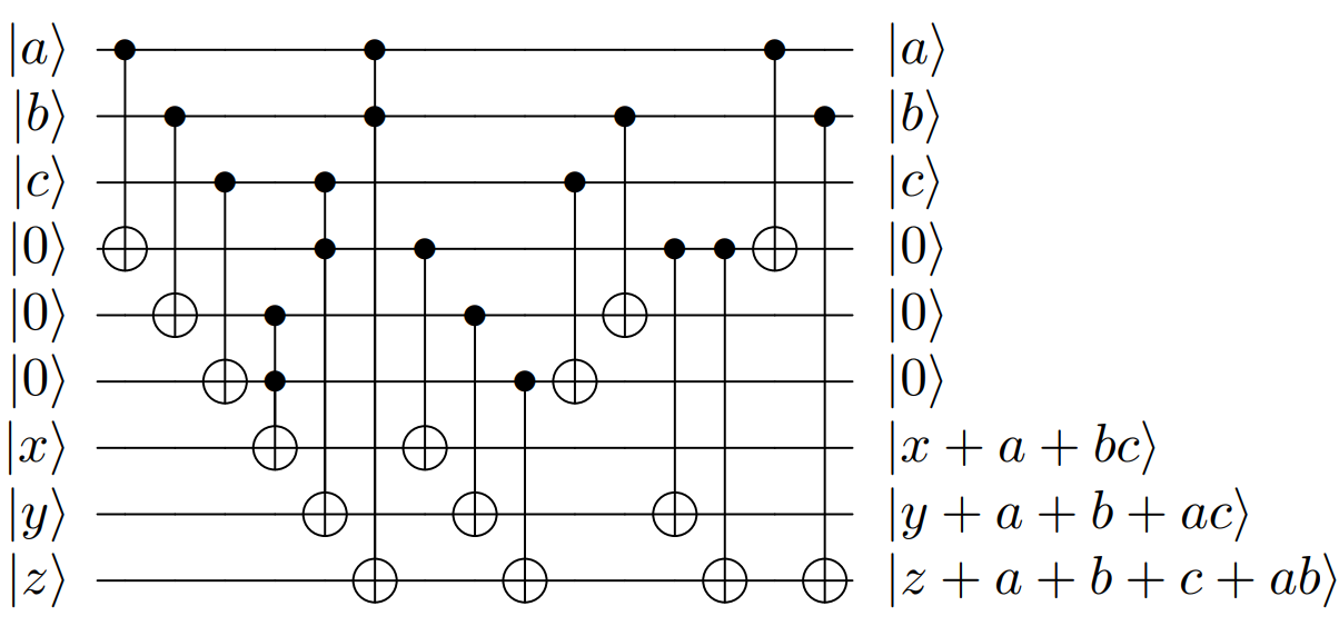
Figure 1: Quantum circuit for computation of one S-Box from LowMC.

The AffineLayer since it is an affine transformation, it consists of a matrix multiplication following by an addition of a constant vector. The details can be seen in [25, Sec. 5.2]. The last function to describe, that is, the KeyExpansion and KeyAddition are only CNOT gates in parallel to perform the addition.

5.3 Costs for running our key recovery algorithm

The costs in terms of gates for running LowMC are similar to those provided in [25]. The only difference for our case is that we will search in a smaller keyspace, that is, the candidates that Algorithm 7 generates in line 9. Table 5 shows the costs for running Grover’s algorithm with the oracle provided in [25]. Furthermore, we select $3$ different sizes of windows for the interval $[B_{min},B_{e})$, namely $e\in\{2^{30},2^{40},2^{50}\}$ full candidates.

Table 5: Total number of gates for running Grover’s algorithm against LowMC.

Value of e	Level	CNOT	1qCliff	T
$30$	L1	$1.78\times 10^{10}$	$1.1\times 10^{8}$	$2.16\times 10^{8}$
	L3	$5.85\times 10^{10}$	$2.42\times 10^{8}$	$3.24\times 10^{8}$
	L5	$1.3\times 10^{11}$	$3.67\times 10^{8}$	$4.11\times 10^{8}$
$40$	L1	$5.68\times 10^{11}$	$3.24\times 10^{9}$	$6.9\times 10^{9}$
	L3	$1.87\times 10^{12}$	$7.74\times 10^{9}$	$1.04\times 10^{10}$
	L5	$4.18\times 10^{12}$	$1.18\times 10^{10}$	$1.31\times 10^{10}$
$50$	L1	$1.82\times 10^{13}$	$1.04\times 10^{11}$	$2.21\times 10^{11}$
	L3	$5.99\times 10^{13}$	$2.48\times 10^{11}$	$3.32\times 10^{11}$
	L5	$1.34\times 10^{14}$	$3.76\times 10^{11}$	$4.21\times 10^{11}$

In our analysis, we need to consider the costs to run $O(N)$ times, since the costs provided in [25] are only for $1$ query. In our case, our costs are $O(N)\times\#CNOT$, $O(N)\times\#1qCliff$, $O(N)\times\#T$, for CNOT, 1qCliff and T gates respectively, where $O(N)$ is taken as $\frac{\pi}{4}\sqrt{2^{e}}$.

Remark 2.

It is possible to run our algorithm in parallel or reuse the circuit. Since we fix the size of window, one can pre-compute the sub-intervals $[B_{0},B_{1}),[B_{1},B_{2}),\ldots,[B_{j},B_{e})$, where each has size $2^{s}$, for $s=0,1,\ldots$. One can reuse the circuit to run each chunk in sequence or run several instances of Grover’s algorithm each one with their chunk of keys.

Remark 3.

Our Algorithm 7 is a “hybrid” algorithm. In our case, we are considering that everything before the Grover’s call is “classical” computation. The same after the call, that is, when we check if the element is found. Hence, we do not need to take into account the costs of the other functions in a quantum computer besides the one in line 11. Furthermore, in our costs, we assume that we always find the element in our search. However, as a future work, we suggest that it is necessary to evaluate the other case, i.e., when the Algorithm 7 will run more than one time.

5.4 Success rate of our key recovery algorithm

In this section, we present the success rate of our key-recovery algorithm for each set of parameters defined for Picnic in [40]. The success rates are estimated by performing simulations of our key recovery algorithm for several selected hyper-parameters.

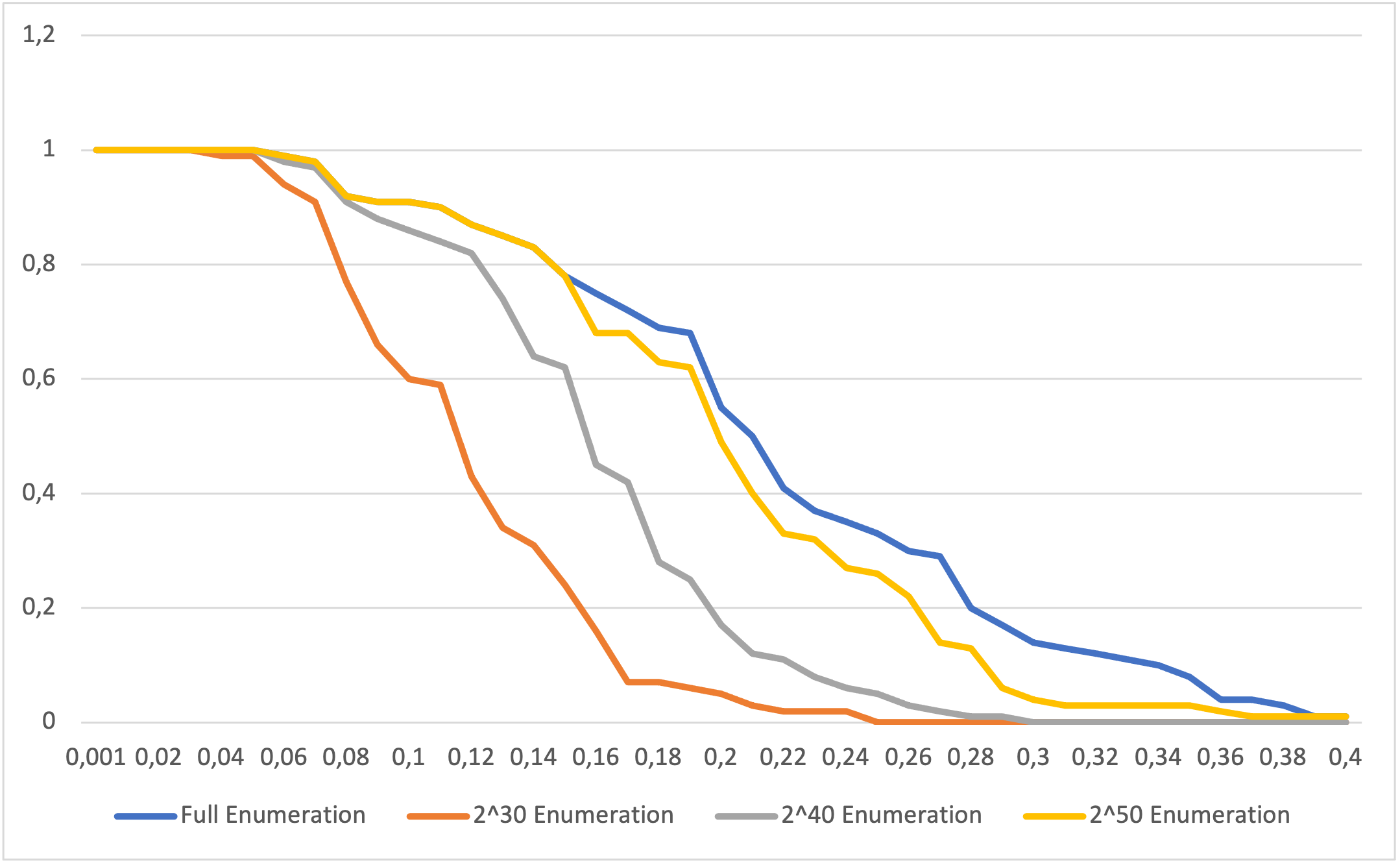
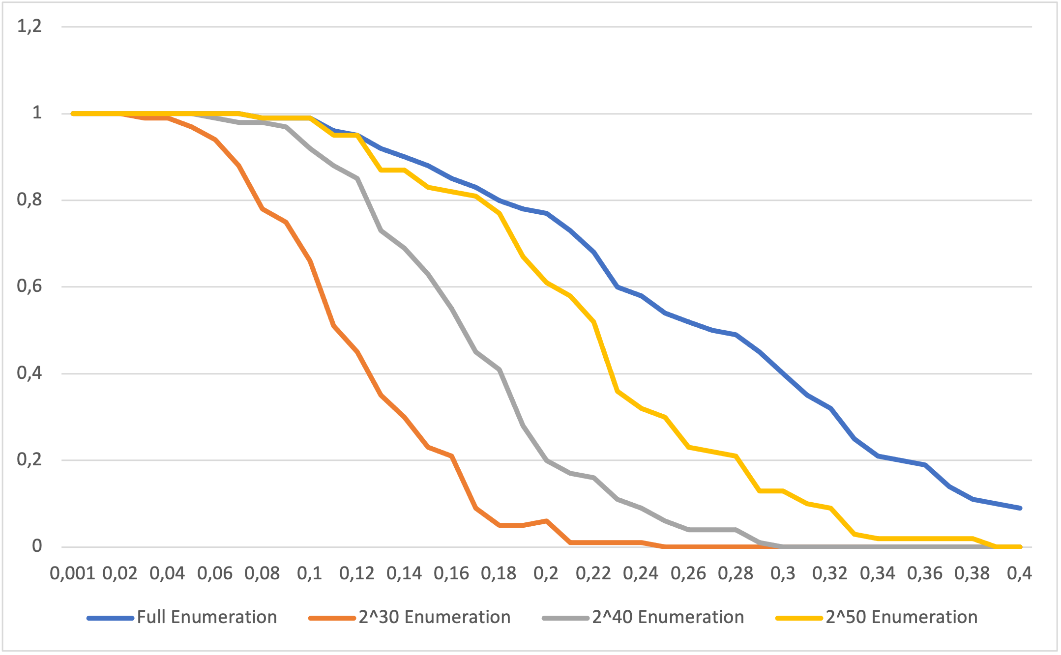
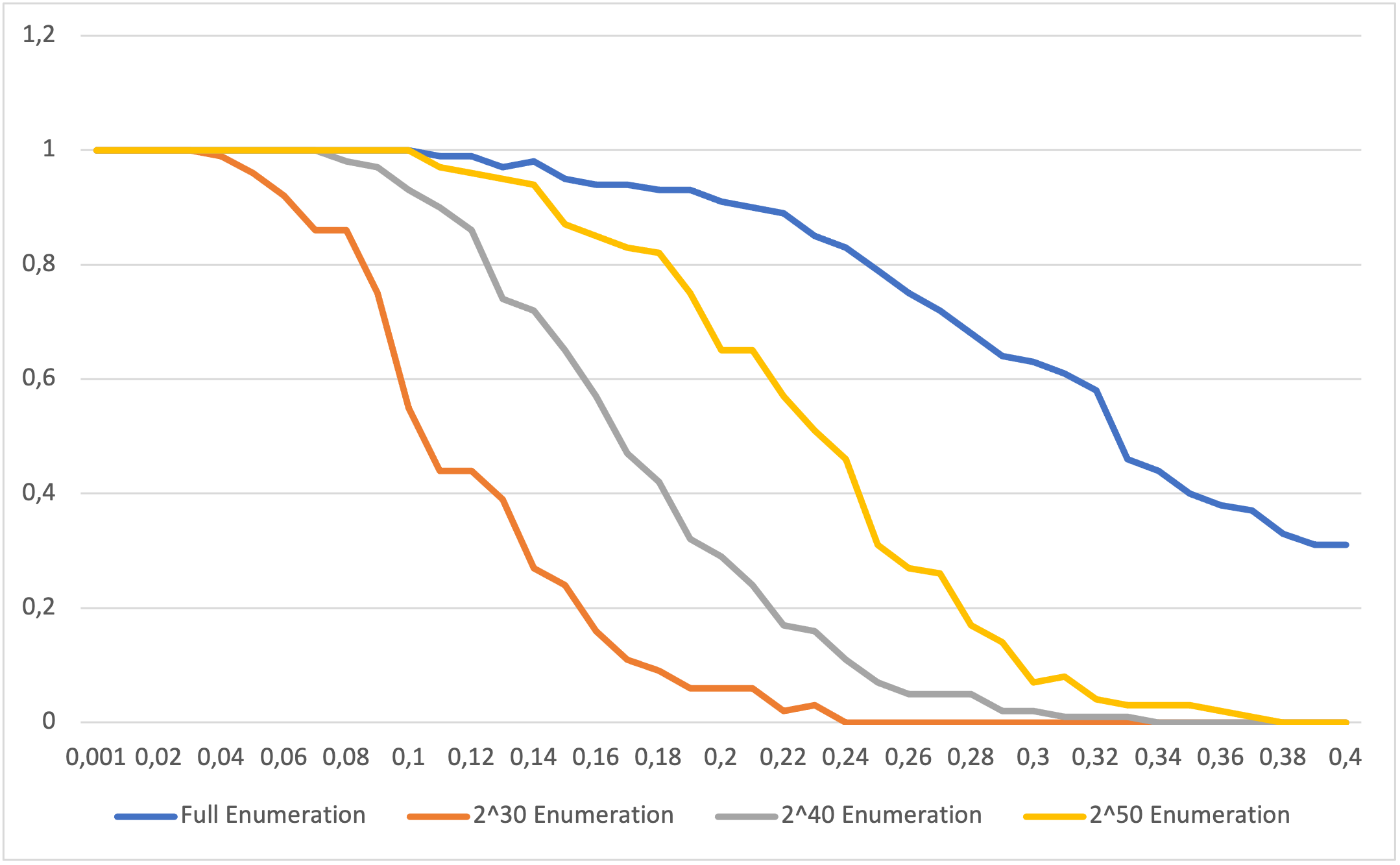
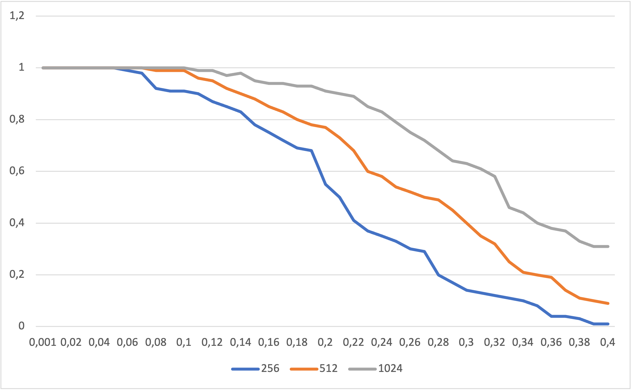
(a) $\mu=256$ (b) $\mu=512$ (c) $\mu=1024$ (d) Full Enumeration for $\mu\in\{256,512,1024\}$ Figure 2: Success rate of our key recovery algorithm with $W=128,w=8,\eta=2$, $\alpha=0.001$ and $\beta\in\{0.001,0.01,0.02,\ldots,0.4\}$ for Picnic parameters picnic-{L1-FS, L1-UR, L1-full} and picnic3-L1. The $x$-axis represents $\beta$, while $y$-axis represents the success rate.

We note that our key-recovery method might find $sk$ from $\widetilde{sk}$, only if each list from the list L returned by Algorithm 2 contains the proper chunk candidates to reconstruct sk. In such a case, a full enumeration of all candidates constructed from the lists of chunk candidates contained in L will find the real private key.

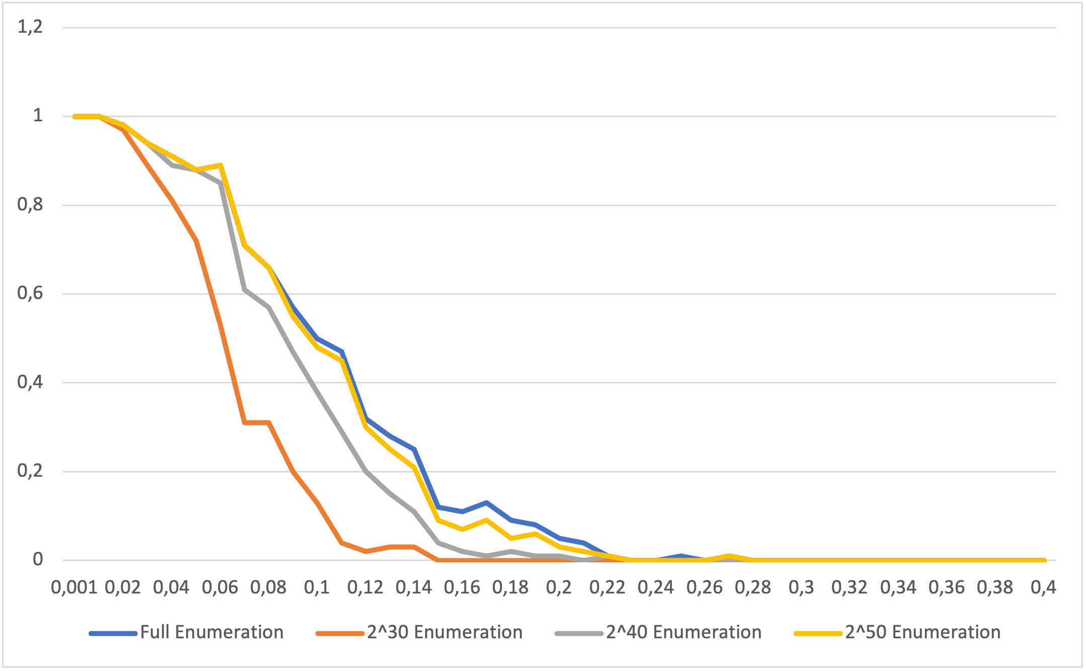
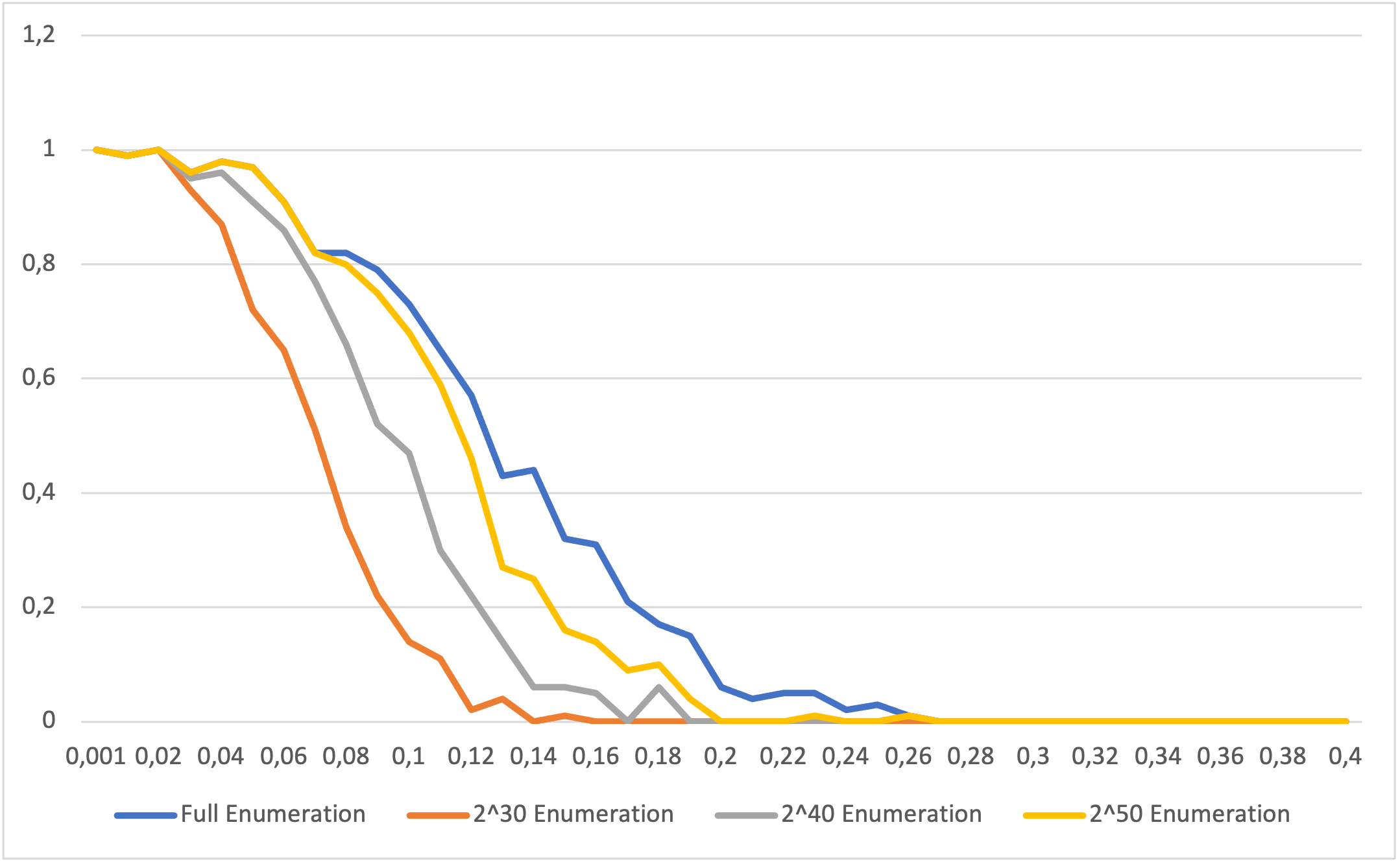
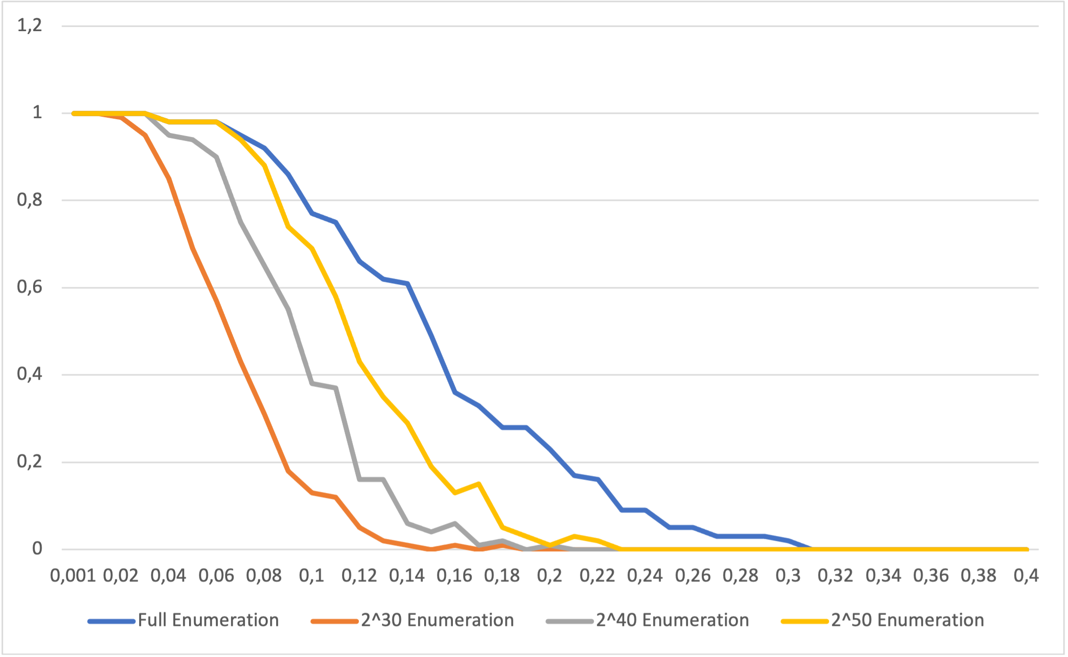
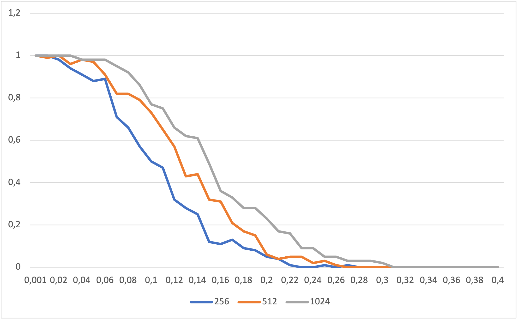
(a) $\mu=256$ (b) $\mu=512$ (c) $\mu=1024$ (d) Full Enumeration for $\mu\in\{256,512,1024\}$

Figure 3: Success rate of our key recovery algorithm with $W=192,w=8,\eta=3$, $\alpha=0.001$ and $\beta\in\{0.001,0.01,0.02,\ldots,0.4\}$ for Picnic parameters picnic-{L3-FS, L3-UR, L3-full} and picnic3-L3. The $x$-axis represents $\beta$, while $y$-axis represents the success rate.

Based on the previous observation, we estimate the success rate of our key-recovery method by assuming the attacker can perform various enumerations from the set of candidates, $\mathcal{C}$, that can be constructed from L. In particular, we assume an attacker is able to enumerate (1) all candidates from $\mathcal{C}$, and (2) the $e$ best high-scoring candidates from $\mathcal{C}$, where $e\in\{2^{30},2^{40},2^{50}\}$ (this is basically what Algorithm 7 does for a given $e$).

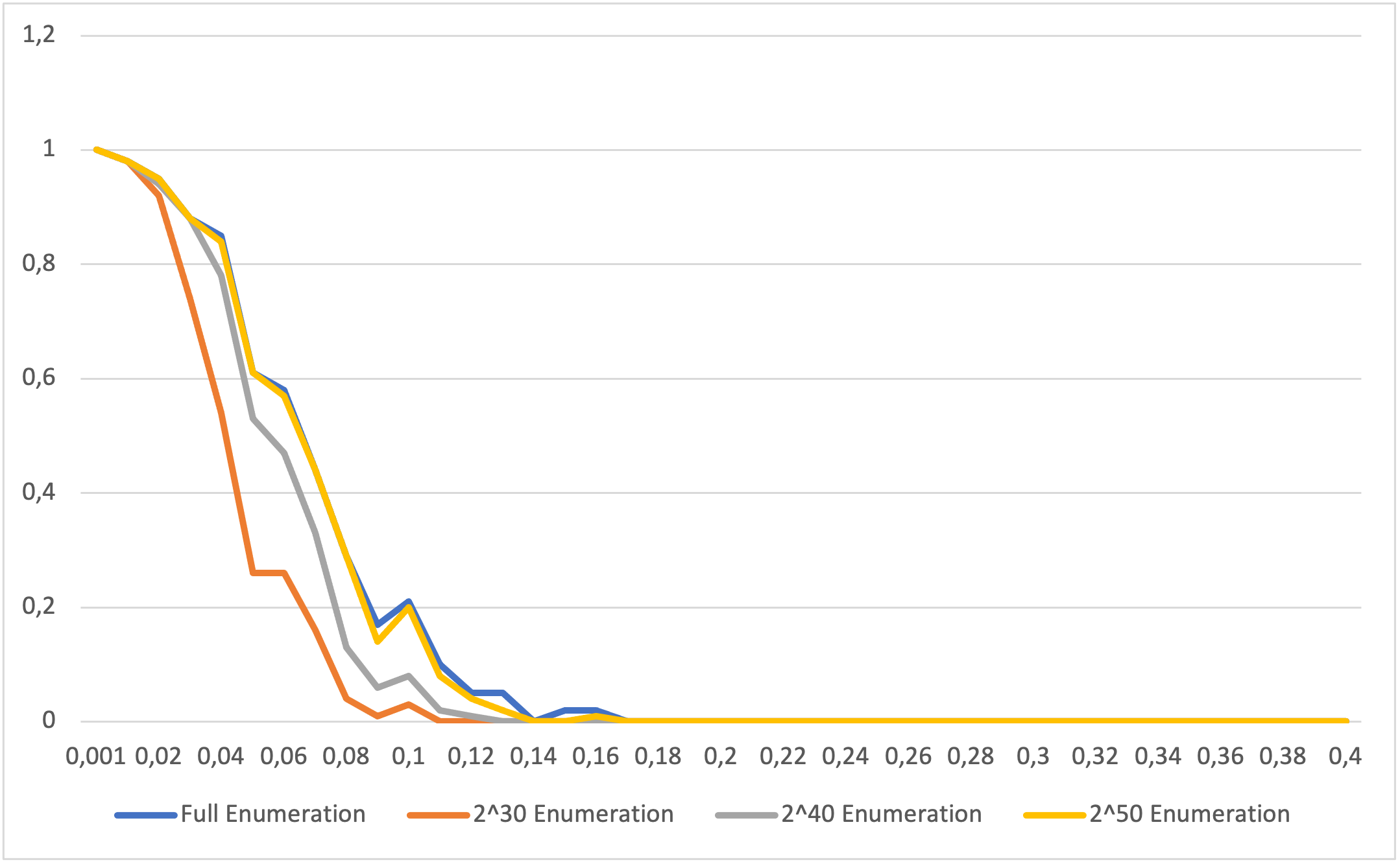
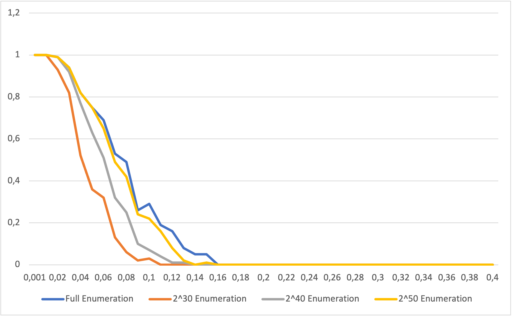
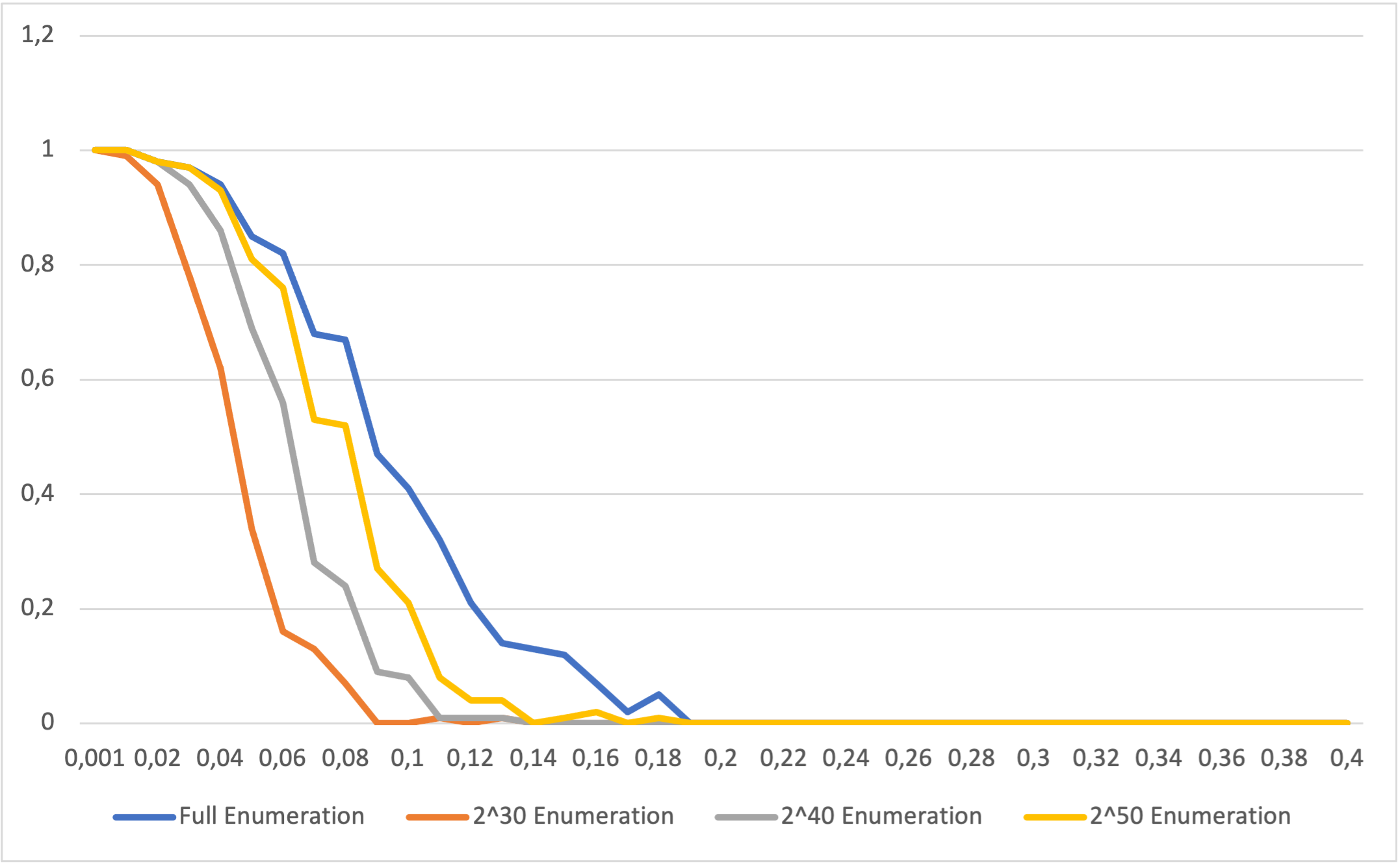
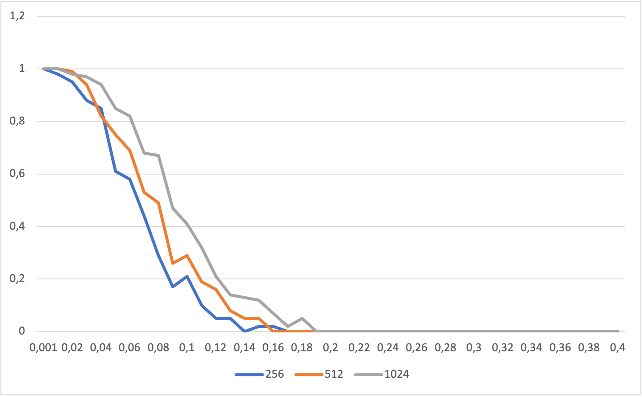
(a) $\mu=256$ (b) $\mu=512$ (c) $\mu=1024$ (d) Full Enumeration for $\mu\in\{256,512,1024\}$

Figure 4: Success rate of our key recovery algorithm with $W=256,w=8,\eta=4$, $\alpha=0.001$ and $\beta\in\{0.001,0.01,0.02,\ldots,0.4\}$ for Picnic parameters picnic-{L5-FS, L5-UR, L5-full} and picnic3-L5. The $x$-axis represents $\beta$, while $y$-axis represents the success rate.

To calculate the success rate of our algorithm for a given $\alpha,\beta$ and a Picnic parameter set P, we perform the following experiment that consists of $100$ trials. In each trial, we first create the key pair $\texttt{sk},\texttt{pk}$ via calling the key generation algorithm from Picnic, as implemented in the Picnic reference implementation [40]. We then perturb sk according to $\alpha,\beta$ to get $\widetilde{sk}$. We then select appropriate values for $W,w,\eta,\mu$, and generate L via calling Algorithm 2 and check if the real key can be reconstructed from L, i.e., by verifying if the corresponding chunk candidates are in the lists of chunk candidates contained in L. If so, that signifies that a full enumeration can recover sk. Otherwise, sk cannot be recovered. Additionally, in case sk can be recovered by a full enumeration, we then calculate three intervals of the form $[B_{min},B_{e})$ for each $e$, as in Algorithm 7, to check if the score of the real private key lies in each of them. Note that this check verifies if performing an enumeration of the $e$ best high-scoring candidates is enough to recover the real private key.

Figure 2 shows the results for the Picnic parameters picnic-{L1-FS, L1-UR, L1-full} and picnic3-L1. In particular, it shows that our key recovery algorithm may find the real private key for $\alpha=0.001$ and $\beta$ in the set $\{0.001,0.01,0.02,\ldots,0.4\}$ when run with the parameters $W=128,w=8,\eta=2$ and $\mu\in\{256,512,1024\}$. Note that the success rate improves as the value of $e$ increases, which is expected. Similarly, Figure 2(d) shows the success rate for the full enumeration improves as the the value of $\mu$ increases, which is also expected. Additionally, note that although the bit length of the private key for the parameters sets picnic-L1-full and picnic3-L1 is $129$ bits, the success rate of our algorithm for these two parameter sets is essentially the same as shown by Figure 2.

Figure 3 shows the results for the Picnic parameters picnic-{L3-FS, L3-UR, L3-full} and picnic3-L3. In particular, it shows that our key recovery algorithm may find the real private key for $\alpha=0.001$ and $\beta$ in the set $\{0.001,0.01,0.02,\ldots,0.3\}$ when run with the parameters $W=192,w=8,\eta=3$ and $\mu\in\{256,512,1024\}$. As mentioned before, the success rate improves as the value of $e$ increases, which is expected. Similarly, Figure 3(d) shows the success rate for the full enumeration improves as the the value of $\mu$ increases, which is also expected.

Figure 4 shows the results for the Picnic parameters picnic-{L5-FS, L5-UR, L5, L5-full} and picnic3-L5. In particular, it shows that our key recovery algorithm may find the real private key for $\alpha=0.001$ and $\beta$ in the set $\{0.001,0.01,0.02,\ldots,0.2\}$ when run with the parameters $W=256,w=8,\eta=4$ and $\mu\in\{256,512,1024\}$. As mentioned before, the success rate improves as the value of $e$ increases, which is expected. Similarly, Figure 4(d) shows the success rate for the full enumeration improves as the the value of $\mu$ increases, which is also expected. Additionally, note that although the bit length of the private key for the parameters sets picnic-L5-full and picnic3-L5 is $255$ bits, the success rate of our algorithm for these two parameter sets is essentially the same as shown by Figure 4.

6 Conclusions

This paper presented a general procedure by which a cold boot attacker may recover a block cipher secret key after procuring a noisy version of the key via a cold boot attack. More specifically, the procedure exploits key enumeration algorithms and a well-known quantum algorithm, namely, Grover’s Algorithm. Also, we showed how to implement the quantum component of our algorithm for several block ciphers such as AES, PRESENT and GIFT,and LowMC. This paper also evaluated Picnic, a post-quantum signature algorithm, in the cold boot attack setting, focusing on its reference implementation. We showed that our key-recovery method effectively reconstructs Picnic private keys for all Picnic parameters for $\alpha=0.001$ and values of $\beta$ in the set $\{0.001,0.01,0.02,\ldots,0.4\}$ (the upper bound for $\beta$ depends on the used parameter set). Additionally, we provided the costs for running our key recovery algorithm by giving the number of quantum gates required to implement it and its running time. As future work, we believe that our key-recovery algorithm may be adapted to tackle key-recovery of other post-quantum algorithms’ private keys in the cold boot attack setting.

References

- [1] Scott Aaronson and Daniel Gottesman. Improved simulation of stabilizer circuits. Physical Review A, 70(5):052328, 2004.
- [2] Scott Aaronson and Daniel Gottesman. Improved simulation of stabilizer circuits. Phys. Rev. A, 70:052328, Nov 2004.
- [3] Martin Albrecht and Carlos Cid. Cold Boot Key Recovery by Solving Polynomial Systems with Noise. In Javier Lopez and Gene Tsudik, editors, Applied Cryptography and Network Security, pages 57–72, Berlin, Heidelberg, 2011. Springer Berlin Heidelberg.
- [4] Martin R. Albrecht, Amit Deo, and Kenneth G. Paterson. Cold Boot Attacks on Ring and Module LWE Keys Under the NTT. IACR Transactions on Cryptographic Hardware and Embedded Systems, 2018(3):173–213, Aug. 2018.
- [5] Martin R. Albrecht, Christian Rechberger, Thomas Schneider, Tyge Tiessen, and Michael Zohner. Ciphers for mpc and fhe. In Elisabeth Oswald and Marc Fischlin, editors, Advances in Cryptology – EUROCRYPT 2015, pages 430–454, Berlin, Heidelberg, 2015. Springer Berlin Heidelberg.
- [6] Martin R. Albrecht, Christian Rechberger, Thomas Schneider, Tyge Tiessen, and Michael Zohner. Ciphers for MPC and FHE. IACR Cryptol. ePrint Arch., 2016:687, 2016.
- [7] Mishal Almazrooie, Azman Samsudin, Rosni Abdullah, and Kussay N. Mutter. Quantum reversible circuit of AES-128. Quantum Information Processing, 17(5):112, Mar 2018.
- [8] Subhadeep Banik, Sumit Kumar Pandey, Thomas Peyrin, Yu Sasaki, Siang Meng Sim, and Yosuke Todo. Gift: A small present. In Wieland Fischer and Naofumi Homma, editors, Cryptographic Hardware and Embedded Systems – CHES 2017, pages 321–345, Cham, 2017. Springer International Publishing.
- [9] Daniel J. Bernstein, Tanja Lange, and Christine van Vredendaal. Tighter, faster, simpler side-channel security evaluations beyond computing power. Cryptology ePrint Archive, Report 2015/221, 2015. http://eprint.iacr.org/2015/221.
- [10] Andrey Bogdanov, Ilya Kizhvatov, Kamran Manzoor, Elmar Tischhauser, and Marc Witteman. Fast and Memory-Efficient Key Recovery in Side-Channel Attacks. In Orr Dunkelman and Liam Keliher, editors, Selected Areas in Cryptography – SAC 2015, pages 310–327, Cham, 2016. Springer International Publishing.
- [11] Marios O. Choudary and P. G. Popescu. Back to massey: Impressively fast, scalable and tight security evaluation tools. In Wieland Fischer and Naofumi Homma, editors, Cryptographic Hardware and Embedded Systems – CHES 2017, pages 367–386, Cham, 2017. Springer International Publishing.
- [12] Marios O. Choudary, Romain Poussier, and François-Xavier Standaert. Score-Based vs. Probability-Based Enumeration – A Cautionary Note. In Orr Dunkelman and Somitra Kumar Sanadhya, editors, Progress in Cryptology – INDOCRYPT 2016, pages 137–152, Cham, 2016. Springer International Publishing.
- [13] Joan Daemen and Vincent Rijmen. The design of rijndael: Aes - the advanced encryption standard (information security and cryptography), 2002.
- [14] James H. Davenport and Benjamin Pring. Improvements to quantum search techniques for Block-Ciphers, with applications to AES. In Orr Dunkelman, Michael J. Jacobson, Jr., and Colin O’Flynn, editors, Selected Areas in Cryptography, pages 360–384, Cham, 2021. Springer International Publishing.
- [15] Liron David and Avishai Wool. A Bounded-Space Near-Optimal Key Enumeration Algorithm for Multi-subkey Side-Channel Attacks. In Helena Handschuh, editor, Topics in Cryptology – CT-RSA 2017, pages 311–327, Cham, 2017. Springer International Publishing.
- [16] Cezary Glowacz, Vincent Grosso, Romain Poussier, Joachim Schüth, and François-Xavier Standaert. Simpler and more efficient rank estimation for side-channel security assessment. In Gregor Leander, editor, Fast Software Encryption, pages 117–129, Berlin, Heidelberg, 2015. Springer Berlin Heidelberg.
- [17] Markus Grassl, Brandon Langenberg, Martin Roetteler, and Rainer Steinwandt. Applying Grover’s algorithm to AES: quantum resource estimates. In Post-Quantum Cryptography – 7th International Workshop, PQCrypto 2016, Fukuoka, Japan, February 24-26, 2016, Proceedings, pages 29–43, 2016.
- [18] Vincent Grosso. Scalable key rank estimation (and key enumeration) algorithm for large keys. In Begül Bilgin and Jean-Bernard Fischer, editors, Smart Card Research and Advanced Applications, pages 80–94, Cham, 2019. Springer International Publishing.
- [19] Lov K. Grover. A fast quantum mechanical algorithm for database search. In Proceedings of the Twenty-Eighth Annual ACM Symposium on the Theory of Computing, Philadelphia, Pennsylvania, USA, May 22-24, 1996, pages 212–219, 1996.
- [20] J. Alex Halderman, Seth D. Schoen, Nadia Heninger, William Clarkson, William Paul, Joseph A. Calandrino, Ariel J. Feldman, Jacob Appelbaum, and Edward W. Felten. Lest we remember: Cold-boot attacks on encryption keys. Commun. ACM, 52(5):91–98, May 2009.
- [21] Wilko Henecka, Alexander May, and Alexander Meurer. Correcting Errors in RSA Private Keys. In Tal Rabin, editor, Advances in Cryptology – CRYPTO 2010, pages 351–369, Berlin, Heidelberg, 2010. Springer Berlin Heidelberg.
- [22] Nadia Heninger and Hovav Shacham. Reconstructing RSA Private Keys from Random Key Bits. In Shai Halevi, editor, Advances in Cryptology - CRYPTO 2009, pages 1–17, Berlin, Heidelberg, 2009. Springer Berlin Heidelberg.
- [23] Zhenyu Huang and Dongdai Lin. A new method for solving polynomial systems with noise over and its applications in cold boot key recovery. In Lars R. Knudsen and Huapeng Wu, editors, Selected Areas in Cryptography, pages 16–33, Berlin, Heidelberg, 2013. Springer Berlin Heidelberg.
- [24] Kyungbae Jang, Gyeongju Song, Hyunjun Kim, Hyeokdong Kwon, Hyunji Kim, and Hwajeong Seo. Efficient implementation of PRESENT and GIFT on quantum computers. Applied Sciences, 11(11), 2021.
- [25] Samuel Jaques, Michael Naehrig, Martin Roetteler, and Fernando Virdia. Implementing grover oracles for quantum key search on aes and lowmc. In Anne Canteaut and Yuval Ishai, editors, Advances in Cryptology – EUROCRYPT 2020, pages 280–310, Cham, 2020. Springer International Publishing.
- [26] Abdel Alim Kamal and Amr M. Youssef. Applications of SAT Solvers to AES Key Recovery from Decayed Key Schedule Images. In 2010 Fourth International Conference on Emerging Security Information, Systems and Technologies, pages 216–220, 2010.
- [27] Panjin Kim, Daewan Han, and Kyung Chul Jeong. Time–space complexity of quantum search algorithms in symmetric cryptanalysis: applying to aes and sha-2. Quantum Information Processing, 17(12):339, Oct 2018.
- [28] Brandon Langenberg, Hai Pham, and Rainer Steinwandt. Reducing the cost of implementing the advanced encryption standard as a quantum circuit. IEEE Transactions on Quantum Engineering, 1:1–12, 2020.
- [29] Hyung Tae Lee, HongTae Kim, Yoo-Jin Baek, and Jung Hee Cheon. Correcting Errors in Private Keys Obtained from Cold Boot Attacks. In Howon Kim, editor, Information Security and Cryptology - ICISC 2011, pages 74–87, Berlin, Heidelberg, 2012. Springer Berlin Heidelberg.
- [30] Simon Lindenlauf, Hans Höfken, and Marko Schuba. Cold boot attacks on DDR2 and DDR3 SDRAM. In 2015 10th International Conference on Availability, Reliability and Security, pages 287–292, 2015.
- [31] Jake Longo, Daniel P. Martin, Luke Mather, Elisabeth Oswald, Benjamin Sach, and Martijn Stam. How low can you go? Using side-channel data to enhance brute-force key recovery. Cryptology ePrint Archive, Report 2016/609, 2016. http://eprint.iacr.org/2016/609.
- [32] Daniel P. Martin, Luke Mather, Elisabeth Oswald, and Martijn Stam. Characterisation and estimation of the key rank distribution in the context of side channel evaluations. In Jung Hee Cheon and Tsuyoshi Takagi, editors, Advances in Cryptology – ASIACRYPT 2016, pages 548–572, Berlin, Heidelberg, 2016. Springer Berlin Heidelberg.
- [33] Daniel P. Martin, Ashley Montanaro, Elisabeth Oswald, and Dan Shepherd. Quantum key search with side channel advice. In Carlisle Adams and Jan Camenisch, editors, Selected Areas in Cryptography – SAC 2017, pages 407–422, Cham, 2018. Springer International Publishing.
- [34] Daniel P. Martin, Jonathan F. O’Connell, Elisabeth Oswald, and Martijn Stam. Counting keys in parallel after a side channel attack. In Tetsu Iwata and Jung Hee Cheon, editors, Advances in Cryptology – ASIACRYPT 2015, pages 313–337, Berlin, Heidelberg, 2015. Springer Berlin Heidelberg.
- [35] Kenneth G. Paterson, Antigoni Polychroniadou, and Dale L. Sibborn. A Coding-Theoretic Approach to Recovering Noisy RSA Keys. In Xiaoyun Wang and Kazue Sako, editors, Advances in Cryptology – ASIACRYPT 2012, pages 386–403, Berlin, Heidelberg, 2012. Springer Berlin Heidelberg.
- [36] Kenneth G. Paterson and Ricardo Villanueva-Polanco. Cold boot attacks on NTRU. In Arpita Patra and Nigel P. Smart, editors, Progress in Cryptology – INDOCRYPT 2017, pages 107–125, Cham, 2017. Springer International Publishing.
- [37] Bertram Poettering and Dale L. Sibborn. Cold Boot Attacks in the Discrete Logarithm Setting. In Kaisa Nyberg, editor, Topics in Cryptology — CT-RSA 2015, pages 449–465, Cham, 2015. Springer International Publishing.
- [38] Romain Poussier, Vincent Grosso, and François-Xavier Standaert. Comparing approaches to rank estimation for side-channel security evaluations. In Naofumi Homma and Marcel Medwed, editors, Smart Card Research and Advanced Applications, pages 125–142, Cham, 2016. Springer International Publishing.
- [39] Romain Poussier, François-Xavier Standaert, and Vincent Grosso. Simple key enumeration (and rank estimation) using histograms: An integrated approach. In Benedikt Gierlichs and Axel Y. Poschmann, editors, Cryptographic Hardware and Embedded Systems – CHES 2016, pages 61–81, Berlin, Heidelberg, 2016. Springer Berlin Heidelberg.
- [40] Picnic Team. Picnic A Family of Post-Quantum Secure Digital Signature Algorithms, 2020. https://github.com/Microsoft/Picnic.
- [41] Nicolas Veyrat-Charvillon, Benoît Gérard, Mathieu Renauld, and François-Xavier Standaert. An optimal key enumeration algorithm and its application to side-channel attacks. In Lars R. Knudsen and Huapeng Wu, editors, Selected Areas in Cryptography, pages 390–406, Berlin, Heidelberg, 2013. Springer Berlin Heidelberg.
- [42] Nicolas Veyrat-Charvillon, Benoît Gérard, and François-Xavier Standaert. Security evaluations beyond computing power. In Thomas Johansson and Phong Q. Nguyen, editors, Advances in Cryptology – EUROCRYPT 2013, pages 126–141, Berlin, Heidelberg, 2013. Springer Berlin Heidelberg.
- [43] Ricardo Villanueva-Polanco. Cold boot attacks on Bliss. In Peter Schwabe and Nicolas Thériault, editors, Progress in Cryptology – LATINCRYPT 2019, pages 40–61, Cham, 2019. Springer International Publishing.
- [44] Ricardo Villanueva Polanco. Cold Boot Attacks on Post-Quantum Schemes. PhD thesis, Royal Holloway, University of London, March 2019.
- [45] Ricardo Villanueva-Polanco. A Comprehensive Study of the Key Enumeration Problem. Entropy, 21(10), 2019.
- [46] Ricardo Villanueva-Polanco. Cold boot attacks on LUOV. Applied Sciences, 10(12), 2020.
- [47] Ricardo Villanueva-Polanco and Eduardo Angulo-Madrid. Cold Boot Attacks on the Supersingular Isogeny Key Encapsulation (SIKE) Mechanism. Applied Sciences, 11(1), 2021.
- [48] Yoo-Seung Won, Jong-Yeon Park, Dong-Guk Han, and Shivam Bhasin. Practical cold boot attack on IoT device - case study on Raspberry Pi -. In 2020 IEEE International Symposium on the Physical and Failure Analysis of Integrated Circuits (IPFA), pages 1–4, 2020.
- [49] Gangqiang Yang, Bo Zhu, Valentin Suder, Mark D. Aagaard, and Guang Gong. The simeck family of lightweight block ciphers. Cryptology ePrint Archive, Report 2015/612, 2015. https://ia.cr/2015/612.
- [50] Noson S Yanofsky and Mirco A Mannucci. Quantum computing for computer scientists. Cambridge University Press, 2008.
- [51] Xin Ye, Thomas Eisenbarth, and William Martin. Bounded, yet sufficient? how to determine whether limited side channel information enables key recovery. In Marc Joye and Amir Moradi, editors, Smart Card Research and Advanced Applications, pages 215–232, Cham, 2015. Springer International Publishing.