EF-BV: A Unified Theory of Error Feedback and Variance Reduction Mechanisms for Biased and Unbiased Compression in Distributed Optimization

Abstract

In distributed or federated optimization and learning, communication between the different computing units is often the bottleneck and gradient compression is widely used to reduce the number of bits sent within each communication round of iterative methods. There are two classes of compression operators and separate algorithms making use of them. In the case of unbiased random compressors with bounded variance (e.g., rand-k), the DIANA algorithm of Mishchenko et al. (2019), which implements a variance reduction technique for handling the variance introduced by compression, is the current state of the art. In the case of biased and contractive compressors (e.g., top-k), the EF21 algorithm of Richtárik et al. (2021), which instead implements an error-feedback mechanism, is the current state of the art. These two classes of compression schemes and algorithms are distinct, with different analyses and proof techniques. In this paper, we unify them into a single framework and propose a new algorithm, recovering DIANA and EF21 as particular cases. Our general approach works with a new, larger class of compressors, which has two parameters, the bias and the variance, and includes unbiased and biased compressors as particular cases. This allows us to inherit the best of the two worlds: like EF21 and unlike DIANA, biased compressors, like top-k, whose good performance in practice is recognized, can be used. And like DIANA and unlike EF21, independent randomness at the compressors allows to mitigate the effects of compression, with the convergence rate improving when the number of parallel workers is large. This is the first time that an algorithm with all these features is proposed. We prove its linear convergence under certain conditions. Our approach takes a step towards better understanding of two so-far distinct worlds of communication-efficient distributed learning.

1 Introduction

In the big data era, the explosion in size and complexity of the data arises in parallel to a shift towards distributed computations (Verbraeken et al., 2021), as modern hardware increasingly relies on the power of uniting many parallel units into one system. For distributed optimization and learning tasks, specific issues arise, such as decentralized data storage. In the modern paradigm of federated learning (Konečný et al., 2016; McMahan et al., 2017; Kairouz et al., 2021; Li et al., 2020a), a potentially huge number of devices, with their owners’ data stored on each of them, are involved in the collaborative process of training a global machine learning model. The goal is to exploit the wealth of useful information lying in the heterogeneous data stored across the network of such devices. But users are increasingly sensitive to privacy concerns and prefer their data to never leave their devices. Thus, the devices have to communicate the right amount of information back and forth with a distant server, for this distributed learning process to work. Communication, which can be costly and slow, is the main bottleneck in this framework. So, it is of primary importance to devise novel algorithmic strategies, which are efficient in terms of computation and communication complexities. A natural and widely used idea is to make use of (lossy) compression, to reduce the size of the communicated messages (Alistarh et al., 2017; Wen et al., 2017; Wangni et al., 2018; Khaled & Richtárik, 2019; Albasyoni et al., 2020; Basu et al., 2020; Dutta et al., 2020; Sattler et al., 2020; Xu et al., 2021).

In this paper, we propose a stochastic gradient descent (SGD)-type method for distributed optimization, which uses possibly biased and randomized compression operators. Our algorithm is variance-reduced (Hanzely & Richtárik, 2019; Gorbunov et al., 2020a; Gower et al., 2020); that is, it converges to the exact solution, with fixed stepsizes, without any restrictive assumption on the functions to minimize.

Problem.   We consider the convex optimization problem

$$\operatorname*{\mathrm{minimize}}_{x\in\mathbb{R}^{d}}\;\underbrace{\frac{1}{n}\sum_{i=1}^{n}f_{i}(x)}_{f(x)}+R(x),$$ (1)

where $d\geq 1$ is the model dimension; $R:\mathbb{R}^{d}\rightarrow\mathbb{R}\cup\{+\infty\}$ is a proper, closed, convex function (Bauschke & Combettes, 2017), whose proximity operator $\mathrm{prox}_{\gamma R}:x\mapsto\operatorname*{arg\,min}_{y\in\mathbb{R}^{d}}\big{(}\gamma R(y)+\frac{1}{2}\|x-y\|^{2}\big{)}$ is easy to compute, for any $\gamma>0$ (Parikh & Boyd, 2014; Condat et al., 2022a, b); $n\geq 1$ is the number of functions; each function $f_{i}:\mathbb{R}^{d}\rightarrow\mathbb{R}$ is convex and $L_{i}$-smooth, for some $L_{i}>0$; that is, $f_{i}$ is differentiable on $\mathbb{R}^{d}$ and its gradient $\nabla f_{i}$ is $L_{i}$-Lipschitz continuous: for every $x\in\mathbb{R}^{d}$ and $x^{\prime}\in\mathbb{R}^{d}$, $\|\nabla f_{i}(x)-\nabla f_{i}(x^{\prime})\|\leq L_{i}\|x-x^{\prime}\|$.

We set $L_{\max}\coloneqq\max_{i}L_{i}$ and $\tilde{L}\coloneqq\sqrt{\frac{1}{n}\sum_{i=1}^{n}L_{i}^{2}}$. The average function $f\coloneqq\frac{1}{n}\sum_{i=1}^{n}f_{i}$ is $L$-smooth, for some $L\leq\tilde{L}\leq L_{\max}$. A minimizer of $f+R$ is supposed to exist. For any integer $m\geq 1$, we define the set $\mathcal{I}_{m}\coloneqq\{1,\ldots,m\}$.

Algorithms and Prior Work.   Distributed proximal SGD solves the problem (1) by iterating $x^{t+1}\coloneqq\mathrm{prox}_{\gamma R}\big{(}x^{t}-\frac{\gamma}{n}\sum_{i=1}^{n}g_{i}^{t}\big{)}$, where $\gamma$ is a stepsize and the vectors $g_{i}^{t}$ are possibly stochastic estimates of the gradients $\nabla f_{i}(x^{t})$, which are cheap to compute or communicate. Compression is typically performed by the application of a possibly randomized operator $\mathcal{C}:\mathbb{R}^{d}\rightarrow\mathbb{R}^{d}$; that is, for any $x$, $\mathcal{C}(x)$ denotes a realization of a random variable, whose probability distribution depends on $x$. Compressors have the property that it is much easier/faster to transfer $\mathcal{C}(x)$ than the original message $x$. This can be achieved in several ways, for instance by sparsifying the input vector (Alistarh et al., 2018), or by quantizing its entries (Alistarh et al., 2017; Horváth et al., 2019; Gandikota et al., 2019; Mayekar & Tyagi, 2021; Saha et al., 2021), or via a combination of these and other approaches (Horváth et al., 2019; Albasyoni et al., 2020; Beznosikov et al., 2020). There are two classes of compression operators often studied in the literature: 1) unbiased compression operators, satisfying a variance bound proportional to the squared norm of the input vector, and 2) biased compression operators, whose square distortion is contractive with respect to the squared norm of the input vector; we present these two classes in Sections 2.1 and 2.2, respectively.

Prior work: DIANA with unbiased compressors.  An important contribution to the field in the recent years is the variance-reduced SGD-type method called DIANA (Mishchenko et al., 2019), which uses unbiased compressors; it is shown in Fig. 1. DIANA was analyzed and extended in several ways, including bidirectional compression and acceleration, see, e.g., the work of Horváth et al. (2022); Mishchenko et al. (2020); Condat & Richtárik (2022); Philippenko & Dieuleveut (2020); Li et al. (2020b); Gorbunov et al. (2020b), and Gorbunov et al. (2020a); Khaled et al. (2020) for general theories about SGD-type methods, including variants using unbiased compression of (stochastic) gradients.

Prior work: Error feedback with biased contractive compressors.  Our understanding of distributed optimization using biased compressors is more limited. The key complication comes from the fact that their naive use within methods like gradient descent can lead to divergence, as widely observed in practice, see also Example 1 of Beznosikov et al. (2020). Error feedback (EF), also called error compensation, techniques were proposed to fix this issue and obtain convergence, initially as heuristics (Seide et al., 2014). Theoretical advances have been made in the recent years in the analysis of EF, see the discussions and references in Richtárik et al. (2021) and Lin et al. (2022). But the question of whether it is possible to obtain a linearly convergent EF method in the general heterogeneous data setting, relying on biased compressors only, was still an open problem; until last year, 2021, when Richtárik et al. (2021) re-engineered the classical EF mechanism and came up with a new algorithm, called EF21. It was then extended in several ways, including by considering server-side compression, and the support of a regularizer $R$ in (1), by Fatkhullin et al. (2021). EF21 is shown in Fig. 1.

Motivation and challenge.  While EF21 resolved an important theoretical problem in the field of distributed optimization with contractive compression, there are still several open questions. In particular, DIANA with independent random compressors has a $\frac{1}{n}$ factor in its iteration complexity; that is, it converges faster when the number $n$ of workers is larger. EF21 does not have this property: its convergence rate does not depend on $n$. Also, the convergence analysis and proof techniques for the two algorithms are different: the linear convergence analysis of DIANA relies on $\|x^{t}-x^{\star}\|^{2}$ and $\|h_{i}^{t}-\nabla f_{i}(x^{\star})\|^{2}$ tending to zero, where $x^{t}$ is the estimate of the solution $x^{\star}$ at iteration $t$ and $h_{i}^{t}$ is the control variate maintained at node $i$, whereas the analysis of EF21 relies on $(f+R)(x^{t})-(f+R)(x^{\star})$ and $\|h_{i}^{t}-\nabla f_{i}(x^{t})\|^{2}$ tending to zero, and under different assumptions. This work aims at filling this gap. That is, we want to address the following open problem:

Table 1: Desirable properties of a distributed compressed gradient descent algorithm converging to an exact solution of (1) and whether they are satisfied by the state-of-the-art algorithms DIANA and EF21 and their currently-known analysis, and the proposed algorithm EF-BV.

	DIANA	EF21	EF-BV
handles unbiased compressors in $\mathbb{U}(\omega)$ for any $\omega\geq 0$	✓	✓1	✓
handles biased contractive compressors in $\mathbb{B}(\alpha)$ for any $\alpha\in(0,1]$	✗	✓	✓
handles compressors in $\mathbb{C}(\eta,\omega)$ for any $\eta\in[0,1)$, $\omega\geq 0$	✗	✓1	✓
recovers DIANA and EF21 as particular cases	✗	✗	✓
the convergence rate improves when $n$ is large	✓	✗	✓

¹: with pre-scaling with $\lambda<1$, so that $\mathcal{C}^{\prime}=\lambda\mathcal{C}\in\mathbb{B}(\alpha)$ is used instead of $\mathcal{C}$

Is it possible to design an algorithm, which combines the advantages of DIANA and EF21? That is, such that:

1. It deals with unbiased compressors, biased contractive compressors, and possibly even more.

2. It recovers DIANA and EF21 as particular cases.

3. Its convergence rate improves with $n$ large.

Contributions.  We answer positively this question and propose a new algorithm, which we name EF-BV, for Error Feedback with Bias-Variance decomposition, which for the first time satisfies the three aforementioned properties. This is illustrated in Tab. 1. More precisely, our contributions are:

1. We propose a new, larger class of compressors, which includes unbiased and biased contractive compressors as particular cases, and has two parameters, the bias $\eta$ and the variance $\omega$. A third parameter $\omega_{\mathrm{av}}$ describes the resulting variance from the parallel compressors after aggregation, and is key to getting faster convergence with large $n$, by allowing larger stepsizes than in EF21 in our framework.

2. We propose a new algorithm, named EF-BV, which exploits the properties of the compressors in the new class using two scaling parameters $\lambda$ and $\nu$. For particular values of $\lambda$ and $\nu$, EF21 and DIANA are recovered as particular cases. But by setting the values of $\lambda$ and $\nu$ optimally with respect to $\eta$, $\omega$, $\omega_{\mathrm{av}}$ in EF-BV, faster convergence can be obtained.

3. We prove linear convergence of EF-BV under a Kurdyka–Łojasiewicz condition of $f+R$, which is weaker than strong convexity of $f+R$. Even for EF21 and DIANA, this is new.

4. We provide new insights on EF21 and DIANA; for instance, we prove linear convergence of DIANA with biased compressors.

2 Compressors and their properties

2.1 Unbiased compressors

For every $\omega\geq 0$, we introduce the set $\mathbb{U}(\omega)$ of unbiased compressors, which are randomized operators of the form $\mathcal{C}:\mathbb{R}^{d}\rightarrow\mathbb{R}^{d}$, satisfying

$$\mathbb{E}[\mathcal{C}(x)]=x\quad\mbox{and}\quad\mathbb{E}[\|\mathcal{C}(x)-x\|^{2}]\leq\omega\|x\|^{2},\quad\forall x\in\mathbb{R}^{d},$$ (2)

where $\mathbb{E}\!\left[\cdot\right]$ denotes the expectation. The smaller $\omega$, the better, and $\omega=0$ if and only if $\mathcal{C}=\mathrm{Id}$, the identity operator, which does not compress. We can remark that if $\mathcal{C}\in\mathbb{U}(\omega)$ is deterministic, then $\mathcal{C}=\mathrm{Id}$. So, unbiased compressors are random ones. A classical unbiased compressor is rand-$k$, for some $k\in\mathcal{I}_{d}$, which keeps $k$ elements chosen uniformly at random, multiplied by $\frac{d}{k}$, and sets the other elements to 0. It is easy to see that rand-$k$ belongs to $\mathbb{U}(\omega)$ with $\omega=\frac{d}{k}-1$ (Beznosikov et al., 2020).

2.2 Biased contractive compressors

For every $\alpha\in(0,1]$, we introduce the set $\mathbb{B}(\alpha)$ of biased contractive compressors, which are possibly randomized operators of the form $\mathcal{C}:\mathbb{R}^{d}\rightarrow\mathbb{R}^{d}$, satisfying

$$\mathbb{E}[\|\mathcal{C}(x)-x\|^{2}]\leq(1-\alpha)\|x\|^{2},\quad\forall x\in\mathbb{R}^{d}.$$ (3)

We use the term ‘contractive’ to reflect the fact that the squared norm in the left hand side of (3) is smaller, in expectation, than the one in the right hand side, since $1-\alpha<1$. This is not the case in (2), where $\omega$ can be arbitrarily large. The larger $\alpha$, the better, and $\alpha=1$ if and only if $\mathcal{C}=\mathrm{Id}$. Biased compressors need not be random: a classical biased and deterministic compressor is top-$k$, for some $k\in\mathcal{I}_{d}$, which keeps the $k$ elements with largest absolute values unchanged and sets the other elements to 0. It is easy to see that top-$k$ belongs to $\mathbb{B}(\alpha)$ with $\alpha=\frac{k}{d}$ (Beznosikov et al., 2020).

2.3 New general class of compressors

We refer to Beznosikov et al. (2020), Table 1 in Safaryan et al. (2021), Zhang et al. (2021), Szlendak et al. (2022), for examples of compressors in $\mathbb{U}(\omega)$ or $\mathbb{B}(\alpha)$, and to Xu et al. (2020) for a system-oriented survey.

In this work, we introduce a new, more general class of compressors, ruled by 2 parameters, to allow for a finer characterization of their properties. Indeed, with any compressor $\mathcal{C}$, we can do a bias-variance decomposition of the compression error: for every $x\in\mathbb{R}^{d}$,

$$\mathbb{E}\big{[}\|\mathcal{C}(x)-x\|^{2}\big{]}={\underbrace{\big{\|}\mathbb{E}[\mathcal{C}(x)]-x\big{\|}}_{\text{bias}}}^{2}+\underbrace{\mathbb{E}\Big{[}\big{\|}\mathcal{C}(x)-\mathbb{E}[\mathcal{C}(x)]\big{\|}^{2}\Big{]}}_{\text{variance}}.$$ (4)

Therefore, to better characterize the properties of compressors, we propose to parameterize these two parts, instead of only their sum: for every $\eta\in[0,1)$ and $\omega\geq 0$, we introduce the new class $\mathbb{C}(\eta,\omega)$ of possibly random and biased operators, which are randomized operators of the form $\mathcal{C}:\mathbb{R}^{d}\rightarrow\mathbb{R}^{d}$, satisfying, for every $x\in\mathbb{R}^{d}$, the two properties:

$$\mathrm{(i)}\quad \big{\|}\mathbb{E}[\mathcal{C}(x)]-x\big{\|}\leq\eta\|x\|,$$

$$\mathrm{(ii)}\quad \mathbb{E}\Big{[}\big{\|}\mathcal{C}(x)-\mathbb{E}[\mathcal{C}(x)]\big{\|}^{2}\Big{]}\leq\omega\|x\|^{2}.$$

Thus, $\eta$ and $\omega$ control the relative bias and variance of the compressor, respectively. Note that $\omega$ can be arbitrarily large, but the compressors will be scaled in order to control the compression error, as we discuss in Sect. (2.5). On the other hand, we must have $\eta<1$, since otherwise, no scaling can keep the compressor’s discrepancy under control.

We have the following properties:

1. $\mathbb{C}(\eta,0)$ is the class of deterministic compressors in $\mathbb{B}(\alpha)$, with $1-\alpha=\eta^{2}$.

2. $\mathbb{C}(0,\omega)=\mathbb{U}(\omega)$, for every $\omega\geq 0$. In words, if its bias $\eta$ is zero, the compressor is unbiased with relative variance $\omega$.

3. Because of the bias-variance decomposition (4), if $\mathcal{C}\in\mathbb{C}(\eta,\omega)$ with $\eta^{2}+\omega<1$, then $\mathcal{C}\in\mathbb{B}(\alpha)$ with

   $$1-\alpha=\eta^{2}+\omega.$$ (5)

4. Conversely, if $\mathcal{C}\in\mathbb{B}(\alpha)$, one easily sees from (4) that there exist $\eta\leq\sqrt{1-\alpha}$ and $\omega\leq 1-\alpha$ such that $\mathcal{C}\in\mathbb{C}(\eta,\omega)$.

Thus, the new class $\mathbb{C}(\eta,\omega)$ generalizes the two previously known classes $\mathbb{U}(\omega)$ and $\mathbb{B}(\alpha)$. Actually, for compressors in $\mathbb{U}(\omega)$ and $\mathbb{B}(\alpha)$, we can just use DIANA and EF21, and our proposed algorithm EF-BV will stand out when the compressors are neither in $\mathbb{U}(\omega)$ nor in $\mathbb{B}(\alpha)$; that is why the strictly larger class $\mathbb{C}(\eta,\omega)$ is needed for our purpose.

We present new compressors in the class $\mathbb{C}(\eta,\omega)$ in Appendix A.

2.4 Average variance of several compressors

Given $n$ compressors $\mathcal{C}_{i}$, $i\in\mathcal{I}_{n}$, we are interested in how they behave in average. Indeed distributed algorithms consist, at every iteration, in compressing vectors in parallel, and then averaging them. Thus, we introduce the average relative variance $\omega_{\mathrm{av}}\geq 0$ of the compressors, such that, for every $x_{i}\in\mathbb{R}^{d}$, $i\in\mathcal{I}_{n}$,

$$\mathbb{E}\!\left[\left\|\frac{1}{n}\sum_{i=1}^{n}\big{(}\mathcal{C}_{i}(x_{i})-\mathbb{E}\!\left[\mathcal{C}_{i}(x_{i})\right]\big{)}\right\|^{2}\right]\leq\frac{\omega_{\mathrm{av}}}{n}\sum_{i=1}^{n}\left\|x_{i}\right\|^{2}.$$ (6)

When every $\mathcal{C}_{i}$ is in $\mathbb{C}(\eta,\omega)$, for some $\eta\in[0,1)$ and $\omega\geq 0$, then $\omega_{\mathrm{av}}\leq\omega$; but $\omega_{\mathrm{av}}$ can be much smaller than $\omega$, and we will exploit this property in EF-BV. We can also remark that $\frac{1}{n}\sum_{i=1}^{n}\mathcal{C}^{i}\in\mathbb{C}(\eta,\omega_{\mathrm{av}})$.

An important property is the following: if the $\mathcal{C}_{i}$ are mutually independent, since the variance of a sum of random variables is the sum of their variances, then

$$\omega_{\mathrm{av}}=\frac{\omega}{n}.$$

There are other cases where the compressors are dependent but $\omega_{\mathrm{av}}$ is much smaller than $\omega$. Notably, the following setting can be used to model partial participation of $m$ among $n$ workers at every iteration of a distributed algorithm, for some $m\in\mathcal{I}_{n}$, with the $\mathcal{C}_{i}$ defined jointly as follows: for every $i\in\mathcal{I}_{n}$ and $x_{i}\in\mathbb{R}^{d}$,

$$\mathcal{C}_{i}(x_{i})=\begin{cases}\;\frac{n}{m}x_{i}&\text{ if }\;i\in\Omega\\ \;0&\text{ otherwise}\end{cases},$$

where $\Omega$ is a subset of $\mathcal{I}_{n}$ of size $m$ chosen uniformly at random. This is sometimes called $m$-nice sampling (Richtárik & Takáč, 2016; Gower et al., 2021). Then every $\mathcal{C}_{i}$ belongs to $\mathbb{U}(\omega)$, with $\omega=\frac{n-m}{m}$, and, as shown for instance in Qian et al. (2019) and Proposition 1 in Condat & Richtárik (2022), (6) is satisfied with

$$\omega_{\mathrm{av}}=\frac{n-m}{m(n-1)}=\frac{\omega}{n-1}\quad\mbox{($=0$ if $n=m=1$)}.$$

2.5 Scaling compressors

A compressor $\mathcal{C}\in\mathbb{C}(\eta,\omega)$ does not necessarily belong to $\mathbb{B}(\alpha)$ for any $\alpha\in(0,1]$, since $\omega$ can be arbitrarily large. Fortunately, the compression error can be kept under control by scaling the compressor; that is, using $\lambda\mathcal{C}$ instead of $\mathcal{C}$, for some scaling parameter $\lambda\leq 1$. We have:

Proposition 1.

Let $\mathcal{C}\in\mathbb{C}(\eta,\omega)$, for some $\eta\in[0,1)$ and $\omega\geq 0$, and $\lambda\in(0,1]$. Then $\lambda\mathcal{C}\in\mathbb{C}(\eta^{\prime},\omega^{\prime})$ with $\omega^{\prime}=\lambda^{2}\omega$ and $\eta^{\prime}=\lambda\eta+1-\lambda\in(0,1]$.

Proof.

Let $x\in\mathbb{R}^{d}$. Then $\mathbb{E}\Big{[}\big{\|}\lambda\mathcal{C}(x)-\mathbb{E}[\lambda\mathcal{C}(x)]\big{\|}^{2}\Big{]}=\lambda^{2}\mathbb{E}\Big{[}\big{\|}\mathcal{C}(x)-\mathbb{E}[\mathcal{C}(x)]\big{\|}^{2}\Big{]}\leq\lambda^{2}\omega\|x\|^{2},$ and $\big{\|}\mathbb{E}[\lambda\mathcal{C}(x)]-x\big{\|}\leq\lambda\big{\|}\mathbb{E}[\mathcal{C}(x)]-x\big{\|}+(1-\lambda)\|x\|\leq(\lambda\eta+1-\lambda)\|x\|.$ ∎

So, scaling deteriorates the bias, with $\eta^{\prime}\geq\eta$, but linearly, whereas it reduces the variance $\omega$ quadratically. This is key, since the total error factor $(\eta^{\prime})^{2}+\omega^{\prime}$ can be made smaller than 1 by choosing $\lambda$ sufficiently small:

Proposition 2.

Let $\mathcal{C}\in\mathbb{C}(\eta,\omega)$, for some $\eta\in[0,1)$ and $\omega\geq 0$. There exists $\lambda\in(0,1]$ such that $\lambda\mathcal{C}\in\mathbb{B}(\alpha)$, for some $\alpha=1-(1-\lambda+\lambda\eta)^{2}-{\lambda}^{2}\omega\in(0,1]$, and the best such $\lambda$, maximizing $\alpha$, is

$$\lambda^{\star}=\min\left(\frac{1-\eta}{(1-\eta)^{2}+\omega},1\right).$$

Proof.

We define the polynomial $P:\lambda\mapsto(1-\lambda+\lambda\eta)^{2}+\lambda^{2}\omega$. After Proposition 1 and the discussion in Sect. 2.3, we have to find $\lambda\in(0,1]$ such that $P(\lambda)<1$. Then $\lambda\mathcal{C}\in\mathbb{B}(\alpha)$, with $1-\alpha=P(\lambda)$. Since $P$ is a strictly convex quadratic function on $[0,1]$ with value $1$ and negative derivative $\eta-1$ at $\lambda=0$, its minimum value on $[0,1]$ is smaller than 1 and is attained at $\lambda^{\star}$, which either satisfies the first-order condition $0=P^{\prime}(\lambda)=-2(1-\eta)+2\lambda\big{(}(1-\eta)^{2}+\omega\big{)}$, or, if this value is larger than 1, is equal to 1. ∎

In particular, if $\eta=0$, Proposition 2 recovers Lemma 8 of Richtárik et al. (2021), according to which, for $\mathcal{C}\in\mathbb{U}(\omega)$, $\lambda^{\star}\mathcal{C}\in\mathbb{B}(\frac{1}{\omega+1})$, with $\lambda^{\star}=\frac{1}{\omega+1}$. For instance, the scaled rand-$k$ compressor, which keeps $k$ elements chosen uniformly at random unchanged and sets the other elements to 0, corresponds to scaling the unbiased rand-$k$ compressor, seen in Sect. 2.1, by $\lambda=\frac{k}{d}$.

We can remark that scaling is used to mitigate the randomness of a compressor, but cannot be used to reduce its bias: if $\omega=0$, $\lambda^{\star}=1$.

Our new algorithm EF-BV will have two scaling parameters: $\lambda$, to mitigate the compression error in the control variates used for variance reduction, just like above, and $\nu$, to mitigate the error in the stochastic gradient estimate, in a similar way but with $\omega$ replaced by $\omega_{\mathrm{av}}$, since we have seen in Sect. 2.4 that $\omega_{\mathrm{av}}$ characterizes the randomness after averaging the outputs of several compressors.

3 Proposed algorithm EF-BV

We propose the algorithm EF-BV, shown in Fig. 1. It makes use of compressors $\mathcal{C}_{i}^{t}\in\mathbb{C}(\eta,\omega)$, for some $\eta\in[0,1)$ and $\omega\geq 0$, and we introduce $\omega_{\mathrm{av}}\leq\omega$ such that (6) is satisfied. That is, for any $x\in\mathbb{R}^{d}$, the $\mathcal{C}_{i}^{t}(x)$, for $i\in\mathcal{I}_{n}$ and $t\geq 0$, are distinct random variables; their laws might be the same or not, but they all lie in the class $\mathbb{C}(\eta,\omega)$. Also, $\mathcal{C}_{i}^{t}(x)$ and $\mathcal{C}_{i^{\prime}}^{t^{\prime}}(x^{\prime})$, for $t\neq t^{\prime}$, are independent.

The compressors have the property that if their input is the zero vector, the compression error is zero, so we want to compress vectors that are close to zero, or at least converge to zero, to make the method variance-reduced. That is why each worker maintains a control variate $h_{i}^{t}$, converging, like $\nabla f_{i}(x^{t})$, to $\nabla f_{i}(x^{\star})$, for some solution $x^{\star}$. This way, the difference vectors $\nabla f_{i}(x^{t})-h_{i}^{t}$ converge to zero, and these are the vectors that are going to be compressed. Thus, EF-BV takes the form of Distributed proximal SGD, with

$$g_{i}^{t}=h_{i}^{t}+\nu\mathcal{C}_{i}^{t}\big{(}\nabla f_{i}(x^{t})-h_{i}^{t}\big{)},$$

where the scaling parameter $\nu$ will be used to make the compression error, averaged over $i$, small; that is, to make $g^{t+1}=\frac{1}{n}\sum_{i=1}^{n}g_{i}^{t}$ close to $\nabla f(x^{t})$. In parallel, the control variates are updated similarly as

$$h_{i}^{t+1}=h_{i}^{t}+\lambda\mathcal{C}_{i}^{t}\big{(}\nabla f_{i}(x^{t})-h_{i}^{t}\big{)},$$

where the scaling parameter $\lambda$ is used to make the compression error small, individually for each $i$; that is, to make $h_{i}^{t+1}$ close to $\nabla f_{i}(x^{t})$.

Algorithm 1 EF-BV
proposed method

  Input: $x^{0},h_{1}^{0},\dots,h_{n}^{0}\in\mathbb{R}^{d}$, $h^{0}=\frac{1}{n}\sum_{i=1}^{n}h_{i}^{0}$, $\gamma>0$, $\lambda\in(0,1]$, $\nu\in(0,1]$

  for $t=0,1,\ldots$ do

     for $i=1,2,\ldots,n$ in parallel do

        $d_{i}^{t}\coloneqq\mathcal{C}_{i}^{t}\big{(}\nabla f_{i}(x^{t})-h_{i}^{t}\big{)}$

        $h_{i}^{t+1}\coloneqq h_{i}^{t}+{\color[rgb]{0,0,1}\lambda}d_{i}^{t}$

        send $d_{i}^{t}$ to master

     end for

     at master:

     $d^{t}\coloneqq\frac{1}{n}\sum_{i=1}^{n}d_{i}^{t}$

     $h^{t+1}\coloneqq h^{t}+{\color[rgb]{0,0,1}\lambda}d^{t}$

     $g^{t+1}\coloneqq h^{t}+{\color[rgb]{1,0,0}\nu}d^{t}$

     $x^{t+1}\!\coloneqq\!\mathrm{prox}_{\gamma R}(x^{t}-\gamma g^{t+1})$

     broadcast $x^{t+1}$ to all workers

  end for

Algorithm 2 EF21
(Richtárik et al., 2021)

  Input: $x^{0},h_{1}^{0},\dots,h_{n}^{0}\in\mathbb{R}^{d}$, $h^{0}=\frac{1}{n}\sum_{i=1}^{n}h_{i}^{0}$, $\gamma>0$, XXX

  for $t=0,1,\ldots$ do

     for $i=1,2,\ldots,n$ in parallel do

        $d_{i}^{t}\coloneqq\mathcal{C}_{i}^{t}\big{(}\nabla f_{i}(x^{t})-h_{i}^{t}\big{)}$

        $h_{i}^{t+1}\coloneqq h_{i}^{t}+d_{i}^{t}$

        send $d_{i}^{t}$ to master

     end for

     at master:

     $d^{t}\coloneqq\frac{1}{n}\sum_{i=1}^{n}d_{i}^{t}$

     $h^{t+1}\coloneqq h^{t}+d^{t}$

     $g^{t+1}\coloneqq h^{t}+d^{t}$

     $x^{t+1}\!\coloneqq\!\mathrm{prox}_{\gamma R}(x^{t}-\gamma g^{t+1})$

     broadcast $x^{t+1}$ to all workers

  end for

Algorithm 3 DIANA
(Mishchenko et al., 2019)

  Input: $x^{0},h_{1}^{0},\dots,h_{n}^{0}\in\mathbb{R}^{d}$, $h^{0}=\frac{1}{n}\sum_{i=1}^{n}h_{i}^{0}$, $\gamma>0$, $\lambda\in(0,1]$

  for $t=0,1,\ldots$ do

     for $i=1,2,\ldots,n$ in parallel do

        $d_{i}^{t}\coloneqq\mathcal{C}_{i}^{t}\big{(}\nabla f_{i}(x^{t})-h_{i}^{t}\big{)}$

        $h_{i}^{t+1}\coloneqq h_{i}^{t}+{\color[rgb]{0,0,1}\lambda}d_{i}^{t}$

        send $d_{i}^{t}$ to master

     end for

     at master:

     $d^{t}\coloneqq\frac{1}{n}\sum_{i=1}^{n}d_{i}^{t}$

     $h^{t+1}\coloneqq h^{t}+{\color[rgb]{0,0,1}\lambda}d^{t}$

     $g^{t+1}\coloneqq h^{t}+d^{t}$

     $x^{t+1}\!\coloneqq\!\mathrm{prox}_{\gamma R}(x^{t}-\gamma g^{t+1})$

     broadcast $x^{t+1}$ to all workers

  end for

Figure 1: In the three algorithms, $g^{t+1}$ is an estimate of $\nabla f(x^{t})$, the $h_{i}^{t}$ are control variates converging to $\nabla f_{i}(x^{\star})$, and their average $h^{t}=\frac{1}{n}\sum_{i=1}^{n}h_{i}^{t}$ is maintained and updated by the master. EF21 is a particular case of EF-BV, when $\nu=\lambda=1$ and the compressors are in $\mathbb{B}(\alpha)$; then $g^{t+1}$ is simply equal to $h^{t+1}$ for every $t\geq 0$. DIANA is a particular case of EF-BV, when $\nu=1$ and the compressors are in $\mathbb{U}(\omega)$; then $g^{t}$ is an unbiased estimate of $\nabla f(x^{t})$.

3.1 EF21 as a particular case of EF-BV

There are two ways to recover EF21 as a particular case of EF-BV:

1. If the compressors $\mathcal{C}_{i}^{t}$ are in $\mathbb{B}(\alpha)$, for some $\alpha\in(0,1]$, there is no need for scaling the compressors, and we can use EF-BV with $\lambda=\nu=1$. Then the variable $h^{t}$ in EF-BV becomes redundant with the gradient estimate $g^{t}$ and we can only keep the latter, which yields EF21, as shown in Fig. 1.

2. If the scaled compressors $\lambda\mathcal{C}_{i}^{t}$ are in $\mathbb{B}(\alpha)$, for some $\alpha\in(0,1]$ and $\lambda\in(0,1)$ (see Proposition 2), one can simply use these scaled compressors in EF21. This is equivalent to using EF-BV with the original compressors $\mathcal{C}_{i}^{t}$, the scaling with $\lambda$ taking place inside the algorithm. But we must have $\nu=\lambda$ for this equivalence to hold.

Therefore, we consider thereafter that EF21 corresponds to the particular case of EF-BV with $\nu=\lambda\in(0,1]$ and $\lambda\mathcal{C}_{i}^{t}\in\mathbb{B}(\alpha)$, for some $\alpha\in(0,1]$, and is not only the original algorithm shown in Fig. 1, which has no scaling parameter (but scaling might have been applied beforehand to make the compressors in $\mathbb{B}(\alpha)$).

3.2 DIANA as a particular case of EF-BV

EF-BV with $\nu=1$ yields exactly DIANA, as shown in Fig. 1. DIANA was only studied with unbiased compressors $\mathcal{C}_{i}^{t}\in\mathbb{U}(\omega)$, for some $\omega\geq 0$. In that case, $\mathbb{E}\!\left[g^{t+1}\right]=\nabla f(x^{t})$, so that $g^{t+1}$ is an unbiased stochastic gradient estimate; this is not the case in EF21 and EF-BV, in general. Also, $\lambda=\frac{1}{1+\omega}$ is the usual choice in DIANA, which is consistent with Proposition 2.

4 Linear convergence results

We will prove linear convergence of EF-BV under conditions weaker than strong convexity of $f+R$.

When $R=0$, we will consider the Polyak–Łojasiewicz (PŁ) condition on $f$: $f$ is said to satisfy the PŁ condition with constant $\mu>0$ if, for every $x\in\mathbb{R}^{d}$, $\|\nabla f(x)\|^{2}\geq 2\mu\big{(}f(x)-f^{\star}\big{)}$, where $f^{\star}=f(x^{\star})$, for any minimizer $x^{\star}$ of $f$. This holds if, for instance, $f$ is $\mu$-strongly convex; that is, $f-\frac{\mu}{2}\|\cdot\|^{2}$ is convex. In the general case, we will consider the Kurdyka–Łojasiewicz (KŁ) condition with exponent $1/2$ (Attouch & Bolte, 2009; Karimi et al., 2016) on $f+R$: $f+R$ is said to satisfy the KŁ condition with constant $\mu>0$ if, for every $x\in\mathbb{R}^{d}$ and $u\in\partial R(x)$,

$$\|\nabla f(x)+u\|^{2}\geq 2\mu\big{(}f(x)+R(x)-f^{\star}-R^{\star}\big{)},$$ (7)

where $f^{\star}=f(x^{\star})$ and $R^{\star}=R(x^{\star})$, for any minimizer $x^{\star}$ of $f+R$. This holds if, for instance, $R=0$ and $f$ satisfies the PŁ condition with constant $\mu$, so that the KŁ condition generalizes the PŁ condition to the general case $R\neq 0$. The KŁ condition also holds if $f+R$ is $\mu$-strongly convex (Karimi et al., 2016), for which it is sufficient that $f$ is $\mu$-strongly convex, or $R$ is $\mu$-strongly convex.

In the rest of this section, we assume that $\mathcal{C}_{i}^{t}\in\mathbb{C}(\eta,\omega)$, for some $\eta\in[0,1)$ and $\omega\geq 0$, and we introduce $\omega_{\mathrm{av}}\leq\omega$ such that (6) is satisfied. According to the discussion in Sect. 2.5 (see also Remark 1 below), we define the optimal values for the scaling parameters $\lambda$ and $\nu$:

$$\lambda^{\star}\coloneqq\min\left(\frac{1-\eta}{(1-\eta)^{2}+\omega},1\right),\qquad\nu^{\star}\coloneqq\min\left(\frac{1-\eta}{(1-\eta)^{2}+\omega_{\mathrm{av}}},1\right).$$

Given $\lambda\in(0,1]$ and $\nu\in(0,1]$, we define for convenience $r\coloneqq(1-\lambda+\lambda\eta)^{2}+{\lambda}^{2}\omega$, $r_{\mathrm{av}}\coloneqq(1-\nu+\nu\eta)^{2}+{\nu}^{2}\omega_{\mathrm{av}}$, as well as $s^{\star}\coloneqq\sqrt{\frac{1+r}{2r}}-1$ and $\theta^{\star}\coloneqq s^{\star}(1+s^{\star})\frac{r}{r_{\mathrm{av}}}$.

Note that if $r<1$, according to Proposition 1 and (5), $\lambda\mathcal{C}_{i}^{t}\in\mathbb{B}(\alpha)$, with $\alpha=1-r$.

Our linear convergence results for EF-BV are the following:

Theorem 1.

Suppose that $R=0$ and $f$ satisfies the PŁ condition with some constant $\mu>0$. In EF-BV, suppose that $\nu\in(0,1]$, $\lambda\in(0,1]$ is such that $r<1$, and

$$0<\gamma\leq\frac{1}{L+\tilde{L}\sqrt{\frac{r_{\mathrm{av}}}{r}}\frac{1}{s^{\star}}}.$$ (8)

For every $t\geq 0$, define the Lyapunov function $\displaystyle\Psi^{t}\coloneqq f(x^{t})-f^{\star}+\frac{\gamma}{2\theta^{\star}}\frac{1}{n}\sum_{i=1}^{n}\left\|\nabla f_{i}(x^{t})-h_{i}^{t}\right\|^{2}$, where $f^{\star}\coloneqq f(x^{\star})$, for any minimizer $x^{\star}$ of $f$. Then, for every $t\geq 0$,

$$\mathbb{E}\!\left[\Psi^{t}\right] \leq\left(\max\left(1-\gamma\mu,{\frac{r+1}{2}}\right)\right)^{t}\Psi^{0}.$$ (9)

Theorem 2.

Suppose that $f+R$ satisfies the the KŁ condition with some constant $\mu>0$. In EF-BV, suppose that $\nu\in(0,1]$, $\lambda\in(0,1]$ is such that $r<1$, and

$$0<\gamma\leq\frac{1}{2L+\tilde{L}\sqrt{\frac{r_{\mathrm{av}}}{r}}\frac{1}{s^{\star}}}.$$ (10)

$\forall t\geq 0$, define the Lyapunov function $\displaystyle\Psi^{t}\coloneqq f(x^{t})+R(x^{t})-f^{\star}-R^{\star}+\frac{\gamma}{2\theta^{\star}}\frac{1}{n}\sum_{i=1}^{n}\left\|\nabla f_{i}(x^{t})-h_{i}^{t}\right\|^{2}$, where $f^{\star}\coloneqq f(x^{\star})$ and $R^{\star}\coloneqq R(x^{\star})$, for any minimizer $x^{\star}$ of $f+R$. Then, for every $t\geq 0$,

$$\mathbb{E}\!\left[\Psi^{t}\right] \leq\left(\max\left({\frac{1}{1+\frac{1}{2}\gamma\mu}},\frac{r+1}{2}\right)\right)^{t}\Psi^{0}.$$ (11)

Remark 1 (choice of $\lambda$, $\nu$, $\gamma$ in EF-BV).

In Theorems 1 and 2, the rate is better if $r$ is small and $\gamma$ is large. So, we should take $\gamma$ equal to the upper bound in (8) and (10), since there is no reason to choose it smaller. Also, this upper bound is large if $r$ and $r_{\mathrm{av}}$ are small. As discussed in Sect. 2.5, $r$ and $r_{\mathrm{av}}$ are minimized with $\lambda=\lambda^{\star}$ and $\nu=\nu^{\star}$ (which implies that $r_{\mathrm{av}}\leq r<1$), so this is the recommended choice. Also, with this choice of $\lambda$, $\nu$, $\gamma$, there is no parameter left to tune in the algorithm, which is a nice feature.

Remark 2 (low noise regime).

When the compression error tends to zero, i.e. $\eta$ and $\omega$ tend to zero, and we use accordingly $\lambda\rightarrow 1$, $\nu\rightarrow 1$, such that $r_{\mathrm{av}}/r$ remains bounded, then $\mathcal{C}_{i}^{t}\rightarrow\mathrm{Id}$, $r\rightarrow 0$, and $\frac{1}{s^{\star}}\rightarrow 0$. Hence, EF-BV reverts to proximal gradient descent $x^{t+1}=\mathrm{prox}_{\gamma R}\big{(}x^{t}-\nabla f(x^{t})\big{)}$.

Remark 3 (high noise regime).

When the compression error becomes large, i.e. $\eta\rightarrow 1$ or $\omega\rightarrow+\infty$, then $r\rightarrow 1$ and $\frac{1}{s^{\star}}\sim\frac{4}{1-r}$. Hence, the asymptotic complexity of EF-BV to achieve $\epsilon$-accuracy, when $\gamma=\Theta\Big{(}\frac{1}{L+\tilde{L}\sqrt{\frac{r_{\mathrm{av}}}{r}}\frac{1}{s^{\star}}}\Big{)}$, is

$$\mathcal{O}\left(\left(\frac{L}{\mu}+\left(\frac{\tilde{L}}{\mu}\sqrt{\frac{r_{\mathrm{av}}}{r}}+1\right)\frac{1}{1-r}\right)\log\frac{1}{\epsilon}\right).$$ (12)

4.1 Implications for EF21

Let us assume that $\nu=\lambda$, so that EF-BV reverts to EF21, as explained in Sect. 3.1. Then, if we don’t assume the prior knowledge of $\omega_{\mathrm{av}}$, or equivalently if $\omega_{\mathrm{av}}=\omega$, Theorem 1 with $r=r_{\mathrm{av}}$ recovers the linear convergence result of EF21 due to Richtárik et al. (2021), up to slightly different constants.

However, in these same conditions, Theorem 2 is new: linear convergence of EF21 with $R\neq 0$ was only shown in Theorem 13 of Fatkhullin et al. (2021), under the assumption that there exists $\mu>0$, such that for every $x\in\mathbb{R}^{d}$, $\frac{1}{\gamma^{2}}\left\|x-\mathrm{prox}_{\gamma R}\big{(}x-\gamma\nabla f(x)\big{)}\right\|^{2}\geq 2\mu\big{(}f(x)+R(x)-f^{\star}-R^{\star}\big{)}$. This condition generalizes the PŁ condition, since it reverts to it when $R=0$, but it is different from the KŁ condition, and it is not clear when it is satisfied, in particular whether it is implied by strong convexity of $f+R$.

The asymptotic complexity to achieve $\epsilon$-accuracy of EF21 with $\gamma=\Theta\big{(}\frac{1}{L+\tilde{L}/s^{\star}}\big{)}$ is $\mathcal{O}\big{(}\frac{\tilde{L}}{\mu}\frac{1}{1-r}\log\frac{1}{\epsilon}\big{)}$ (where we recall that $1-r=\alpha$, with the scaled compressors in $\mathbb{B}(\alpha)$). Thus, for a given problem and compressors, the improvement of EF-BV over EF21 is the factor $\sqrt{\frac{r_{\mathrm{av}}}{r}}$ in (12), which can be small if $n$ is large.

Theorems 1 and 2 provide a new insight about EF21: if we exploit the knowledge that $\mathcal{C}_{i}^{t}\in\mathbb{C}(\eta,\omega)$ and the corresponding constant $\omega_{\mathrm{av}}$, and if $\omega_{\mathrm{av}}<\omega$, then $r_{\mathrm{av}}<r$, so that, based on (8) and (10), $\gamma$ can be chosen larger than with the default assumption that $r_{\mathrm{av}}=r$. As a consequence, convergence will be faster. This illustrates the interest of our new finer parameterization of compressors with $\eta$, $\omega$, $\omega_{\mathrm{av}}$. However, it is only half the battle to make use of the factor $\frac{r_{\mathrm{av}}}{r}$ in EF21: the property $\omega_{\mathrm{av}}<\omega$ is only really exploited if $\nu=\nu^{\star}$ in EF-BV (since $r_{\mathrm{av}}$ is minimized this way). In other words, there is no reason to set $\nu=\lambda$ in EF-BV, when a larger value of $\nu$ is allowed in Theorems 1 and 2 and yields faster convergence.

4.2 Implications for DIANA

Let us assume that $\nu=1$, so that EF-BV reverts to DIANA, as explained in Sect. 3.2. This choice is allowed in Theorems 1 and 2, so that they provide new convergence results for DIANA. Assuming that the compressors are unbiased, i.e. $\mathcal{C}_{i}^{t}\in\mathbb{U}(\omega)$ for some $\omega\geq 0$, we have the following result on DIANA (Condat & Richtárik, 2022, Theorem 5 with $b=\sqrt{2}$):

Proposition 3.

Suppose that $f$ is $\mu$-strongly convex, for some $\mu>0$, and that in DIANA, $\lambda=\frac{1}{1+\omega}$, $0<\gamma\leq\frac{1}{L_{\max}+L_{\max}(1+\sqrt{2})^{2}\omega_{\mathrm{av}}}$. For every $t\geq 0$, define the Lyapunov function $\Phi^{t}\coloneqq\left\|x^{t}-x^{\star}\right\|^{2}+(2+\sqrt{2})\gamma^{2}\omega_{\mathrm{av}}(1+\omega)\frac{1}{n}\sum_{i=1}^{n}\left\|\nabla f_{i}(x^{\star})-h_{i}^{t}\right\|^{2}$, where $x^{\star}$ is the minimizer of $f+R$, which exists and is unique. Then, for every $t\geq 0$, $\mathbb{E}\!\left[\Phi^{t}\right]\leq\left(\max\left(1-\gamma\mu,\frac{\frac{1}{2}+\omega}{1+\omega}\right)\right)^{t}\Phi^{0}$.

Thus, noting that $r=\frac{\omega}{1+\omega}$, so that $\frac{r+1}{2}=\frac{\frac{1}{2}+\omega}{1+\omega}$, the rate is exactly the same as in Theorem 1, but with a different Lyapunov function. Theorems 1 and 2 have the advantage over Proposition 3, that linear convergence is guaranteed under the PŁ or KŁ assumptions, which are weaker than strong convexity of $f$. Also, the constants $L$ and $\tilde{L}$ appear instead of $L_{\max}$. This shows a better dependence with respect to the problem. However, noting that $r=\frac{\omega}{1+\omega}$, $r_{\mathrm{av}}=\omega_{\mathrm{av}}$, $\frac{1}{s^{\star}}\sim 4\omega$, the factor $\sqrt{\frac{r_{\mathrm{av}}}{r}}\frac{1}{s^{\star}}$ scales like $\sqrt{\omega_{\mathrm{av}}}\omega$, which is worse that $\omega_{\mathrm{av}}$. This means that $\gamma$ can certainly be chosen larger in Proposition 3 than in Theorems 1 and 2, leading to faster convergence.

However, Theorems 1 and 2 bring a major highlight: for the first time, they establish convergence of DIANA, which is EF-BV with $\nu=1$, with biased compressors. We state the results in Appendix B, by lack of space. In any case, with biased compressors, it is better to use EF-BV than DIANA: there is no interest in choosing $\nu=1$ instead of $\nu=\nu^{\star}$, which minimizes $r_{\mathrm{av}}$ and allows for a larger $\gamma$, for faster convergence.

Finally, we can remark that for unbiased compressors with $\omega_{\mathrm{av}}\ll 1$, for instance if $\omega_{\mathrm{av}}\approx\frac{\omega}{n}$ with $n$ larger than $\omega$, then $\nu^{\star}=\frac{1}{1+\omega_{\mathrm{av}}}\approx 1$. Thus, in this particular case, EF-BV with $\nu=\nu^{\star}$ and DIANA are essentially the same algorithm. This is another sign that EF-BV with $\lambda=\lambda^{\star}$ and $\nu=\nu^{\star}$ is a generic and robust choice, since it recovers EF21 and DIANA in settings where these algorithms shine.

5 Sublinear convergence in the nonconvex case

In this section, we consider the general nonconvex setting. In (1), every function $f_{i}$ is supposed $L_{i}$-smooth, for some $L_{i}>0$. For simplicity, we suppose that $R=0$. As previously, we set $\tilde{L}\coloneqq\sqrt{\frac{1}{n}\sum_{i=1}^{n}L_{i}^{2}}$. The average function $f\coloneqq\frac{1}{n}\sum_{i=1}^{n}f_{i}$ is $L$-smooth, for some $L\leq\tilde{L}$. We also suppose that $f$ is bounded from below; that is, $f^{\inf}\coloneqq\inf_{x\in\mathbb{R}^{d}}f(x)>-\infty$.

Given $\lambda\in(0,1]$ and $\nu\in(0,1]$, we define for convenience $r\coloneqq(1-\lambda+\lambda\eta)^{2}+{\lambda}^{2}\omega$, $r_{\mathrm{av}}\coloneqq(1-\nu+\nu\eta)^{2}+{\nu}^{2}\omega_{\mathrm{av}}$, as well as $s\coloneqq\frac{1}{\sqrt{r}}-1$ and $\theta\coloneqq s(1+s)\frac{r}{r_{\mathrm{av}}}$. Our convergence result is the following:

Theorem 3.

In EF-BV, suppose that $\nu\in(0,1]$, $\lambda\in(0,1]$ is such that $r<1$, and

$$0<\gamma\leq\frac{1}{L+\tilde{L}\sqrt{\frac{r_{\mathrm{av}}}{r}}\frac{1}{s}}.$$ (13)

For every $t\geq 1$, let $\hat{x}^{t}$ be chosen from the iterates $x^{0},x^{1},\cdots,x^{t-1}$ uniformly at random. Then

$$\mathbb{E}\left[\left\|\nabla f(\hat{x}^{t})\right\|^{2}\right]\leq\frac{2\big{(}f(x^{0})-f^{\inf}\big{)}}{\gamma t}+\frac{G^{0}}{\theta t},$$ (14)

where $G^{0}\coloneqq\frac{1}{n}\sum_{i=1}^{n}\left\|\nabla f_{i}(x^{0})-h_{i}^{0}\right\|^{2}$.

6 Experiments

We conducted comprehensive experiments to illustrate the efficiency of EF-BV compared to EF21 (we use biased compressors, so we don’t include DIANA in the comparison). The settings and results are detailed in Appendix C and some results are shown in Fig. 2; we can see the speedup obtained with EF-BV, which exploits the randomness of the compressors.

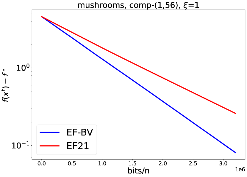
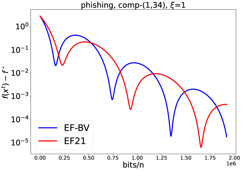
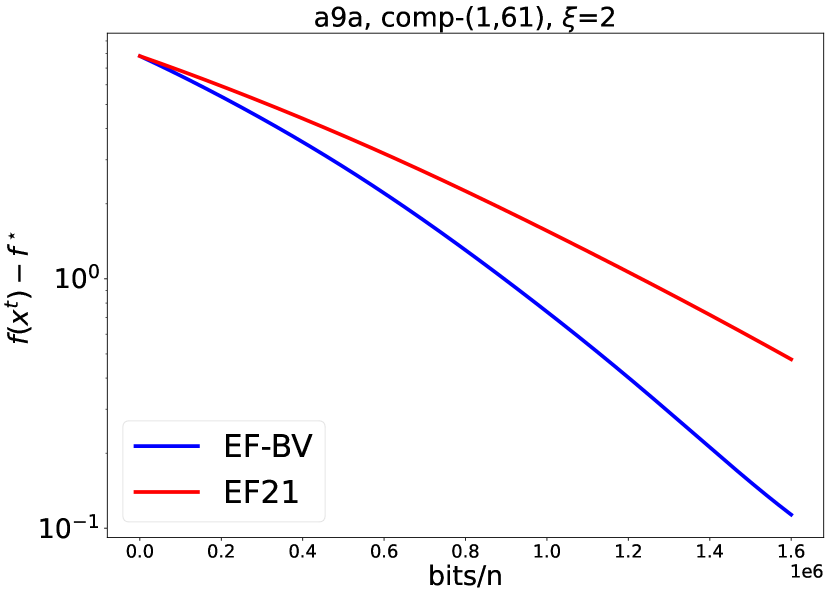
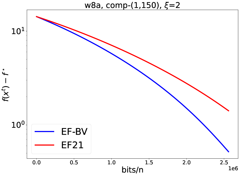
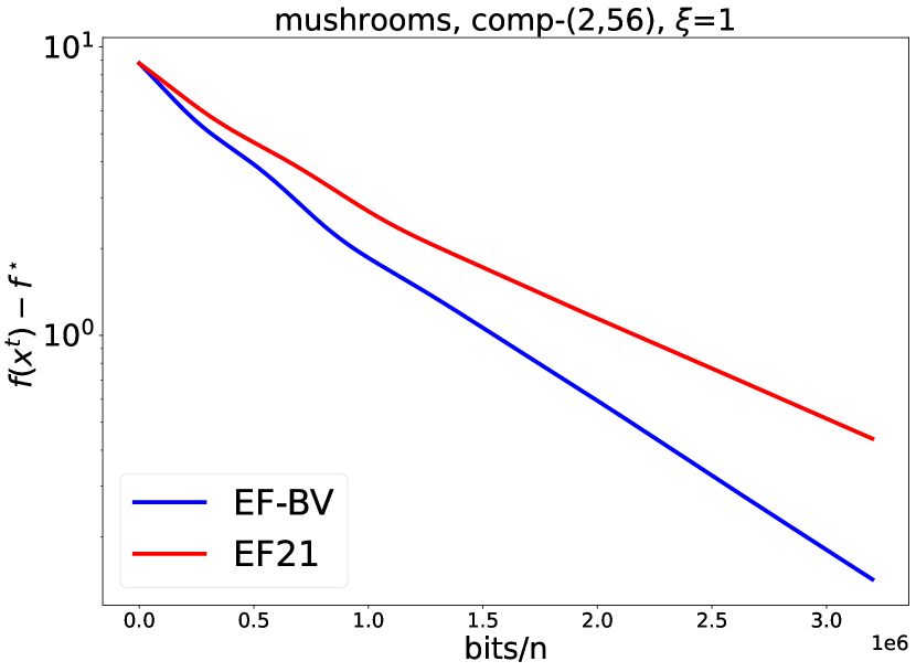
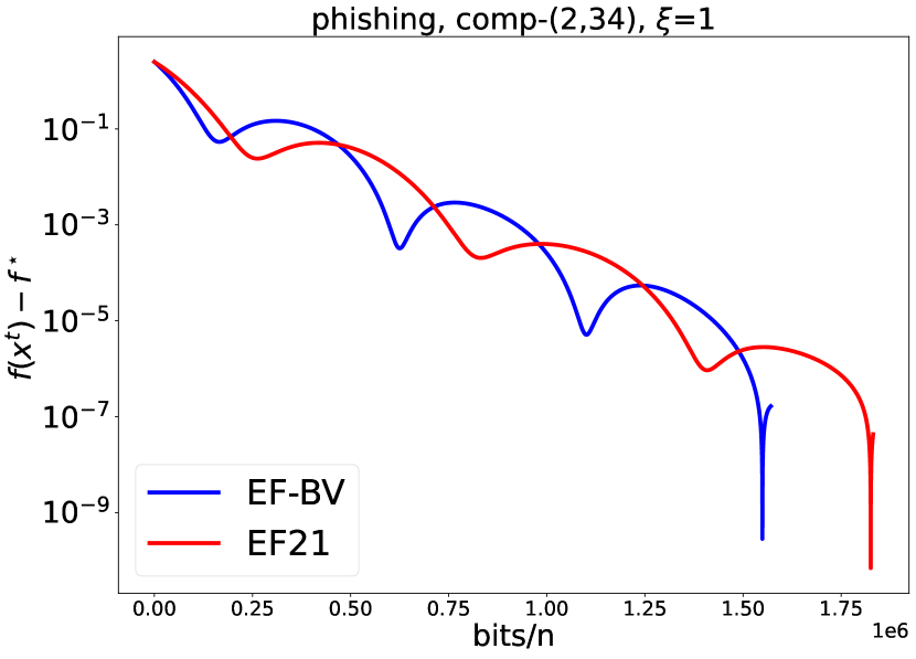
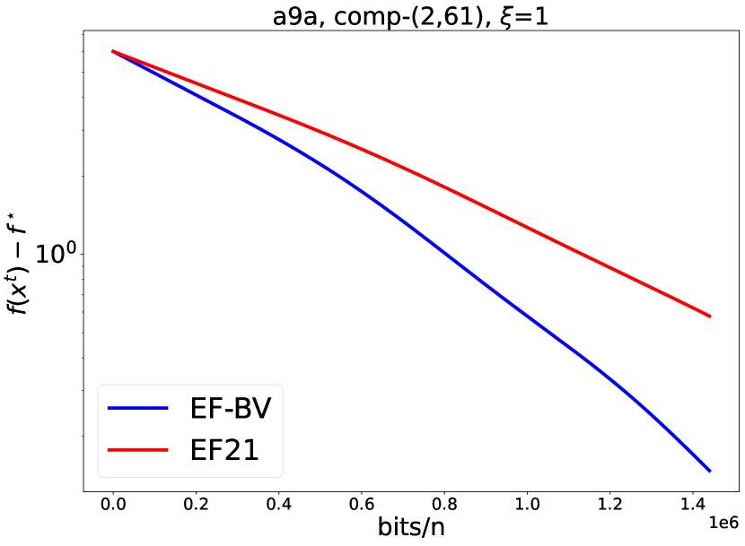
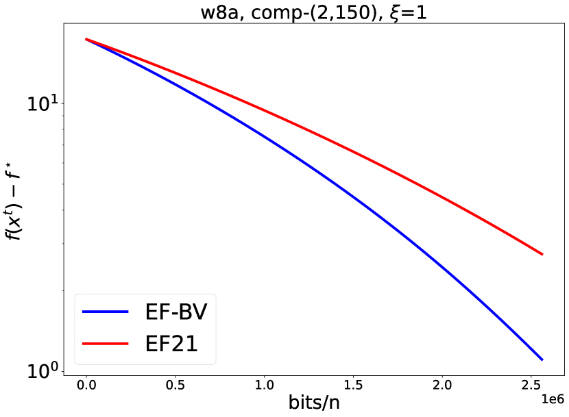
Figure 2: Experimental results. We plot $f(x^{t})-f^{\star}$ with respect to the number of bits sent by each node during the learning process, which is proportional to $tk$. Top row: comp-$(1,d/2)$, overlapping $\xi=1$. Middle row: comp-$(1,d/2)$, overlapping $\xi=2$. Bottom row: comp-$(2,d/2)$, overlapping $\xi=1$.

Appendix

Contents

1. 1 Introduction
2. 2 Compressors and their properties
   1. 2.1 Unbiased compressors
   2. 2.2 Biased contractive compressors
   3. 2.3 New general class of compressors
   4. 2.4 Average variance of several compressors
   5. 2.5 Scaling compressors
3. 3 Proposed algorithm EF-BV
   1. 3.1 EF21 as a particular case of EF-BV
   2. 3.2 DIANA as a particular case of EF-BV
4. 4 Linear convergence results
   1. 4.1 Implications for EF21
   2. 4.2 Implications for DIANA
5. 5 Sublinear convergence in the nonconvex case
6. 6 Experiments
7. A New compressors
   1. A.1 mix-(k,k’): Mixture of top-k and rand-k
   2. A.2 comp-(k,k’): Composition of top-k and rand-k
8. B New results on DIANA
9. C Experiments
   1. C.1 Datasets and experimental setup
   2. C.2 Experimental results and analysis
   3. C.3 Additional experiments in the nonconvex setting
10. D Proof of Proposition 4
11. E Proof of Proposition 5
12. F Proof of Theorem 1
13. G Proof of Theorem 2
14. H Proof of Theorem 3

Appendix A New compressors

We propose new compressors in our class $\mathbb{C}(\eta,\omega)$.

A.1 mix-(k,k’): Mixture of top-k and rand-k

Let $k\in\mathcal{I}_{d}$ and $k^{\prime}\in\mathcal{I}_{d}$, with $k+k^{\prime}\leq d$. We propose the compressor mix-$(k,k^{\prime})$. It maps $x\in\mathbb{R}^{d}$ to $x^{\prime}\in\mathbb{R}^{d}$, defined as follows. Let $i_{1},\ldots,i_{k}$ be distinct indexes in $\mathcal{I}_{d}$ such that $|x_{i_{1}}|,\ldots,|x_{i_{k}}|$ are the $k$ largest elements of $|x|$ (if this selection is not unique, we can choose any one). These coordinates are kept: $x^{\prime}_{i_{j}}=x_{i_{j}}$, $j=1,\ldots,k$. In addition, $k^{\prime}$ other coordinates chosen at random in the remaining ones are kept: $x^{\prime}_{i_{j}}=x_{i_{j}}$, $j=k+1,\ldots,k+k^{\prime}$, where $\{i_{j}:j=k+1,\ldots,k+k^{\prime}\}$ is a subset of size $k^{\prime}$ of $\mathcal{I}_{d}\backslash\{i_{1},\ldots,i_{k}\}$ chosen uniformly at random. The other coordinates of $x^{\prime}$ are set to zero.

Proposition 4.

mix-$(k,k^{\prime})\in\mathbb{C}(\eta,\omega)$ with $\eta=\frac{d-k-k^{\prime}}{\sqrt{(d-k)d}}$ and $\omega=\frac{k^{\prime}(d-k-k^{\prime})}{(d-k)d}$.

As a consequence, mix-$(k,k^{\prime})\in\mathbb{B}(\alpha)$ with $\alpha=1-\eta^{2}-\omega=1-\frac{(d-k-k^{\prime})^{2}}{(d-k)d}-\frac{k^{\prime}(d-k-k^{\prime})}{(d-k)d}=\frac{k+k^{\prime}}{d}$. This is the same $\alpha$ as for top-$(k+k^{\prime})$ and scaled rand-$(k+k^{\prime})$.

The proof is given in Appendix D.

A.2 comp-(k,k’): Composition of top-k and rand-k

Let $k\in\mathcal{I}_{d}$ and $k^{\prime}\in\mathcal{I}_{d}$, with $k\leq k^{\prime}$. We consider the compressor comp-$(k,k^{\prime})$, proposed in Barnes et al. (2020), which is the composition of top-$k^{\prime}$ and rand-$k$: top-$k^{\prime}$ is applied first, then rand-$k$ is applied to the $k^{\prime}$ selected (largest) elements. That is, comp-$(k,k^{\prime})$ maps $x\in\mathbb{R}^{d}$ to $x^{\prime}\in\mathbb{R}^{d}$, defined as follows. Let $i_{1},\ldots,i_{k^{\prime}}$ be distinct indexes in $\mathcal{I}_{d}$ such that $|x_{i_{1}}|,\ldots,|x_{i_{k^{\prime}}}|$ are the $k^{\prime}$ largest elements of $|x|$ (if this selection is not unique, we can choose any one). Then $x^{\prime}_{i_{j}}=\frac{k^{\prime}}{k}x_{i_{j}}$, $j=1,\ldots,k$, where $\{i_{j}:j=1,\ldots,k\}$ is a subset of size $k$ of $\{i_{1},\ldots,i_{k^{\prime}}\}$ chosen uniformly at random. The other coordinates of $x^{\prime}$ are set to zero.

comp-$(k,k^{\prime})$ sends $k$ coordinates of its input vector, like top-$k$ and rand-$k$, whatever $k^{\prime}$. We can note that comp-$(k,d)={}$rand-$k$ and comp-$(k,k)={}$top-$k$. We have:

Proposition 5.

comp-$(k,k^{\prime})\in\mathbb{C}(\eta,\omega)$ with $\eta=\sqrt{\frac{d-k^{\prime}}{d}}$ and $\omega=\frac{k^{\prime}-k}{k}$.

The proof is given in Appendix E.

Appendix B New results on DIANA

We suppose that the compressors $\mathcal{C}_{i}^{t}$ are in $\mathbb{C}(\eta,\omega)$, for some $\eta\in[0,1)$ and $\omega\geq 0$. Viewing DIANA as EF-BV with $\nu=1$, we define $r$, $s^{\star}$, $\theta^{\star}$ as before, as well as $r_{\mathrm{av}}\coloneqq\eta^{2}+\omega_{\mathrm{av}}$. We obtain, as corollaries of Theorems 1 and 2:

Theorem 4.

Suppose that $R=0$ and $f$ satisfies the PŁ condition with some constant $\mu>0$. In DIANA, suppose that $\lambda\in(0,1]$ is such that $r<1$, and

$$0<\gamma\leq\frac{1}{L+\tilde{L}\sqrt{\frac{r_{\mathrm{av}}}{r}}\frac{1}{s^{\star}}}.$$

For every $t\geq 0$, define the Lyapunov function $\Psi^{t}\coloneqq f(x^{t})-f^{\star}+\frac{\gamma}{2\theta^{\star}}\frac{1}{n}\sum_{i=1}^{n}\left\|\nabla f_{i}(x^{t})-h_{i}^{t}\right\|^{2}$, where $f^{\star}\coloneqq f(x^{\star})$, for any minimizer $x^{\star}$ of $f$. Then, for every $t\geq 0$,

$$\mathbb{E}\!\left[\Psi^{t}\right] \leq\left(\max\left(1-\gamma\mu,{\frac{r+1}{2}}\right)\right)^{t}\Psi^{0}.$$

Theorem 5.

Suppose that $f+R$ satisfies the the KŁ condition with some constant $\mu>0$. In DIANA, suppose that $\lambda\in(0,1]$ is such that $r<1$, and

$$0<\gamma\leq\frac{1}{2L+\tilde{L}\sqrt{\frac{r_{\mathrm{av}}}{r}}\frac{1}{s^{\star}}}.$$

$\forall t\geq 0$, define the Lyapunov function $\Psi^{t}\coloneqq f(x^{t})+R(x^{t})-f^{\star}-R^{\star}+\frac{\gamma}{2\theta^{\star}}\frac{1}{n}\sum_{i=1}^{n}\left\|\nabla f_{i}(x^{t})-h_{i}^{t}\right\|^{2}$, where $f^{\star}\coloneqq f(x^{\star})$ and $R^{\star}\coloneqq R(x^{\star})$, for any minimizer $x^{\star}$ of $f+R$. Then, for every $t\geq 0$,

$$\mathbb{E}\!\left[\Psi^{t}\right] \leq\left(\max\left({\frac{1}{1+\frac{1}{2}\gamma\mu}},\frac{r+1}{2}\right)\right)^{t}\Psi^{0}.$$

Interestingly, DIANA, used beyond its initial setting with compressors in $\mathbb{B}(\alpha)$ with $\lambda=1$, just reverts to (the original) EF21, as shown in Fig. 1. This shows how our unified framework reveals connections between these two algorithms and unleashes their potential.

Appendix C Experiments

C.1 Datasets and experimental setup

We consider the heterogeneous data distributed regime, which means that all parallel nodes store different data points, but use the same type of learning function. We adopt the datasets from LibSVM (Chang & Lin, 2011) and we split them, after random shuffling, into $n\leq N$ blocks, where $N$ is the total number of data points (the left-out data points from the integer division of $N$ by $n$ are stored at the last node). The corresponding values are shown in Tab. 2. To make our setting more realistic, we consider that different nodes partially share some data: we set the overlapping factor to be $\xi\in\{1,2\}$, where $\xi=1$ means no overlap and $\xi=2$ means that the data is partially shared among the nodes, with a redundancy factor of 2; this is achieved by sequentially assigning 2 blocks of data to every node. The experiments were conducted using 24 NVIDIA-A100-80G GPUs, each with 80GB memory.

Table 2: Values of $d$ and $N$ for the considered datasets.

Dataset	$N$ (total # of datapoints)	$d$ (# of features)
mushrooms	8,124	112
phishing	11,055	68
a9a	32,561	123
w8a	49,749	300

We consider logistic regression, which consists in minimizing the $\mu$-strongly convex function

$$f=\frac{1}{n}\sum_{i=1}^{n}f_{i},$$

with, for every $i\in\mathcal{I}_{n}$,

$$f_{i}(x)=\frac{1}{N_{i}}\sum_{j=1}^{N_{i}}\log\!\Big{(}1+\exp\!\left(-b_{i,j}x^{\top}a_{i,j}\right)\Big{)}+\frac{\mu}{2}\|x\|^{2},$$

where $\mu$, set to $0.1$, is the strong convexity constant; $N_{i}$ is the number of data points at node $i$; the $a_{i,j}$ are the training vectors and the $b_{i,j}\in\{-1,1\}$ the corresponding labels. Note that there is no regularizer in this problem; that is, $R=0$.

We set $L=\tilde{L}=\sqrt{\sum_{i=1}^{n}L_{i}^{2}}$, with $L_{i}=\mu+\frac{1}{4N_{i}}\sum_{j=1}^{N_{i}}\|a_{i,j}\|^{2}$. We use independent compressors of type comp-$(k,k^{\prime})$ at every node, for some small $k$ and large $k^{\prime}<d$. These compressors are biased ($\eta>0$) and have a variance $\omega>1$, so they are not contractive: they don’t belong to $\mathbb{B}(\alpha)$ for any $\alpha$. We have $\omega_{\mathrm{av}}=\frac{\omega}{n}$. Thus, we place ourselves in the conditions of Theorem 1, and we compare EF-BV with

$$\lambda=\lambda^{\star},\quad\nu=\nu^{\star},\quad\gamma=\frac{1}{L+\tilde{L}\sqrt{\frac{r_{\mathrm{av}}}{r}}\frac{1}{s^{\star}}}$$

to EF21, which corresponds to the particular case of EF-BV with

$$\nu=\lambda=\lambda^{\star},\quad\gamma=\frac{1}{L+\tilde{L}\frac{1}{s^{\star}}}.$$

Table 3: Parameter values of EF-BV and EF21 in the different settings. $k^{\prime}$ in comp-$(k,k^{\prime})$ is set to $d/2$ and $n=1000$. In pairs of values like (1,2), the first value is $k$ and the second value is $\xi$.

Method	Params	mushrooms			phishing			a9a			w8a
		(1,1)	(1,2)	(2,1)	(1,1)	(1,2)	(2,1)	(1,1)	(1,2)	(2,1)	(1,1)	(1,2)	(2,1)
	$\eta$	0.707	0.707	0.707	0.707	0.707	0.707	0.710	0.710	0.710	0.707	0.707	0.707
	$\omega$	55	55	27	33	33	16	60	60	29.5	149	149	74
	$\omega_{\mathrm{av}}$	0.055	0.055	0.027	0.033	0.033	0.016	0.06	0.06	0.295	0.149	0.149	0.074
EF-BV	$\lambda$	5.32e-3	5.32e-3	1.08e-2	8.85e-3	8.85e-3	1.82e-2	4.83e-3	4.83e-3	9.8e-3	1.96e-3	1.96e-3	3.95e-3
EF21		5.32e-3	5.32e-4	1.08e-2	8.85e-3	8.85e-3	1.82e-2	4.83e-3	4.83e-3	9.8e-3	1.96e-3	1.96e-3	3.95e-3
EF-BV	$\nu$	1	1	1	1	1	1	1	1	1	1	1	1
EF21		5.32e-3	5.32e-4	1.08e-2	8.85e-3	8.85e-3	1.82e-2	4.83e-3	4.83e-3	9.8e-3	1.96e-3	1.96e-3	3.95e-3
EF-BV	$r$	0.998	0.998	0.997	0.997	0.997	0.994	0.999	0.999	0.997	0.999	0.999	0.999
EF21		0.998	0.998	0.997	0.997	0.997	0.994	0.999	0.999	0.997	0.999	0.999	0.999
EF-BV	$r_{\mathrm{av}}$	0.555	0.555	0.527	0.533	0.533	0.516	0.564	0.564	0.534	0.649	0.649	0.574
EF21		0.998	0.998	0.997	0.997	0.997	0.994	0.999	0.999	0.997	0.999	0.999	0.999
EF-BV	$\sqrt{\frac{r_{\mathrm{av}}}{r}}$	0.746	0.746	0.727	0.731	0.731	0.720	0.752	0.752	0.731	0.806	0.806	0.758
EF21		1	1	1	1	1	1	1	1	1	1	1	1
EF-BV	$s^{\star}$	3.90e-4	3.90e-4	7.94e-4	6.50e-4	6.50e-4	1.34e-3	3.5e-4	3.5e-4	7.13e-4	1.44e-4	1.44e-4	2.90e-4
EF21		3.90e-4	3.90e-4	7.94e-4	6.50e-4	6.50e-4	1.34e-3	3.5e-4	3.5e-4	7.13e-4	1.44e-4	1.44e-4	2.90e-4
EF-BV	$\gamma$	1.38e-4	1.43e-4	2.87e-4	2.33e-3	2.36e-3	4.80e-3	2.53e-4	2.58e-4	5.28e-4	1.01e-4	1.15e-4	2.15e-4
EF21		1.03e-4	1.06e-4	2.10e-4	1.71e-3	1.73e-3	3.49e-3	1.91e-4	1.84e-4	3.87e-4	8.12e-5	9.31e-5	1.63e-4

C.2 Experimental results and analysis

We show in Fig. 2 the results with $k=1$ or $k=2$ in the compressors comp-$(k,k^{\prime})$, and overlapping factor $\xi=1$ or $\xi=2$. We chose $k^{\prime}=\frac{d}{2}$ and $n=1000$. The corresponding values of $\eta$, $\omega$, $\omega_{\mathrm{av}}$, and the parameter values used in the algorithms are shown in Tab. 3. We can see that there is essentially no difference between the two choices $\xi=1$ and $\xi=2$, and the qualitative behavior for $k=1$ and $k=2$ is similar. Thus, we observe that EF-BV converges always faster than EF21; this is consistent with our analysis.

We tried other values of $n$, including the largest value $n=N$, for which there is only one data point at every node. The behavior of EF21 and EF-BV was the same as for $n=1000$, so we don’t show the results.

We tried other values of $k^{\prime}$. The behavior of EF21 and EF-BV was the same as for $k^{\prime}=\frac{d}{2}$ overall, so we don’t show the results. We noticed that the difference between the two algorithms was smaller when $k^{\prime}$ was smaller; this is expected, since for $k^{\prime}=k$, the compressors revert to top-$k$, for which EF21 and EF-BV are the same algorithm.

To sum up, the experiments confirm our analysis: when $\omega$ and $n$ are large, so that the key factor $\sqrt{\frac{r_{\mathrm{av}}}{r}}$ is small, randomness is exploited in EF-BV, with larger values of $\nu$ and $\gamma$ allowed than in EF21, and this yields faster convergence.

In future work, we will design and compare other compressors in our new class $\mathbb{C}(\eta,\omega)$, performing well in both homogeneous and heterogeneous regimes.

C.3 Additional experiments in the nonconvex setting

We consider the logistic regression problem with a nonconvex regularizer:

$$f(x)=\frac{1}{n}\sum_{i=1}^{n}\log\left(1+\exp\left(-y_{i}a_{i}^{\top}x\right)\right)+\lambda\sum_{j=1}^{d}\frac{x_{j}^{2}}{1+x_{j}^{2}},$$ (15)

where $a_{i}\in\mathbb{R}^{d},y_{i}\in\{-1,1\}$ are the training data, and $\lambda>0$ is the regularizer parameter. We used $\lambda=0.1$ in all experiments. We present the results in Fig. 3.

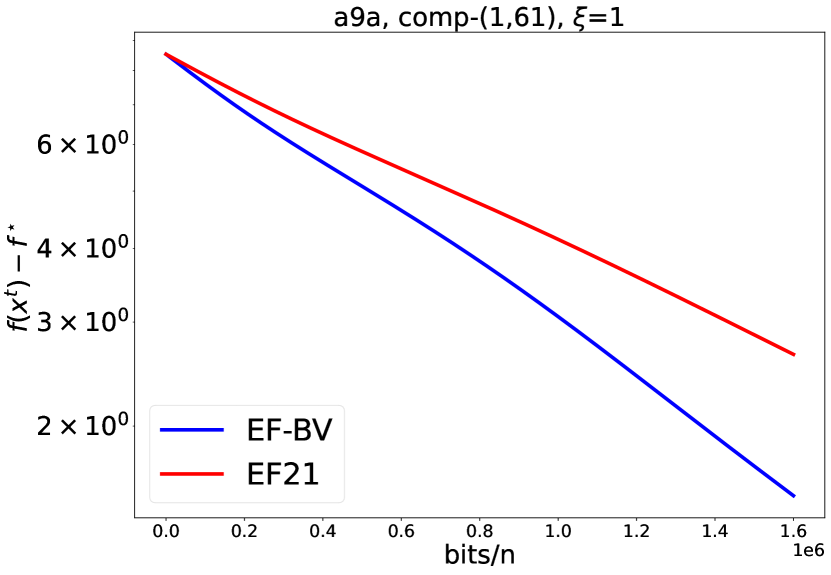
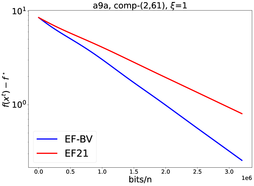
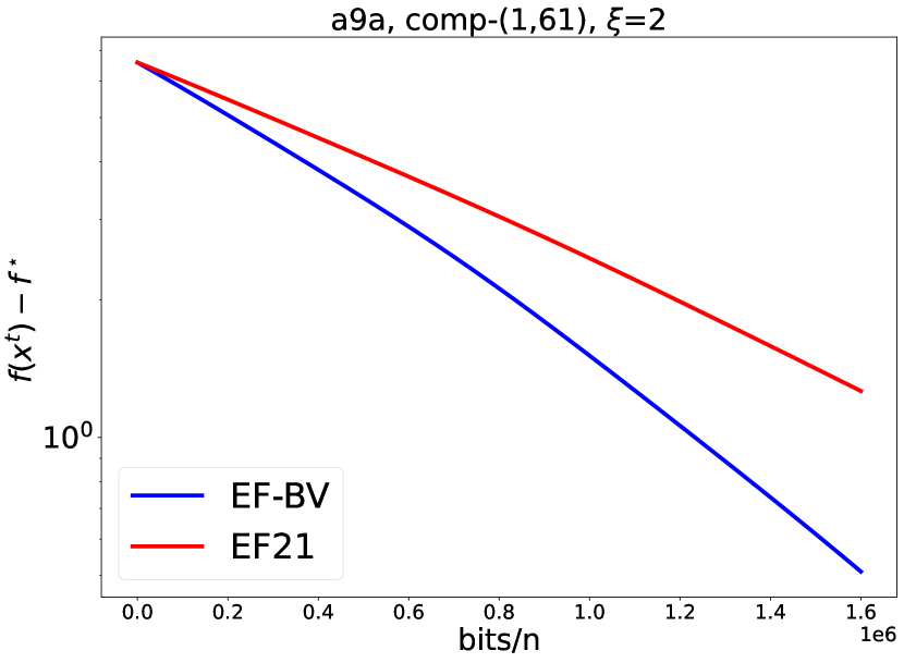
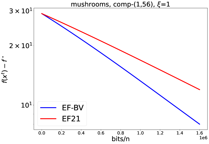
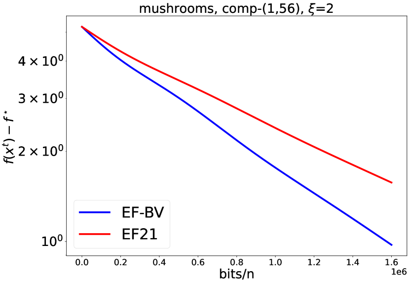
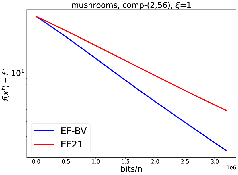
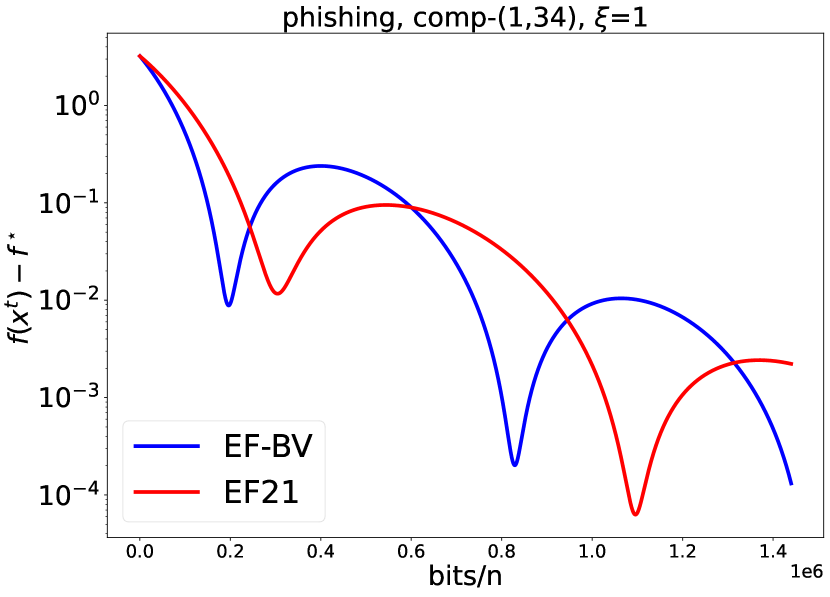
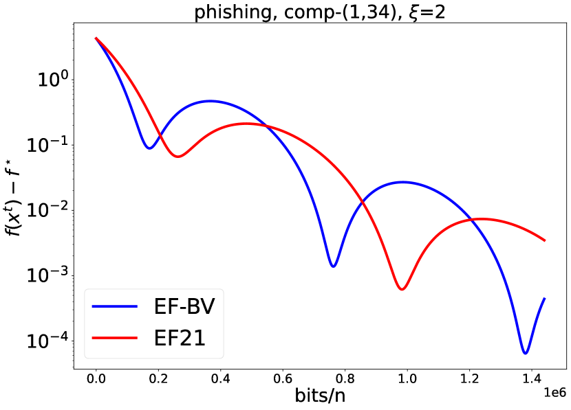
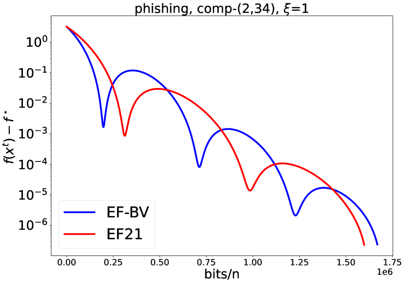
Figure 3: Comparison between EF21 and EF-BV in the nonconvex setting. We see that EF-BV outperforms EF21 for all datasets.

Appendix D Proof of Proposition 4

We first calculate $\omega$. Let $x\in\mathbb{R}^{d}$.

$$\big{\|}\mathcal{C}(x)-\mathbb{E}[\mathcal{C}(x)]\big{\|}^{2} =\sum_{i\in\mathcal{I}_{d}\backslash\{i_{1},\ldots,i_{k+k^{\prime}}\}}\left(\frac{k^{\prime}}{d-k}\right)^{2}|x_{i}|^{2}+\sum_{j=k+1}^{k+k^{\prime}}\left(\frac{d-k-k^{\prime}}{d-k}\right)^{2}|x_{i_{j}}|^{2}.$$

Therefore, by taking the expectation over the random indexes $i_{k+1},\ldots,i_{2k}$,

$$\mathbb{E}\!\left[\big{\|}\mathcal{C}(x)-\mathbb{E}[\mathcal{C}(x)]\big{\|}^{2}\right] =\sum_{i\in\mathcal{I}_{d}\backslash\{i_{1},\ldots,i_{k}\}}\left(\frac{d-k-k^{\prime}}{d-k}\left(\frac{k^{\prime}}{d-k}\right)^{2}+\frac{k^{\prime}}{d-k}\left(\frac{d-k-k^{\prime}}{d-k}\right)^{2}\right)|x_{i}|^{2}$$

$$=\frac{k^{\prime}(d-k-k^{\prime})}{(d-k)^{2}}\sum_{i\in\mathcal{I}_{d}\backslash\{i_{1},\ldots,i_{k}\}}|x_{i}|^{2}.$$

Moreover, since the $|x_{i_{j}}|$ are the largest elements of $|x|$, for every $j=1,\ldots,k$,

$$|x_{i_{j}}|^{2}\geq\frac{1}{d-k}\sum_{i\in\mathcal{I}_{d}\backslash\{i_{1},\ldots,i_{k}\}}|x_{i}|^{2},$$

so that

$$\|x\|^{2}=\sum_{i\in\mathcal{I}_{d}}|x_{i}|^{2}\geq\left(1+\frac{k}{d-k}\right)\sum_{i\in\mathcal{I}_{d}\backslash\{i_{1},\ldots,i_{k}\}}|x_{i}|^{2}.$$

Hence,

$$\mathbb{E}\!\left[\big{\|}\mathcal{C}(x)-\mathbb{E}[\mathcal{C}(x)]\big{\|}^{2}\right] \leq\frac{k^{\prime}(d-k-k^{\prime})}{(d-k)^{2}}\frac{d-k}{d}\|x\|^{2}=\frac{k^{\prime}(d-k-k^{\prime})}{(d-k)d}\|x\|^{2}.$$

Then, let us calculate $\eta$.

$$\big{\|}\mathbb{E}[\mathcal{C}(x)]-x\big{\|}^{2} =\sum_{i\in\mathcal{I}_{d}\backslash\{i_{1},\ldots,i_{k}\}}\left(\frac{d-k-k^{\prime}}{d-k}\right)^{2}|x_{i}|^{2}$$

$$\leq\frac{(d-k-k^{\prime})^{2}}{(d-k)d}\|x\|^{2}.$$

Thus, $\eta=\frac{d-k-k^{\prime}}{\sqrt{(d-k)d}}$.

Appendix E Proof of Proposition 5

We first calculate $\omega$. Let $x\in\mathbb{R}^{d}$.

$$\big{\|}\mathcal{C}(x)-\mathbb{E}[\mathcal{C}(x)]\big{\|}^{2} =\sum_{j\in\{j_{1},\ldots,j_{k}\}}\left(\frac{k^{\prime}-k}{k}\right)^{2}|x_{i_{j}}|^{2}+\sum_{i\in\{i_{1},\ldots,i_{k^{\prime}}\}\backslash\{i_{j_{1}},\ldots,i_{j_{k}}\}}|x_{i}|^{2}$$

Therefore, by taking the expectation over the random indexes $i_{j_{1}},\ldots,i_{j_{k}}$,

$$\mathbb{E}\!\left[\big{\|}\mathcal{C}(x)-\mathbb{E}[\mathcal{C}(x)]\big{\|}^{2}\right] =\sum_{j=1}^{k^{\prime}}\left(\frac{k}{k^{\prime}}\left(\frac{k^{\prime}-k}{k}\right)^{2}+\frac{k^{\prime}-k}{k^{\prime}}\right)|x_{i_{j}}|^{2}$$

$$=\frac{k^{\prime}-k}{k}\sum_{j=1}^{k^{\prime}}|x_{i_{j}}|^{2}$$

$$\leq\frac{k^{\prime}-k}{k}\|x\|^{2}$$

Then, let us calculate $\eta$:

$$\big{\|}\mathbb{E}[\mathcal{C}(x)]-x\big{\|}^{2}=\sum_{i\in\mathcal{I}_{d}\backslash\{i_{1},\ldots,i_{k^{\prime}}\}}|x_{i}|^{2}\leq\frac{d-k^{\prime}}{d}\|x\|^{2}.$$

Appendix F Proof of Theorem 1

We have the descent property (Richtárik et al., 2021, Lemma 4), for every $t\geq 0$,

$$f(x^{t+1})-f^{\star} \leq f(x^{t})-f^{\star}-\frac{\gamma}{2}\left\|\nabla f(x^{t})\right\|^{2}+\frac{\gamma}{2}\left\|g^{t+1}-\nabla f(x^{t})\right\|^{2}$$

$$\quad+\left(\frac{L}{2}-\frac{1}{2\gamma}\right)\left\|x^{t+1}-x^{t}\right\|^{2}$$ (16)

$$\leq(1-\gamma\mu)\big{(}f(x^{t})-f^{\star}\big{)}+\frac{\gamma}{2}\left\|g^{t+1}-\nabla f(x^{t})\right\|^{2}+\left(\frac{L}{2}-\frac{1}{2\gamma}\right)\left\|x^{t+1}-x^{t}\right\|^{2}.$$

Then, for every $t\geq 0$, conditionally on $x^{t}$, $h^{t}$ and $(h_{i}^{t})_{i=1}^{n}$,

$$\mathbb{E}\!\left[\left\|g^{t+1}-\nabla f(x^{t})\right\|^{2}\right] =\mathbb{E}\!\left[\left\|\frac{1}{n}\sum_{i=1}^{n}\Big{(}h_{i}^{t}-\nabla f_{i}(x^{t})+\nu\mathcal{C}_{i}^{t}\big{(}\nabla f_{i}(x^{t})-h_{i}^{t}\big{)}\Big{)}\right\|^{2}\right]$$

$$=\left\|\frac{1}{n}\sum_{i=1}^{n}\Big{(}h_{i}^{t}-\nabla f_{i}(x^{t})+\nu\mathbb{E}\!\left[\mathcal{C}_{i}^{t}\big{(}\nabla f_{i}(x^{t})-h_{i}^{t}\big{)}\right]\Big{)}\right\|^{2}$$

$$\quad+\nu^{2}\mathbb{E}\!\left[\left\|\frac{1}{n}\sum_{i=1}^{n}\Big{(}\mathcal{C}_{i}^{t}\big{(}\nabla f_{i}(x^{t})-h_{i}^{t}\big{)}-\mathbb{E}\!\left[\mathcal{C}_{i}^{t}\big{(}\nabla f_{i}(x^{t})-h_{i}^{t}\big{)}\right]\Big{)}\right\|^{2}\right]$$

$$\leq\left\|\frac{1}{n}\sum_{i=1}^{n}\Big{(}h_{i}^{t}-\nabla f_{i}(x^{t})+\nu\mathbb{E}\!\left[\mathcal{C}_{i}^{t}\big{(}\nabla f_{i}(x^{t})-h_{i}^{t}\big{)}\right]\Big{)}\right\|^{2}$$

$$\quad+\nu^{2}\frac{\omega_{\mathrm{av}}}{n}\sum_{i=1}^{n}\left\|\nabla f_{i}(x^{t})-h_{i}^{t}\right\|^{2},$$

where the last inequality follows from (6). In addition,

$$\left\|\frac{1}{n}\sum_{i=1}^{n}\Big{(}h_{i}^{t}-\nabla f_{i}(x^{t})+\nu\mathbb{E}\!\left[\mathcal{C}_{i}^{t}\big{(}\nabla f_{i}(x^{t})-h_{i}^{t}\big{)}\right]\Big{)}\right\|$$

$$\quad\leq\left\|\frac{1}{n}\sum_{i=1}^{n}\Big{(}\nu\big{(}h_{i}^{t}-\nabla f_{i}(x^{t})\big{)}+\nu\mathbb{E}\!\left[\mathcal{C}_{i}^{t}\big{(}\nabla f_{i}(x^{t})-h_{i}^{t}\big{)}\right]\Big{)}\right\|$$

$$\quad\quad+(1-\nu)\left\|\frac{1}{n}\sum_{i=1}^{n}\big{(}h_{i}^{t}-\nabla f_{i}(x^{t})\big{)}\right\|$$

$$\quad\leq\frac{\nu}{n}\sum_{i=1}^{n}\left\|h_{i}^{t}-\nabla f_{i}(x^{t})+\mathbb{E}\!\left[\mathcal{C}_{i}^{t}\big{(}\nabla f_{i}(x^{t})-h_{i}^{t}\big{)}\right]\right\|$$

$$\quad\quad+\frac{1-\nu}{n}\sum_{i=1}^{n}\left\|h_{i}^{t}-\nabla f_{i}(x^{t})\right\|$$

$$\quad\leq\frac{\nu\eta}{n}\sum_{i=1}^{n}\left\|\nabla f_{i}(x^{t})-h_{i}^{t}\right\|+\frac{1-\nu}{n}\sum_{i=1}^{n}\left\|\nabla f_{i}(x^{t})-h_{i}^{t}\right\|$$

$$\quad=\frac{1-\nu+\nu\eta}{n}\sum_{i=1}^{n}\left\|\nabla f_{i}(x^{t})-h_{i}^{t}\right\|.$$

Therefore,

$$\left\|\frac{1}{n}\sum_{i=1}^{n}\Big{(}h_{i}^{t}-\nabla f_{i}(x^{t})+\nu\mathbb{E}\!\left[\mathcal{C}_{i}^{t}\big{(}\nabla f_{i}(x^{t})-h_{i}^{t}\big{)}\right]\Big{)}\right\|^{2}\leq\frac{(1-\nu+\nu\eta)^{2}}{n}\sum_{i=1}^{n}\left\|\nabla f_{i}(x^{t})-h_{i}^{t}\right\|^{2},$$

and, conditionally on $x^{t}$, $h^{t}$ and $(h_{i}^{t})_{i=1}^{n}$,

$$\mathbb{E}\!\left[\left\|g^{t+1}-\nabla f(x^{t})\right\|^{2}\right] \leq\left((1-\nu+\nu\eta)^{2}+\nu^{2}\omega_{\mathrm{av}}\right)\frac{1}{n}\sum_{i=1}^{n}\left\|\nabla f_{i}(x^{t})-h_{i}^{t}\right\|^{2}.$$

Thus, for every $t\geq 0$, conditionally on $x^{t}$, $h^{t}$ and $(h_{i}^{t})_{i=1}^{n}$,

$$\mathbb{E}\!\left[f(x^{t+1})-f^{\star}\right] \leq(1-\gamma\mu)\big{(}f(x^{t})-f^{\star}\big{)}+\frac{\gamma}{2}\big{(}(1-\nu+\nu\eta)^{2}+\nu^{2}\omega_{\mathrm{av}}\big{)}\frac{1}{n}\sum_{i=1}^{n}\left\|\nabla f_{i}(x^{t})-h_{i}^{t}\right\|^{2}$$

$$\quad+\left(\frac{L}{2}-\frac{1}{2\gamma}\right)\mathbb{E}\!\left[\left\|x^{t+1}-x^{t}\right\|^{2}\right].$$

Now, let us study the control variates $h_{i}^{t}$. Let $s>0$. Using the Peter–Paul inequality $\|a+b\|^{2}\leq(1+s)\|a\|^{2}+(1+s^{-1})\|b\|^{2}$, for any vectors $a$ and $b$, we have, for every $t\geq 0$ and $i\in\mathcal{I}_{n}$,

$$\left\|\nabla f_{i}(x^{t+1})-h_{i}^{t+1}\right\|^{2} =\left\|h_{i}^{t}-\nabla f_{i}(x^{t+1})+\lambda\mathcal{C}_{i}^{t}\big{(}\nabla f_{i}(x^{t})-h_{i}^{t}\big{)}\right\|^{2}$$

$$\leq(1+s)\left\|h_{i}^{t}-\nabla f_{i}(x^{t})+\lambda\mathcal{C}_{i}^{t}\big{(}\nabla f_{i}(x^{t})-h_{i}^{t}\big{)}\right\|^{2}$$

$$\quad+(1+s^{-1})\left\|\nabla f_{i}(x^{t+1})-\nabla f_{i}(x^{t})\right\|^{2}$$

$$\leq(1+s)\left\|h_{i}^{t}-\nabla f_{i}(x^{t})+\lambda\mathcal{C}_{i}^{t}\big{(}\nabla f_{i}(x^{t})-h_{i}^{t}\big{)}\right\|^{2}$$

$$\quad+(1+s^{-1})L_{i}^{2}\left\|x^{t+1}-x^{t}\right\|^{2}.$$

Moreover, conditionally on $x^{t}$, $h^{t}$ and $(h_{i}^{t})_{i=1}^{n}$,

$$\mathbb{E}\!\left[\left\|h_{i}^{t}-\nabla f_{i}(x^{t})+\lambda\mathcal{C}_{i}^{t}\big{(}\nabla f_{i}(x^{t})-h_{i}^{t}\big{)}\right\|^{2}\right] =\left\|h_{i}^{t}-\nabla f_{i}(x^{t})+\lambda\mathbb{E}\!\left[\mathcal{C}_{i}^{t}\big{(}\nabla f_{i}(x^{t})-h_{i}^{t}\big{)}\right]\right\|^{2}$$

$$\quad+\lambda^{2}\mathbb{E}\!\left[\left\|\mathcal{C}_{i}^{t}\big{(}\nabla f_{i}(x^{t})-h_{i}^{t}\big{)}-\mathbb{E}\!\left[\mathcal{C}_{i}^{t}\big{(}\nabla f_{i}(x^{t})-h_{i}^{t}\big{)}\right]\right\|^{2}\right]$$

$$\leq\left\|h_{i}^{t}-\nabla f_{i}(x^{t})+\lambda\mathbb{E}\!\left[\mathcal{C}_{i}^{t}\big{(}\nabla f_{i}(x^{t})-h_{i}^{t}\big{)}\right]\right\|^{2}$$

$$\quad+\lambda^{2}\omega\left\|\nabla f_{i}(x^{t})-h_{i}^{t}\right\|^{2}.$$

In addition,

$$\left\|h_{i}^{t}-\nabla f_{i}(x^{t})+\lambda\mathbb{E}\!\left[\mathcal{C}_{i}^{t}\big{(}\nabla f_{i}(x^{t})-h_{i}^{t}\big{)}\right]\right\| \leq\left\|\lambda\big{(}h_{i}^{t}-\nabla f_{i}(x^{t})\big{)}+\lambda\mathbb{E}\!\left[\mathcal{C}_{i}^{t}\big{(}\nabla f_{i}(x^{t})-h_{i}^{t}\big{)}\right]\right\|$$

$$\quad+(1-\lambda)\left\|h_{i}^{t}-\nabla f_{i}(x^{t})\right\|$$

$$\leq\lambda\eta\left\|\nabla f_{i}(x^{t})-h_{i}^{t}\right\|+(1-\lambda)\left\|\nabla f_{i}(x^{t})-h_{i}^{t}\right\|$$

$$=(1-\lambda+\lambda\eta)\left\|\nabla f_{i}(x^{t})-h_{i}^{t}\right\|.$$

Therefore, conditionally on $x^{t}$, $h^{t}$ and $(h_{i}^{t})_{i=1}^{n}$,

$$\mathbb{E}\!\left[\left\|h_{i}^{t}-\nabla f_{i}(x^{t})+\lambda\mathcal{C}_{i}^{t}\big{(}\nabla f_{i}(x^{t})-h_{i}^{t}\big{)}\right\|^{2}\right]\leq\big{(}(1-\lambda+\lambda\eta)^{2}+\lambda^{2}\omega\big{)}\left\|\nabla f_{i}(x^{t})-h_{i}^{t}\right\|^{2}$$

and

$$\mathbb{E}\!\left[\left\|\nabla f_{i}(x^{t+1})-h_{i}^{t+1}\right\|^{2}\right] \leq(1+s)\big{(}(1-\lambda+\lambda\eta)^{2}+\lambda^{2}\omega\big{)}\left\|\nabla f_{i}(x^{t})-h_{i}^{t}\right\|^{2}$$

$$\quad+(1+s^{-1})L_{i}^{2}\mathbb{E}\!\left[\left\|x^{t+1}-x^{t}\right\|^{2}\right],$$

so that

$$\mathbb{E}\!\left[\frac{1}{n}\sum_{i=1}^{n}\left\|\nabla f_{i}(x^{t+1})-h_{i}^{t+1}\right\|^{2}\right] \leq(1+s)\big{(}(1-\lambda+\lambda\eta)^{2}+\lambda^{2}\omega\big{)}\frac{1}{n}\sum_{i=1}^{n}\left\|\nabla f_{i}(x^{t})-h_{i}^{t}\right\|^{2}$$

$$\quad+(1+s^{-1})\tilde{L}^{2}\mathbb{E}\!\left[\left\|x^{t+1}-x^{t}\right\|^{2}\right].$$

Let $\theta>0$; its value will be set to $\theta^{\star}$ later on. We introduce the Lyapunov function, for every $t\geq 0$,

$$\Psi^{t}\coloneqq f(x^{t})-f^{\star}+\frac{\gamma}{2\theta}\frac{1}{n}\sum_{i=1}^{n}\left\|\nabla f_{i}(x^{t})-h_{i}^{t}\right\|^{2}.$$

Hence, for every $t\geq 0$, conditionally on $x^{t}$, $h^{t}$ and $(h_{i}^{t})_{i=1}^{n}$, we have

$$\mathbb{E}\!\left[\Psi^{t+1}\right] \leq(1-\gamma\mu)\big{(}f(x^{t})-f^{\star}\big{)}$$

$$\quad+\frac{\gamma}{2\theta}\Big{(}\theta\big{(}(1-\nu+\nu\eta)^{2}+\nu^{2}\omega_{\mathrm{av}}\big{)}$$

$$\quad+(1+s)\big{(}(1-\lambda+\lambda\eta)^{2}+\lambda^{2}\omega\big{)}\Big{)}\frac{1}{n}\sum_{i=1}^{n}\left\|\nabla f_{i}(x^{t})-h_{i}^{t}\right\|^{2}$$ (17)

$$\quad+\left(\frac{L}{2}-\frac{1}{2\gamma}+\frac{\gamma}{2\theta}(1+s^{-1})\tilde{L}^{2}\right)\!\mathbb{E}\!\left[\left\|x^{t+1}-x^{t}\right\|^{2}\right].$$

Making use of $r$ and $r_{\mathrm{av}}$ and setting $\theta=s(1+s)\frac{r}{r_{\mathrm{av}}}$, we can rewrite (17) as:

$$\mathbb{E}\!\left[\Psi^{t+1}\right] \leq(1-\gamma\mu)\big{(}f(x^{t})-f^{\star}\big{)}+\frac{\gamma}{2\theta}\Big{(}\theta r_{\mathrm{av}}+(1+s)r\Big{)}\frac{1}{n}\sum_{i=1}^{n}\left\|\nabla f_{i}(x^{t})-h_{i}^{t}\right\|^{2}$$

$$\quad+\left(\frac{L}{2}-\frac{1}{2\gamma}+\frac{\gamma}{2\theta}(1+s^{-1})\tilde{L}^{2}\right)\!\mathbb{E}\!\left[\left\|x^{t+1}-x^{t}\right\|^{2}\right]$$

$$=(1-\gamma\mu)\big{(}f(x^{t})-f^{\star}\big{)}+\frac{\gamma}{2\theta}(1+s)^{2}\frac{r}{n}\sum_{i=1}^{n}\left\|\nabla f_{i}(x^{t})-h_{i}^{t}\right\|^{2}$$

$$\quad+\left(\frac{L}{2}-\frac{1}{2\gamma}+\frac{\gamma}{2s^{2}}\frac{r_{\mathrm{av}}}{r}\tilde{L}^{2}\right)\!\mathbb{E}\!\left[\left\|x^{t+1}-x^{t}\right\|^{2}\right].$$

We now choose $\gamma$ small enough so that

$$L-\frac{1}{\gamma}+\frac{\gamma}{s^{2}}\frac{r_{\mathrm{av}}}{r}\tilde{L}^{2}\leq 0.$$ (18)

A sufficient condition for (18) to hold is (Richtárik et al., 2021, Lemma 5):

$$0<\gamma\leq\frac{1}{L+\tilde{L}\sqrt{\frac{r_{\mathrm{av}}}{r}}\frac{1}{s}}.$$ (19)

Then, assuming that (19) holds, we have, for every $t\geq 0$, conditionally on $x^{t}$, $h^{t}$ and $(h_{i}^{t})_{i=1}^{n}$,

$$\mathbb{E}\!\left[\Psi^{t+1}\right] \leq(1-\gamma\mu)\big{(}f(x^{t})-f^{\star}\big{)}+\frac{\gamma}{2\theta}(1+s)^{2}\frac{r}{n}\sum_{i=1}^{n}\left\|\nabla f_{i}(x^{t})-h_{i}^{t}\right\|^{2}$$

$$\leq\max\big{(}1-\gamma\mu,(1+s)^{2}r\big{)}\Psi^{t}.$$

We see that $s$ must be small enough so that $(1+s)^{2}r<1$; this is the case with $s=s^{\star}$, so that $(1+s^{\star})^{2}r=\frac{r+1}{2}<1$. Therefore, we set $s=s^{\star}$, and, accordingly, $\theta=\theta^{\star}$. Then, for every $t\geq 0$, conditionally on $x^{t}$, $h^{t}$ and $(h_{i}^{t})_{i=1}^{n}$,

$$\mathbb{E}\!\left[\Psi^{t+1}\right] \leq\max\big{(}1-\gamma\mu,{\frac{r+1}{2}}\big{)}\Psi^{t}.$$

Unrolling the recursion using the tower rule yields (9).

Appendix G Proof of Theorem 2

Using $L$-smoothness of $f$, we have, for every $t\geq 0$,

$$f(x^{t+1})\leq f(x^{t})+\langle\nabla f(x^{t}),x^{t+1}-x^{t}\rangle+\frac{L}{2}\|x^{t+1}-x^{t}\|^{2}.$$

Moreover, using convexity of $R$, we have, for every subgradient $u^{t+1}\in\partial R(x^{t+1})$,

$$R(x^{t})\geq R(x^{t+1})+\langle u^{t+1},x^{t}-x^{t+1}\rangle.$$ (20)

From the property that $\mathrm{prox}_{\gamma R}=(\mathrm{Id}+\gamma\partial R)^{-1}$ (Bauschke & Combettes, 2017), it follows from $x^{t+1}=\mathrm{prox}_{\gamma R}(x^{t}-\gamma g^{t+1})$ that

$$0\in\partial R(x^{t+1})+\frac{1}{\gamma}(x^{t+1}-x^{t}+\gamma g^{t+1}).$$

So, we set $u^{t+1}\coloneqq\frac{1}{\gamma}(x^{t}-x^{t+1})-g^{t+1}$. Using this subgradient in (20) and replacing $x^{t}-x^{t+1}$ by $\gamma(u^{t+1}+g^{t+1})$, we get, for every $t\geq 0$,

$$f(x^{t+1})+R(x^{t+1}) \leq f(x^{t})+R(x^{t})+\langle\nabla f(x^{t})+u^{t+1},x^{t+1}-x^{t}\rangle+\frac{L}{2}\|x^{t+1}-x^{t}\|^{2}$$

$$=f(x^{t})+R(x^{t})-\gamma\langle\nabla f(x^{t})+u^{t+1},g^{t+1}+u^{t+1}\rangle+\frac{L}{2}\gamma^{2}\|g^{t+1}+u^{t+1}\|^{2}$$

$$=f(x^{t})+R(x^{t})+\frac{\gamma}{2}\|\nabla f(x^{t})-g^{t+1}\|^{2}+\left(\frac{\gamma^{2}L}{2}-\frac{\gamma}{2}\right)\|g^{t+1}+u^{t+1}\|^{2}$$

$$\quad-\frac{\gamma}{2}\|\nabla f(x^{t})+u^{t+1}\|^{2}$$

$$=f(x^{t})+R(x^{t})+\frac{\gamma}{2}\|\nabla f(x^{t})-g^{t+1}\|^{2}+\left(\frac{L}{2}-\frac{1}{2\gamma}\right)\|x^{t+1}-x^{t}\|^{2}$$

$$\quad-\frac{\gamma}{2}\|\nabla f(x^{t})+u^{t+1}\|^{2}$$

Note that we recover (16) if $R=0$ and $u^{t}\equiv 0$.

Using the fact that for any vectors $a$ and $b$, $-\|a+b\|^{2}\leq-\frac{1}{2}\|a\|^{2}+\|b\|^{2}$, we have, for every $t\geq 0$,

$$-\frac{\gamma}{2}\|\nabla f(x^{t})+u^{t+1}\|^{2} \leq-\frac{\gamma}{4}\|\nabla f(x^{t+1})+u^{t+1}\|^{2}+\frac{\gamma}{2}\|\nabla f(x^{t+1})-\nabla f(x^{t})\|^{2}$$

$$\leq-\frac{\gamma}{4}\|\nabla f(x^{t+1})+u^{t+1}\|^{2}+\frac{\gamma L^{2}}{2}\|x^{t+1}-x^{t}\|^{2}.$$

Hence, for every $t\geq 0$,

$$f(x^{t+1})+R(x^{t+1}) \leq f(x^{t})+R(x^{t})+\frac{\gamma}{2}\|\nabla f(x^{t})-g^{t+1}\|^{2}+\left(\frac{L}{2}-\frac{1}{2\gamma}+\frac{\gamma L^{2}}{2}\right)\|x^{t+1}-x^{t}\|^{2}$$

$$\quad-\frac{\gamma}{4}\|\nabla f(x^{t+1})+u^{t+1}\|^{2}.$$

It follows from the KŁ assumption (7) that

$$f(x^{t+1})+R(x^{t+1})-f^{\star}-R^{\star} \leq f(x^{t})+R(x^{t})-f^{\star}-R^{\star}+\frac{\gamma}{2}\|\nabla f(x^{t})-g^{t+1}\|^{2}$$

$$\quad+\left(\frac{L}{2}-\frac{1}{2\gamma}+\frac{\gamma L^{2}}{2}\right)\|x^{t+1}-x^{t}\|^{2}$$

$$\quad-2\mu\frac{\gamma}{4}\left(f(x^{t+1})+R(x^{t+1})-f^{\star}-R^{\star}\right),$$

so that

$$\Big{(}1+\frac{\gamma\mu}{2}\Big{)}\left(f(x^{t+1})+R(x^{t+1})-f^{\star}-R^{\star}\right) \leq f(x^{t})+R(x^{t})-f^{\star}-R^{\star}+\frac{\gamma}{2}\|\nabla f(x^{t})-g^{t+1}\|^{2}$$

$$\quad+\left(\frac{L}{2}-\frac{1}{2\gamma}+\frac{\gamma L^{2}}{2}\right)\|x^{t+1}-x^{t}\|^{2},$$

and

$$f(x^{t+1})+R(x^{t+1})-f^{\star}-R^{\star} \leq\Big{(}1+\frac{\gamma\mu}{2}\Big{)}^{-1}\big{(}f(x^{t})+R(x^{t})-f^{\star}-R^{\star}\big{)}+\frac{\gamma}{2}\|\nabla f(x^{t})-g^{t+1}\|^{2}$$

$$\quad+\left(\frac{L}{2}-\frac{1}{2\gamma}+\frac{\gamma L^{2}}{2}\right)\|x^{t+1}-x^{t}\|^{2}.$$

Let $s>0$. Like in the proof of Theorem 1, we have

$$\mathbb{E}\!\left[\frac{1}{n}\sum_{i=1}^{n}\left\|\nabla f_{i}(x^{t+1})-h_{i}^{t+1}\right\|^{2}\right] \leq(1+s)\big{(}(1-\lambda+\lambda\eta)^{2}+\lambda^{2}\omega\big{)}\frac{1}{n}\sum_{i=1}^{n}\left\|\nabla f_{i}(x^{t})-h_{i}^{t}\right\|^{2}$$

$$\quad+(1+s^{-1})\tilde{L}^{2}\mathbb{E}\!\left[\left\|x^{t+1}-x^{t}\right\|^{2}\right]$$

and

$$\mathbb{E}\!\left[\left\|g^{t+1}-\nabla f(x^{t})\right\|^{2}\right] \leq\left((1-\nu+\nu\eta)^{2}+\nu^{2}\omega_{\mathrm{av}}\right)\frac{1}{n}\sum_{i=1}^{n}\left\|\nabla f_{i}(x^{t})-h_{i}^{t}\right\|^{2}.$$

We introduce the Lyapunov function, for every $t\geq 0$,

$$\Psi^{t} \coloneqq f(x^{t})+R(x^{t})-f^{\star}-R^{\star}+\frac{\gamma}{2\theta}\frac{1}{n}\sum_{i=1}^{n}\left\|\nabla f_{i}(x^{t})-h_{i}^{t}\right\|^{2},$$

where $\theta=s(1+s)\frac{r}{r_{\mathrm{av}}}$.

Following the same derivations as in the proof of Theorem 1, we obtain that, for every $t\geq 0$, conditionally on $x^{t}$, $h^{t}$ and $(h_{i}^{t})_{i=1}^{n}$,

$$\mathbb{E}\!\left[\Psi^{t+1}\right] \leq\Big{(}1+\frac{\gamma\mu}{2}\Big{)}^{-1}\big{(}f(x^{t})+R(x^{t})-f^{\star}-R^{\star}\big{)}$$

$$\quad+\frac{\gamma}{2\theta}\Big{(}\theta\big{(}(1-\nu+\nu\eta)^{2}+\nu^{2}\omega_{\mathrm{av}}\big{)}$$

$$\quad+(1+s)\big{(}(1-\lambda+\lambda\eta)^{2}+\lambda^{2}\omega\big{)}\Big{)}\frac{1}{n}\sum_{i=1}^{n}\left\|\nabla f_{i}(x^{t})-h_{i}^{t}\right\|^{2}$$

$$\quad+\left(\frac{L}{2}-\frac{1}{2\gamma}+\frac{\gamma L^{2}}{2}+\frac{\gamma}{2\theta}(1+s^{-1})\tilde{L}^{2}\right)\!\mathbb{E}\!\left[\left\|x^{t+1}-x^{t}\right\|^{2}\right]$$

$$=\Big{(}1+\frac{\gamma\mu}{2}\Big{)}^{-1}\big{(}f(x^{t})+R(x^{t})-f^{\star}-R^{\star}\big{)}$$

$$\quad+\frac{\gamma}{2\theta}\Big{(}\theta r_{\mathrm{av}}+(1+s)r\Big{)}\frac{1}{n}\sum_{i=1}^{n}\left\|\nabla f_{i}(x^{t})-h_{i}^{t}\right\|^{2}$$

$$\quad+\left(\frac{L}{2}-\frac{1}{2\gamma}+\frac{\gamma L^{2}}{2}+\frac{\gamma}{2\theta}(1+s^{-1})\tilde{L}^{2}\right)\!\mathbb{E}\!\left[\left\|x^{t+1}-x^{t}\right\|^{2}\right]$$

$$=\Big{(}1+\frac{\gamma\mu}{2}\Big{)}^{-1}\big{(}f(x^{t})+R(x^{t})-f^{\star}-R^{\star}\big{)}+\frac{\gamma}{2\theta}(1+s)^{2}\frac{r}{n}\sum_{i=1}^{n}\left\|\nabla f_{i}(x^{t})-h_{i}^{t}\right\|^{2}$$

$$\quad+\left(\frac{L}{2}-\frac{1}{2\gamma}+\frac{\gamma L^{2}}{2}+\frac{\gamma}{2s^{2}}\frac{r_{\mathrm{av}}}{r}\tilde{L}^{2}\right)\!\mathbb{E}\!\left[\left\|x^{t+1}-x^{t}\right\|^{2}\right].$$

We now choose $\gamma$ small enough so that

$$L-\frac{1}{\gamma}+\gamma L^{2}+\frac{\gamma}{s^{2}}\frac{r_{\mathrm{av}}}{r}\tilde{L}^{2}\leq 0.$$

If we assume $\gamma\leq\frac{1}{L}$, a sufficient condition is

$$2L-\frac{1}{\gamma}+\frac{\gamma}{s^{2}}\frac{r_{\mathrm{av}}}{r}\tilde{L}^{2}\leq 0.$$ (21)

A sufficient condition for (21) to hold is (Richtárik et al., 2021, Lemma 5):

$$0<\gamma\leq\frac{1}{2L+\tilde{L}\sqrt{\frac{r_{\mathrm{av}}}{r}}\frac{1}{s}}.$$ (22)

Then, assuming that (22) holds, we have, for every $t\geq 0$, conditionally on $x^{t}$, $h^{t}$ and $(h_{i}^{t})_{i=1}^{n}$,

$$\mathbb{E}\!\left[\Psi^{t+1}\right] \leq\Big{(}1+\frac{\gamma\mu}{2}\Big{)}^{-1}\big{(}f(x^{t})+R(x^{t})-f^{\star}-R^{\star}\big{)}+\frac{\gamma}{2\theta}(1+s)^{2}\frac{r}{n}\sum_{i=1}^{n}\left\|\nabla f_{i}(x^{t})-h_{i}^{t}\right\|^{2}$$

$$\leq\max\Big{(}{\textstyle\frac{1}{1+\frac{1}{2}\gamma\mu}},(1+s)^{2}r\Big{)}\Psi^{t}.$$

We set $s=s^{\star}$ and, accordingly, $\theta=\theta^{\star}$, so that $(1+s^{\star})^{2}r=\frac{r+1}{2}<1$. Then, for every $t\geq 0$, conditionally on $x^{t}$, $h^{t}$ and $(h_{i}^{t})_{i=1}^{n}$,

$$\mathbb{E}\!\left[\Psi^{t+1}\right] \leq\max\left({\frac{1}{1+\frac{1}{2}\gamma\mu}},\frac{r+1}{2}\right)\Psi^{t}.$$

Unrolling the recursion using the tower rule yields (11).

Appendix H Proof of Theorem 3

Let $\theta>0$; its value will be set to the prescribed value later on. We introduce the Lyapunov function, for every $t\geq 0$,

$$\Psi^{t}\coloneqq f(x^{t})-f^{\inf}+\frac{\gamma}{2\theta}\frac{1}{n}\sum_{i=1}^{n}\left\|\nabla f_{i}(x^{t})-h_{i}^{t}\right\|^{2}.$$

According to (Richtárik et al., 2021, Lemma 4), we have, for every $t\geq 0$,

$$f(x^{t+1})-f^{\inf} \leq f(x^{t})-f^{\inf}-\frac{\gamma}{2}\left\|\nabla f(x^{t})\right\|^{2}+\frac{\gamma}{2}\left\|g^{t+1}-\nabla f(x^{t})\right\|^{2}+\left(\frac{L}{2}-\frac{1}{2\gamma}\right)\left\|x^{t+1}-x^{t}\right\|^{2}.$$

As shown in the proof of Theorem 1, we have, conditionally on $x^{t}$, $h^{t}$ and $(h_{i}^{t})_{i=1}^{n}$,

$$\mathbb{E}\!\left[\left\|g^{t+1}-\nabla f(x^{t})\right\|^{2}\right] \leq\left((1-\nu+\nu\eta)^{2}+\nu^{2}\omega_{\mathrm{av}}\right)\frac{1}{n}\sum_{i=1}^{n}\left\|\nabla f_{i}(x^{t})-h_{i}^{t}\right\|^{2}.$$

As for the control variates $h_{i}^{t}$, as shown in the proof of Theorem 1, we have, conditionally on $x^{t}$, $h^{t}$ and $(h_{i}^{t})_{i=1}^{n}$,

$$\mathbb{E}\!\left[\frac{1}{n}\sum_{i=1}^{n}\left\|\nabla f_{i}(x^{t+1})-h_{i}^{t+1}\right\|^{2}\right] \leq(1+s)\big{(}(1-\lambda+\lambda\eta)^{2}+\lambda^{2}\omega\big{)}\frac{1}{n}\sum_{i=1}^{n}\left\|\nabla f_{i}(x^{t})-h_{i}^{t}\right\|^{2}$$

$$\quad+(1+s^{-1})\tilde{L}^{2}\mathbb{E}\!\left[\left\|x^{t+1}-x^{t}\right\|^{2}\right].$$

Hence, for every $t\geq 0$, conditionally on $x^{t}$, $h^{t}$ and $(h_{i}^{t})_{i=1}^{n}$, we have

$$\mathbb{E}\!\left[\Psi^{t+1}\right] \leq f(x^{t})-f^{\inf}-\frac{\gamma}{2}\left\|\nabla f(x^{t})\right\|^{2}$$

$$\quad+\frac{\gamma}{2\theta}\Big{(}\theta\big{(}(1-\nu+\nu\eta)^{2}+\nu^{2}\omega_{\mathrm{av}}\big{)}+(1+s)\big{(}(1-\lambda+\lambda\eta)^{2}+\lambda^{2}\omega\big{)}\Big{)}\frac{1}{n}\sum_{i=1}^{n}\left\|\nabla f_{i}(x^{t})-h_{i}^{t}\right\|^{2}$$

$$\quad+\left(\frac{L}{2}-\frac{1}{2\gamma}+\frac{\gamma}{2\theta}(1+s^{-1})\tilde{L}^{2}\right)\!\mathbb{E}\!\left[\left\|x^{t+1}-x^{t}\right\|^{2}\right].$$ (23)

Let $r\coloneqq(1-\lambda+\lambda\eta)^{2}+\lambda^{2}\omega,r_{\mathrm{av}}\coloneqq(1-\nu+\nu\eta)^{2}+\nu^{2}\omega_{\mathrm{av}}$. Set $\theta\coloneqq s(1+s)\frac{r}{r_{\mathrm{av}}}$. We can rewrite (23) as:

$$\mathbb{E}\!\left[\Psi^{t+1}\right] \leq f(x^{t})-f^{\inf}-\frac{\gamma}{2}\left\|\nabla f(x^{t})\right\|^{2}+\frac{\gamma}{2\theta}\Big{(}\theta r_{\mathrm{av}}+(1+s)r\Big{)}\frac{1}{n}\sum_{i=1}^{n}\left\|\nabla f_{i}(x^{t})-h_{i}^{t}\right\|^{2}$$

$$\quad+\left(\frac{L}{2}-\frac{1}{2\gamma}+\frac{\gamma}{2\theta}(1+s^{-1})\tilde{L}^{2}\right)\!\mathbb{E}\!\left[\left\|x^{t+1}-x^{t}\right\|^{2}\right]$$

$$=f(x^{t})-f^{\inf}-\frac{\gamma}{2}\left\|\nabla f(x^{t})\right\|^{2}+\frac{\gamma}{2\theta}(1+s)^{2}\frac{r}{n}\sum_{i=1}^{n}\left\|\nabla f_{i}(x^{t})-h_{i}^{t}\right\|^{2}$$

$$\quad+\left(\frac{L}{2}-\frac{1}{2\gamma}+\frac{\gamma}{2s^{2}}\frac{r_{\mathrm{av}}}{r}\tilde{L}^{2}\right)\!\mathbb{E}\!\left[\left\|x^{t+1}-x^{t}\right\|^{2}\right].$$

We now choose $\gamma$ small enough so that

$$L-\frac{1}{\gamma}+\frac{\gamma}{s^{2}}\frac{r_{\mathrm{av}}}{r}\tilde{L}^{2}\leq 0.$$ (24)

A sufficient condition for (24) to hold is (Richtárik et al., 2021, Lemma 5):

$$0<\gamma\leq\frac{1}{L+\tilde{L}\sqrt{\frac{r_{\mathrm{av}}}{r}}\frac{1}{s}}.$$ (25)

Then, assuming that (25) holds, we have, for every $t\geq 0$, conditionally on $x^{t}$, $h^{t}$ and $(h_{i}^{t})_{i=1}^{n}$,

$$\mathbb{E}\!\left[\Psi^{t+1}\right] \leq f(x^{t})-f^{\inf}-\frac{\gamma}{2}\left\|\nabla f(x^{t})\right\|^{2}+\frac{\gamma}{2\theta}(1+s)^{2}\frac{r}{n}\sum_{i=1}^{n}\left\|\nabla f_{i}(x^{t})-h_{i}^{t}\right\|^{2}.$$

We have chosen $s$ so that $(1+s)^{2}r=1$. Hence, using the tower rule, we have, for every $t\geq 0$,

$$\mathbb{E}\!\left[\Psi^{t+1}\right]\leq\mathbb{E}\!\left[\Psi^{t}\right]-\frac{\gamma}{2}\mathbb{E}\!\left[\left\|\nabla f(x^{t})\right\|^{2}\right].$$

Let $T\geq 1$. By summing up the inequalities for $t=0,\cdots,T-1$, we get

$$0\leq\mathbb{E}\!\left[\Psi^{T}\right]\leq\Psi^{0}-\frac{\gamma}{2}\sum_{t=0}^{T-1}\mathbb{E}\!\left[\left\|\nabla f(x^{t})\right\|^{2}\right].$$

Multiplying both sides by $\frac{2}{\gamma T}$ and rearranging the terms, we get

$$\frac{1}{T}\sum_{t=0}^{T-1}\mathbb{E}\!\left[\left\|\nabla f(x^{t})\right\|^{2}\right]\leq\frac{2}{\gamma T}\Psi^{0},$$

where the left hand side can be interpreted as $\mathbb{E}\left[\left\|\nabla f(\hat{x}^{T})\right\|^{2}\right]$, where $\hat{x}^{T}$ is chosen from $x^{0},x^{1},\ldots,x^{T-1}$ uniformly at random.

References

- Albasyoni et al. (2020) Albasyoni, A., Safaryan, M., Condat, L., and Richtárik, P. Optimal gradient compression for distributed and federated learning. preprint arXiv:2010.03246, 2020.
- Alistarh et al. (2017) Alistarh, D., Grubic, D., Li, J., Tomioka, R., and Vojnovic, M. QSGD: Communication-efficient SGD via gradient quantization and encoding. In Proc. of 31st Conf. Neural Information Processing Systems (NIPS), pp. 1709–1720, 2017.
- Alistarh et al. (2018) Alistarh, D., Hoefler, T., Johansson, M., Khirirat, S., Konstantinov, N., and Renggli, C. The convergence of sparsified gradient methods. In Proc. of Conf. Neural Information Processing Systems (NeurIPS), 2018.
- Attouch & Bolte (2009) Attouch, H. and Bolte, J. On the convergence of the proximal algorithm for nonsmooth functions involving analytic features. Math. Program., 116:5–116, 2009.
- Barnes et al. (2020) Barnes, L. P., Inan, H. A., Isik, B., and Özgür, A. rTop-k: A statistical estimation approach to distributed SGD. IEEE J. Sel. Areas Inf. Theory, 1(3):897–907, November 2020.
- Basu et al. (2020) Basu, D., Data, D., Karakus, C., and Diggavi, S. N. Qsparse-Local-SGD: Distributed SGD With Quantization, Sparsification, and Local Computations. IEEE Journal on Selected Areas in Information Theory, 1(1):217–226, 2020.
- Bauschke & Combettes (2017) Bauschke, H. H. and Combettes, P. L. Convex Analysis and Monotone Operator Theory in Hilbert Spaces. Springer, New York, 2nd edition, 2017.
- Beznosikov et al. (2020) Beznosikov, A., Horváth, S., Richtárik, P., and Safaryan, M. On biased compression for distributed learning. preprint arXiv:2002.12410, 2020.
- Chang & Lin (2011) Chang, C.-C. and Lin, C.-J. LibSVM: A library for support vector machines. ACM Transactions on Intelligent Systems and Technology (TIST), 2(3):27, 2011.
- Condat & Richtárik (2022) Condat, L. and Richtárik, P. MURANA: A generic framework for stochastic variance-reduced optimization. In Proc. of the Mathematical and Scientific Machine Learning (MSML) conference, 2022.
- Condat et al. (2022a) Condat, L., Kitahara, D., Contreras, A., and Hirabayashi, A. Proximal splitting algorithms for convex optimization: A tour of recent advances, with new twists. SIAM Review, 2022a. to appear.
- Condat et al. (2022b) Condat, L., Malinovsky, G., and Richtárik, P. Distributed proximal splitting algorithms with rates and acceleration. Frontiers in Signal Processing, 1, January 2022b.
- Dutta et al. (2020) Dutta, A., Bergou, E. H., Abdelmoniem, A. M., Ho, C. Y., Sahu, A. N., Canini, M., and Kalnis, P. On the discrepancy between the theoretical analysis and practical implementations of compressed communication for distributed deep learning. In Proc. of AAAI Conf. Artificial Intelligence, pp. 3817–3824, 2020.
- Fatkhullin et al. (2021) Fatkhullin, I., Sokolov, I., Gorbunov, E., Li, Z., and Richtárik, P. EF21 with bells & whistles: Practical algorithmic extensions of modern error feedback. preprint arXiv:2110.03294, 2021.
- Gandikota et al. (2019) Gandikota, V., Kane, D., Maity, R. K., and Mazumdar, A. vqSGD: Vector quantized stochastic gradient descent. preprint arXiv:1911.07971, 2019.
- Gorbunov et al. (2020a) Gorbunov, E., Hanzely, F., and Richtárik, P. A unified theory of SGD: Variance reduction, sampling, quantization and coordinate descent. In Proc. of 23rd Int. Conf. Artificial Intelligence and Statistics (AISTATS), 2020a.
- Gorbunov et al. (2020b) Gorbunov, E., Kovalev, D., Makarenko, D., and Richtárik, P. Linearly converging error compensated SGD. In Proc. of 34th Conf. Neural Information Processing Systems (NeurIPS), 2020b.
- Gower et al. (2020) Gower, R. M., Schmidt, M., Bach, F., and Richtárik, P. Variance-reduced methods for machine learning. Proc. of the IEEE, 108(11):1968–1983, November 2020.
- Gower et al. (2021) Gower, R. M., Richtárik, P., and Bach, F. Stochastic quasi-gradient methods: Variance reduction via Jacobian sketching. Math. Program., 188:135–192, July 2021.
- Hanzely & Richtárik (2019) Hanzely, F. and Richtárik, P. One method to rule them all: Variance reduction for data, parameters and many new methods. preprint arXiv:1905.11266, 2019.
- Horváth et al. (2019) Horváth, S., Ho, C.-Y., Horváth, L., Sahu, A. N., Canini, M., and Richtárik, P. Natural compression for distributed deep learning. preprint arXiv:1905.10988, 2019.
- Horváth et al. (2022) Horváth, S., Kovalev, D., Mishchenko, K., Stich, S., and Richtárik, P. Stochastic distributed learning with gradient quantization and variance reduction. Optimization Methods and Software, 2022.
- Kairouz et al. (2021) Kairouz, P. et al. Advances and open problems in federated learning. Foundations and Trends in Machine Learning, 14(1–2), 2021.
- Karimi et al. (2016) Karimi, H., Nutini, J., and Schmidt, M. Linear convergence of gradient and proximal-gradient methods under the Polyak-Łojasiewicz condition. In Frasconi, P., Landwehr, N., Manco, G., and Vreeken, J. (eds.), Machine Learning and Knowledge Discovery in Databases, pp. 795–811, Cham, 2016. Springer International Publishing.
- Khaled & Richtárik (2019) Khaled, A. and Richtárik, P. Gradient descent with compressed iterates. In NeurIPS Workshop on Federated Learning for Data Privacy and Confidentiality, 2019.
- Khaled et al. (2020) Khaled, A., Sebbouh, O., Loizou, N., Gower, R. M., and Richtárik, P. Unified analysis of stochastic gradient methods for composite convex and smooth optimization. preprint arXiv:2006.11573, 2020.
- Konečný et al. (2016) Konečný, J., McMahan, H. B., Yu, F. X., Richtárik, P., Suresh, A. T., and Bacon, D. Federated learning: Strategies for improving communication efficiency. In NIPS Workshop on Private Multi-Party Machine Learning, 2016.
- Li et al. (2020a) Li, T., Sahu, A. K., Talwalkar, A., and Smith, V. Federated learning: Challenges, methods, and future directions. IEEE Signal Processing Magazine, 3(37):50–60, 2020a.
- Li et al. (2020b) Li, Z., Kovalev, D., Qian, X., and Richtárik, P. Acceleration for compressed gradient descent in distributed and federated optimization. In Proc. of 37th Int. Conf. Machine Learning (ICML), 2020b.
- Lin et al. (2022) Lin, C.-Y., Kostina, V., and Hassibi, B. Differentially quantized gradient methods. IEEE Trans. Inf. Theory, 68(9):6078–6097, September 2022.
- Mayekar & Tyagi (2021) Mayekar, P. and Tyagi, H. RATQ: A universal fixed-length quantizer for stochastic optimization. IEEE Trans. Inf. Theory, 67(5):3130–3154, 2021.
- McMahan et al. (2017) McMahan, H. B., Moore, E., Ramage, D., Hampson, S., and Agüera y Arcas, B. Communication-efficient learning of deep networks from decentralized data. In Proc. of Int. Conf. Artificial Intelligence and Statistics (AISTATS), volume PMLR 54, 2017.
- Mishchenko et al. (2019) Mishchenko, K., Gorbunov, E., Takáč, M., and Richtárik, P. Distributed learning with compressed gradient differences. arXiv:1901.09269, 2019.
- Mishchenko et al. (2020) Mishchenko, K., Hanzely, F., and Richtárik, P. 99% of worker-master communication in distributed optimization is not needed. In Proc. of 36th Conf. on Uncertainty in Artificial Intelligence (UAI), volume 124, pp. 979–988, 2020.
- Parikh & Boyd (2014) Parikh, N. and Boyd, S. Proximal algorithms. Foundations and Trends in Optimization, 3(1):127–239, 2014.
- Philippenko & Dieuleveut (2020) Philippenko, C. and Dieuleveut, A. Bidirectional compression in heterogeneous settings for distributed or federated learning with partial participation: tight convergence guarantees. arXiv:2006.14591, 2020.
- Qian et al. (2019) Qian, X., Sailanbayev, A., Mishchenko, K., and Richtárik, P. MISO is making a comeback with better proofs and rates. arXiv:1906.01474, June 2019.
- Richtárik & Takáč (2016) Richtárik, P. and Takáč, M. Parallel coordinate descent methods for big data optimization. Math. Program., 156:433–484, 2016.
- Richtárik et al. (2021) Richtárik, P., Sokolov, I., and Fatkhullin, I. EF21: A new, simpler, theoretically better, and practically faster error feedback. In Proc. of 35th Conf. Neural Information Processing Systems (NeurIPS), 2021.
- Safaryan et al. (2021) Safaryan, M., Shulgin, E., and Richtárik, P. Uncertainty principle for communication compression in distributed and federated learning and the search for an optimal compressor. Information and Inference: A Journal of the IMA, 2021.
- Saha et al. (2021) Saha, R., Pilanci, M., and Goldsmith, A. J. Democratic source coding: An optimal fixed-length quantization scheme for distributed optimization under communication constraints. preprint arXiv:2103.07578, 2021.
- Sattler et al. (2020) Sattler, F., Wiedemann, S., Müller, K.-R., and Samek, W. Robust and communication-efficient federated learning from non-i.i.d. data. IEEE Trans. Neural Networks and Learning Systems, 31(9):3400–3413, 2020.
- Seide et al. (2014) Seide, F., Fu, H., Droppo, J., Li, G., and Yu, D. 1-bit stochastic gradient descent and application to data-parallel distributed training of speech DNNs. In Proc. of Annual Conf. of Int. Speech Communication Association (Interspeech), 2014.
- Szlendak et al. (2022) Szlendak, R., Tyurin, A., and Richtárik, P. Permutation compressors for provably faster distributed nonconvex optimization. In Proc. of Int. Conf. on Learning Representations (ICLR), 2022.
- Verbraeken et al. (2021) Verbraeken, J., Wolting, M., Katzy, J., Kloppenburg, J., Verbelen, T., and Rellermeyer, J. S. A survey on distributed machine learning. ACM Computing Surveys, 53(2):1–33, March 2021.
- Wangni et al. (2018) Wangni, J., Wang, J., Liu, J., and Zhang, T. Gradient sparsification for communication-efficient distributed optimization. In Proc. of 32nd Conf. Neural Information Processing Systems (NeurIPS), pp. 1306–1316, 2018.
- Wen et al. (2017) Wen, W., Xu, C., Yan, F., Wu, C., Wang, Y., Chen, Y., and Li, H. TernGrad: Ternary gradients to reduce communication in distributed deep learning. In Proc. of 31st Conf. Neural Information Processing Systems (NIPS), pp. 1509–1519, 2017.
- Xu et al. (2020) Xu, H., Ho, C.-Y., Abdelmoniem, A. M., Dutta, A., Bergou, E. H., Karatsenidis, K., Canini, M., and Kalnis, P. Compressed communication for distributed deep learning: Survey and quantitative evaluation. Technical report, KAUST, 2020.
- Xu et al. (2021) Xu, H., Ho, C.-Y., Abdelmoniem, A. M., Dutta, A., Bergou, E. H., Karatsenidis, K., Canini, M., and Kalnis, P. GRACE: A compressed communication framework for distributed machine learning. In Proc. of 41st IEEE Int. Conf. Distributed Computing Systems (ICDCS), 2021.
- Zhang et al. (2021) Zhang, J., You, K., and Xie, L. Innovation compression for communication-efficient distributed optimization with linear convergence. preprint arXiv:2105.06697, 2021.