Federated Multi-Armed Bandits Under
Byzantine Attacks

Abstract

Multi-armed bandits (MAB) is a simple reinforcement learning model where the learner controls the trade-off between exploration versus exploitation to maximize its cumulative reward. Federated multi-armed bandits (FMAB) is a recently emerging framework where a cohort of learners with heterogeneous local models play a MAB game and communicate their aggregated feedback to a parameter server to learn the global feedback model. Federated learning models are vulnerable to adversarial attacks such as model-update attacks or data poisoning. In this work, we study an FMAB problem in the presence of Byzantine clients who can send false model updates that pose a threat to the learning process. We borrow tools from robust statistics and propose a median-of-means-based estimator: Fed-MoM-UCB, to cope with the Byzantine clients. We show that if the Byzantine clients constitute at most half the cohort, it is possible to incur a cumulative regret on the order of ${\cal O}(\log T)$ with respect to an unavoidable error margin, including the communication cost between the clients and the parameter server. We analyze the interplay between the algorithm parameters, unavoidable error margin, regret, communication cost, and the arms’ suboptimality gaps. We demonstrate Fed-MoM-UCB’s effectiveness against the baselines in the presence of Byzantine attacks via experiments.

I Introduction

Multi-armed bandits (MAB) is one of the simplest reinforcement learning models where the trade-off between exploration and exploitation is analyzed [1]. In the simplest MAB problem, the learner interacts with its environment through a set of $K$ arms whose outcome distributions are unknown a priori. At each round, the learner pulls an arm and collects an immediate reward. The natural performance metric in a MAB problem is the cumulative regret, which is the expected difference in cumulative rewards obtained by the learner and by an omniscient player who knows the reward distributions and consistently plays the best arm. The learner’s ultimate goal is to minimize her cumulative regret by sequentially learning to pull better arms based on her past observations. In order to do that, it must both explore different arms to have confident estimates of arms’ outcomes and exploit by playing the arms that have yielded high outcomes to control the growth of cumulative regret. [2] shows that when the arm outcomes are independent, the cumulative regret will increase at least logarithmically over time (i.e., $\mathcal{O}(\log T)$), which establishes a benchmark to measure a learner’s performance.

In this work, we study the federated multi-armed bandit (FMAB) problem introduced in [3], where a cohort of clients play a multi-armed bandit game with heterogeneous local models to learn a global feedback model. Each client plays a local MAB game with the same arms, where the local models are perturbed versions of the global model. We consider the FMAB problem with Byzantine failures where a subset of the participating clients sends arbitrarily corrupted updates to the global server [4], posing a threat to the model performance and reliability. Our main contributions are as follows.

• We formalize the FMAB framework with Byzantine clients. (in Section III)

• We propose a median-of-means (MoM) based algorithm, Fed-MoM-UCB, to maintain robustness against the Byzantine clients. (in Section IV)

• We show that when an MoM estimator is used, it is not possible to eliminate the arms with suboptimality gaps smaller than an unavoidable error margin. (in Section V)

• We derive a high probability ${\cal O}(\log T)$ upper bound on the cumulative regret. (in Section V)

• We provide insights towards the parameter selection for the MoM estimator considering the trade-offs between various performance metrics (in Section V)

• We conduct detailed experiments to compare Fed-MoM-UCB’s performance against the Fed2-UCB’s in [3] under Byzantine attacks and to investigate the effects of different parameters on the performance. (in Section VI)

II Related Work

II-A Federated Learning

Federated learning (FL) has been an increasingly popular paradigm that aims to address some of the ever-emerging challenges of distributed machine learning. Among the most prominent challenges FL seeks to address are privacy and communication cost [5]. Extensive volumes of data that machine learning algorithms can leverage are directly generated at edge devices such as mobile phones, tablets, and Internet of Things (IoT) devices. However, the sensitive nature of such data prevents its storage in a centralized location to train a machine learning model [5]. FL proposes removing this barrier by asking the clients (i.e., edge devices) to train a local model using their local datasets and share their model updates with a parameter server instead of raw data to learn a global model.

The number of clients participating in the federation can be significant, and the communication cost is often the primary bottleneck in FL [6]. Therefore, it is not feasible to ask each client to communicate their local updates after each iteration. It is crucial to balance the trade-off between the communication cost and performance by designing a communication scheme. Another challenge is non-independent and identically distributed (non-IID) local datasets. The parameter server aggregates the local model updates to learn a global model. However, clients’ local datasets are likely to be drawn from non-IID distributions and not representative of the global population. Section II-D discusses the non-IID-ness challenge in the FMAB setting. We refer the reader to [7] for a comprehensive survey on the advances and challenges in FL.

II-B Robust Federated Learning

Different partakers in the federated learning make the learning process vulnerable due to various reasons such as adversarial attacks, communication line failures, and individual sensor malfunctions [8, 9]. Adversarial attacks to degrade model performance can be structured in different ways such as data poisoning [10, 11, 12], model evasion attacks [13, 14], or model update poisoning [15] (e.g., Byzantine attacks [4, 16]). Robustness against completely arbitrary Byzantine attacks or failures [17, 4] is a desired property for an FL framework. It is known that a single Byzantine client in the federation can render a model completely unreliable [17, 15, 18, 12]. Assuring robustness is crucial to the success of distributed learning systems in practice and thus garnered substantial interest recently [7, 15, 19]. [20, 16] propose geometric median-based estimators to aggregate the individual stochastic gradient descent (SGD) updates. [17] proposes Krum, a Byzantine-resilient SGD algorithm that uses the pairwise distances between individual gradients to select the one with minimum cumulative squared distance from its neighbors. [21] derives optimal statistical error rates for loss functions with different convexity properties in the presence of Byzantine failures. It also proposes coordinate-wise median and trimmed-mean algorithms to aggregate the gradients, which are order-optimal for strongly convex loss functions. [22] shows that in high dimensional settings, a single Byzantine client can leverage the loss function’s non-convexity to make the Byzantine-resilient SGD algorithms converge to bad minimums. It proposes the Bulyan algorithm, which works with any Byzantine-resilient SGD algorithm and recursively calls it to obtain a set of local gradients, which are then aggregated by a variant of trimmed mean [22, 23]. [24] attempts to identify malicious training data by investigating its effect on the performance of a reliable model trained on a clean dataset. [25] considers targeted poisoning attacks and proposes the Auror algorithm, which uses the masked features without accessing the individual training data to cluster and identify the malicious clients in an indirect collaborative learning setting. Federated learning with communication over noisy uplink and downlink channels and with imperfect channel state information have also been studied [26, 27, 28]. We refer the interested reader to [19] for an in-depth survey on the privacy and robustness in FL.

II-C Multi-armed Bandits

Different strategies have been proposed to minimize the cumulative regret, mainly rooting from two lines of algorithms: Thompson sampling (TS)-based [29, 30] and upper confidence bound (UCB)-based [2, 31, 32] algorithms. TS-based algorithms maintain a posterior distribution over arm outcomes. At each round, the learner samples random estimates of arm outcomes from their posterior distributions and plays an arm accordingly. UCB-based algorithms leverage the optimism in the face of uncertainty principle to form optimistic estimates of arm outcomes and play the arm that looks best under these estimates [33, 34, 35, 36, 32]. MAB algorithms are used to model and solve a variety of real-world applications including online recommendation systems [37, 38], influence maximization on social networks [39], financial portfolio management [40, 41], anomaly detection [42], control and robotics [43, 44], communications [45], and design of adaptive clinical trials [46, 47].

II-D Federated Multi-armed Bandits

While the current studies on FL generally consider supervised learning problems, various distributed learning scenarios naturally emerge in different frameworks such as MABs. [48, 49, 50] propose decentralized multi-player MAB algorithms with collisions for opportunistic spectrum access in cognitive radio networks. [51, 52, 53] study a distributed MAB problem where different agents play the same MAB game and cooperate over a communication network with delays. [54] studies a decentralized MAB problem where the local learners playing the same MAB game have biased local reward distributions leading to suboptimal decisions. It proposes a UCB-based gossiping algorithm to enable communication between a learner and its neighbors in a differentially private manner to guarantee sublinear regret [55]. [56] proposes a privacy-preserving and communication efficient algorithm for both the centralized and decentralized MAB framework, improving the privacy and regret-related costs in [54]. [57] studies the federated linear contextual bandit problem focusing on differential privacy and proposes a LinUCB [37] based algorithm. [58] studies the same problem and proposes the Fed-PE algorithm, which incurs lower regret absent differential privacy guarantees.

In the present paper, we study the FMAB problem introduced in [3], where there is a fixed but unknown global feedback model generating the global arm outcomes and each client interacts with its local model which is a perturbed version of the global model. Upon playing an arm, a client observes the outcome generated by its local feedback model. The non-IID-ness challenge in the federated setting emerges as heterogeneous local models in the FMAB problem, which [3] refers to as client sampling. Client sampling adds an extra layer of exploration task on top of the one arising from arm sampling. [3] proposes Fed2-UCB for the FMAB problem which incurs order optimal regret ($\mathcal{O}(\log T)$). Fed2-UCB asks each client to pull each active arm several times and send only the mean outcomes to the central parameter server as updates for privacy preservation, which concludes a phase. At the end of a phase, the parameter server aggregates the updates from clients and eliminates the arms that are suboptimal with high probability. Then, it sends the clients an updated active arm set for the next phase until only one arm is left. The FMAB framework with heterogeneous local models is successful at modeling various real-world problems, and [3] points out two exciting applications. The first one is the cognitive radio, where a base station seeks to identify the best channel available on average for a given coverage area. The base station is fixed at one location, and it can not sample different channel availabilities. However, it can utilize feedback from different devices spread over the coverage area to learn the best channel. Another application is recommendation systems [37]. The central server does not know the global item popularity a priori, but it can interact with different clients. Clients’ interests vary, and learning global item popularities while respecting user privacy leads to a federated bandit problem.

II-E Byzantine Resilient FMAB

The study of the adversarial MAB problem dates back to 1995 [59], and it has garnered increasing interest recently. [60, 61, 62, 63, 64, 65, 66, 67] study the standard and linear MAB problems for regret minimization and best arm identification settings under adversarial corruptions where the attack is structured to some extent (e.g., $\epsilon$-contamination model [67]). [68] studies a setting where the reward distributions are heavy-tailed rather than being subgaussian and proposes a “Robust UCB” algorithm. We study the FMAB problem [3] under Byzantine attacks [7, 4], where Byzantine clients in the cohort send arbitrarily corrupted model updates to the parameter server.

A closely related problem to ours is considered in [69], where the authors study the best arm identification in a federated setting and propose the “Federated Successive Elimination” (Fed-SEL) algorithm. [69] also considers the case where some of the participants in the federation are Byzantine clients, and it provides the robust version of Fed-SEL. [70] studies a multi-agent MAB problem where the agents collaborate to minimize their cumulative regrets, with a subset of agents being malicious. However, both [69] and [70] assume that the individual arm outcomes are i.i.d. across clients, that is, they do not consider the possible model heterogeneity arising from the client sampling discussed in Section II-D.

III Problem Formulation

We consider the FMAB problem introduced in [3]. There is a global feedback model with $K$ arms indexed by the set $[K]\coloneqq\{1,2,...,K\}$ and a pool of clients which can be recruited by the server over phases. Upon playing, the arm $k$ yields a global stochastic reward $X_{k}$ sampled from a $\sigma$-subgaussian distribution with unknown mean $\mu_{k}$ and known $\sigma$. We denote by $k^{*}\coloneqq\operatorname*{argmax}_{k\in[K]}\mu_{k}$ the globally optimal arm and assume that $k^{*}$ is unique.

Clients can not directly interact with the global model, but instead, they interact with their local models, which are stochastic realizations of the global model. That is, the mean outcome of arm $k$ for client $m$ is sampled from a $\sigma_{c}$-subgaussian distribution with unknown mean $\mu_{k}$ and known $\sigma_{c}$, and denoted by $\mu_{m,k}$. Precisely, client $m$ faces a stochastic $K$-armed bandit problem, where playing an arm $k$ at round $t$ yields the following local stochastic reward $X_{m,k}(t)$,

$$X_{m,k}(t)=\underbrace{\mu_{k}+\xi_{m,k}}_{\mu_{m,k}}+\zeta_{t}~{},$$ (1)

where $\xi_{m,k}$ and $\zeta_{t}$ are sampled from zero-mean $\sigma_{c}$-subgaussian and $\sigma$-subgaussian distributions, respectively. Note that while $\zeta_{t}$ are sampled each time an arm is played by a client, $\xi_{m,k}$ are sampled only once at the beginning, and $\mu_{m,k}$ are fixed from thereon. As a result, for different clients $m$ and $n$, we have $\mu_{m,k}\neq\mu_{n,k}$ in general. Since the local mean outcomes $\mu_{m,k}$ are different from the global mean outcomes $\mu_{k}$, a cohort of $M$ clients may not agree with the global optimal arm, i.e., $\operatorname*{argmax}_{k\in[K]}\frac{1}{M}\sum_{m=1}^{M}\mu_{m,k}\neq k^{*}$. In such a case, it is a hopeless task to identify the globally optimal arm by relying on the local observations since the global model and local models are not consistent. As the intuition suggests, [3] shows that this problem can be handled by recruiting sufficiently many clients over phases and exploiting the subgaussian tail behavior of the “client noise”. However, in the presence of even a single Byzantine client, it may be impossible to identify the optimal arm using the Fed2-UCB algorithm in [3] by naively relying on the sample means, no matter how many clients the server recruits. Consider a single Byzantine client $m$ who sends the following updates as sample means for arm outcomes to the server at the end of a phase $p$ where Fed2-UCB is used as the learning protocol:

$$U_{m,k}(p)=\begin{dcases}\widehat{\mu}_{m,k}(p)&\text{ if }k\neq k^{*}\\ -\infty&\text{ if }k=k^{*}\end{dcases}$$ (2)

where $\widehat{\mu}_{m,k}(p)$ is the true sample mean of observations for arm $k$ collected by client $m$ by the end of phase $p$. Since Fed2-UCB calculates an average over individual clients’ updates for an arm by the end of each phase, (2) will cause the global estimate for the optimal arm, $\overline{\mu}_{k^{*}}(p)$, to go to $-\infty$, rendering it impossible for Fed2-UCB to identify the globally optimal arm. Similarly, a Byzantine client can favor any suboptimal arm to make it seem like the optimal arm.

We show that when an MoM estimator is used, it is possible to guarantee robustness in the presence of Byzantine clients with high probability at the cost of partial identifiability. We cannot guarantee to eliminate an arm with a suboptimality gap smaller than $\omega+\epsilon>0$, where $\omega,~{}\epsilon>0$. Similar to [71], we then call such arms $(\omega+\epsilon)$-optimal arms and all the other arms $(\omega+\epsilon)$-suboptimal arms, and Fed-MoM-UCB a $(\omega+\epsilon,\delta)$-PAC (probably approximately correct) algorithm, with a catch. While we can control the confidence level $\delta\in(0,1)$ and $\epsilon>0$ freely, we cannot control $\omega>0$. We characterize the unavoidable error margin $\omega$ in Section V (see (22)). Moreover, in Sections IV and V, we show that recruiting more clients does not help in reducing the uncertainty emerging from client sampling, which in turn leads to the aforementioned unavoidable $\omega$-suboptimality gap. Therefore, we recruit all the clients in the beginning in a way that strikes the optimal balance between the cumulative regret and the high probability guarantees (see Section V-A). A natural question follows: “Why do we have phases if all the clients are recruited at once?”. Our algorithm can eliminate all $(\omega+\epsilon)$-suboptimal arms after a single phase. However, in that case, we incur additional regret since all the arms are played until the “best $(\omega+\epsilon)$-suboptimal arm” is eliminated. Therefore, we split the time horizon into phases and eliminate the $(\omega+\epsilon)$-suboptimal arms as soon as we are confident enough to incur lower regret. Note that we suffer additional communication costs in the latter case, which is also included in the regret definition. To keep the notation uncluttered, we define and use $\beta\coloneqq\omega+\epsilon$ from thereon. We make the following assumption on the ratio of the Byzantine clients.

Assumption 1.

At most $0\leq\lambda<0.5$ fraction of the clients recruited by the server are Byzantine clients where the parameter server knows $\lambda$ beforehand. Neither the server nor any honest client is aware of whether a client is Byzantine.

We denote by $\mathcal{M}$ the set of clients recruited by the parameter server at the beginning with cardinality $\lvert\mathcal{M}\rvert=M$, and by $\mathcal{M}^{\text{mal}}\subset\mathcal{M}$ the set of Byzantine clients with cardinality $\lvert\mathcal{M}^{\text{mal}}\rvert=M^{\text{mal}}$. Let $\mathcal{K}_{\beta}$ denote the set of $\beta$-optimal arms, that is, $\mu_{k^{*}}-\mu_{k}\leq\beta$, for every $k\in\mathcal{K}_{\beta}$, where $k^{*}$ is the globally optimal arm. Also, let $\neg\mathcal{K}_{\beta}\coloneqq[K]\setminus\mathcal{K}_{\beta}$ denote the set of $\beta$-suboptimal arms. Using an MoM estimator, our objective is then to guarantee finding an arm $k\in\mathcal{K}_{\beta}$. We denote by $\mathcal{M}_{t}^{\beta}\subseteq\mathcal{M}$ the set of clients who plays an arm $k\in\neg\mathcal{K}_{\beta}$ at round $t$. Let $I_{t}^{m}$ denote the arm selected by client $m$ at round $t$, and $\Delta_{k}$ the suboptimality gap for arm $k$, i.e., $\Delta_{k}=\mu_{k^{*}}-\mu_{k}$. We define the following pseudo-regret as the proxy performance metric which also considers the communication cost between the server and clients,

$$R^{\beta}_{T}\coloneqq\sum_{t=1}^{T}\sum_{m\in\mathcal{M}_{t}^{\beta}}(\Delta_{I_{t}^{m}}-\beta)+CMP_{T}~{},$$ (3)

where $C>0$ is a constant which denotes the cost incurred in a single communication step between the server and a client, and $P_{T}$ represents the total number of communication rounds by the end of round $T$.

IV Fed-MoM-UCB Algorithm

We propose Fed-MoM-UCB: Federated Median-of-Means Upper Confidence Bound algorithm to address the Byzantine attacks formed by the malicious clients. While the clients follow roughly the same arm sampling rule as in Fed2-UCB in [3], the parameter server employs an entirely different MoM-based robust estimator for global arm outcomes, which constitutes the key component of Fed-MoM-UCB. The parameter server communicates with the clients at the end of every phase. Each phase lasts for a certain number of rounds communicated to the clients by the server.

IV-A Client Side

At the beginning of a phase $p$, the clients receive the set of active arms ${\mathcal{A}}_{p}\subseteq[K]$ from the server. Each client $m\in{\mathcal{M}}$ samples each arm in ${\mathcal{A}}_{p}$ to accumulate a total of $s(p)$ samples from each arm by the end phase $p$, where $s(p)\in\mathbb{Z}_{+}$, which is increasing in $p$, is communicated to the clients by the server. We mark the end of a phase when clients finish their sampling. At the end of a phase $p$, an honest client $m\in{\mathcal{M}}\setminus{\mathcal{M}}^{\text{mal}}$ forms its local update vector as,

$$\bm{U}_{m}(p)=\{\widehat{\mu}_{m,k}(p)\}_{k\in{\mathcal{A}}_{p}}~{}.$$

where $\widehat{\mu}_{m,k}(p)$ is the sample mean of the observations for arm $k$ collected by client $m$ by the end of phase $p$. However, a Byzantine client $m\in{\mathcal{M}}^{\text{mal}}_{p}$ can send an arbitrary $\bm{U}_{m}(p)$ to the parameter server (see (2)).

Algorithm 1 Fed-MoM-UCB Parameter Server Side

1:  Inputs: $T$; $K$; $\delta$; $\epsilon$; $\lambda$; $\alpha(\lambda)$; $\sigma$; $\sigma_{c}$ $s(p)$  

2:  Calculate the number of clients to recruit ($M$) as in (14)

3:  Calculate the number of groups $G=\lceil\alpha(\lambda)M\rceil$

4:  Calculate the number of clients in a group $B=\lfloor M/G\rfloor$

5:  Calculate the unavoidable error margin $\omega$ as in (22)

6:  Form $\beta=\omega+\epsilon$

7:  Recruit $M$ clients to constitute the client set ${\cal M}$

8:  Set $t=0$, $p=1$, ${\cal A}_{1}=[K]$, $E_{0}=+\infty$

9:  while $E_{p-1}>\beta/4$ and $\lvert{\cal A}_{p}\rvert>1$ do

10:     Ask each client $m\in{\mathcal{M}}$ to collect a total of $s(p)$ observations for each active arm $k\in\mathcal{A}_{p}$

11:     Query the local updates $\bm{U}_{m}(p)$ (i.e., mean arm outcomes) for each client $m\in{\mathcal{M}}$

12:     Divide the clients into $G$ groups

13:     Calculate group means $U^{i}_{k}(p)$ for $i\in[G]$ as in (4)

14:     Form the median-of-means (MoM) estimates $\overline{U}_{k}(p)$ for global means as: $\overline{U}_{k}(p)=\text{med}\big{(}\{U^{i}_{k}(p)\}_{i\in[G]}\big{)}$

15:     Form the active arm set ${\cal A}_{p+1}$ for next phase as in (6)

16:     $t\leftarrow t+\big{(}s(p)-s(p-1)\big{)}|{\mathcal{A}}_{p}|$

17:     $p\leftarrow p+1$

18:  end while

19:  Have the clients pull the arms in ${\cal A}_{p}$ uniformly until $t=T$.

IV-B Server Side

At the beginning, the server recruits $M$ clients at once where the choice of $M$ is discussed in Section V-A (see (14)). After a phase $p$ is completed, the parameter server runs an arm elimination protocol based on all local observations accumulated by the end of the phase $p$. First it divides the clients into $G=\lceil\alpha(\lambda)M\rceil$ groups randomly for some $\alpha(\lambda)\in(0,1]$, where each group consists of at least $B=\lfloor M/G\rfloor$ clients. We provide discussions on how to choose the mapping $\alpha:~{}[0,1/2]\rightarrow[0,1]$ to guarantee that at least half of the groups are populated by honest clients only in Section V-C. Let ${\mathcal{B}}_{i,p}$ represent the set of clients in group $i$ in phase $p$, where $i\in[G]$. The intermediary mean outcome of arm $k\in{\mathcal{A}}_{p}$ for group $i$ is calculated as,

$$U^{i}_{k}(p)=\dfrac{1}{B}\sum_{m\in{\mathcal{B}}_{i,p}}\widehat{\mu}_{m,k}(p)~{}.$$ (4)

Then, the server merges the group means for arm outcomes by using a median-of-means (MoM) estimator to form estimates for the global arm rewards as,

$$\overline{\bm{U}}(p)=\{\overline{U}_{k}(p)\}_{k\in{\mathcal{A}}_{p}}$$

where $$\overline{U}_{k}(p)=\text{med}\big{(}\{U^{i}_{k}(p)\}_{i\in[G]}\big{)}~{}.$$ (5)

Since the local updates are mean arm outcomes, the resulting estimator is a median-of-means-of-means (MoMoM) estimator. Finally, the server uses $\overline{\boldsymbol{U}}(p)$ to eliminate the suboptimal arms in ${\mathcal{A}}_{p}$ to update the active arm set for the next phase as,

$${\mathcal{A}}_{p+1}={\mathcal{A}}_{p}\setminus\{k\in{\mathcal{A}}_{p}|\overline{U}_{k}(p)+E_{p}\leq\max_{k\in{\mathcal{A}}_{p}}\overline{U}_{k}(p)-E_{p}\}~{},$$ (6)

where $E_{p}\in\mathbb{R}_{+}$ is chosen to satisfy,

$$\Pr\left\{|\overline{U}_{k}(p)-\mu_{k}|\leq E_{p},~{}\forall p\in[P_{T}],\forall k\in{\cal A}_{p}\right\}\geq 1-\delta~{},$$ (7)

for a given $\delta\in(0,1)$. We provide detailed explanations on how to choose $E_{p}$ to guarantee the high probability condition in (7) in the next section, which is intertwined with the selection of the cohort size $M$. Fig. 1 provides an exemplary scenario where the Byzantine clients perform outlier attacks, which are discarded thanks to the grouping strategy with a sufficient number of distinct groups.

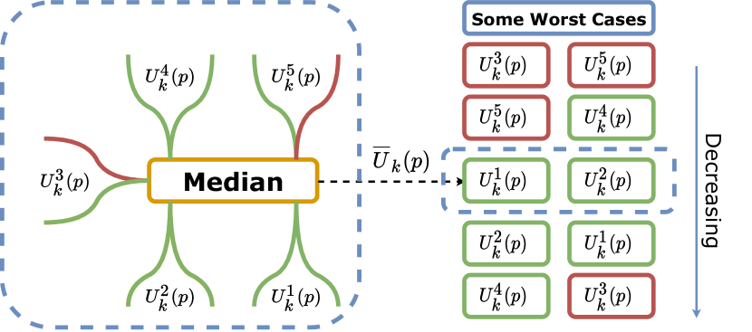
Figure 1: An exemplary scenario with ten clients where two are Byzantine (red lines), and they perform outlier attacks. Fed-MoM-UCB first divides the clients into five groups. In the worst case, the Byzantine clients are assigned to different groups and saturate their groups’ local updates. The saturation will not affect the median estimate in any scenario.

V Theoretical Analyses

V-A MoM Estimator Concentration

Our analysis hinges on the observation that with a proper choice of $\alpha(\lambda)$, we can ensure that at least half of the $G=\lceil\alpha(\lambda)M\rceil$ groups in any phase $p$ will consist of only honest clients (i.e., see Fig. 1). At the same time, we want each group to contain as many clients as possible to decrease the effect of local model heterogeneity (i.e., client sampling noise) on the estimates. In order to control the group size, we introduce the following generic mapping as in [72].

Definition 1.

Let $\alpha:[0,1/2]\rightarrow[0,1]$ be a mapping s.t.

$$\forall\lambda\in[0,1/2),~{}2\lambda<\alpha(\lambda)<1~{}.$$

Remark 1.

Notice that for a fixed mapping $\alpha(\lambda)$, the group size $B=\lfloor M/G\rfloor\leq M/(\alpha(\lambda)M)\leq 1/\alpha(\lambda)$ can not increase with $p$ as it is strictly upper-bounded by $1/\alpha(\lambda)$. As the number of clients in a group can not increase with $p$, the uncertainty emerging from the client sampling within a group does not decrease over phases, which carries out to the global estimates since the server uses a median-of-means estimator to pick a single group. This observation points out how partial identifiability presents itself in the MoMoM estimator. Moreover, this is precisely the reason we recruit all the clients once at the beginning.

The following lemma presents a concentration bound for the MoM estimate of a global arm outcome $\mu_{k}$ in a phase $p$.

Lemma 1.

(MoM concentration bound). Let $G=\lceil\alpha(\lambda)M\rceil$, $\eta(\lambda)\coloneqq(\alpha(\lambda)-\lambda)/\alpha(\lambda)$, and $\rho:=\sigma/\sqrt{s(p)}+\sigma_{c}$. We have,

$$\Pr\left\{|\overline{U}_{k}(p)-\mu_{k}|>\gamma_{p}\right\}\leq\exp\left(-\frac{2\eta(\lambda)-1}{16\rho^{2}}M\gamma_{p}^{2}\right)~{},$$ (8)

for all,

$$\gamma_{p}^{2}\geq 4\left(\frac{\sigma}{\sqrt{s(p)}}+\sigma_{c}\right)^{2}\left(\frac{4\eta(\lambda)-1}{2\eta(\lambda)-1}\frac{\log 2}{B}\right)~{}.$$ (9)

Proof.

The proof builds upon the proof of MoM concentration bound given in Proposition 2 of [72]. Remember that we have defined in Section III $\mathcal{M}$ as the client cohort with cardinality $\lvert\mathcal{M}\rvert=M$, and $\mathcal{M}^{\text{mal}}\subset\mathcal{M}$ as the set of Byzantine clients with cardinality $\lvert\mathcal{M}^{\text{mal}}\rvert=M^{\text{mal}}$. Let ${\mathcal{G}}_{p}$ denote the set of client groups formed by the server at the end of phase $p$ and ${\mathcal{G}}^{\text{tru}}_{p}\subseteq{\mathcal{G}}_{p}$ denote the subset of groups with no Byzantine clients. We denote by $G_{p}=\lvert{\mathcal{G}}_{p}\rvert$ and $G^{\text{tru}}_{p}:=|{\mathcal{G}}^{\text{tru}}_{p}|$ the cardinalities of these sets, respectively (i.e., the number of client groups within the sets). For the groups including even a single Byzantine client, we can not provide any concentration guarantee. The worst case is when each Byzantine client belongs to a different group, rendering the maximum number of clients unreliable. In such a case, at most $\lfloor\lambda M\rfloor$ of the $G_{p}$ groups will be corrupted by Byzantine clients, that is $M^{\text{mal}}\leq\lambda M$. Then, we have,

$$G^{\text{tru}}_{p}\geq G_{p}-\lambda M\geq G_{p}-\frac{\lambda G_{p}}{\alpha(\lambda)}~{}.$$

Fix $\gamma_{p}>0$. By definition of the sample median, if at least half of the groups have a sample mean estimate within $\gamma_{p}$-neighborhood of $\mu_{k}$, their sample median must be within $\gamma_{p}$-neighborhood of $\mu_{k}$ as well. We can then write,

$$\Pr(|\overline{U}_{k}(p)-\mu_{k}|>\gamma_{p}|{\mathcal{G}}_{p})$$

$$\leq\Pr\left(\sum_{i\in{\mathcal{G}}^{\text{tru}}_{p}}\mathbb{I}\{|U^{i}_{k}(p)-\mu_{k}|>\gamma_{p}\}\geq G^{\text{tru}}_{p}-G_{p}/2\bigg{|}{\mathcal{G}}_{p}\right)$$

$$\leq\Pr\left(\sum_{i\in{\mathcal{G}}^{\text{tru}}_{p}}\mathbb{I}\{|U^{i}_{k}(p)-\mu_{k}|>\gamma_{p}\}\geq\dfrac{2\eta(\lambda)-1}{2\eta(\lambda)}G^{\text{tru}}_{p}\bigg{|}{\mathcal{G}}_{p}\right)$$

$$\leq\sum_{g=\lceil\frac{2\eta(\lambda)-1}{2\eta(\lambda)}G_{p}^{\text{tru}}\rceil}^{G_{p}^{\text{tru}}}{G_{p}^{\text{tru}}\choose g}q_{p}^{g}(1-q_{p})^{G_{p}^{\text{tru}}-g}$$

$$\leq q_{p}^{\frac{2\eta(\lambda)-1}{2}G_{p}}2^{\eta(\lambda)G_{p}}~{},$$ (10)

where $q_{p}\coloneqq\Pr(|U^{i}_{k}(p)-\mu_{k}|>\gamma_{p}|{\mathcal{G}}_{p})$. (10) is derived as in the proof of Proposition 2 in [72] after observing that $\sum_{i\in{\mathcal{G}}^{\text{tru}}_{p}}\mathbb{I}\{|U^{i}_{k}(p)-\mu_{k}|>\gamma_{p}\}$ is a binomial random variable. Next, we observe the following for $i\in{\cal G}^{\text{tru}}_{p}$,

$$U^{i}_{k}(p)-\mu_{k}=\frac{1}{B}\sum_{m\in{\mathcal{B}}_{i,p}}(\widehat{\mu}_{m,k}(p)-\mu_{m,k}+\mu_{m,k}-\mu_{k})\\ =\underbrace{\frac{1}{B}\sum_{m\in{\mathcal{B}}_{i,p}}(\widehat{\mu}_{m,k}(p)-\mu_{m,k})}_{\text{Term I}}+\underbrace{\frac{1}{B}\sum_{m\in{\mathcal{B}}_{i,p}}(\mu_{m,k}-\mu_{k})}_{\text{Term II}}~{}.$$ (11)

By definition, Term I is the average of $B$ independent $\sigma/\sqrt{s(p)}$-subgaussian random variables. Thus, Term 1 is $\sigma/\sqrt{s(p)B}$-subgaussian. Similarly, Term 2 is the average of $B$ independent $\sigma_{c}$-subgaussian random variables. Therefore, it is $\sigma_{c}/\sqrt{B}$-subgaussian. As a result, Term I plus Term II is $\sigma/\sqrt{s(p)B}+\sigma_{c}/\sqrt{B}$-subgaussian. Let $\rho=\sigma/\sqrt{s(p)}+\sigma_{c}$ and $\rho^{\prime}\coloneqq\frac{1}{\sqrt{B}}\rho$. Then, using the subgaussian tail inequality (Theorem 5.3 in [73]), we have $q_{p}\leq 2e^{-\gamma_{p}^{2}/(2(\rho^{\prime})^{2})}=2e^{-B\frac{\gamma_{p}^{2}}{2\rho^{2}}}$. Plugging this into (10), we obtain,

$$\Pr (|\overline{U}_{k}(p)-\mu_{k}|>\gamma_{p})\leq\exp\left(-\frac{2\eta(\lambda)-1}{16\rho^{2}}M\gamma_{p}^{2}\right)~{},$$

for all,

$$\gamma_{p}^{2}\geq\frac{4\rho^{2}}{B}\frac{4\eta(\lambda)-1}{2\eta(\lambda)-1}\log 2~{},$$

which completes the proof. ∎

The MoM concentration bound in (8) conditional to (9) immediately gives the designer an insight towards the selection of the cohort size $M$ and the high probability confidence bound $E_{p}$ in (7). Note that as opposed to the case where $\overline{U}_{k}(p)$ (final estimator for $\mu_{k}$, see (5)) has subgaussian tail behavior, we can not provide any guarantees for an arbitrarily small confidence bound ($\gamma_{p}$ in (8)). The confidence bounds we can provide any guarantees for is strictly lower bounded by (9). It then follows that our best chance is to set (by (9)),

$$E_{p}=2\left(\underbrace{\frac{\sigma}{\sqrt{s(p)}}}_{\begin{subarray}{c}\text{arm}\\ \text{sampling}\end{subarray}}+\underbrace{\sigma_{c}}_{\begin{subarray}{c}\text{client}\\ \text{sampling}\end{subarray}}\right)\left(\frac{4\eta(\lambda)-1}{2\eta(\lambda)-1}\frac{\log 2}{B}\right)^{1/2}~{}.$$ (12)

Observe that no matter how many phases the algorithm iterates, the confidence bound we established in (12) can not shrink beyond an unavoidable margin determined in part by the local model heterogeneity level $\sigma_{c}$ (client sampling), which is formalized in Lemma 4. That happens because even though every single client continues collecting new observations over phases to decrease the uncertainty caused by the “arm sampling” in (12), we can not increase the number of clients within a group in which we “average” over as discussed in Remark 1. Next, by (8), we need to have,

$$\exp\left(-\frac{2\eta(\lambda)-1}{16\rho^{2}}ME_{p}^{2}\right)\leq\frac{\delta}{KT}~{},$$ (13)

to satisfy (7) for an arbitrary $\delta\in(0,1)$. Note that since we have $P_{T}\leq T$ and $\lvert{\cal A}_{p}\rvert\leq K$, ensuring that (13) holds implies that (7) holds after a union bound over all $p\in[P_{T}]$ and $k\in{\cal A}_{p}$. In the case where $\overline{U}_{k}(p)$ has subgaussian tail behavior, one could leverage employing more clients over phases (as in [3]) to maintain the high probability guarantees for a given $\delta\in(0,1)$ with a tighter confidence bound $E_{p}$. However, as we established in (12) by Lemma 1, our high probability confidence bound $E_{p}$ can shrink only so much in a given phase $p$. That is, employing more clients over phases does not provide us any advantage. Now, observe that in order to satisfy (13) after inserting $E_{p}$ as in (12), we must ensure,

$$M\geq\frac{4B\log(\frac{KT}{\delta})}{(4\eta(\lambda)-1)\log 2}~{}.$$

Since we have $B\leq 1/\alpha(\lambda)$ by Remark 1 and $M$ must be an integer, it suffices to have,

$$M=\frac{4\log(\frac{KT}{\delta})}{(4\eta(\lambda)-1)\alpha(\lambda)\log 2}+\Gamma_{1}~{},$$ (14)

for some constant $\Gamma_{1}\in[0,1)$. Finally, by (12) and (14), we can ensure that (7) holds for the tightest possible confidence bound $E_{p}$ using an MoM estimator, with probability at least $1-\delta$, for a given $\delta\in(0,1)$. For the rest of the manuscript, we always assume that the cohort size $M$ and the confidence bounds $E_{p}$ are set as in (12) and (14). Next, we define the “good event” where the confidence bounds hold over all phases and all active arms, and summarize our findings up to now in a single lemma.

Definition 2.

(Good event)

$${\cal E}\coloneqq\left\{\lvert\overline{U}_{k}(p)-\mu_{k}\rvert\leq E_{p},\forall p\in[P_{T}],\forall k\in\mathcal{A}_{p}\right\}~{}.$$ (15)

Lemma 2.

Pick $\delta\in(0,1)$ and a mapping $\alpha(\lambda)$ as in Definition 1. Set the cohort size $M$ as in (14) and the confidence bounds $E_{p}$ as in (12). We have,

$$\Pr\left\{{\cal E}\right\}\geq 1-\delta~{}.$$ (16)

Proof.

The proof simply reiterates over the results of our choices of the cohort size $M$ and the confidence bounds $E_{p}$. Observe that we have (13) by (12) and (14). Combining (13) with (8), we have,

$$\Pr\left\{|\overline{U}_{k}(p)-\mu_{k}|>E_{p}\right\}\leq\delta/KT~{}.$$ (17)

for any phase $p$ and arm $k$. Then,

$$\Pr \left\{|\overline{U}_{k}(p)-\mu_{k}|\leq E_{p},~{}\forall p\in[P_{T}],\forall k\in{\cal A}_{p}\right\}$$

$$\geq 1-\sum_{p\in[T]}\sum_{k\in[K]}\Pr\left\{|\overline{U}_{k}(p)-\mu_{k}|>E_{p}\right\}$$ (18)

$$\geq 1-\delta~{},$$ (19)

where (18) follows from the union bound and the fact that $P_{T}\leq T$ and $\lvert{\cal A}_{p}\rvert\leq K$. (19) then follows from (17). ∎

V-B Main Results and Regret Bound

By the end of each phase $p$, we execute the arm elimination rule in (6). We first show that the globally optimal arm $k^{*}\in[K]$ is guaranteed to always remain active.

Lemma 3.

Assume that the good event ${\cal E}$ in (15) holds. Then, the globally optimal arm $k^{*}$ is always guaranteed to remain active.

Proof.

For any phase $p$, let $k^{\prime}=\operatorname*{argmax}_{k\in{\cal A}_{p}}\{\overline{U}_{k}(p)\}$, that is, $k^{\prime}$ is empirically the best arm by the end of phase $p$. For the globally optimal $k^{*}$ to be eliminated by $k^{\prime}$, we need to have $\overline{U}_{k^{*}}(p)+E_{p}\leq\overline{U}_{k^{\prime}}(p)-E_{p}$ by (6). That implies,

$$\mu_{k^{*}} \leq\overline{U}_{k^{*}}(p)+E_{p}$$ (20)

$$\leq\overline{U}_{k^{\prime}}(p)-E_{p}$$

$$\leq\mu_{k^{\prime}}~{},$$ (21)

which is a contradiction since we have $\mu_{k^{*}}>\mu_{k^{\prime}}$. Note that we have (20) and (21) since the good event ${\cal E}$ holds. ∎

Lemma 3 have established that the globally optimal arm $k^{*}$ will never be eliminated under the good event ${\cal E}$. We utilize this fact to prove the elimination of $\beta$-suboptimal arms in the following lemmas. Fed-MoM-UCB employs uniform exploration combined with arm elimination. The following lemma first formalizes the unavoidable error margin $\omega$ which has been discussed in detail up to now in Sections III, V-A, and Remark 1. It then provides an upper bound on the number of phases required to eliminate a $\beta$-suboptimal arm.

Lemma 4.

($\beta$-suboptimal arm elimination) Following the “client sampling” term that is non-decreasing over phases in (12), we define the unavoidable error margin $\omega$ as,

$$\omega\coloneqq\frac{8\sigma_{c}\sqrt{\log 2}\sqrt{4\eta(\lambda)-1}}{\sqrt{B}\sqrt{2\eta(\lambda)-1}}~{}.$$ (22)

Then, under the good event ${\cal E}$, any arm $k\in[K]$ with suboptimality gap $\Delta_{k}>\omega$ will be eliminated by the end of phase $p_{k}$, where $p_{k}$ is the smallest integer satisfying

$$s(p_{k})\geq\frac{64\sigma^{2}\log 2(4\eta(\lambda)-1)}{(\Delta_{k}-\omega)^{2}B(2\eta(\lambda)-1)}~{}.$$ (23)

Since $\beta=\omega+\epsilon$, (23) holds for any $\beta$-suboptimal arm as well.

Proof.

Consider an $\omega$-suboptimal arm $k$, that is, $\Delta_{k}>\omega$. Furthermore, let $p_{k}$ be the smallest integer satisfying (23), which can be checked to imply $4E_{p_{k}}\leq\Delta_{k}$. Then, we have,

$$\overline{U}_{k}(p_{k})+E_{p_{k}} \leq\mu_{k}+2E_{p_{k}}$$ (24)

$$\leq\mu_{k}+2E_{p_{k}}+\overline{U}_{k^{*}}(p_{k})-\mu_{k^{*}}+E_{p_{k}}$$ (25)

$$=\overline{U}_{k^{*}}(p_{k})+3E_{p_{k}}-\Delta_{k}$$ (26)

$$\leq\overline{U}_{k^{*}}(p_{k})-E_{p_{k}}~{},$$ (27)

where (24) and (25) hold under the good event ${\cal E}$. (26) follows from the definition of the suboptimality gap $\Delta_{k}=\mu_{k^{*}}-\mu_{k}$, and (27) holds since we have $4E_{p_{k}}\leq\Delta_{k}$. Finally, by the arm elimination rule in (6), (27) then implies that an $\omega$-suboptimal arm $k$ will be eliminated at the end of phase $p_{k}$. ∎

Note that $p_{k}$ is the smallest integer satisfying (23). Then, we have,

$$s(p_{k})=\frac{64\sigma^{2}\log 2(4\eta(\lambda)-1)}{(\Delta_{k}-\omega)^{2}B(2\eta(\lambda)-1)}+\Gamma_{2}^{k}~{},$$ (28)

for some $\Gamma_{2}^{k}\geq 0$.

Remark 2.

Since $p_{k}$ has to be an integer, we have the additional constant $\Gamma_{2}^{k}\geq 0$, which depends on the suboptimality gap $\Delta_{k}$ of arm $k\in[K]$ and the choice of the mapping $s(p)$. For instance, if we choose $s(p)=a^{p}$ for some $a\in\{2,3,\ldots\}$, then the residual constant $\Gamma_{2}^{k}$ may be bigger compared to the choice $s(p)=ap$. The number of phases ($p_{k}$) required to eliminate a $\beta$-suboptimal arm is fewer in the former case since the clients collect more samples between phases, which increases the number of $\beta$-suboptimal arm pulls before they are eliminated (i.e., bigger $\Gamma_{2}^{k}$) and the cumulative regret. In the latter case, a $\beta$-suboptimal arm will be eliminated sooner (i.e., smaller $\Gamma_{2}^{k}$). However, that is at the cost of more frequent communication with the parameter server, which increases the cumulative regret through the communication cost. One edge case is $s(p)=p$, where a $\beta$-suboptimal arm $k$ will be eliminated “as soon as possible”, that is, $\Gamma_{2}^{k}=0$. In that case, the clients communicate with the parameter server every single time after they pull all the arms once. Another edge case is eliminating all the $\beta$-suboptimal arms in a single communication round, as we investigate in Corollary 1.

Lemma 4 forms the basis of the cumulative regret incurred by Fed-MoM-UCB by providing closed-form expressions for the phases where $\beta$-suboptimal arms will be eliminated. The following lemma ensures the elimination of all $\beta$-suboptimal arms.

Lemma 5.

(Termination) By the time Fed-MoM-UCB terminates, all the $\beta$-suboptimal arms are eliminated under the good event ${\cal E}$.

Proof.

Let us denote by $p_{\max}$ the phase after which Fed-MoM-UCB terminates, that is, $E_{p_{\max}}\leq\beta/4$ or $\lvert{\cal A}_{p_{\max}}\rvert=1$ by Algorithm 1. If the latter is the case, we have ${\cal A}_{p_{\max}}=\{k^{*}\}$ by Lemma 3 and we are done. For the former case where $E_{p_{\max}}\leq\beta/4$, remember that we have $\Delta_{k}>\beta$ for a $\beta$-suboptimal arm $k\in\neg{\cal K}_{\beta}$. Then, similar to the proof of Lemma 4, it immediately follows that,

$$\overline{U}_{k}(p_{\max})+E_{p_{\max}} \leq\overline{U}_{k^{*}}(p_{\max})+3E_{p_{\max}}-\Delta_{k}$$ (29)

$$\leq\overline{U}_{k^{*}}(p_{\max})-E_{p_{\max}}~{},$$ (30)

where (29) follows from (26), and (30) follows from $\Delta_{k}>\beta\geq 4E_{p_{\max}}$, suggesting that the $\beta$-suboptimal is bound to be eliminated by the end of phase $p_{\max}$. ∎

Before moving on to bounding the cumulative regret of Fed-MoM-UCB, we will derive an expression for $p_{\max}$ in Lemma 5, which will directly determine the upper bound on the total communication cost.

Lemma 6.

(Number of communication phases) Pick some $\epsilon~{}>~{}0$ to form $\beta=\omega+\epsilon$. Then, we have,

$$s(p_{\max})\leq\left\lceil\frac{64\sigma^{2}}{\epsilon^{2}}\left(\frac{4\eta(\lambda)-1}{2\eta(\lambda)-1}\frac{\log 2}{B}\right)\right\rceil~{},$$ (31)

where $\lceil x\rceil$ is the smallest integer greater than $x$.

Proof.

By our definitions of the unavoidable error margin $\omega$ (see (22)) and the confidence bounds $E_{p}$ (see (12)), we have,

$$E_{p}=\frac{\omega}{4}+\frac{2\sigma}{\sqrt{s(p)}}\left(\frac{4\eta(\lambda)-1}{2\eta(\lambda)-1}\frac{\log 2}{B}\right)^{1/2}~{}.$$ (32)

Remember that $\beta=\omega+\epsilon$, where $\epsilon>0$ can be chosen arbitrarily small. Fed-MoM-UCB stops the communication and arm elimination protocol when $E_{p}\leq\beta/4=(\omega+\epsilon)/4$. Let $p^{\prime}$ be the smallest integer satisfying,

$$\frac{2\sigma}{\sqrt{s(p^{\prime})}}\left(\frac{4\eta(\lambda)-1}{2\eta(\lambda)-1}\frac{\log 2}{B}\right)^{1/2}\leq\frac{\epsilon}{4}~{}.$$ (33)

Then, Fed-MoM-UCB is guaranteed to terminate at the end of phase $p^{\prime}$ by (32). Combining (33) with the fact that $p_{\max}\leq p^{\prime}$ and $s(p)$ is increasing in $p$, (31) follows. ∎

As one expects, the total number of phases increases for smaller $\epsilon$. Similar discussions to Remark 2 regarding effect of $s(p)$ on $p_{\max}$ follow as well. We also note that $p_{\max}\geq P_{T}$ in (3). We are now ready to bound the cumulative regret of Fed-MoM-UCB in (3). First, let us define the following constants to keep the notation uncluttered later.

Definition 3.

(Auxiliary constants)

$$\Gamma_{3} \coloneqq\frac{64\sigma^{2}(4\eta(\lambda)-1)\log 2}{(2\eta(\lambda)-1)B}~{}.$$ (34)

$$\Gamma_{4} \coloneqq\frac{4}{(4\eta(\lambda)-1)\alpha(\lambda)\log 2}~{}.$$ (35)

$$\Gamma_{5} \coloneqq\Gamma_{3}\Gamma_{4}~{}.$$ (36)

Theorem 1.

Pick $\delta\in(0,1)$ and $\epsilon>0$. Let $\lambda<0.5$ be the fraction of Byzantine clients and choose a mapping $\alpha(\lambda)$ satisfying Definition 1. Set $\beta=\omega+\epsilon$, the cohort size $M$ as in (14), and the confidence bounds $E_{p}$ as in (12). The cumulative regret of Fed-MoM-UCB can be upper-bounded as,

$$R^{\beta}_{T}<\sum_{k\in\neg\mathcal{K}_{\beta}} \left(\left(\frac{\Gamma_{5}}{\Delta_{k}-\omega}+\Gamma_{4}\Gamma_{2}^{k}(\Delta_{k}-\beta)\right)\log(\frac{KT}{\delta})\right.$$

$$\left.+\frac{\Gamma_{3}}{\Delta_{k}-\omega}+\Gamma_{2}^{k}(\Delta_{k}-\beta)\right)$$

$$+Cp_{\max}\left(\Gamma_{4}\log(\frac{KT}{\delta})+1\right)~{},$$ (37)

with probability at least $1-\delta$, where $p_{\max}$ satisfies (31).

Proof.

Given that a $\beta$-suboptimal arm $k\in\neg{\cal K}_{\beta}$ is bound to be eliminated by the end of the phase $p_{k}$, we have,

$$R^{\beta}_{T}\leq\sum_{k\in\neg\mathcal{K}_{\beta}}M(\Delta_{k}-\beta)s(p_{k})+CMp_{\max}~{},$$ (38)

By (28) and (34) we have,

$$(\Delta_{k}-\beta)s(p_{k}) =(\Delta_{k}-\beta)\left(\frac{\Gamma_{3}}{(\Delta_{k}-\omega)^{2}}+\Gamma^{2}_{k}\right)$$ (39)

$$<\frac{\Gamma_{3}}{\Delta_{k}-\omega}+\Gamma_{2}^{k}(\Delta_{k}-\beta)~{},$$ (40)

where (40) holds since $\beta>\omega$. Let us restate the expression for $M$ in (14) using (35),

$$M=\Gamma_{4}\log(\frac{KT}{\delta})+\Gamma_{1}~{},$$ (41)

where $\Gamma_{1}\in[0,1)$ is a constant. Theorem 1 then follows after combining (36), (38), (40), (41), and the fact that $\Gamma_{1}<1$. ∎

In the regret bound (37), the $\Gamma_{2}^{k}$ term multiplies the $\Delta_{k}-\beta$ term (i.e., instantaneous regret). This is inline with our observations in Remark 2, that is, a bigger residual $\Gamma_{2}^{k}$ will increase the regret. The $\Gamma_{5}/(\Delta_{k}-\omega)$ term intuitively suggests that a smaller suboptimality gap $\Delta_{k}$ will increase the regret as the suboptimal arm $k$ will remain active for a long time. Finally, the communication regret increases directly with smaller $\epsilon$ while also depending on the choice of $s(p)$ through $p_{\max}$. Note that one can explicitly find an upper bound on $p_{\max}$ via (31) for specific choices of $s(p)$.

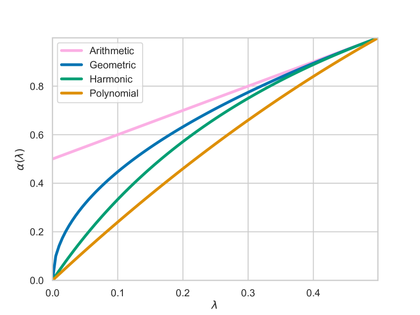
(a) $\lambda$ vs. $\alpha(\lambda)$

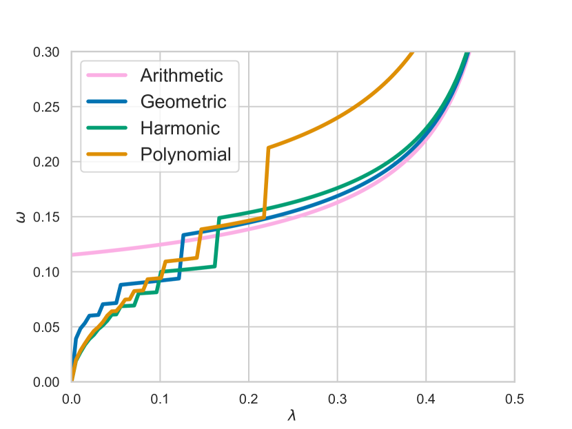
(b) $\lambda$ vs. $\omega$

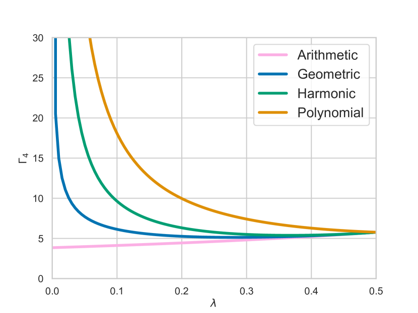
(c) $\lambda$ vs. $\Gamma_{4}$

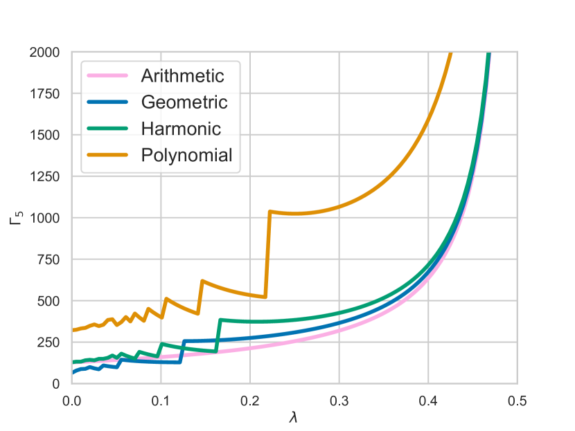
(d) $\lambda$ vs. $\Gamma_{5}$

Figure 2: The effect of Byzantine clients’ fraction $\lambda$ and the mapping $\alpha(\lambda)$ on the unavoidable error margin $\omega$, and the constants $\Gamma_{4}$ and $\Gamma_{5}$. The ladder structure occurs due to the dependence on the number of clients in a group, $B$, which is an integer. To draw the figures, we take $K=10$, $T=5\times 10^{4}$, $\delta=0.001$, $\sigma=0.5$, and $\sigma_{c}=0.01$.

Corollary 1.

It is possible to eliminate all $\beta$-suboptimal arms in a single communication round by choosing,

$$s(p)=\left\lceil\frac{\Gamma_{3}}{\epsilon^{2}}\right\rceil\times p~{},$$ (42)

in which case the cumulative regret can be upper bounded as,

$$R^{\beta}_{T}\leq\sum_{k\in\neg\mathcal{K}_{\beta}} (\Delta_{k}-\beta)\left(\Gamma_{4}\log(\frac{KT}{\delta})+1\right)\left(\frac{\Gamma_{3}}{\epsilon^{2}}+1\right)$$

$$+C\left(\Gamma_{4}\log(\frac{KT}{\delta})+1\right)~{},$$ (43)

Proof.

By (31), (34), and (42), we have $p_{\max}=1$ and $s(1)=\Gamma_{3}/\epsilon^{2}+\Gamma_{6}$ for some $\Gamma_{6}\in[0,1)$. Since $p_{k}=p_{\max}=1$ for all $k\in\neg{\cal K}_{\beta}$, the result follows from (38) and (41). ∎

Comparing $\eqref{eqn:correg}$ to (38), we see that even though a single round of communication is enough, the summation term on the right-hand side becomes bigger as $\Gamma_{3}/\epsilon^{2}+1\geq s(p_{k})$ for all $k\in\neg{\cal K}_{\beta}$. Note that the term governing the order of the cumulative regret with respect to the time horizon $T$ is the number cohort size $M$ (see (14)) by design. While different choices for $s(p)$ do not change the regret order in terms of the time horizon $T$, it determines the number of communication rounds before $\beta$-suboptimal arms are eliminated. Therefore, considering the communication cost and resources, the practitioner can choose a mapping $s(p)$ that suits the practical problem best.

V-C Choosing the mapping $\alpha(\lambda)$

The mapping $\alpha(\lambda)$ ensures that for a given $\lambda\in[0,0.5)$ fraction of Byzantine clients, we have sufficiently many distinct client groups to maintain robustness. This section investigates the effect of $\alpha(\lambda)$ on various parameters. Table I provides some different choices for $\alpha(\lambda)$ suggested in [72]. We are mainly interested in three important parameters directly affected by $\alpha(\lambda)$: the unavoidable error margin $\omega$, and the constants $\Gamma_{4}$ and $\Gamma_{5}$.

TABLE I: Different choices $\alpha(\lambda)$ satisfying Definition 1.

Mapping	$\rightarrow$	Arithmetic	Geometric	Harmonic	Polynomial
$\alpha(\lambda)$	$\rightarrow$	$(1+2\lambda)/2$	$\sqrt{2\lambda}$	$4\lambda(1+2\lambda)$	$\lambda(2.5-\lambda)$

Remark 1 briefly discussed the reason behind the unavoidable error margin $\omega$, which is the upper bound on the number of clients in a group ($B$) for a fixed upper bound on the Byzantine client fraction $\lambda$ and a mapping $\alpha(\lambda)$. The more clients we recruit, the more groups we need so that more than half of the groups will consist of honest clients only. Therefore, recruiting more clients do not help in increasing $B$. To maximize the number of clients in a group, however, one could argue choosing $\alpha(\lambda)$ as small as possible while satisfying Definition 1, such as $\alpha(\lambda)=2\lambda+\kappa$ for some arbitrarily small $\kappa>0$. Since the number of groups $G=\lceil\alpha(\lambda)M\rceil$ will be decrease with $\alpha(\lambda)$, we will have bigger groups as $B=\lfloor M/G\rfloor$. The unavoidable error margin $\omega$ in (22) decreases for a larger $B$ as expected. However, obtaining a larger $B$ is not free. Observe that $\omega$ in (22) also accommodates the the term,

$$\left(\frac{1}{2\eta(\lambda)-1}\right)^{2}=\left(\frac{\alpha(\lambda)}{\alpha(\lambda)-2\lambda}\right)^{2}~{},$$ (44)

since $\eta(\lambda)=(\alpha(\lambda)-\lambda)/\alpha(\lambda)$ (see Lemma 1). The r.h.s. in (44) goes to $+\infty$ as $\alpha(\lambda)\rightarrow 2\lambda$, exploding the unavoidable error $\omega$. That happens because although we have more crowded groups with smaller $\alpha(\lambda)$, we have fewer groups as well, which hurts our estimations since we use a median estimator over groups. In short, there is a tension between having more clients in a group to reduce the effect of client sampling and having more groups with fewer clients for better precision. Fig. 2(b) provides a guideline to choose the appropriate mapping to minimize the unavoidable error $\omega$. Comparing it to Fig. 2(a), we can confirm that a smaller choice for $\alpha(\lambda)$ is not the best option for a smaller $\omega$ in general.

Next, we investigate Figs. 2(c) and 2(d) to see how the constants $\Gamma_{4}$ and $\Gamma_{5}$ change with $\alpha(\lambda)$. Note that the constant $\Gamma_{4}$ determines the number of clients to be recruited, $M$, by (14). When the client recruitment is a bottleneck for the application, the practitioner should consider choosing $\alpha(\lambda)$ accordingly to obtain the desired performance with fewer clients. Moreover, the number of clients directly affects the cumulative regret as the arms will be played more before termination. Finally, we have $\Gamma_{5}=\Gamma_{3}\Gamma_{4}$ which scales the cumulative regret in (37). Observe that a bigger $\Gamma_{3}$ implies bigger confidence bounds, $E_{p}$, making eliminating the suboptimal arms harder and increasing the cumulative regret.

The choice of $\alpha(\lambda)$ determines the unavoidable error margin and the number of clients, and it also affects the cumulative regret. Therefore, choosing a suitable mapping that best fits a specific problem’s needs is crucial. In Section VI-C, we make experiments to investigate the effect of $\alpha(\lambda)$.

VI Experimental Results

In this section, we run simulations for a synthetic MAB problem with $K=10$ arms considering different attack schemes to test the Fed2-UCB and Fed-MoM-UCB algorithms’ performances. We present our results for three different scenarios. The main difference between the scenarios is the upper bound on the Byzantine clients’ fraction $\lambda$ and the attack structure. We explain our objectives and findings for each scenario in detail in the respective sections, and a comprehensive overview of the scenarios can be found in Table III. The unknown global mean arm outcomes $\mu_{k}$ for $k\in[10]$ are the same for all the scenarios and are given in Table II. The client and arm sampling uncertainties are modeled as zero-mean additive i.i.d. Gaussian noise with variances $\sigma_{c}^{2}=0.01^{2}$ and $\sigma^{2}=0.5^{2}$, respectively. We use $\delta=0.001$ and perform 100 independent experiments for each algorithm and scenario, and report the mean and standard deviations for the cumulative regret and the communication cost. We calculate the cumulative regret using (3) for both Fed2-UCB and Fed-MoM-UCB, where the $\beta$-optimal arms do not incur any regret.

TABLE II: Unknown global mean arm outcomes

$k$	$\rightarrow$	1	2	3	4	5	6	7	8	9	10
$\mu_{k}$	$\rightarrow$	0.4	0.5	0.55	0.6	0.65	0.7	0.75	0.8	0.85	0.95

VI-A Scenario 1

TABLE III: Parameters for different scenarios. The “M”, “B”, and “G” columns show the number of total clients recruited, the number of clients in a group, and the number of groups for the Fed-MoM-UCB algorithm, respectively. The “M(p)” and “M” columns show the number of clients recruited in phase $p$ and the number of total clients recruited by the Fed2-UCB algorithm, respectively. ($\pm$ standard deviation).

										Fed-MoM-UCB					Fed2-UCB
	T	$\lambda$	$\omega$	$\epsilon$	$\beta$	$\neg{\cal K}_{\beta}$	C	Attack		$\alpha(\lambda)$	M	B	G		M(p)	M
Scenario 1	$5\times 10^{4}$	0.2	0.139	0.05	0.189	$\{1,\ldots,7\}$	1	(45)		Arithmetic	89	1	89		10	$1237\pm 88$
															$2^{p}$	$16710\pm 2294$
Scenario 2	$10^{5}$	0.2	0.139	0.05	0.189	$\{1,\ldots,7\}$	0.1	(46)		Arithmetic	92	1	92		20	$1559\pm 120$
		0.25	0.149		0.199						96	1	96			$1277\pm 84$
Scenario 3	$5\times 10^{4}$	0.1	$\approx 0.1$	0.01	0.11	$\{1,\ldots,8\}$	0.1	(45)		Geometric	123	2	61		N/A	N/A
										Harmonic	193	2	96
										Polynomial	362	4	90

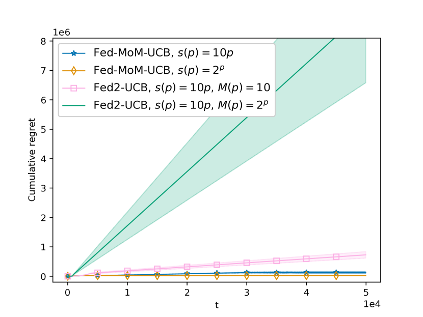
(a) Cumulative Regrets

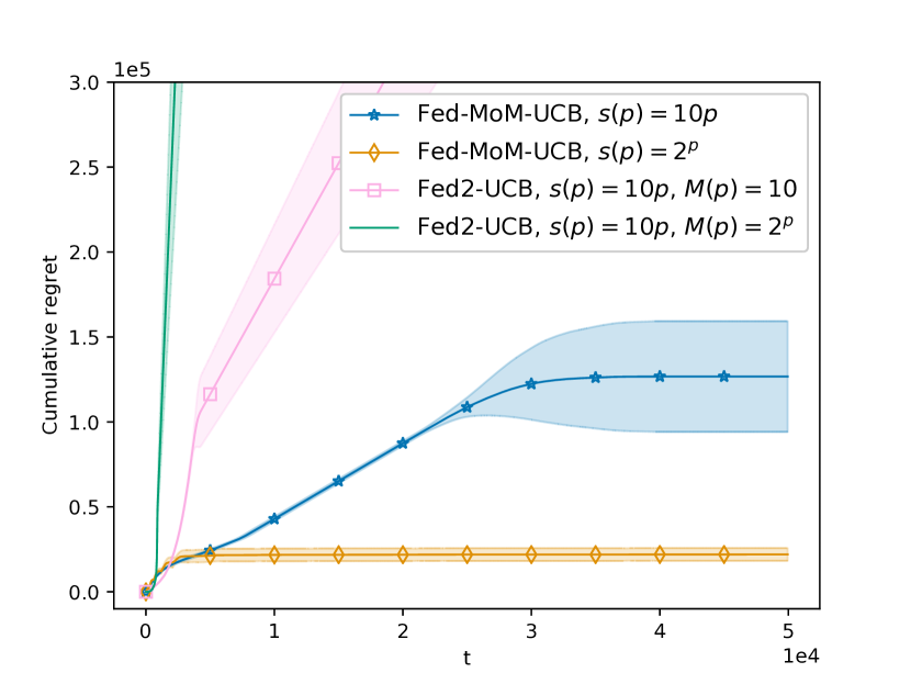
(b) Cumulative Regrets (zoomed)

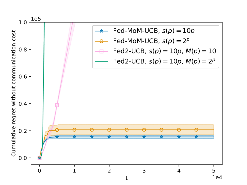
(c) Cumulative regrets without communication costs

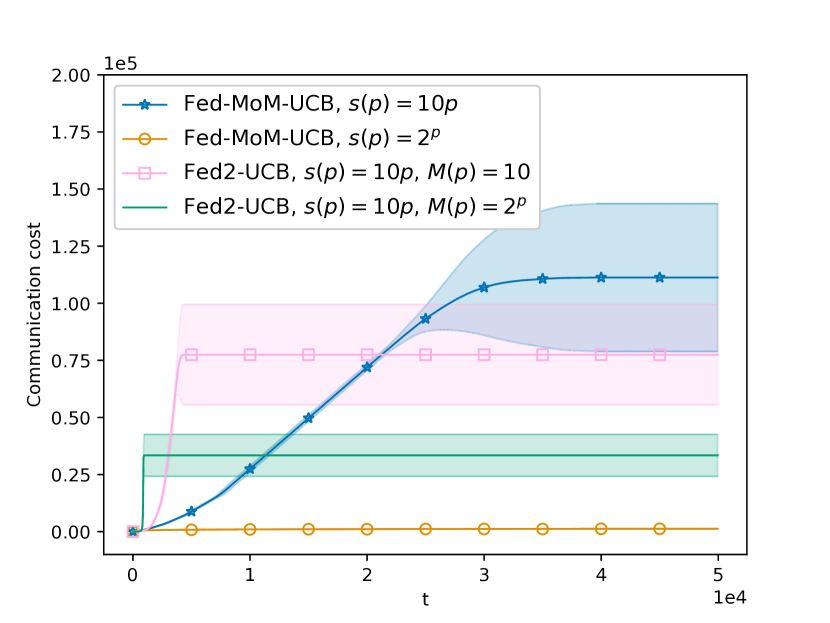
(d) Communication costs only

Figure 3: Cumulative regrets and communication costs for “Scenario 1” (with $\pm$ 2 standard deviation).

We set the Byzantine clients’ fraction to $\lambda=0.2$ and use the arithmetic mapping for Fed-MoM-UCB, that is, $\alpha(\lambda)=(1+2\lambda)/2$ (see Table I). We choose the arithmetic mapping as it yields the smallest value for the unavoidable error margin at $\lambda=0.2$, which is $\omega=0.139$ while also resulting in the smallest constants $\Gamma_{4}$ and $\Gamma_{5}$ that scale the number of clients to be recruited and the cumulative regret. We then set $\epsilon=0.05$ and obtain $\beta=0.189$. In that case, the $\beta$-suboptimal arm set is $\neg{\cal K}_{\beta}=\{1,\ldots,7\}$. The communication cost is set to $C=1$. Finally, we consider the following attack scheme for a Byzantine client $m$,

$$X_{m,k}(t)=\begin{dcases}\texttt{Unif}[0,~{}0.1]&\text{ if }k\in{\cal K}_{\beta}\\ \texttt{Unif}[0.9,~{}1]&\text{ if }k\in\neg{\cal K}_{\beta}\end{dcases}$$ (45)

where $X_{m,k}(t)$ denotes the local observation of the Byzantine client $m$ for the arm $k$ at round $t$. That is, a Byzantine client $m$ sets its local observations to a random value in $[0,~{}0.1]$ for the $\beta$-optimal arms and to a random value in $[0.9,~{}1]$ for the $\beta$-suboptimal arms, to make it harder for the parameter server to identify the $\beta$-optimal arms correctly.

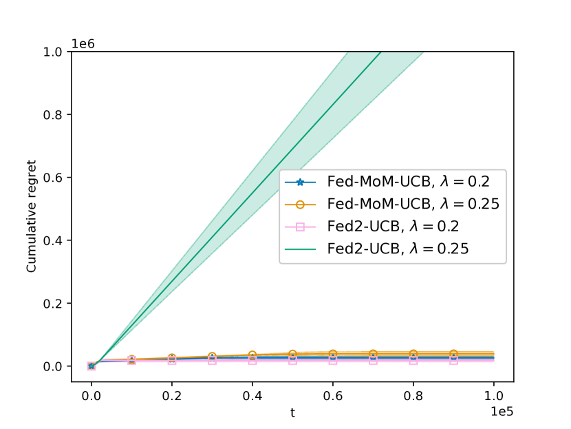
(a) Cumulative Regrets

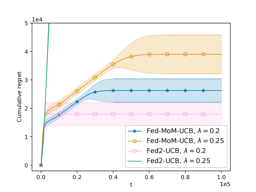
(b) Cumulative Regrets (zoomed)

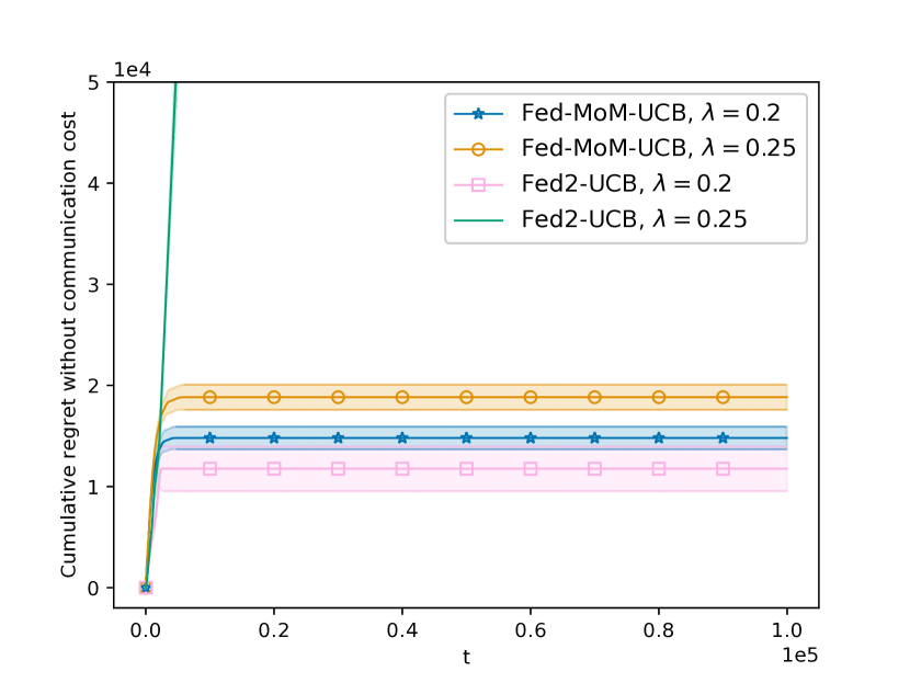
(c) Cumulative regrets without communication costs

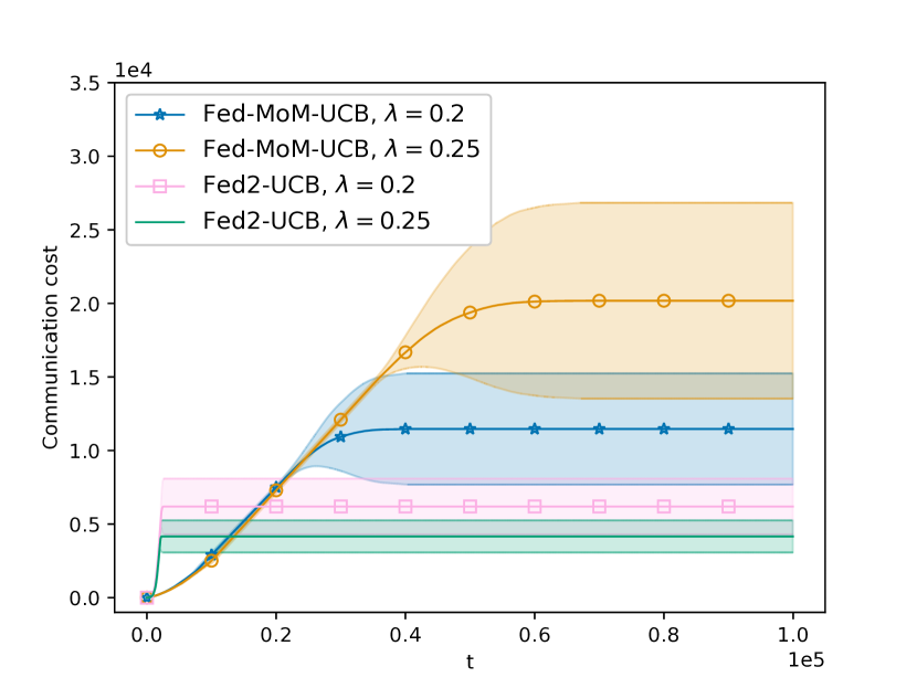
(d) Communication costs only

Figure 4: Cumulative regrets and communication costs for “Scenario 2” (with $\pm$ 2 standard deviation).

Unlike Fed-MoM-UCB, Fed2-UCB continues to recruit more clients over phases to reduce the uncertainty emerging from the client sampling. As discussed in Section V, that does not help in the presence of Byzantine clients. We set $s(p)=10p$ and run Fed2-UCB with two different configurations, $M(p)=10$ and $M(p)=2^{p}$, where $M(p)$ is the number of new clients recruited at phase $p$. Fig. 3(d) confirms that Fed2-UCB terminates. That is, only a single active arm is left, and the communication is stopped. However, the remaining arm is not a $\beta$-optimal arm since Fed2-UCB incurs linear regret in both cases as can be seen in Figs. 3(a) and 3(b). Moreover, while recruiting more clients does not help Fed2-UCB eliminate the $\beta$-suboptimal arms, the cumulative regret also explodes since the more new clients are recruited, the more the suboptimal arms are played. Table III shows the extreme difference between the total number of clients recruited by Fed2-UCB and by Fed-MoM-UCB when they terminate. The unlimited client recruitment scheme of Fed2-UCB does not only lead the cumulative regret to explode in the presence of Byzantine clients, but it may also not be feasible or even possible for some applications.

Fed-MoM-UCB recruits $M=89$ clients only once at the beginning and creates $G=89$ groups. In that case, Fed-MoM-UCB simply calculates the median of individual local updates for each arm at the parameter server. Note that even though it is possible to have $B=2$ as well while still maintaining the robustness, Fig. 2 suggests that the arithmetic mapping is the best option for $\lambda=0.2$. We run Fed-MoM-UCB with two different configurations, $s(p)=10p$ and $s(p)=2^{p}$. Fig. 3(d) confirms that Fed-MoM-UCB terminates and stops the communication in both cases. From Fig. 3(b), we can see that Fed-MoM-UCB is able to eliminate all the $\beta$-suboptimal arms as the cumulative regret ceases to increase. Moreover, as we discussed in Remark 2, the communication cost is extremely smaller for $s(p)=2^{p}$ compared to $s(p)=10p$. However, Fig. 3(c) shows that the cumulative regret is smaller for $s(p)=10p$ when the communication cost is not considered (i.e., $C=0$). That simply happens because the suboptimal arms are eliminated earlier for $s(p)=10p$ than $s(p)=2^{p}$ due to more frequent communication. The tradeoff between the communication cost and the regret incurred from playing the suboptimal arms is crucial, and it should be carefully treated depending on the application and the communication cost. While the overall cumulative regret is smaller with $s(p)=2^{p}$ as we can see in Fig. 3(b), it can be the other way around when the communication cost is smaller.

VI-B Scenario 2

In this part, we consider a very similar experimental setup to scenario 1, where we only change the attack scheme in (45). We also change the communication cost to $C=0.1$ to provide a more nuanced comparison through the plots in Fig. 4. We note that the difference in $M$ between scenarios 1 and 2 when $\lambda=0.2$ is due to the longer time horizon $T$. We consider the following attack scheme for a Byzantine client $m$,

$$X_{m,k}(t)=\begin{dcases}\texttt{Unif}[0,~{}0.1]&\text{ if }k\in{\cal K}_{\beta}\\ \mu_{m,k}+\zeta_{t}&\text{ if }k\in\neg{\cal K}_{\beta}\end{dcases}$$ (46)

That is, a Byzantine client $m$ sets its local observations to a random value in $[0,~{}0.1]$ for the $\beta$-optimal arms as in scenario 1, while recording honest samples for the $\beta$-suboptimal arms (see (1)). The attack scheme in (46) is milder than (45).

We experiment with two different values for the Byzantine client fraction, $\lambda=0.2$ and $\lambda=0.25$. Since the $\beta$-suboptimal arms are the same for both choices, we take $\beta=0.189$ while calculating the cumulative regret for a fair comparison between different settings and algorithms. For both cases, we run Fed2-UCB with $s(p)=10p$ and $M(p)=20$, and Fed-MoM-UCB for $s(p)=10p$. Fig. 4(d) confirms that all the algorithms terminates and the communication is stopped. When $\lambda=0.2$, we see that Fed2-UCB incurs lower cumulative regret than Fed-MoM-UCB in Fig. 4(a) and 4(b). While not completely, the difference in the performance partially depends on the regret incurred by the communication cost as hinted by Fig. 4(d). In Fig. 4(c), we see that Fed2-UCB’s and Fed-MoM-UCB’s cumulative regrets are closer when the communication cost is not considered. That happens because even though Fed-MoM-UCB eliminates all the suboptimal arms in practice and have the active arm set ${\cal A}_{p}=\{8,9,10\}$, which does not incur any additional regret, the communication continues unless either ${\cal A}_{p}=\{10\}$ or $E_{p}\leq\beta/4$. Since the confidence bounds (see (12)) used by the Fed-MoM-UCB accommodates a non-decreasing term (i.e., client sampling), it takes longer for Fed-MoM-UCB to terminate either by eliminating all the arms except the globally optimal arm (i.e., $k=10$), or by reducing the confidence bound to the point where $E_{p}\leq\beta/4$.

Finally, even though Fed2-UCB works well when $\lambda=0.2$, it fails when we increase the Byzantine client fraction to $\lambda=0.25$. Note that it still terminates and stops the communication when $\lambda=0.25$ as we see in Fig. 4(d). However, it eliminates all the $\beta$-optimal arms and settles on a $\beta$-suboptimal arm, incurring a linear regret as can be seen in Fig. 4(a). We remark that while Fed2-UCB may continue to work well under Byzantine attacks, slight changes to the attacking scheme or the fraction of the malicious clients can immediately render it ineffective. On the other hand, Fed-MoM-UCB can eliminate all the $\beta$-suboptimal arms when $\lambda=0.25$.

VI-C Scenario 3

In this part, we investigate how different choices for $\alpha(\lambda)$ affects the performance. We set the communication cost to $C=0.1$ and the Byzantine client fraction to $\lambda=0.1$. The attack scheme is the same as scenario 1 (see (45)).

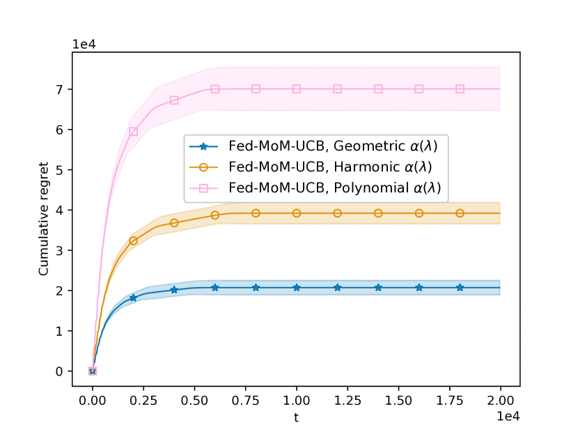
(a) Cumulative Regrets

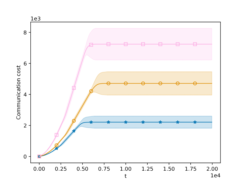
(b) Communication costs

Figure 5: Cumulative regrets and communication costs for “Scenario 3” (with $\pm$ 2 standard deviation).

We refer to Fig. 2 to decide on a mapping, $\alpha(\lambda)$. We first observe from Fig. 2(b) that the unavoidable error margin is very close for the geometric, harmonic, and polynomial mappings, which can be taken as $\omega\approx 0.1$. Then, Fig. 2(c) and 2(d) suggest that the best choice is the geometric mapping, as it results in the smallest constants $\Gamma_{4}$ and $\Gamma_{5}$, which scale the number of clients to be recruited and the cumulative regret. Similarly, the polynomial mapping seems to be the worst choice. To test our hypothesis, we run the Fed-MoM-UCB using all three candidate mappings. As Fig. 5(a) shows, the order between the cumulative regrets of the mappings is as expected. The geometric mapping offers the best performance with the minimum number of clients $M=123$, while the polynomial mapping offers the worst with the maximum number of clients $M=362$. As discussed in Section V-C, the choice of the mapping is crucial, and it affects a variety of parameters that may not be sufficient alone to decide the best mapping. The practitioner must carefully analyze the tradeoff between the unavoidable error margin $\omega$, the number of required clients $M$ (determined by $\Gamma_{4}$), and other constants which scale the cumulative regret before choosing a mapping.

VII Conclusion

We have proposed a robust median-of-means-based algorithm, Fed-MoM-UCB, to operate in a federated multi-armed bandit framework where Byzantine clients threaten the performance. We showed that when at most half the client pool consists of Byzantine clients, it is possible to maintain robustness and provide an upper bound on the cumulative regret while also considering the communication cost, a primary bottleneck of the federated learning systems. We showed that coping with the Byzantine clients via a median-based estimator comes at the cost of an unavoidable error margin caused by the non-increasing size of the client groups. We showed that recruiting more clients does not solve that problem, and we derived an expression for the required number of clients necessary to provide high probability guarantees on the cumulative regret. We thoroughly investigated the interplay between the different algorithm parameters and performance metrics. Finally, we compared Fed-MoM-UCB’s performance against Fed2-UCB’s and confirmed its effectiveness under Byzantine attacks. Interesting future work includes a detailed investigation on reducing the error margin emanating from client sampling while retaining robustness against adversaries.

References

- [1] R. S. Sutton, A. G. Barto et al., Introduction to Reinforcement Learning. MIT Press Cambridge, 1998.
- [2] T. L. Lai and H. Robbins, “Asymptotically efficient adaptive allocation rules,” Advances in Applied Mathematics, vol. 6, no. 1, pp. 4–22, 1985.
- [3] C. Shi and C. Shen, “Federated multi-armed bandits,” Proceedings of the AAAI Conference on Artificial Intelligence, vol. 35, no. 11, pp. 9603–9611, 2021.
- [4] L. Lamport, R. E. Shostak, and M. C. Pease, “The byzantine generals problem,” in Concurrency: The Works of Leslie Lamport, D. Malkhi, Ed., 2019, pp. 203–226.
- [5] H. B. McMahan, E. Moore, D. Ramage, and B. A. y Arcas, “Federated learning of deep networks using model averaging,” arXiv preprint arXiv:1602.05629, 2016.
- [6] K. Bonawitz, H. Eichner et al., “Towards federated learning at scale: System design,” in Proceedings of Machine Learning and Systems, vol. 1, 2019, pp. 374–388.
- [7] P. Kairouz, McMahan et al., “Advances and open problems in federated learning,” Foundations and Trends in Machine Learning, vol. 14, no. 1–2, pp. 1–210, 2021.
- [8] A. Vempaty, L. Tong, and P. K. Varshney, “Distributed inference with byzantine data: State-of-the-art review on data falsification attacks,” IEEE Signal Processing Magazine, vol. 30, no. 5, pp. 65–75, 2013.
- [9] Y. Chen, S. Kar, and J. M. Moura, “The internet of things: Secure distributed inference,” IEEE Signal Processing Magazine, vol. 35, no. 5, pp. 64–75, 2018.
- [10] B. Biggio, B. Nelson, and P. Laskov, “Poisoning attacks against support vector machines,” in International Conference on Machine Learning (ICML), 2012, pp. 1467–1474.
- [11] Y. Liu, S. Ma, Y. Aafer, W.-C. Lee, J. Zhai, W. Wang, and X. Zhang, “Trojaning attack on neural networks,” in Annual Network and Distributed System Security Symposium, 2017.
- [12] Y. Chen, S. Kar, and J. M. Moura, “Resilient distributed parameter estimation with heterogeneous data,” IEEE Trans. Signal Process, vol. 67, no. 19, pp. 4918–4933, 2019.
- [13] I. J. Goodfellow, J. Shlens, and C. Szegedy, “Explaining and harnessing adversarial examples,” in International Conference on Learning Representations (ICLR), 2015.
- [14] C. Szegedy, W. Zaremba et al., “Intriguing properties of neural networks,” in International Conference on Learning Representations (ICLR), 2014.
- [15] E. Bagdasaryan, A. Veit, Y. Hua, D. Estrin, and V. Shmatikov, “How to backdoor federated learning,” in International Conference on Artificial Intelligence and Statistics (AISTATS), vol. 108, 2020, pp. 2938–2948.
- [16] K. Pillutla, S. M. Kakade, and Z. Harchaoui, “Robust aggregation for federated learning,” IEEE Trans. Signal Process, vol. 70, pp. 1142–1154, 2022.
- [17] P. Blanchard, E. M. E. Mhamdi, R. Guerraoui, and J. Stainer, “Machine learning with adversaries: Byzantine tolerant gradient descent,” in Advances in Neural Information Processing Systems (NeurIPS), 2017.
- [18] A. N. Bhagoji, S. Chakraborty, P. Mittal, and S. Calo, “Analyzing federated learning through an adversarial lens,” in International Conference on Machine Learning (ICML), 2019, pp. 634–643.
- [19] L. Lyu, H. Yu, X. Ma, L. Sun, J. Zhao, Q. Yang, and P. S. Yu, “Privacy and robustness in federated learning: Attacks and defenses,” arXiv preprint arXiv:2012.06337, 2020.
- [20] Z. Wu, Q. Ling, T. Chen, and G. B. Giannakis, “Federated variance-reduced stochastic gradient descent with robustness to byzantine attacks,” IEEE Trans. Signal Process, vol. 68, pp. 4583–4596, 2020.
- [21] D. Yin, Y. Chen, R. Kannan, and P. Bartlett, “Byzantine-robust distributed learning: Towards optimal statistical rates,” in International Conference on Machine Learning (ICML), 2018, pp. 5650–5659.
- [22] R. Guerraoui, S. Rouault et al., “The hidden vulnerability of distributed learning in byzantium,” in International Conference on Machine Learning (ICML), 2018, pp. 3521–3530.
- [23] M. Fang, X. Cao, J. Jia, and N. Gong, “Local model poisoning attacks to Byzantine-Robust federated learning,” in USENIX Security Symposium, 2020, pp. 1605–1622.
- [24] M. Mozaffari-Kermani, S. Sur-Kolay, A. Raghunathan, and N. K. Jha, “Systematic poisoning attacks on and defenses for machine learning in healthcare,” IEEE J. Biomed. Health Inform., vol. 19, no. 6, pp. 1893–1905, 2014.
- [25] S. Shen, S. Tople, and P. Saxena, “Auror: Defending against poisoning attacks in collaborative deep learning systems,” in Annual Conference on Computer Security Applications, 2016, p. 508–519.
- [26] X. Wei and C. Shen, “Federated learning over noisy channels,” in IEEE International Conference on Communications (ICC), 2021, pp. 1–6.
- [27] T. Sery, N. Shlezinger, K. Cohen, and Y. C. Eldar, “Over-the-air federated learning from heterogeneous data,” IEEE Trans. Signal Process, vol. 69, pp. 3796–3811, 2021.
- [28] M. M. Amiri and D. Gündüz, “Federated learning over wireless fading channels,” IEEE Trans. Wireless Commun., vol. 19, no. 5, pp. 3546–3557, 2020.
- [29] W. R. Thompson, “On the likelihood that one unknown probability exceeds another in view of the evidence of two samples,” Biometrika, vol. 25, no. 3/4, pp. 285–294, 1933.
- [30] S. Agrawal and N. Goyal, “Analysis of thompson sampling for the multi-armed bandit problem,” in Conference on Learning Theory (COLT), 2012, pp. 39–1.
- [31] R. Agrawal, “Sample mean based index policies by o(log n) regret for the multi-armed bandit problem,” Advances in Applied Probability, vol. 27, no. 4, pp. 1054–1078, 1995.
- [32] P. Auer, N. Cesa-Bianchi, and P. Fischer, “Finite-time analysis of the multiarmed bandit problem,” Machine Learning, vol. 47, no. 2, pp. 235–256, 2002.
- [33] Y. Abbasi-Yadkori, D. Pál, and C. Szepesvári, “Improved algorithms for linear stochastic bandits,” Advances in Neural Information Processing Systems (NeurIPS), vol. 24, pp. 2312–2320, 2011.
- [34] S. Bubeck and N. Cesa-Bianchi, “Regret analysis of stochastic and nonstochastic multi-armed bandit problems,” Foundations and Trends in Machine Learning, vol. 5, no. 1, pp. 1–122, 2012.
- [35] A. Garivier and O. Cappé, “The kl-ucb algorithm for bounded stochastic bandits and beyond,” in Conference on Learning Theory (COLT), 2011, pp. 359–376.
- [36] N. Srinivas, A. Krause, S. M. Kakade, and M. W. Seeger, “Information-theoretic regret bounds for gaussian process optimization in the bandit setting,” IEEE Trans. Inf. Theory, vol. 58, no. 5, pp. 3250–3265, 2012.
- [37] W. Chu, L. Li, L. Reyzin, and R. Schapire, “Contextual bandits with linear payoff functions,” in International Conference on Artificial Intelligence and Statistics (AISTATS), 2011, pp. 208–214.
- [38] B. Kveton, C. Szepesvari, Z. Wen, and A. Ashkan, “Cascading bandits: Learning to rank in the cascade model,” in International Conference on Machine Learning (ICML), 2015, pp. 767–776.
- [39] Z. Wen, B. Kveton, M. Valko, and S. Vaswani, “Online influence maximization under independent cascade model with semi-bandit feedback,” in Advances in Neural Information Processing Systems (NeurIPS), 2017, pp. 3026–3036.
- [40] S. Vakili and Q. Zhao, “Risk-averse multi-armed bandit problems under mean-variance measure,” IEEE J. Sel. Topics Signal Process., vol. 10, no. 6, pp. 1093–1111, 2016.
- [41] X. Huo and F. Fu, “Risk-aware multi-armed bandit problem with application to portfolio selection,” Royal Society Open Science, vol. 4, no. 11, p. 171377, 2017.
- [42] K. Ding, J. Li, and H. Liu, “Interactive anomaly detection on attributed networks,” in ACM International Conference on Web Search and Data Mining, 2019, pp. 357–365.
- [43] V. Srivastava, P. Reverdy, and N. E. Leonard, “Surveillance in an abruptly changing world via multiarmed bandits,” in IEEE Conference on Decision and Control, 2014, pp. 692–697.
- [44] M. Y. Cheung, J. Leighton, and F. S. Hover, “Autonomous mobile acoustic relay positioning as a multi-armed bandit with switching costs,” in IEEE/RSJ International Conference on Intelligent Robots and Systems, 2013, pp. 3368–3373.
- [45] A. Anandkumar, N. Michael, A. K. Tang, and A. Swami, “Distributed algorithms for learning and cognitive medium access with logarithmic regret,” IEEE J. Sel. Areas Commun., vol. 29, no. 4, pp. 731–745, 2011.
- [46] S. S. Villar, J. Bowden, and J. Wason, “Multi-armed bandit models for the optimal design of clinical trials: benefits and challenges,” Statistical Science: A Review Journal of the Institute of Mathematical Statistics, vol. 30, no. 2, p. 199, 2015.
- [47] C. Shen, Z. Wang, S. Villar, and M. Van Der Schaar, “Learning for dose allocation in adaptive clinical trials with safety constraints,” in International Conference on Machine Learning (ICML), 2020, pp. 8730–8740.
- [48] K. Liu and Q. Zhao, “Decentralized multi-armed bandit with multiple distributed players,” in IEEE Information Theory and Applications Workshop (ITA), 2010, pp. 1–10.
- [49] ——, “Distributed learning in multi-armed bandit with multiple players,” IEEE Trans. Signal Process, vol. 58, no. 11, pp. 5667–5681, 2010.
- [50] A. Anandkumar, N. Michael, and A. Tang, “Opportunistic spectrum access with multiple users: Learning under competition,” in Proceedings of IEEE INFOCOM, 2010, pp. 1–9.
- [51] P. Landgren, V. Srivastava, and N. E. Leonard, “On distributed cooperative decision-making in multiarmed bandits,” in IEEE European Control Conference (ECC), 2016, pp. 243–248.
- [52] ——, “Social imitation in cooperative multiarmed bandits: Partition-based algorithms with strictly local information,” in IEEE Conference on Decision and Control (CDC), 2018, pp. 5239–5244.
- [53] D. Martínez-Rubio, V. Kanade, and P. Rebeschini, “Decentralized cooperative stochastic bandits,” Advances in Neural Information Processing Systems (NeurIPS), vol. 32, 2019.
- [54] Z. Zhu, J. Zhu, J. Liu, and Y. Liu, “Federated bandit: A gossiping approach,” in ACM SIGMETRICS/International Conference on Measurement and Modeling of Computer Systems, 2021, pp. 3–4.
- [55] S. Boyd, A. Ghosh, B. Prabhakar, and D. Shah, “Randomized gossip algorithms,” IEEE Trans. Inf. Theory, vol. 52, no. 6, pp. 2508–2530, 2006.
- [56] T. Li and L. Song, “Privacy-preserving communication-efficient federated multi-armed bandits,” IEEE J. Sel. Areas Commun., 2022.
- [57] A. Dubey and A. Pentland, “Differentially-private federated linear bandits,” Advances in Neural Information Processing Systems, (NeurIPS), vol. 33, pp. 6003–6014, 2020.
- [58] R. Huang, W. Wu, J. Yang, and C. Shen, “Federated linear contextual bandits,” Advances in Neural Information Processing Systems (NeurIPS), vol. 34, 2021.
- [59] P. Auer, N. Cesa-Bianchi, Y. Freund, and R. E. Schapire, “Gambling in a rigged casino: The adversarial multi-armed bandit problem,” in IEEE Annual Foundations of Computer Science, 1995, pp. 322–331.
- [60] K.-S. Jun, L. Li, Y. Ma, and J. Zhu, “Adversarial attacks on stochastic bandits,” Advances in Neural Information Processing Systems (NeurIPS), vol. 31, 2018.
- [61] F. Liu and N. Shroff, “Data poisoning attacks on stochastic bandits,” in International Conference on Machine Learning (ICML), 2019, pp. 4042–4050.
- [62] T. Lykouris, V. Mirrokni, and R. Paes Leme, “Stochastic bandits robust to adversarial corruptions,” in Proceedings of the 50th Annual ACM SIGACT Symposium on Theory of Computing, 2018, pp. 114–122.
- [63] A. Gupta, T. Koren, and K. Talwar, “Better algorithms for stochastic bandits with adversarial corruptions,” in Conference on Learning Theory (COLT), 2019, pp. 1562–1578.
- [64] I. Bogunovic, A. Krause, and J. Scarlett, “Corruption-tolerant gaussian process bandit optimization,” in International Conference on Artificial Intelligence and Statistics (AISTATS), 2020, pp. 1071–1081.
- [65] E. Garcelon, B. Roziere, L. Meunier, J. Tarbouriech, O. Teytaud, A. Lazaric, and M. Pirotta, “Adversarial attacks on linear contextual bandits,” Advances in Neural Information Processing Systems (NeurIPS), vol. 33, pp. 14 362–14 373, 2020.
- [66] I. Bogunovic, A. Losalka, A. Krause, and J. Scarlett, “Stochastic linear bandits robust to adversarial attacks,” in International Conference on Artificial Intelligence and Statistics (AISTATS), 2021, pp. 991–999.
- [67] J. Altschuler, V.-E. Brunel, and A. Malek, “Best arm identification for contaminated bandits,” Journal of Machine Learning Research, vol. 20, no. 91, pp. 1–39, 2019.
- [68] S. Bubeck, N. Cesa-Bianchi, and G. Lugosi, “Bandits with heavy tail,” IEEE Trans. Inf. Theory, vol. 59, no. 11, pp. 7711–7717, 2013.
- [69] A. Mitra, H. Hassani, and G. Pappas, “Exploiting heterogeneity in robust federated best-arm identification,” arXiv preprint arXiv:2109.05700, 2021.
- [70] D. Vial, S. Shakkottai, and R. Srikant, “Robust multi-agent multi-armed bandits,” in International Symposium on Theory, Algorithmic Foundations, and Protocol Design for Mobile Networks and Mobile Computing, 2021, pp. 161–170.
- [71] E. Even-Dar, S. Mannor, Y. Mansour, and S. Mahadevan, “Action elimination and stopping conditions for the multi-armed bandit and reinforcement learning problems.” Journal of Machine Learning Research, vol. 7, no. 6, 2006.
- [72] P. Laforgue, G. Staerman, and S. Clémençon, “Generalization bounds in the presence of outliers: a median-of-means study,” in International Conference on Machine Learning (ICML), 2021, pp. 5937–5947.
- [73] T. Lattimore and C. Szepesvári, Bandit Algorithms. Cambridge University Press, 2020.