Cluster expansion for a dilute hard sphere gas dynamics

Abstract

In BGSS2 , a cluster expansion method has been developed to study the fluctuations of the hard sphere dynamics around the Boltzmann equation. This method provides a precise control on the exponential moments of the empirical measure, from which the fluctuating Boltzmann equation and large deviation estimates have been deduced. The cluster expansion in BGSS2 was implemented at the level of the BBGKY hierarchy, which is a standard tool to investigate the deterministic dynamics Cercignani_Illner_Pulvirenti . In this paper, we introduce an alternative approach, in which the cluster expansion is applied directly on real trajectories of the particle system. This offers a fresh perspective on the study of the hard sphere dynamics in the low density limit, allowing to recover the results obtained in BGSS2 , and also to describe the actual clustering of particle trajectories.

I Introduction and presentation of the model

A gas can be modelled by a billiard made of hard spheres, moving in agreement with the laws of classical mechanics. Initially (at time $t=0$) the spheres are randomly and identically distributed according to a probability measure which is then transported by the flow of the deterministic dynamics (see (1)-(2) below). For a dilute gas, it has been shown in the seminal work of Lanford Lanford that when the average number of particles goes to infinity in the Boltzmann-Grad limit, the gas density converges towards a solution to the Boltzmann equation, at least for a short time. This work triggered a wave of developments, including some recent quantitative convergence results and generalisations to the case of compactly supported potentials; see spohn2012largeO ; Cercignani_Illner_Pulvirenti ; Cercignani_Gerasimenko_Petrina for surveys, and GSRT ; Pulvirenti_Saffirio_Simonella ; Pulvirenti_Simonella . In all these studies, the starting point is a system of evolution equations for the correlation functions, which are finite dimensional projections of the probability distribution assigned on the whole particle system. The $k$-particle correlation function $F_{k}\big{(}t,(x_{i},v_{i})_{i\leq k}\big{)}$ describes the distribution at time $t$ of $k$ typical particles with positions denoted by $x_{i}$ and velocities by $v_{i}$. These correlation functions obey the well known BBGKY hierarchy which states that, due to binary collisions, the variation in time of $F_{k}$ depends on the distribution of $k+1$ particles, $F_{k+1}$. As a consequence, the density of a typical particle $F_{1}$ does not follow a closed equation, and a substantial amount of work is required to prove that the correlation functions factorise in the Boltzmann-Grad limit, in such a way that the evolution equations can be closed with only the first limiting correlation function.

In the specific case of the billiard, the equations of the BBGKY hierarchy are singular and it is more convenient, mathematically, to represent the particle density in terms of an iterated Duhamel series (see e.g. Simonella_BBGKY ; GSRT on the justification of this series). This formula relates the density of a typical particle at time $t$, $F_{1}(t)$, to the initial probability measure (described by the collection $\left(F_{k}(0)\right)_{k\geq 1}$), by application of intertwined transport and collision operators. Ultimately this representation is studied by interpreting these chains of operators as integrals over so-called “pseudo-trajectories” (GSRT ), which play the role of a characteristic flow.

In BGSS2 , the analysis of the correlation functions has been improved in order to control the fluctuations of the empirical measure and not only its mean. The key feature is the computation of the precise asymptotics for the exponential moment of the empirical measure, which is done via a cumulant expansion. From this, several results can be derived, namely the fluctuating Boltzmann equation and the large deviations for the hard sphere gas. We refer to BGSS1 ; BGSS_ICM , and references therein, for a survey on these results and their physical interpretation, including the relation with stochastic particle dynamics (Kac process). One possible disadvantage of the iterated Duhamel representation is that the microscopic dynamics is not used directly, and the above-mentioned pseudo-trajectories do not correspond to physical trajectories. The link between the BBGKY hierarchy and physical trajectories is indeed very indirect (see for instance BGS_bigparticle , and Simonella_BBGKY ; Pulvirenti_Simonella_empirical ). Furthermore, the pseudo-trajectories are time-oriented, and followed backwards up to the initial time, which may appear to be at variance with the naive idea of a stochastic process.

The goal of the present paper is to obtain a statistical description of physical trajectories, without using the iterated Duhamel representation. More precisely, we will apply the cluster expansion method to real trajectories, controlling correlations of dynamical type. Cluster expansions have a long history in statistical mechanics, where they have been widely used to analyse correlations in Gibbs measures and the equilibrium behaviour of particle systems; see e.g. Ruelle_livre ; friedli2017statistical . Originally, they were designed to study gases in the low density regime and to establish thermodynamic relations in the spirit of the virial expansion. This powerful method was then proved to be effective in more general contexts, whenever relevant observables can be identified as weakly (or rarely) interacting. For example, for the Ising model in the phase transition regime, the relevant observables are no longer the spins, but the spin contours which form a dilute gas of contours at low temperature (friedli2017statistical ). More recently, the theory was extended to an abstract framework covering continuous particle systems and polymers poghosyan2009abstract . Several surveys have been written on the many aspects of the cluster expansion (which we do not quote exhaustively) and the topic has been matter of investigation for decades Brydges_course ; Kotecky_Preiss ; Gallavotti_Bonetto_Gentile ; Fernandez_Procacci ; Winter_Simonella ; Jansen_Kolesnikov .

In our approach, the elementary observable is not just the position (and velocity) of a classical particle, but rather the trajectory (or path) in $[0,T]$ of a “dynamical cluster” (see Figure 1 below). We show that for some short time $T>0$, the interactions are sufficiently rare so that the cluster expansion on such trajectories converges. Concerning correlations, the dynamical clusters studied in this paper play a similar role as the (perhaps more standard) cumulants, which were the main focus in BGSS2 : they grasp information on the dynamics on finer and finer scales. However, the cluster dynamics has an independent interest, when considering the problem of giving a mathematical meaning to the dynamics of the infinite system of particles (as obtained, for instance, from $N$ hard spheres in the Boltzmann-Grad limit). Indeed the cluster dynamics retains all the information on the limiting dynamics. The infinite system can be reinterpreted as a collection of clusters (groups of particles), moving independently and interacting randomly as in Sinai_cluster_1972 ; Sinai_cluster_1974 . The law of a typical cluster follows a coagulation process, the nonlinear behavior of which is reminiscent of Tanaka’s process for the Boltzmann equation Tanaka (see also Albeverio_Ruediger_Sunder_17 for space-dependent variants, and references therein). Our method provides a rigorous derivation of the limiting cluster process, Theorem IV.3.

We mention that dynamical clusters have been investigated previously, by means of numerical experiments on $N$ hard spheres Gabrielov_Keilis-Borok_Keilis-Borok_Zaliapin (see also McFadden_Bouchard ). The main focus of these simulations is a phase transition in the cluster formation process: a giant (macroscopic) cluster appears abruptly at a critical time. Later on in Patterson_Simonella_Wagner1 it was shown that, in the Boltzmann-Grad limit, the cluster dynamics can be described by explicit formulas and that in this limit, the critical transition takes place in times of order one. Finally in Patterson_Simonella_Wagner2 ; heydecker2019bilinear , the cluster process was studied for Kac particle systems, obtaining more precise results in spatially homogeneous cases. Theorem IV.3 below derives rigorously the cluster process from hard spheres, giving in particular a proof to the formal statements in Patterson_Simonella_Wagner1 , at least for short times.

Note that, contrary to Lanford’s approach which studies correlations for finite dimensional projections, the cluster expansion is implemented here directly on real paths of the full microscopic system – one will resort to projections only in a final step, in order to identify the Boltzmann equation for the limiting density (Section IV.1), or the asymptotics of the partition function governing the fluctuation theory and the large deviations (Section III.2). Compared to BGSS2 , this provides therefore an alternative take on the Boltzmann-Grad limit, with twofold interest: (i) a more direct link with physical trajectories; (ii) a representation of observables in terms of a forward-in-time process, with randomness entering through the initial measure. We refer also to Matthies-Theil ; Gerasimenko_Gapyak_21 for approaches sharing analogies with ours.

Let us now detail the model. We consider a microscopic system of identical hard spheres of unit mass and of diameter ${\varepsilon}$. The motion of $N$ such hard spheres is ruled by a system of ordinary differential equations, which are set in $({\mathbb{T}}^{d}\times\mathbb{R}^{d})^{N}$ where $\mathbb{T}^{d}=[0,1]^{d}$ is the unit $d$-dimensional periodic box with $d\geq 2$: writing ${\textbf{x}}^{{\varepsilon}}_{i}\in{\mathbb{T}}^{d}$ for the position of the center of the particle labeled by $i$ and ${\textbf{v}}^{{\varepsilon}}_{i}\in\mathbb{R}^{d}$ for its velocity, one has

$${d{\textbf{x}}^{{\varepsilon}}_{i}\over dt}={\textbf{v}}^{{\varepsilon}}_{i}\,,\quad{d{\textbf{v}}^{{\varepsilon}}_{i}\over dt}=0\quad\hbox{ as long as \ }|{\textbf{x}}^{{\varepsilon}}_{i}(t)-{\textbf{x}}^{{\varepsilon}}_{j}(t)|>{\varepsilon}\quad\hbox{for \ }1\leq i\neq j\leq N\,,$$ (1)

with specular reflection at collisions, i.e. when $|{\textbf{x}}^{{\varepsilon}}_{i}(t)-{\textbf{x}}^{{\varepsilon}}_{j}(t)|={\varepsilon}$

$$\begin{cases}\left({\textbf{v}}^{{\varepsilon}}_{i}\right)^{\prime}:={\textbf{v}}^{{\varepsilon}}_{i}-\big{(}({\textbf{v}}^{{\varepsilon}}_{i}-{\textbf{v}}^{{\varepsilon}}_{j})\cdot\boldsymbol{\omega}\big{)}\,\boldsymbol{\omega}\\ \left({\textbf{v}}^{{\varepsilon}}_{j}\right)^{\prime}:={\textbf{v}}^{{\varepsilon}}_{j}+\big{(}({\textbf{v}}^{{\varepsilon}}_{i}-{\textbf{v}}^{{\varepsilon}}_{j})\cdot\boldsymbol{\omega}\big{)}\,\boldsymbol{\omega}\end{cases}$$ (2)

where $\boldsymbol{\omega}:=({\textbf{x}}^{{\varepsilon}}_{i}(t)-{\textbf{x}}^{{\varepsilon}}_{j}(t))/{\varepsilon}$ is the unit vector pointing along the relative position at the collision time $t$. The collections of $N$ positions and velocities are denoted respectively by $X_{N}:=(x_{1},\dots,x_{N})$ in ${\mathbb{T}}^{dN}$ and $V_{N}:=(v_{1},\dots,v_{N})$ in $\mathbb{R}^{dN}$, and we set $Z_{N}:=(X_{N},V_{N})$, with $Z_{N}=(z_{1},\dots,z_{N})$, $z_{i}=(x_{i},v_{i})$. A set of $N$ particles is characterised by the time-zero configuration ${\textbf{Z}}^{{\varepsilon}0}_{N}=({\textbf{z}}^{{\varepsilon}0}_{1},\dots,{\textbf{z}}^{{\varepsilon}0}_{N})$ in the phase space

$${\mathcal{D}}^{{\varepsilon}}_{N}:=\big{\{}Z_{N}\in({\mathbb{T}}^{d}\times\mathbb{R}^{d})^{N}\,/\,\forall i\neq j\,,\quad|x_{i}-x_{j}|>{\varepsilon}\big{\}}\,,$$ (3)

and an evolution

$$t\mapsto{\textbf{Z}}^{{\varepsilon}}_{N}(t)=\big{(}{\textbf{z}}^{{\varepsilon}}_{1}(t),\dots,{\textbf{z}}^{{\varepsilon}}_{N}(t)\big{)}\;,\qquad t>0$$

according to the flow (1)-(2) (well defined almost surely under the Lebesgue measure Alexander ).

The dynamics is deterministic, but the initial data are chosen randomly according to the grand canonical formalism described below (see Ruelle_livre for details). The number of particles $\mathcal{N}$ is a random variable so that the initial measure is defined on the phase space

$$\mathcal{D}^{\varepsilon}:=\bigcup_{N\geq 0}\mathcal{D}^{\varepsilon}_{N}$$

(notice that $\mathcal{D}^{\varepsilon}_{N}=\emptyset$ for $N$ large due to the exclusion condition). Initially, the probability density of finding $N$ particles with configuration $Z_{N}$ is given by

$$\frac{1}{N!}W^{{\varepsilon}}_{N}(Z_{N}):=\frac{1}{\mathcal{Z}^{\varepsilon}}\,\frac{\mu_{\varepsilon}^{N}}{N!}\,{\textbf{1}}_{{\mathcal{D}}^{{\varepsilon}}_{N}}(Z_{N})\;\prod_{i=1}^{N}f^{0}(z_{i})\,,$$ (4)

where the distribution of a single particle $f^{0}$ is a Lipschitz continuous probability density on ${\mathbb{T}}^{d}\times\mathbb{R}^{d}$ satisfying the following bound for some constants $\beta,C_{0}>0$

$$\forall z\in{\mathbb{T}}^{d}\times\mathbb{R}^{d},\quad f^{0}(z)\leq C_{0}\mathcal{M}_{\beta}(v)\quad\text{with}\quad\mathcal{M}_{\beta}(v):=\frac{\beta^{d/2}}{(2\pi)^{\frac{d}{2}}}\exp\left(-\beta\frac{|v|^{2}}{2}\right),$$ (5)

and the partition function is given by

$$\mathcal{Z}^{\varepsilon}:=1+\sum_{N\geq 1}\frac{\mu_{\varepsilon}^{N}}{N!}\int_{\mathcal{D}^{\varepsilon}_{N}}dZ_{N}\prod_{i=1}^{N}f^{0}(z_{i})\,.$$ (6)

The stated assumptions on the initial measure will be kept throughout all the paper. The probability of an event $A$ with respect to the measure (4) will be denoted ${\mathbb{P}}_{\varepsilon}(A)$, and ${\mathbb{E}}_{\varepsilon}$ will be the expectation.

In the low density regime, referred to as the Boltzmann-Grad scaling, the expectation of the number of particles $\mathcal{N}$ is tuned by the parameter

$$\mu_{\varepsilon}:={\varepsilon}^{-(d-1)},$$ (7)

ensuring that the mean free path between collisions is of order one Grad49 . Definition (4) implies that

$$\lim_{{\varepsilon}\to 0}\;\mu_{\varepsilon}^{-1}{\mathbb{E}}_{\varepsilon}\left(\mathcal{N}\right)=1.$$

Let us denote by $W^{{\varepsilon}}_{N}(t,Z_{N})$ the probability density of finding $N$ particles with configuration $Z_{N}$ at time $t$, which satisfies the Liouville equation

$$\partial_{t}W^{{\varepsilon}}_{N}+V_{N}\cdot\nabla_{X_{N}}W^{{\varepsilon}}_{N}=0\,\,\,\,\,\,\,\,\,\hbox{on }\,\,\,{\mathcal{D}}^{{\varepsilon}}_{N}\,,$$ (8)

with specular reflection on the boundary. The $k$-th correlation function is defined by

$$F_{k}^{{\varepsilon}}(t,Z_{k}):=\mu_{\varepsilon}^{-k}\,\sum_{p=0}^{\infty}\,\frac{1}{p!}\,\int dz_{k+1}\dots dz_{k+p}\,W_{k+p}^{{\varepsilon}}(t,Z_{k+p})$$

and as mentioned earlier in the introduction, the key result originally derived by Lanford Lanford is the convergence of $F_{k}^{{\varepsilon}}$ to the tensor product $f^{\otimes k}$ where $f$ is the solution of the Boltzmann equation with initial data $f^{0}$

$$\left\{\begin{aligned} &\partial_{t}f+v\cdot\nabla_{x}f=\!\displaystyle\int_{\mathbb{R}^{d}}\int_{{\mathbb{S}}^{d-1}}\!\Big{(}f(t,x,w^{\prime})f(t,x,v^{\prime})-f(t,x,w)f(t,x,v)\Big{)}\big{(}(v-w)\cdot\omega\big{)}_{+}\,d\omega\,dw\,,\\ &f(0,x,v)=f^{0}(x,v)\end{aligned}\right.$$ (9)

with precollisional velocities $(v^{\prime},w^{\prime})$ defined by the scattering law

$$v^{\prime}:=v-\big{(}(v-w)\cdot\omega\big{)}\,\omega\,,\qquad w^{\prime}:=w+\big{(}(v-w)\cdot\omega\big{)}\,\omega\,.$$ (10)

This can be rephrased in terms of the convergence of the empirical density

$$\pi^{{\varepsilon}}_{t}:=\frac{1}{\mu_{\varepsilon}}\sum_{i=1}^{\mathcal{N}}\delta_{{\textbf{z}}^{\varepsilon}_{i}(t)}\;.$$ (11)

The convergence of the particle system to the Boltzmann equation can indeed be understood as follows.

Theorem I.1 (Lanford, Lanford )

There exists a time $T_{L}>0$ such that for any test function $h:{\mathbb{T}}^{d}\times\mathbb{R}^{d}\to\mathbb{R}$, any $\delta>0$ and $t\in[0,T_{L}]$,

$$\mathbb{P}_{\varepsilon}\left(\Big{|}\pi^{\varepsilon}_{t}(h)-\int_{{\mathbb{T}}^{d}\times\mathbb{R}^{d}}dzf(t,z)h(z)\Big{|}>\delta\right)\xrightarrow[\mu_{\varepsilon}\to\infty]{}0\,.$$ (12)

The time $T_{L}$ depends only on the smooth function $f^{0}$ through the constants $C_{0}$ and $\beta$ appearing in (5).

Notice that stronger convergence statements can be found IP89 ; Cercignani_Gerasimenko_Petrina ; Cercignani_Illner_Pulvirenti ; GSRT ; Pulvirenti_Simonella ; denlinger ; BGSS ; Gerasimenko_Gapyak_18 ; Gerasimenko_Gapyak_20 . All these studies rely on the BBGKY hierarchy and one of the goals of this paper is to provide an alternative derivation of Theorem I.1 by applying directly a cluster expansion at the level of the particle system. More generally, we are interested in the whole path of particle trajectories during a given time interval $[0,T]$. Let $\mathbb{D}([0,T],{\mathbb{T}}^{d}\times\mathbb{R}^{d})$ be the set of single particle trajectories ${\textbf{z}}^{\varepsilon}([0,T])$, which are functions piecewise linear continuous in position and piecewise constant in velocity. Then the generalised empirical measure is defined by

$$\pi^{{\varepsilon}}_{[0,T]}:=\frac{1}{\mu_{\varepsilon}}\sum_{i=1}^{\mathcal{N}}\delta_{{\textbf{z}}^{\varepsilon}_{i}([0,T])}\;.$$ (13)

To derive sharp estimates on the empirical measure, it is key to control its exponential moments, i.e. the Laplace transform

$$\widetilde{\Lambda}^{\varepsilon}_{T}(e^{h}):=\frac{1}{\mu_{\varepsilon}}\log\mathbb{E}_{\varepsilon}\left[\exp\Big{(}\mu_{\varepsilon}\,\pi^{\varepsilon}_{[0,T]}(h)\Big{)}\right]=\frac{1}{\mu_{\varepsilon}}\log\mathbb{E}_{\varepsilon}\Big{[}\exp\big{(}\sum_{i=1}^{\mathcal{N}}h\big{(}{\textbf{z}}^{{\varepsilon}}_{i}([0,T])\big{)}\big{)}\Big{]}\,,$$ (14)

for test functions $h:\mathbb{D}([0,T],{\mathbb{T}}^{d}\times\mathbb{R}^{d})\to\mathbb{C}$ measuring information on a single particle trajectory ${\textbf{z}}^{\varepsilon}([0,T])$. Indeed, it is well known in probability theory that the large deviations can be related to the Legendre transform of $h\mapsto\widetilde{\Lambda}^{\varepsilon}_{T}(e^{h})$ and that the fluctuations are coded by the characteristic function which amounts to considering functions $h$ of size $O(\mu_{\varepsilon}^{-\frac{1}{2}})$ with imaginary values. We refer to BGSS2 ; BGSS1 for the derivation of the fluctuating Boltzmann equation and of the large deviations once the asymptotic behaviour of $\widetilde{\Lambda}^{\varepsilon}_{T}$ has been characterised.

In the rest of this paper, we first analyse, in Section II, several types of dynamical interactions and show that the static cluster expansion on equilibrium measures can be extended to a dynamical cluster expansion in the dilute regime. Then we study its Boltzmann-Grad limit in Section III. Section IV is devoted to the derivation of limiting dynamical equations, including the Boltzmann equation as in Theorem I.1, and a coagulation-type equation driving the evolution of the dynamical clusters (Theorem IV.3).

II Dynamical cluster expansion

II.1 Decomposition in cluster paths

Throughout this section, we study the hard sphere dynamics on a fixed time interval $[0,T]$ and implement a cluster expansion to study the functional (14) as well as a natural extension which will be introduced in (21). This corresponds to a rather standard statistical mechanics computation, if not for the fact that the positions of classical particles are now replaced by their paths. Even though the gas is extremely dilute in the Boltzmann-Grad asymptotics, particles are likely to interact dynamically. In this case their trajectories are strongly modified by scattering. Thus to implement the dynamical cluster expansion, a good point of view is to first group particles which undergo collisions during $[0,T]$ and then to perform the standard cluster expansion on these groups of particles.

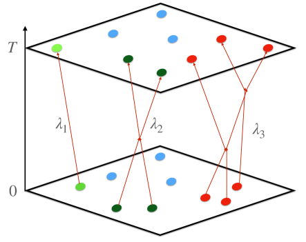
Figure 1: On this figure, three ${\varepsilon}$-cluster paths $\lambda_{1},\lambda_{2},\lambda_{3}$ are depicted in the time interval $[0,T]$. They are formed by groups of particles interacting dynamically. As the ${\varepsilon}$-cluster paths do not intersect, the trajectories within an ${\varepsilon}$-cluster path are only determined by the hard sphere dynamics restricted to the particles in this cluster path. Note that the other blue particles will form more cluster paths which have not been represented.

Definition II.1 (${\varepsilon}$-cluster path)

We say that two particles interact dynamically on $[0,T]$ if they collide on that time interval. Given a set of particle trajectories, a graph of dynamical interactions is built by adding an edge $\{i,j\}$ if two particles $i$ and $j$ from that set interact dynamically on $[0,T]$.

An ${\varepsilon}$-cluster path $\lambda$ on $[0,T]$ is a set $\{{\textbf{z}}^{\varepsilon}_{i}([0,T])\}_{i\in I_{\lambda}}$ of particle trajectories having a connected graph of dynamical interactions, and which do not interact dynamically with particles outside that set. The number of particles in the ${\varepsilon}$-cluster path $\lambda$ is denoted by $|\lambda|:=|I_{\lambda}|$.

Remark II.2

As the hard sphere dynamics is deterministic, the dynamical condition to form the ${\varepsilon}$-cluster path $\lambda$ on $[0,T]$ is coded in the initial data.

By definition, particles in an ${\varepsilon}$-cluster path $\lambda$ never collide with particles which do not belong to $\lambda$. Thus if a trajectory of the whole microscopic system ${\textbf{Z}}^{\varepsilon}_{N}([0,T])$ is decomposed into a partition $\{\lambda_{1},\dots,\lambda_{k}\}$ of ${\varepsilon}$-cluster paths, then particles in different cluster paths $\lambda_{i},\lambda_{j}$ do not collide. This condition is denoted by $\lambda_{i}\not\sim_{\varepsilon}\lambda_{j}$. Given the time interval $[0,T]$, the decomposition of ${\textbf{Z}}^{\varepsilon}_{N}([0,T])$ into ${\varepsilon}$-cluster paths is unique (see Figure 1). Note that the total kinetic energy of an ${\varepsilon}$-cluster path $\lambda_{j}$ is time independent within the time of existence of the path: $\displaystyle{\mathcal{E}}_{\lambda_{j}}:=\frac{1}{2}\sum_{i\in I_{\lambda_{j}}}|v^{\varepsilon}_{i}(t)|^{2}$ does not depend on $t\in[0,T]$.

By Definition II.1, given a time $T>0$, one has the following partition of unity

$${\textbf{1}}_{\mathcal{D}^{\varepsilon}_{N}}=\sum_{k\leq N}\sum_{\{\lambda_{1},\dots,\lambda_{k}\}\in\mathcal{P}_{{\textbf{Z}}^{\varepsilon}_{N}}^{k}}\left(\prod_{j\neq j^{\prime}}{\textbf{1}}_{\lambda_{j}\not\sim_{\varepsilon}\lambda_{j^{\prime}}}\right)\left(\prod_{j=1}^{k}{\textbf{1}}_{{\lambda_{j}}\hbox{ \scriptsize${\varepsilon}$-cluster path }}\right),$$ (15)

where $\mathcal{P}_{{\textbf{Z}}^{\varepsilon}_{N}}^{k}$ is the set of partitions of the single particle trajectories $({\textbf{z}}^{\varepsilon}_{i}([0,T]))_{i\leq N}$ into $k$ sets. We stress that, in formula (15), the ${\varepsilon}$-cluster paths are seen as functions of the initial (time-zero) configuration $\left(z_{i}\right)_{i\in I_{\lambda_{j}}}$.

This formula with the dynamical exclusion $\prod_{j\neq j^{\prime}}{\textbf{1}}_{\lambda_{j}\not\sim_{\varepsilon}\lambda_{j^{\prime}}}$ suggests to consider the system as a gas of ${\varepsilon}$-cluster paths. We expect this gas to be in a dilute regime for small times (roughly of the order of the convergence time $T_{L}$ introduced in Theorem I.1). The main results of this paper will actually be obtained by applying classical cluster expansions to this gas of ${\varepsilon}$-cluster paths.

We indicate by ${\textbf{Z}}:={\textbf{Z}}([0,T])$ a generic trajectory of size $|{\textbf{Z}}|:=n$, namely any element of ${\mathbb{D}}^{n}([0,T],{\mathbb{T}}^{d}\times{\mathbb{R}}^{d})$. Dropping the dependence on $T$ when there is no ambiguity, we have that ${\textbf{Z}}=\left\{{\textbf{z}}_{i}([0,T])\right\}_{i\leq n}$, and we assume that the trajectory conserves the total kinetic energy, meaning $\mathcal{E}_{\textbf{Z}}\displaystyle:=\frac{1}{2}\sum_{i\leq n}|{\textbf{v}}_{i}(t)|^{2}$ does not depend on $t\in[0,T]$. We equip the set of trajectories with the following norm: a sequence of trajectories ${\textbf{Z}}^{\ell}$ converges to a trajectory Z as $\ell$ goes to infinity if $|{\textbf{Z}}^{\ell}|=|{\textbf{Z}}|$ for $\ell$ large and

$$\|{\textbf{Z}}^{\ell}-{\textbf{Z}}\|_{T}:=\sup_{t\in[0,T]}\,\sup_{i\leq|{\textbf{Z}}|}\big{|}{\textbf{z}}^{\ell}_{i}(t)-{\textbf{z}}_{i}(t)\big{|}\xrightarrow[\ell\to\infty]{}0\;.$$ (16)

Let us now consider a complex-valued test function $H$ defined on the set of trajectories, such that the following bound holds uniformly over trajectories conserving the total kinetic energy

$$\left|H({\textbf{Z}})\right|\leq c_{1}|{\textbf{Z}}|+c_{2}\mathcal{E}_{\textbf{Z}}\quad\text{for some fixed constants $c_{1}>0$, \quad$0<c_{2}\leq\beta/4$}\,,$$ (17)

where we recall that $|{\textbf{Z}}|=n$ indicates the total number of particles involved in the trajectory. To study the Boltzmann-Grad limit in Section III, we will need $H$ to be continuous for the uniform convergence notion (16): if ${\textbf{Z}}^{\ell}$ converges to Z as $\ell$ goes to infinity, then

$$\lim_{\ell\to\infty}H({\textbf{Z}}^{\ell})=H({\textbf{Z}})\,.$$ (18)

We shall obtain information about the empirical measure $\pi^{\varepsilon}_{[0,T]}$ defined in (13) by choosing $H$ of the form

$$H({\textbf{Z}})=\sum_{i=1}^{|{\textbf{Z}}|}h\big{(}{\textbf{z}}_{i}([0,T])\big{)}\,,$$ (19)

but we can actually consider much more general functions $H$ satisfying (17), which will give access to microscopic events such as the size or the structure of cluster paths. In fact, the empirical measure $\pi^{{\varepsilon}}_{[0,T]}$ introduced in (13) can be extended to the space of ${\varepsilon}$-cluster paths

$$\Pi^{{\varepsilon}}_{[0,T]}:=\frac{1}{\mu_{\varepsilon}}\sum_{i}\delta_{\lambda_{i}}\;,$$ (20)

as well as the exponential moments

$$\Lambda^{\varepsilon}_{T}(e^{H}):=\frac{1}{\mu_{\varepsilon}}\log\mathbb{E}_{\varepsilon}\left[\exp\Big{(}\mu_{\varepsilon}\,\Pi^{\varepsilon}_{[0,T]}(H)\Big{)}\right]=\frac{1}{\mu_{\varepsilon}}\log\mathbb{E}_{\varepsilon}\Big{[}\exp\big{(}\sum_{i}H\big{(}\lambda_{i}\big{)}\big{)}\Big{]}\,.$$ (21)

Notice that (14) is a specific case of (21) for $H$ of the form (19).

Recalling the definition (6) of the partition function and the decomposition (15) into ${\varepsilon}$-cluster paths, we define the modified partition function

$$\mathcal{Z}^{\varepsilon}_{T}(e^{H}):=1+\sum_{N\geq 1}\frac{\mu_{\varepsilon}^{N}}{N!}\sum_{k\leq N}\int_{{\mathbb{T}}^{dN}\times\mathbb{R}^{dN}}dZ_{N}\;\sum_{\{\lambda_{1},\dots,\lambda_{k}\}\in\mathcal{P}_{{\textbf{Z}}^{\varepsilon}_{N}}^{k}}\left(\prod_{j\neq j^{\prime}}{\textbf{1}}_{\lambda_{j}\not\sim_{\varepsilon}\lambda_{j^{\prime}}}\right)\left(\prod_{j=1}^{k}{\textbf{1}}_{{\lambda_{j}}\hbox{ \scriptsize${\varepsilon}$-cluster path }}F^{(H)}(\lambda_{j})\right)\,,$$ (22)

where the weight of a generic trajectory Z is defined by

$$F^{(H)}({\textbf{Z}}):=e^{H({\textbf{Z}})}\prod_{i\leq|{\textbf{Z}}|}f^{0}({\textbf{z}}_{i}(0)),$$ (23)

and we simply write $F^{(H)}(\lambda)$ when the trajectory is an ${\varepsilon}$-cluster path $\lambda$.

We stress the fact that, by definition of the ${\varepsilon}$-cluster paths $\lambda_{j}$ appearing in (22), the particles in $\lambda_{j}$ are not allowed to overlap initially

$$\forall i\not=i^{\prime}\in\{1,\dots,|\lambda_{j}|\}\,,\qquad|x_{i}-x_{i^{\prime}}|\geq{\varepsilon},$$

otherwise the particle trajectories would be ill defined. The exponential moment of the ${\varepsilon}$-cluster paths can be rewritten as

$$\Lambda^{\varepsilon}_{T}(e^{H})=\frac{1}{\mu_{\varepsilon}}\left(\log\mathcal{Z}^{\varepsilon}_{T}(e^{H})-\log\mathcal{Z}^{\varepsilon}_{T}(1)\right)\,.$$ (24)

Remark II.3

For $H$ of the form (19), the exponential moment (14) can be recovered $\Lambda^{\varepsilon}_{T}(e^{H})=\widetilde{\Lambda}^{\varepsilon}_{T}(e^{h})$. It can be reformulated in terms of the modified partition function

$$\widetilde{\mathcal{Z}}_{T}^{\varepsilon}(e^{h}):=1+\sum_{N\geq 1}\frac{\mu_{\varepsilon}^{N}}{N!}\int_{\mathcal{D}^{\varepsilon}_{N}}dZ_{N}\prod_{i=1}^{N}f^{0}(z_{i})\exp\Big{(}h({\textbf{z}}^{{\varepsilon}}_{i}([0,T])\Big{)}$$ (25)

so that

$$\widetilde{\Lambda}^{\varepsilon}_{T}(e^{h})=\frac{1}{\mu_{\varepsilon}}\left(\log\widetilde{\mathcal{Z}}^{\varepsilon}_{T}(e^{h})-\log\widetilde{\mathcal{Z}}^{\varepsilon}_{T}(1)\right)\,.$$ (26)

In (22) the integration variables are the initial particle configurations $Z_{N}$ (which as recalled in Remark II.2 fix the dynamics on $[0,T]$ and therefore the partition into cluster paths). Fubini’s theorem enables us to consider now as the variables of interest the cluster paths $\lambda_{j}$. It is convenient to define the following integration measure :

$$d\boldsymbol{\nu}_{{\varepsilon},T}^{(H)}(\lambda):=\frac{\mu_{\varepsilon}^{|\lambda|}}{|\lambda|\,!}\,{\textbf{1}}_{{\lambda}\text{ \scriptsize${\varepsilon}$-cluster path on $[0,T]$}}\,F^{(H)}(\lambda)\;dZ_{|\lambda|}\,,$$ (27)

where the support of the measure is restricted by the dynamical constraint ${\textbf{1}}_{{\lambda}\text{ ${\varepsilon}$-cluster path on $[0,T]$}}$, meaning that the trajectories associated with the initial data $Z_{|\lambda|}$ form an ${\varepsilon}$-cluster path in the time interval $[0,T]$. Later on, the time $T$ will be chosen small enough so that the gas of cluster paths is dilute and the cluster expansion converges. We also define $d|\boldsymbol{\nu}_{{\varepsilon},T}^{(H)}|$ as in (27) with the modulus $|F^{(H)}|$ to take into account test functions $H$ with complex values. With these notations, the partition function (22) can be rewritten as a partition function of a gas of cluster paths interacting by exclusion. Indeed a particle configuration $Z_{N}$ is partitioned into $k$ cluster paths with cardinalities $n_{1},\dots,n_{k}$

$$\mathcal{Z}^{\varepsilon}_{T}(e^{H})=1+\sum_{N\geq 1}\frac{1}{N!}\sum_{k\leq N}\frac{1}{k!}\sum_{n_{1},\dots,n_{k}\atop n_{1}+\dots+n_{k}=N}\frac{N!}{n_{1}!\dots n_{k}!}\mu_{\varepsilon}^{n_{1}+\dots+n_{k}}\int_{{\mathbb{T}}^{dN}\times\mathbb{R}^{dN}}\prod_{j=1}^{k}\left(dZ_{|\lambda_{j}|}{\textbf{1}}_{{\lambda_{j}}\text{ \scriptsize${\varepsilon}$-cluster path on $[0,T]$}\atop\text{\scriptsize of size $n_{j}$}}F^{(H)}(\lambda_{j})\right)\;\prod_{j\neq j^{\prime}}{\textbf{1}}_{\lambda_{j}\not\sim_{\varepsilon}\lambda_{j^{\prime}}}$$

where $\frac{N!}{n_{1}!\dots n_{k}!}$ is the number of partitions of $\{1,\dots,N\}$ into $k$ ordered components of cardinalities $n_{1},\dots,n_{k}$, and $\frac{1}{k!}$ removes the multiple counting due to the order. By Fubini’s theorem, we then find

$$\mathcal{Z}^{\varepsilon}_{T}(e^{H})=1+\sum_{k\geq 1}\frac{1}{k!}\int\prod_{j=1}^{k}\sum_{n_{j}}\;\left(\frac{\mu_{\varepsilon}^{n_{j}}}{n_{j}!}dZ_{|\lambda_{j}|}{\textbf{1}}_{{\lambda_{j}}\text{ \scriptsize${\varepsilon}$-cluster path on $[0,T]$}\atop\text{\scriptsize of size $n_{j}$}}F^{(H)}(\lambda_{j})\right)\;\prod_{j\neq j^{\prime}}{\textbf{1}}_{\lambda_{j}\not\sim_{\varepsilon}\lambda_{j^{\prime}}}\;.$$ (28)

Note that the sums can be exchanged since they are finite (the total number of particles in the box is finite for any fixed ${\varepsilon}>0$ thanks to the exclusion condition).

Finally, with notation (27), we can write

$$\mathcal{Z}^{\varepsilon}_{T}(e^{H})=1+\sum_{k\geq 1}\frac{1}{k!}\int d\boldsymbol{\nu}_{{\varepsilon},T}^{(H)}(\lambda_{1})\dots d\boldsymbol{\nu}_{{\varepsilon},T}^{(H)}(\lambda_{k})\;\prod_{j\neq j^{\prime}}{\textbf{1}}_{\lambda_{j}\not\sim_{\varepsilon}\lambda_{j^{\prime}}}$$ (29)

where the integration for each ${\varepsilon}$-cluster path $\lambda$ is with respect to the number $|\lambda|$ of particles in the ${\varepsilon}$-cluster path as well as the initial coordinates $Z_{|\lambda|}$ of the particles (see (28)).

II.2 Cluster expansion on ${\varepsilon}$-cluster paths

In the theory of cluster expansions, it is customary to control the exclusion interaction in (29)

$$\prod_{j\neq j^{\prime}}{\textbf{1}}_{\lambda_{j}\not\sim_{\varepsilon}\lambda_{j^{\prime}}}=\prod_{j\neq j^{\prime}}\Big{(}1-{\textbf{1}}_{\lambda_{j}\sim_{\varepsilon}\lambda_{j^{\prime}}}\Big{)}$$

by expanding the product above and then rearranging the terms. This requires to plug the ${\varepsilon}$-cluster paths on an extended space, introducing a new type of dynamical interaction (called overlap) and further combinatorial decompositions. Let $\boldsymbol{\mathcal{G}}_{k}$ be the set of graphs with $k$ vertices and $\boldsymbol{\mathcal{C}}_{k}\subset\boldsymbol{\mathcal{G}}_{k}$ the subset of connected graphs. We can encode the exclusion between cluster paths by graphs :

$$\prod_{j\neq j^{\prime}}{\textbf{1}}_{\lambda_{j}\not\sim_{\varepsilon}\lambda_{j^{\prime}}}=\sum_{\mathcal{G}\in\boldsymbol{\mathcal{G}}_{k}}\prod_{\{j,j^{\prime}\}\in E(\mathcal{G})}(-{\textbf{1}}_{\lambda_{j}\sim_{\varepsilon}\lambda_{{j^{\prime}}}})\,.$$ (30)

This formula is made precise by the following definition.

Definition II.4 (Overlap and ${\varepsilon}$-aggregate)

Consider a group of $k$ ${\varepsilon}$-cluster paths $\{\lambda_{1},\dots,\lambda_{k}\}$. We say that two ${\varepsilon}$-cluster paths $\lambda_{j},\lambda_{j^{\prime}}$ overlap if two particles from $\lambda_{j}$ and $\lambda_{j^{\prime}}$ are at a distance less than ${\varepsilon}$ at some time in $[0,T]$. We write $\lambda_{j}\sim_{\varepsilon}\lambda_{j^{\prime}}$.

The ${\varepsilon}$-cluster paths $\{\lambda_{1},\dots,\lambda_{k}\}$ form an ${\varepsilon}$-aggregate if the dynamical graph with $k$ vertices, built by adding an edge each time two ${\varepsilon}$-cluster paths overlap, is connected. The combinatorial function associated with this ${\varepsilon}$-aggregate of size $k$ is defined as

$$\varphi_{\varepsilon}(\lambda_{1},\dots,\lambda_{k})=\begin{cases}1,&\text{if \quad$k=1$}\,,\\ \sum_{\mathcal{G}\in\boldsymbol{\mathcal{C}}_{k}}\prod_{\{j,j^{\prime}\}\in E(\mathcal{G})}(-{\textbf{1}}_{\lambda_{j}\sim_{\varepsilon}\lambda_{j^{\prime}}}),&\text{if \quad$k\geq 2$}\,,\end{cases}$$ (31)

where the vertices of the graph $\mathcal{G}$ are indexed by $\{\lambda_{1},\dots,\lambda_{k}\}$ and the product is over all the edges $E(\mathcal{G})$ of $\mathcal{G}$.

Remark II.5

We stress the fact that an ${\varepsilon}$-overlap between two ${\varepsilon}$-cluster paths does not change the dynamics of the ${\varepsilon}$-cluster paths : the particle trajectories remain encoded only by the particles within the cluster paths (see Figure 2). In this sense, an ${\varepsilon}$-overlap is a mathematical artefact which cannot be observed physically.

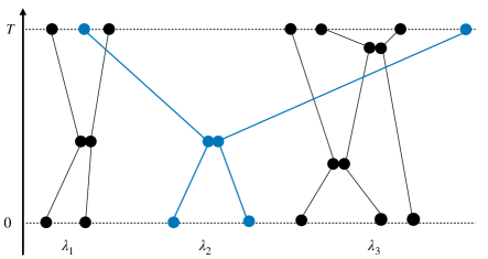
Figure 2: On this figure, three ${\varepsilon}$-cluster paths $\lambda_{1},\lambda_{2},\lambda_{3}$ forming an ${\varepsilon}$-aggregate are depicted (the ${\varepsilon}$-cluster path $\lambda_{2}$ is drawn in blue only for the sake of clarity). The particle dynamics inside each cluster path is not modified by an overlap. Notice that the ${\varepsilon}$-cluster paths $\lambda_{2},\lambda_{3}$ overlap three times, this will be interpreted as a multiple edge in the generalized dynamical interaction graph introduced in Section III.

Within the previous framework, the cluster expansion theory (see e.g. ueltschi2003cluster ; poghosyan2009abstract ) leads to the following result.

Proposition II.6

There exists a time $T>0$ and a constant $C$ depending only on the initial data $f^{0}$ and on the constants $c_{1},c_{2}$ appearing in (17) such that uniformly in ${\varepsilon}$ small enough and for $k\geq 1$

$$\int d|\boldsymbol{\nu}_{{\varepsilon},T}^{(H)}|(\lambda_{1})\dots d|\boldsymbol{\nu}_{{\varepsilon},T}^{(H)}|(\lambda_{k})\;|\varphi_{\varepsilon}(\lambda_{1},\dots,\lambda_{k})|\leq\mu_{\varepsilon}\;k!\;C^{k}\big{(}T+{\varepsilon}\big{)}^{k-1}$$ (32)

and the cluster expansion of the modified partition function converges

$$\log\mathcal{Z}^{\varepsilon}_{T}(e^{H})=\sum_{k\geq 1}\frac{1}{k!}\int d\boldsymbol{\nu}_{{\varepsilon},T}^{(H)}(\lambda_{1})\dots d\boldsymbol{\nu}_{{\varepsilon},T}^{(H)}(\lambda_{k})\;\varphi_{\varepsilon}(\lambda_{1},\dots,\lambda_{k})\,.$$ (33)

Remark II.7

The time $T>0$ for the convergence of the cluster expansion is of the same order as the convergence time $T_{L}$ to the Boltzmann equation in Theorem I.1. In both cases, it is a fraction of the mean collision time between two particles. Indeed the requirement that the gas of ${\varepsilon}$-cluster paths is dilute means that the ${\varepsilon}$-cluster path sizes have to remain small. A crude analogy can be made with an Erdős-Renyi graph built by choosing randomly edges among $N$ points with probability $T/N$. For $T<1$, this procedure leads with high probability to a collection of small graphs which corresponds to the dilute phase we have in mind for the hard sphere dynamics. Instead, as soon as $T>1$, a macroscopic connected graph appears. We will make this analogy more precise in Section IV.2 when analysing the dynamical clustering process. We refer to Gabrielov_Keilis-Borok_Keilis-Borok_Zaliapin ; McFadden_Bouchard ; Patterson_Simonella_Wagner1 ; Patterson_Simonella_Wagner2 ; heydecker2019bilinear for previous works on this dynamical phase transition in the case of particle dynamics. Reaching longer time asymptotics requires therefore new ideas and techniques. For this reason, we have made no attempt to optimise the time convergence $T>0$ in Proposition II.6.

Proof of Proposition II.6.

Assuming the validity of (32), the cluster expansion (33) follows from ueltschi2003cluster . We sketch the proof of (33) below for the sake of completness. Expanding the exclusion with (30) in (29), we get

$$\mathcal{Z}^{\varepsilon}_{T}(e^{H}) =1+\sum_{k\geq 1}\frac{1}{k!}\int d\boldsymbol{\nu}_{{\varepsilon},T}^{(H)}(\lambda_{1})\dots d\boldsymbol{\nu}_{{\varepsilon},T}^{(H)}(\lambda_{k})\;\sum_{\mathcal{G}\in\boldsymbol{\mathcal{G}}_{k}}\prod_{\{j,j^{\prime}\}\in E(\mathcal{G})}\big{(}-{\textbf{1}}_{\lambda_{j}\sim_{\varepsilon}\lambda_{j^{\prime}}}\big{)}\,.$$

Any graph $\mathcal{G}\in\boldsymbol{\mathcal{G}}_{k}$ can be decomposed into connected graphs $\mathcal{G}=\{\mathcal{G}_{1},\dots,\mathcal{G}_{n}\}$ with $|\mathcal{G}_{\ell}|=m_{\ell}$ and $m_{1}+\dots+m_{n}=k$. To do this, we partition $\{1,\dots,k\}$ into $n$ sets and then enumerate the graphs on each set

$$\mathcal{Z}^{\varepsilon}_{T}(e^{H}) =1+\sum_{k=1}^{\infty}\frac{1}{k!}\sum_{n=1}^{k}\frac{1}{n!}\sum_{m_{1},\dots,m_{n}\geq 1\atop m_{1}+\dots+m_{n}=k}\frac{k!}{m_{1}!\dots m_{n}!}\prod_{\ell=1}^{n}\left(\int d\boldsymbol{\nu}_{{\varepsilon},T}^{(H)}(\lambda_{1})\dots d\boldsymbol{\nu}_{{\varepsilon},T}^{(H)}(\lambda_{m_{\ell}})\sum_{\mathcal{G}_{\ell}\in\boldsymbol{\mathcal{C}}_{m_{\ell}}}\prod_{\{j,j^{\prime}\}\in E(\mathcal{G}_{\ell})}\big{(}-{\textbf{1}}_{\lambda_{j}\sim_{\varepsilon}\lambda_{j^{\prime}}}\big{)}\right),$$

where as previously $\frac{k!}{m_{1}!\dots m_{n}!}$ is the number of partitions of $\{1,\dots,k\}$ into $n$ ordered components of cardinalities $m_{1},\dots,m_{n}$ and $\frac{1}{n!}$ removes the multiple counting due to the ordering. Using the definition (31) of ${\varphi}_{\varepsilon}$, we get

$$\mathcal{Z}^{\varepsilon}_{T}(e^{H})=1+\sum_{k=1}^{\infty}\sum_{n=1}^{\infty}1_{n\leq k}\,\frac{1}{n!}\sum_{m_{1},\dots,m_{n}\geq 1\atop m_{1}+\dots+m_{n}=k}\prod_{\ell=1}^{n}\left(\;\frac{1}{m_{\ell}!}\int d\boldsymbol{\nu}_{{\varepsilon},T}^{(H)}(\lambda_{1})\dots d\boldsymbol{\nu}_{{\varepsilon},T}^{(H)}(\lambda_{m_{\ell}})\,\varphi_{\varepsilon}(\lambda_{1},\dots,\lambda_{m_{\ell}})\right).$$

Choosing $T$ small enough, the sums are absolutely convergent thanks to (32) so that they can be swapped

$$\mathcal{Z}^{\varepsilon}_{T}(e^{H}) =1+\sum_{n=1}^{\infty}\frac{1}{n!}\sum_{m_{1},\dots,m_{n}\geq 1}\prod_{\ell=1}^{n}\left(\;\frac{1}{m_{\ell}!}\int d\boldsymbol{\nu}_{{\varepsilon},T}^{(H)}(\lambda_{1})\dots d\boldsymbol{\nu}_{{\varepsilon},T}^{(H)}(\lambda_{m_{\ell}})\,\varphi_{\varepsilon}(\lambda_{1},\dots,\lambda_{m_{\ell}})\right)$$

$$=1+\sum_{n=1}^{\infty}\frac{1}{n!}\left(\sum_{m\geq 1}\;\frac{1}{m!}\int d\boldsymbol{\nu}_{{\varepsilon},T}^{(H)}(\lambda_{1})\dots d\boldsymbol{\nu}_{{\varepsilon},T}^{(H)}(\lambda_{m})\,\varphi_{\varepsilon}(\lambda_{1},\dots,\lambda_{m})\right)^{n}.$$

This is the expansion of the exponential which can be inverted to recover (33).

We turn now to the derivation of the estimate (32) which relies on the specific structure of the microscopic dynamics and more precisely on the geometry of the trajectories in $[0,T]$. We will use the geometric estimates devised in BGSS2 (see also BGSS3 ).

Case $k=1$. We first consider a single ${\varepsilon}$-cluster path $\lambda$ and prove the existence of a time $T_{1}>0$ and of a constant $c_{0}$ such that for $T\leq T_{1}$

$$\int d|\boldsymbol{\nu}_{{\varepsilon},T}^{(H)}|(\lambda)\;e^{\frac{10}{\beta}|\lambda|}\leq c_{0}\mu_{\varepsilon}\,,$$ (34)

where an additional term $e^{\frac{10}{\beta}|\lambda|}$ was added to inequality (32) for later purposes.

Using the definition (27) of $\boldsymbol{\nu}_{{\varepsilon},T}^{(H)}$ and summing over the size $n$ of the cluster path, one has

$$\int d|\boldsymbol{\nu}_{{\varepsilon},T}^{(H)}|(\lambda)e^{\frac{10}{\beta}|\lambda|}=\sum_{n\geq 1}\frac{\mu_{\varepsilon}^{n}}{n\,!}\int e^{\frac{10}{\beta}n}\Big{|}\exp\big{(}H(\lambda)\big{)}\Big{|}\,\left(\prod_{i=1}^{n}f^{0}(z_{i})\,\right)\;{\textbf{1}}_{\lambda~{}\hbox{\scriptsize${\varepsilon}$-cluster path of size}~{}n}\;dZ_{n}\,.$$ (35)

Thanks to assumption (5) on the initial distribution $f^{0}$ and assumption (17) on $H$, we have the following upper bound, for some constant $C^{\prime}_{0}$ depending on $C_{0}$ and $\beta$

$$\Big{|}\exp\big{(}H(\lambda)\big{)}\Big{|}{\textbf{1}}_{|\lambda|=n}\,e^{\frac{10}{\beta}n}\,\prod_{i=1}^{n}f^{0}(z_{i})\leq\Big{(}C^{\prime}_{0}e^{c_{1}+\frac{10}{\beta}}\Big{)}^{n}\;\mathcal{M}_{3\beta/4}^{\otimes n}(V_{n})\,.$$ (36)

Plugging (36) into (35), we see that it is enough to show that there is $C>0$ such that uniformly in $n\geq 2$

$$\int\mathcal{M}_{\beta/4}^{\otimes n}(V_{n})\;{\textbf{1}}_{\lambda\hbox{ \scriptsize${\varepsilon}$-cluster path of size}~{}n}\;dZ_{n}\;\leq n!\frac{C^{n}\,T^{n-1}}{\mu_{\varepsilon}^{n-1}}\;,$$ (37)

and then to choose $T_{1}>0$ small enough to obtain (34) after summation over $n$. Note that only part of the Gaussian weight $\mathcal{M}_{3\beta/4}^{\otimes n}$ in (36) has been used in the above estimate, as we shall need an additional exponential decay later on when dealing with the case $k\geq 2$.

Let us now prove (37). The constraint that $\lambda$ is an ${\varepsilon}$-cluster path of size $n$ imposes that all the particles interact dynamically during the time interval $[0,T]$. We are going to record these collisions in an ordered tree $\mathcal{T}_{\prec}=\{q_{i},\bar{q}_{i}\}_{1\leq i\leq n-1}$ (see Figure 3). There can be more than $n-1$ collisions in the dynamics, but in order to retain a minimal structure and to end up with a tree $\mathcal{T}_{\prec}$, the collisions creating a cycle in the graph are not recorded. The collisions kept in the tree $\mathcal{T}_{\prec}$ will be called clustering collisions : the first collision occurs between particles $q_{1}$ and $\bar{q}_{1}$ at time $\tau_{1}\in[0,T]$, and the last collision is between $q_{n-1}$ and $\bar{q}_{n-1}$ at time $\tau_{n-1}\in(\tau_{n-2},T)$. In this way, an ordered graph recording the dynamical interactions is built by following the flow of the hard sphere dynamics in $[0,T]$. At intermediate times, the graph is made of several connected components, and becomes completely connected at time $\tau_{n-1}$.

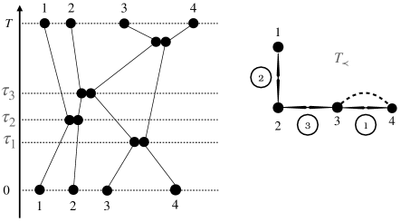
Figure 3: A single cluster path with 4 particles ($n=4$) is depicted on the left and the corresponding collision tree $\mathcal{T}_{\prec}$ is represented on the right. The edges of the tree $\mathcal{T}_{\prec}$ are ordered (circled numbers) according to the order of the collisions in the cluster path $\tau_{1}<\tau_{2}<\tau_{3}\leq T$. Recollisions may occur in the cluster path (as between particles $3$ and $4$ on the picture), but the corresponding (dashed) edge does not belong to $\mathcal{T}_{\prec}$. The collisions associated with the graph edges are called clustering collisions.

The set of all ordered trees with $n$ vertices is denoted by $\boldsymbol{\mathcal{T}}^{\prec}_{n}$. Thus summing over all the trees leads to

$${\textbf{1}}_{\lambda~{}\hbox{\scriptsize${\varepsilon}$-cluster path of size}~{}n}=\sum_{\mathcal{T}_{\prec}\in\boldsymbol{\mathcal{T}}^{\prec}_{n}}{\textbf{1}}_{\{Z_{n}\in\mathcal{R}_{\mathcal{T}_{\prec}}\}}\,,$$ (38)

where $\mathcal{R}_{\mathcal{T}_{\prec}}$ is the set of initial configurations $Z_{n}$ with trajectories compatible with the ordered tree $\mathcal{T}_{\prec}$. By construction for fixed ${\varepsilon}>0$ and for any given $Z_{n}$ coding an ${\varepsilon}$-cluster path, only one term is non zero in the above sum.

For an admissible tree $\mathcal{T}_{\prec}$, the relative positions, at the initial time, of the $i^{\text{th}}$ colliding particles are denoted by

$$\hat{x}_{i}:=x_{q_{i}}-x_{\bar{q}_{i}}\,.$$ (39)

Given the relative positions $(\hat{x}_{j})_{j<i}$ and the velocities $V_{n}$, we consider a forward flow with clustering collisions at times $\tau_{1}<\dots<\tau_{i-1}<T$. By construction, $q_{i}$ and $\bar{q}_{i}$ do not belong to the same connected component in the graph $G_{i-1}$ defined as the graph with edges $\{q_{j},\bar{q}_{j}\}_{1\leq j\leq i-1}$. We shall denote by $\mathcal{C}_{q_{i}}$ and by $\mathcal{C}_{\bar{q}_{i}}$ the connected components associated with $q_{i},\bar{q}_{i}$ at time $\tau_{i-1}$. Inside each connected component, the relative positions are fixed by the dynamical constraints, but the whole component can be translated so that a free parameter remains. Therefore by varying $\hat{x}_{i}$ (moving rigidly the connected components $\boldsymbol{\mathcal{C}}_{q_{i}},\boldsymbol{\mathcal{C}}_{\bar{q}_{i}}$), a collision at time $\tau_{i}\in(\tau_{i-1},T)$ between $q_{i}$ and $\bar{q}_{i}$ can be triggered. If the particles $q_{i}$ and $\bar{q}_{i}$ move in straight lines, then the collision at time $\tau_{i}$ imposes a constraint at time $\tau_{i-1}$

$${\varepsilon}=\big{|}{\textbf{x}}^{{\varepsilon}}_{q_{i}}(\tau_{i})-{\textbf{x}}^{{\varepsilon}}_{\bar{q}_{i}}(\tau_{i})\big{|}=\big{|}{\textbf{x}}^{{\varepsilon}}_{q_{i}}(\tau_{i-1})-{\textbf{x}}^{{\varepsilon}}_{\bar{q}_{i}}(\tau_{i-1})-(\tau_{i}-\tau_{i-1})\big{(}\textbf{v}^{\varepsilon}_{q_{i}}(\tau_{i-1}^{+})-\textbf{v}^{\varepsilon}_{\bar{q}_{i}}(\tau_{i-1}^{+})\big{)}\big{|}\,.$$ (40)

This says that the relative position at time $\tau_{i-1}$ has to belong to a tube of direction $\textbf{v}^{\varepsilon}_{q_{i}}(\tau_{i-1}^{+})-\textbf{v}^{\varepsilon}_{\bar{q}_{i}}(\tau_{i-1}^{+})$ with diameter ${\varepsilon}$ and length $|\textbf{v}^{\varepsilon}_{q_{i}}(\tau^{+}_{i-1})-\textbf{v}^{\varepsilon}_{\bar{q}_{i}}(\tau^{+}_{i-1})|\left(T-\tau_{i-1}\right)$ so that the collision occurs before time $T$. Since the trajectories inside each connected components are fixed up to a global translation, this condition can be expressed in terms of the initial relative position : $\hat{x}_{i}\in\mathcal{B}_{\mathcal{T}_{\prec},i}(\hat{x}_{1},\dots,\hat{x}_{i-1},V_{n})$. Thus, the measure of the set $\mathcal{B}_{\mathcal{T}_{\prec},i}$ is bounded from above by (recall $\mu_{\varepsilon}={\varepsilon}^{-(d-1)}$)

$$|\mathcal{B}_{\mathcal{T}_{\prec},i}|\leq\frac{C}{\mu_{\varepsilon}}|\textbf{v}^{\varepsilon}_{q_{i}}(\tau^{+}_{i-1})-\textbf{v}^{\varepsilon}_{\bar{q}_{i}}(\tau^{+}_{i-1})|\;\int^{T}_{\tau_{i-1}}d\tau_{i}\;.$$ (41)

If the particle $q_{i}$ (resp. $\bar{q}_{i}$) has been deflected during $[\tau_{i-1},\tau_{i}[$ (by recollisions with particles in the connected component of $\boldsymbol{\mathcal{C}}_{q_{i}}$ (resp. $\boldsymbol{\mathcal{C}}_{\bar{q}_{i}}$)) then one has to decompose the trajectories into a union of tubes (as in Chapter 8 of BGSS2 ) and an estimate as (41) can be recovered. Summing over all the possible pairs of particles and using the fact that collisions preserve the kinetic energy, we get after a Cauchy-Schwarz inequality

$$\sum_{q_{i},\bar{q}_{i}}|\mathcal{B}_{\mathcal{T}_{\prec},i}|\leq\frac{C}{\mu_{\varepsilon}}\left({\mathcal{E}}_{\lambda}+n\right)n\;\int^{T}_{\tau_{i-1}}d\tau_{i}\;,$$ (42)

where ${\mathcal{E}}_{\lambda}:=V_{n}^{2}/2$ is the total kinetic energy of the particles in the cluster path. Iterating the previous estimates, we get from Fubini’s theorem

$$\sum_{\mathcal{T}_{\prec}\in\boldsymbol{\mathcal{T}}^{\prec}_{n}}\int d\hat{X}_{n-1}\prod_{i=1}^{n-1}{\textbf{1}}_{\mathcal{B}_{\mathcal{T}_{\prec},i}} \leq\sum_{\mathcal{T}_{\prec}\in\boldsymbol{\mathcal{T}}^{\prec}_{n}}\int d\hat{x}_{1}{\textbf{1}}_{\mathcal{B}_{\mathcal{T}_{\prec},1}}\int d\hat{x}_{2}\,\dots\int d\hat{x}_{n-1}{\textbf{1}}_{\mathcal{B}_{\mathcal{T}_{\prec},n-1}}$$

$$\leq\left(\frac{C}{\mu_{\varepsilon}}\right)^{n-1}\left({\mathcal{E}}_{\lambda}+n\right)^{n-1}n^{n-1}\int_{0}^{T}d\tau_{1}\,\dots\int_{\tau_{n-2}}^{T}d\tau_{n-1}\leq\left(\frac{C}{\mu_{\varepsilon}}\right)^{n-1}\left({\mathcal{E}}_{\lambda}+n\right)^{n-1}n^{n-1}\frac{T^{n-1}}{(n-1)!},$$ (43)

where the last inequality follows by integrating the ordered times. Furthermore, for any $K,N$

$$\sup_{V\in\mathbb{R}^{dN}}\Big{\{}\exp\big{(}-\frac{\beta}{4}|V|^{2}\big{)}\;(|V|^{2}+K)^{N}\Big{\}}\leq C_{\beta}^{N}e^{\frac{\beta}{4}K}\;N^{N}.$$ (44)

Using the Gaussian integration in (37), we deduce from the previous inequality that the term $\left({\mathcal{E}}_{\lambda}+n\right)^{n}$ leads to another factor of order $n^{n}$ which is (up to a factor $C^{n}$) of the same order as $n!$. Recalling (38), this completes (37) and thus (34).

Remark II.8

Let us call the root of $\lambda$ the position $y:=\displaystyle\frac{1}{n}\sum_{i=1}^{n}x_{i}$ of the center of mass of the particles in $\lambda$ at time 0, where $n=|\lambda|$. The change of variables $X_{n}\mapsto(\hat{X}_{n-1},y)$ has unit Jacobian. Moreover, since the ${\varepsilon}$-cluster path $\lambda$ is invariant by translations, its root is not constrained by the collision conditions.

Case $k>1$. We derive now (32) for a non trivial ${\varepsilon}$-aggregate with $k$ ${\varepsilon}$-cluster paths: let us prove that for $T$ small enough (smaller than $T_{1}$ (see (34)) and independent of $k$)

$$\int d|\boldsymbol{\nu}_{{\varepsilon},T}^{(H)}|(\lambda_{1})\dots d|\boldsymbol{\nu}_{{\varepsilon},T}^{(H)}|(\lambda_{k})\;\varphi_{\varepsilon}(\lambda_{1},\dots,\lambda_{k})\leq\mu_{\varepsilon}\;k!\,C^{k}\,\big{(}T+{\varepsilon}\big{)}^{k-1}.$$

For this, we are going to use the inequality (34) which evaluates the constraints, in each cluster path $\lambda_{\ell}$, on the coordinates of the particles $Z^{(\ell)}_{|\lambda_{\ell}|}$ at time 0. Further dynamical constraints are added by the function $\varphi_{\varepsilon}(\lambda_{1},\dots,\lambda_{k})$ defined in (31). Viewing the overlaps between the ${\varepsilon}$-cluster paths as the edges of a graph with $k$ vertices indexing the ${\varepsilon}$-cluster paths $\lambda_{1},\dots,\lambda_{k}$, then the alternating sums defining $\varphi_{\varepsilon}(\lambda_{1},\dots,\lambda_{k})$ can be bounded from above by the so called tree inequality

$$\big{|}\varphi_{\varepsilon}(\lambda_{1},\dots,\lambda_{k})\big{|}=\Big{|}\sum_{\mathcal{G}\in\boldsymbol{\mathcal{C}}_{k}}\prod_{\{j,j^{\prime}\}\in E(\mathcal{G})}(-{\textbf{1}}_{\lambda_{j}\sim_{\varepsilon}\lambda_{j^{\prime}}})\Big{|}\leq\sum_{\mathcal{T}^{ov}\in\boldsymbol{\mathcal{T}}_{k}}\ \ \prod_{\{j,j^{\prime}\}\in E(\mathcal{T}^{ov})}{\textbf{1}}_{\lambda_{j}\sim_{\varepsilon}\lambda_{j^{\prime}}}\,,$$ (45)

where the sum is restricted to (non-ordered) trees. The tree inequality (45) which allows to control $\varphi_{\varepsilon}$ follows from a standard combinatorial argument (see penrose1967convergence ) which will not be recalled here. Note that in (45), several graphs can be compatible with the same family of ${\varepsilon}$-cluster paths $(\lambda_{1},\dots,\lambda_{k})$ so that several trees $\mathcal{T}^{ov}$ may contribute to the sum.

Since the particle trajectories are unchanged by the overlaps, it is not needed to proceed as for the collisions within the ${\varepsilon}$-cluster paths and to prescribe an order related to the dynamical overlaps on the edges of $\mathcal{T}^{ov}$. Thus, for each $\mathcal{T}^{ov}$, we have more flexibility in choosing the integration variables and we can order the edges following for instance the depth of vertices in the graph (see BGSS2 for details). We then examine successively the $k-1$ overlap constraints imposed on the ${\varepsilon}$-cluster paths. Denote by $\lambda_{p_{i}},\lambda_{\bar{p}_{i}}$ the ${\varepsilon}$-cluster paths involved in the $i^{\text{th}}$ overlap and by $q_{i}$ and $\bar{q}_{i}$ the two overlapping particles. The constraint imposed by the $i^{\text{th}}$ overlap leads to a condition on the relative position of the two cluster paths at the initial time (see (39))

$$\hat{y}_{i}:=y_{p_{i}}-y_{\bar{p}_{i}}\,,$$

recalling the notation for the root introduced in Remark II.8. Indeed, fixing the velocities and the relative positions in each cluster path, one has to evaluate the condition for the set

$$\big{\{}\hat{y}_{i}+(x_{q_{i}}(t)-y_{p_{i}})-(x_{\bar{q}_{i}}(t)-y_{\bar{p}_{i}});\quad t\leq T\big{\}}$$

to intersect a ball of radius ${\varepsilon}$ around the origin. Note that, contrary to the collisions, the overlap may occur at the initial time or dynamically. This condition on $\hat{y}_{i}$ is coded by the set $\mathcal{B}_{\mathcal{T}^{ov},i}$ with measure bounded by

$$|\mathcal{B}_{\mathcal{T}^{ov},i}|\leq C{\varepsilon}^{d}+\frac{C}{\mu_{\varepsilon}}\int_{0}^{T}ds\;|\textbf{v}^{\varepsilon}_{q_{i}}(s)-\textbf{v}^{\varepsilon}_{\bar{q}_{i}}(s)|\,.$$ (46)

We stress the fact that ${\varepsilon}^{d}$ corresponds to the cost of an overlap at time 0 which is much smaller than the cost $\frac{1}{\mu_{\varepsilon}}={\varepsilon}^{d-1}$ of a dynamical overlap. This fact will be used in the Boltzmann-Grad limit to neglect the overlaps occurring at the initial time.

Denoting as previously by $|\lambda|$ the cardinality of an ${\varepsilon}$-cluster path and summing over all the possible particles in the ${\varepsilon}$-cluster paths $\lambda_{p_{i}},\lambda_{\bar{p}_{i}}$, we get by a Cauchy-Schwarz inequality

$$\sum_{q_{i},\bar{q}_{i}}|\mathcal{B}_{\mathcal{T}^{ov},i}| \leq C{\varepsilon}^{d}\;|\lambda_{\bar{p}_{i}}|\;|\lambda_{p_{i}}|+\frac{C}{\mu_{\varepsilon}}\int_{0}^{T}ds\;\left(|\lambda_{p_{i}}|\;\sqrt{|\lambda_{\bar{p}_{i}}|}\sqrt{\mathcal{E}_{\lambda_{\bar{p}_{i}}}}+|\lambda_{\bar{p}_{i}}|\;\sqrt{|\lambda_{p_{i}}|}\sqrt{\mathcal{E}_{\lambda_{p_{i}}}}\right)$$

$$\leq C{\varepsilon}^{d}\;|\lambda_{\bar{p}_{i}}|\;|\lambda_{p_{i}}|+\frac{C}{\mu_{\varepsilon}}T\;\Big{(}\frac{\beta}{4}\mathcal{E}_{\lambda_{\bar{p}_{i}}}+\frac{4}{\beta}|\lambda_{\bar{p}_{i}}|\Big{)}\Big{(}\frac{\beta}{4}\mathcal{E}_{\lambda_{p_{i}}}+\frac{4}{\beta}|\lambda_{p_{i}}|\Big{)}\leq\frac{C}{\mu_{\varepsilon}}(T+{\varepsilon})\;\Big{(}\frac{\beta}{4}\mathcal{E}_{\lambda_{\bar{p}_{i}}}+\frac{4}{\beta}|\lambda_{\bar{p}_{i}}|\Big{)}\Big{(}\frac{\beta}{4}\mathcal{E}_{\lambda_{p_{i}}}+\frac{4}{\beta}|\lambda_{p_{i}}|\Big{)},$$ (47)

where we used in the second inequality that the total kinetic energy $\mathcal{E}_{\lambda}$ of the particles in an ${\varepsilon}$-cluster path $\lambda$ is constant in time. Thus (47) measures the cost of the overlap coded by the edge $\{\lambda_{\bar{p}_{i}},\lambda_{p_{i}}\}$ in the tree $\mathcal{T}^{ov}$.

Let $\mathcal{B}_{\mathcal{T}^{ov}}$ be the set representing all the conditions imposed by the overlaps. Given $\{\mathcal{E}_{\lambda_{1}},\dots,\mathcal{E}_{\lambda_{k}}\}$ the energies of all the ${\varepsilon}$-cluster paths, the measure of $\mathcal{B}_{\mathcal{T}^{ov}}$ with respect to the relative positions $(\hat{y}_{i})_{i\leq k-1}$ of the ${\varepsilon}$-cluster paths is obtained by multiplying the contributions (47) for each edge of the tree $\mathcal{T}^{ov}$

$$|\mathcal{B}_{\mathcal{T}^{ov}}|\leq\left(\frac{C}{\mu_{\varepsilon}}\right)^{k-1}\;(T+{\varepsilon})^{k-1}\;\prod_{i=1}^{k}\Big{(}\frac{\beta}{4}\mathcal{E}_{\lambda_{i}}+\frac{4}{\beta}|\lambda_{i}|\Big{)}^{d_{i}},$$

where $d_{i}$ stands for the degree of the vertex $\lambda_{i}$ in the tree $\mathcal{T}^{ov}$. There are $(k-2)!/\prod_{i}(d_{i}-1)!$ trees of size $k$ with specified vertex degrees (see e.g. Lemma 2.4.1 in BGSS2 ). Thus summing over all the trees $\mathcal{T}^{ov}$, we get

$$\sum_{\mathcal{T}^{ov}\in\boldsymbol{\mathcal{T}}_{k}}|\mathcal{B}_{\mathcal{T}^{ov}}| \leq\left(\frac{C}{\mu_{\varepsilon}}\right)^{k-1}\;(T+{\varepsilon})^{k-1}(k-2)!\sum_{d_{1},\dots d_{k}\atop d_{1}+\dots d_{k}=2k-2}\;\prod_{i=1}^{k}\frac{\Big{(}\frac{\beta}{4}\mathcal{E}_{\lambda_{i}}+\frac{4}{\beta}|\lambda_{i}|\Big{)}^{d_{i}}}{\left(d_{i}-1\right)!}$$

$$\leq\left(\frac{C}{\mu_{\varepsilon}}\right)^{k-1}\;(T+{\varepsilon})^{k-1}(k-2)!\;\prod_{i=1}^{k}\left(\frac{\beta}{4}\mathcal{E}_{\lambda_{i}}+\frac{4}{\beta}|\lambda_{i}|\right)\;\exp\left(\frac{\beta}{4}\mathcal{E}_{\lambda_{i}}+\frac{4}{\beta}|\lambda_{i}|\right),$$

where the constraint on the degrees is released in the last inequality to recover the exponential.

Using the Gaussian weights $\mathcal{M}_{\beta/2}^{\otimes|\lambda_{i}|}$ from the initial measure as well as the inequality (44), we obtain an upper bound for the overlaps of the form

$$\sum_{\mathcal{T}^{ov}\in\boldsymbol{\mathcal{T}}_{k}}|\mathcal{B}_{\mathcal{T}^{ov}}|\;\prod_{i=1}^{k}\mathcal{M}_{\beta/2}^{\otimes|\lambda_{i}|}(Z_{|\lambda_{i}|})\leq\frac{C^{k}}{\mu_{\varepsilon}^{k-1}}\,k!\,(T+{\varepsilon})^{k-1}\prod_{i=1}^{k}e^{\frac{10}{\beta}|\lambda_{i}|}.$$ (48)

Once the dynamical constraint on the overlaps has been taken into account, the contributions of the cluster paths are independent and can be estimated by (34) for $T$ small enough (independently of $k$)

$$\prod_{i=1}^{k}\int d|\boldsymbol{\nu}_{{\varepsilon},T}^{(H)}|(\lambda_{i})\,e^{\frac{10}{\beta}|\lambda_{i}|}\;\leq c_{0}^{k}\mu_{\varepsilon}^{k}.$$ (49)

Combining (45), (48) and (49), we deduce that

$$\int d|\boldsymbol{\nu}_{{\varepsilon},T}^{(H)}|(\lambda_{1})\;\dots\;d|\boldsymbol{\nu}_{{\varepsilon},T}^{(H)}|(\lambda_{k})\;\varphi_{\varepsilon}(\lambda_{1},\dots,\lambda_{k})\leq\mu_{\varepsilon}\;k!\;C^{k}\,(T+{\varepsilon})^{k-1}.$$ (50)

This completes the proof of (32) for a value of $T>0$ small enough so that (34) holds. Proposition II.6 is proved.

II.3 Measure concentration properties

We are going to deduce now some consequences of the cluster expansion for fixed (but large) $\mu_{\varepsilon}$. The exponential moments $\Lambda^{\varepsilon}_{T}$ introduced in (21) encode the statistics of the cluster paths. Choosing $T>0$ as in Proposition II.6, we know that the functional $\Lambda^{\varepsilon}_{T}(e^{uH})$ is analytic with respect to $u$ and its derivatives at $u=0$ are uniformly controlled in $\mu_{\varepsilon}$. This is an important property as the derivatives of the functional are related to physical quantities. Indeed considering for instance the first derivative at 0 of $u\in\mathbb{R}\mapsto\Lambda^{\varepsilon}_{T}(e^{u\,H})$, we recover the expectation of the empirical measure (using the notation of (20))

$$\mathbb{E}_{\varepsilon}\left[\Pi^{\varepsilon}_{[0,T]}(H)\right]=\partial_{u}\,\Lambda^{\varepsilon}_{T}(e^{u\,H})\Big{|}_{u=0}=\frac{1}{\mu_{\varepsilon}}\sum_{k\geq 1}\frac{1}{k!}\int d\boldsymbol{\nu}_{{\varepsilon},T}^{(0)}(\lambda_{1})\dots d\boldsymbol{\nu}_{{\varepsilon},T}^{(0)}(\lambda_{k})\;\varphi_{\varepsilon}(\lambda_{1},\dots,\lambda_{k})\left(\sum_{\ell=1}^{k}H\big{(}\lambda_{\ell}\big{)}\right).$$ (51)

Using the symmetry between the clusters, we recover the distribution of a typical ${\varepsilon}$-cluster path

$$\mathbb{E}_{\varepsilon}\left[\Pi^{\varepsilon}_{[0,T]}(H)\right]=\int d\boldsymbol{\Upsilon}_{{\varepsilon},T}(\lambda_{1})H(\lambda_{1}),$$ (52)

where

$$d\boldsymbol{\Upsilon}_{{\varepsilon},T}(\lambda_{1})=\frac{1}{\mu_{\varepsilon}}\left(d\boldsymbol{\nu}_{{\varepsilon},T}^{(0)}(\lambda_{1})+\sum_{k\geq 2}\frac{1}{(k-1)!}d\boldsymbol{\nu}_{{\varepsilon},T}^{(0)}(\lambda_{1})\int d\boldsymbol{\nu}_{{\varepsilon},T}^{(0)}(\lambda_{2})\dots d\boldsymbol{\nu}_{{\varepsilon},T}^{(0)}(\lambda_{k})\;\varphi_{\varepsilon}(\lambda_{1},\dots,\lambda_{k})\right).$$ (53)

Taking twice the derivative leads to the variance

$$\mathbb{E}_{\varepsilon}\left[\left(\Pi^{\varepsilon}_{[0,T]}(H)-\mathbb{E}_{\varepsilon}\left[\Pi^{\varepsilon}_{[0,T]}(H)\right]\right)^{2}\right]=\mathbb{E}_{\varepsilon}\left[\Pi^{\varepsilon}_{[0,T]}(H)^{2}\right]-\mathbb{E}_{\varepsilon}\left[\Pi^{\varepsilon}_{[0,T]}(H)\right]^{2}=\frac{1}{\mu_{\varepsilon}}\partial^{2}_{u}\,\Lambda^{\varepsilon}_{T}(e^{u\,H})\Big{|}_{u=0}.$$ (54)

As a corollary of Proposition II.6, the second derivative is uniformly bounded with respect to $\mu_{\varepsilon}$

$$\partial^{2}_{u}\,\Lambda^{\varepsilon}_{T}(e^{u\,H})\Big{|}_{u=0} =\frac{1}{\mu_{\varepsilon}}\sum_{k\geq 1}\frac{1}{k!}\int d\boldsymbol{\nu}_{{\varepsilon},T}^{(0)}(\lambda_{1})\dots d\boldsymbol{\nu}_{{\varepsilon},T}^{(0)}(\lambda_{k})\;\varphi_{\varepsilon}(\lambda_{1},\dots,\lambda_{k})\left(\sum_{\ell=1}^{k}H\big{(}\lambda_{\ell}\big{)}\right)^{2}$$ (55)

$$\leq\frac{1}{\mu_{\varepsilon}}\sum_{k\geq 1}\frac{1}{k!}\int d|\boldsymbol{\nu}_{{\varepsilon},T}^{(0)}|(\lambda_{1})\dots d|\boldsymbol{\nu}_{{\varepsilon},T}^{(0)}|(\lambda_{k})\;\varphi_{\varepsilon}(\lambda_{1},\dots,\lambda_{k})\left(\sum_{\ell=1}^{k}c_{1}|\lambda_{\ell}|+c_{2}\mathcal{E}_{\lambda_{\ell}}\right)^{2}=O(1)\,,$$

for test functions $H$ satisfying (17).

This implies that the covariance vanishes in the Boltzmann-Grad limit so that the empirical measure concentrates to its mean

$$\mathbb{E}_{\varepsilon}\left[\left(\Pi^{\varepsilon}_{[0,T]}(H)-\mathbb{E}_{\varepsilon}\left[\Pi^{\varepsilon}_{[0,T]}(H)\right]\right)^{2}\right]=O\left(\frac{1}{\mu_{\varepsilon}}\right).$$ (56)

Applying this result to functions $H(\lambda)=\displaystyle\sum_{i=1}^{|\lambda|}h\big{(}{\textbf{z}}_{i}([0,T])\big{)}$ as in (19), we deduce in particular the concentration of the empirical measure (13) to its mean

$$\mathbb{E}_{\varepsilon}\left[\left(\pi^{\varepsilon}_{[0,T]}(h)-\mathbb{E}_{\varepsilon}\left[\pi^{\varepsilon}_{[0,T]}(h)\right]\right)^{2}\right]=O\left(\frac{\|h\|_{\infty}^{2}}{\mu_{\varepsilon}}\right).$$ (57)

By taking further derivatives, one can recover all the cumulants studied in BGSS2 and show that the $L^{1}$-norm of the (unrescaled) cumulant of order $n$ decays as $O\left(\mu_{\varepsilon}^{1-n}\right)$. This result was already obtained in BGSS2 (see Theorem 4 therein). Notice however that the series expansion for $\widetilde{\Lambda}^{\varepsilon}_{T}(e^{h})$ is derived in BGSS2 by applying a cluster expansion on the Duhamel representation of the correlation functions and the terms of the series are described by pseudo-trajectories instead of physical trajectories (see Eq.s (4.4.7) and (4.4.1) in BGSS2 ).

III The Boltzmann-Grad limit

The series expansion (33) in Proposition II.6 provides a representation of the partition function $\log\mathcal{Z}^{\varepsilon}_{T}(e^{H})$ in terms of generalized dynamical interactions (collisions and overlaps) of microscopic trajectories. The estimates derived in the previous section hold uniformly with respect to $\mu_{\varepsilon}$ (large enough). In this section, we are going focus on the kinetic limit $\mu_{\varepsilon}\to\infty$. We are going to show that the structure of these interactions simplifies in that limit, providing a simpler (but singular) expansion.

III.1 Discarding recollisions and non minimal overlaps

We first consider the dynamical interactions (collisions) within an ${\varepsilon}$-cluster path $\lambda$ and show that, in the Boltzmann-Grad limit, the only relevant trajectories have exactly $|\lambda|-1$ collisions. Recall that in this ${\varepsilon}$-cluster path $\lambda$, all the particles interact dynamically in the sense of Definition II.1. All these interactions can be recorded in a dynamical interaction graph $\mathcal{G}$ with $|\lambda|$ vertices labelled by the particles and edges corresponding to a collision between two particles. By definition of the ${\varepsilon}$-cluster path $\lambda$, the graph $\mathcal{G}$ is connected and it may have cycles or multiple edges (see the black cluster path in Figure 4).

These cycles correspond to recollisions in the hard sphere dynamics starting from the initial configuration $Z_{|\lambda|}$. We stress the fact that this notion of recollision slightly differs from the interpretation of recollisions used in the Duhamel representation Cercignani_Illner_Pulvirenti ; Spohn_fluctuations ; Pulvirenti_Simonella ; BGSS2 .

In the Boltzmann-Grad limit, the only relevant graphs will be trees, i.e. minimally connected graphs. To discuss the convergence in this limit, it is then useful to introduce a truncated measure which (with respect to (27)) forbids the recollisions. We say that an ${\varepsilon}$-cluster path $\lambda$ is minimal, or (for brevity) a min ${\varepsilon}$-cluster path, if its dynamical interaction graph is a tree. We define the following truncated integration measure :

$$d\boldsymbol{\nu}_{{\varepsilon},T}^{(H),\hbox{\rm\scriptsize min}}(\lambda):=\frac{\mu_{\varepsilon}^{|\lambda|}}{|\lambda|\,!}\,{\textbf{1}}_{{\lambda}\text{ \scriptsize min ${\varepsilon}$-cluster path on $[0,T]$ }}\,F^{(H)}(\lambda)\;dZ_{|\lambda|}\;.$$ (58)

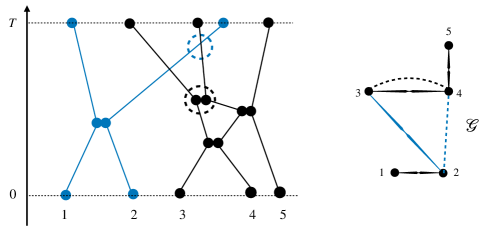
Figure 4: On the left, two overlapping ${\varepsilon}$-cluster paths are represented with different colors. The dynamical interaction graph is depicted on the right with black edges for the collisions and blue edges for the overlaps. The minimal dynamical graph is shown in solid lines, instead the recollisions and multiple overlaps are represented by dashed edges.

In the proof of Proposition II.6, Estimate (34), recalled below,

$$\int d|\boldsymbol{\nu}_{{\varepsilon},T}^{(H)}|(\lambda)\,e^{\frac{10}{\beta}|\lambda|}\leq C_{0}\mu_{\varepsilon}$$

was derived by showing that the collisions between particles in an ${\varepsilon}$-cluster path can be indexed by a tree. This tree records the minimal amount of dynamical constraints and the recollisions add more constraints which can be controlled by the geometric estimates derived in BGSS3 (see Eq (5.12) and Appendix B), leading to

$$\Big{|}\int d\boldsymbol{\nu}_{{\varepsilon},T}^{(H),\hbox{\rm\scriptsize min}}(\lambda)\,e^{\frac{10}{\beta}|\lambda|}-\int d\boldsymbol{\nu}_{{\varepsilon},T}^{(H)}(\lambda)\,e^{\frac{10}{\beta}|\lambda|}\Big{|}\leq C\,\mu_{\varepsilon}\;{\varepsilon}^{\alpha}$$ (59)

for $\alpha<1$, in dimension $d\geq 3$ and for $T$ small enough as in Proposition II.6. In dimension 2, similar geometric arguments provide the same bound.

The second type of dynamical interactions are the overlaps, introduced in Definition II.4. We consider now $k$ overlapping cluster paths $\lambda_{1},\dots,\lambda_{k}$. The combinatorial factor $\varphi_{\varepsilon}(\lambda_{1},\dots,\lambda_{k})$ has been estimated in (45), recalled below, as an upper bound on trees with edges between two overlapping ${\varepsilon}$-cluster paths

$$\big{|}\varphi_{\varepsilon}(\lambda_{1},\dots,\lambda_{k})\big{|}\leq\sum_{\mathcal{T}^{ov}\in\boldsymbol{\mathcal{T}}_{k}}\prod_{\{j,j^{\prime}\}\in E(\mathcal{T}^{ov})}{\textbf{1}}_{\lambda_{j}\sim_{\varepsilon}\lambda_{j^{\prime}}}.$$

If the graph recording all the overlaps of $(\lambda_{1},\dots,\lambda_{k})$ has cycles, then several trees $\mathcal{T}^{ov}$ will contribute to the sum above. But we can actually show that cycles (see Figure 4) can be neglected in the limit and that typically the constraint $\varphi_{\varepsilon}(\lambda_{1},\dots,\lambda_{k})$ is compatible with a single tree. Furthermore, as noted in the comment after (46), the overlaps occurring initially have a much smaller cost than the dynamical overlaps. Thus they can also be neglected in the Boltzmann-Grad limit.

This means that also in the case of overlaps, the only relevant dynamical interaction graphs are trees. When $\{\lambda_{1},\dots,\lambda_{k}\}$ has such a minimal interaction graph, we say that it is a minimal ${\varepsilon}$-aggregate. By definition, the aggregate function $\varphi_{\varepsilon}$ restricted to minimal ${\varepsilon}$-aggregates takes the value $(-1)^{k-1}$ and is defined by

$$\varphi_{\varepsilon}^{\hbox{\scriptsize min}}(\lambda_{1},\dots,\lambda_{k}):=(-1)^{k-1}1_{\{\lambda_{1},\dots,\lambda_{k}\}\hbox{\scriptsize min ${\varepsilon}$-aggregate}}\,.$$ (60)

Combining the proof of Proposition II.6 and the geometric estimates derived in BGSS3 , one can show that the overlaps forming cycles do not contribute in the Boltzmann-Grad limit. As the recollisions can also be neglected thanks to (59), we finally obtain that the minimally connected graphs provide the leading contribution to the cluster expansion series.

Proposition III.1

Let $T>0$ be the convergence time obtained in Proposition II.6. There are constants $C,\alpha\in(0,1)$ such that uniformly in ${\varepsilon}$ small enough and for $k\geq 1$

$$\left|\int d\boldsymbol{\nu}_{{\varepsilon},T}^{(H),\hbox{\rm\scriptsize min}}(\lambda_{1})\dots d\boldsymbol{\nu}_{{\varepsilon},T}^{(H),\hbox{\rm\scriptsize min}}(\lambda_{k})\;\varphi_{\varepsilon}^{\hbox{ \rm\scriptsize min}}(\lambda_{1},\dots,\lambda_{k})-\int d\boldsymbol{\nu}_{{\varepsilon},T}^{(H)}(\lambda_{1})\dots d\boldsymbol{\nu}_{{\varepsilon},T}^{(H)}(\lambda_{k})\;\varphi_{\varepsilon}(\lambda_{1},\dots,\lambda_{k})\right|\leq\mu_{\varepsilon}\;{\varepsilon}^{\alpha}\;k!\;C^{k}(T+{\varepsilon})^{k-1}.$$ (61)

As a consequence,

$$\left|\log\mathcal{Z}_{T}^{\varepsilon}(e^{H})-\sum_{k\geq 1}\frac{1}{k!}\int d\boldsymbol{\nu}_{{\varepsilon},T}^{(H),\hbox{\rm\scriptsize min}}(\lambda_{1})\dots d\boldsymbol{\nu}_{{\varepsilon},T}^{(H),\hbox{\rm\scriptsize min}}(\lambda_{k})\;\varphi_{\varepsilon}^{\hbox{ \rm\scriptsize min}}(\lambda_{1},\dots,\lambda_{k})\right|\leq C\,\mu_{\varepsilon}\;{\varepsilon}^{\alpha}.$$ (62)

Remark III.2

The term $\displaystyle\int d\boldsymbol{\nu}_{{\varepsilon},T}^{(H),\hbox{\rm\scriptsize min}}(\lambda_{1})\dots d\boldsymbol{\nu}_{{\varepsilon},T}^{(H),\hbox{\rm\scriptsize min}}(\lambda_{k})\;\varphi_{\varepsilon}^{\hbox{ \rm\scriptsize min}}(\lambda_{1},\dots,\lambda_{k})$ in (61) corresponds to minimally connected dynamical graphs, and can be rewritten differently by treating collisions and overlaps in a more symmetric way.

Given $\{\lambda_{1},\dots,\lambda_{k}\}$ a set of overlapping ${\varepsilon}$-cluster paths, the corresponding particle configuration will be linked by $|\lambda_{\ell}|-1$ collisions in each cluster path $\lambda_{\ell}$ and $k-1$ overlaps between cluster paths. In particular, if $n$ stands for the total number of particles in $\{\lambda_{1},\dots,\lambda_{k}\}$, we say that there are $n-1=\sum_{\ell=1}^{k}(|\lambda_{\ell}|-1)+k-1$ “clustering conditions” (generalizing the clustering collisions introduced at the level of (38)).

Ordering all these clustering conditions according to the forward flow, we index them by a single signed ordered tree $\overline{\mathcal{T}_{\prec}}$ such that the $n$ particles form the vertices and each edge $e$ has a sign $s_{e}=+1$ if it records a collision or $s_{e}=-1$ if it records an overlap. Thus instead of decomposing the particles into overlapping ${\varepsilon}$-cluster paths, one can choose globally a set of $n$ particles whose trajectories are denoted by ${\textbf{Z}}^{\varepsilon}_{n}:={\textbf{Z}}^{\varepsilon}_{n}([0,T])$ and signed ordered trees $\overline{\mathcal{T}_{\prec}}$ coding the clustering conditions. By Fubini’s theorem, we deduce that

$$\sum_{k\geq 1}\frac{1}{k!}\int d\boldsymbol{\nu}_{{\varepsilon},T}^{(H),\hbox{\rm\scriptsize min}}(\lambda_{1})\dots d\boldsymbol{\nu}_{{\varepsilon},T}^{(H),\hbox{\rm\scriptsize min}}(\lambda_{k})\;\varphi_{\varepsilon}^{\hbox{ \rm\scriptsize min}}(\lambda_{1},\dots,\lambda_{k})=\sum_{n=1}^{\infty}\frac{\mu_{\varepsilon}^{n}}{n!}\sum_{\overline{\mathcal{T}_{\prec}}\in\boldsymbol{\mathcal{T}}_{n}^{\prec,\pm}}\;\Big{(}\prod_{e\in\overline{\mathcal{T}_{\prec}}}s_{e}\Big{)}\;\int dZ_{n}\;F^{(H)}({\textbf{Z}}^{\varepsilon}_{n})\;{\textbf{1}}_{{\textbf{Z}}^{\varepsilon}_{n}\ \hbox{\rm\scriptsize compatible with }\overline{\mathcal{T}_{\prec}}}$$

where $\boldsymbol{\mathcal{T}}_{n}^{\prec,\pm}$ is the set of signed ordered trees with $n$ vertices indexing the particle trajectories with initial data $Z_{n}$.

III.2 Asymptotics of the partition function

We are going to use Proposition III.1 to compute the asymptotics of the partition function when $\mu_{\varepsilon}$ tends to infinity. In the Boltzmann-Grad limit, the particle trajectories in the series expansion (33) become singular, but a limiting structure can be identified using a suitable parametrization of the ${\varepsilon}$-cluster paths.

We first consider the dynamical interactions within a min ${\varepsilon}$-cluster path $\lambda$ of size $n$, and assume that the collisions are prescribed by the ordered tree $\mathcal{T}_{\prec}$. For fixed ${\varepsilon}>0$, the collision condition associated with the edge $e=\{i,j\}$ takes the form

$$\omega_{e}:=\frac{{\textbf{x}}_{i}^{\varepsilon}(\tau_{e})-{\textbf{x}}_{j}^{\varepsilon}(\tau_{e})}{{\varepsilon}}\in{\mathbb{S}}^{d-1}\,,$$ (63)

denoting by $\tau_{e}$ the collision time. Recall that before the collision, the particles $i,j$ are connected to two distinct components of the dynamical graph which can move rigidly with the positions of $i$ and $j$ at time zero. We know that the coordinates $\big{(}{\textbf{x}}_{i}^{\varepsilon}(\tau_{e}^{-})-x_{i},{\textbf{v}}_{i}^{\varepsilon}(\tau_{e}^{-})\big{)}$ and $\big{(}{\textbf{x}}_{j}^{\varepsilon}(\tau_{e}^{-})-x_{j},{\textbf{v}}_{j}^{\varepsilon}(\tau_{e}^{-})\big{)}$ are fixed by the previous collisions (inside each dynamical component associated with $i$ and $j$). Then using (40), we define the local change of variables

$$\hat{x}_{e}:=x_{j}-x_{i}\in{\mathbb{T}}^{d}\mapsto(\tau_{e},\omega_{e})\in[0,T]\times{\mathbb{S}}^{d-1}$$ (64)

with inverse Jacobian determinant $\mu_{\varepsilon}^{-1}\big{(}({\textbf{v}}_{i}^{\varepsilon}(\tau_{e}^{-})-{\textbf{v}}_{j}^{\varepsilon}(\tau_{e}^{-}))\cdot\omega_{e}\big{)}_{+}$. This provides the identification of measures

$$\mu_{\varepsilon}\,dy\,dv_{i}\,d\hat{x}_{e}\,dv_{j}=dy\,dv_{i}\,dv_{j}\,d\tau_{e}\;d\omega_{e}\big{(}({\textbf{v}}_{i}^{\varepsilon}(\tau_{e}^{-})-{\textbf{v}}_{j}^{\varepsilon}(\tau_{e}^{-}))\cdot\omega_{e}\big{)}_{+}\,.$$ (65)

Applying iteratively this change of variables for each edge of the collision tree $\mathcal{T}_{\prec}$, the ${\varepsilon}$-cluster path $\lambda$ can be recovered by the following parameters :

• $y$ the root of the ${\varepsilon}$-cluster path (the center of mass of the $n=|\lambda|$ positions at time 0)

• $(v_{1},\dots,v_{n})$ the particle velocities at the initial time,

• $\Omega_{n-1}:=\left(\omega_{e}\right)_{e\in E(\mathcal{T}_{\prec})}$ representing the collision angles,

• $\Theta_{n-1}:=\left(\tau_{e}\right)_{e\in E(\mathcal{T}_{\prec})}$ representing the collision times.

We define the singular measure

$$d\mu^{\varepsilon}_{{\rm sing},\mathcal{T}_{\prec}}(\lambda):=dV_{n}\;d\Theta_{n-1}\;d\Omega_{n-1}\prod_{e=\{i,j\}\in E(\mathcal{T}_{\prec})}\big{(}({\textbf{v}}_{i}^{\varepsilon}(\tau_{e}^{-})-{\textbf{v}}_{j}^{\varepsilon}(\tau_{e}^{-}))\cdot\omega_{e}\big{)}_{+}\,,$$ (66)

where the collision times are ordered according to the edges in the tree (i.e. $d\Theta_{n-1}$ is supported on a simplex). Iterating the change of variables (65) for the $|\lambda|-1$ clustering conditions prescribed by a given tree $\mathcal{T}_{\prec}$, one gets

$$\mu_{\varepsilon}^{|\lambda|-1}\int dZ_{n}\;F^{(H)}(\lambda)\;{\textbf{1}}_{\lambda\ \hbox{\scriptsize min ${\varepsilon}$-cluster path compatible with }\mathcal{T}_{\prec}}=\int dy\;d\mu^{\varepsilon}_{{\rm sing},\mathcal{T}_{\prec}}(\lambda)\;F^{(H)}(\lambda)\;{\textbf{1}}_{\lambda\ \hbox{\scriptsize min ${\varepsilon}$-cluster path }}\,.$$ (67)

Note that the parameters drawn from the measure $d\mu^{\varepsilon}_{{\rm sing},\mathcal{T}_{\prec}}$ do not depend on ${\varepsilon}$, thus for some values of ${\varepsilon}$ the corresponding trajectory ${\textbf{Z}}^{\varepsilon}_{n}([0,T])$ may not form a min ${\varepsilon}$-cluster path and the indicator function ${\textbf{1}}_{\lambda\hbox{ \scriptsize min ${\varepsilon}$-cluster path }}$ in the right-hand side of (67) imposes this compatibility constraint.

As we now intend to take the limit $\mu_{\varepsilon}\to\infty$ in the ${\varepsilon}$-cluster paths, we emphasise the dependence on ${\varepsilon}$ by writing $\lambda^{\varepsilon}=\lambda^{\varepsilon}(n,\mathcal{T}_{\prec},y,V_{n},\Theta_{n-1},\Omega_{n-1})$ for a given ordered tree $\mathcal{T}_{\prec}$ and parameters $(y,V_{n},\Theta_{n-1},\Omega_{n-1})$. Then $\lambda^{\varepsilon}$ converges, when $\mu_{\varepsilon}$ tends to $\infty$, to a limiting cluster path $\lambda=\lambda(n,\mathcal{T}_{\prec},y,V_{n},\Theta_{n-1},\Omega_{n-1})$ such that the positions of the colliding particles coincide at the collision times as in the definition below.

Definition III.3 (Limiting cluster path)

Fix $n$, an ordered tree $\mathcal{T}_{\prec}$ of size $n$, and a collection of parameters $(y,V_{n},\Theta_{n-1},\Omega_{n-1})$ as in (66). The corresponding limiting cluster path $\lambda$ can be constructed as follows. In between two collision times, all particles evolve according to the free flow and for each edge $e=\{i,j\}\in\mathcal{T}_{\prec}$, the corresponding constraints are imposed at the collision time $\tau_{e}$:

• a collision occurs between the particles $i,j$,

• the positions of both particles coincide $x_{i}(\tau_{e})=x_{j}(\tau_{e})$,

• the velocities $v_{i}(\tau_{e}^{+})$ and $v_{j}(\tau_{e}^{+})$ are scattered according to the rule (10) with scattering vector $\omega_{e}$.

The associate singular measure is defined by

$$d\mu_{{\rm sing},\mathcal{T}_{\prec}}(\lambda):=dV_{n}\;d\Theta_{n-1}\;d\Omega_{n-1}\prod_{e=\{i,j\}\in E(\mathcal{T}_{\prec})}\big{(}({\textbf{v}}_{i}(\tau_{e}^{-})-{\textbf{v}}_{j}(\tau_{e}^{-}))\cdot\omega_{e}\big{)}_{+}\,.$$ (68)

Recall that the distance $\|\cdot\|_{T}$ is defined in (16). By construction, the following uniform convergence of the ${\varepsilon}$-cluster paths $\lambda^{\varepsilon}$ towards $\lambda$ holds

$$\|\lambda^{\varepsilon}(n,\mathcal{T}_{\prec},y,V_{n},\Theta_{n-1},\Omega_{n-1})-\lambda(n,\mathcal{T}_{\prec},y,V_{n},\Theta_{n-1},\Omega_{n-1})\|_{T}\xrightarrow[\mu_{\varepsilon}\to\infty]{}0$$ (69)

for all $n$ and $\mathcal{T}_{\prec}$, and locally uniformly in  $(y,V_{n},\Theta_{n-1},\Omega_{n-1})$ outside a set of measure 0. Thanks to the continuity assumption (18) on the test function $H$, the limit of $d\boldsymbol{\nu}_{{\varepsilon},T}^{(H),\hbox{\rm\scriptsize min}}(\lambda)$ in the Boltzmann-Grad limit is the singular measure

$$d{\boldsymbol{\nu}}_{T}^{(H)}(\lambda):=\frac{1}{|\lambda|\,!}\sum_{\mathcal{T}_{\prec}\in\boldsymbol{\mathcal{T}}_{|\lambda|}^{\prec}}F^{(H)}(\lambda)\;\;dy\,d\mu_{{\rm sing},\mathcal{T}_{\prec}}(\lambda)=:dy\,d\tilde{\boldsymbol{\nu}}_{T}^{(H)}(\lambda)\;.$$ (70)

Note that in the limit there is no restriction on the set of parameters $(y,V_{n},\Theta_{n-1},\Omega_{n-1})$ since by Proposition III.1, we know that cycles have a vanishing probability.

We proceed exactly the same way with minimal ${\varepsilon}$-aggregates $\{\lambda^{\varepsilon}_{1},\dots\lambda^{\varepsilon}_{k}\}$. We recall that the overlaps occurring at time $0$ have been discarded in Proposition III.1 so that all the clusterings occur only dynamically. Assume that the overlaps between the ${\varepsilon}$-cluster paths are prescribed by the ordered tree $\mathcal{T}_{\prec}^{ov}$. For each edge $e=\{i,j\}$, let $q_{i},q_{j}$ be the overlapping particles in the cluster paths $\lambda^{\varepsilon}_{i}$ and $\lambda^{\varepsilon}_{j}$. For fixed ${\varepsilon}>0$, the overlap condition associated with the edge $e$ takes the form

$$\omega_{e}:=\frac{{\textbf{x}}_{q_{i}}^{\varepsilon}(\tau_{e})-{\textbf{x}}_{q_{j}}^{\varepsilon}(\tau_{e})}{{\varepsilon}}\in{\mathbb{S}}^{d-1}\,,$$ (71)

denoting by $\tau_{e}$ the infimum of the overlap times between $\lambda^{\varepsilon}_{i}$ and $\lambda^{\varepsilon}_{j}$. Note that the collision time used in (63) is uniquely defined, instead two particles overlap during a (short) time interval so that the overlapping time $\tau_{e}$ has to be more carefully prescribed as an infimum. Recall that before the overlap, the ${\varepsilon}$-cluster paths $\lambda^{\varepsilon}_{i},\lambda^{\varepsilon}_{j}$ are connected to two distinct components of the dynamical interaction graph which can move rigidly with the roots of the cluster paths $y_{i}$ and $y_{j}$. Then we define the local change of variables

$$\hat{y}_{e}=y_{j}-y_{i}\in{\mathbb{T}}^{d}\mapsto(\tau_{e},\omega_{e})\in[0,T]\times{\mathbb{S}}^{d-1}$$ (72)

with inverse Jacobian determinant $\mu_{\varepsilon}^{-1}\big{(}({\textbf{v}}_{q_{i}}^{\varepsilon}(\tau_{e}^{-})-{\textbf{v}}_{q_{j}}^{\varepsilon}(\tau_{e}^{-}))\cdot\omega_{e}\big{)}_{+}$. Applying iteratively this change of variables for each edge of the collision tree $\mathcal{T}_{\prec}^{ov}$, the trajectories ${\textbf{Z}}^{\varepsilon}_{n}([0,T])$ with $n=|\lambda^{\varepsilon}_{1}|+\dots+|\lambda^{\varepsilon}_{k}|$ can be built by the following parameters :

• $y$ center of mass of the $n$ positions at time 0 (also called root of the aggregate),

• $(v_{1},\dots,v_{n})$ the particle velocities at the initial time,

• for all $i\leq k$, an ordered tree $\mathcal{T}_{\prec}^{(i)}$, and $(\Omega^{(i)}_{|\lambda_{i}|-1},\Theta_{|\lambda_{i}|-1}^{(i)})$ parametrizing the collisions in the cluster paths $\lambda^{\varepsilon}_{i}$,

• an ordered tree $\mathcal{T}_{\prec}^{ov}$, and $(\Omega_{k-1},\Theta_{k-1})$ parametrizing the overlaps between the cluster paths.

Given all these parameters and outside a set of zero measure, ${\textbf{Z}}^{\varepsilon}_{n}([0,T])$ converges uniformly in $[0,T]$ (in the sense of (69)) to a limiting configuration ${\textbf{Z}}_{n}([0,T])$ such that

• the dynamics inside each limiting cluster path $(\lambda_{i})_{i\leq k}$ is prescribed by Definition III.3,

• at an overlap time $\tau_{e}$ with $e=\{i,j\}$, the overlapping particles $q_{i}\in\lambda_{i},\ q_{j}\in\lambda_{j}$ coincide, i.e. ${\textbf{x}}_{q_{i}}(\tau_{e})={\textbf{x}}_{q_{j}}(\tau_{e})$ (but their velocities are not scattered).

Then the limit of $d\boldsymbol{\nu}_{{\varepsilon},T}^{(H),\hbox{\rm\scriptsize min}}(\lambda_{1})\dots d\boldsymbol{\nu}_{{\varepsilon},T}^{(H),\hbox{\rm\scriptsize min}}(\lambda_{k})\;\varphi_{\varepsilon}^{\hbox{\rm\scriptsize min}}(\lambda_{1},\dots,\lambda_{k})$ is the singular measure

$$(-1)^{k-1}\sum_{\mathcal{T}^{ov}_{\prec}}dy\,d\Theta_{k-1}\;d\Omega_{k-1}\left(\prod_{\{i,j\}\in E(\mathcal{T}_{\prec}^{ov})}\big{(}({\textbf{v}}_{q_{i}}(\tau_{e}^{-})-{\textbf{v}}_{q_{j}}(\tau_{e}^{-}))\cdot\omega_{e}\big{)}_{+}\right)d\tilde{\boldsymbol{\nu}}_{T}^{(H)}(\lambda_{1})\dots d\tilde{\boldsymbol{\nu}}_{T}^{(H)}(\lambda_{k})\,.$$ (73)

A limiting expression of the partition function is obtained below by combining (62) and the previous results.

Proposition III.4

Let $T>0$ be the convergence time obtained in Proposition II.6. Then the following limit holds

$$\lim_{{\varepsilon}\to 0}\frac{1}{\mu_{\varepsilon}}\log\mathcal{Z}^{\varepsilon}_{T}(e^{H})=\sum_{k\geq 1}\frac{(-1)^{k-1}}{k!}\sum_{\mathcal{T}^{ov}_{\prec}}\int dy\,d\Theta_{k-1}\;d\Omega_{k-1}\left(\prod_{\{i,j\}\in E(\mathcal{T}_{\prec}^{ov})}\big{(}({\textbf{v}}_{i}(\tau_{e}^{-})-{\textbf{v}}_{j}(\tau_{e}^{-}))\cdot\omega_{e}\big{)}_{+}\right)d\tilde{\boldsymbol{\nu}}_{T}^{(H)}(\lambda_{1})\dots d\tilde{\boldsymbol{\nu}}_{T}^{(H)}(\lambda_{k}).$$ (74)

Furthermore, as the series is uniformly absolutely convergent, the limiting functional $L(e^{H})$ is such that $u\in\mathbb{R}\mapsto L(e^{uH})$ is analytic in the neighborhood of 0, for $H$ satisfying (17)-(18).

Recalling (24), the exponential moment $\Lambda^{\varepsilon}_{T}(e^{H})=\frac{1}{\mu_{\varepsilon}}\left(\log\mathcal{Z}^{\varepsilon}_{T}(e^{H})-\log\mathcal{Z}^{\varepsilon}_{T}(1)\right)$ can be controlled by the partition functions. From Proposition III.4, its limiting expression is obtained as a series expansion in $e^{H}$. In particular, if $H$ has the form (19), this applies as well to the exponential moment $\widetilde{\Lambda}^{\varepsilon}_{T}(e^{h})$ defined in (14).

Remark III.5

Following Remark III.2, we can rewrite $\int d\boldsymbol{\nu}_{{\varepsilon},T}^{(H),\hbox{\rm\scriptsize min}}(\lambda_{1})\dots d\boldsymbol{\nu}_{{\varepsilon},T}^{(H),\hbox{\rm\scriptsize min}}(\lambda_{k})\;\varphi_{\varepsilon}^{\hbox{\small min}}(\lambda_{1},\dots,\lambda_{k})$ in (61) as well as its limit with a more global parametrization by treating collisions and overlaps in a more symmetric way.

Ordering all the clustering conditions (coming both from collisions and overlaps) according to the forward flow, we index them by a single signed ordered tree $\overline{\mathcal{T}_{\prec}}$ such that the $n$ particles form the vertices and each edge $e$ has a sign $s_{e}=+1$ if it records a collision or $s_{e}=-1$ if it records an overlap. Taking limits, we obtain

$$\lim_{{\varepsilon}\to 0}\frac{1}{\mu_{\varepsilon}}\log\widetilde{\mathcal{Z}}^{\varepsilon}_{T}(e^{h})=\sum_{n=1}^{\infty}\frac{1}{n!}\sum_{\overline{\mathcal{T}}_{\prec}\in\boldsymbol{\mathcal{T}}_{n}^{\prec,\pm}}\int dy\;d\mu_{sing,\overline{\mathcal{T}}_{\prec}}({\textbf{Z}}_{n})\prod_{i\leq|\lambda|}f^{0}({\textbf{z}}_{i}(0))\exp\Big{(}h\big{(}{\boldsymbol{z}}_{i}([0,T])\big{)}\Big{)},$$ (75)

where $\boldsymbol{\mathcal{T}}_{n}^{\prec,\pm}$ is the set of signed ordered trees with $n$ vertices, and

$$d\mu_{{\rm sing},\overline{\mathcal{T}}_{\prec}}({\textbf{Z}}_{n}):=dV_{n}\;d\Theta_{n-1}\;d\Omega_{n-1}\prod_{e=\{i,j\}\in E(\overline{\mathcal{T}}_{\prec})}s_{e}\big{(}({\textbf{v}}_{i}(\tau_{e}^{-})-{\textbf{v}}_{j}(\tau_{e}^{-}))\cdot\omega_{e}\big{)}_{+}\,.$$ (76)

Recall that $\widetilde{\Lambda}^{\varepsilon}_{T}(e^{h})=\frac{1}{\mu_{\varepsilon}}\left(\log\widetilde{\mathcal{Z}}^{\varepsilon}_{T}(e^{h})-\log\widetilde{\mathcal{Z}}^{\varepsilon}_{T}(1)\right)$. Then, as a direct consequence of (62), we recover Theorem 6 of BGSS2 which is stated below.

Corollary III.6

Let $T>0$ be the convergence time obtained in Proposition II.6. Then the following limit holds

$$\lim_{{\varepsilon}\to 0}\widetilde{\Lambda}^{\varepsilon}_{T}(e^{h})=-1+\sum_{n=1}^{\infty}\frac{1}{n!}\sum_{\overline{\mathcal{T}}_{\prec}\in\boldsymbol{\mathcal{T}}_{n}^{\prec,\pm}}\int dy\,d\mu_{{\rm sing},\overline{\mathcal{T}}_{\prec}}\left({\textbf{Z}}_{n}\right)\;\prod_{i=1}^{n}f^{0}\big{(}{\textbf{z}}_{i}(0)\big{)}\exp\Big{(}h\big{(}{\textbf{z}}_{i}([0,T])\big{)}\Big{)}.$$ (77)

Furthermore the limiting functional $\widetilde{\Lambda}_{T}(e^{h})$ is such that $u\in\mathbb{R}\mapsto\widetilde{\Lambda}_{T}(e^{uh})$ is analytic in the neighborhood of 0, for $h$ satisfying (19).

Remark III.7

The series expansion (77) is a key tool in BGSS2 to prove that the functional $t\in[0,T]\mapsto\widetilde{\Lambda}^{\varepsilon}_{t}$ can be characterised (on a nice class of test functions) in terms of a Hamilton-Jacobi equation. This Hamilton-Jacobi equation provides then a refined information on the particle system : in particular, it encodes the fluctuating Boltzmann equation and the large deviations (quantifying atypical particle evolutions). We refer to BGSS2 for the mathematical details and to BGSS1 ; BGSS_ICM for an overview of these results and a discussion of their physical interpretation.

IV Typical behaviour of the density and of the particle trajectories

IV.1 Derivation of the Boltzmann equation

As a first application of Proposition III.4, we are going to recover Theorem I.1, i.e. that the limiting density of the hard sphere dynamics follows the Boltzmann equation for short times. This result is restated below in Proposition IV.1, making the link with our previous discussions. We start by introducing a notion of strong solution of the Boltzmann equation (9). For simplicity, we will use a shorthand notation for the collision operator and rewrite (9) as

$$\partial_{t}f+v\cdot\nabla_{x}f=\boldsymbol{C}(f,f).$$ (78)

By a fixed point argument Ukai1974 ; Ukai1976 ; Kaniel_Shinbrot , one can show that under the assumptions (5) on $f^{0}$ there exists a unique, stable solution of the Boltzmann equation on a time interval $[0,T^{\star}]$ with $T^{\star}\geq T$, the convergence time obtained in Proposition II.6. In particular, this solution is a mild solution and takes the following form for $t\leq T^{\star}$

$$f(t) =\boldsymbol{S}_{1}(t)f^{0}+\int_{0}^{t}d\tau\,\boldsymbol{S}_{1}(t-\tau)\,\boldsymbol{C}\big{(}f(\tau),f(\tau)\big{)},$$ (79)

where the operator $\boldsymbol{S}_{1}(u)$ acts as the backward free transport during time $u$.

Proposition IV.1

Let $T>0$ be the convergence time obtained in Proposition II.6. The empirical measure converges to the solution of the Boltzmann equation in the following sense : for any $t\leq T$, any continuous test function $h$ in $L^{\infty}({\mathbb{T}}^{d}\times\mathbb{R}^{d})$ and ${\delta}>0$

$$\mathbb{P}_{\varepsilon}\left(\Big{|}\pi^{\varepsilon}_{t}(h)-\int_{{\mathbb{T}}^{d}\times\mathbb{R}^{d}}dz\,f(t,z)h(z)\Big{|}>\delta\right)\xrightarrow[\mu_{\varepsilon}\to\infty]{}0\,.$$ (80)

Proof. To prove Proposition IV.1, it is enough to show the convergence in law, i.e. the limit

$$\lim_{{\varepsilon}\to 0}\mathbb{E}_{\varepsilon}\left[\pi^{\varepsilon}_{t}(h)\right]=\int_{{\mathbb{T}}^{d}\times\mathbb{R}^{d}}dz\,f(t,z)\,h(z).$$ (81)

Indeed the convergence in probability (80) follows from the Markov inequality and the $L^{2}$ inequality

$$\mathbb{E}_{\varepsilon}\left[\left(\pi^{\varepsilon}_{t}(h)-\int dz\,f(t,z)\,h(z)\right)^{2}\right]\leq O\left(\frac{\|h\|_{\infty}^{2}}{\mu_{\varepsilon}}\right)+2\left(\mathbb{E}_{\varepsilon}\left[\pi^{\varepsilon}_{t}(h)\right]-\int_{{\mathbb{T}}^{d}\times\mathbb{R}^{d}}dz\,f(t,z)\,h(z)\right)^{2},$$ (82)

which is a consequence of the concentration estimate (57).

We turn now to the derivation of (81). By Propositions II.6 and III.4, the functionals $\widetilde{\Lambda}^{\varepsilon}_{T}$ and its limit $\widetilde{\Lambda}_{T}$ are analytic so that

$$\lim_{{\varepsilon}\to 0}\mathbb{E}_{\varepsilon}\left[\pi^{\varepsilon}_{[0,T]}(h)\right]=\lim_{{\varepsilon}\to 0}\partial_{u}\,\Lambda^{\varepsilon}_{T}(e^{u\,h})\Big{|}_{u=0}=\partial_{u}\,\Lambda_{T}(e^{u\,h})\Big{|}_{u=0}.$$ (83)

For a given $t\in[0,T]$, we choose

$$h\big{(}{\textbf{z}}([0,T])\big{)}=h\big{(}{\textbf{z}}(t)\big{)},$$

with a continuous test function $h$ in $L^{\infty}({\mathbb{T}}^{d}\times\mathbb{R}^{d})$. Note that the identity (83) is obtained by derivation, so that instead of conditions (17)-(18), it is enough to assume that the test function $h$ is continuous and bounded. In the previous sections, the time window $[0,T]$ was fixed, but it will be convenient to reduce it now to $[0,t]$. We deduce, from the identity (83), the limiting counterpart of (51) (using the notation of (75))

$$\lim_{{\varepsilon}\to 0}\mathbb{E}_{\varepsilon}\left[\pi^{\varepsilon}_{t}(h)\right] =\sum_{n=1}^{\infty}\frac{1}{n!}\sum_{\overline{\mathcal{T}}_{\prec}\in\boldsymbol{\mathcal{T}}_{n}^{\prec,\pm}}\int dy\;d\mu_{{\rm sing},\overline{\mathcal{T}}_{\prec}}^{[0,t]}\left({\textbf{Z}}_{n}\right)\;\left(\sum_{i=1}^{n}h\big{(}{\textbf{z}}_{i}(t)\big{)}\right)\;\prod_{i=1}^{n}f^{0}\big{(}{\textbf{z}}_{i}(0)\big{)}$$

$$=\sum_{n=1}^{\infty}\frac{1}{(n-1)!}\sum_{\overline{\mathcal{T}}_{\prec}\in\boldsymbol{\mathcal{T}}_{n}^{\prec,\pm}}\int dx_{1}\;d\mu_{{\rm sing},\overline{\mathcal{T}}_{\prec}}^{[0,t]}\left({\textbf{Z}}_{n}\right)\;h\big{(}{\textbf{z}}_{1}(t)\big{)}\;\prod_{i=1}^{n}f^{0}\big{(}{\textbf{z}}_{i}(0)\big{)},$$ (84)

where the singular measure $\mu_{{\rm sing},\overline{\mathcal{T}}_{\prec}}^{[0,t]}$ is defined as in (76), with the superscript indicating that the limiting cluster paths ${\textbf{Z}}_{n}={\textbf{Z}}_{n}\left([0,t]\right)$ are here restricted to the time interval $[0,t]$. The second equality is obtained by the symmetry of the particles and by using the initial position $x_{1}$ as a root instead of the center of mass $y$.

To complete (81), it remains to show that the limiting particle distribution at time $t$ defined by the right-hand side of (84) coincides with the solution $f(t)$ of the Boltzmann equation. We proceed in 2 steps : first the series (84) is simplified as many terms cancel out, leading to a representation of the particle distribution which is then shown to satisfy the Boltzmann equation (79).

Step 1 : Restriction to a relevant time ordered cluster of influence.

First, we are going to simplify each term of the series (84) by showing that only the particles in a cluster of influence of particle 1 are needed to compute $h\big{(}{\textbf{z}}_{1}(t)\big{)}$ (see Figure 5). To extract the relevant information, we consider a signed ordered tree $\overline{\mathcal{T}}_{\prec}$ of size $n$ and proceed by building recursively a growing collection of subtrees $\mathcal{A}_{1}\subset\mathcal{A}_{2}\subset\dots$ as follows. Starting from the vertex $\mathcal{A}_{1}=\{1\}$ associated with the particle $1$, all the vertices and edges connected to $1$ are added to form the set $\mathcal{A}_{2}$. Suppose that $\ell$ belongs to $\mathcal{A}_{2}$ and that the edge $\{1,\ell\}$ has order $k$ then all the neighbours of $\ell$ are added to $\mathcal{A}_{3}$ provided they are linked to $\ell$ by an edge with order smaller than $k$, i.e. if the corresponding clustering has occurred before $k$. Iterating this procedure leads to an ordered tree $\mathcal{A}$ from which the configuration ${\textbf{z}}_{1}(t)$ can be recovered. We will denote by $\boldsymbol{\mathcal{A}}_{n}^{\prec,\pm}$ the set containing the trees with $n$ vertices of the previous form, i.e. the trees rooted in $1$ such that the edge orders are decreasing when examined from the root to a leaf (see Figure 5).

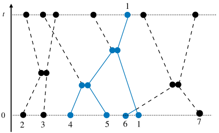
Figure 5: On the left, particle trajectories associated with a term of order $n=7$ in (84) are depicted and the corresponding ordered graph $\overline{\mathcal{T}}_{\prec}$ is depicted on the right : each edge has an order and a sign $\pm$ to record if it is a collision or an overlap. The relevant part $\mathcal{A}$ of the trajectories, which determine ${\textbf{z}}_{1}(t)$, is represented by blue lines and the edges which can be neglected by dashed lines. Ultimately the initial coordinates of the particles in the blue tree $\mathcal{A}$ and the sign of the clusterings prescribe ${\textbf{z}}_{1}(t)$.

Given $\mathcal{A}\in\boldsymbol{\mathcal{A}}_{n}^{\prec,\pm}$, let $\overline{\mathcal{T}}_{\prec}$ be a tree in which $\mathcal{A}$ can be embedded but which has at least one more edge than $\mathcal{A}$. Choosing one leaf in $\overline{\mathcal{T}}_{\prec}$ which is not in $\mathcal{A}$, one can build another tree $\overline{\mathcal{T}}_{\prec}^{\prime}$ by simply changing the sign of the edge connecting this leaf. This changes the tree locally without influencing the value of $h\big{(}{\textbf{z}}_{1}(t)\big{)}$ so that

$$\int dx_{1}\;d\mu_{{\rm sing},\overline{\mathcal{T}}_{\prec}^{\prime}}^{[0,t]}\left({\textbf{Z}}_{n}\right)\;h\big{(}{\textbf{z}}_{1}(t)\big{)}\;\prod_{i=1}^{n}f^{0}\big{(}{\textbf{z}}_{i}(0)\big{)}=-\int dx_{1}\;d\mu_{{\rm sing},\overline{\mathcal{T}}_{\prec}}^{[0,t]}\left({\textbf{Z}}_{n}\right)\;h\big{(}{\textbf{z}}_{1}(t)\big{)}\;\prod_{i=1}^{n}f^{0}\big{(}{\textbf{z}}_{i}(0)\big{)}.$$ (85)

Thus the sum (84) reduces to

$$\lim_{{\varepsilon}\to 0}\mathbb{E}_{\varepsilon}\left[\pi^{\varepsilon}_{t}(h)\right]=\sum_{n=1}^{\infty}\frac{1}{(n-1)!}\sum_{\mathcal{A}\in\boldsymbol{\mathcal{A}}_{n}^{\prec,\pm}}\int dx_{1}\;d\mu_{{\rm sing},\mathcal{A}}^{[0,t]}\left({\textbf{Z}}_{n}\right)\;h\big{(}{\textbf{z}}_{1}(t)\big{)}\;\prod_{i=1}^{n}f^{0}\big{(}{\textbf{z}}_{i}(0)\big{)}.$$

Note that the time ordering of the edges is sufficient to recover from $\mathcal{A}$ the final position ${\textbf{z}}_{1}(t)$. Relabelling the vertices according to the backward order of clusterings, and denoting by $\boldsymbol{\hat{A}}_{n}^{\prec,\pm}$ the set of rooted trees with ordered and signed edges, we finally obtain

$$\lim_{{\varepsilon}\to 0}\mathbb{E}_{\varepsilon}\left[\pi^{\varepsilon}_{t}(h)\right]=\sum_{n=1}^{\infty}\sum_{\hat{\mathcal{A}}\in\boldsymbol{\hat{A}}_{n}^{\prec,\pm}}\int dx_{1}\;d\mu_{{\rm sing},\hat{\mathcal{A}}}^{[0,t]}\left({\textbf{Z}}_{n}\right)\;h\big{(}{\textbf{z}}_{1}(t)\big{)}\;\prod_{i=1}^{n}f^{0}\big{(}{\textbf{z}}_{i}(0)\big{)}.$$ (86)

This defines, by duality, $g(t,z)$ the typical distribution of a particle at time $t$ by imposing a constraint on the final coordinates

$$g(t,z)=\sum_{n=1}^{\infty}\sum_{\hat{\mathcal{A}}\in\boldsymbol{\hat{A}}_{n}^{\prec,\pm}}\int d\mu_{{\rm sing},\hat{\mathcal{A}}}^{[0,t]}\left({\textbf{Z}}_{n}\right)\;\delta_{z-{\textbf{z}}_{1}(t)}\;\prod_{i=1}^{n}f^{0}\big{(}{\textbf{z}}_{i}(0)\big{)},$$ (87)

where the degree of freedom of the initial position $x_{1}$ is fixed by the constraint at time $t$.

To give a meaning to the singularity in the collision operator of the Boltzmann equation (79), some regularity properties on $g$ will be needed. For this we suppose, for a moment, that the initial distribution $f^{0}$ satisfies the following additional smoothness assumption for any $\ell\leq d+1$

$$\forall z\in{\mathbb{T}}^{d}\times\mathbb{R}^{d},\qquad|\partial_{x_{i_{1}}}\dots\partial_{x_{i_{\ell}}}f^{0}(z)|\leq C\mathcal{M}_{\beta/2}(v).$$ (88)

We can then deduce that $g$ is continuous.

Lemma IV.2

Assuming (88), then the density $(x,v)\mapsto g\big{(}t,(x,v)\big{)}$ belongs to $C^{0}_{x}\big{(}{\textbf{M}}^{1}_{v}\big{)}$ for all $t\in[0,T]$, where ${\textbf{M}}^{1}_{v}$ is the space of measures such that $(1+|v|)$ is integrable.

The derivation of this lemma is postponed until the end of the proof of Proposition IV.1. Note that assumption (88) will be lifted at the end of the proof by a density argument.

Step 2 : Identification of the Boltzmann equation.

We are going to check that $g$ is a mild solution of the form (79). For this, it is convenient to interpret the series (87) defining $g(t,z)$ as a backward evolution. This point of view coincides with the standard notion of pseudo-trajectories used to derive Lanford’s Theorem (see e.g. Cercignani_Illner_Pulvirenti ). Fixing at time $t$ the position $z={\textbf{z}}_{1}(t)$ of particle $1$, the collision tree $\hat{\mathcal{A}}$ is built backward by adding the particles which are interacting dynamically with particle $1$ (cf. Figure 5). Proceeding from time $t$, particle $1$ follows the backward free flow either up to time 0 or up to a time $\tau$ at which a branching occurs, say with particle 2. The corresponding edge in the tree $\hat{\mathcal{A}}$ is associated with a sign $-$ if this event is an overlap and $+$ if it is a collision (in which case scattering occurs). Removing this edge splits $\hat{\mathcal{A}}$ into two smaller trees $\hat{\mathcal{A}}_{1},\hat{\mathcal{A}}_{2}$, containing respectively $1$ and $2$, which encode the rest of the trajectory on $[0,\tau]$. Thus the singular measure on $[0,t]$ is the product of the singular measures of the two trees in $[0,\tau]$ with the constraint ${\textbf{x}}_{1}(\tau)={\textbf{x}}_{2}(\tau)$

$$\mu_{{\rm sing},\hat{\mathcal{A}}}^{[0,t]}\left({\textbf{Z}}_{n}\right)=\mu_{{\rm sing},\hat{\mathcal{A}}_{1}}^{[0,\tau]}\left({\textbf{Z}}_{n_{1}}\right)\mu_{{\rm sing},\hat{\mathcal{A}}_{2}}^{[0,\tau]}\left({\textbf{Z}}_{n_{2}}\right)\;s\big{(}({\textbf{v}}_{1}(\tau^{+})-{\textbf{v}}_{2}(\tau^{+}))\cdot\omega\big{)}_{+}\delta_{{\textbf{x}}_{1}(\tau)-{\textbf{x}}_{2}(\tau)}\;d\tau\;d\omega,$$

where $\omega$ is the scattering parameter for the last encounter at time $\tau$ which can be a collision or an overlap according to $s=\pm 1$. We therefore distinguish the velocities at times $\tau^{+}$ and $\tau^{-}$. In this way, (87) can be rewritten

$$g(t,z)=f^{0}\big{(}x-vt,v\big{)}+\sum_{s=\pm 1}\sum_{n_{1},n_{2}=1}^{\infty}\sum_{\hat{\mathcal{A}}_{1}\in\boldsymbol{\hat{A}}_{n_{1}}^{\prec,\pm}\atop\hat{\mathcal{A}}_{2}\in\boldsymbol{\hat{A}}_{n_{2}}^{\prec,\pm}}\int d\tau\;d\omega \int d\mu_{{\rm sing},\hat{\mathcal{A}}_{1}}^{[0,\tau]}\left({\textbf{Z}}_{n_{1}}\right)\;d\mu_{{\rm sing},\hat{\mathcal{A}}_{2}}^{[0,\tau]}\left({\textbf{Z}}_{n_{2}}\right)\;\delta_{(x-v(t-\tau),v)-{\textbf{z}}_{1}(\tau)}\;\delta_{{\textbf{x}}_{1}(\tau)-{\textbf{x}}_{2}(\tau)}$$

$$\times\;s\big{(}({\textbf{v}}_{1}(\tau^{+})-{\textbf{v}}_{2}(\tau^{+}))\cdot\omega\big{)}_{+}\;\prod_{i=1}^{n_{1}+n_{2}}f^{0}\big{(}{\textbf{z}}_{i}(0)\big{)}.$$

In the integral, the free transport operator during time $t-\tau$ can be identified. Depending on $s=\pm 1$, the velocities $(v,v_{2})$ at time $\tau^{+}$ may change at $\tau^{-}$. Thus we define

$$(v^{s},v_{2}^{s})=\begin{cases}(v^{\prime},v_{2}^{\prime}),\qquad&\text{if $s=1$ (scattering occurs at the collision with deflection angle $\omega$)},\\ (v,v_{2}),\qquad&\text{if $s=-1$ (the velocities are unchanged by the overlap)}.\end{cases}$$

Using the uniform convergence of the series, Fubini’s theorem applies

$$g(t,z)=f^{0}\big{(}x-vt,v\big{)}+\sum_{s=\pm 1}\int d\tau\;d\omega\;dv_{2}\;s\big{(}({v}_{1}-{v}_{2})\cdot\omega\big{)}_{+}$$

$$\times\left(\sum_{n_{1}=1}^{\infty}\sum_{\hat{\mathcal{A}}_{1}\in\boldsymbol{\hat{A}}_{n_{1}}^{\prec,\pm}}\int d\mu_{{\rm sing},\hat{\mathcal{A}}_{1}}^{[0,\tau]}\left({\textbf{Z}}_{n_{1}}\right)\;\delta_{(x-v(t-\tau),v^{s})-{\textbf{z}}_{1}(\tau^{-})}\;\prod_{i=1}^{n_{1}}f^{0}\big{(}{\textbf{z}}_{i}(0)\big{)}\right)$$

$$\times\left(\sum_{n_{2}=1}^{\infty}\sum_{\hat{\mathcal{A}}_{2}\in\boldsymbol{\hat{A}}_{n_{2}}^{\prec,\pm}}\int d\mu_{{\rm sing},\hat{\mathcal{A}}_{2}}^{[0,\tau]}\left({\textbf{Z}}_{n_{2}}\right)\;\delta_{(x-v(t-\tau),v_{2}^{s})-{\textbf{z}}_{2}(\tau^{-})}\;\;\prod_{i=1}^{n_{2}}f^{0}\big{(}{\textbf{z}}_{i}(0)\big{)}\right)$$

and the product of the densities $g(\tau^{-})$ can be recovered. The densities are independent as they are defined by different sets of parameters. The continuity, derived in Lemma IV.2, allows us to make sense of the Dirac condition on the positions at time $\tau$. The gain and loss terms in the collision operator arise from the parameter $s=\pm$. Thus $g$ solves the mild form (79) of the Boltzmann equation.

To conclude the proof of Proposition IV.1, it remains to show that the regularity assumption (88) on the initial data is not necessary. Indeed the limiting density $g$ introduced in (87) remains well defined as a measure which can be approximated by a sequence $(g^{\delta})_{\delta>0}$ obtained by regularising $f^{0}$ by smooth densities $f^{0,\delta}$ satisfying (88). By the previous argument each $g^{\delta}$ is a mild solution of the Boltzmann equation and the stability of the Boltzmann equation with respect to uniform convergence implies that the limit $g$ solves also (79). This completes the derivation of Proposition IV.1.

Proof of Lemma IV.2.

First note that the integrability condition can be deduced from the assumption (17) as the test functions are allowed to diverge as $v^{2}$. To prove the statement on the continuity with respect to $x$, let us first recall that the measure $\mu_{{\rm sing},\hat{\mathcal{A}}}^{[0,t]}$ prescribes a set of trajectories ${\textbf{Z}}_{n}([0,t])$ which can be moved rigidly by shifting the root $y$ without changing the weights in the measure. Thus the final condition ${\textbf{x}}_{1}(t)=x$ can be rewritten as a condition on the initial position $x_{1}=x+Y({\textbf{Z}}_{n}([0,t]))$ where the last term (which will not be computed here) depends only on the internal structure of the rigid cluster. For any $r\in{\mathbb{T}}^{d}$, the spatial shift operator $\tau_{r}$ applied to the test function $h$ is defined by $\tau_{r}h(x)=h(x-r)$. A shift by $r$ of the test function can be interpreted by duality by shifting rigidly by $-r$ the whole trajectory ${\textbf{Z}}_{n}([0,t])$ so that

$$\int dxdv\,g\big{(}t,(x,v)\big{)}\,\tau_{r}h(x,v)=\sum_{n=1}^{\infty}\sum_{\hat{\mathcal{A}}\in\boldsymbol{\hat{A}}_{n}^{\prec,\pm}}\int dx_{1}\;d\mu_{{\rm sing},\hat{\mathcal{A}}}^{[0,t]}\left({\textbf{Z}}_{n}\right)\;h\big{(}{\textbf{z}}_{1}(t)\big{)}\;\prod_{i=1}^{n}f^{0}\big{(}{\textbf{z}}_{i}(0)+(r,0)\big{)}$$ (89)

where the shift is only felt at the level of the initial measure. This boils down to applying a shift $\tau_{-r}$ to the function

$$x\mapsto\Gamma_{{\textbf{Z}}_{n}(0)}(x):=\prod_{i=1}^{n}f^{0}\big{(}{\textbf{z}}_{i}(0)+(x,0)\big{)}$$ (90)

whose derivatives of order $d+1$ are bounded thanks to (88) with a growth as $n^{d+1}$. Thus, using the discrete derivative $\tau_{r}-\text{Id}$, we deduce that uniformly in $r$

$$\left|\int dxdv\,g\big{(}t,(x,v)\big{)}\;\frac{1}{r^{d+1}}(\tau_{r}-\text{Id})^{d+1}h(x,v)\right|\leq C\;\Big{\|}\frac{h}{1+|v|}\Big{\|}_{\infty}.$$ (91)

This implies that $d+1$ space derivatives of $g$ are measures in $x$ with values in ${\textbf{M}}^{1}_{v}$, hence $g$ is continuous in $x$ with values in ${\textbf{M}}^{1}_{v}$.

IV.2 The dynamical cluster process

The cluster paths play a key role in the cluster expansion of the exponential moment and it is interesting to study the dynamics of these cluster paths in its own right as a relevant observable of the hard sphere dynamics. The methods developed in this paper provide a direct way for studying the particle trajectories as the exponential moments encode the statistics of the cluster paths. In particular, an analogous result to Proposition IV.1 can be derived at the level of clusters. Before stating it, let us fix some notations.

Following Definition III.3, a limiting cluster path of size $n$ is determined by a decorated cluster (tree) graph

$$\left(n,\mathcal{T}_{\prec},y,V_{n},\Theta_{n-1},\Omega_{n-1}\right)\in{\large\Xi}:=\bigcup_{n\in\mathbb{N}}\{n\}\times\boldsymbol{\mathcal{T}}_{n}^{\prec}\times{\mathbb{T}}^{d}\times\mathbb{R}^{dn}\times(0,\infty)_{s}^{n-1}\times\mathbb{S}^{(d-1)(n-1)},$$ (92)

where $(0,\infty)_{s}^{n-1}$ is a shorthand notation for the simplex $0<\tau_{1}<\tau_{2}<\dots<\tau_{n-1}$. By abuse of notation, we shall use in this section the symbol $\lambda$ for elements in ${\large\Xi}$. Notice that there is no restriction on time in (92), nevertheless it will be convenient to define the notion of cluster paths formed in the time interval $[0,t]$ by the additional constraint $\tau_{n-1}\leq t$. We further recall that, for limiting cluster paths on $[0,T]$, (92) provides a convenient way to parametrise the test functions $H$ defined at the level of (17); we shall write below $H=H(\lambda),\lambda\in{\large\Xi}$ for such parametrization.

Consider two limiting cluster paths formed in the time interval $[0,t]$, with decorated graphs

$$\lambda_{1}=(n_{1},\mathcal{T}_{\prec,1},y_{1},V_{n_{1}},\Theta_{n_{1}-1},\Omega_{n_{1}-1})\quad\text{and}\quad\lambda_{2}=(n_{2},\mathcal{T}_{\prec,2},y_{2},V_{n_{2}},\Theta_{n_{2}-1},\Omega_{n_{2}-1})$$

(such that $\Theta_{n_{1}-1},\Theta_{n_{2}-1}$ are restricted to $(0,t)$). By definition, a collision at time $t$ with deflection angle $\omega$ between particles $i\leq|\lambda_{1}|$ and $j\leq|\lambda_{2}|$ gives rise to the merging of $\lambda_{1},\lambda_{2}$ creating the limiting cluster path with decorated graph

$$[\lambda_{1}\wedge\lambda_{2}]^{i,j,t,\omega}:=\big{(}n_{1}+n_{2},\mathcal{T}_{\prec}^{i,j},y,V_{n_{1}+n_{2}},\Theta_{n_{1}+n_{2}-1},\Omega_{n_{1}+n_{2}-1}\big{)}$$ (93)

built as follows :

• $\Theta_{n_{1}+n_{2}-1}$ contains the reordered collision times of $\lambda_{1},\lambda_{2}$ as well as the time $t$ of the new collision,

• the tree $\mathcal{T}_{\prec}^{i,j}$ is the aggregation of the trees $\mathcal{T}_{\prec,1}$ and $\mathcal{T}_{\prec,2}$ obtained by creating a new edge $\{i,j\}$. The edges of $\mathcal{T}_{\prec}^{i,j}$ are ordered according to the collision times in $\Theta_{n_{1}+n_{2}-1}$,

• the root $y$ corresponds to the center of mass of the initial positions of the cluster $[\lambda_{1}\wedge\lambda_{2}]^{i,j,t,\omega}$, and the initial (reordered) velocities are indicated by $V_{n_{1}+n_{2}}$,

• the velocities of particles $i,j$ are scattered at time $t$ and the deflection angle $\omega$ associated with the new edge $\{i,j\}$ is added to the previous collection of deflection angles to create $\Omega_{n_{1}+n_{2}-1}$.

By construction, the new cluster path is symmetric with respect to $\lambda_{1},\lambda_{2}$.

Theorem IV.3

Let $T>0$ be the convergence time obtained in Proposition II.6. Then for any $t\leq T$, there is a measure $\boldsymbol{\Upsilon}_{t}$ on ${\large\Xi}$ (defined explicitly in (97)) such that the empirical measure on the cluster paths converges to $\boldsymbol{\Upsilon}_{t}$ in the following sense : for any test function $H$ satisfying (17)-(18) and ${\delta}>0$

$$\mathbb{P}_{\varepsilon}\left(\Big{|}\Pi^{\varepsilon}_{t}(H)-\int_{\large\Xi}d\boldsymbol{\Upsilon}_{t}(\lambda_{1})H(\lambda_{1})\Big{|}>\delta\right)\xrightarrow[\mu_{\varepsilon}\to\infty]{}0,$$ (94)

where the test functions on the limiting cluster paths can be parametrised as in (92).

Furthermore, under the regularity assumption (88) for $f^{0}$, the limiting measure obeys an evolution equation which is the counterpart of (79) at the level of cluster paths

$$\forall t\leq T,\quad \int d\boldsymbol{\Upsilon}_{t}(\lambda_{1})H(\lambda_{1})=\int d\boldsymbol{\Upsilon}_{0}(\lambda_{1})H(\lambda_{1})$$ (95)

$$\quad+\frac{1}{2}\int d\tau\,d\omega\,d\boldsymbol{\Upsilon}_{\tau}(\lambda_{1})\,d\boldsymbol{\Upsilon}_{\tau}(\lambda_{2})\sum_{i\in\lambda_{1}\atop j\in\lambda_{2}}\Big{(}H\big{(}[\lambda_{1}\wedge\lambda_{2}]^{i,j,\tau,\omega}\big{)}-H(\lambda_{1})-H(\lambda_{2})\Big{)}\,\delta_{{\textbf{x}}_{i}(\tau)-{\textbf{x}}_{j}(\tau)}\,\big{(}({\textbf{v}}_{i}(\tau)-{\textbf{v}}_{j}(\tau))\cdot\omega\big{)}_{+},$$

where the clusters appearing in the argument of $H$ are formed in the time interval $[0,\tau]$ and merged at time $\tau\in[0,t]$.

The singularity of the Dirac mass in the integral (95) makes sense thanks to the continuity of measures with respect to their roots which can be derived as in Lemma IV.2. We expect the coagulation equation (95) to be stable and that Theorem IV.3 holds without the smoothness assumption (88).

Notice that the time-zero term in (95) is given by

$$\int d\boldsymbol{\Upsilon}_{0}(\lambda_{1})H(\lambda_{1})=\int dz\,f^{0}(z)\,H((x+sv,v)_{s\in[0,T]})$$

and that the equation is complemented with the condition $d\boldsymbol{\Upsilon}_{t}(\lambda)=0$ for $t<\tau_{n-1}$ when $|\lambda|=n$.

Formally, the evolution equation (95) is characteristic of a coagulation process (see e.g. Norris_clusters ). The limiting particle process behaves as a coagulation process at the level of the cluster paths with aggregation rates depending on the law of the process itself. It would be interesting to derive a martingale interpretation of the coagulation process in the spirit of Tanaka’s process Tanaka (see also the surveys Sznitman_saint_flour ; Meleardsurvey ), which describes the typical evolution of a particle velocity associated with the homogeneous Boltzmann equation.

Proof of Theorem IV.3

As in the proof of Proposition IV.1, the concentration estimate (56) implies that the convergence in probability (94) will simply follow from the convergence of the expectation $\mathbb{E}_{\varepsilon}\left[\Pi^{\varepsilon}_{[0,T]}(H)\right]$ defined in (52). This limit can be deduced by Proposition III.4 after a suitable change of variables

$$\lim_{\mu_{\varepsilon}\to\infty}\mathbb{E}_{\varepsilon}\left[\Pi^{\varepsilon}_{[0,T]}(H)\right]=\int d\boldsymbol{\Upsilon}_{T}(\lambda_{1})H(\lambda_{1}),$$ (96)

where $\lambda_{1}$ is indexed by the parameters of the form (92) and the limiting distribution of a typical cluster path follows from (53)

$$d\boldsymbol{\Upsilon}_{T} (\lambda_{1})=d\nu_{T}^{(0)}(\lambda_{1})$$ (97)

$$+\sum_{k\geq 2}\frac{(-1)^{k-1}}{(k-1)!}\sum_{\mathcal{T}^{ov}_{\prec}}d\nu_{T}^{(0)}(\lambda_{1})\int d\Theta_{k-1}\;d\Omega_{k-1}d\tilde{\nu}_{T}^{(0)}(\lambda_{2})\dots d\tilde{\nu}_{T}^{(0)}(\lambda_{k})\prod_{e=\{i,j\}\in E(\mathcal{T}_{\prec}^{ov})}\big{(}({\textbf{v}}_{i}(\tau_{e})-{\textbf{v}}_{j}(\tau_{e}))\cdot\omega_{e}\big{)}_{+}\,\delta_{{\textbf{x}}_{i}(\tau_{e})-{\textbf{x}}_{j}(\tau_{e})}.$$

The subscript $T$ stresses that the collision times and the overlap times belong to the time interval $[0,T]$. Note that the remaining translational degree of freedom is now fixed by the root of $\lambda_{1}$. The previous representation remains valid at time $t\in[0,T]$ : the distribution of the process, denoted by $\boldsymbol{\Upsilon}_{t}$, is obtained by restricting formula (97) to the cluster paths formed during the time interval $[0,t]$

$$\lim_{\mu_{\varepsilon}\to\infty}\mathbb{E}_{\varepsilon}\left[\Pi^{\varepsilon}_{[0,t]}(H)\right]=\int d\boldsymbol{\Upsilon}_{t}(\lambda_{1})H(\lambda_{1}).$$ (98)

This completes the proof of the convergence in probability (94).

We are going to derive (95) and show that this limiting structure can be interpreted as a coagulation process at the level of the cluster paths. We follow a strategy similar to one of the proof of Proposition IV.1 : we first simplify the measure $d\boldsymbol{\Upsilon}_{T}$ and then identify the coagulation equation.

Step 1 : Restriction to a relevant time ordered path structure.

First, we are going to simplify the series (97) by keeping only the relevant cluster overlaps needed to determine the structure of $\lambda_{1}$ (see Figure 6). Given $\mathcal{T}_{\prec}^{ov}$ with edges ordered according to the overlap times, we build a growing collection of trees $\mathcal{A}_{1}\subset\mathcal{A}_{2}\subset\dots$ as follows. Starting from the vertex $\mathcal{A}_{1}=\{1\}$ associated with $\lambda_{1}$, all the vertices and edges connected to $1$ are added to form the set $\mathcal{A}_{2}$. Suppose that $\ell$ belongs to $\mathcal{A}_{2}$ and that the edge $\{1,\ell\}$ has order $k$, then all the neighbours of $\ell$ are added to $\mathcal{A}_{3}$ provided they are linked to $\ell$ by an edge with an order smaller than $k$, i.e. if the corresponding overlap has occurred before $k$. Iterating this procedure leads to an ordered tree $\mathcal{A}$ indexing a set of relevant cluster paths (see Figure 6).

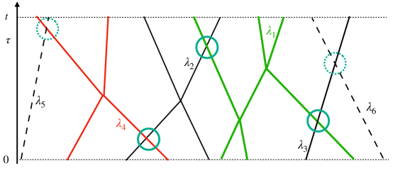
Figure 6: On the left, $6$ cluster paths are depicted and the circles indicate the overlaps between the cluster paths. The corresponding overlap graph $\mathcal{T}_{\prec}^{ov}$ is depicted on the right : the relevant part $\mathcal{A}$ of the overlap graph $\mathcal{T}_{\prec}^{ov}$ is represented by thick lines and the edges which can be neglected by dashed lines. The edges are associated with the circles representing the overlaps on the left figure. The last relevant overlap occurs at time $\tau$ between $\lambda_{1}$ and $\lambda_{2}$.

Finally, we consider the cluster paths indexed by $\mathcal{A}$ only up to the overlap time as explained in Figure 7. This reduced description is sufficient to compute the terms of the series (97). Indeed the branchings and the overlaps which have been discarded compensate as in Formula (85).

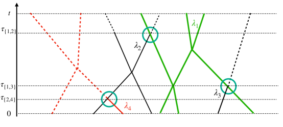
Figure 7: After removing the non necessary overlaps as in Figure 6, the remaining cluster paths have been restricted to the time intervals before the overlap times. Note that the number of particles in the cluster path might be reduced by this procedure : in the case of $\lambda_{4}$, depicted above, the branching beyond the overlap time $\tau_{\{2,4\}}$ is discarded so that the forest $\lambda_{4}$ in the time interval $[0,\tau_{\{2,4\}}]$ has only one particle. Ultimately, the restricted cluster paths, represented with plain lines, are sufficient to compute the coefficients in the series decomposition of $\boldsymbol{\Upsilon}_{t}(\lambda_{1})$.

By analogy with the proof of Proposition IV.1, we denote by $\boldsymbol{\mathcal{A}}_{k}^{\prec}$ the set containing the trees with $k$ vertices of the previous form, i.e. the trees rooted in the vertex indexing $\lambda_{1}$ such that the edge orders are decreasing when examined from the root to a leaf. In summary, to reconstruct $\lambda_{1}$, it is enough to prescribe a tree $\mathcal{A}$ in $\boldsymbol{\mathcal{A}}_{k}^{\prec}$, an ordered collection $\Theta_{k-1}$ of overlapping times and $\Omega_{k-1}$, the associated collection of deflection parameters. The distribution (97) of $\lambda_{1}$ can be rewritten for $t\leq T$ as

$$d\boldsymbol{\Upsilon}_{t} (\lambda_{1})=d\nu_{t}^{(0)}(\lambda_{1})$$ (99)

$$+\sum_{k\geq 2}(-1)^{k-1}\sum_{\mathcal{A}\in\boldsymbol{\mathcal{A}}_{k}^{\prec}}d\nu_{t}^{(0)}(\lambda_{1})\int d\Theta_{k-1}\;d\Omega_{k-1}d\tilde{\nu}_{\tau_{2}}^{(0)}(\lambda_{2})\dots d\tilde{\nu}_{\tau_{k}}^{(0)}(\lambda_{k})\prod_{e=\{i,j\}\in E(\mathcal{A})}\big{(}({\textbf{v}}_{i}(\tau_{e})-{\textbf{v}}_{j}(\tau_{e}))\cdot\omega_{e}\big{)}_{+}\,\delta_{{\textbf{x}}_{i}(\tau_{e})-{\textbf{x}}_{j}(\tau_{e})}.$$

Note that the factor $1/(k-1)!$ in (97) is no longer needed as the cluster paths are indexed by the time ordering. This is the counterpart of Formula (87) for the particle density.

Step 2 : Identification of the coagulation equation.

From (99), we are now going to derive (95) which is stated below in an asymmetric way

$$\int d\boldsymbol{\Upsilon}_{t}(\lambda_{1})H(\lambda_{1})= \int d\boldsymbol{\Upsilon}_{0}(\lambda_{1})H(\lambda_{1})$$ (100)

$$+\int d\tau\,d\omega\,d\boldsymbol{\Upsilon}_{\tau}(\lambda_{1})\,d\boldsymbol{\Upsilon}_{\tau}(\lambda_{2})\sum_{i\in\lambda_{1}\atop j\in\lambda_{2}}\Big{(}\frac{1}{2}H\big{(}[\lambda_{1}\wedge\lambda_{2}]^{i,j,\tau,\omega}\big{)}-H(\lambda_{1})\Big{)}\,\delta_{{\textbf{x}}_{i}(\tau)-{\textbf{x}}_{j}(\tau)}\,\big{(}({\textbf{v}}_{i}(\tau)-{\textbf{v}}_{j}(\tau))\cdot\omega\big{)}_{+}\;.$$

Consider the terms in the series (99) with at least one overlap ($k\geq 2$) or such that $|\lambda_{1}|\geq 2$. Then starting from time $t$ and looking backward at the trajectories of $\lambda_{1}$ and at the overlap times $\Theta_{k-1}$, we denote by $\tau$ the first time at which a collision or an overlap occur.

• If an overlap occurs at time $\tau$, then the trajectory of $\lambda_{1}$ is unchanged at time $\tau$ so that the restriction of the cluster path from $[0,t]$ to $[0,\tau]$ is still given by the same set of parameters of the form (92). Splitting the tree $\mathcal{A}$ (coding the overlaps) into two parts containing respectively $\lambda_{1}$ and $\lambda_{2}$, the cluster paths overlapping $\lambda_{1}$ during $[0,\tau]$ (resp $\lambda_{2}$) can be grouped to reconstruct the distributions $\boldsymbol{\Upsilon}_{\tau}(\lambda_{1})$ (resp $\boldsymbol{\Upsilon}_{\tau}(\lambda_{2})$). In this way, the loss term in (100) is recovered.

• If a collision in $\lambda_{1}$ occurs at time $\tau$ between particles $i$ and $j$ with deflection parameter $\omega$, the collision tree $\mathcal{T}_{\prec}$ associated with $\lambda_{1}$ can be split into two parts $\mathcal{T}_{\prec,1}$ and $\mathcal{T}_{\prec,2}$ defining two cluster paths $\lambda_{1}^{\prime},\lambda_{2}^{\prime}$ so that, by the definition (93),

  $$\lambda_{1}=[\lambda_{1}^{\prime}\wedge\lambda_{2}^{\prime}]^{i,j,\tau,\omega}.$$ (101)

  Proceeding as before and regrouping the cluster paths overlapping $\lambda_{1}^{\prime}$ and $\lambda_{2}^{\prime}$, the distributions $\boldsymbol{\Upsilon}_{\tau}(\lambda_{1}^{\prime}),\boldsymbol{\Upsilon}_{\tau}(\lambda_{2}^{\prime})$ can be identified. The factor $1/2$ is necessary as the splitting of $\lambda_{1}$ is symmetric. Changing variables from $\lambda_{1}^{\prime},\lambda_{2}^{\prime}$ to $\lambda_{1},\lambda_{2}$, this leads to the gain term in (100).

Proposition IV.3 is therefore complete.

References

- [1] S. Albeverio, B. Rüdiger, and P. Sundar. The Enskog process. J. Stat. Phys., 167(1):90–122, 2017.
- [2] R. K. Alexander. The infinite hard-sphere system. PhD thesis, University of California, Berkeley, 1975.
- [3] T. Bodineau, I. Gallagher, and L. Saint-Raymond. Derivation of an Ornstein-Uhlenbeck process for a massive particle in a rarified gas of particles. Annals of IHP, 19(6):1647–1709, 2018.
- [4] T. Bodineau, I. Gallagher, L. Saint-Raymond, and S. Simonella. One-sided convergence in the Boltzmann–Grad limit. Annales de la Faculté des sciences de Toulouse: Mathématiques, 27(5):985–1022, 2018.
- [5] T. Bodineau, I. Gallagher, L. Saint-Raymond, and S. Simonella. Fluctuation theory in the Boltzmann–Grad limit. Journal of Statistical Physics, 180(1):873–895, 2020.
- [6] T. Bodineau, I. Gallagher, L. Saint-Raymond, and S. Simonella. Long-time correlations for a hard-sphere gas at equilibrium. preprint arXiv:2012.03813, to appear in CPAM, 2020.
- [7] T. Bodineau, I. Gallagher, L. Saint-Raymond, and S. Simonella. Statistical dynamics of a hard sphere gas: fluctuating Boltzmann equation and large deviations. preprint arXiv:2008.10403, 2020.
- [8] T. Bodineau, I. Gallagher, L. Saint-Raymond, and S. Simonella. Dynamics of dilute gases : a statistical approach. arXiv:2201.10149, 2022.
- [9] D. Brydges. A short course on cluster expansions. Elsevier/North Holland, Amsterdam, 1984.
- [10] C. Cercignani, V. I. Gerasimenko, and D. Y. Petrina. Many-particle dynamics and kinetic equations, volume 420 of Mathematics and its Applications. Kluwer Academic Publishers Group, Dordrecht, 1997. Translated from the Russian manuscript by K. Petrina and V. Gredzhuk.
- [11] C. Cercignani, R. Illner, and M. Pulvirenti. The mathematical theory of dilute gases, volume 106 of Applied Mathematical Sciences. Springer-Verlag, New York, 1994.
- [12] R. Denlinger. The propagation of chaos for a rarefied gas of hard spheres in the whole space. Arch. Ration. Mech. Anal., 229(2):885–952, 2018.
- [13] R. Fernández and A. Procacci. Cluster expansion for abstract polymer models. Comm. Math. Phys., 274(1):123–140, 2007.
- [14] S. Friedli and Y. Velenik. Statistical mechanics of lattice systems: a concrete mathematical introduction. Cambridge University Press, 2017.
- [15] A. Gabrielov, V. Keilis-Borok, Y. Sinai, and I. Zaliapin. Statistical properties of the cluster dynamics of the systems of statistical mechanics. In Boltzmann’s legacy. Papers based on the presentations at the international symposium, Vienna, Austria, June 7–9, 2006., pages 203–215. Zürich: European Mathematical Society (EMS), 2008.
- [16] I. Gallagher, L. Saint-Raymond, and B. Texier. From Newton to Boltzmann: hard spheres and short-range potentials. Zürich: European Mathematical Society (EMS), 2014.
- [17] G. Gallavotti, F. Bonetto, and G. Gentile. Aspects of Ergodic, Qualitative and Statistical Theory of Motion. Springer, Berlin, 2004.
- [18] V. Gerasimenko and I. Gapyak. Low-density asymptotic behavior of observables of hard sphere fluids. Adv. Math. Phys., 2018:11, 2018.
- [19] V. I. Gerasimenko and I. V. Gapyak. Boltzmann-Grad asymptotic behavior of collisional dynamics. Rev. Math. Phys., 33(2):32, 2021.
- [20] V. I. Gerasimenko and I. V. Gapyak. Propagation processes of correlations of hard spheres. arXiv:2111.13940, 2021.
- [21] H. Grad. On the kinetic theory of rarefied gases. Commun. Pure Appl. Math., 2:331–407, 1949.
- [22] D. Heydecker and R. I. Patterson. Bilinear coagulation equations. preprint arXiv:1902.07686, 2019.
- [23] R. Illner and M. Pulvirenti. Global validity of the Boltzmann equation for two-and three-dimensional rare gas in vacuum: Erratum and improved result. Commun. Math. Phys., 121(1):143–146, 1989.
- [24] S. Jansen and L. Kolesnikov. Cluster expansions: Necessary and sufficient convergence conditions. arXiv:2112.13134, 2021.
- [25] S. Kaniel and M. Shinbrot. The Boltzmann equation. I. Uniqueness and local existence. Commun. Math. Phys., 58:65–84, 1978.
- [26] R. Kotecký and D. Preiss. Cluster expansion for abstract polymer models. Commun. Math. Phys., 103(491), 1986.
- [27] O. E. Lanford, III. Time evolution of large classical systems, pages 1–111. Lecture Notes in Phys., Vol. 38. 1975.
- [28] K. Matthies and F. Theil. A semigroup approach to the justification of kinetic theory. SIAM J. Math. Anal., 44(6):4345–4379, 2012.
- [29] C. McFadden and L.-S. Bouchard. Universality of cluster dynamics. Phys. Rev. E, 82, 2010.
- [30] S. Méléard. Probabilistic interpretation and approximations of some Boltzmann equations. pages 1–64, 1998.
- [31] J. R. Norris. Cluster coagulation. Commun. Math. Phys., 209(2):407–435, 2000.
- [32] R. I. A. Patterson, S. Simonella, and W. Wagner. Kinetic theory of cluster dynamics. Phys. D: Nonlin. Phen., 335:26–32, 2016.
- [33] R. I. A. Patterson, S. Simonella, and W. Wagner. A kinetic equation for the distribution of interaction clusters in rarefied gases. J. Stat. Phys., 169(1):126–167, 2017.
- [34] O. Penrose. Convergence of fugacity expansions for classical systems. page 101. Benjamin, New York, 1967.
- [35] S. Poghosyan and D. Ueltschi. Abstract cluster expansion with applications to statistical mechanical systems. Journal of mathematical physics, 50(5):053509, 2009.
- [36] M. Pulvirenti, C. Saffirio, and S. Simonella. On the validity of the Boltzmann equation for short range potentials. Rev. Math. Phys., 26(2):1450001, 64, 2014.
- [37] M. Pulvirenti and S. Simonella. On the evolution of the empirical measure for the hard-sphere dynamics. Bull. Inst. Math. Acad. Sin., 10(2):171–204, 2015.
- [38] M. Pulvirenti and S. Simonella. The Boltzmann-Grad limit of a hard sphere system: analysis of the correlation error. Invent. Math., 207(3):1135–1237, 2017.
- [39] D. Ruelle. Statistical mechanics. World Scientific Publishing Co., Inc., River Edge, NJ; Imperial College Press, London, 1999. Rigorous results, Reprint of the 1989 edition.
- [40] S. Simonella. Evolution of correlation functions in the hard sphere dynamics. J. Stat. Phys., 155(6):1191–1221, 2014.
- [41] S. Simonella and R. Winter. Pointwise decay of truncated correlations in chaotic states at low density. arXiv:2012.01246, 2020.
- [42] J. G. Sinaĭ. Construction of the dynamics for one-dimensional systems of statistical mechanics. Teoret. Mat. Fiz., 11(2):248–258, 1972.
- [43] J. G. Sinaĭ. Construction of a cluster dynamic for the dynamical systems of statistical mechanics. Vestnik Moskov. Univ. Ser. I Mat. Meh., 29(1):152–158, 1974. Collection of articles dedicated to the memory of Ivan Georgievič Petrovskiĭ.
- [44] H. Spohn. Fluctuations around the Boltzmann equation. J. Statist. Phys., 26(2):285–305, 1981.
- [45] H. Spohn. Large scale dynamics of interacting particles. Texts and Monographs in Physics. Springer, Heidelberg, 1991.
- [46] A.-S. Sznitman. Topics in propagation of chaos. Lect. Notes Math. Springer, 1991.
- [47] H. Tanaka. Probabilistic treatment of the Boltzmann equation of Maxwellian molecules. Z. Wahrscheinlichkeitstheor. Verw. Geb., 46:67–105, 1978.
- [48] D. Ueltschi. Cluster expansions and correlation functions. Moscow Math. J., 4:511–522, 2004.
- [49] S. Ukai. On the existence of global solutions of mixed problem for non-linear Boltzmann equation. Proc. Japan Acad., 50:179–184, 1974.
- [50] S. Ukai. Les solutions globales de l’équation de Boltzmann dans l’espace tout entier et dans le demi-espace. C. R. Acad. Sci., Paris, Sér. A, 282:317–320, 1976.