Giant Planets from the Inside-Out

Abstract

Giant planets acquire gas, ices and rocks during the early formation stages of planetary systems and thus inform us on the formation process itself. Proceeding from inside out, examining the connections between the deep interiors and the observable atmospheres, linking detailed measurements on giant planets in the solar system to the wealth of data on brown dwarfs and giant exoplanets, we aim to provide global constraints on interiors structure and composition for models of the formation of these planets.

New developments after the Juno and Cassini missions point to both Jupiter and Saturn having strong compositional gradients and stable regions from the atmosphere to the deep interior. This is also the case of Uranus and Neptune, based on available, limited data on these planets. Giant exoplanets and brown dwarfs provide us with new opportunities to link atmospheric abundances to bulk, interior abundances and to link these abundances and isotopic ratios to formation scenarios. Analysing the wealth of data becoming available will require new models accounting for the complexity of the planetary interiors and atmospheres.
 
Revised chapter submitted to Protostars and Planets VII, Editors: Shu-ichiro Inutsuka, Yuri Aikawa, Takayuki Muto, Kengo Tomida, and Motohide Tamura
1 April 2022  
 

1 INTRODUCTION

According to the classical picture, giant planets form from planetary cores made of ices and rocks that grew beyond a critical mass of about 10 times the mass of the Earth, at which point they began accreting hydrogen and helium and increased their mass rapidly (Perri and Cameron, 1974; Mizuno, 1980; Bodenheimer and Pollack, 1986). Their large mass implies a large internal energy reservoir that is released slowly, implying that they are hot, fluid, and mostly convective (Hubbard, 1968; Stevenson and Salpeter, 1977). In parallel, observations of tropospheric temperatures in Jupiter and Saturn show very limited equator-to-pole gradients, despite having a pattern of insolation that is strongly variable from equator to pole, pointing to efficient convective mixing redistibuting energy (Ingersoll and Porco, 1978). This led to today’s models of giant planets (extended to giant exoplanets) made of a central dense core surrounded by a hydrogen-helium envelope of nearly uniform composition, upon which planetary rotation imposes a latitudinally-banded structure in the atmosphere.

Recent observations, in particular by Juno (Bolton et al., 2017b) and Cassini (Spilker, 2019), show that Jupiter and Saturn depart – potentially strongly – from that ideal picture. Both their interiors show signs of strong variations in composition and potentially extended stably stratified regions. The temperatures, composition, and aerosol properties of their atmospheres are non-uniform to great depths (including the deep troposphere) and variable over a variety of timescales linked to seasonal climates and local meteorology. In parallel, the analysis of observations of exoplanets and brown dwarfs also shows signs of this complexity, linked to the presence of clouds, strong horizontal variations in temperature and probably chemical composition and time variability. Linking Solar-System giant planets to exoplanets and brown dwarfs is crucial to better characterize these objects and understand planet formation, and planetary environments, in general. The previous PPVI review chapters on planetary interior structures and giant planet formation (Baraffe et al., 2014; Helled et al., 2014a) focused on evidence available on solar system planets and moons, and on exoplanets based on their mass-radius properties. We now have refined measurements of Jupiter and Saturn’s properties, and are beginning to truly characterise exoplanetary atmospheres. The present chapter is based on this new evidence.

We first present the current understanding of the interiors and atmospheres of Jupiter, Saturn, Uranus and Neptune in § 2. Next, we review constraints on brown dwarfs and giant exoplanets in § 3. In § 4 we apply these findings to the history of the formation planets. In each subsection, we organise our discussion ‘from the inside out’, starting with the deep interior and moving to the regions more readily accessible to remote sensing - the atmospheres. We provide our conclusions in § 5.

2 THE SOLAR SYSTEM GIANT PLANETS

In this section, we discuss our present understanding of the interiors and atmospheres of the giant planets, following the Galileo, Juno, and Cassini orbital remote sensing of Jupiter and Saturn, as well as Voyager-2 observations (and three decades of ground- and space-based astronomy) of Uranus and Neptune. We focus on questions that may have relevance to the characterisation of exoplanets and brown dwarfs in § 3. In particular, how are heat and elements transported in the atmosphere and interior of giant planets? What can be inferred from the observation of their atmosphere? What are the consequences for their evolution? We structure this section by starting in the deep interior, moving upwards into the banded troposphere and the cloud-forming ‘weather layer,’ and finally into the stably-stratified middle atmosphere above the clouds.

2.1 Interior Structure

2.1.1 The core-envelope structure

A lack of constraints and Ockham’s razor have meant that giant planet interiors have long been thought to be relatively simple: A well-defined central core, leftover from the planet’s formation, and a convective mostly homogeneous hydrogen-helium envelope (except for a transition in helium content due to a phase separation in Jupiter and Saturn) on top (see Guillot, 2005; Fortney and Nettelmann, 2010; Helled et al., 2014b, and references therein). Yet, the question of their inherent complexity, including the presence of possible important compositional gradients, was raised already in the 1980’s (Stevenson, 1985). New data show that this complexity must be accounted for.

Spacecraft measurements of the planets’ gravity fields have thus far been the main constraints used for interior models. These measurements have been improved by more than two orders of magnitude thanks to the close-in, polar orbits of Juno at Jupiter (Iess et al., 2018; Durante et al., 2020) and of the Cassini Grand Finale at Saturn (Iess et al., 2019). These measurements led to models showing that Jupiter’s interior is clearly inhomogeneous, with a deep metallic envelope that must be enriched in heavy elements (all elements heavier than hydrogen and helium) compared to its upper molecular envelope, possibly requiring the presence of a fuzzy core that instead of being well-defined extends in the overlaying envelope (Wahl et al., 2017a; Debras and Chabrier, 2019; Ni, 2019; Nettelmann et al., 2021; Miguel et al., 2022). In Saturn, a milestone has been reached thanks to the detection of the normal modes of oscillation of the planet (e.g., Hedman and Nicholson, 2013; Hedman et al., 2019). Seismology has thus provided evidence of the presence of a deep stable region (Fuller, 2014), of substantial helium differentiation leading to the formation of a helium-rich core (Mankovich and Fortney, 2020), and of a gradient in the distribution of heavy elements similar to that inferred in Jupiter and extending to about 60% of Saturn’s radius (Mankovich and Fuller, 2021). In comparison, Uranus and Neptune, which have been briefly visited only by Voyager 2 in 1986 and 1989, respectively, remain much less well characterised (Helled et al., 2020a, and references therein).

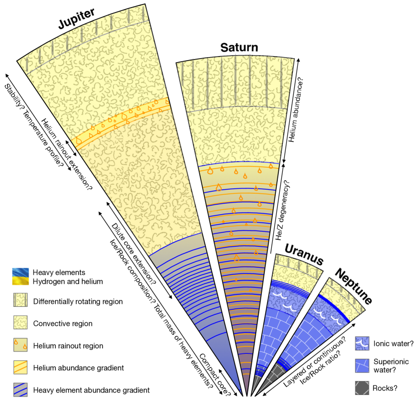
Figure 1: Slices of the internal structures of Jupiter, Saturn, Uranus and Neptune highlighting compositional gradients in helium (orange) and heavy elements (blue). Jupiter and Saturn are characterized by a phase separation of helium in metallic hydrogen starting near Mbar pressures. Juno and Cassini measurements also indicate the presence of a dilute heavy element core in these planets, implying that heavy elements are partially mixed with hydrogen and helium rather forming separate pure layers. In these planets, each layer correspond to a 2% increase of the helium/hydrogen ratio (orange) or of the heavy element mass fraction $Z$ (blue). For Uranus and Neptune, a structure dominated by well-separated layers, including a solid superionic water layer is presented but solutions with compositions that evolve more continuously are also highly plausible (see text).

Fig. 1 sketches the interior structures of the four giant planets, as envisioned from the latest available publications. Jupiter is thus made of a central dense compact core of small mass (less than about 6$\,\rm M_{\oplus}$, possibly zero), probably a dilute core extending to possibly a high fraction ($\sim 50\%$) of the planet’s radius, an inner envelope of high helium abundance and an outer envelope with a low helium abundance (Miguel et al., 2022). A region of variable helium abundance in which helium droplets should form is sandwiched between the inner and outer envelope. It extents to up to 8% of the planet in radius (Mankovich and Fortney, 2020) but could be smaller, depending on the temperature profile in the region. The dilute core is believed to have a variable composition, from up to perhaps $50\%$ of heavy elements in the deep regions down to $\approx 8\%$ when merging with the inner envelope (and the complement in hydrogen and helium). Although Jupiter has a high intrinsic luminosity (Li et al., 2018) and should be largely convective (e.g., Guillot et al., 2004), these zones of variable compositions should be either stable to convection or characterised by double-diffusive convection (e.g. Rosenblum et al., 2011; Leconte and Chabrier, 2012; Wood et al., 2013; Nettelmann et al., 2015). The nature of heavy elements in terms of the fraction of ices, rocks and iron that they contain is unknown.

Saturn has a structure that is qualitatively similar to Jupiter but with important differences. The work of Mankovich and Fuller (2021) which integrates constraints from both gravimetry and seismology assumes no central compact core. The same work provides evidence for the existence of a dilute core with a gradient in both heavy elements and helium abundance extending to 60% of the planet’s radius. The mass of heavy elements involved in this dilute core is constrained to values in the range $15.5-20.8\rm\,M_{\oplus}$. Helium demixing is much more pronounced than in Jupiter, possibly leading to an inner region with less than 5% hydrogen (Mankovich and Fortney, 2020). The upper envelope is homogeneous with a mass fraction of heavy elements $Z=0.028-0.084$.

Uranus and Neptune are of comparatively much smaller mass, with an interior dominated by heavy elements and an even larger variety of possible structures. Uncertainties are large, due both to the loose constraints on the planets’ gravity fields, but also to uncertain rotation rates (Helled et al., 2010, 2011). This allows a full range of solutions for the core ($11-13.3\rm\,M_{\oplus}$ for Uranus, $13-15.5\rm\,M_{\oplus}$ for Neptune). Fully differentiated solutions include a central rock core, a shell of solid super-ionic water and an overlaying layer of fluid ionic water (Redmer et al., 2011; Nettelmann et al., 2013). Recent studies have shown super-ionic water to possess a significant shear modulus which should allow only slow convective motions (Millot et al., 2019) and imply that Uranus and Neptune would progressively solidify with time (Stixrude et al., 2021). However solutions are also possible in which with rocks, ices and even a small fraction ($\lesssim 10\%$) of gas are mixed, potentially modifying these conclusions. In all cases, their overlaying hydrogen-helium-dominated envelopes are relatively small, being only $1.25-3.5\rm\,M_{\oplus}$ for Uranus and $1.6-4.15\rm\,M_{\oplus}$ for Neptune (Helled et al., 2011; Nettelmann et al., 2013; Helled et al., 2020a).

Thus, strong compositional gradients occur in all four giant planets. The gradient in helium composition in Jupiter and Saturn is linked to a phase separation of helium in metallic hydrogen (see § 2.1.2 hereafter). The increase in molecular weight thus formed is strongly stabilising to convection, but it is not yet clear whether this region is stable, diffusive-convective or fully convective (see § 2.1.3). Jupiter and Saturn’s dilute core regions seem at this point to be unrelated to any phase transition, and would rather be a leftover from formation processes (see § 4). These regions should therefore either be diffusive-convective or convectively stable. The existence of an extended region which is stable to convection is demonstrated in Saturn, thanks to seismology and the discovery of oscillation modes mixing fundamental waves (f-modes) and gravity waves (g-modes) (Fuller, 2014), as the latter can only propagate in stable regions. In Uranus and Neptune, the transition from a hydrogen and helium-dominated envelope to a much more dense interior should lead either to diffusive convection or to a stable region in which heat is mainly transported by conduction.

2.1.2 Equations of State and Phase Diagrams

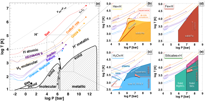
Figure 2: Phase diagrams of key elements with pressure-temperature profiles of relevant astrophysical objects (the Sun, brown dwarfs CoRoT-15b and Gl229 B, giant exoplanet HD 209458 b, and Jupiter, Saturn, Uranus and Neptune). Pressures are in bars ($\rm 1\,bar=10^{5}\,Pa=10^{6}\,dyn/cm^{2}$). (a): Phases of hydrogen, with solid phases shown as a hashed region, critical points as black circles, thick lines indicating a first order (discontinuous) phase transition, and dashed lines a continuous transition (from Guillot and Gautier, 2015). (b): Location of the hydrogen-helium phase separation leading to helium rain-out in Jupiter and Saturn (yellow). The critical demixing temperatures obtained for an 11 mol% He fraction from ab-initio simulations (Schöttler and Redmer, 2018) are shown in orange. Those obtained from high-pressure experiments are shown as two triangles connected by a red curve (Brygoo et al., 2021). The demixing region is extended to high pressure using the fully pressure-ionised limit (Stevenson, 1975). (c): Phase diagram of H₂O, including the fluid molecular, ionic and plasma phases, the solid ice phases and the superionic phase, as labelled (Redmer et al., 2011; Salzmann, 2019; Mazevet et al., 2019a). The H₂O transitions are mostly relevant for Uranus and Neptune and ice giants. The solubility of H₂O in metallic hydrogen at $P\sim 10-100$ Mbar is from Wilson and Militzer (2012). A region of water insolubility in molecular hydrogen is speculated at $P\sim 10-100\,$kbar (Bali et al., 2013; Bailey and Stevenson, 2021) but controversial (Soubiran and Militzer, 2015). (d): Region of iron solidification (from Mazevet et al., 2019b), relevant for the central regions of Jupiter and possibly Saturn. In planetary interiors, iron is believed to be entirely soluble in metallic hydrogen (Wahl et al., 2013) (e): Regions of silicate solidification (from Mazevet et al., 2019b), relevant in the interiors of Uranus, Neptune, Saturn and Jupiter. Note that MgSiO₃ decomposes at high pressures into MgO (which should be solid in Jupiter and Saturn) and SiO₂ (which may still be liquid in the deep interior of Jupiter and Saturn). These two phases have slightly different solubilities but should be both mostly soluble in metallic hydrogen in planetary interiors (González-Cataldo et al., 2014).

For a large part, our knowledge of the interiors of giant planets is inferred from hydrostatic models and equations of state governing the behaviour of matter at pressures reaching $\sim 70\,$Mbar ($\sim 7$ TPa) in Jupiter and even much more in selected brown dwarfs (see Fig. 2a). In this regime, hydrogen transitions from a weakly conducting molecular fluid to a metallic fluid by pressure ionization. In giant planets and brown dwarfs, this transition occurs smoothly around pressures $\sim 1\,$Mbar (Sano et al., 2011; Loubeyre et al., 2012). At temperatures below 4000 K and pressures between 1.5 and 2.5 Mbar, this transition occurs discontinuously (McMahon et al., 2012; Knudson et al., 2015). This regime, as that of the solidification of hydrogen, occurs at too low temperatures to be of relevance for giant planets and brown dwarfs (see Guillot, 2005).

The calculation of an equation of state is difficult, in particular where electrons are partially degenerate and Coulombian interactions are important. The pioneering work of Saumon et al. (1995) included the possibility of a ”Plasma Phase Transition” (PPT) for giant planets and led to a high compressibility of hydrogen, now ruled-out by the experiments. Several equations of state of hydrogen or of the hydrogen-helium mixture solving these issues have become available (Militzer and Hubbard, 2013; Becker et al., 2014; Miguel et al., 2016, 2018; Chabrier et al., 2019). While relying on ab-initio calculations, the difference between them amounts to up to $\sim 8$% in density and $\sim 10$% in temperature on a Jupiter adiabat, at pressures between $\sim 0.03$ to 10 Mbar. This is a significant source of uncertainty which must be accounted for, especially when seeking to reproduce the tight constraints obtained for Jupiter and Saturn.

Helium, shown in Fig. 2b, undergoes a phase separation from metallic hydrogen at temperatures of relevance for Jupiter and Saturn. The formation of helium-rich droplets and their sinking under the action of gravity has strong consequences both for the cooling and the structure of these planets (e.g., Stevenson and Salpeter, 1977; Mankovich and Fortney, 2020). Considerable progress has been made on this issue: Calculations based on first-principle are available and provide the full phase diagram as a function of pressure, temperature and composition (Morales et al., 2013; Schöttler and Redmer, 2018). High-pressure experiments provide direct evidence for immiscibility at Jupiter-interior conditions (Brygoo et al., 2021). Uncertainties remain however: Ab-initio simulations predict that phase separation should occur in Saturn but not necessarily in Jupiter, leading Mankovich and Fortney (2020) to arbitrarily offset the critical temperatures from Schöttler and Redmer (2018) upward by 540 K in order to account for the depleted atmospheric helium abundance (see § 2.4.2). On the other hand, high-pressure experiments using laser-driven shock compression of H₂-He samples that have been pre-compressed in diamond-anvil cells indicate a much higher critical temperature reaching 10,500 K at 1.5 Mbar (Brygoo et al., 2021). Given the importance of the issue for Jupiter and Saturn, further models and experiments are warranted.

Given its high abundance in the Universe, water deserves special consideration. Its phase diagram is shown in Fig. 2c. Importantly, when embedded inside the envelope of a giant planet, water is found to be easily soluble in metallic hydrogen (Wilson and Militzer, 2012), allowing for the possibility of an erosion of such a core (see discussion in § 4.2.2). In Uranus and Neptune, below the hydrogen-helium-dominated envelope, water should be present in the form of a ionic fluid, but could then transition into superionic water (French et al., 2009; Redmer et al., 2011). This phase is a combination of a proton fluid and an oxygen lattice and is thus hybrid between a fluid and a solid, but experiments and ab-initio calculations with density functional theory indicate that it should behave as a solid (Millot et al., 2019). The question of how other elements may affect the picture is not yet clear (e.g., Guarguaglini et al., 2019), especially given that water can dissolve important amounts of MgO (Kim et al., 2021; Nettelmann, 2021).

Interestingly, water may also separate from molecular hydrogen at low pressures: Experiments indicate immiscibility at $17-26$ kbar and temperatures lower than $750-1000$ K (Bali et al., 2013), leading to the possibility that Uranus and Neptune may possess liquid water oceans (Bailey and Stevenson, 2021). This issue is open however for several reasons: The experimental data have to be extrapolated to higher pressures and temperatures in order to meet the conditions relevant for Uranus and Neptune. But more importantly, ab-initio calculations do not find immiscibility in these conditions (Soubiran and Militzer, 2015), raising the possibility that the immiscibility found by Bali et al. (2013) may result from a contamination by the silicates used in the experiments. This issue which has significant consequences for the structures of Uranus, Neptune and ice giants must be investigated further.

Iron, shown in Fig. 2d, has a relatively high melting temperature at high pressures (Mazevet et al., 2019b), and thus should be in solid form in the central regions of Jupiter and Saturn. Nonetheless, ab initio simulations indicate that it is highly soluble in metallic hydrogen (Wahl et al., 2013) and therefore could be eroded if energetically possible.

Finally, Fig. 2e shows a potential phase diagram for silicates, or more precisely, MgSiO₃, expected to transform into MgO and SiO₂ above $\sim 10\,$Mbar (Mazevet et al., 2019b). The melting temperature is relatively high, indicating that MgO (but not SiO₂) should be solid in Jupiter and Saturn’s cores. For the conditions expected in the deep interiors of these planets, both MgO and SiO₂ are expected to be soluble in metallic hydrogen, assuming abundances consistent with a solar composition (González-Cataldo et al., 2014). At lower pressures, MgSiO₃ should be solid in Uranus and Neptune.

In order to understand the formation of giant planets and the fate of their primordial cores, one must consider that they initially formed with significantly higher temperatures ($\sim 30,000K$ or more at Jupiter’s center). Figure 2 shows that during a significant fraction of their evolution, heavy elements in giant planets were entirely fluid and soluble. This does not imply that they were necessarily mixed efficiently, as this depends on whether this was energetically possible (see § 4.2.2). Depending of the elements considered, insolubility or solidification occurred first. For example, helium separation should have occurred first in Saturn after $\sim 1.5\,$Gyr of evolution, then in Jupiter, $\sim 4\,$Gyr after its formation (Mankovich and Fortney, 2020), but helium solidification is beyond reach. Silicates in Jupiter and Saturn’s core may have partially solidified, without becoming insoluble. Water in Uranus and Neptune may have become super-ionic (at high pressures) and may have become insoluble as well (at low pressures).

Representative exoplanets shown in Fig. 2 are fully miscible because of their high entropies, either because they are close to their star, or because they are massive and retained a large fraction of the internal energy. We are however beginning to have the possibility to characterise giant planets with lower entropies. This should enable an extremely useful comparison with solar system giant planets. For example, the issue of helium phase separation should concern planets with masses between about $\sim 40$ and $400\rm\,M_{\oplus}$ and effective temperatures below about $\sim 150\,$K, i.e., weakly irradiated and sufficiently old planets (Fortney and Hubbard, 2004). With the possibility to measure atmospheric compositions (see § 2.3), the existence of phase separations of other elements and of the link between atmospheric and interior composition will become highly significant.

2.1.3 Departures from an Isentropic Interior

Traditionally, models of giant planets have been built with the assumption of an isentropic structure, with the idea that (1) the relatively high intrinsic luminosities coupled to the high radiative and conductive opacities should imply convective interiors and that (2) the superadiabaticity needed to transport the observed heat fluxes is small (see Guillot et al., 2004, and references therein). Since efficient (nearly adiabatic) convection must lead to a uniform composition, this assumption must break down in the presence of compositional gradients, as was in fact recognised early-on for Uranus and Neptune (Podolak et al., 1991; Hubbard et al., 1995).

In the presence of a gradient of mean molecular weight $\nabla_{\mu}\equiv d\log\mu/d\log P$ (where $\mu$ is the mean molecular weight and $P$ the pressure), the temperature gradient $\nabla_{T}\equiv d\log T/d\log P$ (where $T$ is temperature) should satisfy the convective stability criterion (Ledoux, 1947; Kippenhahn and Weigert, 1990):

$$\nabla_{T}\leq\nabla_{\rm ad}+(\varphi/\delta)\nabla_{\mu},$$ (1)

where $\nabla_{\rm ad}\equiv(\partial\log T/\partial\log P)_{S,\mu}$ is the adiabatic gradient assuming uniform composition, $S$ is specific entropy, and $\varphi$ and $\delta$ are dimensionless thermodynamical quantities that are equal to $1$ for a perfect gas ($\varphi=-(\partial\log\rho/\partial\log\mu)_{P,T}$ and $\delta=-(\partial\log\rho/\partial\log T)_{P,\mu}$).

In such a region, in the absence of a phase transition, several situations can be envisioned:

• Convection is shut down completely, heat is transported by conduction or radiation. This implies that $\nabla_{T}=\nabla_{\rm rad}(L)$, where $\nabla_{\rm rad}$ is the radiative/conductive gradient, a function of the properties of the medium and proportional to $L$, the intrinsic luminosity to be transported.

• Double-diffusive convection sets in: an oscillatory instability due to the different coefficients of diffusion for heat and elements leads to the formation of a time-variable series of convective layers sandwiched in-between small stratified diffusive interfaces (Rosenblum et al., 2011; Wood et al., 2013). Globally, the temperature gradient is higher than in the absence of a compositional gradient, i.e., $\nabla_{\rm ad}<\nabla_{T}$ and it of course satisfies eq. (1).

• Eq. (1) is not satisfied. Rapid convective overturning occurs and leads to a fast mixing of the region. This generally creates a highly stable interface with a steep compositional gradient. This interface may evolve, either through double-diffusive convection, or because the adjacent region cools (see Vazan et al., 2018, and § 4.2.2).

The presence of such a stable layer or of double-diffusive convection thus complexifies the analysis with a deep planetary entropy that can be higher or smaller than that obtained for a pure adiabat (see Debras et al., 2021).

In addition, the presence of a phase transition (e.g., water or rock condensation, helium demixing) changes the picture in several ways. First, in the presence of convection, the release of latent heat generally favours heat transport, leading to a temperature gradient that can be smaller than the standard adiabat calculated without including this effect (so-called the dry adiabat). This process is known as moist convection (e.g., Emanuel, 1994). However, when the abundance of condensates is high, in hydrogen atmospheres, the molecular weight gradient starts having a dominant effect, leading to a possible inhibition of moist convection. For a perfect gas, this occurs when the mass mixing ratio of the condensing species $q$ exceeds a critical value (Guillot, 1995):

$$q_{\rm crit}=\left(1-\frac{m_{\rm d}}{m_{\rm v}}\right)\frac{RT}{m_{\rm v}L_{\rm v}},$$ (2)

where $m_{\rm d}$ is the mass of the dry gas, $m_{\rm v}$ that of the condensing species, $L_{\rm v}$ the latent heat released upon condensation and $R$ the gas constant. For condensing species such as methane, water or iron, $q_{\rm crit}\approx 0.05$ to $0.1$, implying that moist convection inhibition should occur when the condensing species account for more than 5% to 10% of the mass of the mixture. Importantly, Leconte et al. (2017) and Friedson and Gonzales (2017) show that, in such a case, double-diffusion is also inhibited, raising the possibility that heat can only be transported locally by radiation or conduction, with a very high temperature gradient which may even possibly violate eq. (1). However, the moist convection inhibition criterion is derived locally, assuming full saturation. Moist convection and storms generated above, in regions such that $q<q_{\rm crit}$ (see eq. (2)) may lead to important rainfall and consequently generate strong downdrafts (see, in a slightly different context, Guillot et al., 2020a). Their role for chemical transport and on the final temperature gradient should be investigated by dedicated simulations.

The growth to sinkable $\sim 0.1$ mm-size helium droplets should be fast, of order $0.1\,$s (Stevenson and Salpeter, 1977; Mankovich et al., 2016). It is not clear whether this may allow convection to proceed unhindered, whether diffusive-convection should set-in (Nettelmann et al., 2015; Mankovich et al., 2016), or whether it will be inhibited as well (Guillot, 1995; Leconte et al., 2017; Friedson and Gonzales, 2017).

Altogether, the presence of large compositional gradients ($\Delta\mu/\mu\gtrsim 1$) imply a high uncertainty on the temperature gradient, so that the interior temperatures (and consequently entropies) may exceed those calculated assuming adiabaticity by up to $\Delta T/T\approx\Delta\mu/\mu$, leading to a possibly significant underestimation of the total amount of heavy elements present in giant planets (see Leconte and Chabrier, 2012).

2.1.4 Gravitational and Seismological Sounding

Gravity sounding provides an essential way to probe the planetary interior structure, especially when the measurements are extremely accurate (Iess et al., 2018, 2019). However, with only a handful of gravitational moments available and weighting functions peaking near external regions of the envelope (Guillot, 2005), the constraints are limited. The variety of possible structures, compositions, intrinsic uncertainties on the equations of state (see § 2.1.2) and deep entropies (see § 2.1.3) imply that the degeneracy in possible solutions remains high.

Advances in our understanding of Saturn’s interior (Fuller, 2014; Mankovich et al., 2019; Mankovich and Fuller, 2021) demonstrate the power of seismology. The ability to probe giant planet interiors through seismology was postulated already in a pioneering work by Vorontsov et al. (1976) and applied to Saturn’s rings (Marley, 1991), more than twenty years before their discovery by Hedman and Nicholson (2013). The discovery of normal modes in Saturn’s rings proves that a mechanism, yet unidentified (see Bercovici and Schubert, 1987; Markham and Stevenson, 2018), is capable of exciting these to detectable amplitudes. Saturn’s rings are powerful amplifiers of f-mode planetary oscillations (Marley, 1991; Marley and Porco, 1993), but unfortunately this technique is difficult to apply to other planets, and the f-modes seen in the rings represent a small subset of all the possible modes. Experience from solar seismology shows that f-modes have amplitudes that are 1 to 2 orders of magnitude smaller than p-modes (e.g., Christensen-Dalsgaard, 2002). The analysis of Cassini gravity data indeed provides evidence for p-modes oscillations at frequencies of 500 to 700$\,\mu$Hz and with relatively high amplitudes of several m/s (Markham et al., 2020). Ground-based searches using Doppler imaging have also provided evidence for the presence of p-modes in Jupiter, at frequencies of 1000 to 1500 $\mu$Hz and amplitudes of up to 40 cm/s (Gaulme et al., 2011). Observations aimed at confirming these measurements are under way (Gonçalves et al., 2019).

Jackiewicz et al. (2012) show that, given the detection of a wide-enough variety of modes, one can probe the entire planet, from the atmosphere to the deeper interior. Having the capability to measure normal modes, from p-modes to f-modes in all four giant planets would provide us with the ability to truly constrain the structure and deep compositions of these planets.

2.2 Magnetic Fields and Interior Rotation

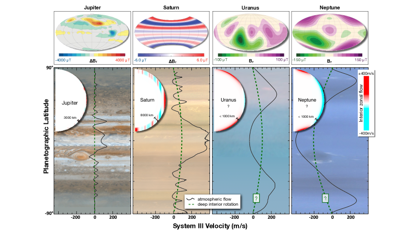
Figure 3: Magnetic fields, deep rotation, zonal winds and cloud bands on Jupiter and Saturn. The top panels show the non-dipole radial magnetic fields, for Jupiter at $0.9\rm\,R_{J}$ (from Moore et al., 2018), for Saturn at $0.75\rm\,R_{J}$ (from Dougherty et al., 2018), and the full radial fields for Uranus and Neptune at $1.0\rm\,R_{\rm tot}$ (from Soderlund and Stanley, 2020). Cloud bands, zonal winds, and deep rotation on the outer planets. The wind profiles are shown at the same scale for each planet and show zonal jets reaching 200-400 m/s; Jupiter and Saturn exhibit prograde equatorial jets, while Uranus and Neptune’s are retrograde. Deep rotation speeds (dashed lines) are determined from magnetic field rotation in Jupiter, seismology in Saturn (Mankovich et al., 2019), and estimated from planet shape arguments in Uranus and Neptune (Helled et al., 2010). Interior wind profiles (insets) are inferred from gravity data (Kaspi et al., 2018; Guillot et al., 2018). In Uranus and Neptune only an upper limit to zonal flow depth can be determined (Kaspi et al., 2013). Image credits: NASA/ ESA/ CICLOPS/ Bjorn Jonnson; winds from Porco et al. (2003), García-Melendo et al. (2011), Sromovsky et al. (2015), Karkoschka (2011) / T. Guillot, M. Hedman, L. Fletcher, A. Simon

The magnetic fields of giant planets all differ in surprising ways. Jupiter’s field is dipole-dominated with a $\sim 10^{\circ}$ tilt between the magnetic and rotation axis, with a non-dipolar part of the field which is confined almost entirely to the northern hemisphere and peaks at 3 mT, almost three times more than the peak dipolar field (Connerney et al., 2018; Moore et al., 2018). Saturn’s magnetic field is also dipole-dominated, with a nearly axisymmetric field, and a magnetic axis aligned with the spin axis to within $0.007^{\circ}$ (Dougherty et al., 2018; Cao et al., 2020). The fields of Uranus and Neptune are constrained only from flyby measurements by Voyager 2 in 1986 and 1989, respectively. They are highly multipolar, with a dipole component tilted by $59^{\circ}$ at Uranus and $47^{\circ}$ at Neptune (Soderlund and Stanley, 2020, and references therein).

The reason for Jupiter’s magnetic field strong north-south asymmetry (see Fig. 3) is not clear but it appears to preclude a dynamo operating in a thick, homogeneous shell. Rather, it has been proposed that this field morphology could arise from a dynamo operating in a thin layer, due to rapid variations in density or electrical conductivity (Dietrich and Jones, 2018; Moore et al., 2018). This again points to the presence of stably-stratified layers in the interior (Wicht and Gastine, 2020).

Saturn’s highly axisymmetrical field shown in Fig. 3 remains a mystery. A possibility is that the components of the fields are filtered out by a differentially-rotating stable conductive region above the dynamo region (Stevenson, 1982). Examination of the field measured by Cassini leads Cao et al. (2020) to estimate that this stable region must be at least 2500 km thick, i.e. 4% of Saturn’s radius. This seems incompatible with Saturn’s interior model as derived by Mankovich and Fuller (2021) which predicts a stable region at depth but none above the dynamo region.

Reproducing the complex yet weakly constrained multipolar magnetic fields of Uranus and Neptune is clearly a challenge, especially given the many unknowns on the planets’ interiors (see § 2.1). One possibility is that these fields result from thin-shell dynamos overlying a region of stable stratification, near $R/R_{\rm tot}\sim 0.7$ (Stanley and Bloxham, 2006). This would be qualitatively consistent with either the strong stratification due to a water-rich layer or the presence of a solid superionic shell around this location (Redmer et al., 2011, and § 2.1). But other possibilities are that the multipolar dynamos result from the planets’ relatively slow rotation rates and strong inertial effects (Soderlund et al., 2013) or from the complex interplay between moderate electrical conductivity and density stratification (Gastine et al., 2012).

Between the conducting interior where the dynamo originate and the atmosphere, rotation must change from being close to uniform (Cao and Stevenson, 2017) to being strongly dependent on latitude. As shown in Fig. 3, the gravity field measurements from Juno and Cassini enabled a determination of the depth of the transition region, at about 3000 km below the cloud tops ($R/\rm R_{J}\sim 0.96$) in Jupiter (Kaspi et al., 2018; Guillot et al., 2018) and about 8000 km ($R/\rm R_{S}\sim 0.86$) in Saturn (Iess et al., 2019; Galanti et al., 2019). The transition corresponds to an increase of hydrogen’s conductivity and may be attributed to magnetic field drag. In Jupiter, a secular variation of the magnetic field was detected and shown to be compatible with advection of the field by the zonal flow near 93-95% of the radius (Moore et al., 2019).

For Uranus and Neptune, the penetration depths of the winds are less constrained. Based on gravity data, the depths of the winds are estimated to be confined to a thin weather layer no more than $\sim$1,000 km ($\sim 96\%$ of the planetary radius) in both planets (Kaspi et al., 2013), consistent with estimates of the interior conductivity and Ohmic dissipation arguments (Soyuer et al., 2020). The rotation rate of their magnetic field, supposedly inferred from Voyager 2 data is also in question (Helled et al., 2010), with consequences for the interior structures of these planets (Nettelmann et al., 2013).

2.3 Atmospheres: Spatial & Temporal Variability

The atmospheres of giant planets represent the lens through which we glimpse the deep, hidden properties of the planetary bulk, and the transitional domain between the convective interior and the external charged-particle environment of the magnetosphere. As seen in Fig. 3 they are characterized by spatial variability, strong zonal winds and a remarkable banded structure. They also exhibit temporal variability on multiple timescales.

2.3.1 Banded Structure

Rotating fluid planets develop a system of planetary bands due to the dominance of the Coriolis force in the momentum balance, the injection of energy and momentum from small scales (eddies and storms) to larger scales (zonal jets), and the conservation of angular momentum and potential vorticity as differentially-heated air moves with latitude. These bands manifest in the ‘visible’ troposphere as a series of alternating prograde and retrograde zonal jets, separating bands of different temperatures, cloud opacity, and chemical composition. These contrasts are thought to be representative of vertical and meridional circulations on the scale of the bands, as we discuss below. The atmospheres accessible in our Solar System naturally fall into two categories:

• Rapid rotators ($\sim 10$ hours) with 5-8 bands in each hemisphere and a relatively uniform distribution of key condensables away from the equator (Jupiter and Saturn).

• Intermediate rotators ($\sim 17$ hours) with one equatorial retrograde jet, and a single prograde jet in each hemisphere, and strong equator-to-pole gradients in condensables (Uranus and Neptune).

These two groups are shown in Fig. 4, displaying their measured winds, tropospheric and stratospheric temperatures ($p<1$ bar, above the main clouds), and microwave brightness distributions. Microwave-dark regions exhibit significant absorption from condensing species (NH₃, H₂S, H₂O) in the few-tens-of-bars domain. Conversely, microwave-bright regions (e.g., at the poles of the ice giants) are depleted in volatiles. Hemispheric contrasts in temperatures and winds, driven by seasonal insolation and superimposed onto the smaller-scale banded structure, will be discussed in Section 2.3.3.

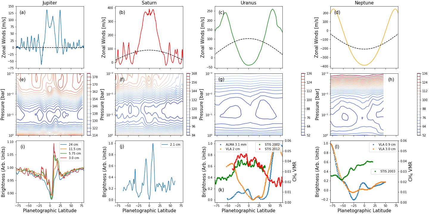
Figure 4: Latitudinal gradients in winds (top row), temperatures (middle row), and condensable volatiles (bottom row) for each of the giant planets. Cloud-tracked winds for (a) Jupiter in 2000 (Porco et al., 2003) and (b) Saturn in 2009 (García-Melendo et al., 2011) from Cassini; (c) Uranus from a combination of Voyager (1986) and Keck data in 2012-13 (Sromovsky et al., 2015), and (d) Neptune from Voyager in 1989 (Karkoschka, 2011). Tropospheric and stratospheric temperatures from Cassini/CIRS for (e) Jupiter in 2000 (Fletcher et al., 2016) and (f) Saturn between 2004-2009 (Fletcher et al., 2018), and from Voyager/IRIS for (g) Uranus in 1986 (Orton et al., 2015) and (h) Neptune in 1989 (Fletcher et al., 2014). Microwave brightnesses in the bottom row have been normalised for ease of comparison (for Jupiter, we normalise to latitudes beyond $20^{\circ}$). Microwave observations broadly sense NH₃ gradients for Jupiter (i) and Saturn (j); H$2$S gradients for Uranus (k) and Neptune (l). CH₄ does not condense and is well-mixed on Jupiter and Saturn (not shown); but condenses and displays latitudinal gradients on Uranus and Neptune (k, l). For (i) Jupiter, we show nadir brightness in four channels as measured by Juno in 2016-18 (Oyafuso et al., 2020). For (j) Saturn, we show 2.1 cm from passive radiometry with the Cassini radar 2009 (Laraia et al., 2013). For (k) Uranus, we show ALMA (2017) and VLA (2015) brightness scans from Molter et al. (2021), plus CH₄ from Sromovsky et al. (2014) from Hubble STIS observations (their Fig. 12, referenced to the right-hand axis); and for (l) Neptune, we show VLA (2015) brightness scans from Tollefson et al. (2021), alongside the CH₄ mole fraction estimated by multiplying the latitudinal gradients reported by Karkoschka and Tomasko (2011) from Hubble STIS observations (their Fig. 8) by the vertical profile in their Fig. 10, with a maximum deep mole fraction of 0.04. The mole fraction (referenced to the right-hand axis) should therefore be representative of abundances in the 1.8-3.0 bar region.

Fig. 4 demonstrates that giant planet atmospheres are latitudinally heterogeneous, with different latitudinal domains exhibiting somewhat different climatologies. A ‘classical’ picture of the bands of Jupiter and Saturn divides them into anticyclonic zones (with prograde jets on their poleward sides, retrograde jets on their equatorward sides) of low temperature, enhanced cloud opacity due to condensation, and enhanced abundances of species like NH₃, PH₃, para-H₂ due to upwelling (e.g., see reviews by Ingersoll et al., 2004; Del Genio et al., 2009). Conversely, cyclonic belts are regions of warmer temperatures, cloud-free conditions, and depletions in gaseous species. The implied temperature gradients are in geostrophic balance with the zonal winds, implying winds decaying with altitude from the cloud-tops into the stably-stratified upper troposphere and stratosphere (e.g., Conrath and Pirraglia, 1983). The belt/zone contrast is most apparent in the tropical regions in Fig. 4, featuring enhanced NH₃ and cool temperatures in the equatorial zones, and depleted NH₃ and warm temperatures in the equatorial belts (Gierasch et al., 1986; Achterberg et al., 2006; Janssen et al., 2013; Fletcher et al., 2016; Li et al., 2017). At mid-latitudes on Jupiter and Saturn, the correspondence between temperatures and winds remains clear, implying vertical decay of the winds, but the connection to gaseous abundances and aerosols becomes weaker (e.g., Fletcher et al., 2011; Giles et al., 2017; Antuñano et al., 2019; Grassi et al., 2020).

This picture of the banded structure was called into question by findings from the Galileo (Ingersoll et al., 2000), Juno (Fletcher et al., 2021), and Cassini missions (Fletcher et al., 2011). Several lines of evidence support deeper motions in the opposite sense to those described above (see Fletcher et al., 2020a, for a full review): lightning was found to be prevalent in Jupiter’s belts (suggesting uplift by moist convective plumes) (Ingersoll et al., 2000); eddy-momentum flux convergence into the zonal jets required a compensating meridional circulation with rising motion in belts, sinking in zones (Salyk et al., 2006; Del Genio and Barbara, 2012); and some chemical contrasts in Saturn’s deep troposphere appeared to oppose those seen in the upper troposphere (Fletcher et al., 2011). Adding to this, Jupiter’s microwave brightness gradients appear to flip in sign as we probe deeper into the atmosphere (Fletcher et al., 2021): belts are microwave-bright in the upper troposphere but microwave-dark below 5-10 bars (vice versa for zones). This could imply a series of stacked meridional circulation cells on the scale of the belts and zones, analogous to Earth’s Ferrel circulation cells (Duer et al. 2021, Fletcher et al. 2021, see also Ingersoll et al. 2017). The cells would be responsible for advecting NH₃ (and other gaseous species) in opposite directions above and below a transitional layer somewhere in the 1-10 bar region, creating ammonia-depleted belts at shallow depths, and ammonia-enriched belts at greater pressures.

Observations of Uranus and Neptune, from Voyager-2 in the 1980s, through three decades of ground- and space-based remote sensing, reveal atmospheres rather unlike the Gas Giants (e.g., see reviews by Mousis et al., 2018; Hueso and Sánchez-Lavega, 2019; Moses et al., 2020; Fletcher et al., 2020b). Fig. 4 reveals the same geostrophic balance between temperatures and winds, implying decay of the zonal winds with altitude (Conrath et al., 1998). Finer-scale albedo banding is observed on both planets, reminiscent of the bands of Saturn (e.g., Sromovsky et al., 2015), but to date no temperature or wind contrasts have been observed on these scales. However, the key difference from the Gas Giants is the strong equator-to-pole gradient in CH₄ (Karkoschka and Tomasko, 2011; Sromovsky et al., 2014) and H₂S (Molter et al., 2021; Takasao et al., 2021). The former manifests as bright poles in the visible and near-IR (due to the dearth of CH₄ absorption), the latter manifests as bright poles in the radio. These gradients may imply larger-scale circulation within and below the clouds, with air rising at the equator, moving polewards, and descending at high latitudes (de Pater et al., 2014; Sromovsky et al., 2014).

2.3.2 Deep Vertical Structure

We have few measurements of vertical structure in a planetary atmosphere below the 1 bar pressure level. In 1995, the Galileo probe plunged into Jupiter’s atmosphere with an entry speed of 47 km/s, at a 6.5^∘ North latitude, at the edge of a hot spot. The region was found to be relatively devoid of clouds (Ragent et al., 1998), with a relatively low abundance of condensates at higher levels: The abundance of NH₃ increased rapidly to $\sim 200$ ppmv near 2 bar and then slowly to its maximal value (between $400$ and $800$ ppmv) near 7 bar. That of H₂S increased progressively from $\sim 10$ ppmv near 9 bar to about 100 ppmv near 16 bar. Water was found to have a very low mixing ratio $\sim 50$ ppmv near 10 bar and reaching only $\sim 500$ ppmv near 20 bar, significantly less than the solar value (Wong et al., 2004). The probe also measured a temperature profile that was nearly dry adiabatic, except for regions with a static stability of $0.1$ to $0.2$ K/km at $0.5-1.7$ bar, $3-8.5$ bar, and $14-20$ bar (Magalhães et al., 2002). It reached a pressure of 22 bar for a temperature of 427.7 K.

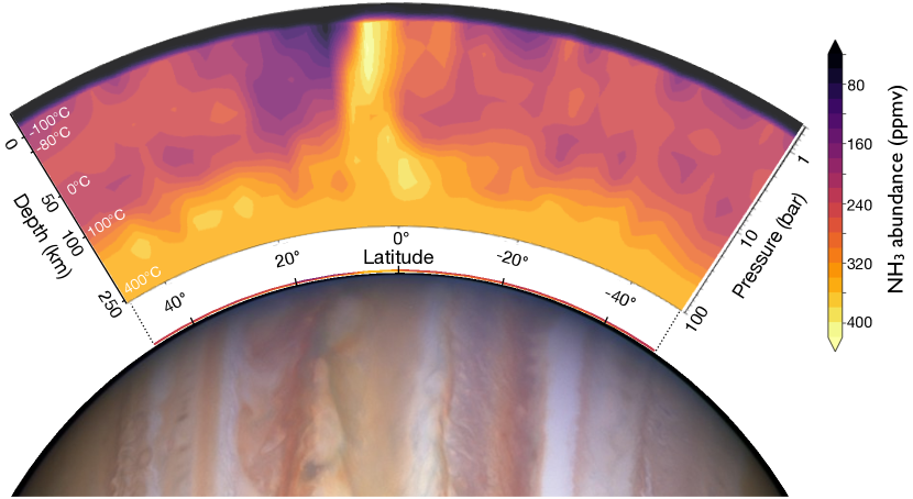
Figure 5: Ammonia abundance measured by Juno MWR in the deep atmosphere of Jupiter. The map corresponds to a mean abundance in parts per million by volume as a function of latitude and pressure level (or depth), obtained by a median average from 10 Juno flybys (PJ1 to PJ11) (from Li et al., 2017; Guillot et al., 2020b). The Jupiter visible image is from HST/WFC3/Mike Wong.

Ground-based observations from the Very Large Array have allowed probing Jupiter’s atmosphere, providing first evidence for a depletion of ammonia except near its equatorial zone (see de Pater et al., 2016, and references therein). But the Juno Microwave Instrument measurement, operating inside Jupiter’s synchrotron radiation belt at wavelengths of $3$ to $24$ cm (see Fig. 4) was able to probe the deep atmosphere, down to more than $100$ bar (Bolton et al., 2017a). As shown in Fig. 5, an inversion of the MWR data revealed that Jupiter’s ammonia has a variable abundance as a function of depth and latitude down to at least 200 km below the cloud tops, far beneath the expected cloud base (Li et al., 2017). The analysis of individual vortices also point to deep structures with variable depths, with both the microwave and gravity data showing that Jupiter’s Great Red Spot extends to about 300 to 500 km deep (Bolton et al., 2021; Parisi et al., 2021).

The ammonia depletion is correlated with enhanced lightning activity, as measured through the flash rate as a function of latitude (Brown et al., 2018). It has been proposed that during strong storms powered by water condensation in the $\sim 5$ bar region, ammonia vapor enables the melting of water ice crystal at very low temperatures $\sim-85^{\circ}$C, thus leading to the efficient formation of water-ammonia hailstones called mushballs (Guillot et al., 2020a). The downward transport of ammonia in stormy regions by mushballs and associated cold and dense downdrafts accounts for the Juno measurements (Guillot et al., 2020b). Importantly, the Juno results reveal that Jupiter’s deep atmosphere must be on average stable down to great depths. The abundance variations seen with ammonia could also apply to water, providing at least part of the explanation for the results of the Galileo probe. Finally, the same process at play on Jupiter should also apply to Saturn, Uranus and Neptune.

2.3.3 Temporal Variability

Two further sources of variability have not yet been discussed: changes to the atmosphere over time, and longitudinal variability associated with large-scale disturbances (vortices, plumes, waves, etc.). Indeed, long-term monitoring of the four giant planets reveals changes over timescales from years (seasons), to months (planet-wide disturbances), to days (storms), and even minutes (auroras and impacts). These phenomena could modulate light-curves seen from afar, so we discuss temporal variability in this section. On our journey through a giant planet from the inside out, this represents the top-most level that is most readily accessible to remote sensing: the upper troposphere and middle-atmosphere above the clouds, where reflected light and thermal emission in Fig. 6 can reveal dynamic and ephemeral phenomena.

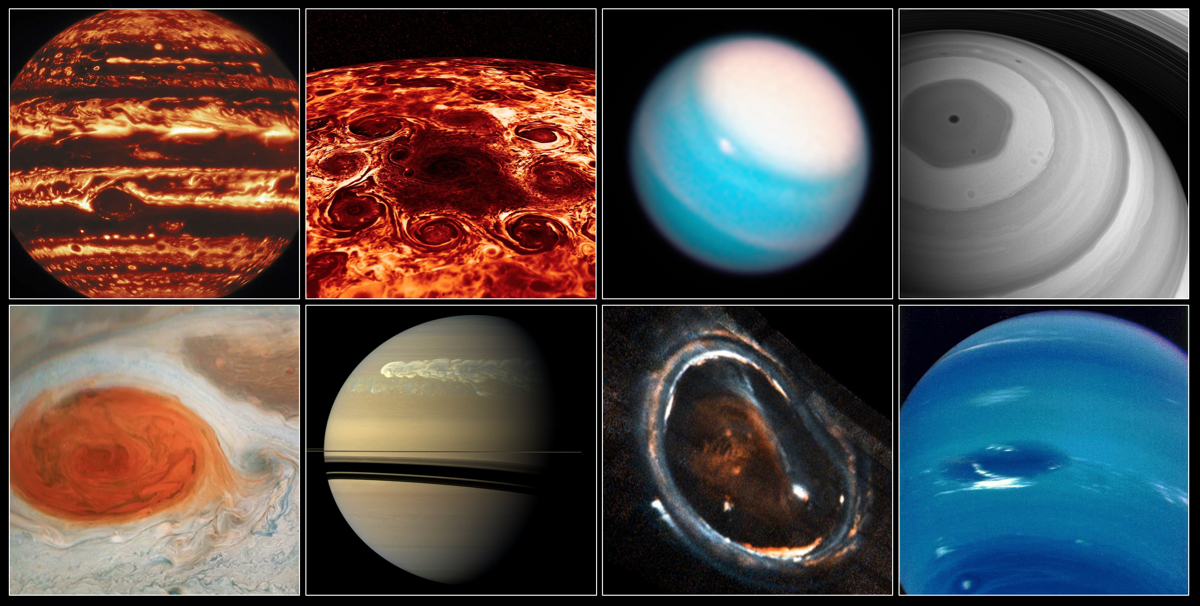
Figure 6: Examples of dynamic phenomena on the Giant Planets. Top row, left to right: Jupiter at 5 $\mu$m seen by Gemini (credit:Gemini Observatory/NOIRLab/NSF/AURA/M.H. Wong); and the north polar cyclone and ‘octagon’ of circumpolar cyclones observed at 5 $\mu$m by Juno (Adriani et al., 2018); Uranus’ seasonal reflective polar cap of aerosols observed by Hubble (credit:NASA/ESA/A. Simon/M.H. Wong/A. Hsu); and Saturn’s north polar hexagon and bands observed by Cassini (credit:NASA/JPL-Caltech/SSI). Bottom row, left to right: Jupiter’s Great Red Spot observed by JunoCam (credit: NASA/JPL-Caltech/SwRI/MSSS/Gerald Eichstädt/Seán Doran); Saturn’s 2010-11 storm system from Cassini (credit:NASA/JPL-Caltech/SSI); Jupiter’s north polar auroral oval observed in the UV by Juno (Mauk et al., 2017); and Neptune and its Great Dark Spot observed by Voyager 2 (credit:NASA/JPL-Caltech).

Absorption of short-wave sunlight by methane and aerosols dominates radiative heating, to be balanced by thermal emission and radiative cooling by the collision-induced hydrogen-helium continuum, and from stratospheric acetylene (13 $\mu$m), ethane (12 $\mu$m), and to a lesser extent methane (7 $\mu$m). Planets with Earth-like axial tilts (Saturn and Neptune), or extreme obliquities (Uranus), might therefore be expected to display seasonal variability. The radiative time constant characterises an atmosphere’s inertia to temperature response to seasonal change - this is shortest in the upper and middle-atmosphere, but lengthens at higher pressures so that temperatures in the troposphere tend to follow the annual-averaged insolation. Observations of the upper troposphere and stratospheres, however, tend to see seasonal asymmetries in temperatures, stratospheric chemicals (from a combination of temperature- and sunlight-dependent reactions and seasonally-dependent vertical mixing), and aerosols/hazes (from seasonally-dependent growth of aerosols). The former has been revealed via 13 years or orbital remote sensing of Saturn by the Cassini spacecraft, whereas the latter is exemplified by the slow seasonal growth of tropospheric aerosols at the Uranian poles, producing reflective polar caps (Sromovsky et al., 2019). These slow seasonal variations can also be influenced by periodic variations on shorter timescales, such as those associated with equatorial stratospheric oscillations on Jupiter (Leovy et al., 1991) and Saturn (Fouchet et al., 2008; Orton et al., 2008), or those associated with seasonally-reversing stratospheric circulations (e.g., Friedson and Moses, 2012). Thus any disc-averaged observations sensing domains in the radiatively-controlled middle atmosphere could find conditions biased towards particular seasons or phases of seasonally-dependent phenomena.

Besides the seasons, planetary emission and reflection are observed to vary over shorter, but still periodic, cycles. Entire bands of Jupiter can be seen to fade (i.e., whiten over) and then spectacularly revive (i.e., regain their red-brown colour) due to localised convective plumes (Fletcher et al., 2017). Other bands expand and contract in latitude with predictable, but poorly understood timescales (Antuñano et al., 2019), although the influence of these changes on light curves may be minimal (Ge et al., 2019). The brightness of Uranus and Neptune has been monitored over many decades (Lockwood, 2019), appearing to show some relationship with the solar cycle (Aplin and Harrison, 2016), exemplifying planet-star interactions as a driver for the brightness of an atmosphere. Saturn’s 2010 storm is an extreme example of a storm modulating temperature and composition variations with longitude and time (Sanchez-Lavega et al., 2018), creating a new cloud-free and volatile-depleted band that persisted for many years after the storm, and producing huge changes to stratospheric temperatures and chemistry known as the ‘beacon’ (Fletcher et al., 2012). These storms appear to occur on seasonal timescales, potentially as a result of a radiatively influenced charge-recharge cycle associated with the overcoming of convective inhibition near the water-cloud (Li and Ingersoll, 2015).

Water is key to understanding the giant planets, playing a crucial role in their meteorology. Moist convection may be the most important mode of transport for internal heat on Jupiter and Saturn (Gierasch et al., 2000), although water storms are observed to be highly intermittent, localised, but widespread (Hueso et al., 2002; Sugiyama et al., 2014; Brown et al., 2018). In the case of Jupiter’s planet-wide disturbances, immense clusters of water-driven plumes are readily visible and reflective in certain longitude domains. Disturbances in Jupiter’s North Temperate Belt generate vigorous plumes within a few days of one another, but at widely separated longitudes, indicating some degree of connection over many thousands of kilometres (e.g., Sánchez-Lavega et al., 2008). Like Saturn’s storm, these sporadic water plumes could create ephemeral changes to a rotational light curve, whilst associated precipitation could also transport condensed volatiles down to great depths (Guillot et al., 2020a, b). Understanding the occurrence of these storms remains a significant challenge, given the stabilising effects of the molecular weight of moist air (i.e., convective inhibition), balanced by the buoyant effects of latent heat release (Guillot, 1995; Leconte et al., 2017). Unfortunately, the depth of this water-driven convection is hard to access on Jupiter and Saturn, but methane-driven convection on the Ice Giants may provide a vital means for testing convection in hydrogen-rich planets at higher, more accessible altitudes (Hueso et al., 2020).

Periodic variations in planetary atmospheres, in addition to sporadic storms, will cause a planet’s disc-averaged emission to change with time. In addition, giant planet atmospheres host vortices with a variety of scales (e.g., Ingersoll et al., 2004; Vasavada and Showman, 2005), from large-scale anticyclones (typically cool and cloudy with white or red aerosols on Jupiter and Saturn, or darker ovals on Uranus and Neptune with their associated ‘orographic’ white clouds), to smaller scale and often elongates cyclonic structures (typically cloud-free but prone to outbursts of convection creating turbulent filamentary patterns). Small vortices are unlikely to be accessible in the disc-average, but the largest anticyclones (Jupiter’s Great Red Spot and Neptune’s Great Dark Spot) could modulate the light curve at the rotation period. Indeed, rapidly-evolving storm features on Neptune were seen to modulate the lightcurve measured by Kepler as the planet rotated (Simon et al., 2016). These vortices evolve with time, such as the shrinking of Jupiter’s Great Red Spot (Simon et al., 2018), or the equatorward drifting and eventual disappearance of Neptune’s Great Dark Spot (Stratman et al., 2001).

Finally, giant planet atmospheres are influenced by external processes, including cometary impacts and interplanetary dust (Moses and Poppe, 2017), and auroral heating (O’Donoghue et al., 2021). Fig. 6 shows an example of UV emission from Jupiter’s northern aurora, where energy injection is known to heat the thermosphere and ionosphere to significantly higher temperatures than would be expected from solar heating alone.

2.3.4 Implications for the Characterisation of Exoplanets

With the caveat that the environmental conditions encountered on the present-day census of exoplanets and brown dwarfs will be significantly different to our own giant planets , the discussion above suggests latitudinal and vertical variability could influence the interpretation of disc-averaged observations: (i) Certain latitude domains will be significantly brighter in the thermal than colder, cloudier, volatile-enriched regions - the belts of Gas Giants, or the poles of Ice Giants. These brighter domains may contribute more to the disc average, meaning a bias towards volatile-depleted and cloud-free regions. An extreme case is Jupiter at 5 $\mu$m, where radiance is only observed from cloud-free belts and compact features, like Galileo’s infamous ‘hotspot.’ Furthermore, if a giant exoplanet is viewed from an oblique angle (e.g., consider the appearance of Uranus as it approaches solstices), a volatile-depleted polar domain may dominate the disc average. (ii) The ‘climate domain’ being characterised depends on the depth of penetration at the wavelength of interest - observations sounding the deeper troposphere would reveal conditions rather different to those sensing the upper troposphere (or even the stratosphere, see § 2.3.3). It is also clear that cloud condensation sometimes deviates from the equilibrium expectations: aerosol layers rarely occur where they are expected, and deep volatiles show considerable spatial variability and vertical gradients, rather than being well-mixed. Put simply: vertically-layered climate domains with different compositions and circulations are likely adding complexity to interpretation of disc-averaged spectra.

In summary, inferring the properties of the deep interior and bulk composition ‘from the outside in,’ when it is hidden beneath such a highly variable and complex atmospheric layer, should remain a significant challenge for any giant planets.

2.4 Composition

2.4.1 Bulk composition

The bulk chemical composition of each planet reflects the proportion of rocks, ices, and gases accreted by the forming giants from the surrounding nebula (see § 4 hereafter). Unfortunately, we presently cannot distinguish between rocks and ices, something that would be highly desirable in order to constrain the history of the formation of the solar system (see Kunitomo et al., 2018). Instead, we have to treat them together as heavy elements.

Jupiter is the planet for which the uncertainties on interior composition have been the largest, owing mostly to the fact that a large fraction of its interior lies in this 0.1 to 10 Mbar region for which the EOSs of hydrogen and helium are the most uncertain (see § 2.1.2). Three-layer models inferred a total mass of heavy elements between $10$ and $42\rm\,M_{\oplus}$ for a core smaller than about $10\rm\,M_{\oplus}$ (Saumon and Guillot, 2004). Recent models based on the Juno measurements (§ 2.1.4) have not narrowed down this uncertainty, with a total mass of heavy elements ranging from about 8 to $46\rm\,M_{\oplus}$ (Wahl et al., 2017a; Debras and Chabrier, 2019; Ni, 2019; Nettelmann et al., 2021; Miguel et al., 2022). The central compact core is smaller than $7\rm\,M_{\oplus}$ (Miguel et al., 2022), with most of the heavy element mass being held in a dilute core that may encompass a limited region to most of the metallic hydrogen envelope (see Fig. 1). Most of these uncertainties are linked to uncertainties in the equations of state of hydrogen and helium (e.g. Mazevet et al., 2020). In addition, a significant tension exists between interior models which favor low metallicities for the outer envelope, in contradiction with atmospheric constraints. Possible solutions include a heavy element abundance that would decrease with depth in the molecular envelope region (Debras and Chabrier, 2019) or higher temperatures in the deep atmosphere (Nettelmann et al., 2021; Miguel et al., 2022), both raising further questions in terms of the long-term stability and formation of such an inverted Z-gradient and in terms of possible latitudinal temperature variations in Jupiter, given the Galileo probe constraint.

On Saturn, three-layer models were predicting a total mass of heavy elements between $16$ and $30\rm\,M_{\oplus}$ and a compact core mass between $8$ to $25\rm\,M_{\oplus}$ (Saumon and Guillot, 2004). The gravitational and seismological constaints from Cassini allow Mankovich and Fuller (2021) to derive much tighter constraints, a total mass of heavy elements $19.1\pm 1.0\rm\,M_{\oplus}$ and a compact+dilute core containing $17.4\pm 1.2\rm\,M_{\oplus}$ of rocks and ices. Interestingly, the amount of rocks and ices in the envelope is relatively limited corresponding to an envelope metallicity $Z_{\rm out}=0.041\pm 0.009$. Again, as for Jupiter, this may be in tension with the generally high metallicity of Saturn’s atmosphere (§ 2.4.2).

Unfortunately, the lack of accurate constraints on Uranus and Neptune’s gravity fields translates into considerable uncertainties for these planets, with in particular the impossibility to determine whether they are formed of discrete layers (as in Fig. 1) or instead mixed regions with progressive compositional gradients. Interior models suggest a metallicity of $\sim 76\%$ to 90% for Uranus and 77% to 90% for Neptune (Helled et al., 2011; Nettelmann et al., 2013). While they are called ”ice giants”, we presently have no information on their rock-to-ice ratio (Helled et al., 2020a).

2.4.2 Atmospheric Composition

The extent to which the observed atmospheric composition (from the stratosphere to the deeper troposphere at a few tens of bars) reflects that of the deeper interior remains an open question. Atmospheric remote sensing, in addition to in situ measurements by the Galileo probe, reveal that cosmogonically-common elements are present in their reduced/hydrogenated forms, either as condensable volatiles (methane, ammonia, H₂S, water), disequilibrium tracers (e.g., PH₃, AsH₃, GeH₄, CO), photochemical products of UV photolysis (e.g., tropospheric hazes, stratospheric hydrocarbons), or as externally-sourced contaminants to the upper atmosphere. The elemental abundances measured on each planet is provided in Table 2, and shown in Fig. 7. However, as the vertical distribution of each molecular species can influenced by chemical sinks (condensation, photochemistry) and sources (e.g., vertical mixing), accessing well-mixed ‘bulk’ reservoirs is a distinct challenge.

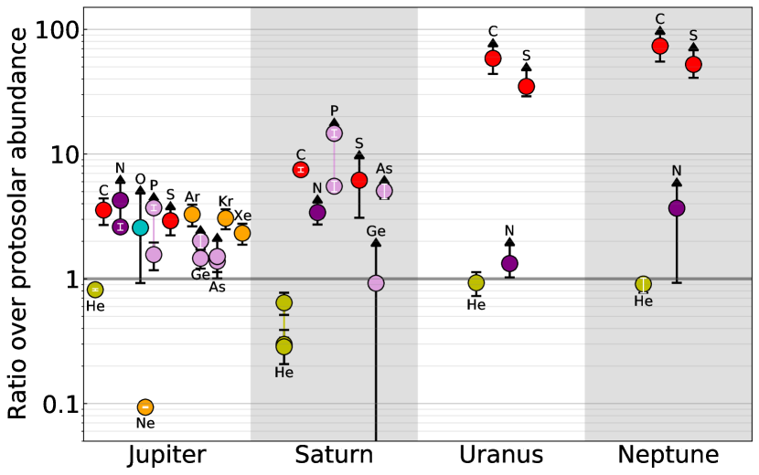
Figure 7: Elemental abundances of He, C, N, O, P, S, Ar, Ge, As, Kr and Xe in protosolar units in Jupiter, Saturn, Uranus and Neptune. Elements carried by chemical species which are condensing in the atmosphere (e.g., C, which is mainly carried as CH₄ which condenses in Uranus and Neptune) are indicated by a top arrow. For these species, when the abundance is variable (horizontally and vertically), the maximum value was chosen. Several points are sometimes provided for a given species when several measurements are available. The colours are green for helium, orange of noble gases, red for carbon and sulfur, purple for nitrogen, blue for oxygen and pink for elements carried by disequilibrium species. See Table 2 for values.

Classical thermochemical ‘equilibrium’ models predict the formation of condensate clouds from key species (methane, ammonia, hydrogen sulphide, water) in relatively well-defined layers, and uniform mixing below (Atreya et al., 2003). For the top-most clouds on the Gas Giants (NH₃ ice and solid NH₄SH), Cassini and Juno measurements of the abundances of NH₃ (Laraia et al., 2013; Fletcher et al., 2011; de Pater et al., 2016; Li et al., 2017) below the clouds has shown to be highly variable, and even less is known about H₂S, with estimates of elemental abundances being subject to considerable uncertainty owing to (i) remote-sensing degeneracies between abundance, temperature, and aerosols; and (ii) spatial variability associated with dynamics and meteorology. The latter implies that it remains unclear how representative the Galileo in situ measurements were for Jupiter’s atmosphere. The top-most clouds of the Ice Giants (CH₄ ice and H₂S ice) also limit the accessibility of the bulk carbon and sulphur enrichments: estimates of CH₄ and H₂S rely on precise separation of gaseous absorption from cloud reflectance in the near-infrared (Karkoschka and Tomasko, 2009, 2011; Sromovsky et al., 2014; Irwin et al., 2018), or on millimetre-centimetre-wave sounding (Molter et al., 2021; Tollefson et al., 2021), both of which are further hindered by strong equator-to-pole gradients in condensables (see §2.3.1). Only methane on the Gas Giants has been reliably constrained as temperatures are too warm for condensation and, in the absence of carbon sinks, the derived CH₄ is expected to be representative of the bulk (Wong et al., 2004; Fletcher et al., 2009a).

In summary, extrapolating atmospheric abundances of condensibles (and disequilibrium species) to the deeper interior is fraught with difficulty, and this is before we reach a vitally-important molecule for understanding planet formation: water. The importance of water ice as a carrier of elements to forming planets means that it remains an essential comparative measurement on all four giants. On Uranus and Neptune, it is locked away at such great depths that we can only infer its abundance indirectly by means of its chemical reactions with measured disequilibrium species like CO, after having separated stratospheric CO (which can arise from external sources, such as cometary impacts or interplanetary dust, Bézard et al., 2002) from the tropospheric reservoir. (Cavalié et al., 2017; Venot et al., 2020; Moses et al., 2020) derive an upper limit to the O/H ratio of 250 times solar in Uranus and a value between 250 and 650 times solar in Neptune, but these values are highly uncertain due to our poor understanding of CO transport. On Jupiter and Saturn the well-mixed water could be shallower and more readily accessible, but infrared spectral signatures of H₂O are only seen over limited domains and oft associated with vigorous dynamics (Sromovsky et al., 2013; Bjoraker et al., 2018; Grassi et al., 2020). Hopes to derive Jupiter’s bulk water abundance via the Galileo probe were dashed when it entered a dry and desiccated region near the equator (known as a 5-$\mu$m hotspot, Orton et al., 1998), where water was found to be significantly sub-solar and still increasing at 20 bars (Wong et al., 2004). Juno’s Microwave Radiometer (Bolton et al., 2017a) is capable of measuring water at tens of bars, provided its opacity can be disentangled from the horizontally- and vertically-variable distribution of NH₃ (Li et al., 2017), something which has only been accomplished at the equator so far (Li et al., 2020), where it is at least solar in abundance near its 6-bar condensation level. Determinations of giant planet bulk-water content remains an active area of research.

Despite the challenges associated with many of the species in Table 2, we note that the noble gases are chemically inert, meaning that the Galileo probe measurements (Atreya et al., 2003; Wong et al., 2004) are expected to be representative of Jupiter’s bulk. A notable exception is neon, predicted to dissolve into helium-rich droplets inside Jupiter and Saturn (Roulston and Stevenson, 1995; Wilson and Militzer, 2010) and indeed depleted in Jupiter (Wong et al., 2004). Unfortunately, the absence of in situ measurements for any other giant planet hampers attempts at comparative planetology, so noble gas measurements should be a key goal for future giant planet exploration. Finally, we note that comparisons of isotope ratios (see Table 3) in common molecules provides further constraint on planetary accretion. These are discussed in § 4.3.3 hereafter.

3 CHARACTERIZING BROWN DWARFS AND GIANT EXOPLANETS

Currently, thousands of brown dwarfs (Best et al., 2018) and nearly a thousand exoplanets (Thompson et al., 2018) are known. The boundaries between brown dwarfs, self-luminous directly imaged young planets, and close-in transiting planets are mostly artificial as these objects occupy a continuum in irradiation ($0$ to $10^{4}$ that of the Earth), mass (M_⊕ to $\sim 80$ M_jup), rotation periods (hours to days), internal heat flux (none up to 1000s of K), and composition (solar to $\sim$100s $\times$ solar). Understanding these atmospheres is key to understanding this continuum and providing clues as to their possible formation avenues. Most of the focus to date has been on determining the abundances of the major carbon, oxygen, and nitrogen bearing species as well as metals like iron, magnesium, and the alkali’s, both because these were the most easily observable with the current instruments and because they are thought to be the primary “heavy element” tracers of planet formation (see §4). Below we summarise how we obtain abundance information from the these objects and how we can leverage abundances across this diverse population to provide insight into planet formation processes.

3.1 Constraining Interior Structure & Composition

3.1.1 Evolution Models

As seen in Fig. 2, giant planets and brown dwarfs cover a range of pressures and temperature in which hydrogen is fluid and therefore, compressible. After a first phase of accretion and rapid contraction in which their interior heats up, their contraction continues through a cooling of the interior. For a planet like Jupiter, about half of the planet’s gravitational potential energy corresponds to the intrinsic luminosity and is radiated away. This loss also corresponds to a decrease of the thermal energy of the protons. However, the planet’s internal energy still increases as it should because the energy of the degenerate electron gas increases by a larger amount (Guillot, 2005). For ice giants, coulombian effects and phase changes imply that the compressibility is reduced, but still significant.

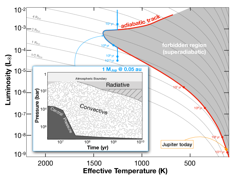
Figure 8: Theoretical Hertzprung-Russell diagram for a $1\rm\,M_{Jup}$ planet in isolation (red) and at 0.05 au from a solar-type star (blue) (from Guillot et al., 1996). The effective temperature corresponds to the sum of the planet’s intrinsic and absorbed stellar flux. Evolution times are indicated in years (from $10^{7}$ to $10^{10}\,$yr after an arbitrary initial condition). Dotted curves indicate planetary radius. Inset: Kippenhahn diagram (see Kippenhahn and Weigert, 1990) showing the evolution of the interior structure of the $1\rm\,M_{Jup}$ at 0.05 au from its star and the growth of the inner radiative zone (from Guillot and Showman, 2002). The radiative-convective zone boundary may be limited because of heat dissipation, in which case the hashed region should remain convective. Alternatively, the radiative zone may be extended but less statically stable due to wind-driven downward energy advection (see text).

In this regime, the opacities are high, the release of primordial heat due to the loss of internal entropy is progressive, implying that, in isolation, substellar objects are fully convective (Burrows et al., 1997; Baraffe et al., 1998). But irradiation effects can alter this picture: When the intrinsic luminosity becomes of the same order or smaller than the irradiation luminosity, as shown in Fig. 8, a radiative zone must develop below the photosphere in order to allow the planetary interior to continue to cool (Guillot et al., 1996).

Given an approximate age, and a measurement of the mass and radius, given appropriate evolution models, it is therefore possible in principle to provide constraints on the bulk composition of giant planets and brown dwarfs. Cooling tracks for these objects (e.g., Fortney et al., 2007) are essentially defined by the EOSs, atmospheric properties, and radiative opacities. The presence of a central heavy element core leads to a planet being smaller compared to the same planet without a core. Enriching the envelope uniformly however leads to opposing effects: On one hand, the increase in mean molecular weight tends to increase the planetary density. On the other hand, this is opposed by an increase in the opacity in the radiative zone which slows the cooling. It also leads to a slightly change in atmospheric properties. Models show that for highly irradiated planets, the opacity effect dominates at early times, in the first Gyr or so, and then at later times, molecular weight effects begin to dominate (Guillot, 2005; Baraffe et al., 2008).

An outstanding issue however is that a significant fraction of known hot-Jupiters (i.e., with orbital periods closer than about 10 days around solar-type stars) are oversized compared to theoretical predictions (Bodenheimer et al., 2001; Guillot and Showman, 2002). Many possibilities have been proposed to solve this, including, tides (Bodenheimer et al., 2001), downward kinetic energy transport (Guillot and Showman, 2002), convective inhibition (Chabrier and Baraffe, 2007), enhanced atmospheric opacities (Burrows et al., 2007), thermal tides (Arras and Socrates, 2010), ohmic dissipation (Batygin and Stevenson, 2010) or wind-driven downward advection of energy (Youdin and Mitchell, 2010; Tremblin et al., 2017). Statistical studies show that the effect is more pronounced for planets with equilibrium temperatures around $T_{\rm eq}\sim$2000 K (Thorngren and Fortney, 2018; Sarkis et al., 2021). This dependence on equilibrium temperature rules out tides, convective inhibition, and enhanced opacities, favouring instead mechanisms that tap of order $\epsilon\sim 1\%$ energy from the stellar irradiation reservoir (see Guillot and Showman, 2002). The fact that models with $\epsilon$ increasing from $\sim$0 for $T_{\rm eq}\sim 1000$ K to $\sim$3% for $T_{\rm eq}\sim 1500-2000$ K and decreasing past that value are strongly favoured statistically (Thorngren and Fortney, 2018; Sarkis et al., 2021) points to the importance of magnetic drag that leads to slower atmospheric winds on highly irradiated planets (Perna et al., 2010; Menou, 2012; Ginzburg and Sari, 2016). Thus, mechanisms involving Ohmic dissipation (Batygin and Stevenson, 2010), wind-driven downward advection of energy (Youdin and Mitchell, 2010; Tremblin et al., 2017; Sainsbury-Martinez et al., 2019) or thermal tides (Arras and Socrates, 2010) appear favoured.

The downward energy transport that results has consequences for the extent and structure of the interior radiative zone in hot-Jupiters. While standard models predict it to grow to reach $\sim$kbar levels in a few Gyr (see Fig. 8), evolution models aimed at reproducing observable constraints imply that the extent of this radiative zone should be limited to a few hundred bars for $T_{\rm eq}\lesssim 1000$ K to a few bars for $T\gtrsim 2000$ K (Thorngren et al., 2019; Sarkis et al., 2021). However, for wind-driven downward energy advection, the entire temperature profile of the radiative region would be affected (Tremblin et al., 2017), with the possibility of a smaller static stability but deeper radiative-convective boundary than for a heat deposition at greater depth.

For temperate giant planets, the most important effects to be considered in light of the new developments for solar system planets are (1) changes to the atmospheric structure and (2) consequences of possible compositional gradients. As seen from Fig. 2, phase changes in the deep interior should affect only a small fraction of the known population of giant exoplanets, those with relatively small masses and low irradiation temperatures. However, the condensation of elements should be taken into account, particularly for objects with effective temperatures below 375 K which begin condensing water (Morley et al., 2014). Finally, deep compositional gradients are acting in two ways: By suppressing convection, they can store heat and release it at a later time (e.g. Chabrier and Baraffe, 2007; Leconte and Chabrier, 2012). By leading to upward mixing (core erosion) they also affect the energy balance (Guillot et al., 2004; Moll et al., 2017). These effects can potentially modify the planetary evolution, something that is still to be examined.

3.1.2 Inferring Bulk Abundances

Given an evolution model, the total (bulk) amount of heavy elements in a giant planet or a brown dwarf can be inferred from the knowledge of its age, mass, and either radius or luminosity. In practice, measurements of luminosities can only be made for brown dwarfs and bright planets which therefore must be massive and/or young. In these cases, such constraint is presently very difficult to obtain becasue of the small relative mass of a potential core, the uncertainties on the initial entropy and/or on the atmospheric properties.

Transiting planets have therefore been the target of choice to obtain bulk metallicities. For simplification purposes, models have usually assumed that heavy elements are entirely embedded into a central dense core (see § 3.1.1 for details). The technique was first applied to hot Jupiters, by arbitrarily transporting a fraction $\sim 1$% of the irradiated energy to the planetary interior in order to account for the inflation problem (Guillot et al., 2006). This assumption however can be lifted by limiting the ensemble to the cooler transiting planets for which the inflation mechanism becomes negligible (Thorngren et al., 2016). The results consistently highlight a great diversity of bulk compositions, with planets which can have very low to very high masses in heavy elements (e.g., Guillot et al., 2006; Burrows et al., 2007; Moutou et al., 2013; Thorngren et al., 2016). Whereas a correlation between the heavy element content of planets and the metallicity of their host star was found for hot Jupiters (Guillot et al., 2006; Moutou et al., 2013), it was not confirmed in a sample of 24 well-characterized warm Jupiters (Teske et al., 2019).

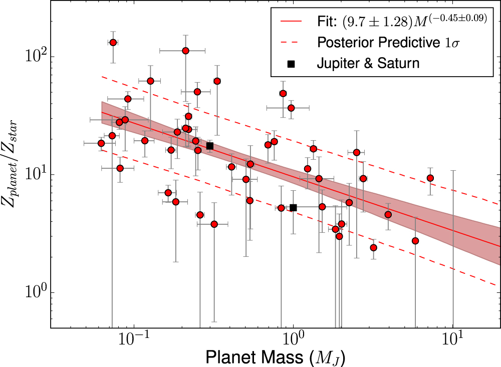
Figure 9: Heavy element enrichment of non-inflated transiting planets relative to their parent stars as a function of mass. The line is the median fit to the distribution from bootstrapping, with 1, 2, and $3\sigma$ error contours. Jupiter and Saturn are shown in blue, from Guillot (1999). [From Thorngren et al. (2016)]

A robust inverse correlation shown in Fig. 9 links the giant planets heavy element content and their mass (Thorngren et al., 2016). This inverse relation, expected in the framework of core-accretion formation models, indicates a bulk enrichment of $\sim 30$ for $0.1\rm\,M_{Jup}$ planets decreasing to $\sim 3$ for $10\rm\,M_{Jup}$ planets. It is important to caution that the spread in that relation is very large: In Fig. 9, some $0.1\rm\,M_{Jup}$ planets end up much less enriched than some $\sim 1\rm\,M_{Jup}$ planets. While massive planets tend to be relatively less heavy-element rich than their lighter counterparts, the dominant feature remains the very large diversity of bulk properties for any given planetary mass.

3.1.3 Towards Exoplanetary Core Masses

In very special circumstances, one can obtain a constraint on the interior structure of an exoplanet. This is the case when the Love number of a planet, i.e., the proportionality relation between an applied tidal potential and the induced field at the surface of the planet, can be measured through its apsidal precession (Ragozzine and Wolf, 2009). This link requires a system of two planets orbiting a central star in a so-called fixed-point eccentricy configuration. Batygin et al. (2009) and Mardling (2010) show that the second Love number $k_{2}$ of the inner planet can be determined if (i) the mass of the inner planet is much smaller than the mass of the central body, (ii) the semimajor axis of the inner planet is much less than the semimajor axis of the outer planet, (iii) the eccentricity of the inner planet is much less than the eccentricity of the outer planet, (iv) the planet is transiting, and (v) the planet is sufficiently close to its host star, such that the tidal precession is significant compared to the precession induced by relativistic effects (Buhler et al., 2016).

The HAT-P-13 system is the first and only currently known system to fulfill these criteria. It consists of a central $1.3\rm\,M_{\odot}$ G-type star, and two planets, HAT-P-13 b with a mass of $0.9\rm\,M_{Jup}$, a radius of $1.5\rm\,R_{Jup}$ and an orbital period of 2.91 days, and the outer HAT-P-13 c which has a minimum mass of $14.2\rm\,M_{Jup}$, an orbital period of 446 days and an eccentricity of 0.66 (Bakos et al., 2009; Winn et al., 2010; Southworth et al., 2012). An outer massive companion lies between 12 and 200 au (Winn et al., 2010). Observations of secondary eclipses of HAT-P-13 b lead to an eccentricity $e_{\rm b}=0.007\pm 0.001$, a value of the Love number $k_{2}=0.31_{-0.05}^{+0.08}$ leading to a core mass that is $<25\rm\,M_{\oplus}$ (68% confidence interval) (Buhler et al., 2016). For comparison, on Jupiter, gravity fields measurements indicate a Love number associated with Io’s tide $k_{22}=0.565\pm 0.006$ (Durante et al., 2020), slightly lower than static model predictions (Wahl et al., 2016), but in agreement with theory when accounting for the Coriolis acceleration (Idini and Stevenson, 2021). In Saturn, astrometric constraints indicate that $k_{2}=0.390\pm 0.024$ (Lainey et al., 2017), in line with model predictions (Wahl et al., 2017b).

The possibility to measure core masses is extremely interesting. The difficulty with the fixed-point eccentricity configuration is that it is rare and an extremely accurate determination of the eccentricity of the inner planet is needed. Future determinations may rely instead on extremely accurate ($<50$ ppm/min photometric precision) determination of planetary shape (see Akinsanmi et al., 2019). This method is possible with space-based photometry only, but is not limited to systems in a fixed-point eccentricity configuration.

3.2 Atmospheric Abundances from Spectra

Classic stellar spectroscopy involves measurements of the self-luminous thermal emission from an isolated (field) star. Equivalent-width analyses or data-model spectral synthesis tools are used to extract precise constraints ($<$0.1 dex) on elemental abundances while accounting for uncertainties in the stellar effective temperature and gravity (Asplund, 2005). Like stars, spectroscopic characterisation (Figure 10) is the primary tool by which we can answer fundamental questions regarding the intrinsic composition of these objects and their possible formation history (Madhusudhan, 2019; Kirkpatrick, 2005). However, most sub-stellar objects are typically of temperatures much lower than stars ($<$3000K)–abundance analyses must leverage both atomic and molecular opacity sources–classic stellar abundance analyses cannot be used.

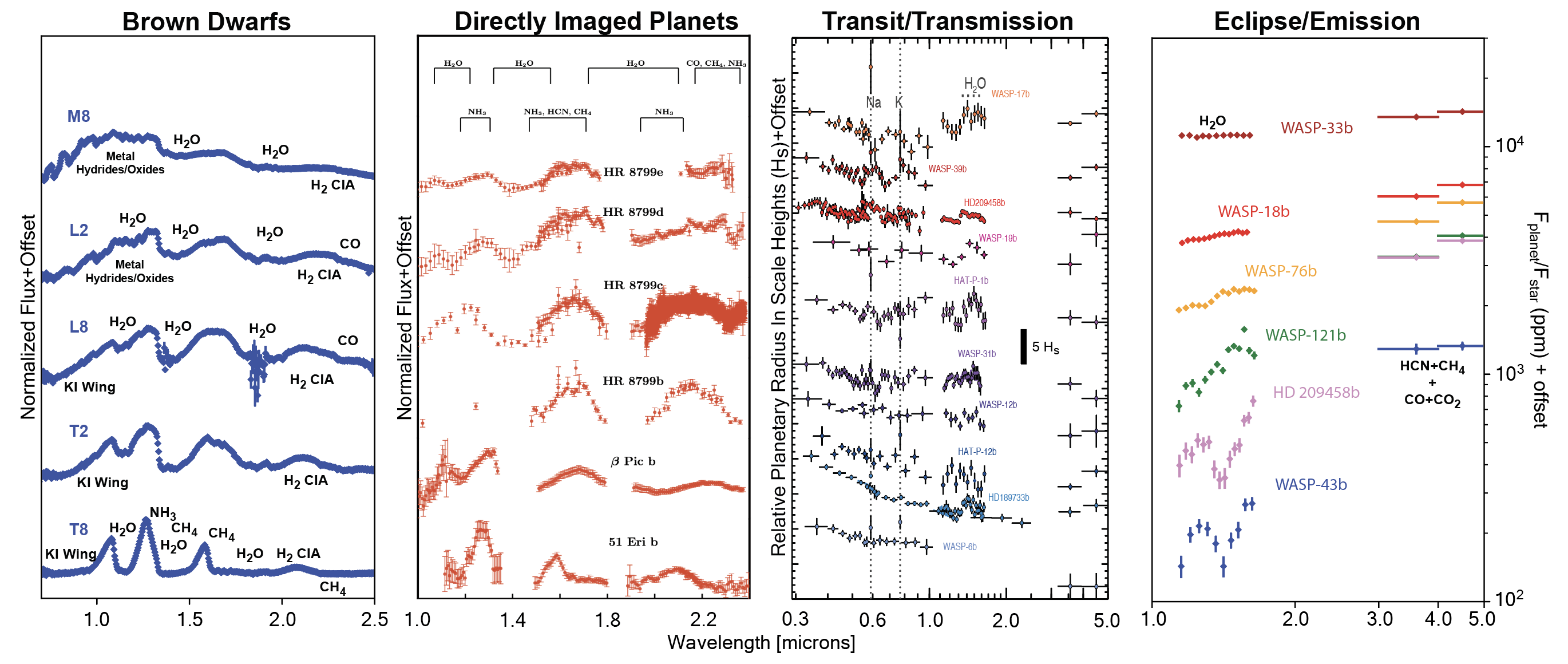
Figure 10: Summary of typical spectra obtained, from left to right, for brown dwarfs (from the SpeX Prism Library), directly imaged self-luminous exoplanets (from Madhusudhan (2019)), and transiting planets in transmission (from Sing et al., 2016) and in eclipse/thermal emission (Mansfield et al., 2021). The spectra of all objects are carved out by various atoms, molecules, and grain opacity. We can leverage these opacity sources to extract meaningful abundance information like atmospheric metal enrichment and elemental abundance ratios.

Instead, model dependent parameter estimation methods (“atmospheric retrievals”) are employed to extract the pertinent, often degenerate, information. These entail a forward model that takes in as parameters the vertical temperature-pressure profile, numerous abundance parameters, and any other nuisance/process parameters. This forward model is combined with a parameter estimator, like Markov chain Monte Carlo (see Madhusudhan (2018) for a review of retrieval methods) to fit the data and to find the optimal parameters and corresponding uncertainties. The resulting “posterior-probability distribution” is where any abundance information is extracted and processed for subsequent analyses.

The cooler temperatures and broad diversity in bulk properties of the planet/substellar population drives numerous transitions in atmospheric chemistry, dynamics, chemistry, and radiative processes. This diversity, and without the luxury of in-situ orbiters or probes, provides numerous challenges in decoupling the effects of planetary processes from intrinsic properties like envelope composition. Disentangling these effects (Figure 11) within these retrieval methods is critical to ascertaining unbiased elemental abundances and their ratios–the key quantities needed to infer a planets formation history. Below we summarise the key challenges and recent results in determining brown dwarf and giant exoplanet atmospheric abundances.

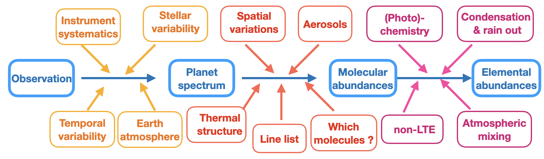
Figure 11: Flow chart showing the different steps needed to go from an exoplanet observation to an atmospheric elemental abundance measurement.

3.2.1 Brown Dwarf Abundances

Brown dwarfs (M$<$80M_J) provide a control sample for understanding the transition from “stellar” to “planetary” atmospheres. They are presumed to form like stars (see Whitworth et al., 2007, e.g.,), but unlike stars, they do not fuse H into He and they possess molecular dominated atmospheres (Figure 10, left) like planets. Under this assumption, it is expected that field brown dwarf elemental abundances should reflect the local stellar population. In effect, brown dwarfs are like non-irradiated planets, which greatly simplifies their observations (their spectra are not washed out by any host star) and the interpretation of their spectra. However, due to their molecular dominated atmospheres, extracting the atmospheric metallicities and abundance ratios is challenging.

Line et al. (2015, 2017) and Zalesky et al. (2019) leveraged the aforementioned atmospheric retrieval methods to apply a uniform retriaval/abundance analysis on homogeneous near-infrared spectra like those shown in Figure 10, left, to obtain constraints on the primary molecular constituents while taking into account the correlations/degeneracies between gas abundances, vertical thermal structure, gravity, radius, and instrumental artefacts. These works specifically focused on the cooler late-T-type brown dwarfs as they are observed (and predicted) to be largely cloud free (Burrows et al., 1997; Allard et al., 2001; Stephens et al., 2009) and the major carbon and oxygen bearing species are fairly homogenised in altitude, enabling a more pristine, less degenerate, abundance analysis. At these cooler temperatures ($<$800K) water, methane, ammonia, and potassium are the dominant trace gas constituents and hence, sculpt the dominant spectral features. From the abundance constraints on water and methane–the dominant oxygen and carbon-bearing species at these temperatures–the atmospheric metallicity ((CH₄+H₂O)/(M/H)_⊙) and carbon-to-oxygen ratios (CH₄/H₂O) can be derived. Figure 12 summarises these constraints on a sample of over 50 late T- and Y-dwarfs compared to the abundances from the local stellar population. Metallicity precisions between 0.2-0.5 dex and C/O constraints between 0.1 - 0.3 are readily achievable with low spectral resolution, high signal-to-noise, near-infrared spectra. The spread in abundances is comparable to the stellar population, but with an overall “offset” to higher C/O and lower [M/H] in the brown dwarf population. The condensation of silicates in the deep layers of the atmosphere provides a good explanation for this offset. Indeed, as shown by (Burrows and Sharp, 1999), the condensation of enstatite (MgSiO₃ and forsterite Mg₂SiO₄ should take between 2 and 3 oxygen atoms per magnesium atom out of the atmosphere. For solar abundance ratio of magnesium and oxygen, silicate condensation is therefore expected to decrease the number of oxygen atoms by 15 to 20$\%$ and thus increase the C/O ratio from, for example, 0.6 to 0.75. The condensation of other species, such as Fe₂O₃, if they indeed form, could increase the C/O ratio further to 0.85. Which condensates actually form in brown dwarfs and exoplanet atmospheres and in which quantities they form is, however, complicated to predict from first principles as both kinetics and microphysics processes can alter the predictions from chemical equilibrium.

The current focus is shifting towards the more data-rich, hotter, L-dwarfs (Burningham et al., 2017; Gonzales et al., 2020) of which present numerous additional absorbers, including CO, and metal hydrides/oxides enabling constraints on more elements. However, the hotter temperatures present numerous complicating factors including non-uniform vertical abundances and uncertain cloud opacities which can bias abundance determinations. Nevertheless, once these complications are understood, similar uniform abundance analyses/determinations as show in Figure 12 can be applied to a much larger sample ($\sim$1000) of objects providing an invaluable control sample for understanding the gradient between star and planet formation.

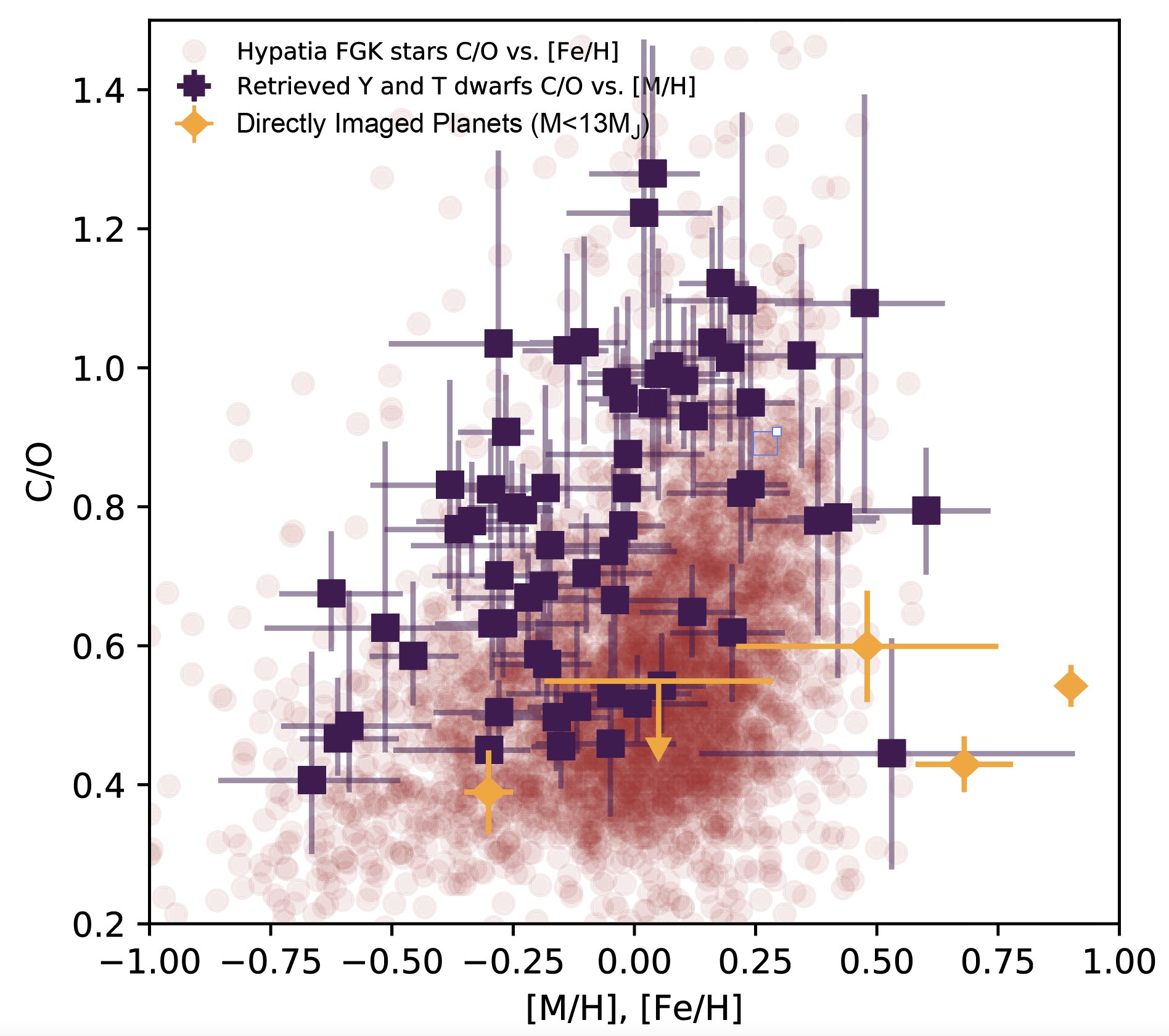
Figure 12: Brown Dwarf (dark blue) and directly imaged planet abundances (orange) compared to those derived for stars (red, Hinkel et al. (2014)). The brown dwarf abundances here are derived from a uniform atmospheric retrieval analysis (Line et al., 2017; Zalesky et al., 2019) applied to $\sim$50 late T and Y-dwarf low-resolution (R$\sim$120) spectra (Zalesky et al. in prep) to derive the atmospheric metallicity ([M/H]) and carbon-to-oxygen ratio. The directly imaged planet abundances are derived from a variety of sources given in the text. Such analyses on brown dwarfs provide a control sample for interpreting the abundances of exoplanets.

3.2.2 Directly-Imaged Giant Planet Abundances

“Directly imaged planets” generally refer to self-luminous, young, typically high mass planets ($\sim$few - 13M_J) that are observed at wide separations ($\sim$10-100 au) from their, typically young, host star. Coronographic techniques that suppress the scattered star light are needed in order to detect the oft less than 1 part in 10,000 thermal glow. Their masses straddle the classic evolutionary defined boundary between “planet” (e.g., low entropy, rocky cored) and “brown dwarf” (high entropy, degenerate) (Burrows et al., 1997). They provide unique tests of planet formation theories as both brown dwarf-like and solar system-like formation mechanisms (see §4) can explain their masses and orbital properties. Determining their atmospheric abundances and comparing them to those obtained from the brown dwarf population and the transiting exoplanet population (more below) can shed insight into their possible formation avenues. We refer the reader to Chapter XX (Currie et al.) for more details on the characterization of these worlds, we discuss them here in the context of their abundances.

Unfortunately, owing to the challenges in obtaining contrasts below 10^-6 and the very likely low occurrence rates of such types of planets ($\sim$10% for 5-13M_J at 10-100 au around $>$1.5M_⊙ stars, Nielsen et al. (2019)), only about ten have been spectroscopically characterised. Their spectra (Figure 10) are similar to those of brown-dwarfs suggesting that they possess similar opacities. While several key carbon and oxygen bearing molecules like CO, water, and methane have been been detected (see Table 1), determining their abundances has been challenging owing to their cloudy atmospheres and lower signal-to-noise spectra than their more readily observable brown dwarf cousins. Modelling assumptions tend to influence the reported abundances, usually derived from a combination of atmospheric retrieval modeling that provide direct constraints on the molecular abundances (Lavie et al., 2017; Wang et al., 2020) and 1D radiative-convective model grid fits (Konopacky et al., 2013; Barman et al., 2015), of which typically assume thermochemial equilibrium molecular abundances, and instead fit directly for the metallicity and C/O. Considering only the directly imaged planets with masses less than 13$M_{J}$, there are only 5 objects with reported metallicity and C/O constraints (Gravity Collaboration et al. (2020); Mollière et al. (2020); Wang et al. (2020); Petrus et al. (2021) and Chapter XX)). These constraints are shown in comparison to the stellar and brown-dwarf populations in Figure 12. With only five objects, it is difficult to readily discern any clear patterns/differences between the imaged planet population and the brown dwarfs–perhaps the imaged planet population is slightly metal enriched with somewhat lower carbon-to-oxygen ratios, though a much larger sample size is needed to make any confident statements.

However, it is worth being wary of the actual uncertainties on these abundance constraints due to the model assumptions used to derive them (e.g., see Wang et al. (2020)). Furthermore, the brown dwarf abundances were largely derived directly from the water and methane abundance constraints where-as most of the directly imaged planet constraints arise from the self-consistent grid fitting, with the latter typically resulting in artificially precise constraints owing to the radiative-convective-thermochemical equilibrium assumption within the models.

3.2.3 Transiting Planet Abundances

Transiting planets make up most of the charcterised exoplanet population, with thousands of Hubble orbits and thousands of Spitzer and ground-based telescope hours spent observing many dozens of atmospheres ranging from small cool terrestrial worlds to planets with hellish star-like atmospheres. It is this planet population that has driven most of the exoplanet-atmosphere literature.

Table 1: Chemical species detected in exoplanet atmospheres as of March 2022. We included only planets where more than 2 species have been detected and species that have been detected in at least two planets. We did not include species detected via photometry alone. Additional rock species (Ti,Sc,Si), ionised and non-ionised species and references are provided in the Appendix (see Table 4)

In contrast to brown dwarfs and directly imaged planets, due to their close-in orbits , the spectra of transiting planets cannot be measured directly, but rather, relative to their host stars. The wavelength-dependent opacity structure can be measured either when the planet passes behind its’ host star, an eclipse (an emission spectrum, or planet-flux/stellar-flux) or when the planet passes in front of its’ host star, a transit (transmission spectrum, the planet-to-star area or radius ratio) (Deming et al., 2019) (Figure 10, right two panels). Most transiting exoplanet atmosphere characterization stems from observations with the Hubble and Spitzer Space Telescopes. An alternative approach leverages the high orbital velocity of the planets, due to their short periods, which a time-dependent Doppler shift of the planetary molecular/atomic lines relative to the stellar and telluric lines enabling the use of large aperture ($>$ 6 m), high spectral resolving power (R$>$25,000), ground-based platforms (Birkby, 2018). This approach enables the characterisation of short-period non-transiting planets as well. As with the spectra of brown dwarfs and directly imaged planets, information about the abundances can be ascertained through various atmospheric retrieval (Madhusudhan, 2018) methods applied to the eclipse, transit, or high resolution Doppler spectra (Brogi and Line, 2019). Below we summarise the current state of species detections, and subsequent abundance determinations within the transiting planet population.

Table  1 summarises the various gaseous species detected in exoplanet atmospheres, with transiting planets, owing to their broad diversity in temperature and size, making up a bulk of the detections. Whether a given chemical species is detected in an atmosphere is determined by both by the intrinsic presence of that species as well as the instrumental set up (wavelength range, sensitivity). We separate the detected species into four categories: rocks, or elements that condense into solids for temperatures $<$1000K, alkalies, which have condensation temperatures between 500 and 800K, and finally, ices, which condense below 300K.

Water is ubuiquitous as it has been detected in most planetary spectra (Deming et al., 2013; Crouzet et al., 2014; Sing et al., 2016) observed with the Hubble Space Telescope. Due to the low resolution and relatively narrow wavelength coverage of the HST WFC3 instrument (1.1-1.4$\mu$m), no other molecular species beyond water have been reliably detected. Through the high-resolution ground based method, which can cover a broader range in wavelengths, carbon monoxide has been seen in only two transiting planets (Snellen et al., 2010; de Kok et al., 2013). Methane has yet to be reliably detected in all but a single planet, the hot Jupiter HD209458b (Giacobbe et al., 2021) and has yet to be found in cooler ($<$1000K) worlds (Stevenson et al., 2010; Kreidberg et al., 2018; Benneke et al., 2019) where it is expected to be more thermochemically prominent (Moses et al., 2013) (as is seen in similar temperature brown dwarfs, §3.2.1). Nitrogen bearing species have remained equally as elusive. That is because N₂, the main nitrogen bearing species in hot planets, does not have strong spectral lines. In cooler planets, NH₃ becomes the main bearer of nitrogen but has so far been detected only in a single hot planet, strongly out of chemical equilibrium(Giacobbe et al., 2021). HCN, thought to be a tracer of high carbon-to-oxygen ratios and/or photochemical processes has also been challenging to detect, but has been suggested to be present in at least one hot Jupiter (MacDonald and Madhusudhan, 2017; Hawker et al., 2018; Giacobbe et al., 2021)

Alkali metals have broad absorption lines in the optical that makes them observable at low spectral resolution from space (Sing et al., 2016) and at both low and high resolution from the ground (Huitson et al., 2017; Seidel et al., 2019; Nikolov et al., 2016). They are expected to condense out of the atmosphere around 800K and thus should not be observable in cooler planets.

More refractory material (“rocks”) can be observed in the hottest ($>$2000 K) of planets. In these ultra-hot Jupiters molecules thermochemically dissociate leaving behind numerous atomic species that can be observed at high spectral resolution (Lothringer et al., 2018; Parmentier et al., 2018; Kitzmann et al., 2018). Iron, magnesium, calcium and scandium have been observed in several planets (Vidal-Madjar et al., 2013; Yan et al., 2019; Ehrenreich et al., 2020; Borsa et al., 2021; Kesseli et al., 2022) whereas others such as yantium, nickel, titanium and chromium have only been seen in KELT-9b, the hottest known exoplanet (Hoeijmakers et al., 2019). Some of these species are also transported into the exosphere of the planet by the hydrodynamic escape of hydrogen and helium and get ionized. This leads to strong line-contrast for the observed ioninc species, such as Mg+ or Fe+, that can be observed in the near ultraviolet with HST (Sing et al., 2019).

Hydrogen and Helium have been seen in numerous planets, the former through the large Lyman-$\alpha$ and H$-\alpha$ absorption (Vidal-Madjar et al., 2003) and the second through the metastable Helium line around $1\mu m$ (Spake et al., 2018; Nortmann et al., 2018). These are usually seen very high in the atmosphere, up to the roche lobe limit of the planet, and are indicative of the presence of atmospheric escape (see Owen, 2019, for a review).

Measuring precise and accurate abundances, in contrast to pure detection, from current transiting planet spectra is not straightforward. Whereas the detection of a species is driven by the strength of the spectral lines, the measurement of the chemical abundances are driven by the shape of the spectral lines, which requires a higher signal-to-noise ratio. Again, retrievals are often used to leverage these spectral shapes to pull out quantifiable abundance constraints. However, at the level of precision needed to quantify abundances, several other nuisance phenomenon need to be accounted for within these retrieval methods. These include the presence of horizontal heterogeneities in temperature, chemistry and cloud coverage in the hottest targets, where the day-to-night thermal contrast can reach hundreds to thousands of degrees. Aerosols are always a cause of uncertainties in planetary spectroscopy, but this is particularly true for exoplanets where an enormous variety of condensates (Marley and Robinson, 2015; Helling et al., 2021) and photochemicaly produces hazes (Hörst et al., 2018; Kawashima and Ikoma, 2019) can potentially exist, combined with the long path lengths of starlight through the planetary limbs during transit (Fortney, 2005). The presence of aerosols can significantly change the scattering properties of the atmosphere and bias the abundance measurement (Deming et al., 2013; Taylor et al., 2021), particularly if they cover only part of the atmosphere (Line and Parmentier, 2016). For cooler planets (often discovered orbiting M dwarfs due to selection biases) the presence of stellar spots containing the very molecules one is trying to measure in the planet (e.g. water) leaves an imprint in the measured transit spectrum that can significantly bias the abundance measurements (Désert et al., 2011; Rackham et al., 2019).

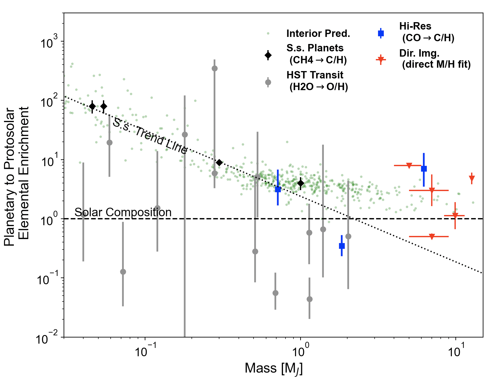
Figure 13: Atmospheric elemental abundance enrichment for select species as a function of planetary mass for the solar system planets (black diamonds), transiting exoplanets observed in transmission with the Hubble Space Telescope (grey circles, based on water/O constraints, Welbanks et al. (2019)), transiting (or near transiting) exoplanets observed with ground-based high resolution spectroscopy (blue squares based on CO/C constraints–(Brogi and Line, 2019; Pelletier et al., 2021, Line et al. 2021)), and directly imaged self-luminous planets (red triangles, based on direct grid fitting determined enrichments, Gravity Collaboration et al. (2020); Mollière et al. (2020); Wang et al. (2020); Petrus et al. (2021) and Chapter XX). The green scatter points are the interior structure based envelope enrichment predictions (Thorngren et al., 2016) for the observed exoplanet population assuming a 10/90% partitioning of metals in the envelope/core–similar to what is assumed for Jupiter. A linear fit to the solar system abundance is shown as the dashed line (see Kreidberg et al. (2014)). As of yet, there is no clear trend in envelope metal enrichment vs. metallicity among the characterised exoplanet population.

Despite water being readily detected, there is a large diversity in the signal strength resulting in a very wide range in the retrieved gas mixing ratios (see fig. 13). Several planets may have sub-solar oxygen abundances (Welbanks et al., 2019), as traced with water, and most planets seem to be less enriched in heavy element species than in the atmospheres of solar-system planets with similar masses, in contrast to what is derived for the population wide bulk planetary enrichments (Fig. 9). However, whether this inconsistency and the scatter in retrieved abundances is due to a scatter in intrinsic elemental abundances or a uncertainty in some of the other, poorly controlled parameters mentioned above, is not yet understood.

In the near future new instruments such as those on-board the James Webb Space Telescope or high-resolution instruments on the ground (such as IGRINS, ESPRESSO, CRIRES+, MAROON-X, SPIRou) should provide enough spectral information to break some of the common absolute-abundance inhibiting degeneracies. At the same time our theoretical understanding of these atmospheres should increase trust in our prior assumptions, leading to a better mitigation of nuisance parameters and thus more reliable abundance constraints.

3.2.4 Transiting Planets Abundance Ratios

Elemental abundance ratios are in theory more readily constrained than absolute abundances due to the lessened sensitivity of these ratios to common degeneracies (Benneke and Seager, 2012; Griffith, 2014). However, in practice, most instruments have too narrow a wavelength coverage to simultaneously measure the spectral features of multiple molecules and thus rely upon multiple visits with different instruments (Sing et al., 2016). However, as discussed above, the only major volatile species reliably detected with HST is water. Extracting information on the atmospheric metallicity and other elemental ratios like C/O or N/C, etc., is challenging if only “O” is being measured owing to the degeneracy between overall metallicity and the ratios themselves (e.g., a high metallicity and high C/O can produce the same O abundance as solar composition, Moses et al. (2013)).

Despite this challenge, there are several broad conclusions, primarily driven by the water/oxygen abundance itself and the lack of presence of expected carbon bearing species (namely, CH4) over the HST wavelength ranges, observed in transmission (where we have the most observations, upwards of two-dozen planets). Firstly, in most hot Jupiters (Tsiaras et al., 2018) water (hence oxygen) is abundant enough to present absorption stronger than the obscuring presence of H2-H2/He collision induced opacity, typically requiring values above 1 ppmv. Secondly, the shape of the water absorption feature relative to the collision-induced continuum for many planets is indicative water abundances that are below the stellar (usually solar) values, suggesting a “depletion” of oxygen (Madhusudhan et al., 2014a; Barstow et al., 2017; Pinhas et al., 2019; Welbanks et al., 2019) relative to solar and/or planet formation model atmospheric enrichment predictions (Fig. 13). Whether or not this apparent depletion of O is due to low overall metal enrichment or due to elevated C/O, remains to be seen. Furthermore, the degeneracy between the water abundance and cloud properties prevents constraints better than $\pm$1dex for most planets.

Nevertheless, inferences of carbon-to-oxygen ratios have been attempted by leveraging the lack-of-carbon species. Low C/O values have been presumed in two cool ($<$900K) worlds, GJ3470 (Benneke et al., 2019) and WASP-107b (Kreidberg et al., 2018), primarily owing to th elack of expected methane over the HST WFC3 pass-band. These works suggest sub-solar C/O ratios ($<$0.4), however, additional complications in these lack-of-methane based C/O inferences are strongly dependent upon the chemical assumptions (e.g., see Fortney et al. (2020))

Thermal emission/secondary eclipse (which probes the planetary dayside thermal emission) derived inferences are far less common due to the more difficult observational requirements (need hot enough planets to produce an observable spectrum). However, similarly, inferences derived from secondary eclipse observations with Spitzer and HST have provide comparable ambiguity. The broad-band (3 - 24 $\mu$m) Sptizer photometry observations the warm ($\sim$700K) Neptune, GJ436b (Stevenson et al., 2010), are suggestive of a methane depleted atmosphere (no methane at all detected), interpreted as either being due to disequilibrium (Stevenson et al., 2010) chemistry or extreme ($>$300$\times$Solar) metal enrichment (Moses et al., 2013). However, Spitzer photometry alone is not enough to thorughly break this degeneracy. Furthermore, this planet is too cool to be observed in eclipse with HST in the near-IR and the transmission spectrum of this world is relatively featureless (Knutson et al., 2014), providing little further insight into its composition.

The first evidence of a “high C/O” planet (C/O$>$1) arose from a combination of a featureless (blackbody) dayside WFC3 emission spectrum and Spitzer photometry of the ultra-hot ($\sim$3000 K) Jupiter, WASP-12b (Madhusudhan et al., 2011). However, this result is entirely dependent upon the reliability of the Spitzer eclipse depths, which are challenging to derive (Cowan et al., 2012) due to the oblate shape of the planet, nor did this initial interpretation consider key opacity sources expected to be present at such extreme temperatures (Parmentier et al., 2018), which could also explain the lack of water feature. Furthermore, the HST WFC3 transmission spectrum (Kreidberg et al., 2015) largely rules out the high C/O scenario, suggesting a composition consistent with solar.

Three planets, namely the hot Jupiters WASP-43b (Kreidberg et al., 2014), HD209458b (Line et al., 2016), and HD189733b (Zhang et al., 2020) present the most complete emission spectra and produce O enrichments that are consistent with solar. Retrievals on the the former two are consistent with a broad range of oxygen enrichements (0.6-8$\times$Solar, 0.06-10$\times$Solar, respectively), but provide little to no constraint on carbon-species leaving the degeneracy between metallicity and C/O un-broken. The latter spectrum, HD189733b, is suggestive (Zhang et al., 2020) of a metal enrichement of 8-20$\times$Solar and a $0.6<C/O<0.7$ under the assumption of thermochemical equilibrium chemistry (however, see Lee et al. (2012); Line et al. (2014) ). Placing unambiguous constraints on the elemental abundance ratios would require the detection of multiple elemental species.

Complimentary to the space-based HST and Spitzer based inferences, high-resolution ground-based observations (see review by Birkby (2018)) have provided an opportunity to detect both carbon and oxygen, and very recently, to provide constraints on their (3 transiting planets and one non-transiting, see Fig 13) abundances (Brogi and Line, 2019). Retrievals on the CRIRES K-band dayside emission data for the hot Jupiter’s HD 189733b and HD 209458b (Brogi and Line, 2019) produce precise constraints on the CO abundances and stringent upper limits on the water abundance, which together point towards C/O$\sim$1. However, these results are potentially at odds with the near-solar constraints obtained from the aforementioned space based HST/Spitzer measurements (Zhang et al., 2020; Line et al., 2016).

Similarly, recent analysis of the SPIRou (Pelletier et al., 2021) observations the non-transiting massive planet, $\tau$ Boo b, placed a stringent upper limit ($\lesssim 10^{-6}$) on water and a very precise ($\pm$0.27 dex) constraint on the CO abundance, resulting in an extremely precise ($\pm$0.01) C/O=1. Very recently, (Line et al., 2021), using the IGRINS instrument, observed a generic transiting hot Jupiter ($\sim$1700K) WASP-77Ab obtained precise, bounded constraints on both the water and CO abundances, leading to a metallicity of 0.33$\pm$0.11 and a C/O=0.59$\pm$0.08. We anticipate comparable constraints over the next several years as more and more high resolution observations are obtained and analysis procedures developed.

Isotpologue ratios can be measured in exoplanetary atmospheres by resolving the spectral lines of different isotopologues. This has been performed on carbon monoxide, with the $\rm{}^{13}CO/^{12}CO$ ratio measured to be about 3 times higher than the solar-system value in both the young massive planet TYC 8998-760-1 b using VLT/SINFONI  (Zhang et al., 2021b) and the hot Jupiter WASP-77Ab (Line et al., 2021). It has also been measured with Keck/NIRSPEC in a young brown dwarf, 2MASS J03552337+1133437, where it is consistent with the solar value (Zhang et al., 2021a). While there has yet to be a unifying interpretation of these results alone (see § 4.3.3), isotopic fractionation will provide an addition dimension to constrain planet formation history.

Certainly, we cannot discuss all compositional inferences within this chapter, we highlight works that elucidate some of the key issues in the field. Fig. 13 is an attempt at summarising the state of the abundances in terms of metal enrichment’s of the various planet populations (transiting, directly imaged) and techniques (low res space based, hi-res ground based,direct imaging). We also urge caution when interpreting the ensemble of results as different analysis on different datasets can often result in conflicting conclusions. As we obtain higher quality data, expected on all fronts, we anticipate a convergence in our overall understanding of atmospheric abundances.

3.3 Linking bulk and atmospheric abundances

Whether the observed atmospheric abundances are representative of convective envelope abundances depends on how deep is the radiative/convective boundary situated and how strong is the vertical mixing in the radiative zone. The timescale for mixing elements accross the radiative zone can be estimated as:

$$\tau_{\rm mix}=\frac{(nH)^{2}}{K_{zz}},$$ (3)

where $nH$ is the distance between the photosphere and the radiative/convective boundary expressed in units of the scale height and $K_{zz}$ is the vertical mixing coefficients.

For Brown Dwarfs and directly imaged planets the photosphere is situated very close to the radiative/convective boundary and no elemental diffferences are expected between what we observe and the convective zone. For close-in planets, however, the strong stellar irradiation leads to the formation of a radiative zone that can extend down to 1000 bars for planets with a Jupiter-like internal flux (§ 3.1.1), which situates the radiative/convective boundary roughly 10 scale heights away from the photosphere. Hot inflated planets likely have a much larger internal flux than Jupiter which would raise the radiative/convective boundary much closer to the photosphere (Thorngren and Fortney, 2019).

The vertical mixing in the radiative zone of close-in planets is driven by the strong day-to-night atmospheric circulation induced by the inhomogeneous day/night heating(Parmentier et al., 2013; Sainsbury-Martinez et al., 2019), the presence of shear instabilities(Li and Goodman, 2010; Fromang et al., 2016; Menou, 2019), shocks (Heng, 2012) or gravity waves (Watkins and Cho, 2010). The strength of most of these mixing processes increase with decreasing pressure (Menou, 2019), meaning that the bottleneck for vertical mixing is likely situated at the radiative/convective boundary itself. An estimate for the mixing timescale accross the radiative zone can therefore be obtained by estimating the time to cross one scale height at the radiative/convective boundary. Whereas estimates from shear instabilities alone lead to values of $K_{zz}$ close to $10$m²/s (Menou, 2019) at 100 bars, estimates based on the overturning circulation are much larger, reaching $10^{5}$m²/s (Parmentier et al., 2013) and possibly higher (Heng, 2012; Sainsbury-Martinez et al., 2019). Using equation 3 with a scale height of 500km we obtain that mixing timescale to cross one scale heights should less than $\approx 30$ days for a mixing driven by the overturning circulation but up to $100$ years for a mixing driven by shear instability only, both significantly shorter than the planet evolution timescale. This comparison indicates that the radiative zone should not be a great barrier to transport and thus that the atmospheric abundances should be a good proxy for the abundances in the convective zone. However these estimates are very uncertain because we do not understand yet the deep atmospheric circulation in hot Jupiter atmospheres.

Some chemical species expected to be in gaseous phases in the dayside atmosphere can condense on the nightside or in the deep atmospheric layers (Spiegel et al., 2009; Parmentier et al., 2013). Gravitational settling is then in competition with the vertical mixing to determine whether these species are trapped below the photosphere. The efficiency of the gravitational settling depends on the particle size distribution and particularly to the largest possible size of cloud particles. Current models indicate that coagulation play a much smaller role in hot giant exoplanet clouds, due to the low mixing ratio of the cloud condensing materials (e.g. Fe, Mg, Si) compared to the mixing ratio of water in Jupiter for example. As a consequence, clouds in hot exoplanet atmospheres are not believed to grow particles larger than $\approx 100\mu m$ (Lee et al., 2016; Woitke et al., 2020; Powell et al., 2019), which can lead to a significant reduction of the dayside atmospheric abundances compared to local chemical equilibrium (Spiegel et al., 2009; Parmentier et al., 2013; Beatty et al., 2017) but not completely deplete the atmosphere of this species (Powell et al., 2018). Such a mechanism has been proposed to explain the apparent lack of TiO in several planets (Beatty et al., 2017).

By comparing the atmospheric metallicity measured from the spectra of the planet to the bulk metallicity inferred from its mass, radius and age, one can estimate how heterogeneous is the planet interior (Thorngren et al., 2016; Thorngren and Fortney, 2019). As we show in Figure 13 coreless models with fully mixed interior lead to predicted atmospheric metallicities that are much larger than the measured one, both in solar system and in exoplanets. Overall, between $50\%$ and $99\%$ of heavy elements must be sequestered below the photosphere, either in the envelope or in the core of the planet, in order to reconcile atmospheric and bulk measurements.

4 CONSTRAINING GIANT PLANET FORMATION

Since giant planets are dominated by hydrogen and helium, they must form when the circumstellar gas disk is still present, within a few million years of the formation of the central star. We first present a few theoretical aspects of the formation of giant planets, then examine what we can learn from solar system and giant exoplanets, and provide perspectives for future progress.

The formation mechanism of giant planets is still being investigated. There are two main formation models known as ”core accretion” and ”disk instability” (see Wuchterl et al., 2000; Durisen et al., 2007; Lissauer and Stevenson, 2007; D’Angelo et al., 2010; Helled et al., 2014b; Nayakshin, 2017; D’Angelo and Lissauer, 2018; Mordasini, 2018; Helled and Morbidelli, 2021, for reviews, and references therein). In the core accretion model the formation of giant planets begins with the buildup of a heavy-element core. The core is formed via the accretion of solids that can be in the form of planetesimals and/or pebbles. The composition of these solids depends on the formation location of the growing planet due to the existence of various ice lines. In the disk instability model, giant planets form via local gravitational instability in the disk which leads to fragmentation. The forming objects must cool down and contract fast enough to remain gravitationally bound. The expected masses and orbital properties of the objects formed via this mechanism are still being debated. Often this formation path is required to explain giant planets around M-stars, massive giant planets at very large radial distances, and massive planets around very young star (Durisen et al., 2007; Helled et al., 2014b). Nevertheless, core accretion is the standard formation model and the expected mechanism for the formation of the giant planets in the solar system.

4.1 The Stages of Planetary Growth

The different stages of the formation and growth of a giant planet such as Jupiter as originating from the work of Bodenheimer and Pollack (1986) and Pollack et al. (1996) are presented in Fig. 14. After a first disk phase, a core forms and grows. As the core’s gravity becomes strong, a hydrogen-helium dominated envelope progressively contracts and grows. When a cross-over mass of $\sim 20-30\rm\,M_{\oplus}$ is reached, the envelope’s self-gravity dominates over the core’s gravity, triggering a runaway gas accretion limited by the cooling and contraction of the envelope. When the envelope mass reaches $\sim 100\,\mathrm{M}_{\oplus}$, the envelope growth becomes limited only by disk supply (Tanigawa and Watanabe, 2002; Tanigawa and Ikoma, 2007). When gas accretion stops, the giant planets enter a late evolution phase with limited growth (although impacts, and particularly giant impacts may occur), but in which their interior still evolves. The timescales of these different phases are not well-defined and should highly depend on the systems considered. In the solar system, meteoritic constraints indicate that the inner solar system has been separated from the outer system between about 1 Myr to 4 Myr after the formation of the first condensates, which is interpreted as marking the times of Jupiter’s core formation and rapid envelope accretion phases, respectively (Kruijer et al., 2020).

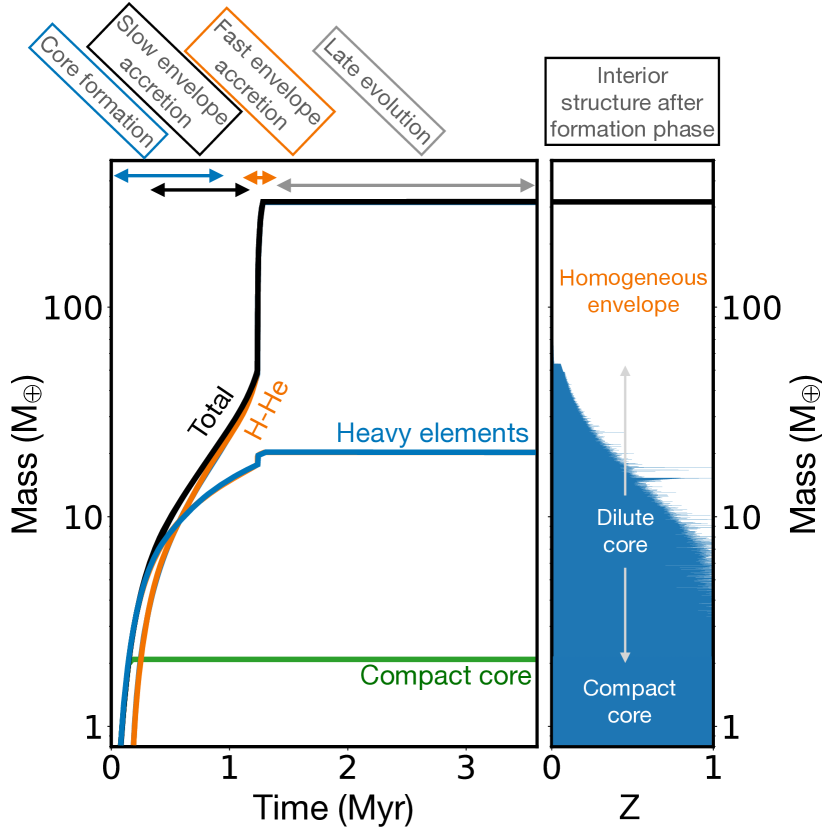
Figure 14: The stages of planetary growth based on the calculations presented by Lozovsky et al. (2017). The left panel indicates the evolution with time of the masses of the compact core, heavy elements and hydrogen and helium in a forming Jupiter-mass planet. The timescales are only illustrative. The right panel shows the interior structure in heavy element mass fraction $Z$ (in blue) as a function of interior planetary mass at the end of the formation phase. Four phases are identified. The core formation phase leads to the formation of first a compact core and then of a dilute core when planetesimals and pebbles dissolve in the envelope. It overlaps with the slow envelope accretion phase. The fast envelope accretion phase may be extended if the gas supply becomes limited (see text).

These stages of planetary growth are presented in more details hereafter.

4.1.1 The Protoplanetary Disk

Planets form by collecting material from a circumstellar/protoplanetary disk. A simple picture for the radial composition of such a disk is shown in Fig. 15, highlighting the carbon-to-oxygen (C/O) and refractory-to-volatile (R/V) ratios in gas and solids as functions of distance to the central star. Here it is assumed that the protoplanetary disk inherits the molecular abundances from the molecular cloud core from which the star and protoplanetary disk originated; the composition of gas and solids is determined almost solely by condensation of the molecules H₂O, CO₂, CH₄ and CO (e.g., Öberg et al., 2011; Eistrup et al., 2016). Simple to understand is the dependence of the R/V ratios in gas and solids on the radial distance to the central star: The R/V ratio in gas (solids) increases (decreases) with the radial distance because more volatiles condense and are, thus, removed from gas (added to solids) in the outer regions.

However, one has to consider several complications. First, materials are to some extent chemically processed during the gas accretion from molecular clouds onto protoplanetary disks. The subsequent chemical reactions in the protoplanetary disk lead to different chemical abundances in gas and solids (Eistrup et al., 2016; Cridland et al., 2019a, b). Temperature may not monotonically decrease with radial distance to the central star, and there may be local cold regions in protoplanetary disks (Ohno and Ueda, 2021). In addition, planet formation takes place in an evolving protoplanetary disk (e.g., Hueso and Guillot, 2005; Ida and Lin, 2004). Decline in gas surface density and viscous accretion heating results in a displacement of the ice lines (Min et al., 2011; Oka et al., 2011). While kilometer-size and larger planetesimals are expected to remain in place (Weidenschilling, 1977), dust and pebbles drift radially, sublimate and recondense near ice lines (e.g., Ciesla and Cuzzi, 2006; Hyodo et al., 2021), causing a redistribution of material and a change in the C/O and R/V ratios (Booth et al., 2017; Booth and Ilee, 2019; Schneider and Bitsch, 2021a, b). Because giant planets remain efficient gas accretors even after gap opening (Tanigawa and Ikoma, 2007; Tanigawa and Tanaka, 2016; Dürmann and Kley, 2017), the fate of the disk gas is also an important, often forgotten, part of the story. The fact that disk photoevaporation takes place in regions devoid of grains leads to a progressive change in the overall metallicity and possibly composition of the gas disk (Guillot and Hueso, 2006; Monga and Desch, 2015; Atreya et al., 2018). These complications must be considered to predict and analyze the final elemental abundances in giant planets and their atmospheres.

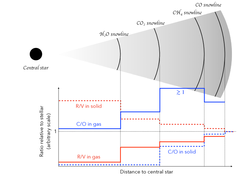
Figure 15: Schematic profiles of elemental abundance in a quiescent initial protoplanetary disk, which are determined solely by the “snow” lines for H₂O, CO₂, CH₄, and CO (made following e.g., Eistrup et al. (2016)). The blue solid and dashed lines represent the carbon-to-oxygen (C/O) ratios in gas and solids, respectively. The red solid and dashed lines represent the refractory-to-volatile (R/V) ratios in gas and solids, respectively.

4.1.2 Core formation

Traditional core accretion models assumed that giant planet cores have masses of tens of Earth masses in order to initiate rapid gas accretion (i.e., critical-mass cores) (e.g., Mizuno, 1980; Pollack et al., 1996). Recent models, however, estimate that cores first formed are rather small. The smaller the opacity in the envelope, the smaller the critical core mass is (Ikoma et al., 2000; Hubickyj et al., 2005; Valletta and Helled, 2021). Rapid gas accretion with smaller core masses can be a result of various physical processes such as faster cooling of the protoplanet due to settling of dust grains leading to lower opacity (Podolak, 2003; Movshovitz et al., 2010; Ormel, 2014) and the enrichment of the envelope with heavy elements which increases the mean molecular weight of the envelope leading to faster contraction (e.g., Hori and Ikoma, 2011; Venturini et al., 2016).

Second, the critical core mass is strongly dependent on the composition of the envelope and can be of the order of a few Earth masses. Heavy element enrichment (or contamination) of the envelope leads to reducing the critical core mass and the timescale of runaway gas accretion, because the mean molecular weight becomes large, the specific heat is reduced, and endothermic reactions including condensation occur (e.g., Hori and Ikoma, 2011; Venturini et al., 2015, 2016; Brouwers et al., 2018; Kimura and Ikoma, 2020; Valletta and Helled, 2021). The envelope enrichment likely occurs because planetesimals and/or pebbles are captured by the envelope itself (e.g., Inaba and Ikoma, 2003; Okamura and Kobayashi, 2021; Valletta and Helled, 2021) and subject to ablation and vaporisation on the way toward the core (e.g., Podolak et al., 1988; Valletta and Helled, 2020; Brouwers and Ormel, 2020). Recent simulations of collisional growth from dust grains to gas giant cores show that solids of different sizes contribute to core formation (Kobayashi and Tanaka, 2021). Thus, the contamination of the protoplanetary envelope by incoming solids and its feedback on planetary growth now appears to be an essential part of the formation of giant planets. Those recent studies put together, the structure of a proto-giant planet in early stages of accretion may be such that there is a relatively small central core (of a few M_⊕) surrounded by an envelope highly contaminated with heavy elements (Lozovsky et al., 2017; Helled and Stevenson, 2017; Valletta and Helled, 2019).

4.1.3 Gas accretion

As the protoplanet grows in mass, it can accrete gas from the surrounding disk. The composition of the gas is expected to be dominated by H-He, and is often assumed to have a proto-solar composition. However, depending on the planetary formation location, other volatile elements can also be in the gaseous phase, and therefore phase and therefore lead to an enrichment of the atmosphere. During the early stages, when the proto-planet mass is low ($\sim\leq 30$ M_⊕) the gas accretion rate is moderate and is determined by the cooling rate of the protoplanet (see e.g., Bodenheimer and Pollack, 1986; Ikoma et al., 2000; Helled et al., 2014b, for details). When the planet becomes massive enough, gas accretion rate is greater than the amount of gas that the disk can supply (e.g., Tanigawa and Watanabe, 2002) (also known as the ”detached phase”).

In this later stage of runaway accretion, the gas accretion rate is given by prescriptions based on hydro-dynamical simulations (e.g., Lissauer et al., 2009). The mechanisms that terminate gas accretion and determine the final planetary mass are still being investigated (e.g., Tanigawa and Ikoma, 2007; Tanigawa and Tanaka, 2016), with the most common explanations being gap formation and disk dissipation.

4.1.4 Late heavy-element accretion

Most of the heavy-element enrichment of giant planets in the core accretion model occurs during the buildup of the core. However, further enrichment can take place at later stages. When planetesimals are embedded in a protoplanetary gaseous disc, the combination of gravitational enhancement and gas drag damping of their random velocities results in widening the separation between the planetesimal and protoplanet (e.g., Tanaka and Ida, 1997). An increase in the protoplanet mass via runaway gas accretion leads to widening the protoplanet’s feeding zone which helps the protoplanet to capture more planetesimals; however, its efficiency is not high enough to collect tens of Earth masses of solids (Zhou and Lin, 2007; Shiraishi and Ida, 2008; Shibata and Ikoma, 2019), unless extremely large amounts of solids are available.

However, as originally proposed by Alibert et al. (2005), a much wider feeding zone and thus many more planetesimals are accessible if the proto-giant planet is migrating. A complication arises however, the trapping of planetesimals in sweeping mean motion resonances with the migrating gas-giant planet (e.g., Tanaka and Ida, 1999). With dedicated dynamical simulations Shibata et al. (2020) demonstrate that the capture of planetesimals takes place only in limited regions of the disc because of the effects of resonant and aerodynamic shepherding. This so-called sweet spot depends on many parameters including planetesimal size and disc properties, but should be located in the 3-10 au region, possibly extending to 30 au for nominal values of the parameters (Shibata et al., 2022). Thus, planets having crossed that region - in particular those having migrated from large distances would tend to have captured more planetesimals, possibly tens of Earth masses.

Another mechanism, the accretion of pebbles is strongly suppressed in the giant planet regime because the planetary gravitational perturbation results in regions with super-Kepler rotation speeds exterior to the orbit of the planet (Lambrechts et al., 2014). Instead, if drifting pebbles drift in and vaporise inside the snowline, the growing gas giant would accrete disc gas that is contaminated with heavy elements, thus possibly ending-up metal rich (Booth et al., 2017). For this mechanism to work, the planet must be inside the snowline and the metal-poor gas in the outer disk must be lost, possibly by photoevaporation (see Guillot and Hueso, 2006, and § 4.3.2). .

Finally giant planets may also accrete heavy elements after all the gas has dissipated. Calculations for the solar system giant planets indicate that only limited amounts ($0.2\,M_{\oplus}$ or less) would be accreted (Matter et al., 2009). However, it is interesting to notice that for a planetesimal in the outer solar system, its ejection probability is much higher than its accretion probability, mostly because the escape speed at Jupiter is much larger than its orbital speed (by a factor $\sqrt{2(M_{\rm p}/M_{\star})(R_{\rm p}/a_{\rm p})}\sim 4.6$ where $M_{\rm p}$ and $R_{\rm p}$ are the planetary mass and radius, $M_{\star}$ the stellar mass and $a_{\rm p}$ the planet orbital distance). The ejection probability becomes negligibly small when the planet escape speed becomes smaller than the orbital speed, i.e. when $M_{\rm p}\leq(1/2)(R_{\rm p}/a_{\rm p})M_{\star}$. For a solar-type star and a Jupiter-radius planet, this corresponds to $M_{\rm p}\sim 17\,M_{\oplus}$ at 5 au and to $M_{\rm p}\sim 2.7\,M_{\rm Jup}$ at 0.1 au (Guillot and Gladman, 2000). When not accompanied by other giant planets, hot Jupiters should be efficient accretors of planetesimals and planets.

4.2 Evolution of a formed planet

4.2.1 Importance of primordial entropy and thermal state

Traditional giant planet formation models often over-simplify the treatment of the accretion shock associated with runaway gas accretion. During this late stage most of the planetary mass is accreted and the influence of the accertion shock on the planetary thermal state and consequent evolution is of high importance (e.g., Marley et al., 2007; Marleau et al., 2017; Mordasini et al., 2017; Berardo et al., 2017; Berardo and Cumming, 2017; Cumming et al., 2018).

Depending on the assumptions made regarding the accretion shock, it was shown that the accreted H-He gas can have much higher entropy than the interior of the accreting protoplanet (Berardo and Cumming, 2017; Cumming et al., 2018). This results in a large radiative region. This region can become convective after several Myrs as the planet contracts and cools down. The fact that the deep interior is expected to have composition gradients that also act towards inhibiting convection suggest that giant planets starts their contraction having large non-convective regions. As a result, the onset of convective mixing is expected to be delayed. It is therefore clearly desirable to include the primordial entropy profiles when studying the evolution and current-state of giant planets.

Progress can also be achieved through direct observations of young objects. Probably the best example is the young ($\sim 21$ Myr-old) giant planet $\beta$ Pic b, which was detected by direct imaging (Lagrange et al., 2010; Bonnefoy et al., 2013) and whose mass, $11\pm 2\rm\,M_{Jup}$, was measured via astrometry (Snellen and Brown, 2018). The large brightness of $\beta$ Pic b indicates that it was formed ”hot”, i.e. with a limited loss of entropy during accretion (e.g., Bonnefoy et al., 2013). Separately, H$\alpha$ emission has been detected for the young gas giants PDS 70 b and c ($<$ 10 Myr old; Wagner et al., 2018; Haffert et al., 2019; Hashimoto et al., 2020), indicating the presence of an accretion shock. Models of the late-stage accretion of gas by forming planets show that explaining the observations requires an accretion flow occurring on a small fraction of the planetary surface and with a significant entropy loss (Aoyama et al., 2018; Aoyama and Ikoma, 2019; Marleau et al., 2019; Takasao et al., 2021; Aoyama et al., 2021). The masses of PDS 70 b and c being unknown, it is however too early to understand whether this result is in tension with the $\beta$ Pic b result or whether it may apply to a different class of planets.

4.2.2 Re-distribution of Heavy-Elements during the Long-Term Evolution

In order to link the measured composition and current-state structure to the formation process, the long-term (timescales of $10^{9}$ years) evolution should be investigated. There are several processes that can change the distribution of chemical elements in giant planets such as convective mixing, settling and phase transitions.

If young giant planets consist of composition gradients, convective mixing can erode the gradient, and mix some of the heavy-elements to the outer convective regions. This in return, leads to an enrichment of the atmosphere with heavy elements. The mixing rate depends on the exact local conditions such as the shape of the gradient, the thermal state of the planet, and the mixing parameters. The initial entropy and primordial temperature profile determine the planetary evolution and the efficiency of convective mixing.

The evolution of Jupiter with composition gradients has been presented by Vazan et al. (2018)). In this model an evolutionary path that can lead to the current-state measured properties of Jupiter was consider. As a result, the primordial thermal state and internal structure have been inferred to fit Jupiter today and are not guided by formation models. It was shown that the outer part of the planet, $\sim$ 50% of Jupiter’s radius, becomes homogeneous after several $10^{6}$ years due to convective mixing. The erosion of the composition gradient enriches the planetary envelope with heavy elements, while Jupiter’s deep interior is found to remain stable against convection. It was then concluded that composition gradients which are stable against convection can persist for timescales of Gyr. This in return directly affect the planetary thermal structure and cooling history: in such a configuration the internal temperatures can be significantly higher than in the case of an adiabatic structure and the cooling of the planet is less efficient.

The primordial thermal state of the young Jupiter considered by Vazan et al. (2018) corresponds to a rather cold start which seems to be unrealistic according to planet formation models that simulate the the planetary growth and the accretion shock during the rapid gas accretion state. As a result, a thermal evolution model in which Jupiter’s growth from the onset of runaway gas accretion is considered was presented by Müller et al. (2020). Then the long-term evolution was simulated considering the energy transport and heavy-element mixing. Various formation conditions were investigated including different primordial composition gradients, heavy-element accretion rates, and shock properties. It was found that in all the models after several Myr most of Jupiter’s the envelope ($\sim$ 80% by mass) becomes convective and homogeneous. Fig. 10 shows the primordial and current-state heavy-element distribution of Jupiter as calculated by Vazan et al. (2018) and two of the formation models presented by Müller et al. (2020) which are hotter by $\sim 50\%$ throughout most of the envelope. Thus, according to the latter, composition gradients tend to be relatively compact, even when a substantial amount of heavy elements is accreted at late stages, unless a further mechanism, such as a giant impact takes place (Liu et al., 2019).

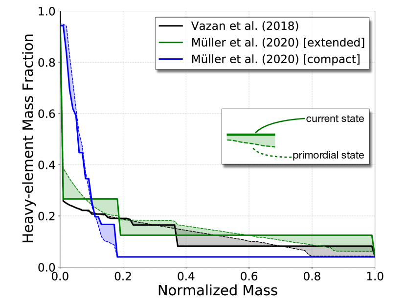
Figure 16: Heavy-element mass fraction vs. normalised mass of Jupiter shortly after its formation (dashed) and today (plain). The different curves show different models of Jupiter: the black lines correspond to the model of Vazan et al. (2018) while the green and blue lines to the hot-extended and hot-compact models of Müller et al. (2020). It is shown that 4.5 Gyr of evolution can significantly change the heavy-element distribution of giant planets, with the efficiency of mixing depending on the initial distribution of heavy elements and the thermal state of the young planet (see text for details).

4.2.3 Effect of phase transitions

Phase transtions can affect the structure and evolution of giant planets. This is in particular relevant for warm/cold giant planets that have internal temperatures that are low enough to experience such transitions as indicated in Fig. 2. The phase separation of helium in metallic hydrogen leads to an inhomogenous distribution of helium and an enrichment of helium in the deep interior and possibly the formation of a pure-He shell (e.g., Mankovich and Fortney, 2020). In addition, this process affects the energy transport by the creation of regions where heat is transported via conduction/radiation/semi-convection leading to non-adiabatic temperature profile that prolongs the planetary contraction. Other phase transtions linked to elemental solidification and solubility of mixtures can also play a role in giant planet evolution. Indeed, the low observed luminosities of Saturn are often explained by helium rain and composition gradients, respectively. Compositions gradients and boundary layers could also exist in Jupiter, Uranus, and Neptune. It should be noted that the combination of chemical phase transitions and composition gradients makes the modeling of giant planet interiors even more challenging (e.g., Vazan et al., 2016). We suggest that future structure and evolution models should consider phase transtions and their effect on the evolution and internal structure of giant planets.

4.3 Confronting Theory & Observations

4.3.1 Accounting for Atmospheric Abundances

While giant planet formation models have often focused on accounting for parameters such as core mass and bulk composition, some models also accounted for the measured atmospheric abundance. It was shown by Alibert et al. (2005) that if Jupiter migrated to its current location from $\sim$ 8 au, it could have accreted sufficient amount of planetesimals to explain Jupiter’s measured atmospheric composition, and predicting the O/H ratio in Jupiter to be six time solar. The authors have also followed the formation of Saturn and predicted the accretion of $\sim$ 13 M_⊕ of heavy elements in Saturn with at least 5.4 M_⊕ of ices.

Recent Jupiter formation models that assume core formation via pebble accretion followed by planetesimal accretion can also reproduce Jupiter’s atmospheric metallicity of $\sim$ 3 times solar (Alibert et al., 2018). Venturini and Helled (2020) have preformed a large parameter space study to explore under what conditions are needed for Jupiter’s heavy-element mass to be between 20 M_⊕ and 40 M_⊕, and found that Jupiter could have accreted 1–15 M_⊕ of heavy elements during runaway gas accretion, depending on the assumed initial surface density of planetesimals and the heavy-element accretion rate during the final stage of its formation.

The atmospheres of Uranus and Neptune are expected to be highly enriched with heavy elements. However, given the large uncertainties linked to their formation histories and bulk compositions (e.g., Helled et al., 2020b; Helled and Fortney, 2020, and references therein), we are still not a stage that atmospheric composition can constrain the planetary origin or vice versa. Future measurements of the atmospheric compositions and gravitational fields of the ice giants can be used to further constrain their structure, and formation path.

Jupiter’s enrichment in noble gases and in nitrogen (see Fig. 7), a major surprise from the Galileo probe, has been seen as a sign of the planet’s formation at very low temperatures $\sim 30\,$K (Owen et al., 1999). Instead, Guillot and Hueso (2006) proposed that it is a consequence of (i) the fact that noble gases stick to grains in the cold outer protoplanetary disk, (ii) that these grains migrate to the mid-plane and to the inner disk where the nobles gases which can be accreted as gas by the growing giant planets and (iii) that photoevaporation in the disk occurs at locations where grains have low abundances and therefore leads to a preferential loss of hydrogen and helium (and potentially neon, depending on the outer disk temperature). The model required a relatively late formation of the planet, in sync with the photoevaporation of the disk, but it has been proposed that grain migration can lead to increase metallicities locally, lifting somewhat this timing requirement (Monga and Desch, 2015; Mousis et al., 2019).

Finally, it should be noted that the observed enrichment could also be a result of post-formation accretion of heavy elements and/or the re-distribution of heavy elements from the deep interior. Therefore in order to link the atmospheric composition with the formation process it is critical to properly model the planetary evolution.

4.3.2 C/O and Other Abundance Ratios

In principle, the measurement of abundance ratios are a powerful way to understand how giant planets were assembled. Madhusudhan et al. (2014b) proposed to retrace the formation mode and migration history of giant exoplanets from their C/O ratio: They proposed that hot Jupiters with high C/O ratios and low O/H abundances should have been formed by disk-free migration. Ali-Dib et al. (2014) proposed that giant planets with envelopes accreted inside the water snowline should be carbon-rich (with a C/O ratio higher than that of the star). Mousis et al. (2014) proposed that Saturn’s low $\rm{}^{14}N/^{15}N$ value is indicative of a formation of its building blocks at 45 K in the solar nebula, predicting an O/H value of $\sim 34.9$ times protosolar and a $\sim 43.1\rm\,M_{\oplus}$ mass of heavy elements in the planet. Both Öberg and Wordsworth (2019) and Bosman et al. (2019) interpreted Jupiter’s near protosolar C/N ratio as an indication that Jupiter’s core assembled exterior to the N₂ snowline, echoing a similar conclusion made twenty years earlier (Owen et al., 1999, 2001). Cridland et al. (2020) concurred with this result, with an independent conclusion that, owing to its C/O and N/O ratios, Jupiter likely did not form in the inner 5 au in the solar system. Finally, Notsu et al. (2020) found that hot Jupiters with $\rm C/O>1$ can only form between the CO₂ and CH₄ snowlines, corresponding to locations between 2.6 and 16 au in a classical minimum-solar nebula.

These conclusions might be correct. Unfortunately, they result from models based on many underlying hypotheses, most of those untested. Using a planet population synthesis model based on planetesimal accretion, Mordasini et al. (2016) obtained planets with relatively low C/O ratios (0.1 to 0.5), but wisely noted that ”To link a formation history to a specific C/O, a better understanding of the disk chemistry is thus needed”. Booth et al. (2017) and Madhusudhan (2019) showed that outcomes of the C/O ratios and globally enrichments in giant exoplanets critically depend on whether giant planet growth occurs via accreting planetesimals or pebbles. Cridland et al. (2019b) showed that carbon-chemistry, a still unanswered puzzle in the solar system (e.g. Gail and Trieloff, 2017), can strongly modify the resulting planetary C/O ratios depending on the assumption used. Schneider and Bitsch (2021b) found that Jupiter’s nitrogen content can be explained by inward-diffusing nitrogen-rich vapour, so that Jupiter does not need to form close to the N₂ snowline, contrary to what inferred by Öberg and Wordsworth (2019) and Bosman et al. (2019). Separately we can also see that the new constraint on Saturn’s heavy element content (see Mankovich and Fuller, 2021, and § 2.4.1) rules out the clathrate model proposed by Mousis et al. (2014).

Clearly, we must acknowledge that giant planets result from a combination of many complex and uncertain processes. As we have seen (§ 4), we do not know the relative proportion of dust, pebbles and planetesimals that led to the present-day giant planets. Even assuming a fixed composition for the protoplanetary disk, we do not know the composition of planetesimals that are formed (e.g., Ida and Guillot, 2016; Hyodo et al., 2021). The growth of dust to pebbles leads to large-scale radial motions (a ”pebble wave”) and an evolving composition of disks (e.g. Booth and Ilee, 2019; Kunitomo and Guillot, 2021), probably in a complex time-dependent way (e.g., Elbakyan et al., 2020). Most importantly, giant planets are efficient gas accretors. This has two strong implications: heavy elements may be accreted as gas, inside of their snowline, and the photoevaporation of gas in the disk has an essential role in setting the final planetary masses (Tanigawa and Ikoma, 2007; Tanigawa and Tanaka, 2016) but also the final balance between heavy elements and hydrogen and helium in the planetary envelope (Guillot and Hueso, 2006; Monga and Desch, 2015; Atreya et al., 2018). Finally, as we have demonstrated in § 2.1, giant planets may not be fully convective. This implies that the composition of their atmosphere will be modified mostly by the late accretion phases rather than by the formation of their core as often implicitly assumed.

4.3.3 Isotopic Ratios

For our solar system giant planets, two isotopic ratios are most easily explained by invoking a partial mixing of the envelope and interior. The first one is D/H, a particularly important tracer of planetary formation because of its low value in the main reservoir H₂, and its high value (160 to 530 ppm) in cometary ices (Hersant et al., 2004; Bockelée-Morvan et al., 2015). The protosolar D/H is extremely difficult to determine due to its destruction in the Sun. Indirect inference from $\rm{}^{3}He/^{4}He$ measurements in the solar wind point to a low value $16.7\pm 2.5$ ppm (Table 3), but measurements in the local interstellar medium point to a value $>21$ ppm (Asplund et al., 2021, and references therein). The most accurate values obtained for Jupiter and Saturn are $22.5\pm 3.5$ ppm and $21\pm 1.3$ ppm, respectively (see Table 3). Assuming full mixing and a $\sim 300$ ppm D/H ratio in solids, we should expect an enrichment over the the protosolar value of $1$ to $4$ ppm for Jupiter and 7 ppm in Saturn (updated from Guillot, 1999, using § 2.4.1), in clear tension with the measurements. If, as expected from the interior structure derived by Mankovich and Fuller (2021), only the $\sim 2\rm\,M_{\oplus}$ of heavy elements in the envelope are allowed to exchange their deuterium with the envelope, this value becomes only 0.7 ppm over the protosolar value, in agreement with the measurement. Similarly, the D/H values measured in H₂ by HERSCHEL-PACS, $44\pm 4$ ppm on Uranus and $41\pm 4$ ppm on Neptune are much lower than the $\sim 100$ ppm that would be obtained from calculations assuming full mixing, indicating that only a small fraction of the ices in the interior exchanged isotopically with hydrogen (Guillot and Gautier, 2015; Ali-Dib and Lakhlani, 2018).

The second one is the $\rm{}^{15}N/^{14}N$ ratio. As shown in Table 3, its protosolar value measured by Genesis is $2.36\pm 0.33$ ‰  while its value in comets (where it is carried as mostly NH₃) is centred on $7.37\pm 0.30$ ‰ (Shinnaka et al., 2016). In Jupiter, its value is $2.3\pm 0.3$ ‰ and it is less than $2.0$ ‰ in Saturn. One interpretation might be that both Jupiter and Saturn accreted extremely cold N₂ ices (Owen et al., 2001). Another interpretation appears more likely: First whatever the nature of the ices that delivered nitrogen in the deep interiors of Jupiter and Saturn, they are not interacting with the envelope, keeping the high $\rm{}^{15}N/^{14}N$ locked in the dilute core. Second, atmospheric nitrogen could have been delivered during the fast envelope accretion principally as gas, with a protosolar $\rm{}^{15}N/^{14}N$. The enrichment in nitrogen compared to a protosolar gas seen in Fig. 7 could be accounted for with the same mechanism proposed by Guillot and Hueso (2006) to explain the enrichement in noble gases in Jupiter: A progressive enrichement of the inner protoplanetary disk and the photoevaporation of low-metallicity regions of the disk.

The third main isotopic ratio measured in Jupiter, Saturn and Neptune is $\rm{}^{13}C/^{12}C$. With values of $1.08\pm 0.05\%$, $1.09\pm 0.10\%$ and $1.16_{-0.27}^{+0.50}\%$, respectively, these are all comparable to the $1.07\pm 0.01\%$ protosolar value (see Table 3). Other values in the solar system generally cluster around the terrestrial standard value of $1.124\%$, with relative departures of at most 10%, including for interplanetary dust particles and ultracarbonaceous micrometeorites believed to originate from the outer solar system (Rojas et al., 2022). Comets in the solar system are also consistent with these values, but with larger observational uncertainties (Bockelée-Morvan et al., 2015). Altogether, the small but real $5\%$ offset between solar and terrestrial values is attributed to CO self-shielding or inheritence from the parent cloud (Lyons et al., 2018). The measurement of $\rm{}^{13}C/^{12}C=1.03\pm 0.12\%$ in an isolated L-type, young ($\sim 125$ Myr) $12-26\,M_{\rm Jup}$ brown dwarf, 2MASS J03552337+1133437 (Zhang et al., 2021a) thus appears unsurprisingly in line with the solar system measurements. However, the new measurements in the two exoplanets TYC 8998-760-1 b and WASP-77A b are puzzling, as these yield much higher $\rm{}^{13}C/^{12}C$ ratios of $3.2_{-0.7}^{+0.6}\,\%$ ($1\sigma$ error bars) and $6.0\pm 3.7\%$, respectively (Zhang et al., 2021b; Line et al., 2021). The first is a young ($\sim 17$ Myr), accreting, $14\pm 3\,M_{\rm Jup}$ exoplanet/brown dwarf at 160 au projected separation from its star. The second is a $1.8\,M_{\rm Jup}$ hot Jupiter at 0.024 au from its star. Explaining this puzzle will thus require isotopic measurements in other exoplanets. This is a highly promising research topic.

4.3.4 The Dilute Cores

Although overlooked (see however Stevenson, 1985), the existence of dilute cores in giant planets is in fact a natural consequence of the formation process. As discussed in § 4.1.2, the concurrent accretion of gas and planetesimals/pebbles leads to the formation of a strong gradient in heavy element abundance (see Fig. 14 and Lozovsky et al., 2017; Helled and Stevenson, 2017; Valletta and Helled, 2020). The question is really whether the extent of the dilute core resulting from formation models and after 4.57 Gyr of evolution can be made to agree with the one inferred from interior models, i.e., within the inner $\sim 60$ to $180\,M_{\oplus}$ for Jupiter and $\sim 50$ to $60\,M_{\oplus}$ for Saturn (see Fig. 1 and § 2.1).

The evolution calculations presented in § 3.1.1 show that efficient mixing in Jupiter’s envelope leads to a uniform composition except in the inner $60\,M_{\oplus}$ where some primordial heavy element gradient can remain (see Müller et al., 2020, and Fig. 16). There is thus some tension with Jupiter interior models, calling either for a reduction of the size of dilute core inferred from gravitational soundings, a suppression of mixing or another mechanism. On the other hand, in the case of Saturn, and although specific calculations are not available, we can infer from the Jupiter calculations that Saturn’s inner $60\,M_{\oplus}$ mass should not become mixed by convection. Thus, the extent of Saturn’s dilute core as inferred by interior models may be broadly consistent with evolution calculations.

A further increase of the extent of the dilute core to explain that observed in Jupiter might be due to double-diffusive convection (Moll et al., 2017), however this seems unlikely as this would require a delayed outward mixing in order to avoid the high-entropy period when the outer envelope cools rapidly. Another explanation that could potentially lead to an extended dilute core (beyond Jupiter’s inner $100\,M_{\oplus}$) would be the head-on impact of an object with a mass of $\sim 10\,M_{\oplus}$ (Liu et al., 2019). Again however, this should occur late in the planet’s evolution and seems thus, at this state, unlikely. Detailed discussions on that topic can be found in Helled et al. (2022).

4.3.5 Overdense giant planets

Some of the observed giant exoplanets with measured mass and radius are extremely dense and thus seem require high enrichments in heavy elements or large core masses. An extreme example is the hot Jupiter HD 149026 b (Sato et al., 2005), which is inferred to contain $\sim$ 50-80 M_⊕ of heavy elements relative to its total of 110 M_⊕ (Ikoma et al., 2006; Fortney et al., 2006). In addition, a few tens of close-in giant planets have so far been known to have tens of Earth masses and more of heavy elements in their deep interiors (Guillot et al., 2006; Miller and Fortney, 2011; Moutou et al., 2013; Thorngren et al., 2016).

Such massive heavy elements are not easily collected by giant planets even in the core accretion scenario. The critical core mass is larger for higher solid accretion rate (Ikoma et al., 2000). For its value to be $\gtrsim$ 30 M_⊕, however, unrealistically high solid accretion rates are needed, provided planetesimals are the carrier of solids. This suggests that further heavy element addition occur during and/or after the onset of runaway gas accretion. Not by planetesimal accretion but by pebble accretion, such high accretion rates are possible (Lambrechts and Johansen, 2012, 2014); however, once the cores exceed $\sim$ 20 M_⊕, gravitational perturbation the core exerts on the nearby disc gas is large enough to prevent pebbles from accreting (Lambrechts et al., 2014). Once solid accretion is halted, the runaway gas accretion takes place (Ikoma et al., 2000; Hubickyj et al., 2005).

Because of rapid mass growth due to runaway gas accretion, the planetary feeding zone expands and engulfs the surrounding planetesimals. However, the efficiency of such an in-situ accretion is not high enough to account for observed massive heavy elements (Zhou and Lin, 2007; Shiraishi and Ida, 2008; Shibata and Ikoma, 2019). Thus some additional processes are needed, including migration (Shibata et al., 2020), giant impacts (Ikoma et al., 2006; Ginzburg and Chiang, 2020; Ogihara et al., 2021), and pebble accretion (Booth et al., 2017; Schneider and Bitsch, 2021a).

4.3.6 Failed Cores?

The formation process of intermediate-mass gaseous planets like Uranus and Neptune is still a matter of continuous investigation (see e.g., Helled et al., 2020b; Helled and Fortney, 2020, and references therein). Since Uranus and Neptune have relatively small amounts of H-He (see § 2.4.1), it is expected that they never reached the last phase of runaway gas accretion. This is consistent with the fact that they are located rather far from the sun, where the solid surface density in the disc was lower and the growth was slower, preventing the outermost planets from becoming gas giants. While it seems that the core-accretion scenario naturally explains the formation of intermediate-mass gaseous planets, it is yet to be determined whether the planetary growth was dominated by pebble or planetesimal accretion and whether such planets can form at large radial distances. In addition, while recent formation models of Uranus and Neptune clearly predict that the deep interiors of the planets consist of composition gradients, matching the heavy-element to H-He ratio is still challenging. More accurate measurements of the gravitational fields and the atmospheric compositions of Uranus and Neptune combined with detailed characterisation of intermediate-mass exoplanets would reveal important information that can be used to better understand this unique planetary type and further constrain their formation history.

Separately, the discovery of many close-in super-Earths (e.g., Batalha, 2014, for review) have brought a new challenge to the core accretion scenario. Super-Earths are as massive as critical-mass cores unless the envelope opacity and/or solid accretion rate are quite high (e.g., Ikoma et al., 2000; Hori and Ikoma, 2011). The slow growth scenario for Uranus/Neptune described above may not be applied to close-in super-Earths, because core growth is rapid at such short orbital periods. Furthermore, this issue is highlighted by the existence of super-Earths with limited atmospheres (often referred to as low-density super-Earths) such as planets orbiting Kepler-11 (Lissauer et al., 2011), because the observation fact indicates that those super-Earths obviously formed under the presence of disk gas. Thus, some mechanisms or scenarios are needed for preventing runaway gas accretion. One possible scenario is gas accretion in a dissipating disk after the merger of relatively small cores through giant collisions (Ikoma and Hori, 2012; Lee et al., 2014; Ogihara et al., 2020). The huge impact energy deposited in the rocky interior is subsequently transferred to the atmosphere, resulting in preventing the gas accretion and also eroding the atmosphere significantly (sometimes called the core-powered mass loss; Ikoma and Hori, 2012; Ginzburg et al., 2016). This scenario is also consistent with the fact that many close-in super-Earths are slightly out of resonant chains (e.g., Lissauer et al., 2009). Alternatively, hydrodynamic simulations show that disk gas rotating around a super-Earth at short periods is not gravitationally bound to the planet but brought out (recycled) of the planet’s Hill sphere by Keplerian shear flows (Ormel et al., 2015; Lambrechts and Lega, 2017). The recycling has been proposed for a possible mechanism of preventing the runaway gas accretion. Its efficiency, however, depends on the treatment of radiative cooling and remains still controversial (D’Angelo and Bodenheimer, 2013; Kurokawa and Tanigawa, 2018; Moldenhauer et al., 2022). Finally, photo-evaporation of the envelopes of gas giants may be a possible way to explain the existence of close-in super-Earths (e.g., Valencia et al., 2010); however, the bimodal size distribution of planets of radii 1-4 $\mathrm{R}_{\oplus}$ (Fulton et al., 2017; Fulton and Petigura, 2018) implies that complete erosion of gas giant envelopes is unlikely. To date, no unified view has been reached on the origin of close-in super-Earths.

5 CONCLUSIONS

Giant planets acquire gas and elements during the early formation stages of planetary systems. Their compositions and interior structures are thus relics of the star and planet formation process itself. However, recent results show that giant planets are not the simple, fully convective and largely uniform worlds that they were once envisioned to be.

New developments thanks to the Juno and Cassini missions indicate that both Jupiter and Saturn have stable regions and central heavy element cores that are diluted in their envelope. Differential rotation (the observed atmospheric zonal winds and banded structure) extends deep from the atmosphere to the level at which conductivity becomes sufficiently high for the magnetic field to drag the flow into nearly uniform rotation. Separately, observations of the atmospheres of Jupiter, Saturn, Uranus and Neptune show that strong latitudinal inhomogeneities exist and, at least for Jupiter, extend well-below the cloud condensation level of the main condensate, water.

The growth of the ensemble of known giant exoplanets and brown dwarfs provides us with a wealth of new data. Measurements of masses and radii or luminosity and age combined to evolution models provide us with the possibility to constrain bulk compositions. Spectroscopic observations provide the means to measure atmospheric properties including cloud structure, variability, winds, spin rate, atmospheric composition and abundances. Brown dwarfs have a scatter of C/O values and metallicity that is, to first order, consistent with that of the stellar population. Giant exoplanets are characterised first by the large diversity of their bulk compositions. The elemental atmospheric abundances, although preliminary, point to a large partitioning between their interior and atmosphere.

The consequences for our understanding of their formation are multiple. For field brown dwarfs, a formation by processes also responsible for the formation of stars is favoured. For giant planets, many questions remain, in particular, how are heavy elements delivered, what is responsible for ending their growth and how much interior mixing (”core erosion”) is responsible for their atmospheric compositions. The strong and multiple indications that the interiors of giant planets –both in our solar system and outside– are not fully convective imply that inferences between atmospheric composition and formation scenario based on the (often implicit) assumption of full mixing are at best tentative.

The diversity of the giant planet population, the multiplicity of the mechanisms that led to their formation and their complexity imply that new observational constraints are required to understand their formation. Both extremely accurate measurements of the planetary characteristics for a limited number of objects and moderately accurate ones for a statistically significant population are needed. The possibility to measure accurate atmospheric abundances and bulk compositions on a large ensemble of exoplanets is highly awaited for. The gaps in our understanding of basic physical processes such as convection in the presence of compositional gradients call for an in-depth study of giant planets in our solar system. In that respect, Uranus and Neptune, which have never been visited by an orbiter, hold crucial clues to understand how giant planets and their planetary systems form.

Acknowledgements LNF was supported by a European Research Council Consolidator Grant (under the European Union’s Horizon 2020 research and innovation programme, grant agreement No 723890) at the University of Leicester. RH acknowledges support from the Swiss National Science Foundation (SNSF) under grant $200020\_188460$. MI was supported by Japan Society for the Promotion of Science (JSPS) KAKENHI JP17H01153 and JP18H05439 and JSPS Core-to-core Program ‘International Network of Planetary Sciences.’

Table 2: Elemental abundances measured in the tropospheres of solar system giant planets

Element	Carrier	Abundance ratio/H†		Enrichment	Method	Notes
		Planet†	Protosuna	$\frac{\mbox{\bf Planet}}{\mbox{\bf Protosun}}$
Jupiter
He/H	He	$(7.88\pm 0.16)\times 10^{-2}$	$(9.64\pm 0.29)\times 10^{-2}$	$0.818\pm 0.016$	Galileo/Nephelometer	c
C/H	CH4	$(1.19\pm 0.28)\times 10^{-3}$	$(3.33\pm 0.31)\times 10^{-4}$	$3.56\pm 0.86$	Galileo/GPMS	d
N/H	NH3⋆	$(2.04\pm 0.13)\times 10^{-4}$	$(7.81\pm 1.26)\times 10^{-5}$	$2.61\pm 0.16$	Juno/MWR	e
	NH3⋆	$(3.32\pm 1.27)\times 10^{-4}$		$4.25\pm 1.63$	Galileo/GPMS	f
O/H	H2O⋆	$(1.45_{-0.93}^{+1.28})\times 10^{-3}$	$(5.66\pm 0.52)\times 10^{-4}$	$2.57_{-1.64}^{+2.26}$	Keck,IRTF,Juno/MWR	g
S/H	H2S⋆	$(4.45\pm 1.05)\times 10^{-5}$	$(1.52\pm 0.11)\times 10^{-5}$	$2.92\pm 0.69$	Galileo/GPMS	c
Ne/H	Ne	$(1.24\pm 0.01)\times 10^{-5}$	$(1.33\pm 0.15)\times 10^{-4}$	$0.093\pm 0.001$	Galileo/GPMS	h
Ar/H	Ar	$(9.10\pm 1.80)\times 10^{-6}$	$(2.77\pm 0.64)\times 10^{-6}$	$3.28\pm 0.65$	Galileo/GPMS	h
Kr/H	Kr	$(4.65\pm 0.85)\times 10^{-9}$	$(1.52\pm 0.35)\times 10^{-9}$	$3.05\pm 0.56$	Galileo/GPMS	h
Xe/H	Xe	$(4.45\pm 0.85)\times 10^{-10}$	$(1.92\pm 0.22)\times 10^{-10}$	$2.32\pm 0.44$	Galileo/GPMS	h
P/H	PH3⋆	$(1.10\pm 0.06)\times 10^{-6}$	$(2.97\pm 0.21)\times 10^{-7}$	$3.71\pm 0.20$	Cassini/CIRS	i
	PH3⋆	$(4.64_{-1.16}^{+1.16})\times 10^{-7}$		$1.56_{-0.39}^{+0.39}$	Juno/JIRAM	j
Ge/H	GeH4⋆	$(3.36\pm 0.58)\times 10^{-10}$	$(4.82\pm 1.11)\times 10^{-9}$	$0.070\pm 0.012$	VLT/CRIRES	k
	GeH4⋆	$(4.64_{-0.58}^{+0.58})\times 10^{-10}$		$0.096_{-0.012}^{+0.012}$	Juno/JIRAM	j
As/H	AsH3⋆	$(3.19\pm 0.58)\times 10^{-10}$	$(2.30\pm 0.21)\times 10^{-10}$	$1.38\pm 0.25$	VLT/CRIRES	l
	AsH3⋆	$(3.48\pm 1.16)\times 10^{-10}$		$1.51\pm 0.50$	Juno/JIRAM	k
Saturn
He/H	He	$(2.87\pm 0.87)\times 10^{-2}$	$(9.64\pm 0.29)\times 10^{-2}$	$0.30\pm 0.09$	Cassini/CIRS	m
	He	$(6.20\pm 1.25)\times 10^{-2}$		$0.64\pm 0.13$	Cassini/CIRS+UVIS	n
	He	$(2.75_{-0.75}^{+0.50})\times 10^{-2}$		$0.29_{-0.08}^{+0.05}$	Cassini/VIMS	o
C/H	CH4	$(2.50\pm 0.11)\times 10^{-3}$	$(3.33\pm 0.31)\times 10^{-4}$	$7.50\pm 0.32$	Cassini/CIRS	p
N/H	NH3⋆	$(2.66\pm 0.53)\times 10^{-4}$	$(7.81\pm 1.26)\times 10^{-5}$	$3.40\pm 0.68$	Cassini/VIMS	q
S/H	H2S⋆	$(9.40\pm 4.70)\times 10^{-5}$	$(1.52\pm 0.11)\times 10^{-5}$	$6.17\pm 3.09$	VLA	r
P/H	PH3⋆	$(1.64\pm 0.16)\times 10^{-6}$	$(2.97\pm 0.21)\times 10^{-7}$	$5.52\pm 0.53$	Cassini/VIMS	q
	PH3⋆	$(4.36\pm 0.30)\times 10^{-6}$		$14.67\pm 1.02$	Cassini/CIRS	i
Ge/H	GeH4⋆	$(2.12\pm 2.12)\times 10^{-10}$	$(4.82\pm 1.11)\times 10^{-9}$	$0.04\pm 0.04$	IRTF/FTS	s
As/H	AsH3⋆	$(1.17\pm 0.16)\times 10^{-9}$	$(2.30\pm 0.21)\times 10^{-10}$	$5.07\pm 0.69$	Cassini/VIMS	q
Uranus
He/H	He	$(8.96\pm 1.95)\times 10^{-2}$	$(9.64\pm 0.29)\times 10^{-2}$	$0.93\pm 0.20$	Voyager/IRIS+RSS	t
C/H	CH4⋆	$(1.95\pm 0.49)\times 10^{-2}$	$(3.33\pm 0.31)\times 10^{-4}$	$58.51\pm 14.63$	HST,Keck,IRTF	u
N/H	NH3⋆	$(1.04_{-0.23}^{+0.42})\times 10^{-4}$	$(7.81\pm 1.26)\times 10^{-5}$	$1.33_{-0.30}^{+0.53}$	ALMA,VLA	v
S/H	H2S⋆	$(5.30_{-0.88}^{+1.84})\times 10^{-4}$	$(1.52\pm 0.11)\times 10^{-5}$	$34.83_{-5.77}^{+12.11}$	VLA	v
Neptune
He/H	He	$(8.75_{-1.29}^{+1.00})\times 10^{-2}$	$(9.64\pm 0.29)\times 10^{-2}$	$0.91_{-0.13}^{+0.10}$	ISO/LWS	w
C/H	CH4⋆	$(2.45\pm 0.61)\times 10^{-2}$	$(3.33\pm 0.31)\times 10^{-4}$	$73.49\pm 18.37$	HST/STIS	x
N/H	NH3⋆	$(2.88_{-2.15}^{+1.48})\times 10^{-4}$	$(7.81\pm 1.26)\times 10^{-5}$	$3.69_{-2.76}^{+1.90}$	ALMA,VLA	y
S/H	H2S⋆	$(7.97_{-1.75}^{+2.38})\times 10^{-4}$	$(1.52\pm 0.11)\times 10^{-5}$	$52.32_{-11.47}^{+15.62}$	ALMA,VLA	y

^⋆: Species which condense or are in chemical disequilibrium, i.e., with vertical/horizontal variations of their concentration. The global elemental abundances are estimated from the maximum measured mixing ratio, but these may still only be lower limits to the bulk abundance.
^†: Abundance ratios $r$ are measured with respect to atomic hydrogen. In these atmospheres dominated by molecular hydrogen and helium, mole fractions $f$ are found by $f\simeq 2r/(1+r_{\rm He})$ where $r_{\rm He}$ is the He/H abundance ratio.
^a(Asplund et al., 2021); ^b Enrichment uncertainties do not include the uncertainties on the protosolar values; ^c Niemann et al. (1998); ^d Wong et al. (2004); ^e Li et al. (2020); ^f Wong et al. (2004); ^g Bjoraker et al. (2018); Li et al. (2020); ^h Mahaffy et al. (2000); Atreya et al. (2018); ⁱ Fletcher et al. (2009b); ^j Grassi et al. (2020); ^k Giles et al. (2017); ^l Giles et al. (2017); ^m Achterberg and Flasar (2020); ⁿ Koskinen and Guerlet (2018); ^o Sromovsky et al. (2016); ^p Fletcher et al. (2009a); ^q Fletcher et al. (2011); ^r Briggs and Sackett (1989) w/ ad hoc uncertainties; ^s Noll and Larson (1991); ^t Conrath et al. (1987); ^u Sromovsky et al. (2019); ^v Molter et al. (2021); ^w Burgdorf et al. (2003); ^x Karkoschka and Tomasko (2011); ^y Tollefson et al. (2021).

Table 3: Selected isotopic ratios measured in solar system giant planets^⋆

Ratio	Carrier	Abundance ratio		Enrichmentb	Method	Notes
		Planet†	Protosuna	$\frac{\mbox{\bf Planet}}{\mbox{\bf Protosun}}$
Jupiter
D/H	H2	$(2.25\pm 0.35)\times 10^{-5}$	$(1.67\pm 0.25)\times 10^{-5}$	$1.35\pm 0.21$	ISO/SWS	c
	H2	$(2.95\pm 0.55)\times 10^{-5}$		$1.77\pm 0.33$	Cassini/CIRS	d
	H2	$(2.60\pm 0.70)\times 10^{-5}$		$1.56\pm 0.42$	Galileo/GPMS	e
$\rm{}^{13}C/^{12}C$	CH4	$(1.08\pm 0.05)\times 10^{-2}$	$(1.07\pm 0.01)\times 10^{-2}$	$1.01\pm 0.05$	Galileo/GPMS	f
$\rm{}^{15}N/^{14}N$	NH3	$(2.30\pm 0.30)\times 10^{-3}$	$(2.26\pm 0.33)\times 10^{-3}$	$1.02\pm 0.13$	Galileo/GPMS	g
Saturn
D/H	H2	$(2.10\pm 0.13)\times 10^{-5}$	$(1.67\pm 0.25)\times 10^{-5}$	$1.26\pm 0.08$	Cassini/CIRS	d
	H2	$(1.70_{-0.45}^{+0.75})\times 10^{-5}$		$1.02_{-0.27}^{+0.45}$	ISO/SWS	c
$\rm{}^{13}C/^{12}C$	CH4	$(1.09\pm 0.10)\times 10^{-2}$	$(1.07\pm 0.01)\times 10^{-2}$	$1.02\pm 0.09$	Cassini/CIRS	h
Uranus
D/H	H2	$(4.40\pm 0.40)\times 10^{-5}$	$(1.67\pm 0.25)\times 10^{-5}$	$2.63\pm 0.24$	Herschel/PACS	i
Neptune
D/H	H2	$(4.10\pm 0.40)\times 10^{-5}$	$(1.67\pm 0.25)\times 10^{-5}$	$2.46\pm 0.24$	Herschel/PACS	i
$\rm{}^{13}C/^{12}C$	C2H6	$(1.16_{-0.27}^{+0.50})\times 10^{-2}$	$(1.07\pm 0.01)\times 10^{-2}$	$1.09_{-0.25}^{+0.47}$	NASA ITF	j

^⋆: Isotopic ratios of noble gases in Jupiter, not listed here, are globally consistent with the solar value (see Guillot and Gautier, 2015; Atreya et al., 2018).
^a From Asplund et al. (2021) w/ centered errors except for ¹³C/¹²C from Lyons et al. (2018); ^b Enrichment uncertainties do not include the uncertainties on the protosolar values; ^c Lellouch et al. (2001); ^d Pierel et al. (2017); ^e Mahaffy et al. (1998); ^f Niemann et al. (1998); ^g Owen et al. (2001); ^h Fletcher et al. (2009a); ⁱ Feuchtgruber et al. (2013); ^j Sada et al. (1996).

Table 4: Chemical species detected in exoplanet atmospheres as of March 2022.

Note: We included only planets where more than 2 species have been detected and species that have been detected in at least two planets. References: (1) Wyttenbach et al. (2020) (2) Yan et al. (2019) (3) Turner et al. (2020) (4) Hoeijmakers et al. (2018) (5) Cauley et al. (2019) (6) Pino et al. (2020) (7) Kasper et al. (2021) (8) Hoeijmakers et al. (2019) (9) Yan and Henning (2018) (10) Borsa et al. (2021) (11) Nugroho et al. (2021) (12) Nugroho et al. (2020a) (13) Yan et al. (2021) (14) Cabot et al. (2020) (15) Evans et al. (2018) (16) Mikal-Evans et al. (2020) (17) Hoeijmakers et al. (2020) (18) Merritt et al. (2021) (19) Gibson et al. (2022) (20) Sing et al. (2019) (21) Casasayas-Barris et al. (2018) (22) Yan et al. (2019) (23) Casasayas-Barris et al. (2019) (24) Nugroho et al. (2020b) (25) Hoeijmakers et al. (2020) (26) Stangret et al. (2020) (27) Fu et al. (2021) (28) Seidel et al. (2019) (29) Seidel et al. (2021) (30) Kesseli et al. (2022) (31) Kesseli and Snellen (2021) (32) Ehrenreich et al. (2020) (33) Casasayas-Barris et al. (2021b) (34) Mansfield et al. (2022) (35) Line et al. (2021) (36) Mandell et al. (2013) (37) Sing et al. (2016) (38) Vidal-Madjar et al. (2003) (39) Alonso-Floriano et al. (2019) (40) Deming et al. (2013) (41) Giacobbe et al. (2021) (42) Line et al. (2016) (43) Snellen et al. (2010) (44) Charbonneau et al. (2002) (45) Sing et al. (2008) (46) Casasayas-Barris et al. (2021a) (47) Cubillos et al. (2020) (48) Vidal-Madjar et al. (2013) (48) Astudillo-Defru and Rojo (2013) (49) Spake et al. (2020) (50) Chen et al. (2018) (51) Sing et al. (2012) (52) Wakeford et al. (2013) (53) Nikolov et al. (2014) (54) Chen et al. (2020) (55) Tsiaras et al. (2018) (56) Chen and Kipping (2017) (57) Yip et al. (2021) (58) Nikolov et al. (2018) (59) Salz et al. (2018) (60) Guilluy et al. (2020) (61) McCullough et al. (2014) (62) Birkby et al. (2013) (63) Brogi et al. (2016) (64) Boucher et al. (2021) (65) de Kok et al. (2013) (66) Rodler et al. (2013) (67) Huitson et al. (2012) (68) Wyttenbach et al. (2015) (69) Khalafinejad et al. (2017) (70) Keles et al. (2019) (71) Wakeford et al. (2017) (72) Nikolov et al. (2016) (73) Nikolov et al. (2015) (74) Carter et al. (2020) (75) Nortmann et al. (2018) (76) Khalafinejad et al. (2021) (77) Casasayas-Barris et al. (2017) (78) Line and Yung (2013) (79) Deibert et al. (2019) (80) Deibert et al. (2021) (81) Paragas et al. (2021) (82) Mansfield et al. (2018) (83) Allart et al. (2018) (84) Fraine et al. (2014) (85) Spake et al. (2018) (86) Allart et al. (2018) (87) Kreidberg et al. (2018) (88) Lockwood et al. (2014) (89) Pelletier et al. (2021) (90) Brogi et al. (2012) (91) Rodler et al. (2012) (92) Brogi et al. (2014) (93) Webb et al. (2020) (94) Guilluy et al. (2019) (95) Schwarz et al. (2016) (96) Chilcote et al. (2017) (97) Gravity Collaboration et al. (2020) (98) Hoeijmakers et al. (2018) (99) Zhang et al. (2021b) (100) Wang et al. (2020) (101) Wang et al. (2018) (102) Konopacky et al. (2013) (103) Lavie et al. (2017) (104) Barman et al. (2015) (105) Petit dit de la Roche et al. (2018) (106) Macintosh et al. (2015) (107) Samland et al. (2017) (108) Yan et al. (2020) (109) Stangret et al. (2021) (110) Prinoth et al. (2022) (111) van Sluijs et al. (2022) (112) Birkby et al. (2017) (113) Brogi et al. (2013) (114) Hawker et al. (2018) (115) Cont et al. (2022) (116) Fu et al. (2022) (117) Czesla et al. (2022) (118) Damiano et al. (2017) (119) Benneke et al. (2019) (120) Palle et al. (2020)

References

- Achterberg and Flasar (2020) Achterberg R. K. and Flasar F. M., 2020 Planetary Sci. J., 1, 2, 30.
- Achterberg et al. (2006) Achterberg R. K. et al., 2006 Icarus, 182, 169.
- Adriani et al. (2018) Adriani A. et al., 2018 Nature, 555, 7695, 216.
- Akinsanmi et al. (2019) Akinsanmi B. et al., 2019 A&A, 621, A117.
- Ali-Dib and Lakhlani (2018) Ali-Dib M. and Lakhlani G., 2018 MNRAS, 476, 1, 1169.
- Ali-Dib et al. (2014) Ali-Dib M. et al., 2014 ApJ, 785, 2, 125.
- Alibert et al. (2005) Alibert Y. et al., 2005 The Astrophysical Journal, 622, 2, L145.
- Alibert et al. (2018) Alibert Y. et al., 2018 Nature Astronomy, 2, 873.
- Allard et al. (2001) Allard F. et al., 2001 ApJ, 556, 1, 357.
- Allart et al. (2018) Allart R. et al., 2018 Science, 362, 6421, 1384.
- Alonso-Floriano et al. (2019) Alonso-Floriano F. J. et al., 2019 A&A, 629, A110.
- Antuñano et al. (2019) Antuñano A. et al., 2019 Astronomical Journal, 158, 3, 130.
- Aoyama and Ikoma (2019) Aoyama Y. and Ikoma M., 2019 ApJ, 885, 2, L29.
- Aoyama et al. (2018) Aoyama Y. et al., 2018 ApJ, 866, 2, 84.
- Aoyama et al. (2021) Aoyama Y. et al., 2021 ApJ, 917, 2, L30.
- Aplin and Harrison (2016) Aplin K. L. and Harrison R. G., 2016 Nature Communications, 7, 11976.
- Arras and Socrates (2010) Arras P. and Socrates A., 2010 ApJ, 714, 1, 1.
- Asplund (2005) Asplund M., 2005 ARA&A, 43, 1, 481.
- Asplund et al. (2021) Asplund M. et al., 2021 A&A, 653, A141.
- Astudillo-Defru and Rojo (2013) Astudillo-Defru N. and Rojo P., 2013 A&A, 557, A56.
- Atreya et al. (2003) Atreya S. K. et al., 2003 Planet. Space Sci., 51, 2, 105.
- Atreya et al. (2018) Atreya S. K. et al., 2018 Saturn in the 21st Century (K. H. Baines, F. M. Flasar, N. Krupp, and T. Stallard), pp. 5–43, Cambridge University Press.
- Bailey and Stevenson (2021) Bailey E. and Stevenson D. J., 2021 The Planetary Science Journal, 2, 2, 64.
- Bakos et al. (2009) Bakos G. Á. et al., 2009 ApJ, 707, 1, 446.
- Bali et al. (2013) Bali E. et al., 2013 Nature, 495, 7440, 220.
- Baraffe et al. (1998) Baraffe I. et al., 1998 A&A, 337, 403.
- Baraffe et al. (2008) Baraffe I. et al., 2008 A&A, 482, 1, 315.
- Baraffe et al. (2014) Baraffe I. et al., 2014 Protostars and Planets VI (H. Beuther, R. S. Klessen, C. P. Dullemond, and T. Henning), p. 763.
- Barman et al. (2015) Barman T. S. et al., 2015 ApJ, 804, 1, 61.
- Barstow et al. (2017) Barstow J. K. et al., 2017 ApJ, 834, 1, 50.
- Batalha (2014) Batalha N. M., 2014 Proceedings of the National Academy of Science, 111, 35, 12647.
- Batygin and Stevenson (2010) Batygin K. and Stevenson D. J., 2010 ApJ, 714, 2, L238.
- Batygin et al. (2009) Batygin K. et al., 2009 ApJ, 704, 1, L49.
- Beatty et al. (2017) Beatty T. G. et al., 2017 \aj, 154, 242, _eprint: 1610.03504.
- Becker et al. (2014) Becker A. et al., 2014 ApJS, 215, 2, 21.
- Benneke and Seager (2012) Benneke B. and Seager S., 2012 ApJ, 753, 2, 100.
- Benneke et al. (2019) Benneke B. et al., 2019 Nature Astronomy, 3, 813.
- Berardo and Cumming (2017) Berardo D. and Cumming A., 2017 ApJ, 846, 2, L17.
- Berardo et al. (2017) Berardo D. et al., 2017 ApJ, 834, 2, 149.
- Bercovici and Schubert (1987) Bercovici D. and Schubert G., 1987 Icarus, 69, 3, 557.
- Best et al. (2018) Best W. M. J. et al., 2018 ApJS, 234, 1, 1.
- Bézard et al. (2002) Bézard B. et al., 2002 Icarus, 159, 1, 95.
- Birkby (2018) Birkby J. L., 2018 arXiv e-prints, arXiv:1806.04617.
- Birkby et al. (2013) Birkby J. L. et al., 2013 MNRAS, 436, L35.
- Birkby et al. (2017) Birkby J. L. et al., 2017 AJ, 153, 3, 138.
- Bjoraker et al. (2018) Bjoraker G. L. et al., 2018 AJ, 156, 3, 101.
- Bockelée-Morvan et al. (2015) Bockelée-Morvan D. et al., 2015 Space Sci. Rev., 197, 1-4, 47.
- Bodenheimer and Pollack (1986) Bodenheimer P. and Pollack J. B., 1986 Icarus, 67, 3, 391.
- Bodenheimer et al. (2001) Bodenheimer P. et al., 2001 ApJ, 548, 1, 466.
- Bolton et al. (2017a) Bolton S. J. et al., 2017a Science, 356, 821.
- Bolton et al. (2017b) Bolton S. J. et al., 2017b Space Sci. Rev., 213, 1-4, 5.
- Bolton et al. (2021) Bolton S. J. et al., 2021 Science, 374, 6570, 968.
- Bonnefoy et al. (2013) Bonnefoy M. et al., 2013 A&A, 555, A107.
- Booth and Ilee (2019) Booth R. A. and Ilee J. D., 2019 MNRAS, 487, 3, 3998.
- Booth et al. (2017) Booth R. A. et al., 2017 MNRAS, 469, 4, 3994.
- Borsa et al. (2021) Borsa F. et al., 2021 A&A, 645, A24.
- Bosman et al. (2019) Bosman A. D. et al., 2019 A&A, 632, L11.
- Boucher et al. (2021) Boucher A. et al., 2021 The Astronomical Journal, 162, 6, 233.
- Briggs and Sackett (1989) Briggs F. H. and Sackett P. D., 1989 Icarus, 80, 77.
- Brogi and Line (2019) Brogi M. and Line M. R., 2019 AJ, 157, 3, 114.
- Brogi et al. (2012) Brogi M. et al., 2012 Nature, 486, 7404, 502.
- Brogi et al. (2013) Brogi M. et al., 2013 ApJ, 767, 27.
- Brogi et al. (2014) Brogi M. et al., 2014 A&A, 565, A124.
- Brogi et al. (2016) Brogi M. et al., 2016 The Astrophysical Journal, 817, 2, 106.
- Brouwers and Ormel (2020) Brouwers M. G. and Ormel C. W., 2020 A&A, 634, A15.
- Brouwers et al. (2018) Brouwers M. G. et al., 2018 A&A, 611, A65.
- Brown et al. (2018) Brown S. et al., 2018 Nature, 558, 7708, 87.
- Brygoo et al. (2021) Brygoo S. et al., 2021 Nature, 593, 7860, 517.
- Buhler et al. (2016) Buhler P. B. et al., 2016 ApJ, 821, 1, 26.
- Burgdorf et al. (2003) Burgdorf M. et al., 2003 Icarus, 164, 1, 244.
- Burningham et al. (2017) Burningham B. et al., 2017 MNRAS, 470, 1, 1177.
- Burrows and Sharp (1999) Burrows A. and Sharp C. M., 1999 ApJ, 512, 2, 843.
- Burrows et al. (1997) Burrows A. et al., 1997 ApJ, 491, 2, 856.
- Burrows et al. (2007) Burrows A. et al., 2007 ApJ, 661, 1, 502.
- Cabot et al. (2020) Cabot S. H. C. et al., 2020 Monthly Notices of the Royal Astronomical Society, 494, 1, 363.
- Cao and Stevenson (2017) Cao H. and Stevenson D. J., 2017 Icarus, 296, 59.
- Cao et al. (2020) Cao H. et al., 2020 Icarus, 344, 113541.
- Carter et al. (2020) Carter A. L. et al., 2020 Monthly Notices of the Royal Astronomical Society, 494, 4, 5449.
- Casasayas-Barris et al. (2017) Casasayas-Barris N. et al., 2017 A&A, 608, A135.
- Casasayas-Barris et al. (2018) Casasayas-Barris N. et al., 2018 A&A, 616, A151.
- Casasayas-Barris et al. (2019) Casasayas-Barris N. et al., 2019 Astronomy and Astrophysics, 628, A9.
- Casasayas-Barris et al. (2021a) Casasayas-Barris N. et al., 2021a A&A, 647, A26.
- Casasayas-Barris et al. (2021b) Casasayas-Barris N. et al., 2021b A&A, 654, A163.
- Cauley et al. (2019) Cauley P. W. et al., 2019 The Astronomical Journal, 157, 2, 69.
- Cavalié et al. (2017) Cavalié T. et al., 2017 Icarus, 291, 1.
- Chabrier and Baraffe (2007) Chabrier G. and Baraffe I., 2007 ApJ, 661, 1, L81.
- Chabrier et al. (2019) Chabrier G. et al., 2019 ApJ, 872, 1, 51.
- Charbonneau et al. (2002) Charbonneau D. et al., 2002 ApJ, 568, 377.
- Chen et al. (2018) Chen G. et al., 2018 A&A, 616, A145.
- Chen et al. (2020) Chen G. et al., 2020 A&A, 635, A171.
- Chen and Kipping (2017) Chen J. and Kipping D., 2017 ApJ, 834, 1, 17.
- Chilcote et al. (2017) Chilcote J. et al., 2017 The Astronomical Journal, 153, 4, 182.
- Christensen-Dalsgaard (2002) Christensen-Dalsgaard J., 2002 Reviews of Modern Physics, 74, 4, 1073.
- Ciesla and Cuzzi (2006) Ciesla F. J. and Cuzzi J. N., 2006 Icarus, 181, 1, 178.
- Connerney et al. (2018) Connerney J. E. P. et al., 2018 Geophys. Res. Lett., 45, 6, 2590.
- Conrath et al. (1987) Conrath B. et al., 1987 Journal of Geophysical Research, 92, 15003.
- Conrath and Pirraglia (1983) Conrath B. J. and Pirraglia J. A., 1983 Icarus, 53, 286.
- Conrath et al. (1998) Conrath B. J. et al., 1998 Icarus, 135, 501.
- Cont et al. (2022) Cont D. et al., 2022 A&A, 657, L2.
- Cowan et al. (2012) Cowan N. B. et al., 2012 ApJ, 747, 1, 82.
- Cridland et al. (2019a) Cridland A. J. et al., 2019a A&A, 632, A63.
- Cridland et al. (2019b) Cridland A. J. et al., 2019b A&A, 627, A127.
- Cridland et al. (2020) Cridland A. J. et al., 2020 A&A, 635, A68.
- Crouzet et al. (2014) Crouzet N. et al., 2014 ApJ, 795, 2, 166.
- Cubillos et al. (2020) Cubillos P. E. et al., 2020 The Astronomical Journal, 159, 3, 111.
- Cumming et al. (2018) Cumming A. et al., 2018 MNRAS, 477, 4, 4817.
- Czesla et al. (2022) Czesla S. et al., 2022 A&A, 657, A6.
- Damiano et al. (2017) Damiano M. et al., 2017 The Astronomical Journal, 154, 1, 39.
- D’Angelo and Bodenheimer (2013) D’Angelo G. and Bodenheimer P., 2013 ApJ, 778, 1, 77.
- D’Angelo and Lissauer (2018) D’Angelo G. and Lissauer J. J., 2018 Handbook of Exoplanets (H. J. Deeg and J. A. Belmonte), p. 140, Springer.
- D’Angelo et al. (2010) D’Angelo G. et al., 2010 Exoplanets (S. Seager), pp. 319–346, University of Arizona Press.
- de Kok et al. (2013) de Kok R. J. et al., 2013 A&A, 554, A82.
- de Pater et al. (2014) de Pater I. et al., 2014 Icarus, 237, 211.
- de Pater et al. (2016) de Pater I. et al., 2016 Science, 352, 6290, 1198.
- Debras and Chabrier (2019) Debras F. and Chabrier G., 2019 ApJ, 872, 1, 100.
- Debras et al. (2021) Debras F. et al., 2021 ApJ, 913, 2, L21.
- Deibert et al. (2019) Deibert E. K. et al., 2019 The Astronomical Journal, 157, 2, 58.
- Deibert et al. (2021) Deibert E. K. et al., 2021 The Astrophysical Journal Letters, 919, 2, L15.
- Del Genio and Barbara (2012) Del Genio A. D. and Barbara J. M., 2012 Icarus, 219, 689.
- Del Genio et al. (2009) Del Genio A. D. et al., 2009 Saturn from Cassini-Huygens (Dougherty, M. K., Esposito, L. W., & Krimigis, S. M.), chap. 6, pp. 113–159, Springer.
- Deming et al. (2013) Deming D. et al., 2013 ApJ, 774, 2, 95.
- Deming et al. (2019) Deming D. et al., 2019 PASP, 131, 995, 013001.
- Désert et al. (2011) Désert J. M. et al., 2011 A&A, 526, A12.
- Dietrich and Jones (2018) Dietrich W. and Jones C. A., 2018 Icarus, 305, 15.
- Dougherty et al. (2018) Dougherty M. K. et al., 2018 Science, 362, 6410, aat5434.
- Duer et al. (2021) Duer K. et al., 2021 Geophys. Res. Lett., 48, 23, e95651.
- Durante et al. (2020) Durante D. et al., 2020 Geophys. Res. Lett., 47, 4, e86572.
- Durisen et al. (2007) Durisen R. H. et al., 2007 Protostars and Planets V (B. Reipurth, D. Jewitt, and K. Keil), p. 607.
- Dürmann and Kley (2017) Dürmann C. and Kley W., 2017 A&A, 598, A80.
- Ehrenreich et al. (2020) Ehrenreich D. et al., 2020 Nature, 580, 7805, 597.
- Eistrup et al. (2016) Eistrup C. et al., 2016 A&A, 595, A83.
- Elbakyan et al. (2020) Elbakyan V. G. et al., 2020 A&A, 637, A5.
- Emanuel (1994) Emanuel K., 1994 Atmospheric Convection, Oxford University Press.
- Evans et al. (2018) Evans T. M. et al., 2018 The Astronomical Journal, 156, 6, 283.
- Feuchtgruber et al. (2013) Feuchtgruber H. et al., 2013 A&A, 551, A126.
- Fletcher et al. (2009a) Fletcher L. N. et al., 2009a Icarus, 199, 351.
- Fletcher et al. (2009b) Fletcher L. N. et al., 2009b Icarus, 202, 543.
- Fletcher et al. (2011) Fletcher L. N. et al., 2011 Icarus, 214, 510.
- Fletcher et al. (2012) Fletcher L. N. et al., 2012 Icarus, 221, 560.
- Fletcher et al. (2014) Fletcher L. N. et al., 2014 Icarus, 231, 146.
- Fletcher et al. (2016) Fletcher L. N. et al., 2016 Icarus, 278, 128.
- Fletcher et al. (2017) Fletcher L. N. et al., 2017 Icarus, 286, 94.
- Fletcher et al. (2018) Fletcher L. N. et al., 2018 Nature Communications, 9, 3564.
- Fletcher et al. (2020a) Fletcher L. N. et al., 2020a Space Science Reviews, 216, 2, 30.
- Fletcher et al. (2020b) Fletcher L. N. et al., 2020b Space Science Reviews, 216, 2, 21.
- Fletcher et al. (2021) Fletcher L. N. et al., 2021 Journal of Geophysical Research (Planets), 126, 10, e06858.
- Fortney (2005) Fortney J. J., 2005 MNRAS, 364, 2, 649.
- Fortney and Hubbard (2004) Fortney J. J. and Hubbard W. B., 2004 ApJ, 608, 2, 1039.
- Fortney and Nettelmann (2010) Fortney J. J. and Nettelmann N., 2010 Space Sci. Rev., 152, 1-4, 423.
- Fortney et al. (2006) Fortney J. J. et al., 2006 ApJ, 642, 1, 495.
- Fortney et al. (2007) Fortney J. J. et al., 2007 ApJ, 659, 2, 1661.
- Fortney et al. (2020) Fortney J. J. et al., 2020 AJ, 160, 6, 288.
- Fouchet et al. (2008) Fouchet T. et al., 2008 Nature, 453, 7192, 200.
- Fraine et al. (2014) Fraine J. et al., 2014 Nature, 513, 526.
- French et al. (2009) French M. et al., 2009 Phys. Rev. B, 79, 5, 054107.
- Friedson and Gonzales (2017) Friedson A. J. and Gonzales E. J., 2017 Icarus, 297, 160.
- Friedson and Moses (2012) Friedson A. J. and Moses J. I., 2012 Icarus, 218, 861.
- Fromang et al. (2016) Fromang S. et al., 2016 A&A, 591, A144.
- Fu et al. (2021) Fu G. et al., 2021 The Astronomical Journal, 162, 3, 108.
- Fu et al. (2022) Fu G. et al., 2022 The Astrophysical Journal Letters, 925, 1, L3.
- Fuller (2014) Fuller J., 2014 Icarus, 242, 283.
- Fulton and Petigura (2018) Fulton B. J. and Petigura E. A., 2018 AJ, 156, 6, 264.
- Fulton et al. (2017) Fulton B. J. et al., 2017 AJ, 154, 3, 109.
- Gail and Trieloff (2017) Gail H.-P. and Trieloff M., 2017 A&A, 606, A16.
- Galanti et al. (2019) Galanti E. et al., 2019 Geophys. Res. Lett., 46, 2, 616.
- García-Melendo et al. (2011) García-Melendo E. et al., 2011 Icarus, 215, 62.
- Gastine et al. (2012) Gastine T. et al., 2012 A&A, 546, A19.
- Gaulme et al. (2011) Gaulme P. et al., 2011 A&A, 531, A104.
- Ge et al. (2019) Ge H. et al., 2019 Astron. J., 157, 2, 89.
- Giacobbe et al. (2021) Giacobbe P. et al., 2021 Nature, 592, 7853, 205.
- Gibson et al. (2022) Gibson N. P. et al., 2022 Monthly Notices of the Royal Astronomical Society, p. stac091.
- Gierasch et al. (1986) Gierasch P. J. et al., 1986 Icarus, 67, 456.
- Gierasch et al. (2000) Gierasch P. J. et al., 2000 Nature, 403, 6770, 628.
- Giles et al. (2017) Giles R. S. et al., 2017 Icarus, 289, 254.
- Ginzburg and Chiang (2020) Ginzburg S. and Chiang E., 2020 MNRAS, 498, 1, 680.
- Ginzburg and Sari (2016) Ginzburg S. and Sari R., 2016 ApJ, 819, 2, 116.
- Ginzburg et al. (2016) Ginzburg S. et al., 2016 ApJ, 825, 1, 29.
- Gonçalves et al. (2019) Gonçalves I. et al., 2019 Icarus, 319, 795.
- Gonzales et al. (2020) Gonzales E. C. et al., 2020 ApJ, 905, 1, 46.
- González-Cataldo et al. (2014) González-Cataldo F. et al., 2014 ApJ, 787, 1, 79.
- Grassi et al. (2020) Grassi D. et al., 2020 Journal of Geophysical Research (Planets), 125, 4, e06206.
- Gravity Collaboration et al. (2020) Gravity Collaboration et al., 2020 A&A, 633, A110.
- Griffith (2014) Griffith C. A., 2014 Philosophical Transactions of the Royal Society of London Series A, 372, 2014, 20130086.
- Guarguaglini et al. (2019) Guarguaglini M. et al., 2019 Scientific Reports, 9, 10155.
- Guillot (1995) Guillot T., 1995 Science, 269, 1697.
- Guillot (1999) Guillot T., 1999 Planet. Space Sci., 47, 10-11, 1183.
- Guillot (2005) Guillot T., 2005 Annual Review of Earth and Planetary Sciences, 33, 493.
- Guillot and Gautier (2015) Guillot T. and Gautier D., 2015 Treatise on Geophysics (G. Schubert), pp. 529–557, Elsevier.
- Guillot and Gladman (2000) Guillot T. and Gladman B., 2000 Disks, Planetesimals, and Planets, vol. 219 of Astronomical Society of the Pacific Conference Series (G. Garzón, C. Eiroa, D. de Winter, and T. J. Mahoney), p. 475.
- Guillot and Hueso (2006) Guillot T. and Hueso R., 2006 MNRAS, 367, 1, L47.
- Guillot and Showman (2002) Guillot T. and Showman A. P., 2002 A&A, 385, 156.
- Guillot et al. (1996) Guillot T. et al., 1996 ApJ, 459, L35.
- Guillot et al. (2004) Guillot T. et al., 2004 Jupiter. The Planet, Satellites and Magnetosphere, vol. 1 (F. Bagenal, T. E. Dowling, and W. B. McKinnon), pp. 35–57, Cambridge University Press.
- Guillot et al. (2006) Guillot T. et al., 2006 A&A, 453, 2, L21.
- Guillot et al. (2018) Guillot T. et al., 2018 Nature, 555, 7695, 227.
- Guillot et al. (2020a) Guillot T. et al., 2020a Journal of Geophysical Research (Planets), 125, 8, e06403.
- Guillot et al. (2020b) Guillot T. et al., 2020b Journal of Geophysical Research (Planets), 125, 8, e06404.
- Guilluy et al. (2019) Guilluy G. et al., 2019 A&A, 625, A107.
- Guilluy et al. (2020) Guilluy G. et al., 2020 A&A, 639, A49.
- Haffert et al. (2019) Haffert S. Y. et al., 2019 Nature Astronomy, 3, 749.
- Hashimoto et al. (2020) Hashimoto J. et al., 2020 arXiv e-prints, arXiv:2003.07922.
- Hawker et al. (2018) Hawker G. A. et al., 2018 ApJ, 863, 1, L11.
- Hedman and Nicholson (2013) Hedman M. M. and Nicholson P. D., 2013 AJ, 146, 1, 12.
- Hedman et al. (2019) Hedman M. M. et al., 2019 AJ, 157, 1, 18.
- Helled and Fortney (2020) Helled R. and Fortney J. J., 2020 Philosophical Transactions of the Royal Society of London Series A, 378, 2187, 20190474.
- Helled and Morbidelli (2021) Helled R. and Morbidelli A., 2021 arXiv e-prints, arXiv:2109.07790.
- Helled and Stevenson (2017) Helled R. and Stevenson D., 2017 ApJ, 840, 1, L4.
- Helled et al. (2010) Helled R. et al., 2010 Icarus, 210, 1, 446.
- Helled et al. (2011) Helled R. et al., 2011 ApJ, 726, 1, 15.
- Helled et al. (2014a) Helled R. et al., 2014a Protostars and Planets VI (H. Beuther, R. S. Klessen, C. P. Dullemond, and T. Henning), p. 643.
- Helled et al. (2014b) Helled R. et al., 2014b Protostars and Planets VI (H. Beuther, R. S. Klessen, C. P. Dullemond, and T. Henning), p. 643.
- Helled et al. (2020a) Helled R. et al., 2020a Space Sci. Rev., 216, 3, 38.
- Helled et al. (2020b) Helled R. et al., 2020b Space Science Reviews, 216, 3, 38.
- Helled et al. (2022) Helled R. et al., 2022 Icarus, 378, 114937.
- Helling et al. (2021) Helling C. et al., 2021 A&A, 649, A44.
- Heng (2012) Heng K., 2012 ApJ, 761, 1, L1.
- Hersant et al. (2004) Hersant F. et al., 2004 Planet. Space Sci., 52, 7, 623.
- Hinkel et al. (2014) Hinkel N. R. et al., 2014 AJ, 148, 3, 54.
- Hoeijmakers et al. (2018) Hoeijmakers H. J. et al., 2018 Nature, 560, 7719, 453.
- Hoeijmakers et al. (2019) Hoeijmakers H. J. et al., 2019 A&A, 627, A165.
- Hoeijmakers et al. (2020) Hoeijmakers H. J. et al., 2020 A&A, 641, A123.
- Hori and Ikoma (2011) Hori Y. and Ikoma M., 2011 MNRAS, 416, 2, 1419.
- Hörst et al. (2018) Hörst S. M. et al., 2018 Nature Astronomy, 2, 303.
- Hubbard (1968) Hubbard W. B., 1968 ApJ, 152, 745.
- Hubbard et al. (1995) Hubbard W. B. et al., 1995 The Interior of Neptune, pp. 109–138, Neptune and Triton, UofA Press.
- Hubickyj et al. (2005) Hubickyj O. et al., 2005 Icarus, 179, 2, 415.
- Hueso and Guillot (2005) Hueso R. and Guillot T., 2005 A&A, 442, 2, 703.
- Hueso and Sánchez-Lavega (2019) Hueso R. and Sánchez-Lavega A., 2019 Space Science Reviews, 215, 8, 52.
- Hueso et al. (2002) Hueso R. et al., 2002 Journal of Geophysical Research (Planets), 107, E10, 5075.
- Hueso et al. (2020) Hueso R. et al., 2020 Philosophical Transactions of the Royal Society of London Series A, 378, 2187, 20190476.
- Huitson et al. (2012) Huitson C. M. et al., 2012 MNRAS, 422, 2477.
- Huitson et al. (2017) Huitson C. M. et al., 2017 AJ, 154, 3, 95.
- Hyodo et al. (2021) Hyodo R. et al., 2021 A&A, 646, A14.
- Ida and Guillot (2016) Ida S. and Guillot T., 2016 A&A, 596, L3.
- Ida and Lin (2004) Ida S. and Lin D. N. C., 2004 ApJ, 616, 1, 567.
- Idini and Stevenson (2021) Idini B. and Stevenson D. J., 2021 the Planetary Science Journal, 2, 2, 69.
- Iess et al. (2018) Iess L. et al., 2018 Nature, 555, 7695, 220.
- Iess et al. (2019) Iess L. et al., 2019 Science, 364, 6445, aat2965.
- Ikoma and Hori (2012) Ikoma M. and Hori Y., 2012 ApJ, 753, 1, 66.
- Ikoma et al. (2000) Ikoma M. et al., 2000 ApJ, 537, 2, 1013.
- Ikoma et al. (2006) Ikoma M. et al., 2006 ApJ, 650, 2, 1150.
- Inaba and Ikoma (2003) Inaba S. and Ikoma M., 2003 A&A, 410, 711.
- Ingersoll and Porco (1978) Ingersoll A. P. and Porco C. C., 1978 Icarus, 35, 1, 27.
- Ingersoll et al. (2000) Ingersoll A. P. et al., 2000 Nature, 403, 630.
- Ingersoll et al. (2004) Ingersoll A. P. et al., 2004 Jupiter. The Planet, Satellites and Magnetosphere, vol. 1 (F. Bagenal, T. E. Dowling, and W. B. McKinnon), pp. 105–128, Springer.
- Ingersoll et al. (2017) Ingersoll A. P. et al., 2017 Geophys. Res. Lett., 44, 7676.
- Irwin et al. (2018) Irwin P. G. J. et al., 2018 Nature Astronomy, 2, 420.
- Jackiewicz et al. (2012) Jackiewicz J. et al., 2012 Icarus, 220, 2, 844.
- Janssen et al. (2013) Janssen M. A. et al., 2013 Icarus, 226, 522.
- Karkoschka (2011) Karkoschka E., 2011 Icarus, 215, 439.
- Karkoschka and Tomasko (2009) Karkoschka E. and Tomasko M., 2009 Icarus, 202, 287.
- Karkoschka and Tomasko (2011) Karkoschka E. and Tomasko M. G., 2011 Icarus, 211, 780.
- Kasper et al. (2021) Kasper D. H. et al., 2021 arXiv:2108.08389 [astro-ph].
- Kaspi et al. (2013) Kaspi Y. et al., 2013 Nature, 497, 7449, 344.
- Kaspi et al. (2018) Kaspi Y. et al., 2018 Nature, 555, 7695, 223.
- Kawashima and Ikoma (2019) Kawashima Y. and Ikoma M., 2019 ApJ, 884, 1, 98.
- Keles et al. (2019) Keles E. et al., 2019 Monthly Notices of the Royal Astronomical Society: Letters, 489, 1, L37.
- Kesseli and Snellen (2021) Kesseli A. Y. and Snellen I. A. G., 2021 The Astrophysical Journal, 908, 1, L17.
- Kesseli et al. (2022) Kesseli A. Y. et al., 2022 AJ, 163, 3, 107.
- Khalafinejad et al. (2017) Khalafinejad S. et al., 2017 A&A, 598, A131.
- Khalafinejad et al. (2021) Khalafinejad S. et al., 2021 A&A, 656, A142.
- Kim et al. (2021) Kim T. et al., 2021 Nature Astronomy, 5, 815.
- Kimura and Ikoma (2020) Kimura T. and Ikoma M., 2020 MNRAS, 496, 3, 3755.
- Kippenhahn and Weigert (1990) Kippenhahn R. and Weigert A., 1990 Stellar Structure and Evolution, Springer-Verlag.
- Kirkpatrick (2005) Kirkpatrick J. D., 2005 ARA&A, 43, 1, 195.
- Kitzmann et al. (2018) Kitzmann D. et al., 2018 ApJ, 863, 2, 183.
- Knudson et al. (2015) Knudson M. D. et al., 2015 Science, 348, 6242, 1455.
- Knutson et al. (2014) Knutson H. A. et al., 2014 Nature, 505, 7481, 66.
- Kobayashi and Tanaka (2021) Kobayashi H. and Tanaka H., 2021 ApJ, 922, 1, 16.
- Konopacky et al. (2013) Konopacky Q. M. et al., 2013 Science, 339, 6126, 1398.
- Koskinen and Guerlet (2018) Koskinen T. T. and Guerlet S., 2018 Icarus, 307, 161.
- Kreidberg et al. (2014) Kreidberg L. et al., 2014 ApJ, 793, 2, L27.
- Kreidberg et al. (2015) Kreidberg L. et al., 2015 ApJ, 814, 66.
- Kreidberg et al. (2018) Kreidberg L. et al., 2018 AJ, 156, 1, 17.
- Kreidberg et al. (2018) Kreidberg L. et al., 2018 ApJ, 858, 1, L6.
- Kruijer et al. (2020) Kruijer T. S. et al., 2020 Nature Astronomy, 4, 32.
- Kunitomo and Guillot (2021) Kunitomo M. and Guillot T., 2021 A&A, 655, A51.
- Kunitomo et al. (2018) Kunitomo M. et al., 2018 A&A, 618, A132.
- Kurokawa and Tanigawa (2018) Kurokawa H. and Tanigawa T., 2018 MNRAS, 479, 1, 635.
- Lagrange et al. (2010) Lagrange A. M. et al., 2010 Science, 329, 5987, 57.
- Lainey et al. (2017) Lainey V. et al., 2017 Icarus, 281, 286.
- Lambrechts and Johansen (2012) Lambrechts M. and Johansen A., 2012 A&A, 544, A32.
- Lambrechts and Johansen (2014) Lambrechts M. and Johansen A., 2014 A&A, 572, A107.
- Lambrechts and Lega (2017) Lambrechts M. and Lega E., 2017 A&A, 606, A146.
- Lambrechts et al. (2014) Lambrechts M. et al., 2014 A&A, 572, A35.
- Laraia et al. (2013) Laraia A. L. et al., 2013 Icarus, 226, 641.
- Lavie et al. (2017) Lavie B. et al., 2017 AJ, 154, 3, 91.
- Leconte and Chabrier (2012) Leconte J. and Chabrier G., 2012 A&A, 540, A20.
- Leconte et al. (2017) Leconte J. et al., 2017 A&A, 598, A98.
- Ledoux (1947) Ledoux P., 1947 ApJ, 105, 305.
- Lee et al. (2014) Lee E. J. et al., 2014 ApJ, 797, 2, 95.
- Lee et al. (2016) Lee E. K. H. et al., 2016 \aap, 594, A48, _eprint: 1603.09098.
- Lee et al. (2012) Lee J. M. et al., 2012 MNRAS, 420, 1, 170.
- Lellouch et al. (2001) Lellouch E. et al., 2001 A&A, 370, 610.
- Leovy et al. (1991) Leovy C. B. et al., 1991 Nature, 354, 380.
- Li and Ingersoll (2015) Li C. and Ingersoll A. P., 2015 Nature Geoscience, 8, 5, 398.
- Li et al. (2017) Li C. et al., 2017 Geophys. Res. Lett., 44, 11, 5317.
- Li et al. (2020) Li C. et al., 2020 Nature Astronomy.
- Li and Goodman (2010) Li J. and Goodman J., 2010 ApJ, 725, 1, 1146.
- Li et al. (2018) Li L. et al., 2018 Nature Communications, 9, 1, 3709.
- Line and Parmentier (2016) Line M. R. and Parmentier V., 2016 ApJ, 820, 1, 78.
- Line and Yung (2013) Line M. R. and Yung Y. L., 2013 ApJ, 779, 3.
- Line et al. (2014) Line M. R. et al., 2014 ApJ, 783, 2, 70.
- Line et al. (2015) Line M. R. et al., 2015 ApJ, 807, 2, 183.
- Line et al. (2016) Line M. R. et al., 2016 AJ, 152, 6, 203.
- Line et al. (2017) Line M. R. et al., 2017 ApJ, 848, 2, 83.
- Line et al. (2021) Line M. R. et al., 2021 Nature, 598, 7882, 580.
- Lissauer and Stevenson (2007) Lissauer J. J. and Stevenson D. J., 2007 Protostars and Planets V (B. Reipurth, D. Jewitt, and K. Keil), p. 591.
- Lissauer et al. (2009) Lissauer J. J. et al., 2009 Icarus, 199, 2, 338.
- Lissauer et al. (2011) Lissauer J. J. et al., 2011 Nature, 470, 7332, 53.
- Liu et al. (2019) Liu S.-F. et al., 2019 Nature, 572, 7769, 355.
- Lockwood et al. (2014) Lockwood A. C. et al., 2014 The Astrophysical Journal Letters, 783, 2, L29.
- Lockwood (2019) Lockwood G. W., 2019 Icarus, 324, 77.
- Lothringer et al. (2018) Lothringer J. D. et al., 2018 ArXiv e-prints: 1805.00038.
- Loubeyre et al. (2012) Loubeyre P. et al., 2012 Phys. Rev. B, 86, 14, 144115.
- Lozovsky et al. (2017) Lozovsky M. et al., 2017 ApJ, 836, 2, 227.
- Lyons et al. (2018) Lyons J. R. et al., 2018 Nature Communications, 9, 908.
- MacDonald and Madhusudhan (2017) MacDonald R. J. and Madhusudhan N., 2017 MNRAS, 469, 2, 1979.
- Macintosh et al. (2015) Macintosh B. et al., 2015 Science, 350, 6256, 64.
- Madhusudhan (2018) Madhusudhan N., 2018 Handbook of Exoplanets (H. J. Deeg and J. A. Belmonte), p. 104, Springer.
- Madhusudhan (2019) Madhusudhan N., 2019 ARA&A, 57, 617.
- Madhusudhan et al. (2011) Madhusudhan N. et al., 2011 Nature, 469, 7328, 64.
- Madhusudhan et al. (2014a) Madhusudhan N. et al., 2014a ApJ, 791, 1, L9.
- Madhusudhan et al. (2014b) Madhusudhan N. et al., 2014b ApJ, 794, 1, L12.
- Magalhães et al. (2002) Magalhães J. A. et al., 2002 Icarus, 158, 2, 410.
- Mahaffy et al. (1998) Mahaffy P. R. et al., 1998 Space Sci. Rev., 84, 251.
- Mahaffy et al. (2000) Mahaffy P. R. et al., 2000 J. Geophys. Res., 105, E6, 15061.
- Mandell et al. (2013) Mandell A. M. et al., 2013 ApJ, 779, 128.
- Mankovich et al. (2016) Mankovich C. et al., 2016 ApJ, 832, 2, 113.
- Mankovich et al. (2019) Mankovich C. et al., 2019 ApJ, 871, 1, 1.
- Mankovich and Fortney (2020) Mankovich C. R. and Fortney J. J., 2020 ApJ, 889, 1, 51.
- Mankovich and Fuller (2021) Mankovich C. R. and Fuller J., 2021 Nature Astronomy.
- Mansfield et al. (2018) Mansfield M. et al., 2018 ApJ, 868, 2, L34.
- Mansfield et al. (2021) Mansfield M. et al., 2021 Nature Astronomy, 5, 1224.
- Mansfield et al. (2022) Mansfield M. et al., 2022 Confirmation of Water Absorption in the Thermal Emission Spectrum of the Hot Jupiter WASP-77Ab with HST/WFC3.
- Mardling (2010) Mardling R. A., 2010 MNRAS, 407, 2, 1048.
- Markham and Stevenson (2018) Markham S. and Stevenson D., 2018 Icarus, 306, 200.
- Markham et al. (2020) Markham S. et al., 2020 Planetary Science Journal, 1, 2, 27.
- Marleau et al. (2017) Marleau G.-D. et al., 2017 ApJ, 836, 2, 221.
- Marleau et al. (2019) Marleau G.-D. et al., 2019 ApJ, 881, 2, 144.
- Marley (1991) Marley M. S., 1991 Icarus, 94, 2, 420.
- Marley and Porco (1993) Marley M. S. and Porco C. C., 1993 Icarus, 106, 2, 508.
- Marley and Robinson (2015) Marley M. S. and Robinson T. D., 2015 ARA&A, 53, 279.
- Marley et al. (2007) Marley M. S. et al., 2007 ApJ, 655, 1, 541.
- Matter et al. (2009) Matter A. et al., 2009 Planet. Space Sci., 57, 7, 816.
- Mauk et al. (2017) Mauk B. H. et al., 2017 Nature, 549, 7670, 66.
- Mazevet et al. (2019a) Mazevet S. et al., 2019a A&A, 621, A128.
- Mazevet et al. (2019b) Mazevet S. et al., 2019b A&A, 631, L4.
- Mazevet et al. (2020) Mazevet S. et al., 2020 arXiv e-prints, arXiv:2012.09454.
- McCullough et al. (2014) McCullough P. R. et al., 2014 ApJ, 791, 55.
- McMahon et al. (2012) McMahon J. M. et al., 2012 Reviews of Modern Physics, 84, 1607.
- Menou (2012) Menou K., 2012 ApJ, 745, 2, 138.
- Menou (2019) Menou K., 2019 MNRAS, 485, 1, L98.
- Merritt et al. (2021) Merritt S. R. et al., 2021 Monthly Notices of the Royal Astronomical Society, 506, 3, 3853.
- Miguel et al. (2016) Miguel Y. et al., 2016 A&A, 596, A114.
- Miguel et al. (2018) Miguel Y. et al., 2018 A&A, 618, C2.
- Miguel et al. (2022) Miguel Y. et al., 2022 arXiv e-prints, arXiv:2203.01866.
- Mikal-Evans et al. (2020) Mikal-Evans T. et al., 2020 Monthly Notices of the Royal Astronomical Society, 496, 2, 1638.
- Militzer and Hubbard (2013) Militzer B. and Hubbard W. B., 2013 ApJ, 774, 148.
- Miller and Fortney (2011) Miller N. and Fortney J. J., 2011 ApJ, 736, 2, L29.
- Millot et al. (2019) Millot M. et al., 2019 Nature, 569, 7755, 251.
- Min et al. (2011) Min M. et al., 2011 Icarus, 212, 1, 416.
- Mizuno (1980) Mizuno H., 1980 Progress of Theoretical Physics, 64, 2, 544.
- Moldenhauer et al. (2022) Moldenhauer T. W. et al., 2022 arXiv e-prints, arXiv:2202.11422.
- Moll et al. (2017) Moll R. et al., 2017 ApJ, 849, 1, 24.
- Mollière et al. (2020) Mollière P. et al., 2020 A&A, 640, A131.
- Molter et al. (2021) Molter E. M. et al., 2021 Planetary Sci. J., 2, 1, 3.
- Monga and Desch (2015) Monga N. and Desch S., 2015 ApJ, 798, 1, 9.
- Moore et al. (2018) Moore K. M. et al., 2018 Nature, 561, 7721, 76.
- Moore et al. (2019) Moore K. M. et al., 2019 Nature Astronomy, 3, 730.
- Morales et al. (2013) Morales M. A. et al., 2013 Phys. Rev. B, 87, 17, 174105.
- Mordasini (2018) Mordasini C., 2018 Handbook of Exoplanets (H. J. Deeg and J. A. Belmonte), p. 143, Springer.
- Mordasini et al. (2016) Mordasini C. et al., 2016 ApJ, 832, 1, 41.
- Mordasini et al. (2017) Mordasini C. et al., 2017 A&A, 608, A72.
- Morley et al. (2014) Morley C. V. et al., 2014 ApJ, 787, 1, 78.
- Moses and Poppe (2017) Moses J. I. and Poppe A. R., 2017 Icarus, 297, 33.
- Moses et al. (2013) Moses J. I. et al., 2013 ApJ, 763, 1, 25.
- Moses et al. (2020) Moses J. I. et al., 2020 Philosophical Transactions of the Royal Society of London Series A, 378, 2187, 20190477.
- Mousis et al. (2014) Mousis O. et al., 2014 ApJ, 796, 2, L28.
- Mousis et al. (2018) Mousis O. et al., 2018 Plan. & Space Sci., 155, 12.
- Mousis et al. (2019) Mousis O. et al., 2019 The Astrophysical Journal, 875, 1, 9.
- Moutou et al. (2013) Moutou C. et al., 2013 Icarus, 226, 2, 1625.
- Movshovitz et al. (2010) Movshovitz N. et al., 2010 Icarus, 209, 2, 616.
- Müller et al. (2020) Müller S. et al., 2020 A&A, 638, A121.
- Nayakshin (2017) Nayakshin S., 2017 Publications of the Astronomical Society of Australia, 34, e002.
- Nettelmann (2021) Nettelmann N., 2021 Nature Astronomy, 5, 744.
- Nettelmann et al. (2013) Nettelmann N. et al., 2013 Planet. Space Sci., 77, 143.
- Nettelmann et al. (2015) Nettelmann N. et al., 2015 MNRAS, 447, 4, 3422.
- Nettelmann et al. (2021) Nettelmann N. et al., 2021 Planetary Sci. J., 2, 6, 241.
- Ni (2019) Ni D., 2019 A&A, 632, A76.
- Nielsen et al. (2019) Nielsen E. L. et al., 2019 AJ, 158, 1, 13.
- Niemann et al. (1998) Niemann H. B. et al., 1998 J. Geophys. Res., 103, E10, 22831.
- Nikolov et al. (2014) Nikolov N. et al., 2014 MNRAS, 437, 46.
- Nikolov et al. (2015) Nikolov N. et al., 2015 Monthly Notices of the Royal Astronomical Society, 447, 1, 463.
- Nikolov et al. (2016) Nikolov N. et al., 2016 ApJ, 832, 2, 191.
- Nikolov et al. (2018) Nikolov N. et al., 2018 MNRAS, 474, 1705.
- Noll and Larson (1991) Noll K. S. and Larson H. P., 1991 Icarus, 89, 168.
- Nortmann et al. (2018) Nortmann L. et al., 2018 Science, 362, 6421, 1388.
- Notsu et al. (2020) Notsu S. et al., 2020 MNRAS, 499, 2, 2229.
- Nugroho et al. (2020a) Nugroho S. K. et al., 2020a ApJ, 898, 2, L31.
- Nugroho et al. (2020b) Nugroho S. K. et al., 2020b Monthly Notices of the Royal Astronomical Society, 496, 1, 504.
- Nugroho et al. (2021) Nugroho S. K. et al., 2021 The Astrophysical Journal Letters, 910, 1, L9.
- Öberg et al. (2011) Öberg K. I. et al., 2011 ApJ, 743, 1, L16.
- O’Donoghue et al. (2021) O’Donoghue J. et al., 2021 Nature, 596, 7870, 54.
- Ogihara et al. (2020) Ogihara M. et al., 2020 ApJ, 899, 2, 91.
- Ogihara et al. (2021) Ogihara M. et al., 2021 A&A, 648, L1.
- Ohno and Ueda (2021) Ohno K. and Ueda T., 2021 A&A, 651, L2.
- Oka et al. (2011) Oka A. et al., 2011 ApJ, 738, 2, 141.
- Okamura and Kobayashi (2021) Okamura T. and Kobayashi H., 2021 ApJ, 916, 2, 109.
- Ormel (2014) Ormel C. W., 2014 ApJ, 789, 1, L18.
- Ormel et al. (2015) Ormel C. W. et al., 2015 MNRAS, 447, 4, 3512.
- Orton et al. (2008) Orton G. et al., 2008 Nature, 453, 196.
- Orton et al. (1998) Orton G. S. et al., 1998 J. Geophys. Res., 103, 22791.
- Orton et al. (2015) Orton G. S. et al., 2015 Icarus, 260, 94.
- Owen (2019) Owen J. E., 2019 Annual Review of Earth and Planetary Sciences, 47, 67.
- Owen et al. (1999) Owen T. et al., 1999 Nature, 402, 269.
- Owen et al. (2001) Owen T. et al., 2001 ApJ, 553, 1, L77.
- Oyafuso et al. (2020) Oyafuso F. et al., 2020 Earth and Space Science, 7, 11, e01254.
- Palle et al. (2020) Palle E. et al., 2020 A&A, 638, A61.
- Paragas et al. (2021) Paragas K. et al., 2021 The Astrophysical Journal Letters, 909, 1, L10.
- Parisi et al. (2021) Parisi M. et al., 2021 Science, 374, 6570, 964.
- Parmentier et al. (2013) Parmentier V. et al., 2013 A&A, 558, A91.
- Parmentier et al. (2018) Parmentier V. et al., 2018 A&A, 617, A110.
- Pelletier et al. (2021) Pelletier S. et al., 2021 AJ, 162, 2, 73.
- Perna et al. (2010) Perna R. et al., 2010 ApJ, 719, 2, 1421.
- Perri and Cameron (1974) Perri F. and Cameron A. G. W., 1974 Icarus, 22, 4, 416.
- Petit dit de la Roche et al. (2018) Petit dit de la Roche D. J. M. et al., 2018 A&A, 616, A146.
- Petrus et al. (2021) Petrus S. et al., 2021 A&A, 648, A59.
- Pierel et al. (2017) Pierel J. D. R. et al., 2017 AJ, 154, 5, 178.
- Pinhas et al. (2019) Pinhas A. et al., 2019 MNRAS, 482, 2, 1485.
- Pino et al. (2020) Pino L. et al., 2020 ApJ, 894, 2, L27.
- Podolak (2003) Podolak M., 2003 Icarus, 165, 2, 428.
- Podolak et al. (1988) Podolak M. et al., 1988 Icarus, 73, 1, 163.
- Podolak et al. (1991) Podolak M. et al., 1991 Model of Uranus’ interior and magnetic field, pp. 29–61, Uranus, UofA Press.
- Pollack et al. (1996) Pollack J. B. et al., 1996 Icarus, 124, 1, 62.
- Porco et al. (2003) Porco C. C. et al., 2003 Science, 299, 1541.
- Powell et al. (2018) Powell D. et al., 2018 ApJ, 860, 1, 18.
- Powell et al. (2019) Powell D. et al., 2019 \apj, 887, 2, 170, _eprint: 1910.07527.
- Prinoth et al. (2022) Prinoth B. et al., 2022 Nature Astronomy.
- Rackham et al. (2019) Rackham B. V. et al., 2019 AJ, 157, 3, 96.
- Ragent et al. (1998) Ragent B. et al., 1998 J. Geophys. Res., 103, E10, 22891.
- Ragozzine and Wolf (2009) Ragozzine D. and Wolf A. S., 2009 ApJ, 698, 2, 1778.
- Redmer et al. (2011) Redmer R. et al., 2011 Icarus, 211, 1, 798.
- Rodler et al. (2012) Rodler F. et al., 2012 ApJ, 753, L25.
- Rodler et al. (2013) Rodler F. et al., 2013 MNRAS, 432, 1980.
- Rojas et al. (2022) Rojas J. et al., 2022 53rd Lunar and Planetary Science Conference, Lunar and Planetary Science Conference, p. 0.
- Rosenblum et al. (2011) Rosenblum E. et al., 2011 ApJ, 731, 1, 66.
- Roulston and Stevenson (1995) Roulston M. S. and Stevenson D. J., 1995 EOS, vol. 76, p. 343.
- Sada et al. (1996) Sada P. V. et al., 1996 ApJ, 472, 903.
- Sainsbury-Martinez et al. (2019) Sainsbury-Martinez F. et al., 2019 A&A, 632, A114.
- Salyk et al. (2006) Salyk C. et al., 2006 Icarus, 185, 2, 430.
- Salz et al. (2018) Salz M. et al., 2018 A&A, 620, A97.
- Salzmann (2019) Salzmann C. G., 2019 J. Chem. Phys., 150, 6, 060901.
- Samland et al. (2017) Samland M. et al., 2017 A&A, 603, A57.
- Sánchez-Lavega et al. (2008) Sánchez-Lavega A. et al., 2008 Nature, 451, 437.
- Sanchez-Lavega et al. (2018) Sanchez-Lavega A. et al., 2018 Saturn in the 21st Century (K. H. Baines, F. M. Flasar, N. Krupp, and T. Stallard), pp. 377–416, Cambridge University Press.
- Sano et al. (2011) Sano T. et al., 2011 Phys. Rev. B, 83, 5, 054117.
- Sarkis et al. (2021) Sarkis P. et al., 2021 A&A, 645, A79.
- Sato et al. (2005) Sato B. et al., 2005 ApJ, 633, 1, 465.
- Saumon and Guillot (2004) Saumon D. and Guillot T., 2004 ApJ, 609, 2, 1170.
- Saumon et al. (1995) Saumon D. et al., 1995 ApJS, 99, 713.
- Schneider and Bitsch (2021a) Schneider A. D. and Bitsch B., 2021a A&A, 654, A71.
- Schneider and Bitsch (2021b) Schneider A. D. and Bitsch B., 2021b A&A, 654, A72.
- Schöttler and Redmer (2018) Schöttler M. and Redmer R., 2018 Phys. Rev. Lett., 120, 11, 115703.
- Schwarz et al. (2016) Schwarz H. et al., 2016 A&A, 593, A74.
- Seidel et al. (2019) Seidel J. V. et al., 2019 A&A, 623, A166.
- Seidel et al. (2021) Seidel J. V. et al., 2021 A&A, 653, A73.
- Shibata and Ikoma (2019) Shibata S. and Ikoma M., 2019 MNRAS, 487, 4, 4510.
- Shibata et al. (2020) Shibata S. et al., 2020 A&A, 633, A33.
- Shibata et al. (2022) Shibata S. et al., 2022 A&A, 659, A28.
- Shinnaka et al. (2016) Shinnaka Y. et al., 2016 MNRAS, 462, S195.
- Shiraishi and Ida (2008) Shiraishi M. and Ida S., 2008 ApJ, 684, 2, 1416.
- Simon et al. (2016) Simon A. A. et al., 2016 Astrophys. J., 817, 162.
- Simon et al. (2018) Simon A. A. et al., 2018 Astronomical Journal, 155, 4, 151.
- Sing et al. (2008) Sing D. K. et al., 2008 ApJ, 686, 667.
- Sing et al. (2012) Sing D. K. et al., 2012 MNRAS, 426, 1663.
- Sing et al. (2016) Sing D. K. et al., 2016 Nature, 529, 59.
- Sing et al. (2019) Sing D. K. et al., 2019 AJ, 158, 2, 91.
- Snellen and Brown (2018) Snellen I. A. G. and Brown A. G. A., 2018 Nature Astronomy, 2, 883.
- Snellen et al. (2010) Snellen I. A. G. et al., 2010 Nature, 465, 7301, 1049.
- Soderlund and Stanley (2020) Soderlund K. M. and Stanley S., 2020 Philosophical Transactions of the Royal Society of London Series A, 378, 2187, 20190479.
- Soderlund et al. (2013) Soderlund K. M. et al., 2013 Icarus, 224, 1, 97.
- Soubiran and Militzer (2015) Soubiran F. and Militzer B., 2015 ApJ, 806, 2, 228.
- Southworth et al. (2012) Southworth J. et al., 2012 MNRAS, 420, 3, 2580.
- Soyuer et al. (2020) Soyuer D. et al., 2020 MNRAS, 498, 1, 621.
- Spake et al. (2018) Spake J. J. et al., 2018 Nature, 557, 7703, 68.
- Spake et al. (2020) Spake J. J. et al., 2020 Monthly Notices of the Royal Astronomical Society, 500, 3, 4042.
- Spiegel et al. (2009) Spiegel D. S. et al., 2009 ApJ, 699, 1487.
- Spilker (2019) Spilker L., 2019 Science, 364, 6445, 1046.
- Sromovsky et al. (2013) Sromovsky L. A. et al., 2013 Icarus, 226, 402.
- Sromovsky et al. (2014) Sromovsky L. A. et al., 2014 Icarus, 238, 137.
- Sromovsky et al. (2015) Sromovsky L. A. et al., 2015 Icarus, 258, 192.
- Sromovsky et al. (2016) Sromovsky L. A. et al., 2016 Icarus, 276, 141.
- Sromovsky et al. (2019) Sromovsky L. A. et al., 2019 Icarus, 317, 266.
- Stangret et al. (2020) Stangret M. et al., 2020 A&A, 638, A26.
- Stangret et al. (2021) Stangret M. et al., 2021 A&A, 654, A73.
- Stanley and Bloxham (2006) Stanley S. and Bloxham J., 2006 Icarus, 184, 2, 556.
- Stephens et al. (2009) Stephens D. C. et al., 2009 ApJ, 702, 1, 154.
- Stevenson (1975) Stevenson D. J., 1975 Phys. Rev. B, 12, 10, 3999.
- Stevenson (1982) Stevenson D. J., 1982 Geophysical and Astrophysical Fluid Dynamics, 21, 1, 113.
- Stevenson (1985) Stevenson D. J., 1985 Icarus, 62, 1, 4.
- Stevenson and Salpeter (1977) Stevenson D. J. and Salpeter E. E., 1977 ApJS, 35, 221.
- Stevenson et al. (2010) Stevenson K. B. et al., 2010 Nature, 464, 7292, 1161.
- Stixrude et al. (2021) Stixrude L. et al., 2021 Planetary Sci. J., 2, 6, 222.
- Stratman et al. (2001) Stratman P. W. et al., 2001 Icarus, 151, 275.
- Sugiyama et al. (2014) Sugiyama K. et al., 2014 Icarus, 229, 71.
- Takasao et al. (2021) Takasao S. et al., 2021 arXiv e-prints, arXiv:2106.16113.
- Tanaka and Ida (1997) Tanaka H. and Ida S., 1997 Icarus, 125, 2, 302.
- Tanaka and Ida (1999) Tanaka H. and Ida S., 1999 Icarus, 139, 2, 350.
- Tanigawa and Ikoma (2007) Tanigawa T. and Ikoma M., 2007 ApJ, 667, 1, 557.
- Tanigawa and Tanaka (2016) Tanigawa T. and Tanaka H., 2016 ApJ, 823, 1, 48.
- Tanigawa and Watanabe (2002) Tanigawa T. and Watanabe S.-i., 2002 ApJ, 580, 1, 506.
- Taylor et al. (2021) Taylor J. et al., 2021 MNRAS, 506, 1, 1309.
- Teske et al. (2019) Teske J. K. et al., 2019 AJ, 158, 6, 239.
- Thompson et al. (2018) Thompson S. E. et al., 2018 ApJS, 235, 2, 38.
- Thorngren and Fortney (2019) Thorngren D. and Fortney J. J., 2019 ApJ, 874, 2, L31.
- Thorngren et al. (2019) Thorngren D. et al., 2019 ApJ, 884, 1, L6.
- Thorngren and Fortney (2018) Thorngren D. P. and Fortney J. J., 2018 AJ, 155, 5, 214.
- Thorngren et al. (2016) Thorngren D. P. et al., 2016 ApJ, 831, 1, 64.
- Tollefson et al. (2021) Tollefson J. et al., 2021 Planetary Science Journal, 2, 3, 105.
- Tremblin et al. (2017) Tremblin P. et al., 2017 ApJ, 841, 1, 30.
- Tsiaras et al. (2018) Tsiaras A. et al., 2018 AJ, 155, 4, 156.
- Turner et al. (2020) Turner J. D. et al., 2020 The Astrophysical Journal, 888, 1, L13.
- Valencia et al. (2010) Valencia D. et al., 2010 A&A, 516, A20.
- Valletta and Helled (2019) Valletta C. and Helled R., 2019 The Astrophysical Journal, 871, 1, 127.
- Valletta and Helled (2020) Valletta C. and Helled R., 2020 ApJ, 900, 2, 133.
- Valletta and Helled (2021) Valletta C. and Helled R., 2021 MNRAS.
- van Sluijs et al. (2022) van Sluijs L. et al., 2022 Carbon monoxide emission lines reveal an inverted atmosphere in the ultra hot Jupiter WASP-33 b and indicate an eastward hot spot.
- Vasavada and Showman (2005) Vasavada A. R. and Showman A. P., 2005 Reports on Progress in Physics, 68, 1935.
- Vazan et al. (2016) Vazan A. et al., 2016 ApJ, 829, 2, 118.
- Vazan et al. (2018) Vazan A. et al., 2018 A&A, 610, L14.
- Venot et al. (2020) Venot O. et al., 2020 Astron. Astrophys, 634, A78.
- Venturini and Helled (2020) Venturini J. and Helled R., 2020 A&A, 634, A31.
- Venturini et al. (2015) Venturini J. et al., 2015 A&A, 576, A114.
- Venturini et al. (2016) Venturini J. et al., 2016 A&A, 596, A90.
- Vidal-Madjar et al. (2003) Vidal-Madjar A. et al., 2003 Nature, 422, 6928, 143.
- Vidal-Madjar et al. (2013) Vidal-Madjar A. et al., 2013 A&A, 560, A54.
- Vorontsov et al. (1976) Vorontsov S. V. et al., 1976 Icarus, 27, 1, 109.
- Wagner et al. (2018) Wagner K. et al., 2018 ApJ, 863, 1, L8.
- Wahl et al. (2013) Wahl S. M. et al., 2013 ApJ, 773, 2, 95.
- Wahl et al. (2016) Wahl S. M. et al., 2016 ApJ, 831, 1, 14.
- Wahl et al. (2017a) Wahl S. M. et al., 2017a Geophys. Res. Lett., 44, 10, 4649.
- Wahl et al. (2017b) Wahl S. M. et al., 2017b Icarus, 282, 183.
- Wakeford et al. (2013) Wakeford H. R. et al., 2013 Monthly Notices of the Royal Astronomical Society, 435, 4, 3481.
- Wakeford et al. (2017) Wakeford H. R. et al., 2017 The Astronomical Journal, 155, 1, 29.
- Wang et al. (2018) Wang J. et al., 2018 The Astronomical Journal, 156, 6, 272.
- Wang et al. (2020) Wang J. et al., 2020 AJ, 160, 3, 150.
- Watkins and Cho (2010) Watkins C. and Cho J. Y. K., 2010 ApJ, 714, 1, 904.
- Webb et al. (2020) Webb R. K. et al., 2020 Monthly Notices of the Royal Astronomical Society, 494, 1, 108.
- Weidenschilling (1977) Weidenschilling S. J., 1977 MNRAS, 180, 57.
- Welbanks et al. (2019) Welbanks L. et al., 2019 ApJ, 887, 1, L20.
- Whitworth et al. (2007) Whitworth A. et al., 2007 Protostars and Planets V (B. Reipurth, D. Jewitt, and K. Keil), p. 459.
- Wicht and Gastine (2020) Wicht J. and Gastine T., 2020 Nature Communications, 11, 2886.
- Wilson and Militzer (2010) Wilson H. F. and Militzer B., 2010 Phys. Rev. Lett., 104, 12, 121101.
- Wilson and Militzer (2012) Wilson H. F. and Militzer B., 2012 ApJ, 745, 1, 54.
- Winn et al. (2010) Winn J. N. et al., 2010 ApJ, 718, 1, 575.
- Woitke et al. (2020) Woitke P. et al., 2020 Astronomy & Astrophysics, 634, A23.
- Wong et al. (2004) Wong M. H. et al., 2004 Icarus, 171, 1, 153.
- Wood et al. (2013) Wood T. S. et al., 2013 ApJ, 768, 2, 157.
- Wuchterl et al. (2000) Wuchterl G. et al., 2000 Protostars and Planets IV (V. Mannings, A. P. Boss, and S. S. Russell), p. 1081.
- Wyttenbach et al. (2015) Wyttenbach A. et al., 2015 A&A, 577, A62.
- Wyttenbach et al. (2020) Wyttenbach A. et al., 2020 A&A, 638, A87.
- Yan and Henning (2018) Yan F. and Henning T., 2018 Nature Astronomy, 2, 9, 714.
- Yan et al. (2019) Yan F. et al., 2019 A&A, 632, A69.
- Yan et al. (2020) Yan F. et al., 2020 A&A, 640, L5.
- Yan et al. (2021) Yan F. et al., 2021 A&A, 645, A22.
- Yip et al. (2021) Yip K. H. et al., 2021 The Astronomical Journal, 161, 1, 4.
- Youdin and Mitchell (2010) Youdin A. N. and Mitchell J. L., 2010 ApJ, 721, 2, 1113.
- Zalesky et al. (2019) Zalesky J. A. et al., 2019 ApJ, 877, 1, 24.
- Zhang et al. (2020) Zhang M. et al., 2020 ApJ, 899, 1, 27.
- Zhang et al. (2021a) Zhang Y. et al., 2021a A&A, 656, A76.
- Zhang et al. (2021b) Zhang Y. et al., 2021b Nature, 595, 7867, 370.
- Zhou and Lin (2007) Zhou J.-L. and Lin D. N. C., 2007 ApJ, 666, 1, 447.
- Öberg and Wordsworth (2019) Öberg K. I. and Wordsworth R., 2019 The Astronomical Journal, 158, 5, 194.