Linear quantum systems: a tutorial

Abstract

The purpose of this tutorial is to give a brief introduction to linear quantum control systems. The mathematical model of linear quantum control systems is presented first, then some fundamental control-theoretic notions such as stability, controllability and observability are given, which are closely related to several important concepts in quantum information science such as decoherence-free subsystems, quantum non-demolition variables, and back-action evasion measurements. After that, quantum Gaussian states are introduced, in particular, an information-theoretic uncertainty relation is presented which often gives a better bound for mixed Gaussian states than the well-known Heisenberg uncertainty relation. The quantum Kalman filter is presented for quantum linear systems, which is the quantum analogy of the Kalman filter for classical (namely, non-quantum-mechanical) linear systems. The quantum Kalman canonical decomposition for quantum linear systems is recorded, and its application is illustrated by means of a recent experiment. As single- and multi-photon states are useful resources in quantum information technology, the response of quantum linear systems to these types of input is presented. Finally, coherent feedback control of quantum linear systems is briefly introduced, and a recent experiment is used to demonstrate the effectiveness of quantum linear systems and networks theory.

1 Introduction

The dynamics of quantum systems are governed by quantum-mechanical laws. The temporal evolution of a quantum system can be described by its state evolution in the Schrödinger picture. Alternatively, it can also be described by the evolution of system variables for example position and momentum of a quantum harmonic oscillator, this is the so-called Heisenberg picture. System variables are operators in a Hilbert space, instead of ordinary functions. Therefore, the operations of these system variables may not commute. Specifically, let $\mathbf{A},\mathbf{B}$ be two system variables (operators), $\mathbf{AB}\neq\mathbf{BA}$ may occur. Non-commutativity renders quantum systems fundamentally different from classical systems where system variables are functions of time and two system variables always commute.

A linear quantum system is a quantum system whose temporal evolution in the Heisenberg picture can be described by a set of linear differential equations of system variables. Many physical systems can be well modeled as linear quantum systems, for instance, quantum optical systems [1, 2, 3, 4, 5, 6, 7, 8, 9, 10, 11], circuit quantum electro-dynamical (circuit QED) systems [12, 13, 14, 15], cavity QED systems [16, 17, 18], quantum opto-mechanical systems [19, 20, 21, 22, 23, 24, 25, 26, 27, 28, 29, 30, 31], atomic ensembles [32, 33, 24, 34, 28], and quantum memories [35, 36, 37, 38, 39].

Quantum linear systems have been studied extensively, and many results have been recorded in the well-known books [3, chapter 7], [9], [5, chapter 6], and a recent survey paper [40]. The aim of this tutorial is to give a concise introduction to quantum linear systems with emphasis on recent development.

This tutorial is organized as follows. Quantum linear systems are introduced in Section 2. Some important structural properties, such as stability, controllability and observability, are summarized in Section 3. It is shown that these concepts, widely used in systems and control theory, are closely related to important properties of quantum linear systems such as decoherence-free subsystems, quantum non-demolition variables, quantum mechanics-free subsystems and quantum back-action evasion measurement. In Section 4, quantum Gaussian states are introduced. The Wigner function is given, and an example is used to demonstrate the Heisenberg uncertainty relation. Skew information and an information-theoretic uncertainty relation is presented. In Section 5, the quantum Kalman filter is introduced. A general introduction to quantum filters is first presented in Subsection 5.1, after that the quantum Kalman filter for quantum linear systems as well as a derivation procedure is given in Subsection 5.2. The purpose of providing a derivation procedure is to illustrate some commonly used techniques in the study of quantum linear systems such as Eqs. (2) and (109). An example is given in Subsection 5.3 which illustrates the quantum Kalman filter and also demonstrates measurement back-action effect. In Section 6, several interesting structural properties of quantum linear systems are summarized, then the quantum Kalman canonical form is presented. An example, taken from a recent experiment [31, Fig. 1(A)], is analyzed in Subsection 6.2. In Subsection 7, continuous-mode single-photon states are introduced, and the response of quantum linear systems to this type of quantum states is given. In Section 8, a general form of quantum coherent feedback linear networks is presented in Subsection 8.1, and a recent experiment is analyzed based on the proposed theory in Subsection 8.2. Some concluding remarks are given in Section 9.

Notation.

• $\imath=\sqrt{-1}$ is the imaginary unit. $I_{k}$ is the identity matrix and $0_{k}$ the zero matrix in $\mathbb{C}^{k\times k}$. $\delta_{ij}$ denotes the Kronecker delta; i.e., $I_{k}=[\delta_{ij}]$. $\delta(t)$ is the Dirac delta function.

• $x^{\ast}$ denotes the complex conjugate of a complex number $x$ or the adjoint of an operator $x$. Clearly. $(xy)^{\ast}=y^{\ast}x^{\ast}$. Given two operators $\mathbf{x}$ and $\mathbf{y}$, their commutator is defined to be $[\mathbf{x},\mathbf{y}]\triangleq\mathbf{x}\mathbf{y}-\mathbf{y}\mathbf{x}$.

• For a matrix $X=[x_{ij}]$ with number or operator entries, $X^{\top}=[x_{ji}]$ is the matrix transpose. Denote $X^{\#}=[x_{ij}^{\ast}]$, and $X^{\dagger}=(X^{\#})^{\top}$. For a vector $x$, we define $\breve{x}\triangleq\bigl{[}\begin{smallmatrix}x\\ x^{\#}\end{smallmatrix}\bigr{]}$.

• Given two column vectors of operators $\mathbf{X}$ and $\mathbf{Y}$ of the same length, their commutator is defined as

  $$[\mathbf{X},\mathbf{Y}^{\top}]\triangleq([\mathbf{X}_{j},\mathbf{Y}_{k}])=\mathbf{X}\mathbf{Y}^{\top}-(\mathbf{Y}\mathbf{X}^{\top})^{\top}.$$ (1)

  If $\mathbf{X}$ is a row vector of operators of length $m$ and $\mathbf{Y}$ is a column vector of operators of length $n$, their commutator is defined as

  $$[\mathbf{X},\mathbf{Y}]\triangleq\left(\begin{array}[]{@{}ccc@{}}[\mathbf{x}_{1},\mathbf{y}_{1}]&\cdots&[\mathbf{x}_{m},\mathbf{y}_{1}]\\ {\vdots}&\ddots&\vdots\\ {[\mathbf{x}_{1},\mathbf{y}_{n}]}&\cdots&[\mathbf{x}_{m},\mathbf{y}_{n}]\end{array}\right)_{n\times m}=(\mathbf{X}^{\top}\mathbf{Y}^{\top})^{\top}-\mathbf{Y}\mathbf{X}.$$ (2)

• Let $J_{k}\triangleq\mathrm{diag}(I_{k},-I_{k})$. For a matrix $X\in\mathbb{C}^{2k\times 2r}$, define its $\flat$-adjoint by $X^{\flat}\triangleq J_{r}X^{\dagger}J_{k}$. The $\flat$-adjoint operation enjoys the following properties:

  $$(x_{1}A+x_{2}B)^{\flat}=x_{1}^{*}A^{\flat}+x_{2}^{*}B^{\flat},\ \ (AB)^{\flat}=B^{\flat}A^{\flat},\ \ (A^{\flat})^{\flat}=A,$$ (3)

  where $x_{1},x_{2}\in\mathbb{C}$.

• Given two matrices $U$, $V\in\mathbb{C}^{k\times r}$, define their doubled-up [41] as $\Delta(U,V)\triangleq\bigl{[}\begin{smallmatrix}U&V\\ V^{\#}&U^{\#}\end{smallmatrix}\bigr{]}$. The set of doubled-up matrices is closed under addition, multiplication and $\flat$ adjoint operation.

• A matrix $T\in\mathbb{C}^{2k\times 2k}$ is called Bogoliubov if it is doubled-up and satisfies $TT^{\flat}=T^{\flat}T=I_{2k}$. The set of Bogoliubov matrices forms a complex non-compact Lie group known as the Bogoliubov group.

• Let $\mathbb{J}_{k}\triangleq\bigl{[}\begin{smallmatrix}0_{k}&I_{k}\\ -I_{k}&0_{k}\end{smallmatrix}\bigr{]}$. For a matrix $X\in\mathbb{C}^{2k\times 2r}$, define its $\sharp$- adjoint $X^{\sharp}$ by $X^{\sharp}\triangleq-\mathbb{J}_{r}X^{\dagger}\mathbb{J}_{k}$. The $\sharp$-adjoint satisfies properties similar to the usual adjoint, namely

  $$(x_{1}A+x_{2}B)^{\sharp}=x_{1}^{*}A^{\sharp}+x_{2}^{*}B^{\sharp},\ \ (AB)^{\sharp}=B^{\sharp}A^{\sharp},\ \ (A^{\sharp})^{\sharp}=A.$$ (4)

• A matrix $\mathbb{S}\in\mathbb{C}^{2k\times 2k}$ is called symplectic, if $\mathbb{S}\mathbb{S}^{\sharp}=\mathbb{S}^{\sharp}\mathbb{S}=I_{2k}$. Symplectic matrices forms a complex non-compact group known as the symplectic group. The subgroup of real symplectic matrices is one-to-one homomorphic to the Bogoliubov group.

2 Quantum linear systems

Mathematically, a linear quantum system, as shown in Fig. 1, describes the dynamics of a collection of $n$ quantum harmonic oscillators which are driven by $m$ bosonic fields, for example light fields. The $j$th quantum harmonic oscillator is represented by its annihilation operator $\mathbf{a}_{j}$ and creation operator $\mathbf{a}_{j}^{\ast}$ (the Hilbert space adjoint of $\mathbf{a}_{j}$). If the $j$th harmonic oscillator is in the number state $\ket{k}$ for $k\in\mathbb{Z}^{+}$, then $\mathbf{a}_{j}\ket{k}=\sqrt{k}\ket{k-1}$ and $\mathbf{a}_{j}^{\ast}\ket{k}=\sqrt{k+1}\ket{k+1}$. In particular, $\ket{0}$ is the vacuum state and $\mathbf{a}_{j}\ket{0}=0$. From these it is easy to see that the commutator $[\mathbf{a}_{j},\mathbf{a}_{j}^{\ast}]=1$. In general, the operators $\mathbf{a}_{j},\mathbf{a}_{k}^{\ast}$ satisfy the canonical commutation relations

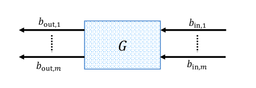
Figure 1: A quantum linear system.

$$\begin{split}&[\mathbf{a}_{j}(t),~{}\mathbf{a}_{k}(t)]=[\mathbf{a}_{j}^{\ast}(t),~{}\mathbf{a}_{k}^{\ast}(t)]=0,\;[\mathbf{a}_{j}(t),~{}\mathbf{a}_{k}^{\ast}(t)]=\delta_{jk},\ \ \ \forall j,k=1,\ldots,n,\forall t\in\mathbb{R}.\end{split}$$ (5)

Let $\mathbf{a}=[\mathbf{a}_{1}~{}\cdots~{}\mathbf{a}_{n}]^{\top}$ and $\breve{\mathbf{a}}=[\mathbf{a}^{\top}~{}(\mathbf{a}^{\#})^{\top}]^{\top}$ as introduced in the Notation part. Then Eq. (5) can be rewritten as

$$[\breve{\mathbf{a}}(t),\breve{\mathbf{a}}^{\dagger}(t)]=J_{n}.$$ (6)

The Hamiltonian of the quantum linear system is at most quadratic in terms of $\mathbf{a}$ and $\mathbf{a}^{\#}$, thus it is of the form

$$\mathbf{H}=\frac{1}{2}\breve{\mathbf{a}}^{\dagger}\Omega\breve{\mathbf{a}}+\breve{\mathbf{a}}^{\dagger}K\breve{v}+\breve{v}^{\dagger}K^{\dagger}\breve{\mathbf{a}},$$ (7)

where $\Omega=\Delta(\Omega_{-},\Omega_{+})$ is a Hermitian matrix with $\Omega_{-},\Omega_{+}\in\mathbb{C}^{n\times n}$, $K=\bigl{[}\begin{smallmatrix}K_{1}&K_{2}\\ K_{3}&K_{4}\end{smallmatrix}\bigr{]}\in\mathbb{C}^{2n\times 2l}$, and $\breve{v}\in\mathbb{C}^{2l}$ is a vector of classical signals used to model the laser or other classical signals that drive the system ([42, Eq. (20)], [2, Chapter 3], [9, Section 5.1.1], [30, Eq. (1)], [43, Eq. (C6)], [44, Eq. (9)]). For example, the quantum system can be a particle moving in a potential well whose potential can be controlled. In the literature of measurement-based quantum feedback control [5], $\breve{\mathbf{a}}^{\dagger}K\breve{v}+\breve{v}^{\dagger}K^{\dagger}\breve{\mathbf{a}}$ are often called the control Hamiltonian. For example, a quantum system can be measured and the measurement data can be processed by a classical controller that generates the classical control signal $v$ which is sent back to the quantum system to modulate its dynamics. The system is coupled to the input fields via the operator $\mathbf{L}=[C_{-}\ C_{+}]\breve{\mathbf{a}}$, with $C_{-},C_{+}\in\mathbb{C}^{m\times n}$. The input boson field $k$, $k=1,\ldots,m$, is described in terms of an annihilation operator $\mathbf{b}_{\mathrm{in},k}(t)$ and a creation operator $\mathbf{b}_{\mathrm{in},k}^{\ast}(t)$, which is the adjoint operator of $\mathbf{b}_{\mathrm{in},k}(t)$. If there are no photons in an input channel, this input channel is in the vacuum state denoted $\ket{\Phi_{0}}$. Annihilation and creation operators of these free traveling fields satisfy the following commutation relations

$$\mathbf{b}_{\mathrm{in},j}(t)\ket{\Phi_{0}}=0,\ [\mathbf{b}_{\mathrm{in},j}(t),\mathbf{b}_{\mathrm{in},k}(r)]=[\mathbf{b}_{\mathrm{in},j}^{\ast}(t),\mathbf{b}_{\mathrm{in},k}^{\ast}(r)]=0,$$ (8)

$$[\mathbf{b}_{\mathrm{in},j}(t),\mathbf{b}_{\mathrm{in},k}^{\ast}(r)]=\delta_{jk}\delta(t-r),\ \ \forall j,k=1,\ldots,m,\ t,r\in\mathbb{R}.$$

Eq. (8) can be re-written in the vector form

$$\mathbf{b}_{\mathrm{in}}(t)\ket{\Phi_{0}}=0,\ \;[\breve{\mathbf{b}}_{\rm in}(t),\ \breve{\mathbf{b}}^{\dagger}_{\rm in}(r)]=\delta(t-r)J_{m},\ t,r\in\mathbb{R}.$$ (9)

Before interacting with the system, the input fields may pass through some static devices, for example beamsplitters and phase shifters. This is modeled by a unitary matrix $S\in\mathbb{C}^{m\times m}$. $S$ is often referred to as scattering matrix in the quantum optics literature.

The integrated input annihilation, creation, and gauge processes (counting processes) are given by

$$\mathbf{B}_{\rm in}(t)=\int_{t_{0}}^{t}\mathbf{b}_{\rm in}(r)dr,\ \ \mathbf{B}^{\#}(t)=\int_{t_{0}}^{t}\mathbf{b}_{\rm in}^{\#}(r)dr,\ \ \mathbf{\Lambda}_{\rm in}(t)=\int_{t_{0}}^{t}\mathbf{b}_{\rm in}^{\#}(r)\mathbf{b}_{\rm in}^{\top}(r)dr.$$ (10)

respectively, where $t_{0}$ is the initial time when the system and the input fields start interaction. In this article, the input fields are assumed to be canonical fields which satisfy the Itô table (1).

Table 1: Quantum Itô table

$\times$	$d\mathbf{B}_{{\rm in},l}(t)$	$d\mathbf{B}_{{\rm in},m}^{\ast}(t)$	$d\mathbf{\Lambda}_{{\rm in},lm}(t)$	$dt$
$d\mathbf{B}_{{\rm in},j}(t)$	0	$\delta_{jm}dt$	$\delta_{jl}d\mathbf{B}_{m}(t)$	0
$d\mathbf{B}_{{\rm in},j}^{\ast}(t)$	0	0	0	0
$d\mathbf{\Lambda}_{{\rm in},jk}(t)$	0	$\delta_{km}d\mathbf{B}_{{\rm in},j}^{\ast}(t)$	$\delta_{kl}d\mathbf{\Lambda}_{{\rm in},jm}(t)$	0
$dt$	0	0	0	0

In the Heisenberg picture, in terms of the triple of parameters $(S,\mathbf{L},\mathbf{H})$ introduced above, the dynamics of the open quantum system in 1 is governed by a unitary operator $\mathbf{U}(t)$ that is the solution to the following Itô quantum stochastic differential equation (QSDE), first developed by [45],

$$d\mathbf{U}(t) =\;\bigm{\{}-(\mathbf{L}^{\dagger}\mathbf{L}/2+\imath\mathbf{H})dt+d\mathbf{B}_{\rm in}^{\dagger}(t)\mathbf{L}$$ (11)

$$\hskip 30.1388pt-\mathbf{L}^{\dagger}Sd\mathbf{B}_{\rm in}(t)+\mathrm{Tr}[(S-I)d\mathbf{\Lambda}_{\rm in}^{\top}(t)]\bigm{\}}\mathbf{U}(t),\ \ t\geq t_{0}$$

with the initial condition $U(t_{0})=I$ (the identity operator). Let $\mathbf{X}$ be a system operator. In the Heisenberg picture, we have

$$\mathbf{X}(t)=\mathbf{U}^{\ast}(t)(\mathbf{X}\otimes I_{\mathrm{field}})\mathbf{U}(t),\ \ t\geq t_{0}.$$ (12)

According to Eq. (11) and by quantum Itô calculus, we have

$$d\mathbf{X}(t)= \;\mathcal{L}_{\mathbf{L},\mathbf{H}}(\mathbf{X}(t))dt+d\mathbf{B}_{\rm in}^{\dagger}(t)S^{\dagger}[\mathbf{X}(t),\mathbf{L}(t)]$$ (13)

$$\;+[\mathbf{L}^{\dagger}(t),\mathbf{X}(t)]Sd\mathbf{B}_{\rm in}(t)+\mathrm{Tr}[(S^{\dagger}\mathbf{X}(t)S-\mathbf{X}(t))d\mathbf{\Lambda}_{\rm in}^{\top}(t)],$$

where the superoperator

$$\mathcal{L}_{\mathbf{L},\mathbf{H}}(X(t))\triangleq-\imath[\mathbf{X}(t),\mathbf{H}(t)]+\frac{1}{2}\mathbf{L}^{\dagger}(t)[\mathbf{X}(t),\mathbf{L}(t)]+\frac{1}{2}[\mathbf{L}^{\dagger}(t),\mathbf{X}(t)]\mathbf{L}(t).$$ (14)

(Notice that even initially $X$ is an operator on the system’s state space, $X(t)$ is an operator on the state space of the joint system-field system).

On the other hand, after interaction, the integrated output annihilation operators and gauge processes

$$\mathbf{B}_{\mathrm{out}}(t)= \;\mathbf{U}^{\ast}(t)(I_{\mathrm{system}}\otimes\mathbf{B}_{\rm in}(t))\mathbf{U}(t),$$ (15)

$$\mathbf{\Lambda}_{\mathrm{out}}(t)= \;\mathbf{U}^{\ast}(t)(I_{\mathrm{system}}\otimes\mathbf{\Lambda}_{\rm in}(t))\mathbf{U}(t)$$

are generated, and their dynamical evolution is given by

$$d\mathbf{B}_{\mathrm{out}}(t)= \;\mathbf{L}(t)dt+Sd\mathbf{B}_{\rm in}(t),$$ (16)

$$d\mathbf{\Lambda}_{\mathrm{out}}(t)= \;\mathbf{L}^{\#}(t)\mathbf{L}^{\top}(t)dt+S^{\#}d\mathbf{B}_{\rm in}^{\#}(t)L^{\top}(t)$$

$$\;+\mathbf{L}^{\#}(t)d\mathbf{B}_{\rm in}^{\top}(t)S^{\top}(t)+S^{\#}d\mathbf{\Lambda}_{\rm in}(t)S^{\top}.$$

Remark 2.1

According to Eq. (9), the quantum Itô table is satisfied by the Bosonic fields that are in the vacuum state $\ket{\Phi_{0}}$. In quantum optics, the input $\mathbf{B}_{\rm in}$ may be of the from $d\mathbf{B}_{\rm in}(t)=w(t)dt+d\tilde{\mathbf{B}}_{\rm in}(t)$, where $w(t)$ can be an operator of another quantum linear system, and $\tilde{\mathbf{B}}_{\rm in}(t)$ is in the vacuum state [2, 46]. For example, $\mathbf{B}_{\rm in}$ may be the output of a quantum linear system $K$. In this case, in analogy to Eq. (16), $\mathbf{B}_{\rm in}(t)$ will be of the form $\mathbf{L}_{K}(t)dt+S_{K}d\mathbf{B}_{{\rm in},K}(t)$ with $\mathbf{L}_{K},S_{K},\mathbf{B}_{{\rm in},K}(t)$ being the coupling operator, scattering matrix and input filed for the quantum system $K$. Thus, $w(t)=\mathbf{L}_{K}(t)$ and $d\tilde{\mathbf{B}}_{\rm in}(t)=S_{K}d\mathbf{B}_{{\rm in},K}(t)$. More detail can be found in Section 8. The input field $d\mathbf{B}_{\rm in}(t)$ of the above form also satisfies the quantum Itô table. Moreover, as will be shown in Subsection 7.1, fields in continuous-mode single-photon states also satisfy the quantum Itô table. However, there do exist fields that do not satisfy the quantum Itô table. For example, the coherent state $\ket{\alpha}$ with $\alpha\neq 0$ to be introduced in Section 4 does not satisfy the quantum Itô table. In such cases, another quantum system, often referred to as a modulating filter may be designed which is driven by a vacuum field and generates the desired input fields. Consequently, by cascading the modulating filter and the original quantum system, the quantum Itô QSDE (11) still holds. The problem of generating various nonclassical quantum input field states with modulating filters has been discussed in [47, 48], and [49].

By means of Eqs. (13) and (16), it can be shown that the evolution of the quantum linear system is governed by a system of QSDEs

$$\dot{\breve{\mathbf{a}}}(t)= \;\mathcal{A}\breve{\mathbf{a}}(t)+\mathcal{E}\breve{v}(t)+\mathcal{B}\breve{\mathbf{b}}_{\rm in}(t),$$ (17)

$$\breve{\mathbf{b}}_{\mathrm{out}}(t)= \;\mathcal{C}\breve{\mathbf{a}}(t)+\mathcal{D}\breve{\mathbf{b}}_{\rm in}(t),\ \ t\geq t_{0},$$

where the constant system matrices are given by

$$\;\mathcal{D}=\Delta(S,0),~{}\mathcal{C}=\Delta(C_{-},\ C_{+}),~{}\mathcal{B}=-\mathcal{C}^{\flat}\mathcal{D},$$ (18)

$$\;\mathcal{A}=-\imath J_{n}\Omega-\frac{1}{2}\mathcal{C}^{\flat}\mathcal{C},\ \ \mathcal{E}=-\imath\left(J_{n}K+\mathbb{J}_{n}K^{\#}\left[\begin{array}[]{@{}cc@{}}0&I_{n}\\ I_{n}&0\end{array}\right]\right).$$

The form of the system Eq. (17) is often referred to as the quantum Langevin equation. It should be understood in the Itô form

$$d\breve{\mathbf{a}}(t)= \;\mathcal{A}\breve{\mathbf{a}}(t)dt+\mathcal{E}\breve{v}(t)dt+\mathcal{B}d\breve{\mathbf{B}}_{\rm in}(t),$$ (19)

$$d\breve{\mathbf{B}}_{\mathrm{out}}(t)= \;\mathcal{C}\breve{\mathbf{a}}(t)dt+\mathcal{D}d\breve{\mathbf{B}}_{\rm in}(t),\ \ t\geq t_{0},$$

Remark 2.2

Notice that $v(t)$ in system (17) is a classical signal, for example photocurrent. On the other hand, in the literature of quantum coherent feedback control, two quantum systems may directly couple to each other via some interaction Hamiltonian, where the involved signals are all quantum operators; see, e.g, [50, Figs. 8(b) and 16], [1, Eqs. (3.1) and (4.1)], [51, Section II.B], and [52, Fig. 3.1].

The constant system matrices in Eq. (18) are parametrized by the physical parameters $\Omega_{-},\Omega_{+},C_{-},C_{+},S$ and they satisfy the following physical realizability conditions

$${\mathcal{A}}+{\mathcal{A}}^{\flat}+{\mathcal{B}}{\mathcal{B}}^{\flat}= \;0,$$ (20)

$${\mathcal{B}}= \;-{\mathcal{C}}^{\flat}{\mathcal{D}}.$$

Remark 2.3

Broadly speaking, if its system parameters satisfy the physical realizability conditions (20), the system (17) can be physically realized by a genuine quantum-mechanical system. For example, the fundamental commutation relations are preserved during temporal evolution

$$[\breve{\mathbf{a}}(t),~{}\breve{\mathbf{a}}^{\dagger}(t)]= \;[\breve{\mathbf{a}}(t_{0}),~{}\breve{\mathbf{a}}^{\dagger}(t_{0})],~{}~{}~{}t\geq t_{0},$$ (21)

$$[\breve{\mathbf{a}}(t),\breve{\mathbf{b}}_{\mathrm{out}}^{\dagger}(r)]= \;0,~{}t_{0}\leq r<t.$$

The problem of physical realization of quantum linear systems was first addressed in [46] and [53]. A comprehensive study of physical realization of quantum linear systems is nicely summarized in [9, Chapter 3], see also [54], [55], [56] and [40, Sections 2.4 and 3]. Further development can be found in [57, 58]. The problem of physical realization of quantum nonlinear systems has been studied in [59] and [60]. This physical realization theory for quantum systems can be regarded as an generalization of the network analysis and synthesis theory for classical systems [61].

As in the classical linear systems theory, the impulse response function from $\breve{\mathbf{b}}_{\rm in}(t)$ to $\breve{\mathbf{b}}_{\rm out}(t)$ is defined as

$$g_{G}(t)\triangleq\left\{\begin{array}[]{ll}\delta(t){\cal D}-{\cal C}e^{{\cal A}t}\cal{C}^{\flat}{\cal D},&t\geq 0,\\ 0,&t<0.\end{array}\right.$$ (22)

Define matrix functions

$$g_{G^{-}}(t)\triangleq \;\left\{\begin{array}[]{@{}ll@{}}\delta(t)S-[\begin{array}[]{@{}ll@{}}C_{-}&C_{+}\end{array}]e^{{\mathcal{A}}t}\left[\begin{array}[]{@{}c@{}}C_{-}^{\dagger}\\ -C_{+}^{\dagger}\end{array}\right]S,&t\geq 0,\\ 0,&t<0,\end{array}\right.$$ (23)

$$\ g_{G^{+}}(t)\triangleq \;\left\{\begin{array}[]{@{}ll@{}}-[\begin{array}[]{@{}ll@{}}C_{-}&C_{+}\end{array}]e^{{\mathcal{A}}t}\left[\begin{array}[]{@{}c@{}}-C_{+}^{T}\\ C_{-}^{T}\end{array}\right],&t\geq 0,\\ 0,&t<0.\end{array}\right.$$

It is easy to show that the impulse response function $g_{G}(t)$ defined in Eq. (22) has a nice structure of the form

$$g_{G}(t)=\Delta\left(g_{G^{-}}(t),g_{G^{+}}(t)\right).$$ (24)

Define the bilateral Laplace transform [62, Chapter 10]

$$\mathbf{a}[s]\triangleq\int_{-\infty}^{\infty}e^{-st}\mathbf{a}(t)dt$$ (25)

Conjugating both sides of Eq. (25) yields

$$\mathbf{a}[s]^{\#}=\int_{-\infty}^{\infty}e^{-s^{\ast}t}\mathbf{a}^{\#}(t)dt$$ (26)

Denote

$$\mathbf{a}^{\#}[s]\equiv\mathbf{a}[s^{\ast}]^{\#},\ \ \ \breve{\mathbf{a}}[s]\equiv\left[\begin{array}[]{@{}c@{}}\mathbf{a}[s]\\ \mathbf{a}^{\#}[s]\end{array}\right].$$ (27)

Then

$$\breve{\mathbf{a}}[s]=\int_{-\infty}^{\infty}e^{-st}\breve{\mathbf{a}}(t)dt.$$ (28)

Using similar definitions and notations for other operators or functions, the transfer function from $f\breve{\mathbf{b}}_{\rm in}[s]$ to $\breve{\mathbf{b}}_{\rm out}[s]$ is

$$\Xi_{G}[s]=\mathcal{C}(sI-\mathcal{A})^{-1}\mathcal{B}+\mathcal{D}.$$ (29)

Remark 2.4

The notation in Eq. (27) is consistent with that in [41] and [9, Section 2.3.3], but is slightly different from that in [50]. For example, $b_{2}^{\ast}(s^{\ast})$ in [50, Eq. (3)] is $\mathbf{b}_{\mathrm{in},2}^{\ast}[s]$ in our notation. The same is true for the other operators. Also, in this article we use $[s]$ to indicate the frequency domain and $(t)$ to indicate the time domain, as have been adopted in [63, 64] and [65].

Due to the structure of the impulse response function (24), the transfer function $\Xi_{G}[s]$ defined in Eq. (29) enjoys the following nice properties

$$\Xi_{G}[-s^{\ast}]^{\flat}\Xi_{G}[s]=I_{2m},~{}~{}\forall s\in\mathbb{C},$$ (30)

and

$$\Xi_{G}[\imath\omega]^{\flat}\Xi_{G}[\imath\omega]=\Xi_{G}[\imath\omega]\Xi_{G}[\imath\omega]^{\flat}=I_{2m},~{}~{}\forall\omega\in\mathbb{R}.$$ (31)

(A derivation of Eq. (30) can be seen in [41, Section VI.H], and Eq. (31) follows Eq. (30) by setting $s=\imath\omega$.)

If $C_{+}=0$, $\Omega_{+}=0$, $K_{2}=0$ and $K_{3}=0$, the resulting quantum linear system is said to be passive [51, 56, 9, 65]. Specifically, the Itô QSDEs for a passive linear quantum system are

$$\begin{split}d\mathbf{a}(t)=&\;A\mathbf{a}(t)dt+Ev(t)dt+Bd\mathbf{B}_{\rm in}(t),\\ d\mathbf{B}_{\mathrm{out}}(t)=&\;C\mathbf{a}(t)dt+Dd\mathbf{B}_{\rm in}(t),\ \ t\geq t_{0},\end{split}$$ (32)

where

$$A=-\imath\Omega_{-}-\frac{1}{2}C_{-}^{\dagger}C_{-},\ \ E=-\imath(K_{1}+K_{4}^{\#}),\ \ B=-C_{-}^{\dagger}S,\ C=C_{-},\ D=S.$$

In the passive case, the physical realizability conditions (20) reduce to

$$A+A^{\dagger}+BB^{\dagger}=0,~{}B=-C^{\dagger}S.$$ (33)

Moreover, in the passive case, $\Xi_{G^{+}}[s]\equiv 0$ and

$$\Xi_{G^{-}}[s]=S-C_{-}(sI+\imath\Omega_{-}+\frac{1}{2}C_{-}^{\dagger}C_{-})^{-1}C_{-}^{\dagger}S.$$ (34)

In other words, the dynamics of a quantum linear passive system are completely characterized by its annihilation operators. Finally, it can be easily verified that for a quantum linear passive system, the following holds

$$\Xi_{G^{-}}[\imath\omega]^{\dagger}\Xi_{G^{-}}[\imath\omega]\equiv I_{m},~{}~{}~{}\forall\omega\in\mathbb{R}.$$ (35)

As a result, a quantum linear passive system does not change the amplitude of the input signal, but modifies its phase.

Besides the annihilation–creation operator representation (17), a quantum linear system can also be described in the (real) quadrature operator representation. For a positive integer $k$, define the unitary matrix

$$V_{k}\triangleq\frac{1}{\sqrt{2}}\left[\begin{array}[]{@{}cc@{}}I_{k}&I_{k}\\ -\imath I_{k}&\imath I_{k}\end{array}\right].$$ (36)

The following unitary transformations

$$\left[\begin{array}[]{@{}c@{}}\mathbf{q}\\ \mathbf{p}\end{array}\right]\equiv \mathbf{x}\triangleq V_{n}\breve{\mathbf{a}},\ \ u\triangleq V_{l}\breve{v},$$ (37)

$$\left[\begin{array}[]{@{}c@{}}\mathbf{q}_{\mathrm{in}}\\ \mathbf{p}_{\mathrm{in}}\end{array}\right]\equiv \mathbf{u}\triangleq V_{m}\breve{\mathbf{b}},\ \left[\begin{array}[]{@{}c@{}}\mathbf{q}_{\mathrm{out}}\\ \mathbf{p}_{\mathrm{out}}\end{array}\right]\equiv\mathbf{y}\triangleq V_{m}\breve{\mathbf{b}}_{\mathrm{out}},$$

generate real quadrature operators of the system, the classical signal and the fields. The counterparts of the commutation relations (6) and (8) are

$$[\mathbf{x},\mathbf{x}^{\top}]=\imath\mathbb{J}_{n},$$ (38)

and

$$[\mathbf{u}(t),\ \mathbf{u}^{\top}(r)]=\imath\delta(t-r)\mathbb{J}_{m},\ t,r\in\mathbb{R}$$ (39)

respectively.

Remark 2.5

In some works, for example [46, 33], and [9], the transformations $\mathbf{q}=\mathbf{a}+\mathbf{a}^{\#}$, and $\mathbf{p}=-\imath\mathbf{a}+\imath\mathbf{a}^{\#}$ are adopted. In this case, Eq. (38) becomes

$$[\mathbf{x},\mathbf{x}^{\top}]=2\imath\mathbb{J}_{n}.$$ (40)

In terms of unitary transformations in Eq. (37), the coupling operator $\mathbf{L}$ and the Hamiltonian $\mathbf{H}$ are transformed to

$$\mathbf{L}= \;\Lambda\mathbf{x},$$ (41)

$$\mathbf{H}= \;\frac{1}{2}\mathbf{x}^{\top}\mathbb{H}\mathbf{x}+\mathbf{x}^{\top}\mathbb{K}u+u^{\top}\mathbb{K}^{\dagger}\mathbf{x},$$

where

$$\Lambda=[C_{-}\ C_{+}]V_{n}^{\dagger},\ \ \mathbb{H}=V_{n}\Omega V_{n}^{\dagger},\ \ \mathbb{K}=V_{n}KV_{l}^{\dagger}.$$ (42)

The QSDEs that describe the dynamics of the linear quantum system in 1 in the real quadrature operator representation are the following:

$$\dot{\mathbf{x}}= \;\mathbb{A}\mathbf{x}+\mathbb{E}u+\mathbb{B}\mathbf{u},$$ (43)

$$\mathbf{y}= \;\mathbb{C}\mathbf{x}+\mathbb{D}\mathbf{u},$$

where

$$\mathbb{D}= \;V_{m}\mathcal{D}V_{m}^{\dagger}=\left[\begin{array}[]{@{}cc@{}}\mathrm{Re}(S)&-\mathrm{Im}(S)\\ \mathrm{Im}(S)&\mathrm{Re}(S)\end{array}\right],$$ (44)

$$\mathbb{C}= \;V_{m}\mathcal{C}V_{n}^{\dagger}=\left[\begin{array}[]{@{}ll@{}}\mathrm{Re}(C_{-}+C_{+})&\mathrm{Im}(-C_{-}+C_{+})\\ \mathrm{Im}(C_{-}+C_{+})&\mathrm{Re}(C_{-}-C_{+})\end{array}\right],$$

$$\mathbb{B}= \;V_{n}\mathcal{B}V_{m}^{\dagger}=-\mathbb{C}^{\sharp}\mathbb{D},$$

$$\mathbb{A}= \;V_{n}\mathcal{A}V_{n}^{\dagger}=\mathbb{J}_{n}\mathbb{H}-\frac{1}{2}\mathbb{C}^{\sharp}\mathbb{C},$$

$$\mathbb{E}= \;\mathbb{J}_{n}(\mathbb{K}+\mathbb{K}^{\#}).$$

It is easy to verify that $\mathbb{D}\mathbb{D}^{\sharp}=I_{2m}$. Define Itô increments

$$d\mathbf{Q}_{\rm in}(t)=\int_{t}^{t+dt}\mathbf{q}_{\rm in}(r)dr,\ \ d\mathbf{P}_{\rm in}(t)=\int_{t}^{t+dt}\mathbf{p}_{\rm in}(r)dr,$$ (45)

$$d\mathbf{Q}_{\rm out}(t)=\int_{t}^{t+dt}\mathbf{q}_{\rm out}(r)dr,\ \ d\mathbf{P}_{\rm out}(t)=\int_{t}^{t+dt}\mathbf{p}_{\rm out}(r)dr.$$

And denote

$$\mathcal{U}(t)=\left[\begin{array}[]{@{}c@{}}\mathbf{Q}_{\rm in}(t)\\ \mathbf{P}_{\rm in}(t)\end{array}\right],\ \ \ \mathcal{Y}(t)=\left[\begin{array}[]{@{}c@{}}\mathbf{Q}_{\rm out}(t)\\ \mathbf{P}_{\rm out}(t)\end{array}\right].$$ (46)

Then system (43) can be re-written as

$$d\mathbf{x}(t)= \;\mathbb{A}\mathbf{x}(t)dt+\mathbb{E}udt+\mathbb{B}d\mathcal{U}(t),$$ (47)

$$d\mathcal{Y}(t)= \;\mathbb{C}\mathbf{x}(t)dt+\mathbb{D}d\mathcal{U}(t)$$

3 Hurwitz stability, controllability and observability

Hurwitz stability, controllability and observability are fundamental concepts of classical linear systems [66, 67, 68, 69]. Interestingly, these concepts can naturally be generalized to linear quantum systems. In the following discussions of this section, we assume the classical signal $u=0$ in Eq. (43).

If we take expectation on both sides of Eq. (43) with respect to the initial joint system-field state we get a classical linear system

$$\frac{d\langle\mathbf{x}(t)\rangle}{dt} = \mathbb{A}\langle\mathbf{x}(t)\rangle+\mathbb{B}\langle\mathbf{u}(t)\rangle,$$ (48)

$$\langle\mathbf{y}(t)\rangle = \mathbb{C}\langle\mathbf{x}(t)\rangle+\mathbb{D}\langle\mathbf{u}(t)\rangle.$$

Thus we can define controllability, observability, and Hurwitz stability for the quantum linear system (43) using those for the classical linear system (48).

Definition 3.1

The quantum linear system (43) is said to be Hurwitz stable (resp. controllable, observable) if the corresponding classical linear system (48) is Hurwitz stable (resp. controllable, observable).

Decoherence-free subsystems for linear quantum systems have recently been studied in e.g., [70, 22, 24, 25, 56, 71, 72, 73] and [65] and references therein. It turns out that decoherence-free subsystems are uncontrollable/unobservable subspaces in the linear quantum systems setting.

Definition 3.2 ([65, Definition 2.1])

The linear span of the system variables related to the uncontrollable/unobservable subspace of a linear quantum system is called its decoherence-free subsystem (DFS).

In quantum information science, decoherence-free subspaces are widely used for protecing ueful quantum informaiton; see for example [74] and [75]. The relation between decoherence-free subsystems and decoherence-free subspaces are discussed in [76].

In principle, an observable can be measured. However, the measurement may perturb the future evolution of this observable; this is the so-called quantum measurement back-action. Interestingly, sometimes one can engineer a quantum system so that measurement will not affect the evolution of the desired observable. Observables having this property are referred to as quantum non-demolition (QND) variables; see e.g., [77, 78, 79, 80, 25, 31] and [65].

Definition 3.3

An observable $\mathbf{F}$ is called a continuous-time QND variable if

$$[\mathbf{F}(t_{1}),\mathbf{F}(t_{2})]=0$$ (49)

for all time instants $t_{1},t_{2}\in\mathbb{R}^{+}$.

A natural extension of the notion of a QND variable is the following concept [80].

Definition 3.4 ([80]; [65, Definition 2.3])

The span of a set of observables $\mathbf{F}_{i}$, $i=1,\ldots,r$, is called a quantum mechanics-free subsystem (QMFS) if

$$[\mathbf{F}_{i}(t_{1}),\mathbf{F}_{j}(t_{2})]=0$$ (50)

for all time instants $t_{1},t_{2}\in\mathbb{R}^{+}$, and $i,j=1,\ldots,r$.

QND variables and QMFS subsystems are $\boldsymbol{p}_{h}$ in the Kalman canonical form of a quantum linear system; see Theorem 6.1 below.

Examples of physical realization of QMFS subsystems can be found in [31] and [65, Example 5.2].

The transfer function of the quantum linear system (43) from $\mathbf{u}$ to $\mathbf{y}$ is

$$\Xi_{\mathbf{u}\to{\mathbf{y}}}[s]=\mathbb{D}-\mathbb{C}(sI-\mathbb{A})^{-1}\mathbb{B}.$$ (51)

The transfer function relates the overall input $\mathbf{u}$ to the overall output $\mathbf{y}$. However, in many applications, we are interested in a particular subvector $\mathbf{u}^{\prime}$ of the input vector $\mathbf{u}$ and a particular subvector $\mathbf{y}^{\prime}$ of the output vector $\mathbf{y}$. This motivates us to introduce the following concept.

Definition 3.5 ([65, Definition 2.4])

For the linear quantum system (43), let $\Xi_{\mathbf{u}^{\prime}\to{\mathbf{y}}^{\prime}}[s]$ be the transfer function from a subvector $\mathbf{u}^{\prime}$ of the input vector $\mathbf{u}$ to a subvector $\mathbf{y}^{\prime}$ of the output vector $\mathbf{y}$. We say that system (43) realizes the back-action evasion (BAE) measurement of the output $\mathbf{y}^{\prime}$ with respect to the input $\mathbf{u}^{\prime}$ if $\Xi_{\mathbf{u}^{\prime}\to{\mathbf{y}}^{\prime}}[s]=0$ for all $s$.

More discussions on BAE measurements can be found in, e.g., [79, 19, 81, 25, 27, 82, 83], and the references therein.

We shall see that all of these notions can be nicely revealed by the Kalman decomposition of a linear quantum system, see Section 6.

4 Quantum Gaussian states

In this section, quantum Gaussian states are briefly introduced. More discussions can be found in, e.g., [2, 84, 42, 44, 85, 5, 86, 87, 64, 9, 88, 89, 90, 91] and references therein.

4.1 An introduction

Define the displacement operator

$$\mathbf{D}(\alpha)\triangleq\exp(\breve{\mathbf{a}}^{\dagger}J_{n}\breve{\alpha}),\ \ \forall\alpha\in\mathbb{C}^{n}.$$ (52)

Define the counterpart of $\breve{\alpha}$ in the real domain,

$$\beta=V_{n}\breve{\alpha}\in\mathbb{R}^{2n},$$ (53)

where $V_{n}$ is the unitary matrix defined in Eq. (36). Then the displacement operator defined in Eq. (52) can be re-written as

$$\mathbf{D}(\alpha)=\exp(\imath\mathbf{x}^{\top}\mathbb{J}_{n}\beta).$$ (54)

Given a density matrix $\rho$ of a quantum linear system, define its quantum characteristic function to be

$$\chi_{\rho}\triangleq\mathrm{Tr}[\rho\mathbf{D}(\alpha)].$$ (55)

For Gaussian states, we have, [85, Eq. (3.1)],

$$\chi_{\rho}=\exp\left(-\imath\mu^{\top}\mathbb{J}_{n}\beta-\frac{1}{2}\beta^{\top}\mathbb{V}\beta\right),$$ (56)

where

$$\mu= \;\mathrm{Tr}[\rho\mathbf{x}]\in\mathbb{R}^{2n},$$ (57)

$$\mathbb{V}= \;\frac{1}{2}\mathrm{Tr}\{\rho[(\mathbf{x}_{t}-\mu)(\mathbf{x}_{t}-\mu)^{\top}+((\mathbf{x}_{t}-\mu)(\mathbf{x}_{t}-\mu)^{\top}]^{\top}]\}\in\mathbb{R}^{2n\times 2n}.$$

are the mean and covariance, respectively. Define the complex domain counterpart of $\mu$ and $\mathbb{V}$ to be

$$\breve{\gamma}\triangleq \;V_{n}^{\dagger}\mu,$$ (58)

$$\Pi\triangleq \;V_{n}^{\dagger}\mathbb{V}V_{n}.$$

Then the quantum characteristic function in Eq. (56) can be re-written as

$$\chi_{\rho}=\exp\left(-\breve{\gamma}^{\dagger}J_{n}\breve{\alpha}-\frac{1}{2}\breve{\alpha}^{\dagger}\Pi\breve{\alpha}\right),$$ (59)

Moreover, for $\rho$ to be a Gaussian state of a quantum linear system, it is required that, [85, Theorem 3.1],

$$\mathbb{V} \geq \pm\frac{\imath}{2}\mathbb{J}_{n};$$ (60)

or equivalently,

$$\Pi \geq \pm\frac{1}{2}J_{n}.$$ (61)

In terms of the characteristic function $\chi_{\rho}$ defined in Eq. (55), we can define the Wigner function via the multi-dimensional Fourier transform

$$W_{\rho}(\mathrm{w})=\frac{1}{\sqrt{(2\pi)^{2n}}}\int_{\mathbb{R}^{2n}}\exp(-\imath\mathrm{w}^{\top}\mathbb{J}\beta)\mathrm{Tr}[\rho\exp(\imath\mathbf{x}^{\top}\mathbb{J}_{n}\beta)]d\beta,\ \ \forall\mathrm{w}\in\mathbb{R}^{2n}.$$ (62)

In particular, if $\rho$ is a Gaussian state with the characteristic function in Eq. (56), the Wigner function is of the form

$$W_{\rho}(\mathrm{w})=\frac{1}{\sqrt{(2\pi)^{2n}\mathrm{det}(\mathbb{V})}}\exp\left(-\frac{1}{2}(\mathrm{w}-\mu)^{\top}\mathbb{V}^{-1}(\mathrm{w}-\mu)\right),$$ (63)

with the mean $\mu$ and covariance matrix $\mathbb{V}$ given in Eq. (57). In other words, a Gaussian state is uniquely determined by its first and second moments.

Example 4.1

When $n=1$ and the system state is the quantum vacuum state $\ket{0}$, then $\rho=\ket{0}\bra{0}$, and

$$\mu=\mathrm{Tr}(\rho\mathbf{x})=\left[\begin{array}[]{@{}c@{}}0\\ 0\end{array}\right],\ \ \mathrm{Tr}(\rho\mathbf{q}^{2})=\mathrm{Tr}(\rho\mathbf{p}^{2})=\frac{1}{2},\ \ \mathrm{Tr}(\rho\mathbf{p}\mathbf{q})=-\frac{\imath}{2}.$$ (64)

The covariance matrix $\mathbb{V}$ in Eq. (57) becomes

$$\mathbb{V} = \frac{1}{2}\left[\begin{array}[]{@{}ll@{}}1&0\\ 0&1\end{array}\right].$$ (67)

Thus,

$$\mathbb{V}\pm\frac{\imath}{2}\mathbb{J}_{n}=\frac{1}{2}\left[\begin{array}[]{@{}ll@{}}1&\pm\imath\\ \mp\imath&1\end{array}\right]\geq 0,$$ (68)

which verifies Eq. (60). Moreover, the Wigner function (63) is now

$$W_{\rho}(w)=\frac{1}{\pi}\exp\left(-\frac{1}{2}w^{\top}w\right).$$ (69)

Finally, from Eq. (64) we have

$$\sqrt{\mathrm{Tr}(\rho\mathbf{q}^{2})}\sqrt{\mathrm{Tr}(\rho\mathbf{p}^{2})}=\frac{1}{2}.$$ (70)

For any state $\rho$ and observables $\mathbf{X}$ and $\mathbf{Y}$, the Heisenberg uncertainty relation is

$$\sqrt{\mathrm{Tr}(\rho\mathbf{X}^{2})-(\mathrm{Tr}(\rho\mathbf{X}))^{2}}\sqrt{\mathrm{Tr}(\rho\mathbf{Y}^{2})-(\mathrm{Tr}(\rho\mathbf{Y}))^{2}}\geq\frac{1}{2}|\mathrm{Tr}\left(\rho[\mathbf{X},\mathbf{Y}]\right)|.$$ (71)

According to Eq. (70), the vacuum state $\ket{0}$ saturates the Heisenberg uncertainty relation (71) when $\mathbf{X}=\mathbf{q}$ and $\mathbf{Y}=\mathbf{p}$. In the literature, states saturating the Heisenberg uncertainty relation (71) are often called minimum uncertainty states. For example, a special type of Gaussian states, coherent states, defined as

$$\ket{\alpha}\triangleq e^{-\frac{|\alpha|^{2}}{2}}\sum_{k=0}^{\infty}\frac{\alpha^{k}}{\sqrt{k!}}\ket{k},\ \ \alpha\in\mathbb{C},$$ (72)

are minimum uncertainty states as Eq. (71) is saturated when $\mathbf{X}=\mathbf{q}$ and $\mathbf{Y}=\mathbf{p}$.

Example 4.2

In this example, we show that the vacuum state $\ket{0}$ is a Gaussian state. For simplicity, we look at the single-oscillator case ($n=1$). In this case, the displacement operator $\mathbf{D}(\alpha)$ defined in Eq. (52) becomes

$$\mathbf{D}(\alpha)=\exp(\alpha\mathbf{a}^{\ast}-\alpha^{\ast}\mathbf{a}).$$ (73)

If two operators $\mathbf{A}$ and $\mathbf{B}$ satisfy $[\mathbf{A},[\mathbf{A},\mathbf{B}]]=[\mathbf{B},[\mathbf{A},\mathbf{B}]]=0$, then the Baker-Campbell-Hausdorff formula is

$$e^{\mathbf{A}+\mathbf{B}}=e^{\mathbf{A}}e^{\mathbf{B}}e^{-\frac{1}{2}[\mathbf{A},\mathbf{B}]}=e^{\mathbf{B}}e^{\mathbf{A}}e^{\frac{1}{2}[\mathbf{A},\mathbf{B}]}.$$ (74)

Therefore,

$$\mathbf{D}(\alpha)=e^{\alpha\mathbf{a}^{\ast}}e^{-\alpha^{\ast}\mathbf{a}}e^{-\frac{|\alpha|^{2}}{2}}.$$ (75)

As

$$e^{\alpha\mathbf{a}^{\ast}}e^{-\alpha^{\ast}\mathbf{a}}\ket{0}=e^{\alpha\mathbf{a}^{\ast}}\ket{0}=\sum_{k=0}^{\infty}\frac{\alpha^{k}}{\sqrt{k!}}\ket{k},$$ (76)

we have

$$\mathbf{D}(\alpha)\ket{0}=e^{-\frac{|\alpha|^{2}}{2}}\sum_{k=0}^{\infty}\frac{\alpha^{k}}{\sqrt{k!}}\ket{k}=\ket{\alpha}.$$ (77)

Consequently, the characteristic function for the vacuum state $\ket{0}$ is

$$\chi=\braket{0}{\mathbf{D}(\alpha)}{0}=e^{-\frac{|\alpha|^{2}}{2}},$$ (78)

which is of the form Eq. (59) with

$$\gamma=0,\ \ \Pi=\frac{1}{2}\left[\begin{array}[]{@{}ll@{}}1&0\\ 0&1\end{array}\right].$$ (79)

Clearly, $\Pi$ derived above satisfies the inequality (61), hence the vacuum state $\ket{0}$ is a Gaussian state.

In [92], [9, Section 2.7] and [64], another form of characteristic functions is defined for a Gaussian system state $\rho$, which is

$$\mathrm{Tr}[\rho\exp(i\breve{z}^{\dagger}\breve{\mathbf{a}})]=\exp(\imath\breve{z}^{\dagger}\breve{\beta}-\frac{1}{2}\breve{z}^{\dagger}\Sigma\breve{z}),~{}~{}\forall z\in\mathbb{C}^{n},$$ (80)

where $\breve{\gamma}=\mathrm{Tr}[\rho\breve{\mathbf{a}}]$, and $\Sigma=\mathrm{Tr}[\rho(\breve{\mathbf{a}}-\breve{\gamma})(\breve{\mathbf{a}}-\breve{\gamma})^{\dagger}]$ is a non-negative Hermitian matrix. In general, $\Sigma$ has the form

$$\Sigma=\left[\begin{array}[]{@{}cc@{}}I_{n}+N^{T}&M\\ M^{\dagger}&N\end{array}\right].$$ (81)

In particular, the ground or vacuum state $\ket{0}$ is specified by $\gamma=0$ and $\Sigma=\left[\begin{array}[]{@{}cc@{}}I_{n}&0\\ 0&0_{n}\end{array}\right]$. Clearly,

$$\frac{1}{2}\Sigma\geq\frac{\imath}{2}J_{n}.$$ (82)

However, the following is not true:

$$\frac{1}{2}\Sigma\geq-\frac{\imath}{2}J_{n}.$$ (83)

Consequently, to be consistent with $\mathbb{V}$ for the real quadrature operator representation, it is better to use the covariance matrix $\Pi$ given in Eq. (58), instead of $\Sigma$ in Eq. (81).

4.2 Pure Gaussian state generation

Gaussian states are very useful resources in quantum signal processing, [93, 94, 95] and [84, 96]. Thus, the problem of Gaussian state generation has been studied intensively in the quantum control literature. In this subsection, we present one result for pure Gaussian state generation by means of environment engineering.

A Gaussian state is a pure state is the determinant of its associated covariance $\mathbb{V}$ satisfies $\det(\mathbb{V})=1/2^{2n}$, where $n$ is the number of the oscillators. The covariance matrix $\mathbb{V}$ of a pure Gaussian state can be decomposed as ([87, Eq. (16)]; [86, Eq. (2.18)])

$$\mathbb{V}=\frac{1}{2}\mathbb{S}\,\mathbb{S}^{\top},$$ (84)

where

$$\mathbb{S}=\left[\begin{array}[]{@{}cc@{}}Y^{-1/2}&0\\ XY^{-1/2}&Y^{1/2}\end{array}\right]$$ (85)

with $X=X^{\top}\in\mathbb{R}^{n}$ and $Y=Y^{\top}\in\mathbb{R}^{n}$ being positive definite. As $\mathbb{S}\mathbb{J}_{n}\mathbb{S}^{\top}=\mathbb{J}_{n}$, $\mathbb{S}$ is symplectic (See the Notation part). Let $Z=X+\imath Y$.

Theorem 4.1 ([87])

The pure Gaussian state associated with the covariance matrix $\mathbb{V}$ in Eq. (84) can be generated by the linear quantum system (43) if and only if

$$\mathbb{H}=\left[\begin{array}[]{@{}cc@{}}XRX+YRY-\Gamma Y^{-1}X-XY^{-1}\Gamma^{\top}&-XR+\Gamma Y^{-1}\\ -RX+Y^{-1}\Gamma^{\top}&R\end{array}\right].$$ (86)

and

$$\Lambda=P^{\top}[-Z\ \ I],$$ (87)

where $R=R^{\top}$, $\Gamma=-\Gamma^{\top}$, and the matrix pair $(P,Q)$ is controllable with $Q=-\imath RY+Y^{-1}\Gamma$.

The problem of Gaussian state generation by means of environment engineering has been studied insensitively by the quantum control community. Interest reader may refer to [9, Section 6.1] and further development [97, 98, 99, 89, 90, 91].

4.3 Skew information and information-theoretic uncertainty relation

In addition to Heisenberg’s uncertainty relation (71), an information-theoretic uncertainty relation was proposed in [100] based on skew information. In what follows, we use the notation in [100]. Given a density operator $\rho$ and an observable $\mathbf{X}$, the Wigner–Yanase skew information [101] is defined as

$$I(\rho,\mathbf{X})\triangleq-\frac{1}{2}\mathrm{Tr}([\sqrt{\rho},\mathbf{X}]^{2}).$$ (88)

Skew information was originally defined for Hamiltonians of closed (namely, isolated) quantum systems [101], and was later generalized to arbitrary observables of open quantum systems. Roughly speaking, $I(\rho,\mathbf{X})$ measures the quantum uncertainty of the observable $\mathbf{X}$ with respect to the density operator $\rho$.

The variance of $\mathbf{X}$ with respect to the density operator $\rho$ is

$$V(\rho,\mathbf{X})=\mathrm{Tr}(\rho\mathbf{X}^{2})-(\mathrm{Tr}(\rho\mathbf{X}))^{2}.$$ (89)

When the state is pure, it is easy to see that $I(\rho,\mathbf{X})=V(\rho,\mathbf{X})$. However, $I(\rho,\mathbf{X})\leq V(\rho,\mathbf{X})$ when the state is a mixed one. To quantify quantum uncertainty, the following quantity has been defined in [100]:

$$U(\rho,\mathbf{X})\triangleq\sqrt{V^{2}(\rho,\mathbf{X})-(V(\rho,\mathbf{X})-I(\rho,\mathbf{X}))^{2}}.$$ (90)

The information-theoretic uncertainty relation is [100, Eq. (2)]

$$U(\rho,\mathbf{X})U(\rho,\mathbf{Y})\geq\frac{1}{4}|\mathrm{Tr}(\rho[\mathbf{X},\mathbf{Y}])|^{2}.$$ (91)

Interestingly, it is proved in [102] that when $n=1$ for the single-mode oscillator case, all Gaussian states, pure or mixed, are minimum uncertainty states, i.e., states that saturate (91). On the other hand, minimum uncertainty states are Gaussian states. However, in general mixed Gaussian states do not saturate the Heisenberg’s uncertainty relation (71). In this sense, the information-theoretic uncertainty relation (91) better characterizes Gaussian states. More studies on quantum skew-information and information-theoretic uncertainty relation can be found in, e.g., [103, 104, 105, 106, 107, 108, 109, 110, 111, 112, 113, 102] and references therein.

5 Quantum Kalman filter

Simply speaking, a quantum filter describes the temporal evolution of an open quantum system under repeated measurement. A general form of quantum filters is first presented in Subsection 5.1, after that the quantum filter for linear quantum systems is given in Subsection 5.2, which is of the form of the Kalman filter for classical linear systems. Finally, an example is given in Subsection 5.3 for demonstration. In this section, it is assumed that $S=I_{m}$ and the initial time $t_{0}=0$.

5.1 Quantum filter

In this subsection, we present a quantum filter for open quantum systems.

By Eq. (37), we have

$${[\mathbf{q}_{\rm in}(t_{1}),\mathbf{q}^{\top}_{\rm in}(t_{2})]}= \;\frac{1}{2}[\mathbf{b}_{{\rm in}}(t_{1})+\mathbf{b}^{\#}_{{\rm in}}(t_{1}),\mathbf{b}^{\dagger}_{{\rm in}}(t_{2})+\mathbf{b}^{\top}_{{\rm in}}(t_{2})]$$ (92)

$$= \;\frac{1}{2}[\mathbf{b}_{\rm in}(t_{1}),\mathbf{b}^{\dagger}_{{\rm in}}(t_{2})]+\frac{1}{2}[\mathbf{b}^{\#}_{{\rm in}}(t_{1}),\mathbf{b}^{\top}_{{\rm in}}(t_{2})]$$

$$= \;\frac{1}{2}\delta(t_{1}-t_{2})I_{m}-\frac{1}{2}\delta(t_{1}-t_{2})I_{m}$$

$$= \;0.$$

According to Eq. (15),

$$\mathbf{q}_{{\rm out}}(t)=U(t)^{\ast}(I_{\mathrm{system}}\otimes\mathbf{q}_{{\rm in}}(t))U(t).$$ (93)

Moreover, the unitary operator $U(t)$ has the following property [114, Section 5.2]

$$U(t_{2})^{\ast}(I_{\mathrm{system}}\otimes\mathbf{q}_{{\rm in}}(t_{1}))U(t_{2})=U(t_{1})^{\ast}(I_{\mathrm{system}}\otimes\mathbf{q}_{{\rm in}}(t_{1}))U(t_{1}),\ \ \ t_{1}\leq t_{2}.$$ (94)

Consequently, $\mathbf{q}_{\rm out}(t)$ enjoys the self-non-demolition property:

$$[\mathbf{q}_{\rm out}(t_{1}),\mathbf{q}^{\top}_{\rm out}(t_{2})]=0,~{}~{}0\leq t_{1}\leq t_{2}.$$ (95)

Moreover, from Eqs. (21) and (94) the following non-demolition property can be derived:

$$[\mathbf{X}(t),\mathbf{q}_{\rm out}(r)^{\top}]=0,~{}~{}t_{0}\leq r\leq t.$$ (96)

It can be easily verified that the integrated quadrature operator $\mathbf{Q}_{\rm out}(t)$ defined in Eq. (45) also enjoys the self-non-demolition property (95) and non-demolition property (96). Due to the self-non-demolition property (95), $\{\mathbf{Q}_{\rm out}(r):0\leq r\leq t\}$ can be regarded as a classical stochastic process. (Strictly speaking, measuring $\mathbf{Q}_{\rm out}(t)$ gives rise to a classical stochastic process.) Moreover, due to the non-demolition property (96), $\mathbf{X}(t)$ lives in the $\sigma$-field generated by this classical stochastic process. Hence, it is meaningful to define the expectation of $\mathbf{X}(t)$ conditioned on this $\sigma$-field. We denote this conditional expectation by $E[\mathbf{X}(t)|\{\mathbf{Q}_{\rm out}(r):0\leq r\leq t\}]$. Then, one can define the conditional density operator $\rho_{\rm c}(t)$ by means of

$$\mathrm{Tr}(\rho_{\rm c}(t)\mathbf{X})=E[\mathbf{X}(t)|\{\mathbf{Q}_{\rm out}(r):0\leq r\leq t\}].$$ (97)

Clearly, $\rho_{\rm c}(0)$ is the initial joint system density matrix denoted $\rho_{\rm S}(0)$. The dynamics of the conditioned density operator is given by the stochastic master equation (SME) (also called quantum trajectories [115], [116])

$$d\rho_{\rm c}(t) =\;\mathcal{L}^{\star}_{\mathbf{L},\mathbf{H}}(\rho_{\rm c}(t))dt$$ (98)

$$+\{\mathbf{L}^{\top}\rho_{\rm c}(t)+\rho_{\rm c}(t)\mathbf{L}^{\dagger}-\mathrm{Tr}[\rho_{\rm c}(t)(\mathbf{L}^{\top}+\mathbf{L}^{\dagger})]\rho_{\rm c}(t)\}d\nu(t),$$

where

$$d\nu(t)\triangleq d\mathbf{Q}_{\rm out}(t)-\pi_{t}(\mathbf{L}+\mathbf{L}^{\#})dt$$ (99)

is an innovation process, and the superoperator

$$\mathcal{L}^{\star}_{\mathbf{L},\mathbf{H}}(\rho_{\rm c}(t))=-\imath[\mathbf{H},\rho_{\rm c}(t)]+\mathbf{L}^{\top}\rho_{\rm c}(t)\mathbf{L}^{\#}-\frac{1}{2}\mathbf{L}^{\dagger}\mathbf{L}\rho_{\rm c}(t)-\frac{1}{2}\rho_{\rm c}(t)\mathbf{L}^{\dagger}\mathbf{L}.$$ (100)

For a given system operator $\mathbf{X}$, define the conditioned mean vector

$$\pi_{t}(\mathbf{X})\triangleq\mathrm{Tr}(\rho_{\rm c}(t)\mathbf{X}).$$ (101)

It turns out that $\pi_{t}(\mathbf{X})$ is the solution to the Belavkin quantum filtering equation, which is a classical stochastic differential equation[117], [118]

$$d\pi_{t}(\mathbf{X}) =\;\pi_{t}(\mathcal{L}_{\mathbf{L},\mathbf{H}}(\mathbf{X}))dt$$ (102)

$$+[\pi_{t}(\mathbf{X}\mathbf{L}^{\top}+\mathbf{L}^{\dagger}\mathbf{X})-\pi_{t}(\mathbf{L}^{\top}+\mathbf{L}^{\dagger})\pi_{t}(\mathbf{X})]d\nu(t),$$

with the initial condition $\pi_{0}(\mathbf{X})=\mathrm{Tr}(\rho_{\rm S}(0)\mathbf{X})$, where $\mathcal{L}_{\mathbf{L},\mathbf{H}}(\mathbf{X})$ is the superoperator defined in Eq. (14).

Remark 5.1

In classical control systems theory, measurement noise is always supposed to be decoupled from the system dynamics. This is no longer true in the quantum regime. As shown by Eq. (98), measurement affects the dynamics of the system which is being monitored. This is often called measurement back-action. Moreover, Eq. (43) show linear dynamics of the system. However, its conditioned dynamics (98) is nonlinear. This is essentially different from classical linear dynamics.

Remark 5.2

The measurement used in this section is homodyne measurement. There are other types of quantum measurements used in quantum filtering and feedback control, for instance, heterodyne measurement, photodetection and general positive operator valued measurements (POVMs). The experimental realization of a real-time POVM measurement-based feedback control of the 2012 Nobel prize winning photon-box is described in [18] and [17]. A comprehensive study of quantum measurement and feedback control is presented in [114] and [5].

Finally, denote

$$\rho(t)\triangleq E[\rho_{\rm c}(t)].$$ (103)

Then the unconditioned system dynamics are given by the Lindblad master equation

$$d\rho(t)=\mathcal{L}^{\star}_{\mathbf{L},\mathbf{H}}(\rho(t))dt.$$ (104)

More discussions of quantum filters can be found in [117, 16, 119, 120, 121, 114, 122, 123, 124, 125, 126, 127, 128, 129, 130], and [5], among others.

5.2 Quantum Kalman filter

The above formulations hold for general open quantum systems, in this subsection we present their specific forms for linear quantum systems. In this case, the quantum filter consists of Eqs. (106) and (108) to be given below, which is in the same form of a classical Kalman filter.

Define the conditional covariance matrix

$$V_{t}\triangleq{\rm Tr}\left[\rho_{c}(t)\frac{(\mathbf{x}-\pi_{t}(\mathbf{x}))(\mathbf{x}-\pi_{t}(\mathbf{x}))^{\top}+((\mathbf{x}-\pi_{t}(\mathbf{x}))(\mathbf{x}-\pi_{t}(\mathbf{x}))^{\top})^{\top}}{2}\right].$$ (105)

Theorem 5.1

The quantum Kalman filter for the quantum linear system (43) is of the form

$$d\pi_{t}(\mathbf{x})=\mathbb{A}\pi_{t}(\mathbf{x})dt+\mathbb{E}udt+(V_{t}\mathbb{C}_{1}^{\top}+M)d\nu(t),$$ (106)

with the initial condition $\pi_{0}(\mathbf{x})={\rm Tr}\left[\rho_{{\rm S}}(0)\mathbf{x}\right]$, where the matrices

$$\mathbb{C}_{1}=[I_{m}\ \ 0_{m}]\mathbb{C},\ \ M=\frac{1}{\sqrt{2}}\mathbb{B}\left[\begin{array}[]{@{}c@{}}I_{m}\\ 0_{m}\end{array}\right],$$ (107)

and the conditional covariance matrix $V_{t}$ solves the following differential Riccati equation

$$\dot{V}_{t}=\mathbb{A}V_{t}+V_{t}\mathbb{A}^{\top}+\frac{1}{2}\mathbb{B}\mathbb{B}^{\top}-(V_{t}\mathbb{C}_{1}^{\top}+M)(V_{t}\mathbb{C}_{1}^{\top}+M)^{\top}.$$ (108)

The quantum Kalman filter appears very close to the Kalman filter for classical linear systems [67, 131, Chapter 3].

In what follows, a proof of Theorem 5.1 is given,

Proof of Theorem 5.1 1

Look at Eq. (106) first.

Step 0. Let $\mathbf{X}$, $\mathbf{Y}$ and $\mathbf{Z}$ be vectors of operators of dimension $l$, $m$, and $n$, respectively. Let $M\in\mathbb{C}^{m\times n}$. If the commutators $[a,b]\in\mathbb{C}$ where $a$ and $b$ are arbitrary elements of the vectors $\mathbf{X}$, $\mathbf{Y}$ and $\mathbf{Z}$. Then

$$[\mathbf{X},\mathbf{Y}^{\top}M\mathbf{Z}]=[\mathbf{X},\mathbf{Y}^{\top}]M\mathbf{Z}+[\mathbf{X},\mathbf{Z}^{\top}]M^{\top}\mathbf{Y}.$$ (109)

Step 1. Substituting the vector $\mathbf{x}(t)$ in Eq. (43) into Eq. (14) and using Eqs. (2) and (109) we get

$$\pi_{t}(-\imath[\mathbf{x}(t),\mathbf{H}(t)]+\frac{1}{2}\mathbf{L}^{\dagger}(t)[\mathbf{x}(t),\mathbf{L}(t)]+\frac{1}{2}[\mathbf{L}^{\dagger}(t),\mathbf{x}(t)]\mathbf{L}(t))$$ (110)

$$= \;\mathbb{J}_{n}\mathbb{H}\pi_{t}(\mathbf{x})+\mathbb{J}_{n}(\mathbb{K}+\mathbb{K}^{\#})u+\frac{1}{2\imath}\mathbb{J}_{n}(\Lambda^{\dagger}\Lambda-\Lambda^{\top}\Lambda^{\#})\pi_{t}(\mathbf{x})$$

$$= \;\left(\mathbb{J}_{n}\mathbb{H}-\frac{1}{2}\mathbb{C}^{\sharp}\mathbb{C}\right)\pi_{t}(\mathbf{x})+\mathbb{J}_{n}(\mathbb{K}+\mathbb{K}^{\#})u$$

$$= \;\mathbb{A}\pi_{t}(\mathbf{x})+\mathbb{E}u.$$

Step 2. By Eqs. (40) and (105), we have

$$V_{t}=\pi_{t}(\mathbf{x}\mathbf{x}^{\top})-\frac{\imath}{2}\mathbb{J}_{n}-\pi_{t}(\mathbf{x})\pi_{t}(\mathbf{x})^{\top}.$$ (111)

Step 3. Noticing that

$$\mathbf{L}^{\dagger}\mathbf{q}=\mathbf{q}\mathbf{x}^{\top}\Lambda^{\dagger}-\imath\left[\begin{array}[]{@{}cc@{}}\mathbf{0}&I\end{array}\right]\Lambda^{\dagger},$$ (112)

$$\mathbf{L}^{\dagger}\mathbf{p}=\mathbf{p}\mathbf{x}^{\top}\Lambda^{\dagger}+\imath\left[\begin{array}[]{@{}cc@{}}I&\mathbf{0}\end{array}\right]\Lambda^{\dagger},$$

we have

$$\mathbf{L}^{\dagger}\mathbf{x}=\mathbf{x}\mathbf{L}^{\dagger}-\imath\mathbb{J}_{n}\Lambda^{\dagger}.$$ (113)

Step 4. By Eqs. (111) and (113), we get

$$\pi_{t}(\mathbf{x}\mathbf{L}^{\top}+\mathbf{L}^{\dagger}\mathbf{x})-\pi_{t}(\mathbf{L}^{\top}+\mathbf{L}^{\dagger})\pi_{t}(\mathbf{x})$$ (114)

$$= \;\pi_{t}(\mathbf{x}\mathbf{x}^{\top})\Lambda^{\top}+\pi_{t}(\mathbf{x}\mathbf{L}^{\dagger}-\imath\mathbb{J}_{n}\Lambda^{\dagger})-\pi_{t}(\mathbf{L}^{\top}+\mathbf{L}^{\dagger})\pi_{t}(\mathbf{x})$$

$$= \;\pi_{t}(\mathbf{x}\mathbf{x}^{\top})(\Lambda^{\top}+\Lambda^{\dagger})-\imath\mathbb{J}_{n}\Lambda^{\dagger}-\pi_{t}(\mathbf{L}^{\top}+\mathbf{L}^{\dagger})\pi_{t}(\mathbf{x})$$

$$= \;(\langle\mathbf{x}\mathbf{x}^{\top}\rangle-\pi_{t}(\mathbf{x})\pi_{t}(\mathbf{x})^{\top})(\Lambda^{\top}+\Lambda^{\dagger})-\imath\mathbb{J}_{n}\Lambda^{\dagger}$$

$$= \;(V_{t}+\frac{\imath}{2}\mathbb{J}_{n})(\Lambda^{\top}+\Lambda^{\dagger})-\imath\mathbb{J}_{n}\Lambda^{\dagger}$$

$$= \;V_{t}(\Lambda^{\top}+\Lambda^{\dagger})+\frac{\imath}{2}\mathbb{J}_{n}(\Lambda^{\top}-\Lambda^{\dagger}),$$

where

$$\pi_{t}(\mathbf{L}^{\top}+\mathbf{L}^{\dagger})\pi_{t}(\mathbf{x})=\pi_{t}(\mathbf{x})\pi_{t}(\mathbf{L}^{\top}+\mathbf{L}^{\dagger})=\pi_{t}(\mathbf{x})\pi_{t}(\mathbf{x}^{\top})(\Lambda^{\top}+\Lambda^{\dagger})$$ (115)

has been used in the derivation.

Combining (110), (114) with (99), we have

$$d\pi_{t}(\mathbf{x})= (\mathbb{A}\pi_{t}(\mathbf{x})+\mathbb{E}u)dt+\left(V_{t}\mathbb{C}_{1}^{\top}+\frac{\imath}{2}\mathbb{J}_{n}(\Lambda^{\top}-\Lambda^{\dagger})\right)d\nu_{t}$$ (116)

$$= (\mathbb{A}\pi_{t}(\mathbf{x})+\mathbb{E}u)dt+(V_{t}\mathbb{C}_{1}^{\top}+M)d\nu_{t},$$

which is Eq. (106).

Next, we derive Eq. (108).

By Eqs. (97) and (105), we have

$$V_{t}= \;E\bigg{[}\frac{(\mathbf{x}_{t}-\pi_{t}(\mathbf{x}))(\mathbf{x}_{t}-\pi_{t}(\mathbf{x}))^{\top}+((\mathbf{x}_{t}-\pi_{t}(\mathbf{x}))(\mathbf{x}_{t}-\pi_{t}(\mathbf{x}))^{\top})^{\top}}{2}$$

$$\hskip 28.45274pt\bigg{|}\{\mathbf{Q}_{\rm out}(r):0\leq r\leq t\}\bigg{]}.$$ (117)

As a result, by the property of conditional expectation,

$$E[V(t)]$$

$$= E\left[\frac{(\mathbf{x}_{t}-\pi_{t}(\mathbf{x}))(\mathbf{x}_{t}-\pi_{t}(\mathbf{x}))^{\top}+((\mathbf{x}_{t}-\pi_{t}(\mathbf{x}))(\mathbf{x}_{t}-\pi_{t}(\mathbf{x}))^{\top})^{\top}}{2}\right]$$

$$= \mathrm{Tr}\left[\rho_{S\otimes F}(0)\frac{(\mathbf{x}_{t}-\pi_{t}(\mathbf{x}))(\mathbf{x}_{t}-\pi_{t}(\mathbf{x}))^{\top}+((\mathbf{x}_{t}-\pi_{t}(\mathbf{x}))(\mathbf{x}_{t}-\pi_{t}(\mathbf{x}))^{\top})^{\top}}{2}\right],$$

where $\rho_{S\otimes F}(0)$ is the initial joint system-field density matrix. By the following property of Gaussian random variables: $V(t)=E[V(t)]$ almost surely (a.s.), see e.g., [132, Chapter 10], we have

$$V_{t}={\rm Tr}\left[\rho_{{\rm S}\otimes{\rm F}}(0)\frac{(\mathbf{x}_{t}-\pi_{t}(\mathbf{x}))(\mathbf{x}_{t}-\pi_{t}(\mathbf{x}))^{\top}+((\mathbf{x}_{t}-\pi_{t}(\mathbf{x}))(\mathbf{x}_{t}-\pi_{t}(\mathbf{x}))^{\top})^{\top}}{2}\right].$$ (119)

For convenience, in the following, we denote $\langle\mathbf{X}\rangle=\mathrm{Tr}[\rho_{S\otimes F}(0)\mathbf{X}]$ for an operator $\mathbf{X}$.

Step 0. Differentiating $\langle(\mathbf{x}-\pi_{t}(\mathbf{x}))(\mathbf{x}-\pi_{t}(\mathbf{x}))^{\top}\rangle$ with respect to $t$, yields

$$d\left\langle(\mathbf{x}_{t}-\pi_{t}(\mathbf{x}))(\mathbf{x}_{t}-\pi_{t}(\mathbf{x}))^{\top}\right\rangle$$ (120)

$$= \langle d(\mathbf{x}_{t}-\pi_{t}(\mathbf{x}))(\mathbf{x}_{t}-\pi_{t}(\mathbf{x}))^{\top}\rangle+\langle(\mathbf{x}_{t}-\pi_{t}(\mathbf{x}))d(\mathbf{x}_{t}-\pi_{t}(\mathbf{x}))^{\top}\rangle$$

$$+\ \ \langle d(\mathbf{x}_{t}-\pi_{t}(\mathbf{x}))d(\mathbf{x}_{t}-\pi_{t}(\mathbf{x}))^{\top}\rangle.$$

According to Eqs. (43) and (116), we have

$$d(\mathbf{x}_{t}-\pi_{t}(\mathbf{x}))=\mathbb{A}(\mathbf{x}_{t}-\pi_{t}(\mathbf{x}))dt+\mathbb{B}d\mathbf{u}-(V_{t}\mathbb{C}_{1}^{\top}+M)d\nu_{t}.$$ (121)

Moreover, it can be easily checked that

$$\mathrm{Tr}[\rho_{\rm S\otimes F}(0)\mathbb{B}d\mathbf{u}d\nu_{t}^{\top}] =-\imath\mathbb{J}_{n}\Lambda^{\dagger}dt,$$ (122)

$$\mathrm{Tr}[\rho_{\rm S\otimes F}(0)d\nu_{t}d\mathbf{u}^{\top}\mathbb{B}^{\top}] =\imath\Lambda\mathbb{J}_{n}^{\top}dt,$$

$$\mathrm{Tr}[\rho_{\rm S\otimes F}(0)\mathbb{B}d\mathbf{u}d\mathbf{u}^{\top}\mathbb{B}^{\top}] =\mathbb{J}_{n}\Lambda^{\dagger}\Lambda\mathbb{J}_{n}^{\top}dt.$$

By Eqs. (122), (120) can be calculated as

$$\frac{d}{dt}\left\langle(\mathbf{x}_{t}-\pi_{t}(\mathbf{x}))(\mathbf{x}_{t}-\pi_{t}(\mathbf{x}))^{\top}\right\rangle$$ (123)

$$= \mathbb{A}\left\langle(\mathbf{x}_{t}-\pi_{t}(\mathbf{x}))(\mathbf{x}_{t}-\pi_{t}(\mathbf{x}))^{\top}\right\rangle-(V_{t}\mathbb{C}_{1}^{\top}+M)\mathbb{C}_{1}\left\langle(\mathbf{x}_{t}-\pi_{t}(\mathbf{x}))(\mathbf{x}_{t}-\pi_{t}(\mathbf{x}))^{\top}\right\rangle$$

$$+\left\langle(\mathbf{x}_{t}-\pi_{t}(\mathbf{x}))(\mathbf{x}_{t}-\pi_{t}(\mathbf{x}))^{\top}\right\rangle\mathbb{A}^{\top}-\left\langle(\mathbf{x}_{t}-\pi_{t}(\mathbf{x}))(\mathbf{x}_{t}-\pi_{t}(\mathbf{x}))^{\top}\right\rangle\mathbb{C}_{1}^{\top}(V_{t}\mathbb{C}_{1}^{\top}+M)^{\top}$$

$$+\mathbb{J}_{n}\Lambda^{\dagger}\Lambda\mathbb{J}_{n}^{\top}+(V_{t}\mathbb{C}_{1}^{\top}+M)(V_{t}\mathbb{C}_{1}^{\top}+M)^{\top}$$

$$+\imath\mathbb{J}_{n}\Lambda^{\dagger}(V_{t}\mathbb{C}_{1}^{\top}+M)^{\top}-\imath(V_{t}\mathbb{C}_{1}^{\top}+M)\Lambda\mathbb{J}_{n}^{\top}.$$

Step 1. Transposing both sides of (123), yields

$$\frac{d}{dt}\left\langle(\mathbf{x}_{t}-\pi_{t}(\mathbf{x}))(\mathbf{x}_{t}-\pi_{t}(\mathbf{x}))^{\top}\right\rangle^{\top}$$ (124)

$$= \left\langle(\mathbf{x}_{t}-\pi_{t}(\mathbf{x}))(\mathbf{x}_{t}-\pi_{t}(\mathbf{x}))^{\top}\right\rangle^{\top}\mathbb{A}^{\top}-\left\langle(\mathbf{x}_{t}-\pi_{t}(\mathbf{x}))(\mathbf{x}_{t}-\pi_{t}(\mathbf{x}))^{\top}\right\rangle^{\top}\mathbb{C}_{1}^{\top}(V_{t}\mathbb{C}_{1}^{\top}+M)^{\top}$$

$$+\mathbb{A}\left\langle(\mathbf{x}_{t}-\pi_{t}(\mathbf{x}))(\mathbf{x}_{t}-\pi_{t}(\mathbf{x}))^{\top}\right\rangle^{\top}-(V_{t}\mathbb{C}_{1}^{\top}+M)\mathbb{C}_{1}\left\langle(\mathbf{x}_{t}-\pi_{t}(\mathbf{x}))(\mathbf{x}_{t}-\pi_{t}(\mathbf{x}))^{\top}\right\rangle^{\top}$$

$$+\mathbb{J}_{n}\Lambda^{\top}\Lambda^{\#}\mathbb{J}_{n}^{\top}+(V_{t}\mathbb{C}_{1}^{\top}+M)(V_{t}\mathbb{C}_{1}^{\top}+M)^{\top}$$

$$+\imath(V_{t}\mathbb{C}_{1}^{\top}+M)\Lambda^{\#}\mathbb{J}_{n}^{\top}-\imath\mathbb{J}_{n}\Lambda^{\top}(V_{t}\mathbb{C}_{1}^{\top}+M)^{\top}.$$

Step 2. Combine (123) with (124), and recall the form of conditional covariance matrix $V_{t}$ in Eq. (119), we have

$$\frac{d}{dt}V_{t}= \;\mathbb{A}V_{t}+V_{t}\mathbb{A}^{\top}+\frac{1}{2}(\mathbb{J}_{n}\Lambda^{\dagger}\Lambda\mathbb{J}_{n}^{\top}+\mathbb{J}_{n}\Lambda^{\top}\Lambda^{\#}\mathbb{J}_{n}^{\top})$$ (125)

$$\;+(V_{t}\mathbb{C}_{1}^{\top}+M)(V_{t}\mathbb{C}_{1}^{\top}+M)^{\top}-(V_{t}\mathbb{C}_{1}^{\top}+M)\mathbb{C}_{1}V_{t}-V_{t}\mathbb{C}_{1}^{\top}(V_{t}\mathbb{C}_{1}^{\top}+M)^{\top}$$

$$\;+\frac{\imath}{2}\mathbb{J}_{n}(\Lambda^{\dagger}-\Lambda^{\top})(V_{t}\mathbb{C}_{1}^{\top}+M)^{\top}+\frac{\imath}{2}(V_{t}\mathbb{C}_{1}^{\top}+M)(\Lambda^{\#}-\Lambda)\mathbb{J}_{n}^{\top}$$

$$= \;\mathbb{A}V_{t}+V_{t}\mathbb{A}^{\top}+\frac{1}{2}\mathbb{B}\mathbb{B}^{\top}-(V_{t}\mathbb{C}_{1}^{\top}+M)(V_{t}\mathbb{C}_{1}^{\top}+M)^{\top},$$

which is Eq. (108).

5.3 An example

In this subsection, we use a simple example to illustrate the quantum Kalman filter.

Consider a single-mode oscillator with system parameters $S=1$, $\mathbf{L}=\sqrt{\kappa}\mathbf{a}$, and $\mathbf{H}=\omega\mathbf{a}^{\ast}\mathbf{a}$. Then by Eq. (47)

$$d\mathbf{x}(t)= \;\mathbb{A}\mathbf{x}(t)dt+\mathbb{B}d\mathcal{U}(t),$$ (126)

$$d\mathcal{Y}(t)= \;\mathbb{C}\mathbf{x}(t)dt+\mathbb{D}d\mathcal{U}(t)$$

where

$$\mathbb{A}=\left[\begin{array}[]{@{}cc@{}}-\frac{\kappa}{2}&\omega\\ -\omega&-\frac{\kappa}{2}\end{array}\right],\ \ \mathbb{B}=-\sqrt{\kappa}I_{2},\ \ \mathbb{C}=\sqrt{\kappa}I_{2},\ \ \mathbb{D}=I_{2}.$$ (127)

Let the system be initialized in the vacuum state $\ket{0}$. Assume that $\mathbf{Q}_{\rm out}(t)$ is continuously measured. Thus, a sequence of measurement data $\{\mathbf{Q}_{\rm out}(r),0\leq r\leq t\}$ is available at the present time $t$. By the quantum Kalman filter presented in the previous subsection, we have

$$d\pi_{t}(\mathbf{q})= \;-\frac{\sqrt{\kappa}}{2}\pi_{t}(\mathbf{q})dt+\omega\pi_{t}(\mathbf{p})dt-\sqrt{k}\left(\frac{\sqrt{2}}{2}-V_{1}\right)d\nu(t)$$

$$= \;\left(\frac{\sqrt{2}\kappa-\sqrt{\kappa}}{2}-\kappa V_{1}\right)\pi_{t}(\mathbf{q})dt+\omega\pi_{t}(\mathbf{p})dt-\sqrt{k}\left(\frac{\sqrt{2}}{2}-V_{1}\right)d\mathbf{Q}_{\rm out}(t),$$ (128a)

$$d\pi_{t}(\mathbf{p})= \;-\omega\pi_{t}(\mathbf{q})dt-\frac{\sqrt{\kappa}}{2}\pi_{t}(\mathbf{p})dt+\sqrt{\kappa}V_{2}d\nu(t)$$

$$= \;-(\omega+\sqrt{\kappa}V_{2})\pi_{t}(\mathbf{q})dt-\frac{\kappa}{2}\pi_{t}(\mathbf{p})dt+\sqrt{\kappa}V_{2}d\mathbf{Q}_{\rm out}(t),$$ (128b)

where the innovation process is

$$d\nu(t)=d\mathbf{Q}_{\rm out}(t)-\sqrt{\kappa}\pi_{t}(\mathbf{q})dt,$$ (129)

and the entries of the covariance matrix $V$ evolve according to

$$\dot{V}_{1} = (\sqrt{2}-1)\kappa V_{1}+2\omega V_{2}-\kappa V_{1}^{2}$$ (130a)

$$\dot{V}_{2} = -\kappa(1-\frac{\sqrt{2}}{2})V_{2}-\omega(V_{1}-V_{3})-\kappa V_{1}V_{2}$$ (130b)

$$\dot{V}_{3} = \frac{\kappa}{2}-2\omega V_{2}-\kappa V_{3}-\kappa V_{2}^{2}$$ (130c)

with the initial condition $V_{1}(0)=V_{3}(0)=1$ and $V_{2}(0)=0$.

When the detuning $\omega=0$, by Eq. (130b), $V_{2}(t)\equiv V_{2}(0)=0$ provided that the solution is unique. Then by Eq. (128b), we have $\pi_{t}(\mathbf{p})\equiv\pi_{0}(\mathbf{p})$, which is not disturbed directly by the continuous measurement of $\mathbf{Q}_{\rm out}(t)$. On the other hand, when the detuning $\omega\neq 0$, $V_{2}\neq 0$. From Eq. (128b) we can see that the measurement of $\mathbf{Q}_{\rm out}(t)$ affects $\pi_{t}(\mathbf{p})$, which in the sequel affects $\pi_{t}(\mathbf{q})$. This clearly demonstrates the quantum back-action effect.

6 Quantum Kalman canonical decomposition

In this section, we discuss the quantum Kalman canonical decomposition of quantum linear systems in Subsection 6.1. In Subsection 6.2, an example taken from a recent experiment [31] is used to illustrate the procedures and main results. Kalman canonical decomposition of classical linear systems can be found in, e.g., [68, Section 2.2] and [69, Section 3.3].

6.1 Quantum Kalman canonical form

The following result reveals the structure of quantum linear systems; see [56, 65] and [133] for more details.

Proposition 6.1

The quantum linear system (43) has the following properties.

(i)

Its controllability and observability are equivalent to each other; see [56, Proposition 1], and see [134] for the passive case.

(ii)

If it is Hurwitz stable, then it is both controllable and observable; see [133, Theorem 3.1], and see [134] for the passive case.

(iii)

In the passive case Eq. (32), its Hurwitz stability, controllability and observability are all equivalent; see [56, Lemma 2].

(iv)

All its poles corresponding to an uncontrollable and unobservable subsystem are on the imaginary axis; see [65, Theorem 3.2].

Interestingly, the equivalence between stabilizability and detectability of quantum linear systems is pointed out in the physics literature [44].

The following result presents the Kalman canonical form of quantum linear systems.

Theorem 6.1 ([65, Theorem 4.4])

Assume $u=0$ in Eq. (43). Also suppose the scattering matrix $S=I_{m}$. There exists a real orthogonal and blockwise symplectic matrix $\mathbb{T}$ that facilitates the following coordinate transformation

$$\left[\begin{array}[]{@{}c@{}}\boldsymbol{q}_{h}\\ \boldsymbol{p}_{h}\\ \hline\cr\boldsymbol{x}_{co}\\ \hline\cr\boldsymbol{x}_{\bar{c}\bar{o}}\end{array}\right]=\tilde{\mathbf{x}}=\mathbb{T}^{\top}\boldsymbol{x},$$ (131)

and transform the linear quantum system (43) into the form

$$\left[\begin{array}[]{c}\boldsymbol{\dot{q}}_{h}(t)\\ \boldsymbol{\dot{p}}_{h}(t)\\ \hline\cr\boldsymbol{\dot{x}}_{co}(t)\\ \hline\cr\boldsymbol{\dot{x}}_{\bar{c}\bar{o}}(t)\end{array}\right] = \bar{\mathbb{A}}\left[\begin{array}[]{c}\boldsymbol{q}_{h}(t)\\ \boldsymbol{p}_{h}(t)\\ \hline\cr\boldsymbol{x}_{co}(t)\\ \hline\cr\boldsymbol{x}_{\bar{c}\bar{o}}(t)\end{array}\right]+\bar{\mathbb{B}}\boldsymbol{u}(t),$$ (140)

$$\boldsymbol{y}(t) = \bar{\mathbb{C}}\left[\begin{array}[]{c}\boldsymbol{q}_{h}(t)\\ \boldsymbol{p}_{h}(t)\\ \hline\cr\boldsymbol{x}_{co}(t)\\ \hline\cr\boldsymbol{x}_{\bar{c}\bar{o}}(t)\end{array}\right]+\boldsymbol{u}(t),$$ (145)

where the system matrices are

$$\bar{\mathbb{A}}=\left[\begin{array}[]{cc|c|c}A_{h}^{11}&A_{h}^{12}&A_{12}&A_{13}\\ 0&A_{h}^{22}&0&0\\ \hline\cr 0&A_{21}&A_{co}&0\\ \hline\cr 0&A_{31}&0&A_{\bar{c}\bar{o}}\end{array}\right],\ \bar{\mathbb{B}}=\left[\begin{array}[]{c}B_{h}\\ 0\\ \hline\cr B_{co}\\ \hline\cr 0\end{array}\right],\ \bar{\mathbb{C}}=\left[\begin{array}[]{cc|c|c}0&C_{h}&C_{co}&0\end{array}\right].$$ (155)

After a re-arrangement, the system (140)-(145) becomes

$$\left[\begin{array}[]{c}\boldsymbol{\dot{q}}_{h}(t)\\ \boldsymbol{\dot{x}}_{co}(t)\\ \boldsymbol{\dot{x}}_{\bar{c}\bar{o}}(t)\\ \boldsymbol{\dot{p}}_{h}(t)\end{array}\right] = \left[\begin{array}[]{cccc}A_{h}^{11}&A_{12}&A_{13}&A_{h}^{12}\\ 0&A_{co}&0&A_{21}\\ 0&0&A_{\bar{c}\bar{o}}&A_{31}\\ 0&0&0&A_{h}^{22}\end{array}\right]\left[\begin{array}[]{c}\boldsymbol{q}_{h}(t)\\ \boldsymbol{x}_{co}(t)\\ \boldsymbol{x}_{\bar{c}\bar{o}}(t)\\ \boldsymbol{p}_{h}(t)\end{array}\right]+\left[\begin{array}[]{c}B_{h}\\ B_{co}\\ 0\\ 0\end{array}\right]\boldsymbol{u}(t),$$ (172)

$$\boldsymbol{y}(t) = [0\ C_{co}\ 0\ C_{h}]\left[\begin{array}[]{c}\boldsymbol{q}_{h}(t)\\ \boldsymbol{x}_{co}(t)\\ \boldsymbol{x}_{\bar{c}\bar{o}}(t)\\ \boldsymbol{p}_{h}(t)\end{array}\right]+\boldsymbol{u}(t).$$ (177)

A block diagram for the system (140)-(145) is given in Fig. 2.

A refinement of the quantum Kalman canonical form is given in [133, Theorem 3.3],

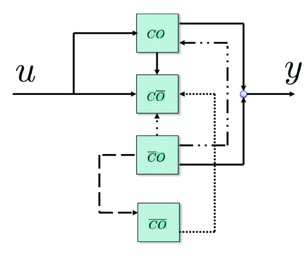
Figure 2: Kalman decomposition of a linear quantum system. Taken from Fig. 2 in [65].

The following result characterize the system parameters corresponding to the Kalman canonical form (140).

Theorem 6.2

[133, Proposition 2.1] Denote

$$\tilde{\mathbb{H}}=\mathbb{T}^{\top}\mathbb{H}\mathbb{T},\ \ \tilde{\Lambda}=\Lambda\mathbb{T},$$ (178)

where the matrices $\mathbb{H}$ and $\Lambda$ are given in Eq. (42). The real symmetric matrix $\tilde{\mathbb{H}}$ corresponding to the Kalman canonical form (140) must be of the form

$$\tilde{\mathbb{H}}=\left[\begin{array}[]{cc|c|c}0&H_{h}^{12}&0&0\\ H_{h}^{12^{\top}}&H_{h}^{22}&H_{12}&H_{13}\\ \hline\cr 0&H_{12}^{\top}&H_{co}&0\rule{0.0pt}{11.19443pt}\\ \hline\cr 0&H_{13}^{\top}&0&H_{\bar{c}\bar{o}}\rule{0.0pt}{11.19443pt}\end{array}\right],$$ (179)

and the complex matrix $\tilde{\Lambda}$ corresponding to the Kalman canonical form (140) must satisfy

$$\left[\begin{array}[]{c}\Lambda\\ \Lambda^{\#}\end{array}\right]=\left[\begin{array}[]{cc|c|c}0&\Lambda_{h}&\Lambda_{co}&0\end{array}\right],$$ (180)

where

$$\Lambda_{h}=V_{m}^{{\dagger}}C_{h},\ \ \Lambda_{co}=V_{m}^{{\dagger}}C_{co}.$$ (181)

Remark 6.1

The matrices $\Lambda_{co}$ and $\Lambda_{h}$ in Eq. (181) are respectively of the form

$$\Lambda_{co}=\left[\begin{array}[]{cc}\Lambda_{co,q}&\Lambda_{co,p}\\ \Lambda_{co,q}^{\#}&\Lambda_{co,p}^{\#}\end{array}\right],$$ (182a)

and

$$\Lambda_{h}=\left[\begin{array}[]{c}\Lambda_{h,p}\\ \Lambda_{h,p}^{\#}\end{array}\right].$$ (182b)

The Kalman canonical form (140) presented above can be used to investigate BAE measurements of quantum linear systems.

Theorem 6.3

[133, Theorem 4.1]

(i)

The quantum Kalman canonical form (140) realizes the BAE measurements of $\boldsymbol{q}_{\mathrm{out}}$ with respect to $\boldsymbol{p}_{\mathrm{in}}$; i.e., $\Xi_{\boldsymbol{p}_{\mathrm{in}}\rightarrow\boldsymbol{q}_{\mathrm{out}}}(s)\equiv 0$ if and only if

$$\left[\begin{array}[]{cc}\mathrm{Re}\left(\Lambda_{co,q}\right)&\mathrm{Re}\left(\Lambda_{co,p}\right)\end{array}\right](sI-\mathbb{J}_{n_{1}}H_{co})^{-1}\left[\begin{array}[]{c}\mathrm{Re}(\Lambda_{co,p}^{\top})\vspace{3pt}\\ -\mathrm{Re}(\Lambda_{co,q}^{\top})\end{array}\right]\equiv 0;$$ (186)

(ii)

The quantum Kalman canonical form (140) realizes the BAE measurements of $\boldsymbol{p}_{\mathrm{out}}$ with respect to $\boldsymbol{q}_{\mathrm{in}}$; i.e., $\Xi_{\boldsymbol{q}_{\mathrm{in}}\rightarrow\boldsymbol{p}_{\mathrm{out}}}(s)\equiv 0$ if and only if

$$\left[\begin{array}[]{cc}\mathrm{Im}\left(\Lambda_{co,q}\right)&\mathrm{Im}\left(\Lambda_{co,p}\right)\end{array}\right](sI-\mathbb{J}_{n_{1}}H_{co})^{-1}\left[\begin{array}[]{c}\mathrm{Im}(\Lambda_{co,p}^{\top})\vspace{3pt}\\ -\mathrm{Im}(\Lambda_{co,q}^{\top})\end{array}\right]\equiv 0.$$ (190)

6.2 An example

An opto-mechanical system has recently been physically realized in [31]. In this subsection, we analyze this system by means of the quantum Kalman canonical form presented in the previous subsection. An excellent introduction to quantum opto-mechanical systems can be found in [26].

In [31, Fig. 1(A)], an effective positive-mass oscillator and effective negative-mass oscillator coupled to a cavity are constructed to generate a quantum mechanics-free subsystem (QMFS). To be specific, the linearized Hamiltonian is [31, Eq. (S3)]

$$\mathbf{H}= \;\omega(\boldsymbol{a}_{1}^{\ast}\boldsymbol{a}_{1}-\boldsymbol{a}_{2}^{\ast}\boldsymbol{a}_{2})+g_{1}[(\alpha_{1-}\boldsymbol{a}_{1}+\alpha_{1+}\boldsymbol{a}_{1}^{\ast})\boldsymbol{a}_{3}^{\ast}+(\alpha_{1-}^{\ast}\boldsymbol{a}_{1}^{\ast}+\alpha_{1+}^{\ast}\boldsymbol{a}_{1})\boldsymbol{a}_{3}]$$ (191)

$$+\ \ g_{2}[(\alpha_{2-}\boldsymbol{a}_{2}+\alpha_{2+}\boldsymbol{a}_{2}^{\ast})\boldsymbol{a}_{3}^{\ast}+(\alpha_{2-}^{\ast}\boldsymbol{a}_{2}^{\ast}+\alpha_{2+}^{\ast}\boldsymbol{a}_{2})\boldsymbol{a}_{3}],$$

where the reduced Planck constant is omitted and $\omega$ is the detuning frequency. $\boldsymbol{a}_{j}$, $\boldsymbol{a}_{j}^{\ast}$, ($j=1,2$) denote the annihilation and creation operators for the mechanical oscillators, and their corresponding coupling strengths (to the cavity) are $G_{j\pm}=g_{j}\alpha_{j\pm}$. The cavity is characterized by the damping rate $\kappa$ and described by the annihilation and creation operators $\boldsymbol{a}_{3}$, $\boldsymbol{a}_{3}^{\ast}$. Choose equal effective couplings $|G_{j\pm}|\equiv G$ and let $G_{j\pm}=Ge^{-\imath\theta_{j\pm}}$, where $\theta_{j\pm}\in\mathbb{C}$, $j=1,2$. Then the interaction Hamiltonian (191) can be re-written as the following quadrature form [31, Eq. (S4)]

$$\mathbf{H}_{\mathrm{int}}= \;\frac{G}{2}\boldsymbol{a}_{3}[A_{-}\boldsymbol{q}_{-}+A_{+}\boldsymbol{q}_{+}+B_{-}\boldsymbol{p}_{-}+B_{+}\boldsymbol{p}_{+}]$$ (192)

$$+\ \ \frac{G}{2}\boldsymbol{a}_{3}^{\dagger}[A_{-}^{\ast}\boldsymbol{q}_{-}+A_{+}^{\ast}\boldsymbol{q}_{+}+B_{-}^{\ast}\boldsymbol{p}_{-}+B_{+}^{\ast}\boldsymbol{p}_{+}],$$

where

$$\boldsymbol{q}_{j} =\;\frac{\boldsymbol{a}_{j}^{\ast}+\boldsymbol{a}_{j}}{\sqrt{2}},~{}~{}~{}~{}\boldsymbol{p}_{j}=\frac{\imath(\boldsymbol{a}_{j}^{\ast}-\boldsymbol{a}_{j})}{\sqrt{2}},~{}~{}j=1,2,$$ (193)

$$\boldsymbol{q}_{\pm} =\frac{\boldsymbol{q}_{1}\pm\boldsymbol{q}_{2}}{\sqrt{2}},~{}~{}~{}~{}\boldsymbol{p}_{\pm}=\frac{\boldsymbol{p}_{1}\pm\boldsymbol{p}_{2}}{\sqrt{2}},$$

and

$$A_{-} =e^{-\imath\theta_{1-}}+e^{-\imath\theta_{1+}}-e^{-\imath\theta_{2-}}-e^{-\imath\theta_{2+}},$$ (194)

$$A_{+} =e^{-\imath\theta_{1-}}+e^{-\imath\theta_{1+}}+e^{-\imath\theta_{2-}}+e^{-\imath\theta_{2+}},$$

$$B_{-} =\imath[-e^{-\imath\theta_{1-}}+e^{-\imath\theta_{1+}}+e^{-\imath\theta_{2-}}-e^{-\imath\theta_{2+}}],$$

$$B_{+} =\imath[-e^{-\imath\theta_{1-}}+e^{-\imath\theta_{1+}}-e^{-\imath\theta_{2-}}+e^{-\imath\theta_{2+}}],$$

which are [31, Eq. (S5)].

Let $\theta_{1-}=\theta_{2+}=0$ and $\theta_{1+}=\theta_{2-}=\phi$. Eq. (192) becomes, [31, Eq. (S6)]

$$\mathbf{H}_{\mathrm{int}}=2G(e^{-\imath\phi/2}\boldsymbol{a}_{3}+e^{\imath\phi/2}\boldsymbol{a}_{3}^{\ast})\left(\boldsymbol{q}_{+}\cos\frac{\phi}{2}+\boldsymbol{p}_{-}\sin\frac{\phi}{2}\right).$$ (195)

Moreover, by omitting the dissipation term and choosing $\phi=0$, Eq. (195) becomes

$$\mathbf{H}_{\mathrm{int}}=2\sqrt{2}G\boldsymbol{q}_{c}\boldsymbol{q}_{+},$$ (196)

where $\boldsymbol{q}_{c}=\frac{\boldsymbol{a}_{3}^{\ast}+\boldsymbol{a}_{3}}{\sqrt{2}}$.

Remark 6.2

When $\theta_{1-}=\theta_{2+}=\theta_{1+}=\theta_{2-}=0$, all coupling strengths $G_{j\pm}=G$ are equal. This setting is used below.

Assume that the coupling strengths are equal and by the framework presented in Section 2, the system Hamiltonian (191) can be written as

$$\Omega=\Delta(\Omega_{-},\Omega_{+}),$$ (197)

where

$$\Omega_{-}=\left[\begin{array}[]{@{}ccc@{}}\omega&0&G\\ 0&-\omega&G\\ G&G&0\end{array}\right],~{}~{}~{}~{}\Omega_{+}=\left[\begin{array}[]{@{}ccc@{}}0&0&G\\ 0&0&G\\ G&G&0\end{array}\right].$$ (198)

As the optical coupling is $\boldsymbol{L}=\sqrt{\kappa}\boldsymbol{a}_{3}$ what describes energy dissipation from the cavity, we have

$$\mathcal{C}=\Delta(C_{-},C_{+}),$$ (199)

where $C_{-}=\left[\begin{array}[]{@{}ccc@{}}0&0&\sqrt{\kappa}\end{array}\right]$, $C_{+}=0$. By Eq. (18), the system matrices can be calculated as

$$\mathcal{B} =-\mathcal{C}^{\flat}=-\left[\begin{array}[]{@{}cccccc@{}}0&0&\sqrt{\kappa}&0&0&0\\ 0&0&0&0&0&\sqrt{\kappa}\end{array}\right]^{\top},$$ (200)

$$\mathcal{A} =-\imath J_{3}\Omega-\frac{1}{2}\mathcal{C}^{\flat}\mathcal{C}=\left[\begin{array}[]{@{}cccccc@{}}-\imath\omega&0&-\imath G&0&0&-\imath G\\ 0&\imath\omega&-\imath G&0&0&-\imath G\\ -\imath G&-\imath G&-\frac{\kappa}{2}&-\imath G&-\imath G&0\\ 0&0&\imath G&\imath\omega&0&\imath G\\ 0&0&\imath G&0&-\imath\omega&\imath G\\ \imath G&\imath G&0&\imath G&\imath G&-\frac{\kappa}{2}\end{array}\right].$$

As a result, the opto-mechanical system composed of two oscillators and a cavity can be described by

$$\dot{\breve{\boldsymbol{a}}} =\mathcal{A}\breve{\boldsymbol{a}}+\mathcal{B}\breve{\boldsymbol{b}}_{\rm in},$$ (201)

$$\breve{\boldsymbol{b}}_{\mathrm{out}} =\mathcal{C}\breve{\boldsymbol{a}}+\breve{\boldsymbol{b}}_{\rm in},$$

where $\boldsymbol{a}=\left[\begin{array}[]{@{}ccc@{}}\boldsymbol{a}_{1}&\boldsymbol{a}_{2}&\boldsymbol{a}_{3}\end{array}\right]^{\top}$. The auxiliary matrix $O_{s}$ defined in the proof of [65, Theorem 3.1], originally in [56, Eq. 7], can be solved by

$$O_{s}=\left[\begin{array}[]{@{}c@{}}\mathcal{C}\\ \mathcal{C}(J_{3}\Omega)\\ \vdots\\ \mathcal{C}(J_{3}\Omega)^{5}\end{array}\right].$$ (202)

In what follows, $R_{co}$, $R_{\bar{c}\bar{o}}$, $R_{c\bar{o}}$, and $R_{\bar{c}o}$ represent the controllable/observable ($co$), uncontrollable/unobservable ($\bar{c}\bar{o}$), controllable/unobservable ($c\bar{o}$), and uncontrollable/observable ($\bar{c}o$) subspaces of system (201), respectively. By [65, Lemma 4.2], these four subspaces can be calculated as

$$R_{co}=\mathrm{span}\left\{\left[\begin{array}[]{@{}c@{}}0\\ 0\\ 1\\ 0\\ 0\\ 0\end{array}\right],\left[\begin{array}[]{@{}c@{}}0\\ 0\\ 0\\ 0\\ 0\\ 1\end{array}\right]\right\},~{}~{}R_{\bar{c}\bar{o}}=\emptyset,$$ (203)

$$R_{c\bar{o}}=\mathrm{span}\left\{\left[\begin{array}[]{@{}c@{}}0\\ -1\\ 0\\ 1\\ 0\\ 0\end{array}\right],\left[\begin{array}[]{@{}c@{}}-1\\ 0\\ 0\\ 0\\ 1\\ 0\end{array}\right]\right\},~{}~{}R_{\bar{c}o}=\mathrm{span}\left\{\left[\begin{array}[]{@{}c@{}}0\\ 1\\ 0\\ 1\\ 0\\ 0\end{array}\right],\left[\begin{array}[]{@{}c@{}}1\\ 0\\ 0\\ 0\\ 1\\ 0\end{array}\right]\right\}.$$

Then by [65, Lemma 4.3] and [65, Lemma 4.7], the special orthonormal bases $T_{co}$, $T_{\bar{c}\bar{o}}$, $T_{c\bar{o}}$, and $T_{\bar{c}o}$ can be constructed. From [65, Eq. (47)], the blockwise Bogoliubov transformation matrix can be calculated as

$$T=\left[\begin{array}[]{@{}cccccc@{}}\frac{1}{\sqrt{2}}&\frac{1}{\sqrt{2}}&0&0&0&0\\ -\frac{1}{\sqrt{2}}&\frac{1}{\sqrt{2}}&0&0&0&0\\ 0&0&0&0&1&0\\ 0&0&\frac{1}{\sqrt{2}}&\frac{1}{\sqrt{2}}&0&0\\ 0&0&-\frac{1}{\sqrt{2}}&\frac{1}{\sqrt{2}}&0&0\\ 0&0&0&0&0&1\end{array}\right].$$ (204)

By [65, Theorem 4.2], we have the transformed system matrices

$$\bar{\mathcal{A}}=T^{\dagger}\mathcal{A}T,~{}~{}\bar{\mathcal{B}}=T^{\dagger}\mathcal{B},~{}~{}\bar{\mathcal{C}}=\mathcal{C}T.$$ (205)

Recall the dimensions of the four subspaces introduced in [65, Remark 4.2], we have $n_{1}=1$, $n_{2}=0$, $n_{3}=2$, and $n_{1}+n_{2}+n_{3}=n=3$ in this example. By [65, Lemma 4.8],

$$\tilde{V}_{n}=\mathrm{diag}\left\{\tilde{V}_{n_{3}},V_{n_{1}}\right\},$$ (206)

where $\tilde{V}_{n_{3}}=\Pi V_{n_{3}}$, $\Pi=\left[\begin{array}[]{@{}cccc@{}}1&0&0&0\\ 0&0&0&-1\\ 0&0&1&0\\ 0&1&0&0\end{array}\right]$, and

$$\bar{A} =\tilde{V}_{n}\bar{\mathcal{A}}\tilde{V}_{n}^{\dagger}=\left[\begin{array}[]{@{}cccccc@{}}0&-\omega&0&0&0&0\\ \omega&0&0&0&2\sqrt{2}G&0\\ 0&0&0&-\omega&0&0\\ 0&0&\omega&0&0&0\\ 0&0&0&0&-\frac{\kappa}{2}&0\\ 0&0&0&-2\sqrt{2}G&0&-\frac{\kappa}{2}\end{array}\right],$$ (207)

$$\bar{B} =\tilde{V}_{n}\bar{\mathcal{B}}V_{1}^{\dagger}=-\left[\begin{array}[]{@{}cccccc@{}}0&0&0&0&\sqrt{\kappa}&0\\ 0&0&0&0&0&\sqrt{\kappa}\end{array}\right]^{\top},$$

$$\bar{C} =V_{1}\bar{\mathcal{C}}\tilde{V}_{n}^{\dagger}=-\bar{B}^{\top}.$$

By [65, Lemma 4.9], the real, orthogonal, and blockwise symplectic matrix $\mathbb{T}\triangleq V_{n}T\tilde{V}_{n}^{\dagger}$. From [65, Theorem 4.4], the transformed system operators

$$\mathbb{T}^{\top}V_{n}\breve{\boldsymbol{a}}=\left[\begin{array}[]{@{}c@{}}\boldsymbol{q}_{-}\\ -\boldsymbol{p}_{+}\\ \boldsymbol{p}_{-}\\ \boldsymbol{q}_{+}\\ \hline\cr\boldsymbol{q}_{c}\\ \boldsymbol{p}_{c}\end{array}\right]\equiv\left[\begin{array}[]{@{}c@{}}\boldsymbol{q}_{h}\\ \boldsymbol{p}_{h}\\ \hline\cr\boldsymbol{x}_{co}\end{array}\right],$$ (208)

where $\boldsymbol{p}_{c}=\frac{\imath(\boldsymbol{a}_{3}^{\ast}-\boldsymbol{a}_{3})}{\sqrt{2}}$. By [65, Theorem 4.4], the Kalman decomposition for the opto-mechanical system (201) in the real quadrature operator representation can be expressed as

$$\dot{\boldsymbol{q}}_{h} =\left[\begin{array}[]{@{}cc@{}}0&-\omega\\ \omega&0\end{array}\right]\boldsymbol{q}_{h}+\left[\begin{array}[]{@{}cc@{}}0&0\\ 2\sqrt{2}G&0\end{array}\right]\boldsymbol{x}_{co},$$ (209)

$$\dot{\boldsymbol{p}}_{h} =\left[\begin{array}[]{@{}cc@{}}0&-\omega\\ \omega&0\end{array}\right]\boldsymbol{p}_{h},$$

$$\dot{\boldsymbol{x}}_{co} =-\frac{\kappa}{2}\boldsymbol{x}_{co}-\left[\begin{array}[]{@{}cc@{}}0&0\\ 0&2\sqrt{2}G\end{array}\right]\boldsymbol{p}_{h}-\sqrt{\kappa}\left[\begin{array}[]{@{}c@{}}\boldsymbol{q}_{\mathrm{in}}\\ \boldsymbol{p}_{\mathrm{in}}\end{array}\right],$$

$$\left[\begin{array}[]{@{}c@{}}\boldsymbol{q}_{\mathrm{out}}\\ \boldsymbol{p}_{\mathrm{out}}\end{array}\right] =\sqrt{\kappa}\boldsymbol{x}_{co}+\left[\begin{array}[]{@{}c@{}}\boldsymbol{q}_{\mathrm{in}}\\ \boldsymbol{p}_{\mathrm{in}}\end{array}\right].$$

Consequently, by omitting the dissipation term ($\kappa=0$), we have

$$\dot{\boldsymbol{q}}_{-} =\omega\boldsymbol{p}_{+},$$ (210)

$$\dot{\boldsymbol{p}}_{+} =-\omega\boldsymbol{q}_{-}-2\sqrt{2}G\boldsymbol{q}_{c},$$

$$\dot{\boldsymbol{p}}_{-} =-\omega\boldsymbol{q}_{+},$$

$$\dot{\boldsymbol{q}}_{+} =\omega\boldsymbol{p}_{-},$$

$$\dot{\boldsymbol{q}}_{c} =0,$$

$$\dot{\boldsymbol{p}}_{c} =-2\sqrt{2}G\boldsymbol{q}_{+},$$

where $\left\{\boldsymbol{q}_{+},~{}\boldsymbol{p}_{-}\right\}$ forms an isolated QMFS, and Eq. (210) is consistent with [31, Eq. (S10)].

Moreover, by Eq. (209) it can be verified that the opto-mechanical system realizes a BAE measurement of $\boldsymbol{q}_{\mathrm{out}}$ with respect to $\boldsymbol{p}_{\mathrm{in}}$, and a BAE measurement of $\boldsymbol{p}_{\mathrm{out}}$ with respect to $\boldsymbol{q}_{\mathrm{in}}$.

7 Response to single-photon states

7.1 Continuous-mode single-photon states

In this subsection, we introduce continuous-mode single-photon states of a free traveling light field.

We look at the single-channel ($m=1$) case first. Denote $\ket{1_{t}}=\mathbf{b}_{\rm in}^{\ast}(t)\ket{\Phi_{0}}$, i.e., a photon is generated at the time instant $t$ by the creation operator $\mathbf{b}_{\rm in}^{\ast}(t)$ from the vacuum field $\ket{\Phi_{0}}$. By Eq. (8) we get $\braket{1_{t}}{1_{\tau}}=\delta(t-\tau)$; in other words, the entries in $\{\ket{1_{t}}:t\in\mathbb{R}\}$ are orthogonal. Actually, $\{\ket{1_{t}}:t\in\mathbb{R}\}$ form a complete basis of continuous-mode single-photon states of a free propagating light field, in the sense that a continuous-mode single-photon state $\ket{1_{\xi}}$ of the temporal pulse shape $\xi\in L_{2}(\mathbb{R},\mathbb{C})$ can be expressed as

$$\ket{1_{\xi}}\equiv\mathbf{B}_{\rm in}^{\ast}(\xi)\ket{\Phi_{0}}\triangleq\int_{-\infty}^{\infty}\xi(t)\ket{1_{t}}dt.$$ (211)

(Here, it is assumed that the $L_{2}$ norm $\|\xi\|\triangleq\sqrt{\int_{-\infty}^{\infty}|\xi(t)|^{2}}dt=1$. Then $\braket{1_{\xi}}{1_{\xi}}=1$.) The physical interpretation of the single-photon state $\ket{1_{\xi}}$ is that the probability of detecting the photon in the time bin $[t,t+dt)$ is $|\xi(t)|^{2}dt$. In the frequency domain, we denote $\ket{1_{\omega}}\triangleq\mathbf{b}_{\rm in}^{\ast}[i\omega]\ket{0}$. Hence, in the frequency domain (211) becomes

$$\ket{1_{\xi}}=\int_{-\infty}^{\infty}\xi[i\omega]\ket{1_{\omega}}d\omega.$$ (212)

Remark 7.1

Notice

$$\langle 1_{\xi}|d\mathbf{B}_{\rm in}^{\ast}(t)d\mathbf{B}_{\rm in}(t)|1_{\xi}\rangle$$ (213)

$$= \int_{-\infty}^{\infty}\int_{-\infty}^{\infty}drd\tau\xi(r)^{\ast}\xi(\tau)\int_{t}^{t+dt}\int_{t}^{t+dt}dt_{1}dt_{2}\langle\Phi_{0}|\mathbf{b}_{\rm in}(r)\mathbf{b}_{\rm in}^{\ast}(t_{1})\mathbf{b}_{\rm in}(t_{2})\mathbf{b}_{\rm in}^{\ast}(\tau)\Phi_{0}\rangle$$

$$= \int_{t}^{t+dt}\int_{t}^{t+dt}dt_{1}dt_{2}\int_{-\infty}^{\infty}\int_{-\infty}^{\infty}drd\tau\xi(r)^{\ast}\xi(\tau)\delta(t_{1}-r)\delta(t_{2}-\tau)$$

$$= \int_{t}^{t+dt}\xi^{\ast}(t_{1})dt_{1}\int_{t}^{t+dt}\xi(t_{2})dt_{2}.$$

Thus, for most functions $\xi\in L_{2}(\mathbb{R},\mathbb{C})$,

$$\langle 1_{\xi}|d\mathbf{B}_{\rm in}^{\ast}(t)d\mathbf{B}_{\rm in}(t)|1_{\xi}\rangle=({\cal O}(dt))^{2}.$$ (214)

In Itô stochastic calculus, $\langle 1_{\xi}|d\mathbf{B}_{\rm in}^{\ast}(t)d\mathbf{B}_{\rm in}(t)|1_{\xi}\rangle=0$. This shows that the field with a continuous-mode single-photon state $\ket{1_{\xi}}$ is a canonical field.

In this tutorial, we investigate single-photon states from a control-theoretic perspective. For physical implementation of single photon generation, detection and storing, please refer to the physics literature [135, 136, 137, 138, 139, 140, 141, 142, 143, 144, 145, 146, 147, 148, 149, 150, 151, 152, 153, 154, 155, 156, 157, 158, 159] and references therein. A concise discussion can be found in [63, Section 3.1].

7.2 Response of quantum linear systems to continuous-mode single-photon states

Let the linear quantum system $G$ be initialized in the coherent state $\ket{\alpha}$ (defined in Section 4) and the input field be initialized in the vacuum state $\ket{\Phi_{0}}$. Then the initial joint system-field state is $\rho_{0g}\triangleq\ket{\alpha}\bra{\alpha}\otimes\ket{\Phi_{0}}\bra{\Phi_{0}}$ in the form of a density matrix. Denote

$$\rho_{\infty g}=\lim_{t\rightarrow\infty,t_{0}\rightarrow-\infty}U\left(t,t_{0}\right)\rho_{0g}U\left(t,t_{0}\right)^{\ast}.$$ (215)

Here, $t_{0}\to-\infty$ indicates that the interaction starts in the remote past and $t\to\infty$ means that we are interested in the dynamics in the far future. In other words, we look at the steady-state dynamics. Define

$$\rho_{{\rm field},g}\triangleq\langle\alpha|\rho_{\infty g}|\alpha\rangle.$$ (216)

In other words, the system is traced off and we focus on the steady state of the output field.

Let the $k$th input channel be in a single photon state $|1_{\mu_{k}}\rangle$, $k=1,\ldots,m$. Thus, the state of the $m$-channel input is given by the tensor product

$$|\Psi_{\mu}\rangle=|1_{\mu_{1}}\rangle\otimes\cdots\otimes|1_{\mu_{m}}\rangle.$$ (217)

Denote $\mu=[\mu_{1}\ \ \cdots\ \ \mu_{m}]^{\top}$.

Theorem 7.1

Assume that the passive linear quantum system (32) is Hurwitz stable, initialized in the vacuum state $\ket{0}$ and driven by an $m$-photon input state $|\Psi_{\mu}\rangle$ in Eq. (217). Then the steady-state output state is another $m$-photon $|\Psi_{\nu}\rangle$ whose pulse $\nu=[\nu_{1}\ \ \cdots\ \ \nu_{m}]^{\top}$ is given by

$$\nu[i\omega]=\Xi_{G^{-}}[i\omega]\mu[i\omega].$$ (218)

If the linear system $G$ is not passive, or is not initialized in the vacuum state $\ket{0}$, the steady-state output field state $\rho_{\rm out}$ in general is not a single- or multi-photon state. This new type of states has been named “photon-Gaussian” states in [64]. Moreover, it has been proved in [64] that the class of photon-Gaussian states is invariant under the steady-state action of a linear quantum system. In what follows we present this result.

Definition 7.1

[64, Definition 1] A state $\rho_{\xi,R}$ is said to be a photon-Gaussian state if it belongs to the set

$$\mathcal{F}\triangleq \;\left\{\rho_{\xi,R}=\prod\limits_{k=1}^{m}\sum_{j=1}^{m}\left(\mathbf{B}_{{\rm in},j}^{\ast}(\xi_{jk}^{-})-\mathbf{B}_{{\rm in},j}(\xi_{jk}^{+})\right)\rho_{R}\left(\prod\limits_{k=1}^{m}\sum_{j=1}^{m}\left(\mathbf{B}_{{\rm in},j}^{\ast}(\xi_{jk}^{-})-\mathbf{B}_{{\rm in},j}(\xi_{jk}^{+})\right)\right)^{\ast}\right.$$ (219)

$$\ \ \ \ \left.:\mathrm{function~{}}\xi=\Delta(\xi^{-},\xi^{+})\mathrm{~{}and~{}density~{}matrix~{}}\rho_{R}\mathrm{~{}satisfy~{}}\mathrm{Tr}[\rho_{\xi,R}]=1\right\}.$$

Theorem 7.2

[64, Theorem 5] Let $\rho_{\xi_{\rm in},R_{\rm in}}\in\mathcal{F}$ be a photon-Gaussian input state. Also, assume that $G$ is Hurwitz stable and is initialized in a coherent state $\ket{\alpha}$. Then the linear quantum system $G$ produces in steady state a photon-Gaussian output state $\rho_{\xi_{\rm out},R_{\rm out}}\in\mathcal{F}$, where

$$\xi_{\rm out}[s]= \;\Xi_{G}[s]\xi_{\rm in}[s],$$ (220)

$$R_{\rm out}[i\omega]= \;\Xi_{G}[\imath\omega]R_{\rm in}[\imath\omega]\Xi_{G}[i\omega]^{\dagger}.$$

7.3 Response of quantum linear systems to continuous-mode multi-photon states

Response of quantum linear systems to multi-photon states has been studied in [160, 161], as generalization to the single-photon case. In this subsection, we present one of the main results in these papers.

Let there be $\ell_{j}$ photons in the $j$th channel. The state for this channel is

$$\ket{\Psi_{j}}=\frac{1}{\sqrt{N_{\ell_{j}}}}\int_{\ell_{j}}\Psi_{j}(t_{1},\ldots,t_{\ell_{j}})\mathbf{b}_{{\rm in},j}^{\ast}(t_{1})\cdots\mathbf{b}_{{\rm in},j}^{\ast}(t_{\ell_{j}})dt_{1}\ldots dt_{\ell_{j}}\ket{\Phi_{0}},$$ (221)

where $\Psi_{j}$ is the pulse shape and $\sqrt{N_{\ell_{j}}}$ is the normalization coefficient. Here, for any integer $r>1$, we write $\int_{r}$ for integration in the space $\mathbb{C}^{r}$. If $\ell_{j}=0$, then Eq. (221) is understood as $\ket{\Psi_{j}}=\ket{\Phi_{0}}$. Then the state for the $m$-channel input field can be defined as

$$|\Psi\rangle=\prod\limits_{j=1}^{m}|\Psi_{j}\rangle.$$ (222)

Next, we rewrite this $m$-channel multi-photon state into an alternative form; this will enable us to present the input and output states in a unified form. For $j=1,\ldots,m$, $i=1,\ldots,\ell_{j}$, and $k_{i}=1,\ldots,m$, define functions

$$\Psi_{j,k_{1},\ldots,k_{\ell_{j}}}(\tau_{1},\ldots,\tau_{\ell_{j}})\triangleq\left\{\begin{array}[]{@{}cc@{}}\Psi_{j}(\tau_{1},\ldots,\tau_{\ell_{j}}),&k_{1}=\cdots=k_{\ell_{j}}=j,\\ 0,&\mathrm{otherwise}.\end{array}\right.$$ (223)

Then we define a class of pure $m$-channel multi-photon states

$$\mathcal{F}_{1}$$ (224)

$$= \left\{|\Psi\rangle=\prod_{j=1}^{m}\frac{1}{\sqrt{N_{\ell_{j}}}}\sum_{k_{1},\ldots,k_{\ell_{j}}=1}^{m}\int_{\ell_{j}}\Psi_{j,k_{1},\ldots,k_{\ell_{j}}}(\tau_{1},\ldots,\tau_{\ell_{j}})\right.$$

$$~{}~{}~{}~{}~{}\left.\times\prod_{i=1}^{\ell_{j}}\mathbf{b}_{{\rm in},k_{i}}^{\ast}(\tau_{i})d\tau_{1}\ldots d_{\ell_{j}}\ket{\Phi_{0}}:\langle\Psi|\Psi\rangle=1\right\}.$$

Clearly, $|\Psi\rangle$ in Eq. (222) belongs to $\mathcal{F}_{1}$.

We need some operations between matrices and tensors. Let $g_{G}(t)=(g_{G}^{jk}(t))\in\mathbb{C}^{m\times m}$ be the impulse response function of the quantum linear system $G$ in Fig. 1. For each $j=1,\ldots,m$, let $\mathscr{V}_{j}(t_{1},\ldots,t_{\ell_{j}})$ be an $\ell_{j}$-way $m$-dimensional tensor function that encodes the pulse information of the $j$th input field containing $\ell_{j}$ photons. Denote the entries of $\mathscr{V}_{j}(t_{1},\ldots,t_{\ell_{j}})$ by $\mathscr{V}_{j,k_{1},\ldots,k_{\ell_{j}}}(t_{1},\ldots,t_{\ell_{j}})$. Define an $\ell_{j}$-way $m$-dimensional tensor $\mathscr{W}_{j}$ with entries given by the following multiple convolution

$$\mathscr{W}_{j,r_{1},\ldots,r_{\ell_{j}}}(t_{1},\ldots,t_{\ell_{j}})=\sum_{k_{1},\ldots,k_{\ell_{j}}=1}^{m}\int_{\ell_{j}}g_{G}^{r_{1}k_{1}}(t_{1}-\iota_{1})\times$$

$$\cdots\times g_{G}^{r_{\ell_{j}}k_{\ell_{j}}}(t_{\ell_{j}}-\iota_{\ell_{j}})\mathscr{V}_{j,k_{1},\ldots,k_{\ell_{j}}}(\iota_{1},\ldots,\iota_{\ell_{j}})d\iota_{1}\ldots d_{\ell_{j}}$$

for all $1\leq r_{1},\ldots,r_{\ell_{j}}\leq m$. In compact form we write

$$\mathscr{W}_{j}=\mathscr{V}_{j}\times_{1}g_{G}\times_{2}\cdots\times_{\ell_{j}}g_{G},\ \ \ \forall j=1,\ldots,m,$$ (225)

cf. [162],[163, Sec. 2.5],[164] and [165].

Theorem 7.3

([160, Theorem 12]) Suppose that the quantum linear system $G$ is Hurwitz stable and passive. The steady-state output state of $G$ driven by a state $|\Psi_{\rm in}\rangle\in\mathcal{F}_{1}$ is another state $|\Psi_{\rm out}\rangle\in\mathcal{F}_{1}$ with wave packet transfer

$$\Psi_{{\rm out},j}=\Psi_{{\rm in},j}\times_{1}g_{G^{-}}\times_{2}\cdots\times_{\ell_{j}}g_{G^{-}},\ \ \ \forall j=1,\ldots,m,$$

where the operation between the matrix and tensor is defined in Eq. (225).

More discussions on continuous-mode multi-photon states can be found in [160, 161]. An application to the amplification of optical Schrödinger cat states can be found in [166]. Simply speakin, the mathematial methods proposed in [160, 161] can be used to study photon-catalyzed quabtunm non-Gaussian states, which are useful resources in quantun information processing [167, 168, 169] The problem of the response of quantum nonlinear systems to multi-photon states has been studied in [170, 171, 172, 173, 174, 175, 176, 177, 178, 179, 180, 181, 182, 183, 184, 185, 186, 187, 188, 189, 190, 191, 192, 193, 194, 76, 195]. It turns out that the linear systems theory plays a key role in some of these studies.

A continuous-mode single-photon field studied in Subsection 7.1 has statistical properties. Thus, it is natural to study the filtering problem of a quantum system driven by a continuous-mode single-photon states. Continuous-mode single-photon filters were derived in [196] and [197] first, and their multi-photon version was developed in [198, 199, 200] and [201]. A review of continuous-mode single or multi-photon states is given in [63].

8 Feedback control of quantum linear systems

Feedback control of quantum systems has been covered in several books, for example, [202, 9, 203] and [5]. In particular, the monograph [9] is devoted to the feedback control of quantum linear systems. Depending on whether the underlying quantum system (plant) is measured and the measurement data is used for the feedback control of the plant, feedback control methods of quantum systems can be roughly divided into two categories: measurement feedback control and coherent feedback control. It is clear that the former makes use of measurement information, whereas in a coherent feedback network no measurement is involved and thus coherence of quantum signals is preserved. To our understanding, measurement feedback control has been studied intensively and well recorded in [5], [202], and [203]. In contrast, coherent feedback control is still a bit new to many researchers in the quantum control community, though it has advantages in many applications [204, 1, 205, 206, 207, 208, 209, 210, 211, 212, 213, 214, 215, 25, 216, 217, 218, 219, 34, 9, 8, 220, 221, 222, 223, 224, 10, 225, 50, 11, 29, 30, 226, 227, 228, 229, 230]. Thus, in this section, we describe briefly linear quantum coherent feedback networks and use a recent experiment as demonstration.

8.1 Quantum coherent feedback linear networks

For notational simplicity, in this and the next subsections, the subscript “in” for input fields is omitted.

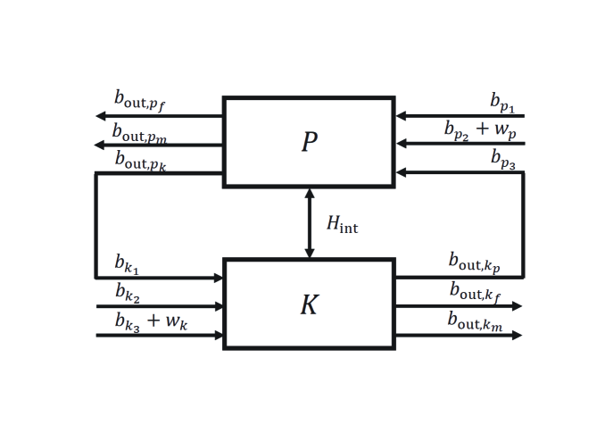
Figure 3: Coherent feedback control network.

In Fig. 3, the closed-loop system contains a quantum plant $P$ and a quantum controller $K$ to be designed. We look at the plant $P$ first, which is a quantum linear system driven by three types of input channels. To be specific, $\mathbf{b}_{p_{1}}$ describes the free input channels which may model quantum white noise such as the vacuum or thermal noise. For example, $\mathbf{b}_{p_{1}}$ can be unmodeled quantum vacuum noise on the quantum plant due to imperfection of the physical system. As discussed in Remark 2.1, $\mathbf{b}_{p_{2}}$ models the quantum vacuum fields and $w_{p}$ represents quantum or classical signals. For example, $w_{p}$ may be some undesired disturbance on the quantum plant $P$; it may also represent classical signals from a classical controller such as $u_{2}$ in [9, Figure 5.1]. The third input, which is the output $\mathbf{b}_{\mathrm{out},k_{p}}$ of the controller $K$, is denoted by $\mathbf{b}_{p_{3}}$. Correspondingly, we define three coupling operators $\mathbf{L}_{p_{1}}$, $\mathbf{L}_{p_{2}}$, $\mathbf{L}_{p_{3}}$ and three scattering matrices $S_{p_{1}}$, $S_{p_{2}}$, $S_{p_{3}}$ for the input–output channels. By means of the theory introduced in Section 2, the physical output channels are $\mathbf{b}_{\mathrm{out},p_{1}}$, $\mathbf{b}_{\mathrm{out},p_{2}}$, and $\mathbf{b}_{\mathrm{out},p_{3}}$, which in the integral form are given by

$$d\mathbf{B}_{\mathrm{out},p_{1}}(t) =\mathbf{L}_{p_{1}}(t)dt+S_{P_{1}}d\mathbf{B}_{p_{1}}(t),$$ (226)

$$d\mathbf{B}_{\mathrm{out},p_{2}}(t) =\mathbf{L}_{p_{2}}(t)dt+S_{P_{2}}(d\mathbf{B}_{p_{2}}(t)+w_{p}dt),$$

$$d\mathbf{B}_{\mathrm{out},p_{3}}(t) =\mathbf{L}_{p_{3}}(t)dt+S_{P_{3}}d\mathbf{B}_{p_{3}}(t),$$

These physical channels can be put into three categories $\mathbf{b}_{\mathrm{out},p_{f}}$, $\mathbf{b}_{\mathrm{out},p_{m}}$, and $\mathbf{b}_{\mathrm{out},p_{k}}$. Here, $\mathbf{b}_{\mathrm{out},p_{f}}$ is a set of free output channels, $\mathbf{b}_{\mathrm{out},p_{m}}$ represents a collection of output field channels which are to be measured, and $\mathbf{b}_{\mathrm{out},p_{k}}$ is a set of output channels to be sent to the controller $K$. As a result, the dynamics of the plant $P$ can be described by the following QSDEs

$$d\breve{\mathbf{a}}_{p}(t) =\;\mathcal{A}_{p}\breve{a}_{p}(t)dt+\mathcal{E}_{p}\breve{v}_{p}(t)dt+\mathcal{B}_{p_{1}}d\breve{\mathbf{B}}_{p_{1}}(t)$$ (227)

$$+\ \ \mathcal{B}_{p_{2}}(d\breve{\mathbf{B}}_{p_{2}}(t)+\breve{w}_{p}(t)dt)+\mathcal{B}_{p_{3}}d\breve{\mathbf{B}}_{p_{3}(t)},$$

$$d\breve{\mathbf{B}}_{\mathrm{out},p_{f}}(t) =\;\mathcal{C}_{p_{f}}\breve{a}_{p}(t)dt+\mathcal{D}_{p_{f1}}d\breve{\mathbf{B}}_{p_{1}}(t)$$

$$+\ \ \mathcal{D}_{p_{f2}}(d\breve{\mathbf{B}}_{p_{2}}(t)+\breve{w}_{p}(t)dt)+\mathcal{D}_{p_{f3}}d\breve{\mathbf{B}}_{p_{3}}(t),$$

$$d\breve{\mathbf{B}}_{\mathrm{out},p_{m}}(t) =\;\mathcal{C}_{p_{m}}\breve{a}_{p}(t)dt+\mathcal{D}_{p_{m1}}d\breve{\mathbf{B}}_{p_{1}}(t)$$

$$+\ \ \mathcal{D}_{p_{m2}}(d\breve{\mathbf{B}}_{p_{2}}(t)+\breve{w}_{p}(t)dt)+\mathcal{D}_{p_{m3}}d\breve{\mathbf{B}}_{p_{3}}(t),$$

$$d\breve{\mathbf{B}}_{\mathrm{out},p_{k}}(t) =\;\mathcal{C}_{p_{k}}\breve{a}_{p}(t)dt+\mathcal{D}_{p_{k1}}d\breve{\mathbf{B}}_{p_{1}}(t)$$

$$+\ \ \mathcal{D}_{p_{k2}}(d\breve{\mathbf{B}}_{p_{2}}(t)+\breve{w}_{p}(t)dt)+\mathcal{D}_{p_{k3}}d\breve{\mathbf{B}}_{p_{3}}(t).$$

Similarly, the inputs $\mathbf{b}_{k_{1}}$, $\mathbf{b}_{k_{2}}$, $\mathbf{b}_{k_{3}}$ and outputs $\mathbf{b}_{\mathrm{out},k_{p}}$, $\mathbf{b}_{\mathrm{out},k_{f}}$, $\mathbf{b}_{\mathrm{out},k_{m}}$ of the controller $K$ are labeled in Fig. 3, respectively. The QSDEs for the controller $K$ is given by

$$d\breve{\mathbf{a}}_{k}(t) =\mathcal{A}_{k}\breve{\mathbf{a}}_{k}(t)dt+\mathcal{E}_{k}\breve{v}_{k}(t)dt+\mathcal{B}_{k_{1}}d\breve{\mathbf{B}}_{k_{1}}(t)$$ (228)

$$+\ \ \mathcal{B}_{k_{2}}d\breve{\mathbf{B}}_{k_{2}}(t)+\mathcal{B}_{k_{3}}(d\breve{\mathbf{B}}_{k_{3}}(t)+\breve{w}_{k}(t)dt),$$

$$d\breve{\mathbf{B}}_{\mathrm{out},k_{p}}(t) =\mathcal{C}_{k_{p}}\breve{\mathbf{a}}_{k}(t)dt+\mathcal{D}_{k_{p2}}d\breve{\mathbf{B}}_{k_{2}}(t)+\mathcal{D}_{k_{p3}}(d\breve{\mathbf{B}}_{k_{3}}(t)+\breve{w}_{k}(t)dt),$$

$$d\breve{\mathbf{B}}_{\mathrm{out},k_{f}}(t) =\mathcal{C}_{k_{f}}\breve{\mathbf{a}}_{k}(t)dt+\mathcal{D}_{k_{f1}}d\breve{\mathbf{B}}_{k_{1}}(t)$$

$$+\ \ \mathcal{D}_{k_{f2}}d\breve{\mathbf{B}}_{k_{2}}(t)+\mathcal{D}_{k_{f3}}(d\breve{\mathbf{B}}_{k_{3}}(t)+\breve{w}_{k}(t)dt),$$

$$d\breve{\mathbf{B}}_{\mathrm{out},k_{m}}(t) =\mathcal{C}_{k_{m}}\breve{\mathbf{a}}_{k}(t)dt+\mathcal{D}_{k_{m1}}d\breve{\mathbf{B}}_{k_{1}}(t)$$

$$+\ \ \mathcal{D}_{k_{m2}}d\breve{\mathbf{B}}_{k_{2}}(t)+\mathcal{D}_{k_{m3}}(d\breve{\mathbf{B}}_{k_{3}}(t)+\breve{w}_{k}(t)dt).$$

Remark 8.1

As shown in Fig. 3, the input field $\mathbf{b}_{k_{1}}$ of the controller $K$ is the output field $\mathbf{b}_{{\rm out},p_{k}}$ of the plant $P$, and the output $\mathbf{b}_{{\rm out},k_{p}}$ of the controller $K$ is the input $\mathbf{b}_{p_{3}}$ of the plant $P$. As shown in Eq. (227) the output field $\mathbf{b}_{{\rm out},p_{k}}$ may correspond to the input field $\mathbf{b}_{p_{3}}$ which is the field $\mathbf{b}_{{\rm out},k_{p}}$. To guarantee causality, the field $\mathbf{b}_{{\rm out},k_{p}}$ must not contain the input field $\mathbf{b}_{k_{1}}=\mathbf{b}_{{\rm out},p_{k}}$. This is the reason why the evolution of $\breve{\mathbf{B}}_{\mathrm{out},k_{p}}(t)$ in Eq. (228) depends on the free traveling fields $\mathbf{b}_{k_{2}}$ and $\mathbf{b}_{k_{3}}$, but not on $\mathbf{b}_{k_{1}}$. There are other possible configurations which can guarantee causality. One example is given in Subsection 8.2 to demonstrate one such possible configuration. In this example, $\mathbf{b}_{{\rm out},p_{k}}$ corresponds to the input laser which is $\mathbf{b}_{p2}+w_{p}$. $\mathbf{b}_{{\rm out},p_{k}}$ is sent to $K$ generating the corresponding output $\mathbf{b}_{{\rm out},k_{p}}$. However, $\mathbf{b}_{{\rm out},k_{p}}$ is the input $\mathbf{b}_{p_{3}}$ of $P$ whose corresponding output is the output laser $\mathbf{b}_{{\rm out},p_{m}}$ to be measured. This fundamental assumption is also used in quantum circuits [231, Section 1.3.4].

The plant $P$ and controller $K$ can also be directly coupled via an interaction Hamiltonian $H_{\mathrm{int}}$ as labeled in Fig. 3 with the following form

$$\mathbf{H}_{\mathrm{int}}=\frac{1}{2}\left(\breve{\mathbf{a}}_{p}^{\dagger}\Xi^{\dagger}\breve{\mathbf{a}}_{k}+\breve{\mathbf{a}}_{k}^{\dagger}\Xi\breve{\mathbf{a}}_{p}\right),$$ (229)

where $\Xi=\Delta(\imath K_{-},\imath K_{+})$ for complex matrices $K_{-}$ and $K_{+}$ with suitable dimensions. It is easy to see that the commutators $[\breve{\mathbf{a}}_{p},\mathbf{H}_{\mathrm{int}}]$ and $[\breve{\mathbf{a}}_{k},\mathbf{H}_{\mathrm{int}}]$ yield

$${\mathcal{B}}_{12}=-\Delta(K_{-},K_{+})^{\flat},\ \;{\mathcal{B}}_{21}=-{\mathcal{B}}_{12}^{\flat}=\Delta(K_{-},K_{+}).$$ (230)

On the other hand, indirect coupling refers to the coupling through field channels $\breve{\mathbf{b}}_{{\rm out},P}$ and $\breve{\mathbf{b}}_{{\rm out},K}$. More discussions on direct coupling and indirect coupling can be found in, e.g., [8] and [51, 6].

The controller matrices for direct and indirect couplings are to be found to optimize performance criteria defined in terms of the set of closed-loop performance variables

$$\breve{z}(t)=[{\mathcal{C}}_{p}~{}~{}{\mathcal{C}}_{k}]\left[\begin{array}[]{@{}c@{}}\breve{\mathbf{a}}_{p}(t)\\ \breve{\mathbf{a}}_{k}(t)\end{array}\right]+{\mathcal{D}}_{z}\breve{w}(t).$$ (231)

An example of control performance variables is $z=\mathbf{a}_{p}$ for a single-mode cavity. Then $z^{\ast}z=\mathbf{a}_{p}^{\ast}\mathbf{a}_{p}=\frac{\mathbf{q}^{2}+\mathbf{p}^{2}-1}{2}$. Minimizing the mean value of $\int z^{\ast}(t)z(t)dt$ means cooling the cavity oscillator; see [232]. The form of performance variables for $H^{\infty}$ control can be found in [46, 4]. More discussions can be found in books [5, Chapter 6] and [9].

By eliminating the in-loop fields $\mathbf{b}_{{\rm out},p_{k}}$ and $\mathbf{b}_{{\rm out},k_{p}}$, the overall plant-controller quantum system, including direct and indirect couplings, can be written as

$$\left[\begin{array}[]{@{}c@{}}d\breve{\mathbf{a}}_{p}(t)\\ d\breve{\mathbf{a}}_{k}(t)\end{array}\right]= \;\left[\begin{array}[]{@{}cc@{}}\mathcal{A}_{p}&\mathcal{B}_{p_{3}}\mathcal{C}_{k_{p}}+\mathcal{B}_{12}\\ \mathcal{B}_{k_{1}}\mathcal{C}_{p_{k}}+\mathcal{B}_{21}&\mathcal{A}_{k}+\mathcal{B}_{k_{1}}\mathcal{D}_{p_{k3}}\mathcal{C}_{k_{p}}\end{array}\right]\left[\begin{array}[]{@{}c@{}}\breve{\mathbf{a}}_{p}(t)\\ \breve{\mathbf{a}}_{k}(t)\end{array}\right]dt$$ (232)

$$+\ \ \left[\begin{array}[]{@{}cc@{}}\mathcal{B}_{p_{2}}&\mathcal{B}_{p_{3}}\mathcal{D}_{k_{p3}}\\ \mathcal{B}_{k_{1}}\mathcal{D}_{p_{k2}}&\mathcal{B}_{k_{3}}+\mathcal{B}_{k_{1}}\mathcal{D}_{p_{k3}}\mathcal{D}_{k_{p3}}\end{array}\right]\left[\begin{array}[]{@{}c@{}}\breve{w}_{p}(t)\\ \breve{w}_{k}(t)\end{array}\right]dt$$

$$+\ \ \left[\begin{array}[]{@{}cc@{}}\mathcal{E}_{p}&0\\ 0&\mathcal{E}_{k}\end{array}\right]\left[\begin{array}[]{@{}c@{}}\breve{v}_{p}(t)\\ \breve{v}_{k}(t)\end{array}\right]dt+{\mathcal{G}}_{\rm cl}\left[\begin{array}[]{@{}c@{}}d\breve{\mathbf{B}}_{p_{1}}(t)\\ d\breve{\mathbf{B}}_{p_{2}}(t)\\ d\breve{\mathbf{B}}_{k_{2}}(t)\\ d\breve{\mathbf{B}}_{k_{3}}(t)\end{array}\right],$$

where

$${\mathcal{G}}_{\rm cl}=\left[\begin{array}[]{@{}cccc@{}}\mathcal{B}_{p_{1}}&\mathcal{B}_{p_{2}}&\mathcal{B}_{p_{3}}\mathcal{D}_{k_{p2}}&\mathcal{B}_{p_{3}}\mathcal{D}_{k_{p3}}\\ \mathcal{B}_{k_{1}}\mathcal{D}_{p_{k1}}&\mathcal{B}_{k_{1}}\mathcal{D}_{p_{k2}}&\mathcal{B}_{k_{2}}+\mathcal{B}_{k_{1}}\mathcal{D}_{p_{k3}}\mathcal{D}_{k_{p2}}&\mathcal{B}_{k_{3}}+\mathcal{B}_{k_{1}}\mathcal{D}_{p_{k3}}\mathcal{D}_{k_{p3}}\end{array}\right].$$ (233)

Because standard matrix algorithms commonly used in $H^{\infty}$ synthesis and LQG synthesis are for real-valued matrices, in what follows we resort to quadrature representation. Let $\mathbf{x}_{p}$, $\mathbf{x}_{k}$, $\tilde{w}_{p}$, $\tilde{w}_{k}$, $u_{p}$, $u_{k}$, ${\mathcal{U}}_{p_{1}}$, ${\mathcal{U}}_{p_{2}}$, ${\mathcal{U}}_{k_{2}}$, ${\mathcal{U}}_{k_{3}}$ be the quadrature counterparts of $\breve{\mathbf{a}}_{p}$, $\breve{\mathbf{a}}_{k}$, $\breve{w}_{p}$, $\breve{w}_{k}$, $\breve{v}_{p}$, $\breve{v}_{k}$, $\breve{\mathbf{B}}_{p_{1}}$, $\breve{\mathbf{B}}_{p_{2}}$, $\breve{\mathbf{b}}_{k_{2}}$, $\breve{\mathbf{B}}_{k_{3}}$, respectively. Then the closed-loop quantum system in the quadrature representation is given by

$$\left[\begin{array}[]{@{}c@{}}d\mathbf{x}_{p}(t)\\ d\mathbf{x}_{k}(t)\end{array}\right]= \;\mathbb{A}_{\rm cl}\left[\begin{array}[]{@{}c@{}}\mathbf{x}_{p}(t)\\ \mathbf{x}_{k}(t)\end{array}\right]dt+\mathbb{B}_{\rm cl}\left[\begin{array}[]{@{}c@{}}\tilde{w}_{p}(t)\\ \tilde{w}_{k}(t)\end{array}\right]dt$$ (234)

$$\;+\mathbb{E}_{\rm cl}\left[\begin{array}[]{@{}c@{}}u_{p}(t)\\ u_{k}(t)\end{array}\right]dt+\mathbb{G}_{\rm cl}\left[\begin{array}[]{@{}c@{}}d\mathcal{U}_{p_{1}}(t)\\ d\mathcal{U}_{p_{2}}(t)\\ d\mathcal{U}_{k_{2}}(t)\\ d\mathcal{U}_{k_{3}}(t)\end{array}\right],$$

$$\tilde{z}(t)= \;\mathbb{C}_{\rm cl}\left[\begin{array}[]{@{}c@{}}\mathbf{x}_{p}(t)\\ \mathbf{x}_{k}(t)\end{array}\right]+\mathbb{D}_{\rm cl}\tilde{w}(t),$$

where

$$\mathbb{A}_{\rm cl}= \;\left[\begin{array}[]{@{}cc@{}}\mathbb{A}_{p}&\mathbb{B}_{p_{3}}\mathbb{C}_{k_{p}}+\mathbb{B}_{12}\\ \mathbb{B}_{k_{1}}\mathbb{C}_{p_{k}}+\mathbb{B}_{21}&\mathbb{A}_{k}+\mathbb{B}_{k_{1}}\mathbb{D}_{p_{k3}}\mathbb{C}_{k_{p}}\end{array}\right],$$ (235)

$$\mathbb{B}_{\rm cl}= \;\left[\begin{array}[]{@{}cc@{}}\mathbb{B}_{p_{2}}&\mathbb{B}_{p_{3}}\mathbb{D}_{k_{p3}}\\ \mathbb{B}_{k_{1}}\mathbb{D}_{p_{k2}}&\mathbb{B}_{k_{3}}+\mathbb{B}_{k_{1}}\mathbb{D}_{p_{k3}}\mathbb{D}_{k_{p3}}\end{array}\right],\ \ \mathbb{E}_{\rm cl}=\left[\begin{array}[]{@{}cc@{}}\mathbb{E}_{p}&0\\ 0&\mathbb{E}_{k}\end{array}\right]$$

$$\mathbb{G}_{\rm cl}= \;\left[\begin{array}[]{@{}cccc@{}}\mathbb{B}_{p_{1}}&\mathbb{B}_{p_{2}}&\mathbb{B}_{p_{3}}\mathbb{D}_{k_{p2}}&\mathbb{B}_{p_{3}}\mathbb{D}_{k_{p3}}\\ \mathbb{B}_{k_{1}}\mathbb{D}_{p_{k1}}&\mathbb{B}_{k_{1}}\mathbb{D}_{p_{k2}}&\mathbb{B}_{k_{2}}+\mathbb{B}_{k_{1}}\mathbb{D}_{p_{k3}}\mathbb{D}_{k_{p2}}&\mathbb{B}_{k_{3}}+\mathbb{B}_{k_{1}}\mathbb{D}_{p_{k3}}\mathbb{D}_{k_{p3}}\end{array}\right],$$

$$\mathbb{C}_{\rm cl}= \;\left[\begin{array}[]{@{}cc@{}}\mathbb{C}_{p}&\mathbb{C}_{k}\end{array}\right],~{}~{}\mathbb{D}_{\rm cl}=\mathbb{D}_{z}.$$

8.2 An example

In this subsection, we use one example to demonstrate the coherent feedback network in Fig. 3.

A hybrid atom-optomechanical system has recently been implemented [28, Fig. 1A], in which a laser beam is used to realize couplings between an atomic spin ensemble and a micromechanical membrane. Strong coupling between these two subsystems is successfully realized in a room-temperature environment. Interesting physical phenomena, such as normal-mode splitting, coherent energy exchange between the atomic ensemble and the micromechanical membrane, and two-mode thermal noise squeezing, are observed.

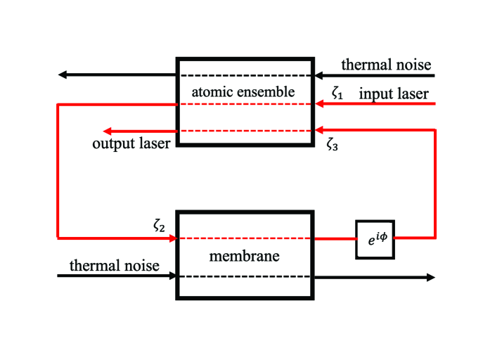
Figure 4: The system experimentally realized in [28].

This hybrid system is depicted in Fig. 4. Compared with the coherent feedback network in Fig. 3, the atomic ensemble corresponds to the plant $P$, whereas the membrane corresponds to the controller $K$. There is no direct coupling Hamiltonian $H_{\mathrm{int}}$ between the atomic ensemble and the membrane.

The atomic ensemble is modeled as a single-mode quantum mechanical oscillator which is parametrized by

$$S_{p}=I_{3},~{}\mathbf{L}_{p}=\left[\begin{array}[]{@{}c@{}}\mathbf{L}_{p1}\\ \mathbf{L}_{p2}\\ \mathbf{L}_{p3}\end{array}\right]=\left[\begin{array}[]{@{}c@{}}\sqrt{\gamma_{s}}\mathbf{q}_{s}\\ \sqrt{2\Gamma_{s}}\mathbf{q}_{s}\\ \sqrt{2\Gamma_{s}}\mathbf{q}_{s}\end{array}\right],~{}\mathbf{H}_{p}=\frac{\Omega_{s}}{2}(\mathbf{q}_{s}^{2}+\mathbf{p}_{s}^{2}),$$ (236)

where $\mathbf{q}_{s}$ and $\mathbf{p}_{s}$ are real quadrature operators of the atomic ensemble. The input laser beam is parametrized by, [8] and [43, Appendix C]

$$S_{l}=1,~{}\mathbf{L}_{l}=\sqrt{\kappa_{\mathrm{ext}}}\mathbf{a}_{l}+\alpha I,~{}\mathbf{H}_{l}=0,$$ (237)

where $\mathbf{a}_{l}$ is the annihilation operator of the laser and $\alpha\in\mathbb{C}$. Thus, $w_{p}$ in Fig. 3 is $\mathbf{L}_{l}$ in Eq. (237). By the concatenation product and the series product, the cascaded $P\vartriangleleft\mathrm{laser}$ system is

$$S_{c}=I_{3},~{}\mathbf{L}_{c}=\left[\begin{array}[]{@{}c@{}}\mathbf{L}_{c1}\\ \mathbf{L}_{c2}\\ \mathbf{L}_{c3}\end{array}\right]=\left[\begin{array}[]{@{}c@{}}\sqrt{\gamma_{s}}\mathbf{q}_{s}\\ \sqrt{2\Gamma_{s}}\mathbf{q}_{s}+\sqrt{\kappa_{\mathrm{ext}}}\mathbf{a}_{l}+\alpha I\\ \sqrt{2\Gamma_{s}}\mathbf{q}_{s}\end{array}\right],$$ (240)

$$\mathbf{H}_{c}=\frac{\Omega_{s}}{2}(\mathbf{q}_{s}^{2}+\mathbf{p}_{s}^{2})+\sqrt{\kappa_{\mathrm{ext}}\Gamma_{s}}\mathbf{q}_{s}\mathbf{p}_{l}.$$

It can be seen that the last term of $\mathbf{H}_{c}$, namely $\sqrt{\kappa_{\mathrm{ext}}\Gamma_{s}}\mathbf{q}_{s}\mathbf{p}_{l}$, describes the interaction Hamiltonian between the atomic ensemble and the light, which is consistent to the form given in [28, Eq. (S4)].

Let $\mathbf{x}_{c}$ be the real quadrature operators of the cascaded system $P\vartriangleleft\mathrm{laser}$ and $\mathbf{u}_{c}$ be the input quadrature operators. Specifically,

$$\mathbf{x}_{c}=\left[\begin{array}[]{@{}cccc@{}}\mathbf{q}_{s}&\mathbf{q}_{l}&\mathbf{p}_{s}&\mathbf{p}_{l}\end{array}\right]^{\top},$$ (241)

$$\mathbf{u}_{c}=\left[\begin{array}[]{@{}cccccc@{}}\mathbf{q}_{s}^{(\mathrm{th})}&\mathbf{q}_{s,\zeta_{1}}&\mathbf{q}_{s,\zeta_{3}}&\mathbf{p}_{s}^{(\mathrm{th})}&\mathbf{p}_{s,\zeta_{1}}&\mathbf{p}_{s,\zeta_{3}}\end{array}\right]^{\top},$$

where $(\mathbf{q}_{s}^{(\mathrm{th})},\mathbf{p}_{s}^{(\mathrm{th})})$ is input thermal noise, $(\mathbf{q}_{s,\zeta_{1}},\mathbf{p}_{s,\zeta_{1}})$ (at position $\zeta_{1}$) and $(\mathbf{q}_{s,\zeta_{3}},\mathbf{p}_{s,\zeta_{3}})$ (at position $\zeta_{3}$) denote the second and third inputs of the atomic spin ensemble, respectively. In the notation used in 3, we have system parameters

$$\left[\begin{array}[]{@{}c@{}}\mathbf{q}_{s}^{(\mathrm{th})}\\ \mathbf{p}_{s}^{(\mathrm{th})}\end{array}\right]=V_{1}\breve{b}_{p1},\ \ \left[\begin{array}[]{@{}c@{}}\mathbf{q}_{s,\zeta_{1}}\\ \mathbf{p}_{s,\zeta_{1}}\end{array}\right]=V_{1}\breve{b}_{p2},\ \ \left[\begin{array}[]{@{}c@{}}\mathbf{q}_{s,\zeta_{3}}\\ \mathbf{p}_{s,\zeta_{3}}\end{array}\right]=V_{1}\breve{b}_{p3},$$ (242)

where the unitary matrix $V_{1}$ is defined in Eq. (36). By the unitary transformations in (41), we have

$$\Lambda_{c}=\left[\begin{array}[]{@{}cccc@{}}\sqrt{\gamma_{s}}&0&0&0\\ \sqrt{2\Gamma_{s}}&\frac{\sqrt{2\kappa}}{2}&0&\frac{\sqrt{2\kappa}}{2}\imath\\ \sqrt{2\Gamma_{s}}&0&0&0\end{array}\right],$$ (246)

$$~{}\mathbb{H}_{c}=\left[\begin{array}[]{@{}cccc@{}}\Omega_{s}&0&0&\sqrt{\kappa_{\mathrm{ext}}\Gamma_{s}}\\ 0&0&0&0\\ 0&0&\Omega_{s}&0\\ \sqrt{\kappa_{\mathrm{ext}}\Gamma_{s}}&0&0&0\end{array}\right],~{}\mathbb{K}=0.$$ (251)

Consequently, by Eq. (44) the system matrices can be calculated as

$$\mathbb{D}_{c}=I_{6},~{}\mathbb{C}_{c}=\left[\begin{array}[]{@{}cccc@{}}\sqrt{2\gamma_{s}}&0&0&0\\ 2\sqrt{2\Gamma_{s}}&\sqrt{\kappa_{\mathrm{ext}}}&0&0\\ 2\sqrt{2\Gamma_{s}}&0&0&0\\ 0&0&0&0\\ 0&0&0&\sqrt{\kappa_{\mathrm{ext}}}\\ 0&0&0&0\end{array}\right],$$ (252)

$$\mathbb{B}_{c}=-\left[\begin{array}[]{@{}cccccc@{}}0&0&0&0&0&0\\ 0&\sqrt{\kappa_{\mathrm{ext}}}&0&0&0&0\\ 0&0&0&\sqrt{2\gamma_{s}}&2\sqrt{2\Gamma_{s}}&2\sqrt{2\Gamma_{s}}\\ 0&0&0&0&\sqrt{\kappa_{\mathrm{ext}}}&0\end{array}\right],$$

$$\mathbb{A}_{c}=\left[\begin{array}[]{@{}cccc@{}}0&0&\Omega_{s}&0\\ (1-\sqrt{2})\sqrt{\kappa_{\mathrm{ext}}\Gamma_{s}}&-\frac{\kappa_{\mathrm{ext}}}{2}&0&0\\ -\Omega_{s}&0&0&-(1+\sqrt{2})\sqrt{\kappa_{\mathrm{ext}}\Gamma_{s}}\\ 0&0&0&-\frac{\kappa_{\mathrm{ext}}}{2}\end{array}\right],$$

which yield the linear QSDEs that describe the dynamics of the atomic spin ensemble in the real quadrature operator representation

$$\dot{\mathbf{q}}_{s}= \Omega_{s}\mathbf{p}_{s},$$ (253)

$$\dot{\mathbf{p}}_{s}= -\Omega_{s}\mathbf{q}_{s}-(1+\sqrt{2})\sqrt{\kappa_{\mathrm{ext}}\Gamma_{s}}\mathbf{p}_{l}-2\sqrt{2\Gamma_{s}}\mathbf{p}_{s,\zeta_{1}}$$

$$-\ \ 2\sqrt{2\Gamma_{s}}\mathbf{p}_{s,\zeta_{3}}-\sqrt{2\gamma_{s}}\mathbf{p}_{s}^{(\mathrm{th})}.$$

According to Eq. (43), the output of the atomic ensemble is given by

$$\mathbb{C}_{c}\mathbf{x}_{c}+\mathbf{u}_{c}=\left[\begin{array}[]{@{}c@{}}\sqrt{2\gamma_{s}}\mathbf{q}_{s}+\mathbf{q}_{s}^{(\mathrm{th})}\\ 2\sqrt{2\Gamma_{s}}\mathbf{q}_{s}+\sqrt{\kappa_{\mathrm{ext}}}\mathbf{q}_{l}+\mathbf{q}_{s,\zeta_{1}}\\ 2\sqrt{2\Gamma_{s}}\mathbf{q}_{s}+\mathbf{q}_{s,\zeta_{3}}\\ \mathbf{p}_{s}^{(\mathrm{th})}\\ \sqrt{\kappa_{\mathrm{ext}}}\mathbf{p}_{l}+\mathbf{p}_{s,\zeta_{1}}\\ \mathbf{p}_{s,\zeta_{3}}\end{array}\right].$$ (254)

As shown in Fig. 4, the second output of the atomic spin ensemble, which is

$$\left[\begin{array}[]{@{}c@{}}2\sqrt{2\Gamma_{s}}\mathbf{q}_{s}+\sqrt{\kappa_{\mathrm{ext}}}\mathbf{q}_{l}+\mathbf{q}_{s,\zeta_{1}}\\ \sqrt{\kappa_{\mathrm{ext}}}\mathbf{p}_{l}+\mathbf{p}_{s,\zeta_{1}}\end{array}\right]=V_{1}\breve{\mathbf{b}}_{\mathrm{out},p_{k}}$$ (255)

with $\mathbf{b}_{\mathrm{out},p_{k}}$ being that in Fig. 3, is sent to the micromechanical membrane. As a result, we have

$$\left[\begin{array}[]{@{}c@{}}\mathbf{q}_{m,\zeta_{2}}(t)\\ \mathbf{p}_{m,\zeta_{2}}(t)\end{array}\right]=\left[\begin{array}[]{@{}c@{}}2\sqrt{2\Gamma_{s}}\mathbf{q}_{s}(t-\tau)+\sqrt{\kappa_{\mathrm{ext}}}\mathbf{q}_{l}(t-\tau)+\mathbf{q}_{s,\zeta_{1}}(t-\tau)\\ \sqrt{\kappa_{\mathrm{ext}}}\mathbf{p}_{l}(t-\tau)+\mathbf{p}_{s,\zeta_{1}}(t-\tau)\end{array}\right],$$ (256)

where $\tau$ denotes the time delay from the atomic spin ensemble to the micromechanical membrane in the feedback loop. Here, $\begin{smallmatrix}\left[\begin{array}[]{@{}c@{}}\mathbf{q}_{m,\zeta_{2}}(t)\\ \mathbf{p}_{m,\zeta_{2}}(t)\end{array}\right]\end{smallmatrix}=V_{1}\breve{\mathbf{b}}_{k_{1}}$ with $\breve{\mathbf{b}}_{k_{1}}$ being that in Fig. 3, is the first input to the micromechanical membrane in Fig. 4.

On the other hand, the micromechanical membrane in Fig. 4, which is a single-mode quantum harmonic oscillator too, can be parametrized by

$$S_{m}=I_{2},~{}\mathbf{L}_{m}=\left[\begin{array}[]{@{}c@{}}\mathbf{L}_{k1}\\ \mathbf{L}_{k2}\end{array}\right]=\left[\begin{array}[]{@{}c@{}}-\imath\sqrt{2\Gamma_{m}}\mathbf{q}_{m}\\ \sqrt{\gamma_{m}}\mathbf{q}_{m}\end{array}\right],~{}\mathbf{H}_{m}=\frac{\Omega_{m}}{2}(\mathbf{q}_{m}^{2}+\mathbf{p}_{m}^{2}),$$ (257)

where $\mathbf{q}_{m}$ and $\mathbf{p}_{m}$ are real quadrature operators of the micromechanical membrane. Notice that

$$\frac{\mathbf{L}_{k1}^{\ast}\mathbf{L}_{c2}-\mathbf{L}_{c2}^{\ast}\mathbf{L}_{k1}}{2\imath}=2\sqrt{\Gamma_{s}\Gamma_{m}}\mathbf{q}_{s}\mathbf{q}_{m}+\sqrt{\Gamma_{m}\kappa_{\mathrm{ext}}}\mathbf{q}_{m}\mathbf{q}_{l}+\sqrt{2\Gamma_{m}}\mathbf{q}_{m}\frac{\alpha+\alpha^{\ast}}{2}.$$ (258)

The coupling between the second output channel of the atomic ensemble and the micromechanical membrane generates several interaction Hamiltonian terms, among which the second term $\sqrt{\Gamma_{m}\kappa_{\mathrm{ext}}}\mathbf{q}_{m}\mathbf{q}_{l}$ is consistent with the form given in [28, Eq. (S14)]. As the coupling happens at $\zeta_{2}$ in Fig. 4, $\mathbf{q}_{l}$ can be written as $\mathbf{q}_{l,\zeta_{2}}$ which corresponds to $\mathbf{X}_{L}(\zeta_{m})$ in [28, Eq. (S14)].

Let $\mathbf{x}_{m}$ be the real quadrature operators of the micromechanical membrane $K$ and $\mathbf{u}_{m}$ be the input, i.e.,

$$\mathbf{x}_{m}=\left[\begin{array}[]{@{}cc@{}}\mathbf{q}_{m}&\mathbf{p}_{m}\end{array}\right]^{\top},$$ (259)

$$\mathbf{u}_{m}=\left[\begin{array}[]{@{}cccc@{}}\mathbf{q}_{m,\zeta_{2}}&\mathbf{q}_{m}^{(\mathrm{th})}&\mathbf{p}_{m,\zeta_{2}}&\mathbf{p}_{m}^{(\mathrm{th})}\end{array}\right]^{\top},$$

where $(\mathbf{q}_{m}^{(\mathrm{th})},\mathbf{p}_{m}^{(\mathrm{th})})$ is input thermal noise, and $(\mathbf{q}_{m,\zeta_{2}},\mathbf{p}_{m,\zeta_{2}})$ (at position $\zeta_{2}$) denotes the first input of the micromechanical membrane, as introduced in Eq. (256). In the notation used in Fig. 3, we have

$$\left[\begin{array}[]{@{}c@{}}\mathbf{q}_{m,\zeta_{2}}\\ \mathbf{p}_{m,\zeta_{2}}\end{array}\right]=V_{1}\breve{b}_{k1},\ \ \left[\begin{array}[]{@{}c@{}}\mathbf{q}_{m}^{(\mathrm{th})}\\ \mathbf{p}_{m}^{(\mathrm{th})}\end{array}\right]=V_{1}\breve{b}_{k2},$$ (260)

and there is no input channel associated with $b_{k3}$.

Similarly, the system matrices of the micromechanical membrane $K$ can be calculated as

$$\mathbb{D}_{m}=I_{4},~{}\mathbb{C}_{m}=\left[\begin{array}[]{@{}cc@{}}0&0\\ \sqrt{2\gamma_{m}}&0\\ -2\sqrt{\Gamma_{m}}&0\\ 0&0\end{array}\right],$$ (261)

$$\mathbb{B}_{m}=-\left[\begin{array}[]{@{}cccc@{}}0&0&0&0\\ 2\sqrt{\Gamma_{m}}&0&0&\sqrt{2\gamma_{m}}\end{array}\right],\ \ \mathbb{A}_{m}=\left[\begin{array}[]{@{}cc@{}}0&\Omega_{m}\\ -\Omega_{m}&0\end{array}\right],$$

which yields the linear QSDEs that describe the dynamics of the micromechanical membrane in the real quadrature operator representation

$$\dot{\mathbf{q}}_{m} =\Omega_{m}\mathbf{p}_{m},$$ (262)

$$\dot{\mathbf{p}}_{m} =-\Omega_{m}\mathbf{q}_{m}-2\sqrt{\Gamma_{m}}\mathbf{q}_{m,\zeta_{2}}-\sqrt{2\gamma_{m}}\mathbf{p}_{m}^{(\mathrm{th})}.$$

Substituting (256) into (262), we have

$$\dot{\mathbf{q}}_{m}(t)= \Omega_{m}\mathbf{p}_{m}(t),$$ (263)

$$\dot{\mathbf{p}}_{m}(t)= -\Omega_{m}\mathbf{q}_{m}(t)-4\sqrt{2\Gamma_{s}\Gamma_{m}}\mathbf{q}_{s}(t-\tau)-2\sqrt{\kappa_{\mathrm{ext}}\Gamma_{m}}\mathbf{q}_{l}(t-\tau)$$

$$-\ \ 2\sqrt{\Gamma_{m}}\mathbf{q}_{s,\zeta_{2}}(t)-\sqrt{2\gamma_{m}}\mathbf{p}_{m}^{(\mathrm{th})}(t).$$

Moreover, the output of the micromechanical membrane is

$$\mathbb{C}_{m}\mathbf{x}_{m}+\mathbf{u}_{m}=\left[\begin{array}[]{@{}c@{}}\mathbf{q}_{m,\zeta_{2}}\\ \sqrt{2\gamma_{m}}\mathbf{q}_{m}+\mathbf{q}_{m}^{(\mathrm{th})}\\ -2\sqrt{\Gamma_{m}}\mathbf{q}_{m}+\mathbf{p}_{m,\zeta_{2}}\\ \mathbf{p}_{m}^{(\mathrm{th})}\end{array}\right].$$ (264)

The first output of the micromechanical membrane, which is

$$\left[\begin{array}[]{@{}c@{}}\mathbf{q}_{m,\zeta_{2}}\\ -2\sqrt{\Gamma_{m}}\mathbf{q}_{m}+\mathbf{p}_{m,\zeta_{2}}\end{array}\right]=V_{1}\breve{\mathbf{b}}_{\mathrm{out},k_{p}}$$ (265)

with $\mathbf{b}_{\mathrm{out},k_{p}}$ being that in Fig. 3, is sent to the atomic spin ensemble. Noticing the phase shifter $e^{\imath\phi}$ on the way, we have

$$b_{p_{3}}(t)=e^{\imath\phi}b_{\mathrm{out},k_{p}}(t-\tau).$$ (266)

By Eqs. (264), (266) and noticing Eq. (242), we get

$$\mathbf{q}_{s,\zeta_{3}}(t) =\cos\phi\;\mathbf{q}_{m,\zeta_{2}}(t-\tau)-\sin\phi\left[-2\sqrt{\Gamma_{m}}\mathbf{q}_{m}(t-\tau)+\mathbf{p}_{m,\zeta_{2}}(t-\tau)\right],$$ (267)

$$\mathbf{p}_{s,\zeta_{3}}(t) =\cos\phi\left[-2\sqrt{\Gamma_{m}}\mathbf{q}_{m}(t-\tau)+\mathbf{p}_{m,\zeta_{2}}(t-\tau)\right]+\sin\phi\mathbf{q}_{m,\zeta_{2}}(t-\tau).$$

Substituting Eq. (256) into Eq. (267), yields

$$\mathbf{p}_{s,\zeta_{3}}(t)= -2\cos\phi\sqrt{\Gamma_{m}}\mathbf{q}_{m}(t-\tau)+2\sin\phi\sqrt{2\Gamma_{s}}\mathbf{q}_{s}(t-2\tau)$$ (268)

$$+\ \ \cos\phi\sqrt{\kappa_{\mathrm{ext}}}\mathbf{p}_{l}(t-2\tau)+\sin\phi\sqrt{\kappa_{\mathrm{ext}}}\mathbf{q}_{l}(t-2\tau)$$

$$+\ \ \cos\phi\mathbf{p}_{s,\zeta_{1}}(t-2\tau)+\sin\phi\mathbf{q}_{s,\zeta_{1}}(t-2\tau).$$

Thus, Eq. (253) can be rewritten as

$$\dot{\mathbf{q}}_{s}(t)= \Omega_{s}\mathbf{p}_{s}(t),$$ (269)

$$\dot{\mathbf{p}}_{s}(t)= -\Omega_{s}\mathbf{q}_{s}(t)-(1+\sqrt{2})\sqrt{\kappa_{\mathrm{ext}}\Gamma_{s}}\mathbf{p}_{l}(t)-2\cos\phi\sqrt{2\kappa_{\mathrm{ext}}\Gamma_{s}}\mathbf{p}_{l}(t-2\tau)$$

$$-\ \ 2\sin\phi\sqrt{2\kappa_{\mathrm{ext}}\Gamma_{s}}\mathbf{q}_{l}(t-2\tau)-8\sin\phi\Gamma_{s}\mathbf{q}_{s}(t-2\tau)$$

$$+\ \ 4\cos\phi\sqrt{2\Gamma_{s}\Gamma_{m}}\mathbf{q}_{m}(t-\tau)$$

$$-\ \ 2\sqrt{2\Gamma_{s}}\left[\mathbf{p}_{s,\zeta_{1}}(t)+\cos\phi\mathbf{p}_{s,\zeta_{3}}(t)+\sin\phi\mathbf{q}_{s,\zeta_{3}}(t)\right]-\sqrt{2\gamma_{s}}\mathbf{p}_{s}^{(\mathrm{th})}(t).$$

Despite of the terms containing laser loss $\kappa_{\mathrm{ext}}$, the dynamical equations of the micromechanical membrane (263) and the atomic spin ensemble (269) are consistent with the forms given in [28, Eqs. (S54–S58)].

Remark 8.2

In the following, we only look into the input–output channel with the laser, i.e. ignoring the thermal noise inputs. Notice that $\mathbf{L}_{p2}=\sqrt{2\Gamma_{s}}\mathbf{q}_{s}$ is the coupling between the spin and the input light, and $\mathbf{L}_{k1}=-\imath\sqrt{2\Gamma_{m}}\mathbf{q}_{m}$ is the membrane–light coupling. The coherent feedback loop can be divided into two parts. The first part is from the spin to the membrane, according to Eq. (239) whose interaction Hamiltonian is given by

$$\mathbf{H}_{\mathrm{int}}^{(1)}=\frac{1}{2\imath}(\mathbf{L}_{k1}^{\ast}\mathbf{L}_{p2}-\mathbf{L}_{p2}^{\ast}\mathbf{L}_{k1})=2\sqrt{\Gamma_{m}\Gamma_{s}}\mathbf{q}_{m}\mathbf{q}_{s},$$ (270)

and the cascaded coupling operator $\mathbf{L}^{(1)}=\mathbf{L}_{k1}+\mathbf{L}_{p2}$. The second part is from the membrane to the spin with the phase shifter $e^{\imath\phi}$ on the way, the corresponding interaction Hamiltonian is

$$\mathbf{H}_{\mathrm{int}}^{(2)}=\frac{1}{2\imath}(\mathbf{L}_{p3}^{\ast}e^{\imath\phi}\mathbf{L}^{(1)}-\mathbf{L}^{(1)\ast}e^{-\imath\phi}\mathbf{L}_{p3})=-2\sqrt{\Gamma_{m}\Gamma_{s}}\cos\phi\mathbf{q}_{s}\mathbf{q}_{m}+2\sin\phi\Gamma_{s}\mathbf{q}_{s}^{2},$$ (271)

and the cascaded coupling operator

$$\mathbf{L}^{(2)}=\mathbf{L}_{p3}+e^{\imath\phi}\mathbf{L}^{(1)}=-\imath e^{\imath\phi}\sqrt{2\Gamma_{m}}\mathbf{q}_{m}+(1+e^{\imath\phi})\sqrt{2\Gamma_{s}}\mathbf{q}_{s},$$ (272)

which is consistent with the collective jump operator $\mathbf{J}$ used in [28, Eq. (1)]. Combining Eq. (270) with Eq. (271), the interaction Hamiltonian between the atomic spin ensemble and the micromechanical membrane is

$$\mathbf{H}_{sm}=(1-\cos\phi)2\sqrt{\Gamma_{m}\Gamma_{s}}\mathbf{q}_{s}\mathbf{q}_{m}+2\sin\phi\Gamma_{s}\mathbf{q}_{s}^{2},$$ (273)

which is consistent with the effective interaction Hamiltonian $\mathbf{H}_{\rm eff}$ used in [28, Eq. (1)]. In summary, all the essential equations in [28] can be reproduced by means of the quantum linear systems and network theory introduced in this tutorial.

9 Conclusion

In this tutorial, we have given a concise introduction to linear quantum systems, for example, their mathematical models, relation between their control-theoretic properties and physical properties, Gaussian states, quantum Kalman filter, Kalman canonical form, and response to continuous-mode single-photon states. Several simple examples are designed to demonstrate some fundamental properties of linear quantum systems. Pointers to more detailed discussions are given in various places. It is hoped that this tutorial is helpful to researchers in the control community who are interested in quantum control of dynamical systems. Finally, an information-theoretic uncertainty relation has been recorded in this tutorial, which describes uncertainties of mixed quantum Gaussian states better than the Heisenberg uncertainty relation. It is an open question whether this uncertainty relation is useful for mixed quantum Gaussian state engineering.

Acknowledgement. We would like to thank Bo Qi, Liying Bao and Shuangshuang Fu for their careful reading and constructive suggestions.

References

• [1] H. M. Wiseman, G. J. Milburn, All-optical versus electro-optical quantum-limited feedback, Physical Review A 49 (5) (1994) 4110.
• [2] C. Gardiner, P. Zoller, Quantum Noise, Springer, 2004.
• [3] D. F. Walls, G. J. Milburn, Quantum Optics, Springer Science & Business Media, 2007.
• [4] H. Mabuchi, Coherent-feedback quantum control with a dynamic compensator, Physical Review A 78 (3) (2008) 032323.
• [5] H. M. Wiseman, G. J. Milburn, Quantum Measurement and Control, Cambridge University Press, 2010.
• [6] G. Zhang, M. R. James, Quantum feedback networks and control: a brief survey, Chinese Science Bulletin 57 (18) (2012) 2200–2214.
• [7] I. R. Petersen, Quantum linear systems theory, in: Proceedings of the 19th International Symposium on Mathematical Theory of Networks and Systems, Budapest, Hungary, 2010, pp. 2173–2184.
• [8] J. Combes, J. Kerckhoff, M. Sarovar, The SLH framework for modeling quantum input-output networks, Advances in Physics: X 2 (3) (2017) 784–888.
• [9] H. I. Nurdin, N. Yamamoto, Linear Dynamical Quantum Systems - Analysis, Synthesis, and Control, Springer-Verlag Berlin, 2017.
• [10] I. R. Petersen, M. R. James, V. Ugrinovskii, N. Yamamoto, A systems theory approach to the synthesis of minimum noise non-reciprocal phase-insensitive quantum amplifiers, in: 2020 59th IEEE Conference on Decision and Control (CDC), IEEE, 2020, pp. 3836–3841.
• [11] J. Bentley, H. I. Nurdin, Y. Chen, H. Miao, Direct approach to realizing quantum filters for high-precision measurements, Physical Review A 103 (1) (2021).
• [12] A. Mátyás, C. Jirauschek, F. Peretti, P. Lugli, G. Csaba, Linear circuit models for on-chip quantum electrodynamics, IEEE Transactions on Microwave Theory and Techniques 59 (1) (2010) 65–71.
• [13] D. Bozyigit, C. Lang, L. Steffen, J. Fink, C. Eichler, M. Baur, R. Bianchetti, P. J. Leek, S. Filipp, M. P. Da Silva, et al., Antibunching of microwave-frequency photons observed in correlation measurements using linear detectors, Nature Physics 7 (2) (2011) 154–158.
• [14] J. Kerckhoff, R. W. Andrews, H. Ku, W. F. Kindel, K. Cicak, R. W. Simmonds, K. Lehnert, Tunable coupling to a mechanical oscillator circuit using a coherent feedback network, Physical Review X 3 (2) (2013) 021013.
• [15] A. Blais, A. L. Grimsmo, S. Girvin, A. Wallraff, Circuit quantum electrodynamics, Reviews of Modern Physics 93 (2) (2021) 025005.
• [16] A. C. Doherty, K. Jacobs, Feedback control of quantum systems using continuous state estimation, Physical Review A 60 (4) (1999) 2700.
• [17] C. Sayrin, I. Dotsenko, X. Zhou, B. Peaudecerf, T. Rybarczyk, S. Gleyzes, P. Rouchon, M. Mirrahimi, H. Amini, M. Brune, et al., Real-time quantum feedback prepares and stabilizes photon number states, Nature 477 (7362) (2011) 73–77.
• [18] H. Amini, R. A. Somaraju, I. Dotsenko, C. Sayrin, M. Mirrahimi, P. Rouchon, Feedback stabilization of discrete-time quantum systems subject to non-demolition measurements with imperfections and delays, Automatica 49 (9) (2013) 2683–2692.
• [19] M. Tsang, C. M. Caves, Coherent quantum-noise cancellation for optomechanical sensors, Physical Review Letters 105 (12) (2010) 123601.
• [20] F. Massel, T. T. Heikkilä, J.-M. Pirkkalainen, S.-U. Cho, H. Saloniemi, P. J. Hakonen, M. A. Sillanpää, Microwave amplification with nanomechanical resonators, Nature 480 (7377) (2011) 351–354.
• [21] R. Hamerly, H. Mabuchi, Advantages of coherent feedback for cooling quantum oscillators, Physical Review Letters 109 (17) (2012) 173602.
• [22] C. Dong, V. Fiore, M. C. Kuzyk, H. Wang, Optomechanical dark mode, Science 338 (6114) (2012) 1609–1613.
• [23] F. Massel, S. U. Cho, J.-M. Pirkkalainen, P. J. Hakonen, T. T. Heikkilä, M. A. Sillanpää, Multimode circuit optomechanics near the quantum limit, Nature Communications 3 (1) (2012) 1–6.
• [24] N. Yamamoto, Decoherence-free linear quantum subsystems, IEEE Transactions on Automatic Control 59 (7) (2014) 1845–1857.
• [25] N. Yamamoto, Coherent versus measurement feedback: Linear systems theory for quantum information, Physical Review X 4 (4) (2014) 041029.
• [26] M. Aspelmeyer, T. J. Kippenberg, F. Marquardt, Cavity optomechanics, Reviews of Modern Physics 86 (4) (2014) 1391.
• [27] C. Ockeloen-Korppi, E. Damskägg, J.-M. Pirkkalainen, A. Clerk, M. Woolley, M. Sillanpää, Quantum backaction evading measurement of collective mechanical modes, Physical Review Letters 117 (14) (2016) 140401.
• [28] T. M. Karg, B. Gouraud, C. T. Ngai, G.-L. Schmid, K. Hammerer, P. Treutlein, Light-mediated strong coupling between a mechanical oscillator and atomic spins 1 meter apart, Science 369 (6500) (2020) 174–179.
• [29] S. Kotler, G. A. Peterson, E. Shojaee, F. Lecocq, K. Cicak, A. Kwiatkowski, S. Geller, S. Glancy, E. Knill, R. W. Simmonds, et al., Direct observation of deterministic macroscopic entanglement, Science 372 (6542) (2021) 622–625.
• [30] C. A. Potts, E. Varga, V. A. Bittencourt, S. V. Kusminskiy, J. P. Davis, Dynamical backaction magnomechanics, Physical Review X 11 (3) (2021) 031053.
• [31] L. M. de Lépinay, C. F. Ockeloen-Korppi, M. J. Woolley, M. A. Sillanpää, Quantum mechanics–free subsystem with mechanical oscillators, Science 372 (6542) (2021) 625–629.
• [32] J. K. Stockton, R. Van Handel, H. Mabuchi, Deterministic dicke-state preparation with continuous measurement and control, Physical Review A 70 (2) (2004) 022106.
• [33] H. I. Nurdin, M. R. James, I. R. Petersen, Coherent quantum LQG control, Automatica 45 (8) (2009) 1837–1846.
• [34] T. Astner, S. Nevlacsil, N. Peterschofsky, A. Angerer, S. Rotter, S. Putz, J. Schmiedmayer, J. Majer, Coherent coupling of remote spin ensembles via a cavity bus, Physical Review Letters 118 (14) (2017) 140502.
• [35] Q. Xu, P. Dong, M. Lipson, Breaking the delay-bandwidth limit in a photonic structure, Nature Physics 3 (6) (2007) 406–410.
• [36] Q. He, M. Reid, E. Giacobino, J. Cviklinski, P. Drummond, Dynamical oscillator-cavity model for quantum memories, Physical Review A 79 (2) (2009) 022310.
• [37] M. Hush, A. Carvalho, M. Hedges, M. James, Analysis of the operation of gradient echo memories using a quantum input–output model, New Journal of Physics 15 (8) (2013) 085020.
• [38] N. Yamamoto, M. R. James, Zero-dynamics principle for perfect quantum memory in linear networks, New Journal of Physics 16 (7) (2014) 073032.
• [39] H. Nurdin, J. Gough, Modular quantum memories using passive linear optics and coherent feedback, Quantum Information and Computation 15 (2015) 1017–1040.
• [40] I. R. Petersen, Networked quantum systems, in: Uncertainty in Complex Networked Systems, Springer, 2018, pp. 583–618.
• [41] J. E. Gough, M. R. James, H. I. Nurdin, Squeezing components in linear quantum feedback networks, Physical Review A 81 (2) (2010) 023804.
• [42] S. C. Edwards, V. P. Belavkin, Optimal quantum filtering and quantum feedback control, arXiv preprint quant-ph/0506018 (2005).
• [43] D. J. van Woerkom, P. Scarlino, J. H. Ungerer, C. Müller, J. V. Koski, A. J. Landig, C. Reichl, W. Wegscheider, T. Ihn, K. Ensslin, et al., Microwave photon-mediated interactions between semiconductor qubits, Physical Review X 8 (4) (2018) 041018.
• [44] H. Wiseman, A. Doherty, Optimal unravellings for feedback control in linear quantum systems, Physical Review Letters 94 (7) (2005) 070405.
• [45] R. L. Hudson, K. R. Parthasarathy, Quantum ito’s formula and stochastic evolutions, Communications in Mathematical Physics 93 (3) (1984) 301–323.
• [46] M. R. James, H. I. Nurdin, I. R. Petersen, ${H}^{\infty}$ control of linear quantum stochastic systems, IEEE Transactions on Automatic Control 53 (8) (2008) 1787–1803.
• [47] J. Gough, M. James, H. Nurdin, Quantum trajectories for a class of continuous matrix product input states, New Journal of Physics 16 (7) (2014) 075008.
• [48] J. E. Gough, G. Zhang, Generating nonclassical quantum input field states with modulating filters, EPJ Quantum Technology 2 (2015) 2–15.
• [49] W. Li, G. Zhang, R.-B. Wu, On the control of flying qubits, arXiv preprint arXiv:2111.00143 (2021).
• [50] R. Shimazu, N. Yamamoto, Quantum functionalities via feedback amplification, Physical Review Applied 15 (4) (2021) 044006.
• [51] G. Zhang, M. R. James, Direct and indirect couplings in coherent feedback control of linear quantum systems, IEEE Transactions on Automatic Control 56 (2011) 1535–1550.
• [52] G. Zhang, H. W. Joseph Lee, B. Huang, H. Zhang, Coherent feedback control of linear quantum optical systems via squeezing and phase shift, SIAM Journal on Control and Optimization 50 (4) (2012) 2130–2150.
• [53] H. I. Nurdin, M. R. James, A. C. Doherty, Network synthesis of linear dynamical quantum stochastic systems, SIAM Journal on Control and Optimization 48 (4) (2009) 2686–2718.
• [54] A. Maalouf, I. Petersen, Bounded real properties for a class of annihilation-operator linear quantum systems, IEEE Transactions on Automatic Control 56 (2011) 786–801.
• [55] A. Shaiju, I. Petersen, A frequency domain condition for the physical realizability of linear quantum systems, IEEE Transactions on Automatic Control 57 (2012) 2033–2044.
• [56] J. E. Gough, G. Zhang, On realization theory of quantum linear systems, Automatica 59 (2015) 139–151.
• [57] S. Wang, H. I. Nurdin, G. Zhang, M. R. James, Quantum optical realization of classical linear stochastic systems, Automatica 49 (10) (2013) 3090–3096.
• [58] S. Wang, H. I. Nurdin, G. Zhang, M. R. James, Representation and network synthesis for a class of mixed quantum–classical linear stochastic systems, Automatica 96 (2018) 84–97.
• [59] L. A. Duffaut Espinosa, Z. Miao, I. R. Petersen, V. Ugrinovskii, M. R. James, Physical realizability and preservation of commutation and anticommutation relations for n-level quantum systems, SIAM Journal on Control and Optimization 54 (2) (2016) 632–661.
• [60] M. F. Emzir, M. J. Woolley, I. R. Petersen, On physical realizability of nonlinear quantum stochastic differential equations, Automatica 95 (2018) 254–265.
• [61] B. D. Anderson, S. Vongpanitlerd, Network Analysis and Synthesis: A Modern Systems Theory Approach, Prentice Hall, Englewood Cliffs, New Jersey, 1973.
• [62] W. R. Le Page, Complex Variables and the Laplace Transform for Engineers, Courier Corporation, 1980.
• [63] G. Zhang, Control engineering of continuous-mode single-photon states: a review, Control Theory and Technology, arXiv:1902.10961v7 [quant-ph] 19 (2021).
• [64] G. Zhang, M. R. James, On the response of quantum linear systems to single photon input fields, IEEE Transactions on Automatic Control 58 (5) (2013) 1221–1235.
• [65] G. Zhang, S. Grivopoulos, I. R. Petersen, J. E. Gough, The Kalman decomposition for linear quantum systems, IEEE Transactions on Automatic Control 63 (2) (2018) 331–346.
• [66] R. E. Kalman, Mathematical description of linear dynamical systems, Journal of the Society for Industrial and Applied Mathematics, Series A: Control 1 (2) (1963) 152–192.
• [67] H. Kwakernaak, R. Sivan, Linear Optimal Control Systems, Vol. 1, Wiley-interscience New York, 1972.
• [68] H. Kimura, Chain-scattering Approach to ${H}^{\infty}$ Control, Springer Science & Business Media, 1996.
• [69] K. Zhou, J. C. Doyle, K. Glover, Robust and Optimal Control, Prentice Hall, Englewood Cliffs, New Jersey, 1996.
• [70] Y.-D. Wang, A. A. Clerk, Using interference for high fidelity quantum state transfer in optomechanics, Physical Review Letters 108 (15) (2012) 153603.
• [71] Y. Pan, D. Dong, I. Petersen, Dark modes of quantum linear systems, IEEE Transactions on Automatic Control 62 (2017) 4180–4186.
• [72] J. Huang, D.-G. Lai, C. Liu, J.-F. Huang, F. Nori, J.-Q. Liao, Multimode optomechanical cooling via general dark-mode control, arXiv preprint: 2110.14885 (2021).
• [73] S. Zhang, D. Dong, K. Liu, Dark modes in non-markovian linear quantum systems, arXiv preprint arXiv:2103.16749 (2021).
• [74] D. A. Lidar, I. L. Chuang, K. B. Whaley, Decoherence-free subspaces for quantum computation, Physical Review Letters 81 (1998) 2594–2597.
• [75] F. Ticozzi, L. Viola, Quantum markovian subsystems: invariance, attractivity, and control, IEEE Transactions on Automatic Control 53 (9) (2008) 2048–2063.
• [76] Z. Dong, G. Zhang, A.-G. Wu, R.-B. Wu, On the dynamics of the Tavis-Cummings model, arXiv preprint: 2110.14174 (2021).
• [77] K. S. Thorne, R. W. Drever, C. M. Caves, M. Zimmermann, V. D. Sandberg, Quantum nondemolition measurements of harmonic oscillators, Physical Review Letters 40 (11) (1978) 667.
• [78] V. B. Braginsky, Y. I. Vorontsov, K. S. Thorne, Quantum nondemolition measurements, Science 209 (4456) (1980) 547–557.
• [79] H. Wiseman, Using feedback to eliminate back-action in quantum measurements, Physical Review A 51 (3) (1995) 2459.
• [80] M. Tsang, C. M. Caves, Evading quantum mechanics: engineering a classical subsystem within a quantum environment, Physical Review X 2 (3) (2012) 031016.
• [81] M. Woolley, A. Clerk, Two-mode back-action-evading measurements in cavity optomechanics, Physical Review A 87 (6) (2013) 063846.
• [82] C. Møller, R. Thomas, G. Vasilakis, E. Zeuthen, M. Tsaturyan, Y.and Balabas, K. Jensen, A. Schliesser, K. Hammerer, E. Polzik, Quantum back-action-evading measurement of motion in a negative mass reference frame, Nature 547 (7662) (2017) 191–195.
• [83] I. Vladimirov, I. Petersen, Direct coupling coherent quantum observers with discounted mean square performance criteria and penalized back-action, Mathematics of Control, Signals, and Systems (2022).
• [84] M. G. Paris, F. Illuminati, A. Serafini, S. De Siena, Purity of Gaussian states: Measurement schemes and time evolution in noisy channels, Physical Review A 68 (1) (2003) 012314.
• [85] K. Parthasarathy, What is a Gaussian state?, Communications on Stochastic Analysis 4 (2) (2010) 2.
• [86] N. C. Menicucci, S. T. Flammia, P. van Loock, Graphical calculus for Gaussian pure states, Physical Review A 83 (4) (2011) 042335.
• [87] K. Koga, N. Yamamoto, Dissipation-induced pure Gaussian state, Physical Review A 85 (2) (2012) 022103.
• [88] I. Vladimirov, I. Petersen, M. James, Effects of parametric uncertainties in cascaded open quantum harmonic oscillators and robust generation of Gaussian invariant states, SIAM Journal on Control and Optimization 57 (2019) 1597–1628.
• [89] S. Ma, M. J. Woolley, I. R. Petersen, N. Yamamoto, Linear open quantum systems with passive hamiltonians and a single local dissipative process, Automatica 125 (2021) 109477.
• [90] S. Ma, M. J. Woolley, I. R. Petersen, Synthesis of linear quantum systems to generate a steady thermal state, IEEE Transactions on Automatic Control (2021).
• [91] L. Bao, B. Qi, D. Dong, Stabilizing preparation of quantum Gaussian states via continuous measurement, arXiv preprint: 2109.12748 (2021).
• [92] J. Gough, Quantum white noise and the master equation for Gaussian reference states, arXiv preprint quant-ph/0609040 (2006).
• [93] S. L. Braunstein, P. Van Loock, Quantum information with continuous variables, Reviews of Modern Physics 77 (2) (2005) 513.
• [94] N. C. Menicucci, P. Van Loock, M. Gu, C. Weedbrook, T. C. Ralph, M. A. Nielsen, Universal quantum computation with continuous-variable cluster states, Physical Review Letters 97 (11) (2006) 110501.
• [95] A. Furusawa, P. Van Loock, Quantum teleportation and entanglement: a hybrid approach to optical quantum information processing, John Wiley & Sons, 2011.
• [96] C. Weedbrook, S. Pirandola, R. García-Patrón, N. J. Cerf, T. C. Ralph, J. H. Shapiro, S. Lloyd, Gaussian quantum information, Reviews of Modern Physics 84 (2012) 621–669.
• [97] S. Ma, Pure Gaussian states in open quantum systems, Ph.D. thesis, School of Engineering and Information Technology, UNSW Canberra (2017).
• [98] S. Ma, M. J. Woolley, I. R. Petersen, N. Yamamoto, Cascade and locally dissipative realizations of linear quantum systems for pure Gaussian state covariance assignment, Automatica 90 (2018) 263–270.
• [99] S. Ma, M. J. Woolley, X. Jia, J. Zhang, Preparation of bipartite bound entangled Gaussian states in quantum optics, Physical Review A 100 (2) (2019) 022309.
• [100] S. Luo, Heisenberg uncertainty relation for mixed states, Physical Review A 72 (4) (2005) 042110.
• [101] E. P. Wigner, M. M. Yanase, Information contents of distributions, Proceedings of the National Academy of Sciences 49 (6) (1963) 910–918.
• [102] S. Fu, S. Luo, Y. Zhang, Gaussian states as minimum uncertainty states, Physics Letters A 384 (1) (2020) 126037.
• [103] P. Gibilisco, T. Isola, A characterisation of Wigner–Yanase skew information among statistically monotone metrics, Infinite Dimensional Analysis, Quantum Probability and Related Topics 4 (04) (2001) 553–557.
• [104] S. Luo, Wigner-Yanase skew information vs. quantum fisher information, Proceedings of the American Mathematical Society 132 (3) (2004) 885–890.
• [105] S. Luo, Quantum versus classical uncertainty, Theoretical and Mathematical Physics 143 (2) (2005) 681–688.
• [106] Z. Chen, Wigner-Yanase skew information as tests for quantum entanglement, Physical Review A 71 (2005) 052302.
• [107] F. Hansen, Metric adjusted skew information, Proceedings of the National Academy of Sciences 105 (29) (2008) 9909–9916.
• [108] S. Luo, S. Fu, C. H. Oh, Quantifying correlations via the Wigner-Yanase skew information, Physical Review A 85 (2012) 032117.
• [109] G. Karpat, B. Çakmak, F. F. Fanchini, Quantum coherence and uncertainty in the anisotropic XY chain, Physical Review B 90 (2014) 104431.
• [110] S. Luo, Y. Sun, Quantum coherence versus quantum uncertainty, Physical Review A 96 (2017) 022130.
• [111] Y. Sun, Y. Mao, S. Luo, From quantum coherence to quantum correlations, EPL (Europhysics Letters) 118 (6) (2017) 60007.
• [112] S. Luo, Y. Sun, Coherence and complementarity in state-channel interaction, Physical Review A 98 (2018) 012113.
• [113] S. Luo, Y. Zhang, Quantifying nonclassicality via Wigner-Yanase skew information, Physical Review A 100 (2019) 032116.
• [114] L. Bouten, R. van Handel, M. R. James, An introduction to quantum filtering, SIAM Journal on Control and Optimization 46 (6) (2007) 2199–2241.
• [115] H. J. Carmichael, Quantum trajectory theory for cascaded open systems, Phys. Rev. Lett. 70 (1993) 2273–2276.
• [116] H. Carmichael, An Open Systems Approach to Quantum Optics, Vol. 18, Springer Science & Business Media, 2009.
• [117] V. P. Belavkin, Quantum filtering of markov signals with white quantum noise, Elektronika 25 (1980) 1445–1453.
• [118] V. P. Belavkin, Nondemolition measurements, nonlinear filtering and dynamic programming of quantum stochastic processes, in: Modeling and Control of Systems, Springer, 1989, pp. 245–265.
• [119] A. C. Doherty, S. Habib, K. Jacobs, H. Mabuchi, S. M. Tan, Quantum feedback control and classical control theory, Physical Review A 62 (1) (2000) 012105.
• [120] R. van Handel, J. Stockton, H. Mabuchi, Feedback control of quantum state reduction, IEEE Transactions on Automatic Control 50 (6) (2005) 768–780.
• [121] R. van Handel, Filtering, stability, and robustness, Ph.D. thesis, California Institute of Technology (2007).
• [122] L. Bouten, R. van Handel, On the separation principle in quantum control, in: Quantum stochastics and information: statistics, filtering and control, World Scientific, 2008, pp. 206–238.
• [123] L. Bouten, R. van Handel, M. R. James, A discrete invitation to quantum filtering and feedback control, SIAM Review 51 (2) (2009) 239–316.
• [124] P. Rouchon, J. F. Ralph, Efficient quantum filtering for quantum feedback control, Physical Review A 91 (1) (2015) 012118.
• [125] Y. Liu, D. Dong, I. R. Petersen, Q. Gao, S. X. Ding, S. Yokoyama, H. Yonezawa, Fault-tolerant coherent ${H}_{\infty}$ control for linear quantum systems, IEEE Transactions on Automatic Control (2021).
• [126] Q. Gao, G. Zhang, I. R. Petersen, An exponential quantum projection filter for open quantum systems, Automatica 99 (2019) 59–68.
• [127] Q. Gao, D. Dong, I. R. Petersen, S. X. Ding, Design of a discrete-time fault-tolerant quantum filter and fault detector, IEEE Transactions on Cybernetics 51 (2) (2021) 889–899.
• [128] Q. Gao, G. Zhang, I. R. Petersen, An improved quantum projection filter, Automatica 112 (2020) 108716.
• [129] C. A., I. Guevara, K. Laverick, H. Wiseman, Unifying theory of quantum state estimation using past and future information, Physics Reports 930 (2021) 1–40.
• [130] Q. Yu, S. Yokoyama, D. Dong, D. McManus, H. Yonezawa, Simultaneous estimation of parameters and the state of an optical parametric oscillator system, arXiv preprint arXiv:2111.07249 (2021).
• [131] B. Anderson, J. B. Moore, Optimal Filtering, Prentice-Hall Information and System Sciences Series, 1979.
• [132] R. S. Liptser, A. N. Shiriaev, Statistics of Random Processes: General Theory, Vol. 394, Springer, 1977.
• [133] G. Zhang, I. R. Petersen, J. Li, Structural characterization of linear quantum systems with application to back-action evading measurement, IEEE Transactions on Automatic Control 65 (7) (2020) 3157–3163.
• [134] M. Guţă, N. Yamamoto, System identification for passive linear quantum systems, IEEE Transactions on Automatic Control 61 (4) (2015) 921–936.
• [135] R. Loudon, The Quantum Theory of Light, OUP Oxford, 2000.
• [136] A. I. Lvovsky, H. Hansen, T. Aichele, O. Benson, J. Mlynek, S. Schiller, Quantum state reconstruction of the single-photon Fock state, Physical Review Letters 87 (5) (2001) 050402.
• [137] Z. Yuan, B. E. Kardynal, R. M. Stevenson, A. J. Shields, C. J. Lobo, K. Cooper, N. S. Beattie, D. A. Ritchie, M. Pepper, Electrically driven single-photon source, Science 295 (5552) (2002) 102–105.
• [138] J. McKeever, A. Boca, A. D. Boozer, R. Miller, J. R. Buck, A. Kuzmich, H. J. Kimble, Deterministic generation of single photons from one atom trapped in a cavity, Science 303 (5666) (2004) 1992–1994.
• [139] A. A. Houck, D. Schuster, J. Gambetta, J. Schreier, B. Johnson, J. Chow, L. Frunzio, J. Majer, M. Devoret, S. Girvin, et al., Generating single microwave photons in a circuit, Nature 449 (7160) (2007) 328–331.
• [140] W. Wasilewski, P. Kolenderski, R. Frankowski, Spectral density matrix of a single photon measured, Physical Review Letters 99 (12) (2007) 123601.
• [141] J. L. O’Brien, A. Furusawa, J. Vučković, Photonic quantum technologies, Nature Photonics 3 (12) (2009) 687–695.
• [142] G. S. Buller, R. J. Collins, Single-photon generation and detection, Measurement Science and Technology 21 (1) (2009) 012002.
• [143] A. I. Lvovsky, M. G. Raymer, Continuous-variable optical quantum-state tomography, Reviews of Modern Physics 81 (1) (2009) 299.
• [144] C. Santori, D. Fattal, Y. Yamamoto, Single-photon Devices and Applications, John Wiley & Sons, 2010.
• [145] C. Eichler, D. Bozyigit, C. Lang, L. Steffen, J. Fink, A. Wallraff, Experimental state tomography of itinerant single microwave photons, Physical Review Letters 106 (22) (2011).
• [146] S. Buckley, K. Rivoire, J. Vučković, Engineered quantum dot single-photon sources, Reports on Progress in Physics 75 (12) (2012) 126503.
• [147] M. Pechal, L. Huthmacher, C. Eichler, S. Zeytinoğlu, A. Abdumalikov Jr, S. Berger, A. Wallraff, S. Filipp, Microwave-controlled generation of shaped single photons in circuit quantum electrodynamics, Physical Review X 4 (4) (2014) 041010.
• [148] P. Lodahl, S. Mahmoodian, S. Stobbe, Interfacing single photons and single quantum dots with photonic nanostructures, Reviews of Modern Physics 87 (2) (2015) 347.
• [149] A. Reiserer, G. Rempe, Cavity-based quantum networks with single atoms and optical photons, Reviews of Modern Physics 87 (4) (2015) 1379.
• [150] Z. Qin, A. S. Prasad, T. Brannan, A. MacRae, A. Lezama, A. Lvovsky, Complete temporal characterization of a single photon, Light: Science & Applications 4 (6) (2015) e298–e298.
• [151] B. Brecht, D. V. Reddy, C. Silberhorn, M. Raymer, Photon temporal modes: a complete framework for quantum information science, Physical Review X 5 (4) (2015) 041017.
• [152] H. I. Nurdin, M. R. James, N. Yamamoto, Perfect single device absorber of arbitrary traveling single photon fields with a tunable coupling parameter: A QSDE approach, in: 2016 IEEE 55th Conference on Decision and Control (CDC), IEEE, 2016, pp. 2513–2518.
• [153] H. Ogawa, H. Ohdan, K. Miyata, M. Taguchi, K. Makino, H. Yonezawa, J.-i. Yoshikawa, A. Furusawa, Real-time quadrature measurement of a single-photon wave packet with continuous temporal-mode matching, Physical Review Letters 116 (2016) 233602.
• [154] Z. H. Peng, S. E. D. Graaf, J. S. Tsai, O. V. Astafiev, Tuneable on-demand single-photon source, Nature Communications 7 (12588) (2016).
• [155] X. Gu, A. F. Kockum, A. Miranowicz, Y.-x. Liu, F. Nori, Microwave photonics with superconducting quantum circuits, Physics Reports 718 (2017) 1–102.
• [156] D. Roy, C. M. Wilson, O. Firstenberg, Colloquium: Strongly interacting photons in one-dimensional continuum, Reviews of Modern Physics 89 (2) (2017) 021001.
• [157] A. O. Davis, V. Thiel, M. Karpiński, B. J. Smith, Measuring the single-photon temporal-spectral wave function, Physical Review Letters 121 (8) (2018) 083602.
• [158] H. Wang, J. Qin, X. Ding, M.-C. Chen, S. Chen, X. You, Y.-M. He, X. Jiang, L. You, Z. Wang, et al., Boson sampling with 20 input photons and a 60-mode interferometer in a $10^{14}$-dimensional Hilbert space, Physical Review Letters 123 (25) (2019) 250503.
• [159] K. Takase, M. Okada, T. Serikawa, S. Takeda, J.-i. Yoshikawa, A. Furusawa, Complete temporal mode characterization of non-Gaussian states by a dual homodyne measurement, Physical Review A 99 (3) (2019) 033832.
• [160] G. Zhang, Analysis of quantum linear systems’ response to multi-photon states, Automatica 50 (2) (2014) 442–451.
• [161] G. Zhang, Dynamical analysis of quantum linear systems driven by multi-channel multi-photon states, Automatica 83 (2017) 186–198.
• [162] L. De Lathauwer, B. De Moor, J. Vandewalle, A multilinear singular value decomposition, SIAM journal on Matrix Analysis and Applications 21 (4) (2000) 1253–1278.
• [163] T. Kolda, B. Bader, Tensor decompositions and applications, SIAM Review 51 (2009) 455–500.
• [164] F. Bell, D. Lambrecht, M. Head-Gordon, Higher order singular value decomposition in quantum chemistry, Molecular Physics 108 (19-20) (2010) 2759–2773.
• [165] A. Cichocki, D. Mandic, L. De Lathauwer, G. Zhou, Q. Zhao, C. Caiafa, H. A. Phan, Tensor decompositions for signal processing applications: From two-way to multiway component analysis, IEEE Signal Processing Magazine 32 (2015) 145–163.
• [166] H. Song, G. Zhang, X. Wang, H. Yonezawa, K. Fan, Amplification of optical Schrödinger cat states with implementation protocol based on frequency comb, Physical Review A 105 (2022) 043713.
• [167] A. Kitagawa, M. Takeoka, M. Sasaki, A. Chefles, Entanglement evaluation of non-Gaussian states generated by photon subtraction from squeezed states, Physical Review A 73 (2006).
• [168] H. Takahashi, J. Neergaard-Nielsen, M. Takeuchi, M. Takeoka, K. Hayasaka, A. Furusawa, M. Sasaki, Entanglement distillation from Gaussian input states, Nature photonics 4 (2010) 178–181.
• [169] T. J. Bartley, G. Donati, J. B. Spring, X.-M. Jin, M. Barbieri, A. Datta, B. J. Smith, I. A. Walmsley, Multiphoton state engineering by heralded interference between single photons and coherent states, Physical Review A 86 (4) (2012) 043820.
• [170] K. Gheri, K. Ellinger, T. Pellizzari, P. Zoller, Photon-wavepackets as flying quantum bits, Fortschritte der Physik - Progress of Physics 46 (1998) 401–415.
• [171] U. Dorner, P. Zoller, Laser-driven atoms in half-cavities, Physical Review A 66 (2002) 023816.
• [172] G. J. Milburn, Coherent control of single photon states, The European Physical Journal Special Topics 159 (1) (2008) 113–117.
• [173] M. Stobińska, G. Alber, G. Leuchs, Perfect excitation of a matter qubit by a single photon in free space, EPL (Europhysics Letters) 86 (1) (2009) 14007.
• [174] E. Rephaeli, J.-T. Shen, S. Fan, Full inversion of a two-level atom with a single-photon pulse in one-dimensional geometries, Physical Review A 82 (3) (2010) 033804.
• [175] S. Fan, S. E. Kocabas, J. T. Shen, Input-output formalism for few-photon transport in one-dimensional nanophotonic waveguides coupled to a qubit, Physical Review A 82 (2010) 063821.
• [176] Y. Wang, J. Minář, L. Sheridan, V. Scarani, Efficient excitation of a two-level atom by a single photon in a propagating mode, Physical Review A 83 (6) (2011) 063842.
• [177] B. Q. Baragiola, R. L. Cook, A. M. Brańczyk, J. Combes, N-photon wave packets interacting with an arbitrary quantum system, Physical Review A 86 (1) (2012) 013811.
• [178] M. Laakso, M. Pletyukhov, Scattering of two photons from two distant qubits: Exact solution, Physical Review Letters 113 (18) (2014) 183601.
• [179] A. Nysteen, P. Kristensen, D. McCutcheon, P. Kaer, J. Mørk, Scattering of two photons on a quantum emitter in a one-dimensional waveguide: exact dynamics and induced correlations, New Journal of Physics 17 (2) (2015).
• [180] T. Shi, D. Chang, J. Cirac, Multiphoton-scattering theory and generalized master equations, Physical Review A 92 (2015) 053834. doi:10.1103/PhysRevA.92.053834.
• [181] Y.-L. L. Fang, H. U. Baranger, Waveguide QED: Power spectra and correlations of two photons scattered off multiple distant qubits and a mirror, Physical Review A 91 (5) (2015) 053845.
• [182] D. J. Brod, J. Combes, J. Gea-Banacloche, Two photons co-and counterpropagating through N cross-Kerr sites, Physical Review A 94 (2) (2016) 023833.
• [183] V. Leong, M. Seidler, M. Steiner, A. Cere, C. Kurtsiefer, Time-resolved scattering of a single photon by a single atom, Nature Communications 7 (2016) 13716. doi:10.1038/ncomms13716.
• [184] Y. Pan, D. Dong, G. Zhang, Exact analysis of the response of quantum systems to two-photons using a QSDE approach, New Journal of Physics 18 (3) (2016) 033004.
• [185] Y. Pan, G. Zhang, M. R. James, Analysis and control of quantum finite-level systems driven by single-photon input states, Automatica 69 (2016) 18–23.
• [186] A. Dabrowska, G. Sarbicki, D. Chruściński, Quantum trajectories for a system interacting with environment in a single-photon state: Counting and diffusive processes, Physical Review A 96 (5) (2017) 053819.
• [187] K. Fischer, L. Hanschke, J. Wierzbowski, T. Simmet, C. Dory, J. Finley, J. Vučković, K. Müller, Signatures of two-photon pulses from a quantum two-level system, Nature Physics 13 (7) (2017) 649–654.
• [188] K. A. Fischer, R. Trivedi, V. Ramasesh, I. Siddiqi, J. Vučković, Scattering into one-dimensional waveguides from a coherently-driven quantum-optical system, Quantum 2 (2018) 69.
• [189] R. Trivedi, K. Fischer, S. Xu, S. Fan, J. Vuckovic, Few-photon scattering and emission from low-dimensional quantum systems, Physical Review B 98 (14) (2018) 144112.
• [190] A. Dabrowska, G. Sarbicki, D. Chruscinski, Quantum trajectories for a system interacting with environment in N-photon state, Journal of Physics A: Mathematical and Theoretical 52 (10) (2019) 105303.
• [191] N. Német, A. Carmele, S. Parkins, A. Knorr, Comparison between continuous- and discrete-mode coherent feedback for the Jaynes-Cummings model, Physical Review A 100 (2019) 023805.
• [192] O. Morin, M. Körber, S. Langenfeld, G. Rempe, Deterministic shaping and reshaping of single-photon temporal wave functions, Physical Review Letters 123 (13) (2019) 133602.
• [193] Z. Dong, G. Zhang, N. H. Amini, On the response of a two-level system to two-photon inputs, SIAM Journal on Control and Optimization 57 (5) (2019) 3445–3470.
• [194] G. Zhang, Y. Pan, On the dynamics of two photons interacting with a two-qubit coherent feedback network, Automatica 117 (2020) 108978.
• [195] W. Li, X. Dong, G. Zhang, R.-B. Wu, Flying-qubit control via a three-level atom with tunable waveguide couplings, arXiv preprint arXiv:2205.11900 (2022).
• [196] J. E. Gough, M. R. James, H. I. Nurdin, J. Combes, Quantum filtering for systems driven by fields in single-photon states or superposition of coherent states, Physical Review A 86 (4) (2012) 043819.
• [197] J. E. Gough, M. R. James, H. I. Nurdin, Quantum filtering for systems driven by fields in single photon states and superposition of coherent states using non-Markovian embeddings, Quantum Information Processing 12 (3) (2013) 1469–1499.
• [198] B. Q. Baragiola, J. Combes, Quantum trajectories for propagating Fock states, Physical Review A 96 (2) (2017) 023819.
• [199] Z. Dong, G. Zhang, N. H. Amini, Single-photon quantum filtering with multiple measurements, International Journal of Adaptive Control and Signal Processing 32 (3) (2018) 528–546.
• [200] Z. Dong, G. Zhang, N. H. Amini, Quantum filtering for a two-level atom driven by two counter-propagating photons, Quantum Information Processing 18 (5) (2019) 136.
• [201] H. Song, G. Zhang, Z. Xi, Continuous-mode multiphoton filtering, SIAM Journal on Control and Optimization 54 (3) (2016) 1602–1632.
• [202] K. Jacobs, Quantum Measurement Theory and Its Applications, Cambridge University Press, 2014.
• [203] M. Mirrahimi, P. Rouchon, Quantum Systems: Dynamics and Control, 2020.
• [204] C. W. Gardiner, Driving a quantum system with the output field from another driven quantum system, Phys. Rev. Lett. 70 (1993) 2269–2272.
• [205] S. Lloyd, Coherent quantum feedback, Physical Review A 62 (2) (2000).
• [206] R. J. Nelson, Y. Weinstein, D. Cory, S. Lloyd, Experimental demonstration of fully coherent quantum feedback, Physical Review Letters 85 (14) (2000) 3045.
• [207] C. D’Helon, M. R. James, Stability, gain, and robustness in quantum feedback networks, Physical Review A 73 (2006).
• [208] J. E. Gough, R. Gohm, M. Yanagisawa, Linear quantum feedback networks, Physical Review A 78 (2008).
• [209] J. Gough, M. R. James, The series product and its application to quantum feedforward and feedback networks, IEEE Transactions on Automatic Control 54 (11) (2009) 2530–2544.
• [210] J. Gough, M. R. James, Quantum feedback networks: Hamiltonian formulation, Communications in Mathematical Physics 287 (3) (2009) 1109–1132.
• [211] M. R. James, J. E. Gough, Quantum dissipative systems and feedback control design by interconnection, IEEE Transactions on Automatic Control 55 (8) (2010) 1806–1821.
• [212] I. R. Petersen, Cascade cavity realization for a class of complex transfer functions arising in coherent quantum feedback control, Automatica 47 (2011) 1757–1763.
• [213] N. Tezak, A. Niederberger, D. S. Pavlichin, G. Sarma, H. Mabuchi, Specification of photonic circuits using quantum hardware description language, Philosophical Transactions of the Royal Society A: Mathematical, Physical and Engineering Sciences 370 (1979) (2012) 5270–5290.
• [214] S. Iida, M. Yukawa, H. Yonezawa, N. Yamamoto, A. Furusawa, Experimental demonstration of coherent feedback control on optical field squeezing, IEEE Transactions on Automatic Control 57 (8) (2012) 2045–2050.
• [215] I. G. Vladimirov, I. R. Petersen, A quasi-separation principle and Newton-like scheme for coherent quantum LQG control, Systems & Control Letters 62 (2013) 550–559.
• [216] K. Jacobs, X. Wang, H. M. Wiseman, Coherent feedback that beats all measurement-based feedback protocols, New Journal of Physics 16 (2014).
• [217] A. L. Grimsmo, Time-delayed quantum feedback control, Physical Review Letters 115 (2015).
• [218] Z. Dong, L. Cui, G. Zhang, H. Fu, Wigner spectrum and coherent feedback control of continuous-mode single-photon Fock states, Journal of Physics A: Mathematical and Theoretical 49 (43) (2016) 435301.
• [219] M. Hirose, P. Cappellaro, Coherent feedback control of a single qubit in diamond, Nature 532 (7597) (2016) 77–80.
• [220] J. Zhang, Y.-x. Liu, R.-B. Wu, K. Jacobs, F. Nori, Quantum feedback: theory, experiments, and applications, Physics Reports 679 (2017) 1–60.
• [221] C. Xiang, I. R. Petersen, D. Dong, Coherent robust $h^{\infty}$ control of linear quantum systems with uncertainties in the Hamiltonian and coupling operators, Automatica 81 (2017) 8–21.
• [222] A. F. Kockum, G. Johansson, F. Nori, Decoherence-free interaction between giant atoms in waveguide quantum electrodynamics, Physical Review Letters 120 (2018) 140404.
• [223] S. Grivopoulos, I. R. Petersen, Bilinear Hamiltonian interactions between linear quantum systems via feedback, Automatica 89 (2018) 103–110.
• [224] H. Mabuchi, Coherent feedback control in quantum circuits and networks, in: AIAA Scitech 2019 Forum, 2019, p. 0953.
• [225] M. Amazioug, B. Maroufi, M. Daoud, Using coherent feedback loop for high quantum state transfer in optomechanics, Physics Letters A 384 (27) (2020) 126705.
• [226] M. O. Hecht, A. J. Cobarrubia, K. M. Sundqvist, An engineer’s brief introduction to microwave quantum optics and a single-port state-space representation, IEEE Transactions on Quantum Engineering 2 (2021) 1–8.
• [227] A. J. Cobarrubia, Developing microwave networks into quantum objects within SLH formalism, Ph.D. thesis, San Diego State University (2021).
• [228] B. Wang, J.-M. Hu, V. Macrì, Z.-L. Xiang, F. Nori, Coherent resonant coupling between atoms and a mechanical oscillator mediated by cavity-vacuum fluctuations, arXiv preprint arXiv:2204.08238 (2022).
• [229] D. Dong, I. R. Petersen, Quantum estimation, control and learning: opportunities and challenges, arXiv preprint arXiv:2201.05835 (2022).
• [230] M. Debiossac, M. L. Rosinberg, E. Lutz, N. Kiesel, Non-Markovian feedback control and acausality: An experimental study, Physical Review Letters 128 (2022).
• [231] M. A. Nielsen, I. Chuang, Quantum Computation and Quantum Information, Cambridge University Press, 2000.
• [232] R. Hamerly, H. Mabuchi, Coherent controllers for optical-feedback cooling of quantum oscillators, Physical Review A 87 (1) (2013) 013815.