Intermolecular forces at ice and water interfaces:
premelting, surface freezing and regelation

Abstract

Using Lifshitz theory we assess the role of van der Waals forces at interfaces of ice and water. The results are combined with measured structural forces from computer simulations to develop a quantitative model of the surface free energy of premelting films. This input is employed within the framework of wetting theory and allows us to predict qualitatively the behavior of quasi-liquid layer thickness as a function of ambient conditions. Our results emphasize the significance of vapor pressure. The ice vapor interface is shown to exhibit only incomplete premelting, but the situation can shift to a state of complete surface melting above water saturation. The results obtained serve also to assess the role of subsurface freezing at the water-vapor interface, and we show that intermolecular forces favor subsurface ice nucleation only in conditions of water undersaturation. We show ice regelation at ambient pressure may be explained as a process of capillary freezing, without the need to invoke the action of bulk pressure melting. Our results for van der Waals forces are exploited in order to gauge dispersion interactions in empirical point charge models of water.

I Introduction

The interface of liquid and solid phases of water exposed to air hosts a large number of complex phenomena of very important practical and theoretical significance.[1, 2, 3] Multiple different compounds, such as atmospheric gases, ions or surfactants can easily adsorb and significantly change the interfacial properties of water.[4] However, without the need of any additional species, interfaces of ice and liquid water in contact with pure water vapor already exhibit a fascinating and complex physics that has attracted the attention of researchers for many years.[5]

One particularly interesting issue is the possibility of condensed phases of water to self-adsorb one on to the other as the triple point is approached. In this situation, ice, liquid water and water vapor have a similar chemical potential and feed one from the other. Of course, macroscopic samples of the three bulk phases can only be found simultaneously exactly at the triple point, but it is not unexpected to find microscopic amounts of a third phase adsorbing at the interface of the two other at coexistence.[6, 7, 8]

A well known example is that of ice premelting.[9, 10, 11, 12, 13, 14, 15, 16] Here, ice in coexistence with the vapor phase close to the triple point is said to premelt thin amounts of ice at the surface, forming a so called quasi-liquid layer. The cost of forming a nanoscopic amount of premelted ice can be balanced by a delicate interplay of surface intermolecular forces.[17, 18, 14]

As the triple point is approached, the free energy penalty of the bulk liquid phase vanishes, and the question is then whether the premelting film remains finite or diverges at the triple point. Unfortunately, the answer has remained elusive and controversial, due mainly to a large body of conflicting experimental results.[11, 19, 15]

In the theory of wetting, the question of the size of adsorbed liquid layers on a solid is discussed in terms of the interface potential, $g(h)$, which accounts for the free energy of a uniform wetting film of thickness $h$ adsorbed at the interface between two coexisting bulk phases. The experimental question as to how $h$ evolves with temperature is then mapped into the theoretical question of how does the interface potential depend on film thickness.[7, 8, 14] As a very important bonus of the emphasis on wetting, the formalism allows to assess the evolution of film thickness not only due to changes in temperature, but also due to changes in the vapor pressure, which we claim is essential for an understanding of atmospheric ice.[20, 21]

Simplified models of condensed matter physics, where interactions are assumed short-range, and no packing effects are included, predict a logarithmic divergence of the film thickness as the triple point is approached.[6, 22, 23, 24] A more complex scenario follows by taking into account explicitly packing correlations in the scale of the molecular diameter.[25, 26] These correlations can lead in principle to oscillations of the interface potential with respect to the spatial coordinate, which bind the premelting film to local minima of finite thickness. However, as the triple point is approached solid-vapor interfaces undergo a roughening transition, and the oscillatory behavior is washed out by thermal fluctuations.[25, 26, 27, 20] The ultimate fate of the premelting film thickness will depend in such cases on the behavior of the interface potential at long range, which is dominated by van der Waals forces with algebraic decay. This point was emphasized long ago by Elbaum and Schick, who estimated the long range interactions of premelting films using Dzyaloshinskii-Lifshitz-Pitaevski theory (DLP) of van der Waals forces. Their results suggested that the interface potential exhibits an absolute minimum at a film thickness of about 3 nm.[28]

Unfortunately, the predictions of DLP theory heavily rely on the parametrization of optical properties of ice and water over the full electromagnetic spectrum, from the static response to well beyond the ultra-violet (UV).[29] This is a demanding requirement, because experimental measurements in the high energy region are far from trivial, while the modeling of the optical properties over such a large frequency domain is also difficult and controversial.[30, 28, 31, 32, 33, 34, 35, 36, 37, 38, 39]

In view of these difficulties, here we revisit the role of van der Waals forces in ice premelting, using a combination of experimental dielectric properties,[40, 41, 42, 43, 44, 45, 34, 46, 47, 48, 49] DLP theory,[50, 51, 29] and Quantum Mechanical Density Functional Theory calculations (DFT).[52, 53, 54, 55, 56, 57, 58, 59]

These results are revised in light of our recent work on the structure, kinetics and thermodynamics of the ice-vapor interface, [60, 61, 62, 20, 63, 21, 38] providing a consistent and comprehensive framework for the description of premelting films as a function of temperature and pressure.

Not unexpectedly, we find that the understanding gained in the problem of surface premelting gives us also new insight into a number of related problems. Firstly, we digress on the phenomenon of regelation, which refers to the adhesion between thawing ice parcels, which has interest in ice sintering. Secondly, we discuss surface freezing, i.e., the possible formation of an adsorbed ice layer at the water-vapor interface, a problem that has received great attention recently in view of its atmospheric implications.[64, 65, 66, 67] As an additional result, we show how the understanding of van der Waals forces at water interfaces achieved in this work can also serve to gauge the choice of Lennard-Jones parameters in well known point charge models of water interactions.[68, 69, 70, 71, 72]

In section II we summarize DLP theory for later use in the manuscript. Section III is devoted to the modeling of optical properties and also presents an improved oscillator model to characterize the dielectric responses of water and ice close to the triple point. This representation will be used later as input in DLP theory. Readers not interested in the details can skip section III and move on to section IV, where we present the results of van der Waals forces at interfaces involving combinations of bulk ice, water and vapor phases. Section V is devoted to a discussion on the implications of our results to the understanding of ice premelting, regelation and surface freezing. Finally, section VI summarizes our main findings.

II Lifshitz Theory of surface van der Waals forces

Van der Waals forces result from correlated dipole fluctuations over the full frequency domain. For molecules a distance apart large enough to not allow overlapping of the electronic wave functions, the strongest dipole correlations are athermal high frequency fluctuations that stem from the electronic polarizability of the material. To leading order, this produces dispersion interactions, which can be described by an an effective pairwise potential with the familiar $r^{-6}$ power law dependence. It must be noted that just as the chemical bond, these dipole interactions are quantum-mechanical in nature, and emerge from the same electrostatic Hamiltonian[73]. The combined effect of these pairwise forces results in the interaction between macroscopic bodies. Particularly, for the free energy of a wetting film of thickness $h$ intervening between two macroscopic planar bodies - i.e. with zero curvature, such as the walls in a slit pore - the pair-wise summation of additive forces yields an effective interaction between the surfaces of the wetting film which decays as $h^{-2}$.[74]

At larger distances, however, the effect of high frequency fluctuations becomes suppressed due to retardation and intermolecular forces become dominated by low frequency dipole correlations in the infrared (IR) and microwave (MW) region.[29] Additionally, the effective pair interactions start decaying at a faster rate of order $r^{-7}$, which results in an effective interaction between surfaces of order $h^{-3}$.[75]

The van der Waals free energy of interactions between two semi-infinite bodies, $1$ and $2$, across a thick layer of a third medium, $m$, may be described in terms of the interface potential, $g_{1m2}(h)$, which measures the surface free energy of the system as a function of the thickness of the intervening medium.

Without loss of generality, $g_{1m2}(h)$ is conveniently expressed as:

$$g_{1m2}(h)=-\frac{A_{1m2}(h)}{12\pi h^{2}}$$ (1)

where $A_{1m2}(h)$ is the Hamaker function.[29] At short distances it has an asymptotic finite value which is known as the Hamaker constant.[74, 76, 29] At larger distances, however, retardation becomes significant and $A_{1m2}(h)$ becomes $h$ dependent.[50, 29]

A general solution for the difficult problem of calculating Hamaker functions was provided by the Dzyaloshinskii-Lifshitz-Pitaaevsky theory of van der Waals forces (DLP) [50, 29]. The main idea of this approach is to calculate the exact partition function of the electromagnetic standing waves of the involved media. These are estimated approximately, by solving the equations of continuum electrodynamics and imposing the continuity of the electric fields at the interfaces. It follows that this theory assumes structureless interfaces, and neglects the continuous change of dielectric properties accross an interfacial region of finite width, $\xi$. Fortunately, at the low temperatures we consider the interfacial region is very sharp, of the order of 1 nm at most, and the corrections to the macroscopic approximation are of order $\xi/h$ [29]. Whence, the macroscopic theory becomes exact in the limit of large $h$. This is all we need here, since in order to decide whether a film wets or not wets a substrate, it is the long range behavior of the interface potential which needs to be addressed. Notice further that an exact solution of the problem is beyond state of the art, since one neats to deal simultaneously with the finite interfacial width, the polarizability of the media, the infinite range of dispersion interactions and the quantization of the electromagnetic modes. DLP deals with all but the first issue. In view of these difficulties, we restore here to DLP theory, which provides the following expression for the Hamaker constant in terms of bulk optical properties of the involved materials:[50, 29]

$$\begin{array}[]{ccc}A_{1m2}(h)&=&-\frac{3}{2}k_{B}T{\sum_{n=0}^{\infty}}^{\prime}\int_{r_{n}}^{\infty}x\left[\ln(1-R^{M}_{1m2}e^{-x})\right.+\\ &&\\ &&\left.\ln(1-R^{E}_{1m2}e^{-x})\,\right]dx\end{array}$$ (2)

where $R^{M}_{1m2}(x,n)=\Delta^{M}_{1m}(x,n)\Delta^{M}_{2m}(x,n)$, $R^{E}_{1m2}(x,n)=\Delta^{E}_{1m}(x,n)\Delta^{E}_{2m}(x,n)$, and

$$\begin{array}[]{lcl}\Delta^{M}_{ij}=\frac{x_{i}\epsilon_{j}-x_{j}\epsilon_{i}}{x_{i}\epsilon_{j}+x_{j}\epsilon_{i}}&&\Delta^{E}_{ij}=\frac{x_{i}\mu_{j}-x_{j}\mu_{i}}{x_{i}\mu_{j}+x_{j}\mu_{i}}\end{array}$$ (3)

while

$$x_{i}^{2}=x^{2}+(\epsilon_{i}\mu_{i}-\epsilon_{m}\mu_{m})(2\omega_{n}h/c)^{2}$$ (4)

Here, it is understood that $\epsilon_{j}=\epsilon_{j}(i\omega_{n})$ is the complex dielectric constant of material $j$, which is evaluated at the imaginary Matsubara frequency $i\omega_{n}=i\frac{2\pi k_{B}T}{\hbar}n$, while frequency dependent magnetic permitivities $\mu_{i}=\mu_{i}(i\omega)$ are approximated to unity in all calculations.

Furthermore, the prime next to the sum over $n$ recalls that the $n=0$ term has an extra factor of $1/2$, while the lower limit of integration is given by $r_{n}=2\epsilon_{m}^{1/2}\omega_{n}h/c$. As usual, $\hbar$ is Planck’s constant in units of angular frequency, $c$ is the speed of light and $k_{B}$ is Boltzmann’s constant.

The DLP result as displayed in Eq. 2 is very complicated to interpret physically. However, to a very good approximation one can write instead:[29, 77]

$$A_{1m2}(h)=\frac{3}{2}k_{B}T\sum_{n=0}^{\infty}R_{1m2}(\omega_{n})[1+\nu_{n}h]e^{-\nu_{n}h}$$ (5)

where $\nu_{n}=2\epsilon_{m}^{1/2}\omega_{n}/c$ and

$$R_{1m2}(\omega_{n})=\frac{(\epsilon_{1}-\epsilon_{m})(\epsilon_{2}-\epsilon_{m})}{(\epsilon_{1}+\epsilon_{m})(\epsilon_{2}+\epsilon_{m})}$$ (6)

From the above result we see that $A_{1m2}(h)$ is given by a weighted sum of the frequency contributions, $R_{1m2}(\omega_{n})$. In the limit $h\to 0$, each contribution has equal weight, and the Hamaker constant is obtained as the unweighted sum of all frequency contributions. However, as $h$ increases, high energy contributions are suppressed exponentially, and the Hamaker constant then is dictated by the behavior of $R_{1m2}(\omega_{n})$ at small frequencies. For two identical materials interacting across a medium, the frequency dependent function $R_{1m1}(\omega_{n})$ is always positive, so that $A_{1m1}(h)$ is positive at all distances. If the materials are different, however, $R_{1m2}(\omega_{n})$ can become negative and exhibit a complicated frequency dependence. It follows that the differences $\epsilon_{i}(i\omega)-\epsilon_{j}(i\omega)$ not only set the scale of the van der Waals interaction, but can also determine their sign. This is a particularly delicate problem for interfaces of similar materials, such as that of ice and water, since a very good accuracy is required in the determination of the dielectric functions in order to ensure the correct sign and, accordingly, the correct qualitative behavior of the interactions.

III Modeling the dielectric functions

III.1 Water

A large number of parametrizations of the dielectric function of water from the microwave (MW) to the Extreme ultraviolet (UV) region may be found in the literature. [30, 28, 31, 32, 33, 34, 37, 39] However, most of the parametrizations up to date,[30, 28, 31, 32, 33] rely on the high energy band measured by Heller,[44] which has now been revised by Hayashi over considerably higher energy values.[45] Improved parametrizations using the modern data for the electronic transitions have been proposed.[34, 37, 39] Unfortunately, the model by Wang and Dagastine is presented only in tabulated form. A fully parametrized form with detailed description of the MW region was presented recently, but exhibits refractive indexes in the near IR which are somewhat too large. Since the dielectric functions of water and ice are rather similar, a precise evaluation of the refractive indexes is very important to capture the sign of the Hamaker constant. For this reason, we have carried out a new parametrization for liquid water that is very similar to that of Ref.[37], but captures the refractive indexes more accurately.

In the supplementary material section we discuss a large number of literature sources for optical properties of water. Based on that discussion, our set of absorption coefficients for the parametrization of water at the freezing point comprises the data of Zelsmann et al.[40] for the far-IR (2.4 meV to 70 meV), Wieliczka et al. (0.066 to 1.01 eV), and the synchrotron high energy band measurements of Hayashi and Hiraoke recommended in Ref.[45, 34, 37] We call this the ‘Hayashi set’. To account for the uncertainty in the temperature effect of the high energy band, we also consider an alternative set with the same data for the far-IR to the near-UV but with Heller’s high energy band instead, which we will denote as the ‘Heller set’. In both cases we use $\epsilon(0)=88.2$ for the static dielectric constant at 0 C.[46]

III.2 Ice

A discussion of experimental optical properties of ice may be found in the supplementary section. Based on our literature survey, our data set for the parametrization of ice uses the compilation of optical data by Warren, with includes the important high energy band as measured by Seki.[47, 48] For the static dielectric constant we use the value of $\epsilon(0)=91.5$ reported by Auty and Cole.[49]

III.3 Fit to experimental data

The selected optical data for water and ice are first modeled using the conventional prescription due to to Parsegian and Ninham[78, 29], based on a sum of Lorentz oscillators:

$$\epsilon(\omega)=1+\sum_{k=1}^{N_{osc}}\frac{A_{k}}{1-iB_{k}\omega-C_{k}\omega^{2}}$$ (7)

This form shows readily that evaluation of $\epsilon(\omega)$ at a purely imaginary frequency, say $\omega=i\xi$, provides a well behaved real valued function,

$$\epsilon(i\xi)=1+\sum_{k=1}^{N_{osc}}\frac{A_{k}}{1+B_{k}\xi+C_{k}\xi^{2}}$$ (8)

which can be used for the calculation of the Hamaker function, Eq. (2).

Using this model, we performed fits for both water and ice using a total of 11 Lorentz oscillators. Six were used to fit the MW and IR regions down to approximately 1 eV, and five to model the high energy band in the extreme UV region and beyond. Further details of the fit and the resulting parameters may be found in the supplementary material.

The results of the fit to the high energy band are shown in Fig.1. Further details and results for a fit of the full spectrum may be found in the supplementary materials section.

III.4 Improved oscillator model

Whereas the agreement of the plain Lorentzian parametrization with experimental data is fair, we find for either water or ice, that the decay of the high energy band towards the UV region is much slower than is found experimentally. This is not a problem of the fitting procedure, but rather, of the Lorentzian model, as noted already in previous work.[79, 32, 80, 34] We find that the only way to describe the slow decay of the electronic band at high energies is by use of a very broad Lorentzian, which then falls slowly also in the low energy region. The failure to reproduce this tail results in refractive indexes in the visible (VIS) that are too high. Since the refractive index is an important target property, the only way that one can remedy the problem is by deteriorating significantly the agreement with the high energy band, either by decreasing the intensity at the maximum or truncating the tail towards high energies.

It appears that the only way to remedy this problem is by introducing oscillators that are asymmetrical. In this way one can reproduce the slow decay towards high energies while having a sharp decay at the beginning of the high energy band. This strategy has been used occasionally, by merely truncating the Lorentzian oscillators below some energy threshold.[79, 80] The resulting model for the extinction coefficient can the be integrated by use of the proper Kramers-Kronig relation (see the supplementary material), but unfortunately, the truncated Lorentzians can no longer be exploited to reproduce in an easy manner the dielectric function at imaginary frequencies.

In order to improve this situation, we seek for a modified Lorentzian model for the extinction coefficients which can be made asymmetrical by use of a suitable sharply decaying ‘Heaviside’ function, while remaining continuous and useful also to model the dielectric response at imaginary frequencies.

First notice that the extinction coefficient, $\kappa(\omega)$ is strongly related to $\epsilon_{2}(\omega)$, which reads:

$$\epsilon_{2}(\omega)=\sum_{k=1}^{N_{osc}}\frac{A_{k}B_{k}\omega}{1+\omega^{2}(B_{k}^{2}-2C_{k})+C_{k}^{2}\omega^{4}}$$ (9)

A sharp decay of $\epsilon_{2}(\omega)$ as observed for $\kappa(\omega)$ (see the supplementary material) may be achieved by merely truncating this function beyond some threshold frequency, say, $\omega_{0}$.[79, 80] The truncation corresponds in practice to the introduction of a modified Lorentz oscillator with a frequency dependent $B$ parameter which remains constant for frequencies larger than $\omega_{0}$ and vanishes otherwise. However, this transformation needs to be implemented in such a way that the dielectric function at complex frequencies remains continuous.

Heuristically, we find these two conditions - vanishing of the extinction coefficient and continuity of $\epsilon(i\omega)$ - may be accomplished by substitution of the coefficient $B$ in the Lorentz oscillator by a modified coefficient $B(\omega)=BH(\omega)$, where $H(\omega)$ is a ’complex Heaviside function’, given by $H=H_{1}(\omega)+iH_{2}(\omega)$. Here, $H_{1}(\omega)$ is a sharply increasing real function, which vanishes for $\omega<\omega_{0}$; and likewise, $H_{2}(\omega)$, is a sharply decaying real function which vanishes in the complementary region $\omega>\omega_{0}$.

With this device, the real and imaginary parts of the complex dielectric function now read:

$$\varepsilon_{1}(\omega)=1+\sum_{k=1}^{N_{osc}}\frac{A_{k}(1-\omega^{2}C_{k}+\omega H_{2}(\omega)B_{k})}{[1-\omega^{2}C_{k}+\omega H_{2}(\omega)B_{k}]^{2}+[\omega H_{1}(\omega)B_{k}]^{2}}$$ (10)

$$\varepsilon_{2}(\omega)=\sum_{k=1}^{N_{osc}}\frac{A_{k}\omega H_{1}(\omega)B_{k}}{[1-\omega^{2}C_{k}+\omega H_{2}(\omega)B_{k}]^{2}+[\omega H_{1}(\omega)B_{k}]^{2}}$$ (11)

Where we have replaced $B_{k}$ by $B_{k}(\omega)=B_{k}H(\omega)$. The dielectric function at complex frequency becomes then:

$$\epsilon(i\omega)=1+\sum_{k=1}^{N_{osc}}\frac{A_{k}}{1+B_{k}\omega H_{1}(i\omega)+B_{k}\omega iH_{2}(i\omega)+C_{k}\omega^{2}}$$ (12)

With the properties we have discussed so far, we see that if $\omega>\omega_{0}$, $H_{2}(\omega)$ vanishes and both $\epsilon_{1}(\omega)$ and $\epsilon_{2}(\omega)$ recover the usual form of the Lorentz oscillator provided $H_{1}(\omega)\rightarrow 1$. On the other hand, if $\omega<\omega_{0}$, $\epsilon_{2}(\omega)$ vanishes altogether, as required. Additionally, for $\epsilon(i\omega)$ to remain continuous at $\omega=\omega_{0}$, we require $\lim_{\omega\to\omega_{0}}^{(-)}[\omega iH_{2}(i\omega)]=\omega_{0}$, which is most easily imposed by assuming $\omega iH_{2}(i\omega)=\omega_{0}$.

As regards the functions $H_{1}(\omega)$ and $H_{2}(\omega)$, we need them to remain real for imaginary frequencies. Furthermore, we require $H_{1}(\omega)$ to be symmetrical with respect to the transformation $\omega\to-\omega$, and conversely, we need $H_{2}(\omega)$ to be an odd function, so that the whole satisfies $H(-\omega)=\overline{H}(\omega)$. These set of conditions may be satisfied by the choice:

$$H_{1}(\omega)=\frac{1}{2}\left(\tanh{\frac{\omega^{4}-\omega_{0}^{4}}{\Delta\omega}}+\tanh{\frac{\omega^{4}+\omega_{0}^{4}}{\Delta\omega}}\right)$$ (13)

$$H_{2}(\omega)=\frac{\omega_{0}}{2\omega}\left(\tanh{\frac{\omega_{0}^{4}-\omega^{4}}{\Delta\omega}}+\tanh{\frac{\omega^{4}+\omega_{0}^{4}}{\Delta\omega}}\right)$$ (14)

where $\Delta\omega$ is a suitable parameter that ensures a sufficiently fast decay of the extinction coefficient. Henceforth, we call $H(\omega)=H_{1}(\omega)+iH_{2}(\omega)$, with its real and imaginary parts given by Eq. 13 and Eq. 14, the Complex Step Function (CSF).

The improvement in the description of extinction coefficients by the modified oscillator is illustrated in Fig. 1. Clearly, the fit to the electronic band remains as good towards high energies, but the model now provides a sharp decay of the band towards small energies as observed in experiment. This is very convenient, because one can now improve any fit of Lorentz oscillators merely by transforming the constant coefficient $B$ in the Lorentzian oscillator (see the supplementary material), into the modified coefficient $B(\omega)=BH(\omega)$. Therefore, the original fitting parameters remain unchanged, and only the cutoff frequency $\omega_{0}$ and the decay parameter $\Delta\omega$ need to be added. Thanks to this device, we can use an accurate parametrization of the extinction coefficients based on the Lorentz oscillator to obtain in a simple manner and with real algebra the sought dielectric function at imaginary frequency $\epsilon(i\omega)$. Unlike the Brendel-Borman oscillator,[81] the nature of our model guarantees that optical properties remain meaningful at $\omega=0$, and the correct symmetry of $\epsilon_{1}(\omega)$ and $\epsilon_{2}(\omega)$ is preserved.

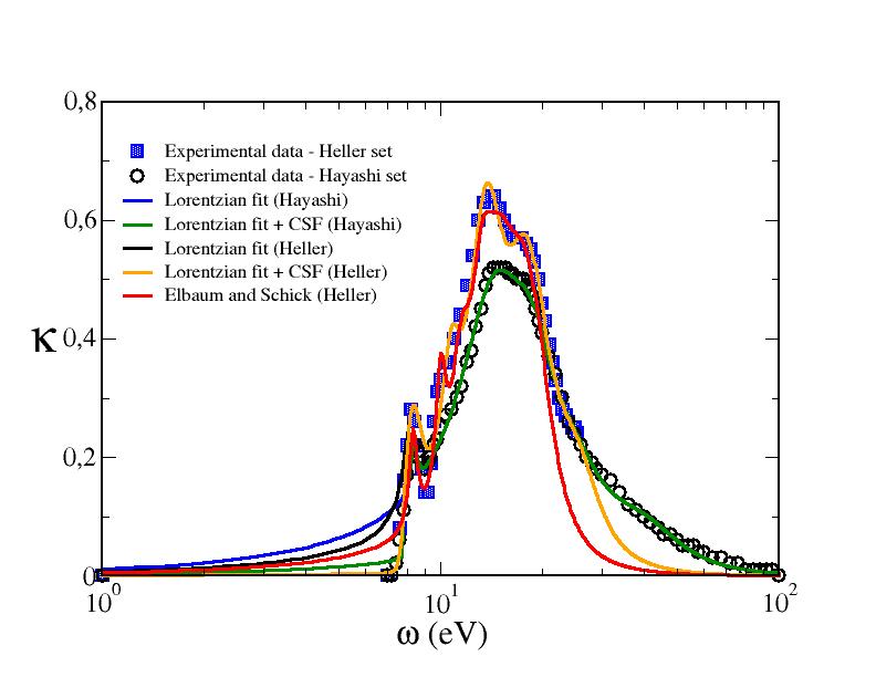
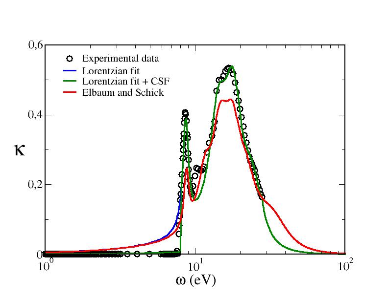
Figure 1: High energy band of the extinction index ($\kappa$). The figure compares experimental data (black dots) and parametric representations with Lorentzian oscillators (lines), as indicated in the legends. Experimental results for both water (top) and ice (bottom) are compared to the Lorentz model and the Lorentz-CSF model from this work. Fits of experimental data by ES are also displayed.

Unfortunately, despite these advantages, the model does not strictly obey the Kramers-Kronig relations, which is a physical constraint that dielectric functions must obey. It appears that to have a sharply decaying model that is accurate and obeys Kramers-Kronig one cannot avoid the use of special functions with no simple analytical form for $\epsilon(i\omega)$.[82] In practice, the deviations from Kramer-Kronig are very small. Fig. 2-top compares $\epsilon(i\omega)$ obtained in analytical form from Eq. (12), with the Kramers-Kronig transformation of the parametric representation of $\kappa(\omega)$ computed through its relation with $\epsilon_{1}(\omega)$ and $\epsilon_{2}(\omega)$. The two curves are clearly very similar on the scale of the figure and differ at most by 3%. In the same figure we also show the results obtained from the plain Lorentz model. The curves are almost identical for energies above the first electronic excitation, but differ significantly for lower energies. Thanks to the truncation of the Lorentz oscillators, the refractive indexes are now significantly lower and much closer to experimental results. For water, the Lorentz model at $\lambda=1000~{}nm$ provides a refractive index of 1.38, while the Lorentz+CSF model yields 1.34, far closer to the experimental value of 1.33 at 0 degrees.[83]

For ice, the Lorentz model yields 1.31, while the Lorentz+CSF model yields 1.29, to be compared with the experimental value of 1.30 at T=266 K.[47] These considerations provide confidence on our parametrization, particularly for the important region between the near IR and the soft x-rays (XR) regions. Innaccuracies could occur for the high energy tails beyond ca.40 eV, particularly for ice, because of lack of data, but these tails contribute little to the overall result of the Hamaker constant.

The results for the parametrization of dielectric properties of ice and water described here have been employed prior to publication in Ref.[38, 84]

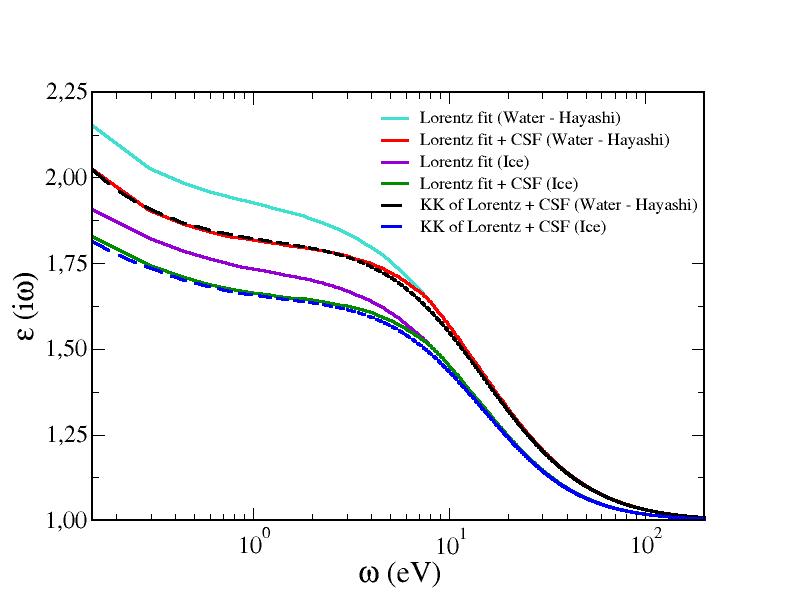
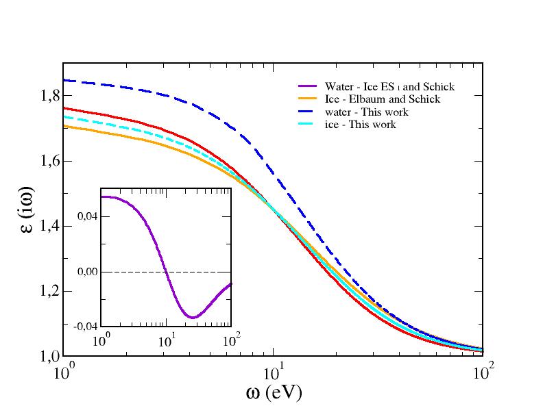
Figure 2: Dielectric response at imaginary frequencies of liquid water (Hayashi set) and ice. (Top) Black and blue dashed lines represent $\epsilon(i\omega)$ obtained from the KK relations over the parametric representation with CSF of $\kappa$ in this work. The accordance with their corresponding parametric representation of $\epsilon(i\omega)$ illustrates that although the model with CSF does not rigorously obey the Kramers-Kronig relation, it provides an accurate description of the dielectric response. (Bottom) A similar representation using the Heller set for water. The parametrization from ES predicts $\epsilon(i\omega)$ that is smaller for water than for ice at high energies. This is illustrated in the inset, where we plot the difference between the dielectric response of water and ice. In contrast, our revised parametrization of similar experimental data does not support that prediction and is positive all the way from MW to higher energies.

IV Results

We now use the fits for the complex dielectric function based on the Lorentz+CSF in order to calculate the Hamaker functions for a number of relevant interfaces involving water and ice. Unless otherwise stated, we describe the dielectric properties of water as obtained from fits to the Hayashi set.

IV.1 Interaction of water and ice across air

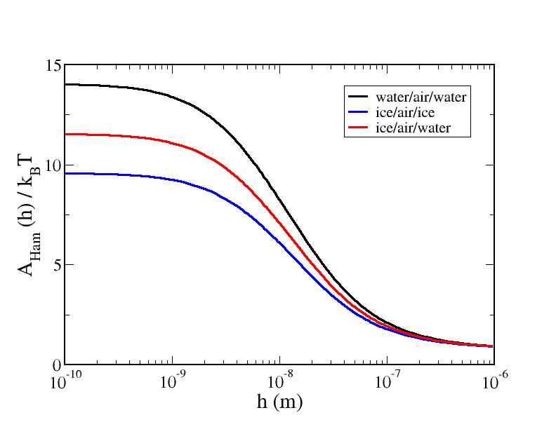
Figure 3: Hamaker coefficients of condensed water phases separated by air. Results are shown for water/air/water (black), ice/air/ice (blue) and ice/air/water (red). In all three cases, the Lorentz model + CSF of this work has been used, with the parameterization based on the Hayashi set for liquid water.

Whereas our main goal is the study of ice/water interfaces, we first consider the simpler systems that result from the interaction of either ice or water across air, i.e., water/air/water, ice/air/ice and ice/air/water. These cases pose less problems than systems where ice and water are in contact. According to DLP theory, Hamaker functions are given by differences of the form $(\epsilon_{i}-\epsilon_{m})$, with the index $i$ corresponding to media 1 or 2 interacting across medium $m$. Here, $m$ simply corresponds to air (or water vapor), and we can safely assume $\epsilon_{m}=1$. Accordingly, the Hamaker function is given by factors of the form $(\epsilon_{i}-1)$, which are positive at all frequencies. This implies that there could be some discrepancies on the actual value of the Hamaker function depending on the parametrization of dielectric properties, but there can be no controversy as regards its sign, which must always be positive (i.e. corresponding to attraction between two identical bodies across air).

Fig. 3 displays our results for the interaction of water-water, ice-ice and ice-water slabs. Of course, we find that the Hamaker functions are positive irrespective of the distance of separation, $h$, between the condensed media.

At small distances, $A(h)$ remains flat up to about 1 nm. The extrapolation of this function towards zero distance provides what is conventionally known as the Hamaker constant in the chemical physics literature.[76] A fact that is less often appreciated is that the Hamaker function gradually decreases as $h$ increases, and eventually adopts a much smaller constant value corresponding exactly to the $n=0$ contribution of the sum in Eq. (1) (c.f. Eq. (5)). i.e., whereas both in the limit $h\to 0$ and $h\to\infty$ the free energy follows the power law $g(h)\propto h^{-2}$, the corresponding proportionality coefficients are completely different. The former is set by the scale of the first electronic excitation, which usually falls in the ultraviolet region or beyond; the second one is of order $k_{B}T$, whence, usually two orders of magnitude smaller at ambient temperature.

This behavior may be rationalized by noting that the Hamaker function may be split into a static ($n=0$) and a frequency dependent contribution as $A(h)=A_{\omega=0}+A_{\omega>0}(h)$, with $A_{\omega=0}$, a constant of order $k_{B}T$:[76]

$$A_{\omega=0}=\frac{3}{4}\left[\frac{(\epsilon_{1}(0)-\epsilon_{m}(0))}{(\epsilon_{1}(0)+\epsilon_{m}(0))}\frac{(\epsilon_{2}(0)-\epsilon_{m}(0))}{(\epsilon_{2}(0)+\epsilon_{m}(0))}\right]k_{B}T$$ (15)

and $A_{\omega>0}(h)$, a function of $h$ which is finite at $h\to 0$ and vanishes at $h\to\infty$. Whereas this trend may not be obvious from direct inspection of either Eq. (1), or its simplified form, Eq. (5), we note that the limiting asymptotic behavior and the crossover from the $h\to 0$ and $h\to\infty$ regimes are described qualitatively by the approximate relation:[77]

$$\begin{array}[]{ccc}A_{\omega>0}(h)&=&\displaystyle{\frac{3\hbar c}{32\sqrt{2}\,n_{m}h}\left(\frac{n_{1}^{2}-n_{m}^{2}}{n_{1}^{2}+n_{m}^{2}}\frac{n_{2}^{2}-n_{m}^{2}}{n_{2}^{2}+n_{m}^{2}}\right)}\\ &&\\ &&\left[(2+\frac{3}{2}\nu_{T}h)e^{-\nu_{T}h}-(2+\nu_{\infty}h)e^{-\nu_{\infty}h}\right]\end{array}$$ (16)

where $\nu_{T}$ and $\nu_{\infty}$ are wave numbers that set the relevant length scales governing the behavior of $A(h)$. The first wave number, $\nu_{T}=4\epsilon_{m}^{1/2}\pi k_{B}T/\hbar c$ is known exactly. At water’s triple point, it falls in the near IR, and sets the length-scale where retardation effects become exponentially suppressed, $A_{\omega>0}\to 0$ and so $A(h)\to A_{\omega=0}$ for $h$ larger than the micrometer.

The second length-scale, $\nu_{\infty}$ is an empirical parameter that falls in the UV region and sets the crossover from the non-retarded regime, with interactions falling as $1/h^{2}$, to the retarded regime, where $A_{\omega>0}(h)$ becomes dominated by a decay of order $1/h^{3}$ (the Casimir regime). Generally, $\nu_{\infty}$ can be calculated numerically [38], but a good approximation is given by:[77, 85]

$$\nu_{\infty}=4n_{m}\frac{(n_{1}^{2}+n_{m}^{2})^{1/2}(n_{2}^{2}+n_{m}^{2})^{1/2}}{(n_{1}^{2}+n_{m}^{2})^{1/2}+(n_{2}^{2}+n_{m}^{2})^{1/2}}\frac{\omega_{e}}{c}$$ (17)

where $\omega_{e}$ is of the order of the principal electronic excitation, and $n_{i}$ is the refractive index of medium $i$.

For most practical matters, in the range of distances smaller than 1 nm, the Hamaker function might be approximated to a constant $A(0)$, which, for the interaction between either bulk water or ice slabs is of the order of a few tens of zJ (1 zJ$=10^{-21}\ J$).

IV.2 Interactions of the Ice/water/air system – Premelting

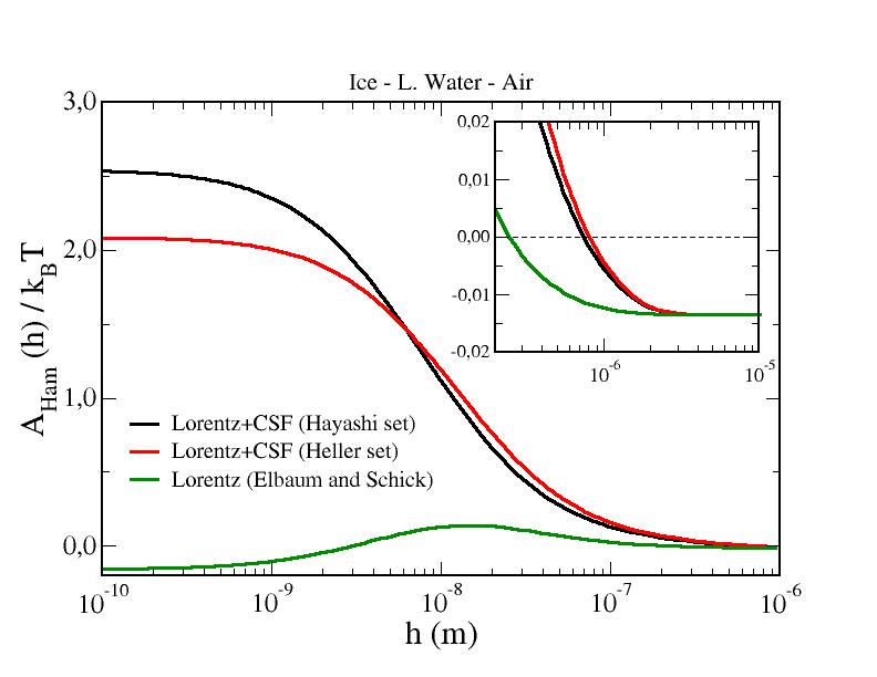
Figure 4: Hamaker coefficients for a premelting liquid film between ice and water. The figure shows result of the present work employing the dielectric function of liquid water from Hayashi (black) and Heller (red) sets. The green line displays the result of the ES parametrization for the Heller set. The inset shows the Hamaker function for premelting thickness in the scale of the micrometer.

We now turn to the more subtle problem of van der Waals interactions relevant to ice premelting. Here, we study how the surface free energy of a liquid film of water intruding between bulk ice and air depends on the liquid film thickness, $h$. In this case, the Hamaker function is dictated mainly by the difference between the dielectric functions of ice and water, which are very similar. Accordingly, not only the scale of the Hamaker function, but even its sign, depends crucially on an accurate estimation of the dielectric properties.

A look at Fig. 2 shows that in all the relevant range of the electromagnetic spectrum above the microwave region, the complex dielectric function at imaginary frequencies, $\epsilon(i\omega)$ is larger for water than it is for ice in our parametric representation, so that we can expect right away that the Hamaker function will be positive.

Fig. 4 displays the Hamaker function of ice/water/air system versus water layer thickness, and confirms this expectation. Results are shown for the water dielectric function as obtained from both the Hayashi and the Heller set, in order to account for possible uncertainty due to the choice of experimental dielectric properties. Although some differences are observed, we see that in both cases the Hamaker function is positive and presents a monotonic decay all the way from vanishing layer thickness to the micrometer range.

Again, the extrapolation of the Hamaker function to zero separation provides the Hamaker constant, which, in this case, is much smaller than that found for condensed water phases interacting across air, since the difference $\epsilon_{i}-\epsilon_{m}$, with $m$ corresponding to water, is now very small. Importantly, we also note that the Hamaker function starts to decrease significantly for thicknesses barely beyond the nanometer range. This behavior results from the large polarizability of the intervening phase between ice and air, i.e., water. Indeed, the value of $\nu_{\infty}$ in Eq. (16) may be estimated approximately from Eq. (17), whence, compared to the interaction between condensed water phases across air, we see that now $\nu_{\infty}$ increases by a factor of about $n_{w}$, implying a faster decay of the Hamaker function (c.f. Eq. (16)).

For water films thicker than 1 micrometer, Fig. 4 shows that the Hamaker function intersects the zero axis and becomes negative. This interesting behavior may be understood from Eq. (16), which shows that for distances larger than $\nu_{T}^{-1}$, $A_{\omega>0}(h)$ vanishes altogether, and only the $n=0$ term of the Hamaker function remains. Compared to contributions for $n>0$, this term has opposite sign, since the static dielectric function of ice is larger than that of water. As a result, van der Waals interactions oppose the growth of wetting films of small thickness, but favor growth of thick wetting films beyond the micrometer ($h>10~{}\mu~{}m$). It must be understood, however, that the intensity of van der Waals forces at such distances is extremely small, and whatever small perturbation, such as dissolved gases, electrolytes or minute changes away from the triple point could easily change the overall free energy balance.[86, 18]

Our predictions differ very much from the influential work of Elbaum and Schick, who first called the attention on the significance of van der Waals interactions in the study of ice premelting.[28] The Hamaker function predicted by these authors – Fig.4 (green lines) – is negative in the sub-nanometer range and positive in the nanometer range, then negative again at distances beyond the decade of micrometer.

The non-monotonic behavior predicted in Ref.[28] can be traced to the parametrization of the complex dielectric functions in that work, which predict $\epsilon(i\omega)$ that is larger for ice than for water at high energy, as seen in Fig. 2-bottom. However, we can see clearly in Fig. 1-top that the parametrization performed by ES fails to describe correctly the target high energy band of the Heller set. On the one hand, it appears to truncate the high energy tail in water’s extinction coefficient, and in the other hand, it exhibits too slow a decay for the same portion of the extinction coefficient of ice (i.e.. the high frequency range of $\epsilon(i\omega)$ in water is underestimated, while the corresponding portion in ice is overestimated), resulting in the complex dielectric function at imaginary frequencies which is larger for ice than it is for water. Such behavior does not appear to be supported by the current experimental data. Our revised parametrizations for ice and water (Heller set) using similar data as ES provide dielectric functions at imaginary frequencies that are always larger for water than for ice.

This result is in agreement with expectations from the f-sum rule and the Lorentz model of dielectric response.[87] At very high energies one expects a decay of the complex dielectric function of the form $\epsilon(i\omega)\propto\omega_{p}^{2}/\omega^{2}$, where $\omega_{p}\propto\rho_{e}$ is the plasma frequency and $\rho_{e}$ is the electron density in the material. Since the density of water is larger than that of ice, one expects that the plasma frequency should be larger for the former than it is for the latter, and accordingly, that $\epsilon(i\omega)$ should remain larger in water than in ice also at high energies.

In order to further clarify this problem, we calculated the optical properties of ice and water using Density Functional Theory. Previously, we showed that this theory does a good job at qualitatively describing the main differences in the absorption spectrum of ice and water in the region of electronic excitations. We use the Kramers-Kronig relations and the synthetic spectrum obtained from DFT in order to assess $\epsilon(i\omega)$ in an independent manner.

As a check of the theoretical calculations, we note that the predicted indexes of refraction are in fairly good agreement with experiment. For water, we obtain $n_{w}=1.31$, compared with the experimental value of $n_{w}=1.33$. For ice, DFT yields $n_{i}=1.28$, compared with the experimental value $n_{i}=1.30$. Whence, the refractive indexes are somewhat too low, but in the correct order.

The complex dielectric function at imaginary frequencies in the UV is displayed in Fig. 5, and it is seen that it remains higher for water than for ice in all the UV region and beyond, in agreement with expectations from the Lorentz model, and fits to the experimental results. In line with predictions of the refractive indexes, the $\epsilon(i\omega)$ differ very little, and provides a Hamaker functions that is about an order of magnitude smaller than predicted by the Lorentz-CSF fit. However, on qualitative grounds we see that the Hamaker function remains positive everywhere in the nanometer range.

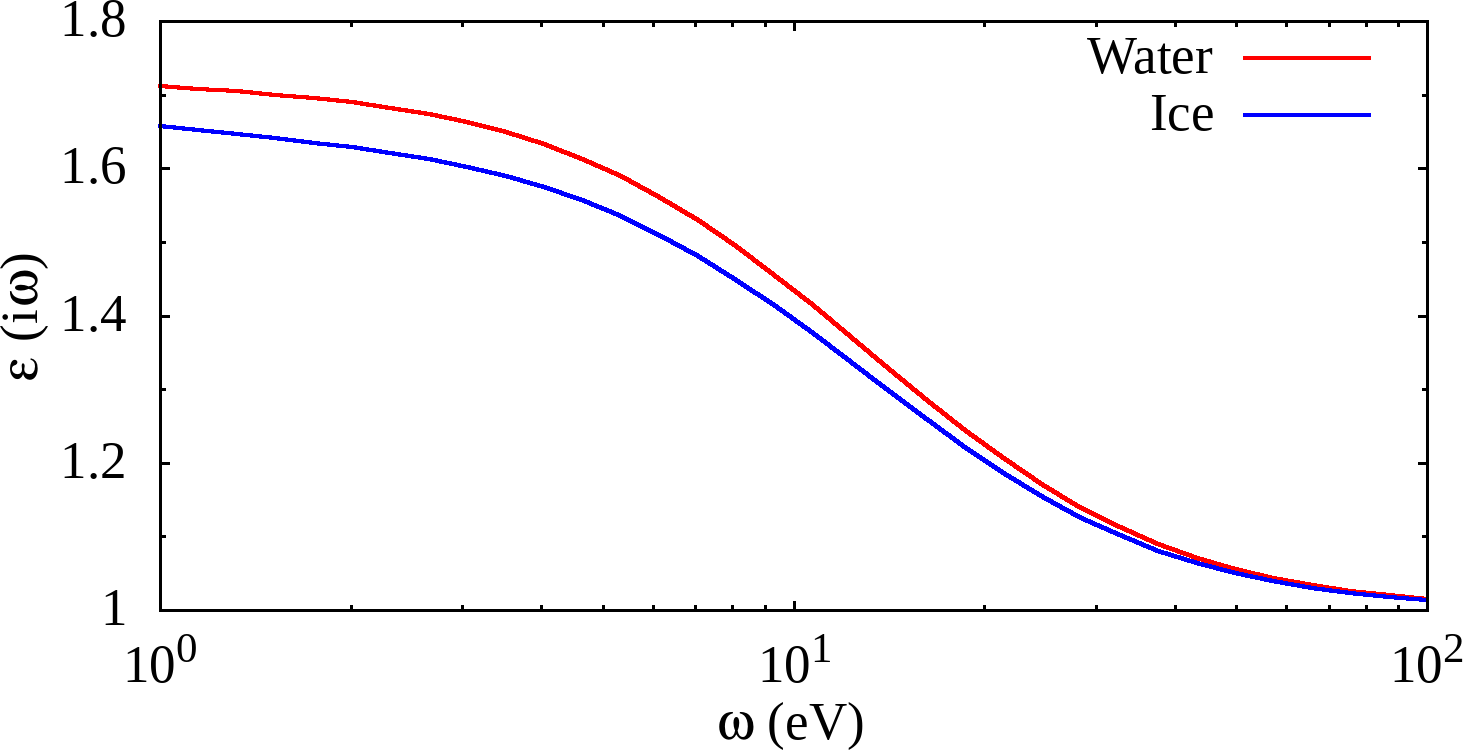
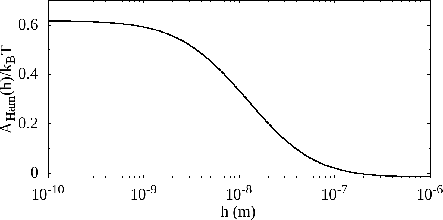
Figure 5: Dielectric response at imaginary frequencies of liquid water and ice computed in the DFT approximation(top). We can observe that the dielectric function of water remains always at bigger values than ice in the high energy region. This is in agreement with our new fits to the experimental data. Hamaker coefficients for a premelting liquid film between ice and water(bottom). The figure shows results of the calculations using the dielectric functions calculated in the DFT approximation.

In summary, we find that fits with a Lorentz model of two different experimental sets for the dielectric response of water, as well as theoretical DFT calculations predict an optical response in the ultraviolet region that is always higher for water than for ice, resulting in a positive Hamaker constant for the adsorption of a liquid water layer intervening between bulk ice and air.

IV.3 Implications for past work

From the discussion above, we see that the current improved understanding of the role of van der Waals forces on ice premelting differs qualitatively from the early predictions of Elbaum and Schick.[28] This work, henceforth referred as ES, has been very influential and the results used regularly on a number of studies,[88, 14, 89, 23, 90, 91] including work from some of us,[61, 92, 21] so we devote here a few lines to discuss how this could affect currently published results.

As far as physical implications are concerned, the ES model of van der Waals interaction predicts an interface potential with a minimum, implying incomplete surface melting. On the other hand, our work shows a negative monotonic contribution of van der Waals forces that completely inhibits surface premelting. Fortunately, the situation is not as bad as it appears. At short distances, the surface interactions are no longer dominated by van der Waals forces. Instead, they are governed by short range structural forces related to the packing of water molecules on the solid substrate.[93, 26, 27] Using a square gradient model together with molecular simulations of the mW model, Limmer and Chandler showed that at short range, packing effects promote surface melting.[23] The use of the mW model here is very convenient, because dispersion contributions are truncated at very short distances, so the results from this model can be used as a proxy of the effect of short range forces without any possible entanglement of long van der Waals tails. Similarly, in our recent work, we calculated the interface potential from simulations for the TIP4P/Ice model, and found clear evidence of a structural contribution promoting surface melting.[20, 21] Accordingly, as we will discuss in detail later, the addition of short range contributions to the van der Waals tail produces an interface potential with a minimum, in qualitative agreement with the findings of ES. It must be made clear, however, that the origin of this minimum does not stem from van der Waals forces alone, as implied by ES. It is a compromise between opposing short range structural forces and long range van der Waals forces.

IV.4 Interactions of the water/ice/air system – Surface freezing

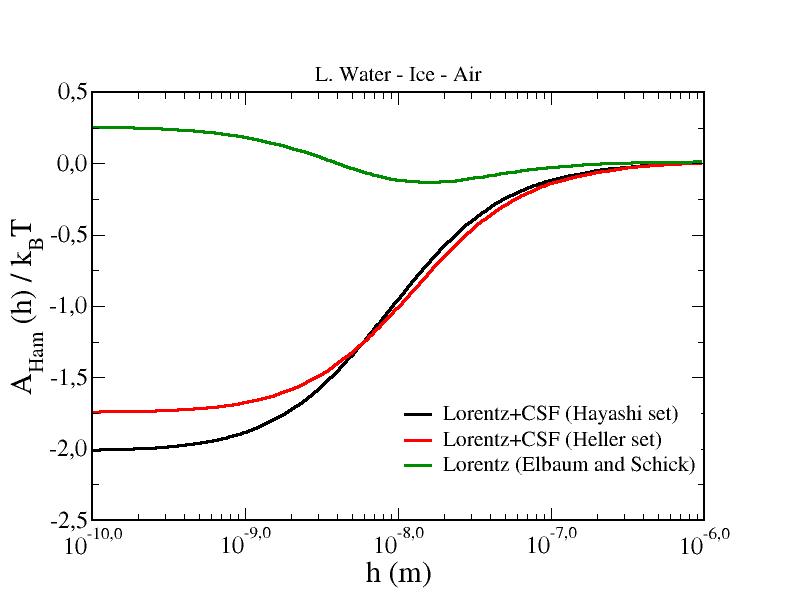
Figure 6: Hamaker coefficients from nanometers to microns compared to the thermal energy for water/ice/air. Black line and red line show the result of the present work employing, respectively, the dielectric function of liquid water with Hayashi and Heller sets. Green line displays the result of ES.

The parametrization used above for the dielectric functions of ice and water also allows us to study the free energy of ice films formed between bulk phases of water and air. The results obtained using either the Hayashi and the Heller sets are shown in Fig. 6. We see that the Hamaker function that results is negative in the relevant range between vanishing ice thickness down to the micrometer range, whereupon, it changes sign and becomes positive. In fact, the behavior observed in this case is nearly a mirror image of that observed for the ice/water/air system, since the interactions again are mainly governed by the difference $\epsilon_{w}-\epsilon_{i}$. i.e., the same factor governing the water/ice/air system, but with opposite sign.

This expectation is confirmed in Table 1, where we see that the Hamaker constant for the system water/ice/air is very similar, but of opposite sign than that of ice/water/air. As noted before, both are significantly smaller than the Hamaker constants for condensed phases of water across air. It is worth to remark that, although DFT computed values of the Hamaker constant result in sensibly smaller values in all cases, the relative order of the results and the order of magnitude is conserved.

Our results differ dramatically from expectations based on the ES parametrization, which yields instead a positive Hamaker constant, and thus, the prediction of complete suppression of surface freezing.[94]

system	w/a/w	i/a/i	i/a/w	i/w/a	w/i/a	i/w/i and w/i/w
A/zJ	52.77	36.07	43.46	9.54	-7.58	2.02
DFT	34.93	30.54	32.66	2.30	-2.12	0.19

Table 1: Table of Hamaker constants involving ice and liquid water as obtained from DLP theory with the parametrization of dielectric properties obtained in this work (using the Hayashi set to model water). Results are given in units of zJ=$10^{-21}$J

IV.5 Interactions across a condensed phase

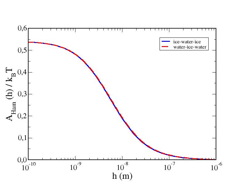
Figure 7: Hamaker function for ice/water/ice and water/ice/water as obtained from the Hayashi set. The continuous blue line corresponds to ice/water/ice and the dashed red line to water/ice/water.

As a final result, we now discuss the van der Waals forces when all the bodies involved are condensed phases, i.e., the interaction of two ice slabs with water in between (ice/water/ice), and the complementary case of two water slabs interacting across ice (water/ice/water). Since both of these settings refer to two identical interacting bodies across a third medium, van der Waals forces always conspire in favor of the two bulk materials to adhere, or, alternatively, the layer in between to vanish.

Figure 7 shows the Hamaker functions for both of these cases. As expected, the results are almost identical and the Hamaker function is always positive, implying attraction of the two bulk bodies. Because the intervening layer is a condensed phase, note that now the decay of the Hamaker function starts much sooner than in the case of two solids interacting across air. Particularly, we see that the Hamaker function has decayed by 10% already at a distance of 1 nm. Additionally, since all three bodies involved are condensed phases of water with similar refractive indexes, the Hamaker constant is now much smaller than in previous cases, $A_{ham}=2.02$ zJ. However, as long as the Hamaker function is positive, the two bulk materials will decrease their free energy by decreasing the thickness of the intermediate layer.

IV.6 Comparison with empirical force fields

Admittedly, the results for the Hamaker constants described above are obtained after rather involved numerical calculations within the framework of DLP theory, which accounts explicitly for polarization effects. An interesting question then is whether simple point charge molecular models that are widely used can possibly describe the apparently complex behavior embodied in DLP.

In practice, for non polarizable potentials interacting with the usual dispersion tail, $u_{ij}(r)\propto-C_{ij}/r^{-6}$, the Hamaker constant for the adsorption of phase $m$ at the interface between phase, $1$, and phase $3$ may be estimated accurately from a plain sharp-kink approximation of the density profiles as:[95, 96, 97]

$$A_{1m3}=4\pi^{2}(C^{1/2}_{11}\rho_{1}-C^{1/2}_{mm}\rho_{m})(C^{1/2}_{33}\rho_{3}-C^{1/2}_{mm}\rho_{m})$$ (18)

where $\rho_{i}$ are bulk number densities of the phases involved, and we have assumed $C_{ij}=C_{ii}^{1/2}C_{jj}^{1/2}$.

In the case of interest here, a single component system at the triple point, all phases are formed from water, so that all $C_{ii}=C$. In most point charge models, the contribution of electronic polarizabilities to the constant $C$ is described as $C=4\epsilon\sigma^{6}$, with $\epsilon$ and $\sigma$ the usual Lennard-Jones parameters (an additional Keesom like term that has been neglected here contributes to the $n=0$ static term only). Whence, the electronic Hamaker constant for the growth of a water film in between ice and vapor simplifies to:[61]

$$A^{e}_{iwa}=4\pi^{2}\epsilon\sigma^{6}(\rho_{v}-\rho_{w})(\rho_{i}-\rho_{w})$$ (19)

where the superscript emphasizes that this expression accounts only for dispersion interactions due to electronic polarizabilities. Since the density of ice is smaller than that of water, we find readily that $A^{e}_{wia}>0$, in agreement with the far more involved DLP theory. For the related system of ice growing between liquid water and air, the Hamaker function is the same as above, albeit with the interchange of ice and water labels. Accordingly, we find exactly the same result, but with opposite sign, which is also consistent with results from DLP theory.

Eq. (18)-19 above show that the positive sign of $A_{iwa}$ results from the fact that $\rho_{i}<\rho_{w}$, so that the absence of complete surface premelting in ice is actually one more of water’s anomalies, a result in agreement with expectations by Nozieres,[98] but at odds with claims by Fukuta.[99] On the contrary, noble gases such as Neon and Argon, where the solid density is larger than that of the liquid phase, exhibit surface melting. The result of Eq. (19), firmly rooted in the theory of wetting,[95, 96] contrasts with attempts to determine intermolecular forces in premelting films with no account of density differences between the involved phases.[99, 100]

A compilation of the electronic Hamaker constants for interactions involving ice, water and air obtained from Eq. (18) for different non-polarizable water models are shown in table 2.[68, 69, 70, 71, 72]. The results are compared with predictions from DLP theory. The electronic Hamaker constants from DLP are calculated using the parametrized dielectric response stemming from electronic contributions only (i.e., oscillators with absorption frequencies larger than the near IR.

For interactions of condensed water phases across air, Table 2 shows that the old generation of water models (TIP4P and SPC/E) appear to perform rather well, with values of electronic Hamaker constants rather close to predictions from DLP theory. Surprisingly, the new generation of force fields appear to overestimate considerably the dispersion interactions, with TIP4P/2005 performing significantly better than TIP4P/Ice and TIP4P-D. On the other hand, for interactions between a condensed phase and air (ice/water/air and water/ice/air), all force fields predict interactions that are too weak compared with DLP.

model	TIP4P	SPC/E	TIP4P/2005	TIP4P/Ice	TIP4P-D	DLP
$A_{iwa}^{e}/$ zJ	3.83	3.92	4.62	5.33	5.65	9.57
$A_{wia}^{e}/$ zJ	-3.52	-3.63	-4.24	-4.90	-5.19	-7.59
$A_{waw}^{e}/$ zJ	46.7	47.9	56.3	65.04	68.8	49.1
$A_{iai}^{e}/$ zJ	39.3	40.4	47.4	54.8	58.0	32.4
$A_{iaw}^{e}/$ zJ	42.8	44.0	51.7	59.7	63.2	39.8

Table 2: Electronic contribution to Hamaker constants in point-charge models. Results for the models are obtained using Eq. (19), with densities evaluated at the experimental triple point of water.

The direction for improvement of force field based on this comparison appears to be to keep Lennard-Jones parameters similar to those of TIP4P, but with an increased dipole moment. This is roughly the direction taken in the development of TIP4P/2005. Of course, a quantitative comparison between DLP cannot be taken too far, because electronic and dipolar terms in empirical force fields are not fully meaningful, and the DLP predictions are also somewhat subject to uncertainties of the dielectric parametrization.

However, it is pleasing to find that currently accepted force fields appear to provide a correct qualitative description of surface dispersion forces. Based on this observation, we expect that the long range behavior of the interface potential predicted by empirical models used in our recent work is a reliable proxy for the physics of premelting films.[61, 20, 63]

V Discussion

Having settled the role of van der Waals forces on the interface potential we are now on good position to discuss the important problems of surface melting, regelation and surface freezing.

V.1 Surface premelting

In the case of surface premelting, the surface free energy of the ice/vapor interface as mediated by a premelting film of thickness $h$, is given by:

$$\omega_{iv}(h)=\gamma_{iw}+\gamma_{wv}+g(h)$$ (20)

where $g(h)$ is the interface potential describing the free energy cost of a premelting film as a function of film thickness. In the limit that $h\to\infty$, $g(h)=0$, and the surface free energy is just the sum of ice/water and water/vapor surface tensions.

The equilibrium value of the film thickness, $h_{e}$ is obtained by minimization of the free energy, $\omega_{iv}(h)$, such that $dg(h)/dh=0$, whereupon, one obtains the equilibrium interface tension of the ice/vapor interface as:

$$\gamma_{iv}=\omega_{iv}(h_{e})$$ (21)

This result acknowledges explicitly the fact that the ice/vapor surface tension may be mediated by a finite premelting film of adsorbed water. Of course, its properties need not be exactly as those of bulk water.

Three different situations are possible. The first corresponds to the case where the absolute minimum of $g(h)$ occurs at $h=0$. In that case, the structure of the ice/vapor interface would be that of a perfectly terminated ice slab in contact with air. The second one occurs in the opposite situation, where the absolute minimum is at $h\to\infty$. In that case, $g(h)\to 0$ by construction, so that $\gamma_{iv}=\gamma_{iw}+\gamma_{wv}$ exactly. This equality is the condition for wetting of the ice/vapor interface by an intruding macroscopic film of liquid water, which in this case is known also as surface melting. Finally, a third situation can arise if an absolute minimum of $g(h)$ exists for finite values of $h_{e}$. This is a situation of incomplete melting, whereby the equilibrium ice/vapor interface is mediated by a stable premelting film of finite thickness.

Based on the calculations of the previous section, we see that $g_{vdw}(h)$ is a monotonic and negative function, with an absolute minimum at $h=0$. Accordingly, we confirm, in agreement with recent work and unpublished results by ourselves,[35, 36, 37, 38, 84] that van der Waals forces conspire against the surface premelting of ice, favoring a perfectly terminated ice/vapor surface instead.

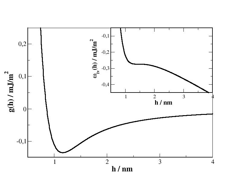
Figure 8: Interface potential for ice premelting suggested in this work. Notice the model is valid for crystal planes above their roughening transition. Inset: The corresponding surface free energy at the surface spinodal vapor pressure becomes unstable and the premelting film thereof undergoes complete wetting of the underlying ice substrate.

In practice, DLP theory is not accurate in the limit of $h\to 0$, because it assumes structureless interfaces (this can be readily understood without any acquaintance of DLP, merely by noticing that its only input are bulk dielectric properties). At short range, $g(h)$ is dominated by interactions arising from the distortion of the bulk density profile, which, at low temperatures decays on the scale of the molecular diameter. Therefore, the full interface potential is expressed as:

$$g(h)=g_{sr}(h)+g_{vdw}(h)$$ (22)

Here, $g_{sr}(h)$ is the short range contribution. For ice premelting, we have recently showed that the qualitative behavior of this term follows expectations from liquid state theory,[25, 26] and may be described as:[20]

$$g_{sr}(h)=B_{2}\exp(-\kappa_{2}h)-B_{1}\exp(-\kappa_{1}h)\cos(q_{o}h+\phi)$$ (23)

where $B_{i}$ are positive constants; $\kappa_{i}$ are inverse decay lengths, $q_{o}$ is dictated by the wave-length of packing correlations in the liquid (i.e. the maximum of the liquid’s structure factor) and $\phi$ is the phase. This relation improves the result of field theory, which provides just the first term of the right hand side, but shares, in common with the above result the expectations that $B_{2}>0$.[22, 23]

The actual value of the parameters depends somewhat on the ice facet, but a common feature they all share is that $B_{2}$ is significantly larger than $B_{1}$. This implies that for film thicknesses on the order of $\kappa_{2}^{-1}$, $g_{sr}(h)$ is positive,[23] while the oscillatory term could make $g_{sr}(h)$ negative at larger distances provided $\kappa_{1}<\kappa_{2}$, a condition that is expected to hold only for faces below their roughening transition.[25, 20] At the triple point, only the basal face meets this condition.

Overall, it follows that at short range, packing correlations repel the liquid-vapor interface away from the solid substrate, promoting surface melting; at long range, van der Waals forces bind the liquid-vapor interface, and inhibit the build up of a large liquid film. Therefore, the interface potential must display an absolute minimum of negative energy at intermediate thicknesses, such that $g(h_{e})<0$, and the ice surface thus exhibits a liquid premelting film of finite thickness at the triple point. Accordingly, from Eq. (20) and Eq. (21), we see that $\gamma_{iv}<\gamma_{iw}+\gamma_{wv}$. i.e., water does not wet ice at the triple point, and must form liquid droplets of finite contact angle, in agreement with recurrent reports in the literature.[101, 102, 17, 86, 103, 104] The presence of the oscillatory term in Eq. (23) means that there could be an additional shallow minima at larger thickness in the basal facet, thus explaining the existence of two different incomplete wetting states that have been reported in experiments.[104]

Our considerations differ with the qualitative model of interfacial forces suggested in Ref.[104]. These authors observed growth and spread of steps and terraces on the basal facet of ice, and argued that the presence of steps must imply a smooth surface inconsistent with a highly disordered premelting layer. Accordingly, they hypothesized an interface potential with an absolute minimum at $h=0$, implying a bare ice surface as the stable state of the basal face. However, we have shown using both theoretical models and computer simulations that a smooth facet with steps can exist even in the presence of a premelting film,[60, 61, 20, 21] such that our theoretical model of the interface potential and the experimental observation of steps and terraces are mutually consistent.

A simplified qualitative form of the interface potential, adequate in the region $g(h)<0$ that characterizes the primary minimum may be obtained from the leading term of Eq. (23) and the non-retarded van der Waals contribution:

$$g(h)=Be^{-\kappa h}-\frac{A_{iwa}(0)}{12\pi h^{2}}$$ (24)

This result is of the same form as anticipated by Limmer and Chandler,[23] but notice that our results show the positive sign of the Hamaker constant $A_{iwa}(0)$ stems mainly from high frequency contributions of the dielectric response (rather than from the static term).

This simple model of interface potential allow us to clarify many of the speculations on surface melting discussed in the literature,[9, 105, 106, 107, 11, 12, 13, 14, 15, 16] as well as our own.[61]

Using our estimates for the Hamaker constant in table 1, together with $B=0.07$ J/m² and $\kappa=6.2~{}nm^{-1}$ obtained for the prism facet in our previous work,[20], we find a free energy minimum of $g(h_{e})=-0.135$ mJ$/$m², and an equilibrium film thickness of barely $h_{e}\approx 1.16$ nm. The presence of this thin premelting film is not in conflict with the formation of liquid droplets (c.f. Ref.[108, 100]). By plugging Eq. (21) into Young’s equation, $\gamma_{iv}=\gamma_{iw}+\gamma_{wv}\cos\theta$, we find that the shallow minimum of the interface potential provides:

$$\cos\theta=1+\frac{g(h_{e})}{\gamma_{wv}}$$ (25)

Using our model interface potential into this formula, together with $\gamma_{wv}=75.7$ mJ$/$m²,[109] we predict a contact angle of $\theta=3.4^{\circ}$. For comparison, first experimental measures of about 12^o,[101] have thereafter been revised to smaller than 5^o,[102] with estimates of 2^o,[86, 104] or even less than 1^o depending on the ice facet.[110, 86]

These considerations are relevant exactly at the triple point, where ice, water and vapor have all exactly the same chemical potential, so that one phase can grow from the other at free cost. As soon as one moves away from the triple point, the formation of the premelting film picks an extra free energy cost, and the free energy in Eq. (20) becomes:

$$\omega_{iv}(h)=\gamma_{iw}+\gamma_{wv}+g(h)-\Delta p_{wv}(\mu)h$$ (26)

where $\Delta p_{wv}$ is the difference between bulk liquid and vapor pressures at the system’s chemical potential. Assuming that the vapor sets the total chemical potential, as is usual in experiments, we can estimate this as $\Delta p_{wv}=\rho_{w}k_{B}T\ln p/p_{wv}(T)$, where $p$ is the imposed vapor pressure, $\rho_{w}$ is the bulk liquid density and $p_{wv}(T)$ is the water-vapor saturation pressure at the systems temperature. Whence, as the vapor pressure $p$ is raised above $p_{wv}$, the free energy $\omega_{iv}(h)$ picks a linear term proportional to $h$, and the equilibrium film thickness is displaced to larger values of the film thickness. Assuming a metastable equilibrium of ice with supersaturated vapor (this can be achieved for very small growth rates of ice close to the triple point, c.f. 21), the film thickness may be obtained by extremalization of the above equation. This leads readily to an expression for the vapor pressure in equilibrium with a quasi-liquid layer of thickness $h$:[20]

$$p=p_{wv}(T)e^{-\frac{\Pi(h)}{\rho_{w}k_{B}T}}$$ (27)

where $\Pi(h)=-dg(h)/dh$ is the disjoining pressure.[93, 27] i.e., as $h$ increases, $\Pi(h)$ becomes more negative, and the vapor pressure in equilibrium with the premelting film increases.

Eventually, however, $\Delta p_{wv}$ is sufficiently large that the linear term in Eq. (26) washes out completely the minimum of the interface potential. This corresponds to the limit where the disjoining pressure attains its absolute minimum. i.e. a spinodal point is reached and a premelting film can no longer be stabilized.

Using our model potential, we find for the spinodal limit of the premelting film $h_{sp}=1.44$ nm, which corresponds to a disjoining pressure of $\Pi(h_{sp})=-1.12$ bar. Whence, the maximum vapor pressure than can be attained before the ice surface becomes wet is estimated from Eq. (27) as $p_{sp}\approx 1.0009p_{wv}(T)$. This explains why experiments often report very thick wetting films close to the triple point. As soon as the vapor pressure is slightly above the liquid-vapor coexistence curve, the premelting film becomes unstable and can grow without bounds on top of the bulk ice. For temperatures close to the triple point, this requires an exquisite control of the vapor pressure. Once the spinodal is traversed, ice grown from vapor actually freezes from the condensed wetting film that lies above.[21]

In practice, both vapor condensation and ice growth occur simultaneously.[105, 107, 111, 112] This results in an increase of the actual spinodal pressure in a complicated manner that depends on the precise growth mechanism.[21] Accordingly, our calculation based on Eq. (27) provide a lower estimate of the pressure where premelting films become unstable.

Eq. (27) does become exact at thermodynamic equilibrium, which is strictly realized for ice in contact with vapor along the sublimation line, such that $p$ is equal to the saturation pressure of vapor over ice, $p_{iv}$. In this limit, using Clausius-Clapeyron, we find that $\Delta p_{iv}=\frac{\rho_{w}\Delta H_{iw}}{T_{t}}(T-T_{t})$, leading to the well known result for the premelting thickness as a function of temperature along the sublimation line:[14]

$$\frac{\rho_{w}\Delta H_{iw}}{T_{t}}(T-T_{t})=\Pi(h)$$ (28)

Accordingly, at the triple point the condition of equilibrium is the vanishing of $\Pi(h)$. In the absence of a binding term in the disjoining pressure, as often assumed,[16] this condition is met only for $h\to\infty$. However, because of the van der Waals contribution, the condition of vanishing disjoining pressure is met at a finite equilibrium film thickness $h_{e}$ corresponding to the minimum of the interface potential $g(h)$.

Our results for the surface free energy of the equilibrium ice/vapor interface (i.e., with a mediated premelting film), allow us to answer a general question relevant in atmospheric physics. Consider one has at some low temperature a bulk ice phase in equilibrium with its vapor, and gradually increases the temperature along the ice-vapor coexistence line up to the triple point. In that moment, all three phases have exactly the same bulk free energy per molecule, and the only factor inhibiting the condensation of a bulk water phase is the surface free energy. The question then is posed, where will a bulk flat phase grow preferentially? Will it be within the bulk vapor phase, within the bulk ice phase or intruding into the ice/vapor interface? To solve this, recall that the equality of bulk free energies imposed at the triple point requires one to assume the interfaces that are formed have strictly zero curvature. Therefore, we refer here to the formation of bulk flat phases, parallel to the current ice/vapor interface. The formation of a macroscopic water phase within the vapor will then cost $2\gamma_{wv}$ per unit surface. Similarly, the formation of the water phase within the bulk ice phase will require $2\gamma_{iw}$. If, on the other hand, the bulk water phase forms at the ice/vapor interface, the cost is $\gamma_{iw}+\gamma_{wv}-\gamma_{iv}$. Bearing in mind approximate estimates of the surface free energies of ca. $\gamma_{iv}>\gamma_{wv}>\gamma_{iw}$, we readily rule out the formation of water within the vapor phase. Furthermore, recalling from Eq. (20)-21 that $-\gamma_{iv}=\gamma_{iw}+\gamma_{wv}+g(h_{e})$, we see that the formation of condensed water at the ice/vapor interface will cost $-g(h_{e})$, which barely amounts to $1.35\times 10^{-4}$ J/m ², much less than any of the other cases. So if a large macroscopic condensed water phase is to form, it will grow in between ice and vapor. However, the state of minimal free energy is in fact a bulk ice phase coexisting with a finite film of equilibrium thickness $h_{e}$ between a bulk vapor phase. Accordingly, the melting of a perfect ice monocrystal is actually a weakly activated process, as postulated by Knight many years ago,[102] and is actually the expected situation for materials with incomplete surface premelting.[12, 113] However, our discussion above shows that it will suffice to increase the pressure barely a few Pascal above the triple phase for the macroscopic bulk water phase to become the preferred state.

V.2 Regelation

Describing a famous experiment,[114] Faraday noted that ”two pieces of thawing ice, if put together, adhere and become one”. This and some other observations helped formulate the hypothesis of ice premelting for the first time, despite great difficulties to understand how freezing could occur in regions of the bulk phase diagram where water is the preferred phase.[9]

In this regard, notice however that van der Waals forces always conspire in favor of two equal bulk materials to adhere. In this case, assuming ice is covered with a premelting layer, and two such ice samples are brought together, a liquid bridge between the ice slabs will form spontaneously. In conditions favoring water over vapor, i.e. above the liquid-vapor coexistence curve, water will not evaporate. However, the liquid layer can vanish by freezing, since, as described in the previous section, interactions in an ice/water/ice system favor attraction of the bulk bodies. i.e.: shrinking of the intervening liquid layer by freezing.

In practice, because the involved Hamaker constants are rather small, the process is mainly driven by bulk and surface free energies, rather than by the van der Waals forces. In the language of wetting physics it may be described essentially as a phenomenon of capillary freezing.

To be more specific, consider two large spherical ice balls, of radius $R$. Then, the force of attraction between the balls will be given, according to the Derjaguin approximation,[76] by $F(d)=\pi R(\omega_{i}(d)-\omega_{v}(\infty))$, where $\omega_{i}(d)$ is the free energy of the ice bridge joining two planar bulk ice slabs, and $\omega_{v}(\infty)$ is the free energy of two planar ice slabs separated by a macroscopic bulk vapor phase. The former is just the bulk free energy of forming ice from the vapor, $\omega_{i}(d)=-\Delta p_{iv}d$. The latter is the cost of the two isolated ice/vapor interfaces, $\omega_{v}(\infty)=2\omega_{iv}(h_{e})$, with $h_{e}$, the equilibrium layer thickness at ambient pressure as dictated by minimization of Eq. (26). Whence, the total free energy cost of forming the ice bridge is:

$$F(d)=2\pi R[\Delta p_{wv}h_{e}-\frac{1}{2}\Delta p_{iv}d-\gamma_{iw}-\gamma_{wv}-g(h_{e})]$$ (29)

We see that at the triple point, where $\Delta p_{wv}=\Delta p_{iv}=0$, the formation of an ice bridge is a favorable process that is driven by the surface free energies.

In order to show why regelation occurs exceptionally for ice, let us simplify the problem and choose quite naturally a bridge length $d=2h_{e}$. Then, assuming the vapor is an ideal gas, and taking into account Clausius-Clapeyron, we find that the condition for the formation of an ice bridge as a function of vapor pressure and temperature is:

$$\ln\frac{p}{p_{t}}\leq\frac{\gamma_{iw}+\gamma_{wv}}{k_{B}T(\rho_{w}-\rho_{i})h_{e}}+\frac{\rho_{i}\Delta H_{iv}-\rho_{w}\Delta H_{lv}}{(\rho_{w}-\rho_{i})}\left(\frac{1}{T}-\frac{1}{T_{t}}\right)$$ (30)

Due to the anomalous properties of ice, $\rho_{w}>\rho_{i}$, the first term in the right hand side is positive. This means that, at $T=T_{t}$, where the second term vanishes, the inequality can be met even at $p/p_{t}>1$. i.e., an ice bridge can form in conditions where the liquid is the preferred phase. Or in Faraday’s own words ”at a place were liquefaction was proceeding, congelation suddenly occurs”.[114]

On the contrary, for ordinary materials, where the density of the solid phase is larger than that of the liquid phase, this term is negative. Whence, the ice bridge could form at pressures $p/p_{t}<1$. However, at $T=T_{t}$ and $p<p_{t}$, the solid does not exhibit a noticeable premelting layer, because it is found in a region of the phase diagram where the bulk liquid phase is not favored, i.e. sublimation occurs instead (recall the slope of the melting curve is positive for the usual case of solid density larger than that of liquid). Therefore, the kinetics of regelation is much slower in this case, since the bridge must form from the vapor phase, rather than from a premelting layer.

As regards the famous controversy between Faraday and Thomson on the origin of regelation,[114, 115] we see that both surface premelting and the negative slope of the melting line play a role in the overall free energy balance embodied in Eq. (30), but pressure melting is not required for regelation to occur. The capillary freezing described here, however, refers to the regelation between two parcels of ice at atmospheric pressure as considered by Faraday,[114] which can be very different from the regelation mechanism invoked to explain glacier motion and wire regelation.[14, 116]

As a final remark we note that in the region of higher pressures where the condition of capillary freezing is satisfied, Eq. (30), it actually becomes more favorable for plain capillary condensation to occur. Bearing this in mind one finds that the stricter condition for regelation (i.e., such that an ice bridge is more favorable than a liquid bridge) satisfies Eq. (30) with the term $\gamma_{iw}+\gamma_{wv}$ replaced by $\gamma_{iw}$ alone.

V.3 Surface freezing

It is a matter of everyday experience that large ice crystals form on the surface of water. Similar observations may be made experimentally for small but fully nucleated crystals of mm size.[117] Such observations are easily explained from buoyancy. However, some experiments and theoretical studies have suggested that tiny crystals might not actually reach the surface as a result of buoyancy, but are actually nucleated in-situ at the liquid-vapor interface.[64, 65] i.e., that the liquid-vapor interface could promote the nucleation of ice by orders of magnitude compared to bulk.[66, 67]

The problem again is one of wetting physics: we consider the growth of an ice film at a liquid-vapor interface at coexistence as the system is cooled down to the triple point. A bulk planar phase could then be formed with the same bulk free energy cost as the vapor and liquid. Creating bulk ice in the midst of the vapor phase costs $2\gamma_{iv}$; the cost of creating the same phase within bulk water costs $2\gamma_{iw}$; while growing ice in between air and water has a cost of $\gamma_{iw}+\gamma_{iv}-\gamma_{wv}$. But again, because the equilibrium ice-air interface is actually covered by a premelting film, use of Eq. 20-21 shows that the total energy cost of growing the bulk ice phase between bulk water and vapor phases is just $g(h_{e})<0$. Therefore, our calculations confirm that it is favorable for ice to grow at the water-vapor interface among all other choices. Bear in mind that this does not mean actually strict ’surface freezing’, understood as the formation of ice atop the liquid-vapor surface. Instead, because the ice-vapor surface that is formed is covered by a premelting layer, the actual picture is that of a bulk ice phase formed at a distance $h_{e}$ below water. However, this occurs only in a very small range of vapor pressures. Indeed, since the premelting film is destabilized and grows unbounded as soon as the pressure is larger than the surface spinodal pressure, saturating the interface above $p_{s}\approx 1.0009p_{wv}(T)$ will promote condensation of water and ice would then be buried by a thick water film. Eventually, if the ice volume is large enough, it will experience buoyancy forces, and the final outcome is the result of a balance between surface interactions and the bulk buoyancy force.[91]

VI Conclusions

In this work we have combined results from wetting physics, quantum Density Functional Theory and Lifshitz theory of van der Waals forces in order to assess the role of molecular interactions at a number of relevant interfaces involving ice and liquid water.

For the long standing problem of ice premelting,[9, 10, 11, 12, 13, 14, 15, 16] our results show that van der Waals forces inhibit the growth of thick liquid films and prevent ice from surface melting. On the contrary, short range structural forces promote wetting. The balance between these competing forces results in a finite equilibrium premelting thickness on the order of the nanometer. Our theoretical results are consistent with computer simulations,[118, 119, 111, 120, 121, 122, 62, 20, 63] and a large body of widely different experimental techniques.[123, 124, 125, 126]

Combining our model of intermolecular forces with results of wetting physics, we are able to assess the role of vapor pressure on the premelting behavior. Our results show that the premelting layer can become unstable by increasing the vapor pressure just a few Pascal above water-vapor saturation. This implies that unless an exquisite pressure control is exercised, ice will readily surface melt in a water supersaturated atmosphere. This adds an additional mechanism for surface melting apart from impurities,[18] and explains recurrent observations of very thick wetting layers (c.f. [11, 15]). We believe this finding is particularly significant for studies of atmospheric ice, including ice growth and gas adsorption.[3]

Our results also provide insight into the related problem of surface freezing. We show that the most stable site for ice to nucleate at under-saturation is immersed at a distance of roughly one nanometer below the water-vapor interface, in agreement with suggestions and recent simulation studies.[64, 65, 66, 67] However, increasing saturation above the water-vapor coexistence line promotes the growth of a thick wetting film above ice. As a result the surface enhancement effect on ice nucleation is lost in a supersaturated atmosphere.

Finally, we show that the property of ice regelation, understood as the ability of thawing ice parcels to adhere by freezing can be described as a process of capillary freezing at conditions in the phase diagram where liquid water is the preferred phase.

We have shown that all of these observations –incomplete premelting, enhanced subsurface nucleation and regelation of thawing ice– have their origin in the negative slope of the freezing line and can therefore be added to the large list of water anomalies.

Supplementary Material

See supplementary material for details on modeling dielectric functions; details on DFT methodology; and tables with parameters.

Author Information

Contributions

J.L.M. modeled dielectric functions and calculated van der Waals forces. F.I.R. performed DFT calculations. L.G.M. interpreted results and wrote manuscript.

Corresponding author

Correspondence to: lgmac@quim.ucm.es

Supplementary Material

Intermolecular forces at ice and water interfaces: premelting, surface freezing and regelation.

Juan Luengo-Márquez, Fernando Izquierdo-Ruiz, and Luis G. MacDowell

Appendix A Modeling the dielectric functions

The dielectric function of a material may be obtained from the refractive index or the extinction coefficient.[29, 87] Measurements of the refractive index are suitable in regions were no absorption takes place, while extinction coefficients are measured more accurately in regions of the spectrum with high absorption. Here, we will parametrize our model from data of extinction coefficients, available for water and ice in all the relevant region of the spectrum, but will gauge or model against the refractive index in the near infrared (IR). A summary of current parametrizations for the spectrum of water is presented in Table 3. In the following, we review sources of literature data for the optical properties in order to select an optimal data set for the purpose of modeling optical properties of water and ice in the neighborhood of the triple point.

Reference	Description
Parsegian and Weiss[30]	First accurate fit to UV band by Heller, with a microwave term and five IR absorbtions.
Elbaum and Schick[28]	Uses similar data as [30], but high energy band is underestimated.
Roth and Lenhoff[31]	Uses the same MW and IR data than parsegian and Weiss, but improves the parametrization of the Heller UV band considerably.
Dagastine et al.[32]	Uses improved data in the IR region and obtains the dielectric function at imaginary frequencies from a KK analysis.
Fernandez-Varea et al.[33]	Uses the accurate representation of the Heller data, enforcing the f-sum rule.
Wang and Nguyen[34]	Full update of the UV data using results from Ref.[45], but does not provide results for the IR region and uses KK analysis with epsilon(iw) in tabulated form.
Fiedler et al.[37]	Improved parametrization with detailed study of MW and far IR regions, but overestimates refractive index.
Gudarzi and Aboutalebi[39]	Uses the Hayashi band, with high energy decay estimated with f-sum rule and enforcement of refractive index, but parametric form at low energy based on room temperature results.

Table 3: Review of optical properties of water parametrized for use in Hamaker coefficient calculations.

A.1 Water

A.1.1 From the microwave to the visible region

In this low energy region, ranging from $10^{-3}$ eV to about 1 eV, the spectrum of water exhibits significant absorption all the way from the MW, across the IR, and to the mid-IR, with most of the vibrational transitions ending sharply at ca. 0.4 eV. The remaining range of the spectrum including the visible (VIS), exhibits very small absorption and an almost constant refractive index, ca. $n=1.33$.[83] Thereof, absorption increases sharply in the Near UV, at ca. 7 eV.

There is a large number of experimental data measuring the extinction coefficient at ambient temperature[43] but experiments performed for cold or supercooled water show a significant temperature dependence in this region of the spectrum,[127, 128, 40, 129, 130] as discussed recently by Rowe et al.[131]

Particularly the MW region is well known to exhibit a strong temperature dependence, as it is mostly related to thermally activated libration and rotation of water molecules. Measurements indicate a significant attenuation of this band as temperature decreases from ambient temperature to 268 K. For this reason, we choose data for ice cold water measured by Zelsmann as recommended in Rowe et al.[131] for the extinction coefficient in the hundredth of eV.[40] In practice, this choice is not consequential for the calculation of the Hamaker function, since the thermal Matsubara frequency at 273,15 K, $\omega_{T}=0.15-$ eV (i.e. 1200 cm^-1) is already beyond the MW region. Whence, only three discrete Matsubara frequencies are required to span the full IR absorption spectrum of liquid water at this temperature. The first two, at 0.15 eV and 0.30 eV sample the decay of the libration band and the libration+bending combination band, respectively and have extinction coefficients well below 0.1, where experimental uncertainties preclude detection of a clear temperature dependence.[131] The third frequency falls at the high energy edge of the O-H bending and stretching overtone, which is known to show a significant temperature dependence, with higher absorption intensities at lower temperature.[127] However, the temperature dependence is significant only at the maximum of the band, and the Matsubara frequency of 0.45 eV falls well on the high energy edge, where the temperature dependence is very small and shows very small differences with the compilation of Bertie and Lan at 293 K.[43, 41, 42, 131].

In view of this, we choose the data of Zelsmann et al.[40] for the far-IR, but stick to the ambient temperature data of Segelstein and Wieliczka as recommended by Bertie and Lan to model the dielectric function of water all the way from the MW to the near UV.[40, 41, 42, 43]

A.1.2 High energy band

Starting at about 7 eV, the extinction coefficient of water increases steeply and spans over several decades as a result of single electron and collective electronic excitations.[44, 48, 45] Measurements up to 25 eV were carried out by Heller et al. for water at 1 C.[44] Most studies since then use this data, or the revised analysis of Dingfelder,[79] as the source for the parametrization of water’s dielectric function [30, 28, 31, 32, 33]. However, careful analysis performed later showed that the high energy tail of Heller’s data appears to drop too fast, and should be extended to higher energies.[41, 79] Recent experiments performed with a synchrotron source reported absorption data up to 100 eV, albeit at ambient temperature. The results show that the principal absorption band extends over significantly larger energy ranges, but has a lower absorption maximum than estimated by Heller.

Although these two sets of experiments have been performed at different temperature, it is expected that absorptions for energies above the decade of eV are hardly affected by thermal rearrangement. This expectation is supported by measurements of refractive indexes in the VIS and near IR, which are known to great accuracy and show temperature changes that are extremely small, of order $10^{-5}$ per Kelvin.[132, 83]

Based on these observations, our complete set of absorption coefficients for the parametrization of water at the freezing point comprises the data of Zelsmann et al.[40] for the far-IR (2.4 meV to 70 meV), Wieliczka et al. (0.066 to 1.01 eV), and the synchrotron high energy band measurements of Hayashi and Hiraoke recommended in Ref.[45, 34, 37] We call this the ‘Hayashi set’. To account for the uncertainty in the temperature effect of the high energy band, we also consider an alternative set with the same data for the far-IR to the near-UV but with Heller’s high energy band instead, which we will denote as the ‘Heller set’. The choice of experimental data is displayed in Fig.9-top.

In both cases we use $\epsilon(0)=88.2$ for the static dielectric constant at 0 C.[46]

A.2 Ice

Contrary to liquid water, modeling of optical properties for ice appears far less studied.[28, 80] In the spectral range that is required for the calculation of van der Waals forces, we are only aware of the parametrization by Elbaum and Schick (ES).[28] However, a large number of studies are available which update the old compilation of data from Irvine and Pollack used in that work,[133] so we perform also for ice a new parametrization with modern data recommended by Warren and Brandt.[47]

The absorption spectrum of ice clearly resembles that of water in all the relevant regions from the far IR to well beyond the UV. At lower energies the spectrum differs significantly. Liquid water displays the characteristic large microwave absorption band related to molecular rotation, while ice displays lattice absorptions instead.[134]

For the region spanning MW to VIS, a compilation of several sources measured at different temperatures is corrected and extrapolated to T=266 K by Warren and Brandt.[47] This is a revised version of a previous compilation of 1984.[134] The updated results are qualitatively similar, but correct the absorption in some regions by as much as a factor of two. This serves to illustrate the extent of uncertainty that plague optical data. It is estimated that temperature effects could change the absorption peaks by about 1% per Kelvin in this region,[47] so some variations with respect to ice at the melting point could occur. In the case of water at the triple point, however, only three Matsubara frequencies are really affected by this problem, since the absorption in the near IR and VIS are very small and do not contribute significantly to the van der Waals forces.

Unfortunately, measurements of the extinction coefficients for ice in the important high energy region are scarce and do not exceed energies of 28 eV.[135, 48, 136] We discard the results by Daniel, which are measured in samples grown from the vapor at 78 K, and pertain therefore to either cubic or amorphous ice. For this reason, we choose the data by Seki et al. as reviewed in Ref.[47], which correspond to monocrystal ice grown from from pure water. Unfortunately, data acquisition was reported at a very low temperature of 80 K, so it is difficult to rule out significant effects in principle. In practice, we find that refractive indexes in the IR measured recently at T=150 K differ with those reported by Warren and Brandt at T=266 K by about 0.2% only (c.f. 1.3080 v 1.3060 at $\lambda=700$ nm).[137] As additional evidence for the small temperature change expected in the high energy band, we note that photon emission spectroscopy data of ice at 90 and 250 K appear very similar, with the low temperature spectrum exhibiting somewhat sharper bands, but no significant change in emission energies.[138]

Based on this discussion, our data set for the parametrization of ice comprises the compilation of Warren for the spectral region between MW and UV, and the high energy band by Warren (c.f. Fig.9-bottom).[47, 48] For the static dielectric constant we use the value of $\epsilon(0)=91.5$ reported by Auty and Cole.[49]

A.3 Fit to experimental data

The calculation of van der Waals forces by means of DLP theory requires evaluation of the complex dielectric function at imaginary frequencies, $\epsilon(i\omega)$. This property, which is always real, can be obtained in principle directly from extinction coefficients using the Kramers-Kronig relation:

$$\epsilon(i\omega^{\prime})=1+\frac{2}{\pi}\int_{0}^{\infty}\frac{\omega\epsilon_{2}(\omega)}{\omega^{2}+\omega^{\prime 2}}d\omega$$ (31)

The use of this relation is somewhat inconvenient, however, as it requires extinction coefficients from the full electromagnetic spectrum. To circumvent this problem, it is customary to assume a parametric form for the complex dielectric function. A simple prescription due to Parsegian and Ninham[78, 29] uses a sum of Lorentz oscillators to achieve this goal, such that:

$$\epsilon(\omega)=1+\sum_{k=1}^{N_{osc}}\frac{A_{k}}{1-iB_{k}\omega-C_{k}\omega^{2}}$$ (32)

This form shows readily that evaluation of $\epsilon(\omega)$ at a purely imaginary frequency, say $\omega=i\xi$, provides a well behaved real valued function,

$$\epsilon(i\xi)=1+\sum_{k=1}^{N_{osc}}\frac{A_{k}}{1+B_{k}\xi+C_{k}\xi^{2}}$$ (33)

which can be used for the calculation of the Hamaker function, Eq.2 of the main text.

In order to obtain the parameters required in Eq. (33), we notice that the experimentally available extinction coefficients are related to the imaginary part of $\epsilon(\omega)=\epsilon_{1}(\omega)+i\epsilon_{2}(\omega)$ as $2\kappa^{2}(\omega)=|\epsilon(\omega)|-\epsilon_{1}(\omega)$, so that substitution of Eq. (32) into this relation provides a parametric function for the experimental data of $\kappa(\omega)$.

We performed fits for both water and ice using a total of 11 Lorentz oscillators. Six were used to fit the MW and IR regions down to approximately 1 eV, and five to model the high energy band in the extreme UV region and beyond.

The parameters obtained for the fits to Hayashi and Heller sets of water, as well as those for ice may be found in Tables 4-6.

Fig.9 compares our model extinction coefficients with the experimental data set for both water (top) and ice (bottom) over the electromagnetic spectrum from the microwave to the extreme ultra-violet. Details of the important high energy band from the near to the extreme ultra-violet are shown in Fig.1. of the main text.

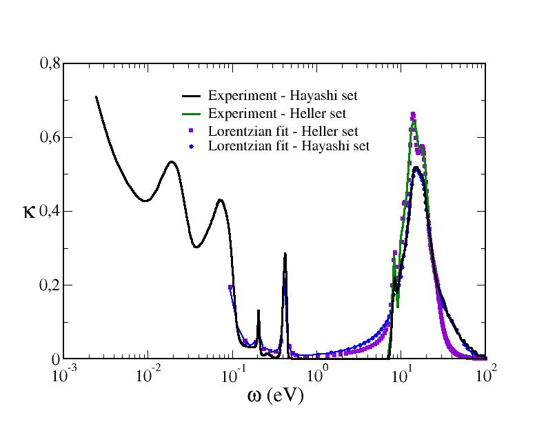
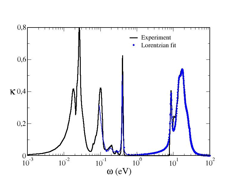
Figure 9: Experimental data of extinction index ($\kappa$), and parametric representations with Lorentzian oscillators. Experimental results for water (top), displaying the Hayashi and Heller sets together with parametrizations using the Lorentz model from this work. Experimental results for ice (bottom), compared to fit with Lorentz model. Symbols correspond (roughly) to extinction indexes measured at Matsubara frequencies (some of the highly dense frequencies were removed for clarity of presentation).

For water the high energy band is very accurately reproduced in the important region above ca. 10 eV, both for the Hayashi and Heller sets. The less important IR region is reproduced only qualitatively. For ice, the high energy band is also well reproduced, except for a small shoulder occurring at about 10 eV, which could not be reproduced by the model without spoiling the rest of the fit. The IR region in this case is more faithfully reproduced than it is for water. Together with our fits, Fig.1-top of the main manuscript also displays the extinction coefficients of liquid water and ice predicted by the model of ES,[28] which appears to differ significantly from our fit to the Heller data set.

A.4 Quantum density functional theory calculations

Since there appears to be some degree of uncertainty as regards the experimental measurement of Dielectric functions, we have also performed quantum density functional theory calculations (DFT). Results obtained in this way are only approximate, but the calculations are performed under the same footing for both water and ice. This is not the case for experimental studies, because it takes some approximations to resolve the signal from the instrumental resolution, and absorption of vapor from the liquid surface hampers the data analysis.[45]

In order to simplify the calculations, we first performed classical simulations of bulk ice and water at T=273 K using the TIP4P/Ice model.[70] Because of the computational cost, simulations were performed for samples of 16 molecules under periodic boundary conditions and the minimum image convention. After equilibration, we performed a batch of 12 consecutive runs, and stored the final configuration of each run for further analysis. In the case of ice, each of the 12 configurations was obtained from an independent hydrogen bond arrangement sampled according to the ice rules.[139, 140] In practice, we find the high energy band displays a very small dependence of the selected configuration, in line with other studies.[141] The thermalized configurations are used as input for the DFT calculations, which are used to relax the intramolecular degrees of freedom of the H₂O molecules.

The Electronic structure calculations are performed using the Perdew-Burke-Ernzerhof (PBE) functional,[55] which, as other generalized gradient functionals is widely used to study energetic properties of ice and water.[142, 143, 144, 145] PBE does not account properly for dispersion interactions, which are known to have an important impact in water thermodynamic properties.[146, 147, 148] However, here the configuration space of the nuclei is sampled from an empirical potential anyway, and we do not expect large corrections to the electronic properties from dispersion effects.[145]

To solve the Kohn-Sham equations, we employ the Vienna Ab innitio Simulation Package (VASP),[52, 53, 54] using a plane wave basis set with cutoff at 700 eV for the valence electrons, and core electrons treated with pseudopotentials in the projected augmented wave approximation (PAW).[149, 150]

In order to obtain the optical properties in the high energy region, results from the PBE calculations are post processed under the GW/RPA approximation,[56, 57, 141]. For further details, the reader is referred to references [58, 59]. Optical properties in the vibrational region are obtained using Density Functional Perturbation Theory [151].

Figure 10 displays the absorption spectrum obtained from the DFT calculations for both ice and water. Whereas it is clear that a quantitative agreement with experiment is not achieved, the PBE functional provides a reasonable qualitative description of the absorption spectrum. Particularly, the calculations yield a first electronic excitation in the range of decades of eV–admittedly, with significantly smaller intensity–followed by a strong adsorption close to 20 eV. In the IR region, DFT calculations from frozen configuration only provide the absorption frequencies, and the spectrum shows results obtained with an assumed constant band width of 0.02 eV for the sake of illustration. Bearing this in mind, we find that the density of normal modes is well reproduced and displays significantly sharper features for ice than for water, as observed in experiments. Since no dynamics is input into the calculations, we are unable to reproduce the MW region of liquid water, but this fortunately is inconsequential as far as the calculation of Hamaker functions is concerned.

For the purpose of calculating the Hamaker function, we obtain the dielectric function at imaginary frequencies by using the Kramers-Kronig relation of Eq. (31). In order to ease the calculations, the resulting function is fitted to a model of Drude oscillators, Eq. (33), with zero band width (i.e. $B_{i}=0$). The parameters obtained from the fit may be found in Table 7.

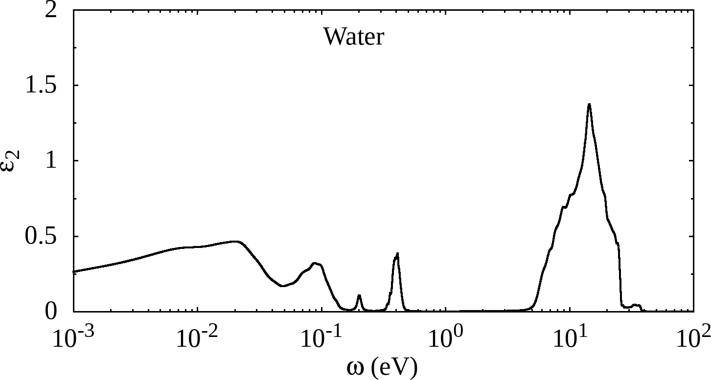
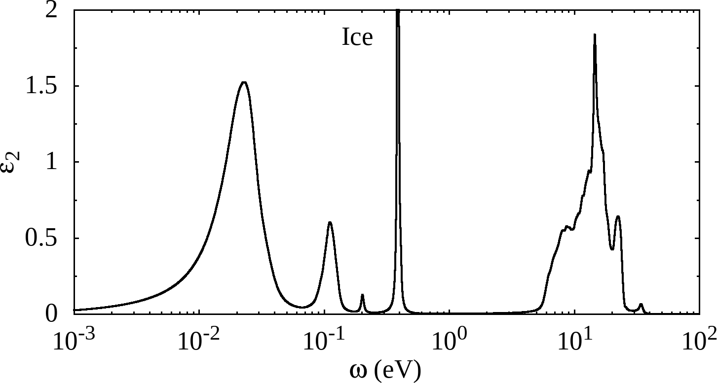
Figure 10: Real and imaginary parts of the complex dielectric function as obtained from DFT calculations. Compared to liquid water, the absorption bands appear sharper for ice due to its ordered structure.

Appendix B Parameters set

$A_{k}$	$B_{k}\cdot$eV	$C_{k}\cdot$eV2
4.69	610.70	2587.34
2.21	83.09	2119.77
0.50	8.13	186.75
1.97x$10^{-2}$	0.40	24.25
7.51x$10^{-3}$	0.94	14.57
5.79x$10^{-2}$	0.22	5.74
1.13x$10^{-2}$	5.22x$10^{-3}$	1.44x$10^{-2}$
0.57	3.88x$10^{-2}$	5.02x$10^{-3}$
0.17	2.22x$10^{-2}$	2.96x$10^{-3}$
8.28x$10^{-2}$	2.04x$10^{-2}$	1.59x$10^{-3}$
0.11	1.91x$10^{-2}$	6.05x$10^{-4}$

Table 4: Parameters set for Liquid Water - Hayashi. The CSF is applied to the eighth oscillator, with $\omega_{0}=7.7\ eV$ and $\Delta\omega=0.1\ eV^{4}$

$A_{k}$	$B_{k}\cdot$eV	$C_{k}\cdot$eV2
4.69	610.70	2587.34
2.21	83.09	2119.77
0.50	8.13	186.75
1.97x$10^{-2}$	0.40	24.25
7.51x$10^{-3}$	0.94	14.57
5.79x$10^{-2}$	0.22	5.74
8.02x$10^{-2}$	1.70x$10^{-2}$	1.46x$10^{-2}$
8.99x$10^{-2}$	1.38x$10^{-2}$	8.73x$10^{-3}$
0.37	2.06x$10^{-2}$	5.58x$10^{-3}$
0.31	2.04x$10^{-2}$	3.21x$10^{-3}$
0.10	1.71x$10^{-2}$	1.56x$10^{-3}$

Table 5: Parameters set for Liquid Water - Heller. The CSF is applied to the seventh to tenth oscillators, with $\omega_{0}=7.7\ eV$ and $\Delta\omega=500.0\ eV^{4}$

$A_{k}$	$B_{k}\cdot$eV	$C_{k}\cdot$eV2
0.40	26.22	3328.19
0.30	7.66	1545.24
0.25	2.72	105.58
2.44x$10^{-2}$	1.10	25.88
1.03x$10^{-2}$	0.62	12.99
8.66x$10^{-2}$	0.16	6.24
9.39x$10^{-2}$	1.23x$10^{-2}$	1.35x$10^{-2}$
0.28	2.26x$10^{-2}$	5.03x$10^{-3}$
0.24	1.76x$10^{-2}$	3.25x$10^{-3}$
0.12	1.66x$10^{-2}$	1.73x$10^{-3}$
1.47x$10^{-3}$	1.37x$10^{-3}$	1.29x$10^{-3}$

Table 6: Parameters set for Ice. The CSF is applied to the seventh to ninth oscillators, with $\omega_{0}=8.1\ eV$ and $\Delta\omega=0.1\ eV^{4}$

Water		Ice
$A_{k}$	$C_{k}\cdot$eV2	$A_{k}$	$C_{k}\cdot$eV2
0.646	1.21x$10^{+8}$	0.198	1.23x$10^{+8}$
0.281	4.90x$10^{+6}$	0.154	6.08x$10^{+3}$
0.582	5.91x$10^{+4}$	0.836	1.79x$10^{+3}$
0.534	2.84x$10^{+3}$	0.132	8.28x$10^{+1}$
0.184	6.89x$10^{+1}$	0.126	6.11
0.180	2.83x$10^{-2}$	0.279	1.36x$10^{-2}$
0.539	3.87x$10^{-3}$	0.362	3.13x$10^{-3}$

Table 7: Parameters sets for liquid water and ice from fitting DFT calculations to 7 Lorentz oscillators without width.

References

- Björneholm et al. [2016] O. Björneholm, M. H. Hansen, A. Hodgson, L.-M. Liu, D. T. Limmer, A. Michaelides, P. Pedevilla, J. Rossmeisl, H. Shen, G. Tocci, E. Tyrode, M.-M. Walz, J. Werner, and H. Bluhm, Water at interfaces, Chem. Rev. 116, 7698 (2016), pMID: 27232062, https://doi.org/10.1021/acs.chemrev.6b00045 .
- Bartels-Rausch et al. [2012] T. Bartels-Rausch, V. Bergeron, J. H. E. Cartwright, R. Escribano, J. L. Finney, H. Grothe, P. J. Gutiérrez, J. Haapala, W. F. Kuhs, J. B. C. Pettersson, S. D. Price, C. I. Sainz-Díaz, D. J. Stokes, G. Strazzulla, E. S. Thomson, H. Trinks, and N. Uras-Aytemiz, Ice structures, patterns, and processes: A view across the icefields, Rev. Mod. Phys. 84, 885 (2012).
- Libbrecht [2022] K. G. Libbrecht, Snow Crystals (Princeton University Press, 2022).
- Pruppacher and Klett [2010] H. R. Pruppacher and J. D. Klett, Microphysics of Clouds and Precipitation (Springer, Heidelberg, 2010).
- Weyl [1951] W. Weyl, Surface structure of water and some of its physical and chemical manifestations, J. Colloid. Sci. 6, 389 (1951).
- Lipowsky [1982] R. Lipowsky, Critical surface phenomena at first-order bulk transitions, Phys. Rev. Lett. 49, 1575 (1982).
- Dietrich [1988] S. Dietrich, Wetting phenomena, in Phase Transitions and Critical Phenomena, Vol. 12, edited by C. Domb and J. L. Lebowitz (Academic, New York, 1988) pp. 1–89.
- Schick [1990] M. Schick, Introduction to wetting phenomena, in Liquids at Interfaces, Les Houches Lecture Notes (Elsevier, Amsterdam, 1990) pp. 1–89.
- Jellinek [1967] H. Jellinek, Liquid-like (transition) layer on ice, J. Colloid. Interface Sci. 25, 192 (1967).
- Nenow [1984] D. Nenow, Surface premelting, Prog. Cryst. Growth Charact. Mater. 9, 185 (1984).
- Petrenko [1994] V. F. Petrenko, The Surface of Ice, Cold Regions Research and Engineering Laboratory (Special Report 94-22) (1994).
- Dash et al. [1995] J. G. Dash, H. Fu, and J. S. Wettlaufer, The premelting of ice and its environmental consequences, Reports on Progress in Physics 58, 115 (1995).
- Rosenberg [2005] R. Rosenberg, Why is ice slippery?, Phys. Today 58, 50 (2005).
- Dash et al. [2006] J. G. Dash, A. W. Rempel, and J. S. Wettlaufer, The physics of premelted ice and its geophysical consequences, Rev. Mod. Phys. 78, 695 (2006).
- Slater and Michaelides [2019] B. Slater and A. Michaelides, Surface premelting of water ice, Nat. Rev. Chem 3, 172 (2019).
- Nagata et al. [2019] Y. Nagata, T. Hama, E. H. G. Backus, M. Mezger, D. Bonn, M. Bonn, and G. Sazaki, The surface of ice under equilibrium and nonequilibrium conditions, Acc. Chem. Res. 52, 1006 (2019).
- Elbaum [1991] M. Elbaum, Roughening transition observed on the prism facet of ice, Phys. Rev. Lett. 67, 2982 (1991).
- Wettlaufer [1999] J. Wettlaufer, Impurity effects in the premelting of ice, Phys. Rev. Lett. 82, 2516 (1999).
- Li and Somorjai [2007] Y. Li and G. A. Somorjai, Surface premelting of ice, J. Phys. Chem. C 111, 9631 (2007).
- Llombart et al. [2020a] P. Llombart, E. G. Noya, D. N. Sibley, A. J. Archer, and L. G. MacDowell, Rounded layering transitions on the surface of ice, Phys. Rev. Lett. 124, 065702 (2020a).
- Sibley et al. [2021] D. Sibley, P. Llombart, E. G. Noya, A. Archer, and L. G. MacDowell, How ice grows from premelting films and liquid droplets, Nat. Commun. 12, 239 (2021).
- Lipowsky et al. [1989] R. Lipowsky, U. Breuer, K. C. Prince, and H. P. Bonzel, Multicomponent order parameter for surface melting, Phys. Rev. Lett. 62, 913 (1989).
- Limmer and Chandler [2014] D. T. Limmer and D. Chandler, Premelting, fluctuations, and coarse-graining of water-ice interfaces, J. Chem. Phys. 141, 18C505 (2014).
- Li et al. [2019] H. Li, M. Bier, J. Mars, H. Weiss, A.-C. Dippel, O. Gutowski, V. Honkimäki, and M. Mezger, Interfacial premelting of ice in nano composite materials, Phys. Chem. Chem. Phys. 21, 3734 (2019).
- Chernov and Mikheev [1988] A. A. Chernov and L. V. Mikheev, Wetting of solid surfaces by a structured simple liquid: Effect of fluctuations, Phys. Rev. Lett. 60, 2488 (1988).
- Henderson [1994] J. R. Henderson, Wetting phenomena and the decay of correlations at fluid interfaces, Phys. Rev. E 50, 4836 (1994).
- Henderson [2005] J. R. Henderson, Statistical mechanics of the disjoining pressure of a planar film, Phys. Rev. E 72, 051602 (2005).
- Elbaum and Schick [1991a] M. Elbaum and M. Schick, Application of the theory of dispersion forces to the surface melting of ice, Phys. Rev. Lett. 66, 1713 (1991a).
- Parsegian [2005] V. A. Parsegian, Van der Waals Forces (Cambridge University Press, Cambridge, 2005) pp. 1–311.
- Parsegian and Weiss [1981] V. A. Parsegian and G. H. Weiss, Spectroscopic parameters for computation of van der waals forces, J. Colloid. Interface Sci. 81, 285 (1981).
- Roth and Lenhoff [1996] C. M. Roth and A. M. Lenhoff, Improved parametric representation of water dielectric data for lifshit z theory calculations, J. Colloid. Interface Sci. 179, 637 (1996).
- Dagastine et al. [2000] R. R. Dagastine, D. C. Prieve, and L. R. White, The dielectric function for water and its application to van der waals forces, J. Colloid. Interface Sci. 231, 351 (2000).
- Fernández-Varea and Garcia-Molina [2000] J. M. Fernández-Varea and R. Garcia-Molina, Hamaker constants of systems involving water obtained from a dielectric function that fulfills the f sum rule, J. Colloid. Interface Sci. 231, 394 (2000).
- Wang and Nguyen [2017] J. Wang and A. V. Nguyen, A review on data and predictions of water dielectric spectra for calcul ations of van der waals surface forces, Adv. Colloid Interface Sci. 250, 54 (2017).
- Luengo [2019] J. Luengo, Fuerzas de van der waals en la superficie del hielo, Degree Thesis (2019), universidad Complutense de Madrid.
- Luengo and MacDowell [2020] J. Luengo and L. MacDowell, Van der Waals Forces at Ice Surfaces with Atmospheric Interest, Master’s thesis, Facultad de Ciencias (2020).
- Fiedler et al. [2020] J. Fiedler, M. Boström, C. Persson, I. Brevik, R. Corkery, S. Y. Buhmann, and D. F. Parsons, Full-spectrum high-resolution modeling of the dielectric function of water, J. Phys. Chem. B 124, 3103 (2020), pMID: 32208624, https://doi.org/10.1021/acs.jpcb.0c00410 .
- Luengo-Márquez and MacDowell [2021] J. Luengo-Márquez and L. G. MacDowell, Lifshitz theory of wetting films at three phase coexistence: The case of ice nucleation on silver iodide (agi), Journal of Colloid and Interface Science 590, 527 (2021).