Investigating the $\mathbf{\Upsilon(10753)\to\Upsilon(1^{3}D_{J})\eta}$ transitions

Abstract

In this work, we investigate the $\Upsilon(10753)\to\Upsilon(1^{3}D_{J})\eta$ ($J=1,2,3$) processes, where the $\Upsilon(10753)$ is assigned as a conventional bottomonium under the $4S$-$3D$ mixing scheme. Our result shows that the concerned processes have considerable branching ratios, i.e., branching ratios $\mathcal{B}[\Upsilon(10753)\to\Upsilon(1^{3}D_{1})\eta]$ and $\mathcal{B}[\Upsilon(10753)\to\Upsilon(1^{3}D_{2})\eta]$ can reach up to the order of magnitude of $10^{-4}-10^{-3}$, while $\mathcal{B}[\Upsilon(10753)\to\Upsilon(1^{3}D_{3})\eta]$ is around $10^{-6}-10^{-5}$. With the running of Belle II, it is a good opportunity for finding out the concerned hidden-bottom hadronic decays.

I introduction

As presented in the Belle II physics book Belle-II:2018jsg , the designed luminosity of SuperKEKB can reach up to $8\times 10^{35}\text{cm}^{-2}\text{s}^{-1}$. Thus, the forthcoming Belle II experiment represents the precision frontier of particle physics, which is an ideal platform to perform the correlative study around heavy flavor physics. Obviously, some higher bottomonia can be accessible at Belle II, which may provide valuable hints to construct the bottomonium family.

Recently, the $\Upsilon(10753)$ was reported by the Belle Collaboration by analyzing the $e^{+}e^{-}\to\Upsilon(nS)\pi^{+}\pi^{-}$ ($n=1,2,3$) processes Belle:2019cbt . As a vector state, the $\Upsilon(10753)$ was also collected in Particle Data Group (PDG) ParticleDataGroup:2020ssz . Since a peculiar property of the $\Upsilon(10753)$ is its mass lower than the predicted mass of the $\Upsilon(3^{3}D_{1})$ by the quenched potential model Godfrey:2015dia ; Segovia:2016xqb ; Wang:2018rjg , thus different theoretical groups tried to explain the observed $\Upsilon(10753)$ as exotic states like the tetraquark state Wang:2019veq ; Ali:2020svd , the hybrid state TarrusCastella:2021pld , and the kinetic effect Bicudo:2019ymo ; Bicudo:2020qhp .

Inspired by the $2S$-$1D$ mixing scheme for the charmonium $\psi(3770)$, we have a reason to believe that the $S$-$D$ mixing scheme should be considered when revealing the nature of the $\Upsilon(10753)$. Thus, the Lanzhou group introduced the $4S$-$3D$ mixing scheme to clarify the puzzling phenomenon of the $\Upsilon(10753)$ Li:2021jjt ; Bai:2022cfz . In Ref. Li:2021jjt , the Lanzhou group proposed the $4S$-$3D$ mixing scheme, which can solve the mass puzzle of the $\Upsilon(10753)$. A later result in Ref. Bai:2022cfz shows that the $\Upsilon(10753)$ under this mixing scheme has sizable dielectron decay width and the measured values $\mathcal{R}_{n}=\Gamma_{e^{+}e^{-}}\times\mathcal{B}[\Upsilon(10753)\to\Upsilon(nS)\pi^{+}\pi^{-}]$ ($n=1,2,3$) by Belle Belle:2019cbt can be reproduced. In summary, the current measured data of the $\Upsilon(10753)$ Belle:2019cbt , including its mass and $\mathcal{R}_{n}$ values, can well be understood under the $4S$-$3D$ mixing scheme. Thus, the $\Upsilon(10753)$ can be still a good candidate of vector bottomonium. Along this line, several typical transitions of the $\Upsilon(10753)$ into other bottomonia with lower mass were explored in Refs. Li:2021jjt ; Bai:2022cfz , which will be accessible at a future experiment like Belle II. In Fig. 1, we summarize the present status of the study of the transitions of the $\Upsilon(10753)$ into other bottomonia.

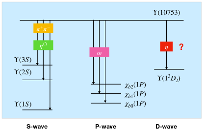
Figure 1: The present status of the study on the transitions of the $\Upsilon(10753)$ into other bottomonia.

Obviously, our knowledge of the transitions of the $\Upsilon(10753)$ into other bottomonia is still absent. A typical example is that the allowed $\Upsilon(10753)\to\Upsilon(1^{3}D_{2})\eta$ is waiting to be explored, not only by theorists but also by experimentalists. This fact stimulates our interest in carrying out the investigation of $\Upsilon(10753)\to\Upsilon(1^{3}D_{J})\eta$ ($J=1,2,3$), where the $\Upsilon(1^{3}D_{J})$ denote three $1D$ bottomonium states. By checking the PDG values ParticleDataGroup:2020ssz , we may find that only $\Upsilon(1^{3}D_{2})$ was observed. For the remaining $1D$ bottomonia, they are still missing in experiment. Thus, the present study of $\Upsilon(10753)\to\Upsilon(1^{3}D_{J})\eta$ has a close relation to these two missing bottomonia $\Upsilon(1^{3}D_{1})$ and $\Upsilon(1^{3}D_{3})$.

For calculating the branching ratio of the $\Upsilon(10753)\to\Upsilon(1^{3}D_{J})\eta$ transitions, the concrete phenomenological model should be involved. Borrowing the former experience of the decays of higher states of heavy quarkonium, the coupled channel effect should be considered here Meng:2007tk ; Meng:2008dd ; Meng:2008bq ; Chen:2011jp ; Chen:2011qx ; Chen:2011zv ; Chen:2014ccr ; Wang:2016qmz ; Huang:2017kkg ; Zhang:2018eeo ; Huang:2018pmk ; Huang:2018cco ; Li:2021jjt ; Bai:2022cfz . In this work, we adopt the hadronic loop mechanism to present the concrete calculation, which will be mentioned in the following section. We hope that our realistic investigation of the discussed processes may provide valuable information to experimentally search for $\Upsilon(10753)\to\Upsilon(1^{3}D_{J})\eta$, which will be an intriguing research task for Belle II.

This paper is organized as follows. After the introduction, we illustrate the detailed calculation of $\Upsilon(10753)\to\Upsilon(1^{3}D_{J})\eta$ ($J=1,2,3$) with the hadronic loop mechanism in Sec. II. And then, the numerical results are presented in Sec. III. Finally, we end the paper with a discussion and conclusion.

II the $\mathbf{\Upsilon(10753)\to\Upsilon(1^{3}D_{J})\eta}$ transitions via the hadronic loop mechanism

Before studying the decays, we need to briefly introduce the $4S$-$3D$ mixing scheme. If assigning the $\Upsilon(10753)$ as the pure $\Upsilon(3D)$ state, the predicted mass of pure $\Upsilon(3D)$ state ranges from $10653$ MeV to $10717$ MeV Badalian:2008ik ; Badalian:2009bu ; Godfrey:2015dia ; Segovia:2016xqb ; Wang:2018rjg . Thus, there exists difference between the theoretical result and current measurement of the $\Upsilon(10753)$. Furthermore, the dielectron width of the $\Upsilon(3D)$ was estimated to be just a few eV Godfrey:2015dia ; Wang:2018rjg ; Badalian:2008ik ; Badalian:2009bu , which is lower than the corresponding dielectron widths of the $\Upsilon(4S)$ and $\Upsilon(5S)$ states. Thus, it is difficult to find pure $\Upsilon(3D)$ state via the electron-positron annihilation process. However, the $\Upsilon(10753)$ signal was observed in the $e^{+}e^{-}\to\Upsilon(nS)\pi^{+}\pi^{-}$ processes by Belle Belle:2019cbt , which is puzzling for us. As proposed in Refs. Li:2021jjt ; Bai:2022cfz , the $4S$-$3D$ mixing scheme for the $\Upsilon(10753)$ was introduced

$$\left(\begin{array}[]{c}\Upsilon_{4S-3D}\\ \Upsilon^{\prime}_{4S-3D}\end{array}\right)=\left(\begin{array}[]{cc}\cos{\theta}&-\sin{\theta}\\ \sin{\theta}&\cos{\theta}\end{array}\right)\left(\begin{array}[]{c}\Upsilon({4S})\\ \Upsilon({3D})\end{array}\right),$$ (2.1)

where $\theta$ denotes the mixing angle, and $\Upsilon_{{4S-3D}}$ and $\Upsilon_{{4S-3D}}^{\prime}$ are physical states. Here, the $\Upsilon_{{4S-3D}}^{\prime}$ state corresponds to the observed $\Upsilon(10753)$. Obviously, the puzzle on mass can be solved as shown in Fig. 1 of Ref. Li:2021jjt , and the dielectron decay width of the $\Upsilon(10753)$ is sizable. Thus, the $\Upsilon(10753)$ still can be as a good candidate of vector bottomonium.

Based on hadronic loop mechanism, the initial $\Upsilon(10753)$ can be converted into final low-lying $D$-wave bottomonium $\Upsilon(1^{3}D_{J})$ through the triangle loops composed of bottom mesons. The concerned diagrams are displayed in Fig. 2, where the contributions from the $B_{s}^{(*)}$ meson loops can be ignored due to the weak coupling between the $\Upsilon(10753)$ and the $B_{s}^{(*)}\bar{B}_{s}^{(*)}$ pair Liang:2019geg .

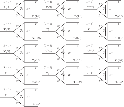
Figure 2: The schematic diagrams for depicting the $\Upsilon(4S,3D)\to\Upsilon(1^{3}D_{J})\eta$ decays via the hadronic loop mechanism, where $\Upsilon^{\prime}$ and $\Upsilon_{1}^{\prime}$ represent the $\Upsilon(4S)$ and $\Upsilon(3D)$ components of the $\Upsilon(10753)$, respectively.

For the diagrams shown in Fig. 2, the general expression of their amplitude mediated by the hadronic loop mechanism reads as

$$\mathcal{M}=\int\frac{d^{4}q}{(2\pi)^{4}}\frac{\mathcal{V}_{1}\mathcal{V}_{2}\mathcal{V}_{3}}{\mathcal{P}_{1}\mathcal{P}_{2}\mathcal{P}_{E}}\mathcal{F}^{2}(q^{2},m_{E}^{2}),$$ (2.2)

where $\mathcal{V}_{\text{i}}$ ($i=1,2,3$) are interaction vertices, and $1/\mathcal{P}_{1,2,E}$ denote the corresponding propagators of intermediate bottom mesons. In addition, the form factor $\mathcal{F}(q^{2},m_{E}^{2})$ should be introduced to compensate the off shell effect of the exchanged $B^{(*)}$ meson and depict the structure effect of interaction vertices Locher:1993cc ; Li:1996yn ; Cheng:2004ru . In our calculation, the monopole form factor Gortchakov:1995im

$$\mathcal{F}(q^{2},m_{E}^{2})=\frac{\Lambda^{2}-m_{E}^{2}}{\Lambda^{2}-q^{2}}\quad{\text{w}ith}\quad\Lambda=m_{E}+\alpha_{\Lambda}\Lambda_{QCD}$$ (2.3)

emphasized by QCD sum rules is adopted with $m_{E}$ and $q$ denoting the mass and four-momentum of the exchanged intermediate meson, respectively. Here, we take $\Lambda_{QCD}=220$ MeV Liu:2006dq ; Liu:2009dr ; Li:2013zcr , and $\alpha_{\Lambda}$ is a phenomenological dimensionless parameter.

The effective Lagrangian approach is used to give the concrete expressions of the decay amplitudes defined in Eq. (2.2). Due to the requirement from the heavy quark limit and the chiral symmetry, the concerned effective Lagrangians include Casalbuoni:1996pg ; Wise:1992hn ; Xu:2016kbn ; Duan:2021bna

$$\begin{split}\mathcal{L}_{S}=&\ ig_{S}\text{Tr}[S^{(b\bar{b})}\bar{H}^{(\bar{b}q)}\gamma^{\mu}\overset{\leftrightarrow}{\partial}_{\mu}\bar{H}^{(b\bar{q})}]+\text{H.c.},\\ \mathcal{L}_{D}=&\ ig_{D}\text{Tr}[D_{\mu\nu}^{(b\bar{b})}\bar{H}^{(\bar{b}q)}\overset{\leftrightarrow}{\partial}_{\mu}\gamma^{\nu}\bar{H}^{(b\bar{q})}]+\text{H.c.},\\ \mathcal{L}_{\mathbb{P}}=&\ ig_{H}\text{Tr}[H^{(b\bar{q})\text{j}}\gamma_{\mu}\gamma_{5}(\mathcal{A}^{\mu})^{\text{i}}_{\text{j}}\bar{H}_{\text{i}}^{(b\bar{q})}]\end{split}$$ (2.4)

with $\overset{\leftrightarrow}{\partial}\equiv\overset{\rightarrow}{\partial}-\overset{\leftarrow}{\partial}$. Here, the abbreviations $S^{(b\bar{b})}$ and $D_{\mu\nu}^{(b\bar{b})}$ represent the $S$-wave and $D$-wave multiplets of bottomonium, respectively, i.e.,

$$S^{(b\bar{b})}=\frac{1+\not{\upsilon}}{2}\left[\Upsilon^{\mu}\gamma_{\mu}-\eta_{b}\gamma_{5}\right]\frac{1-\not{\upsilon}}{2},$$ (2.5)

$$\begin{split}D^{(b\bar{b})\mu\nu}=&\frac{1+\not{\upsilon}}{2}\left[\Upsilon_{3}^{\mu\nu\alpha}\gamma_{\alpha}+\frac{1}{\sqrt{6}}\left(\varepsilon^{\mu\alpha\beta\rho}\upsilon_{\alpha}\gamma_{\beta}\Upsilon_{2\rho}^{\nu}+\varepsilon^{\nu\alpha\beta\rho}\upsilon_{\alpha}\gamma_{\beta}\right.\right.\\ &\left.\left.\times\Upsilon_{2\rho}^{\mu}\right)+\frac{\sqrt{15}}{10}\left[\left(\gamma^{\mu}-\upsilon^{\mu}\right)\Upsilon_{1}^{\nu}+\left(\gamma^{\nu}-\upsilon^{\nu}\right)\Upsilon_{1}^{\mu}\right]\right.\\ &\left.-\frac{1}{\sqrt{15}}\left(g^{\mu\nu}-\upsilon^{\mu}\upsilon^{\nu}\right)\gamma_{\alpha}\Upsilon_{1}^{\alpha}+\eta_{b2}^{\mu\nu}\gamma_{5}\right]\frac{1-\not{\upsilon}}{2}.\end{split}$$ (2.6)

Additionally, the $(0^{-},1^{-})$ doublets of bottom and antibottom mesons is abbreviated as $H^{(b\bar{q})}$ and $H^{(\bar{b}q)}$, respectively, which can be expressed as

$$\begin{split}H^{(b\bar{q})}=&\frac{1+\not{\upsilon}}{2}\left(\mathcal{B}^{*\mu}\gamma_{\mu}+i\mathcal{B}\gamma_{5}\right),\\ H^{(\bar{b}q)}=&\left(\bar{\mathcal{B}}^{*\mu}\gamma_{\mu}+i\bar{\mathcal{B}}\gamma_{5}\right)\frac{1-\not{\upsilon}}{2},\end{split}$$ (2.7)

where the normalization factor $\sqrt{m_{\mathcal{B}^{(*)}}}$ is neglected here. The $\bar{H}^{(b\bar{q})}$ and $\bar{H}^{(\bar{b}q)}$ fields can be obtained through $\bar{H}^{(b\bar{q})}=\gamma_{0}H^{\dagger(b\bar{q})}\gamma_{0}$ and $\bar{H}^{(\bar{b}q)}=\gamma_{0}H^{\dagger(\bar{b}q)}\gamma_{0}$. $\mathcal{A^{\mu}}$, the axial vector current of Nambu-Goldstone fields, is expressed as $\mathcal{A}^{\mu}=(\xi^{\dagger}\partial^{\mu}\xi-\xi\partial^{\mu}\xi^{\dagger})/2$ with $\xi=e^{i\mathbb{P}/f_{\pi}}$, where the pseudoscalar octet $\mathbb{P}$ is

$$\begin{split}\mathbb{P}&=\begin{pmatrix}-\frac{\pi^{0}}{\sqrt{2}}+\frac{\eta_{8}}{\sqrt{6}}&\pi^{+}&K^{+}\\ -\pi^{-}&\frac{\pi^{0}}{\sqrt{2}}+\frac{\eta_{8}}{\sqrt{6}}&K^{0}\\ -K^{-}&\bar{K}^{0}&-\frac{2}{\sqrt{6}}\eta_{8}\end{pmatrix}.\\ \end{split}$$ (2.8)

With the above preparation, we expand the compact Lagrangians in Eq. (2.4) to get the following effective Lagrangians

$$\begin{split}\mathcal{L}_{\Upsilon\mathcal{B}^{(*)}\mathcal{B}^{(*)}}=&\ ig_{\Upsilon\mathcal{B}\mathcal{B}}\Upsilon^{\mu}(\partial_{\mu}\mathcal{B}^{\dagger}\mathcal{B}-\mathcal{B}^{\dagger}\partial_{\mu}\mathcal{B})\\ &+g_{\Upsilon\mathcal{B}\mathcal{B}^{*}}\varepsilon_{\mu\nu\alpha\beta}\partial^{\mu}\Upsilon^{\nu}(\mathcal{B}^{*\alpha\dagger}\overset{\leftrightarrow}{\partial^{\beta}}\mathcal{B}-\mathcal{B}^{\dagger}\overset{\leftrightarrow}{\partial^{\beta}}\mathcal{B}^{*\alpha})\\ &+ig_{\Upsilon\mathcal{B}^{*}\mathcal{B}^{*}}\Upsilon^{\mu}(\partial_{\nu}\mathcal{B}_{\mu}^{*\dagger}\mathcal{B}^{*\nu}-\mathcal{B}^{*\nu\dagger}\partial_{\nu}\mathcal{B}_{\mu}^{*}+\mathcal{B}^{*\nu\dagger}\overset{\leftrightarrow}{\partial}_{\mu}\mathcal{B}_{\nu}^{*}),\end{split}$$ (2.9)

$$\begin{split}\mathcal{L}_{\Upsilon_{1}\mathcal{B}^{(*)}\mathcal{B}^{(*)}}=&\ ig_{\Upsilon_{1}\mathcal{B}\mathcal{B}}\Upsilon_{1}^{\mu}(\partial_{\mu}\mathcal{B}^{\dagger}\mathcal{B}-\mathcal{B}^{\dagger}\partial_{\mu}\mathcal{B})\\ &{+g_{\Upsilon_{1}\mathcal{B}\mathcal{B}^{*}}\varepsilon_{\mu\nu\alpha\beta}\partial^{\mu}\Upsilon_{1}^{\nu}(\mathcal{B}^{*\alpha\dagger}\overset{\leftrightarrow}{\partial^{\beta}}\mathcal{B}-\mathcal{B}^{\dagger}\overset{\leftrightarrow}{\partial^{\beta}}\mathcal{B}^{*\alpha})}\\ &+ig_{\Upsilon_{1}\mathcal{B}^{*}\mathcal{B}^{*}}\Upsilon_{1}^{\mu}(\partial_{\nu}\mathcal{B}_{\mu}^{*\dagger}\mathcal{B}^{*\nu}-\mathcal{B}^{*\nu\dagger}\partial_{\nu}\mathcal{B}_{\mu}^{*}\\ &+4\mathcal{B}^{*\nu\dagger}\overset{\leftrightarrow}{\partial}_{\mu}\mathcal{B}_{\nu}^{*}),\end{split}$$ (2.10)

$$\begin{split}\mathcal{L}_{\Upsilon_{2}\mathcal{B}^{(*)}\mathcal{B}^{*}}=&-ig_{\Upsilon_{2}\mathcal{B}\mathcal{B}^{*}}\Upsilon_{2}^{\mu\nu}(\mathcal{B}^{\dagger}\overset{\leftrightarrow}{\partial_{\mu}}\mathcal{B}^{*}_{\nu}-\mathcal{B}^{*\dagger}_{\nu}\overset{\leftrightarrow}{\partial_{\mu}}\mathcal{B})\\ &+g_{\Upsilon_{2}\mathcal{B}^{*}\mathcal{B}^{*}}\varepsilon_{\mu\nu\alpha\beta}\partial^{\nu}\Upsilon_{2}^{\rho\beta}(\mathcal{B}^{*\dagger}_{\rho}\overset{\leftrightarrow}{\partial^{\mu}}\mathcal{B}^{*\alpha}+\mathcal{B}^{*\alpha\dagger}\overset{\leftrightarrow}{\partial^{\mu}}\mathcal{B}^{*}_{\rho}),\end{split}$$ (2.11)

$$\mathcal{L}_{\Upsilon_{3}\mathcal{B}^{*}\mathcal{B}^{*}}=-ig_{\Upsilon_{3}\mathcal{B}^{*}\mathcal{B}^{*}}\Upsilon_{3}^{\mu\nu\alpha}(\mathcal{B}^{*\dagger}_{\nu}\overset{\leftrightarrow}{\partial_{\mu}}\mathcal{B}^{*}_{\alpha}+\mathcal{B}^{*\dagger}_{\alpha}\overset{\leftrightarrow}{\partial_{\mu}}\mathcal{B}^{*}_{\nu}),$$ (2.12)

$$\begin{split}\mathcal{L}_{\mathcal{B}^{(*)}\mathcal{B}^{*}\mathbb{P}}=&\ ig_{\mathcal{B}\mathcal{B}^{*}\mathbb{P}}(\mathcal{B}_{\mu}^{*\dagger}\mathcal{B}-\mathcal{B}^{\dagger}\mathcal{B}_{\mu}^{*})\partial^{\mu}\mathbb{P}\\ &-g_{\mathcal{B}^{*}\mathcal{B}^{*}\mathbb{P}}\varepsilon_{\mu\nu\alpha\beta}\partial^{\mu}\mathcal{B}^{*\dagger\nu}\partial^{\alpha}\mathcal{B}^{*\beta}\mathbb{P},\end{split}$$ (2.13)

where $\mathcal{B}^{(*)\dagger}$ and $\mathcal{B}^{(*)}$ are defined as $\mathcal{B}^{(*)\dagger}=(B^{(*)+},B^{(*)0},B_{s}^{(*)0})$ and $\mathcal{B}^{(*)}=(B^{(*)-},\bar{B}^{(*)0},\bar{B}_{s}^{(*)0})^{T}$, respectively.

Now, we can write down the concrete amplitudes according to the diagrams in Fig. 2 by the Feynman rules listed in Appendix A. With the first diagram in Fig. 2 as an example, the expression of its amplitude is

$$\begin{split}\mathcal{M}_{4S}^{(1-1)}=&\frac{|\vec{p}_{\eta}|}{32\pi^{2}m}\int d\Omega\ \epsilon_{\Upsilon^{\prime}}^{\mu}g_{\Upsilon^{\prime}BB}(q_{1\mu}-q_{2\mu})\\ &\times g_{BB^{*}\eta}p_{1}^{\alpha}g_{BB^{*}\Upsilon_{1}}\varepsilon_{\kappa\lambda\xi\tau}p_{2}^{\lambda}\varepsilon_{\Upsilon_{1}}^{*\xi}(q^{\kappa}-q_{2}^{\kappa})\\ &\times\frac{-g_{\alpha}^{\tau}+q_{\alpha}q^{\tau}/m_{B^{*}}^{2}}{q^{2}-m_{B^{*}}^{2}}\mathcal{F}^{2}(q^{2},m_{B^{*}}^{2})\end{split}$$ (2.14)

based on the Cutkosky cutting rule. And then, the remaining amplitudes can be obtained similarly.

Under the $4S$-$3D$ mixing scheme, the total amplitude is

$$\mathcal{M}_{J}^{\text{Total}}=4\sum_{\text{i}=1}^{\text{i}_{\text{max}}}\mathcal{M}_{4S}^{\text{(J-i)}}\sin{\theta}+4\sum_{\text{j}=1}^{\text{j}_{\text{max}}}\mathcal{M}_{3D}^{\text{(J-j)}}\cos{\theta},$$ (2.15)

where the superscript i(j) denotes the i(j)-th amplitudes from the bottom meson loops in the above diagrams, the index $J$ denotes differential final $D$-wave bottomonium states $\Upsilon(1^{3}D_{J})$, and the subscripts $4S$ and $3D$ is applied to distinguish the contributions from the $\Upsilon(4S)$ and $\Upsilon(3D)$ components, respectively. The mixing angle $\theta\approx 33\degree$ is suggested in Refs. Li:2021jjt ; Bai:2022cfz . In addition, the charge conjugation transformation ($B^{(*)}\leftrightarrow\bar{B}^{(*)}$) and the isospin transformations on the bridged $B^{(*)}$ mesons ($B^{(*)0}\leftrightarrow B^{(*)+}$ and $\bar{B}^{(*)0}\leftrightarrow B^{(*)-}$) require a fourfold factor.

Finally, the decay widths of the transitions of the $\Upsilon(10753)$ into a low-lying $D$-wave bottomonium by emitting a light pseudoscalar meson $\eta$ can be evaluated by

$$\Gamma[\Upsilon(10753)\to\Upsilon(1^{3}D_{J})\eta]=\frac{1}{3}\frac{|\vec{p}_{\eta}|}{8\pi m^{2}}|\overline{\mathcal{M}_{J}^{\text{Total}}}|^{2},$$ (2.16)

where the overbar above amplitude denotes the sum over the polarizations of the $\Upsilon(1^{3}D_{J})$. The coefficient $1/3$ comes from averaging over spins of the initial state. Besides, $m$ is the mass of the $\Upsilon(10753)$, and $\vec{p}_{\eta}$ is the three-momentum of $\eta$ meson in the rest frame of the initial $\Upsilon(10753)$.

III Numerical result

Before displaying the numerical results, we need to introduce how to fix the values of these involved parameters, which include the masses and the related coupling constants. For the mass and width of the $\Upsilon(10753)$, the measured central values from the Belle Collaboration, $m_{\Upsilon(10753)}=10.753$ GeV and $\Gamma_{\Upsilon(10753)}=35.5$ MeV Belle:2019cbt , are adopted in our calculation. For the mass of the $\Upsilon(1^{3}D_{2})$, we take its experimental result $m_{\Upsilon(1^{3}D_{2})}=10.164$ GeV BaBar:2010tqb . For the masses of the $\Upsilon(1^{3}D_{1})$ and $\Upsilon(1^{3}D_{3})$ still missing in experiment, the theoretical results $10.153$ and $10.170$ GeV predicted in Ref. Wang:2018rjg are taken in our calculation, respectively. Moreover, the PDG values ParticleDataGroup:2020ssz are used for other involved bottom mesons and $\eta$ meson in this work.

In the following, we should determine the relevant coupling constants. The coupling constants $g_{\Upsilon_{1}^{\prime}B^{(*)}B^{(*)}}$ depicting the coupling between the $\Upsilon(3D)$ and a pair of bottom mesons are extracted from the corresponding decay widths given in Ref. Wang:2018rjg . The corresponding coupling constants are listed in Table 1. And then, the $g_{\Upsilon^{\prime}BB}$ value is determined by the corresponding partial decay width given in Ref. Wang:2018rjg , while the $g_{\Upsilon^{\prime}BB^{*}}$ value can be fixed by $g_{\Upsilon^{\prime}BB}$ and the relations shown in Eq. (3.1) which is from the heavy quark symmetry. For convenience of reader, the values of these coupling constants are also collected into Table 1.

Table 1: The values of these involved coupling constants in our calculation.

$g$	$B\bar{B}$	$B\bar{B}^{*}+\text{c.c}$	$B^{*}\bar{B}^{*}$
$\Upsilon(4S)$	$13.22$	$1.251\ \text{GeV}^{-1}$	–
$\Upsilon(3D)$	$3.480$	$0.393\ \text{GeV}^{-1}$	$4.210$
$\Upsilon(1^{3}D_{1})$	$427.0$	$21.12\ \text{GeV}^{-1}$	$43.06$
$\Upsilon(1^{3}D_{2})$	–	$407.0$	$13.41\ \text{GeV}^{-1}$
$\Upsilon(1^{3}D_{3})$	–	–	$333.8$
$\eta$	–	$17.77$	$3.351\ \text{GeV}^{-1}$

The coupling constants defined in Eq. (2.10), Eq. (2.11), and Eq. (2.12) read as

$$\begin{split}g_{\Upsilon_{1}BB}&=\frac{10}{\sqrt{15}}g_{D}m_{B}\sqrt{m_{\Upsilon_{1}}},\\ g_{\Upsilon_{1}BB^{*}}&=\frac{5}{\sqrt{15}}g_{D}\sqrt{m_{B}m_{B^{*}}/m_{\Upsilon_{1}}},\\ g_{\Upsilon_{1}B^{*}B^{*}}&=\frac{1}{\sqrt{15}}g_{D}m_{B^{*}}\sqrt{m_{\Upsilon_{1}}},\\ g_{\Upsilon_{2}BB^{*}}&=\sqrt{6}g_{D}\sqrt{m_{B}m_{B^{*}}m_{\Upsilon_{2}}},\\ g_{\Upsilon_{2}B^{*}B^{*}}&=\frac{2}{\sqrt{6}}g_{D}m_{B^{*}}/\sqrt{m_{\Upsilon_{2}}},\\ g_{\Upsilon_{3}B^{*}B^{*}}&=2g_{D}m_{B^{*}}\sqrt{m_{\Upsilon_{3}}},\end{split}$$ (3.1)

where $g_{D}=9.83\ \text{GeV}^{-3/2}$ Wang:2016qmz ; Huang:2018cco .

According to the SU(3) quark model, the observed $\eta$ and $\eta^{\prime}$ are mixing of the singlet $\eta_{1}$ and octet $\eta_{8}$,

$$\left(\begin{array}[]{c}\eta\\ \eta^{\prime}\end{array}\right)=\left(\begin{array}[]{cc}\cos{\theta_{\eta}}&-\sin{\theta_{\eta}}\\ \sin{\theta_{\eta}}&\cos{\theta_{\eta}}\end{array}\right)\left(\begin{array}[]{c}\eta_{8}\\ \eta_{1}\end{array}\right).$$ (3.2)

Thus, the coupling constant $g_{B^{(*)}B^{(*)}\eta}$ can be expressed by the coupling constant $g_{H}$, i.e.,

$$\frac{g_{BB^{*}\eta}}{\sqrt{m_{B}m_{B^{*}}}}=g_{B^{*}B^{*}\eta}=\frac{2g_{H}}{f_{\pi}}\frac{\cos\theta_{\eta}}{\sqrt{6}},$$ (3.3)

where $g_{H}=0.569$ and $f_{\pi}=$ 131 MeV Wang:2016qmz ; Huang:2018cco ; Huang:2018pmk . The mixing angle $\theta=-19.1\degree$ had been fixed by the DM2 Collaboration DM2:1988bfq . We also collect the involved coupling constants in Table 1.

Until now, we have obtained all coupling constants involving in our calculation. However, there exists the phenomenological parameter $\alpha_{\Lambda}$ introduced in Eq. (2.3) to parametrize the cutoff $\Lambda$. Since the cutoff $\Lambda$ should not deviate from the physical mass of the exchanged meson, $\alpha_{\Lambda}$ is restricted to be of the order of unity Cheng:2004ru . Since there does not exist direct experimental data to constrain the $\alpha_{\Lambda}$ value, we have to borrow the experience of the $\Upsilon(10860)$ transition into $\Upsilon_{J}(1D)\eta$ Belle:2018hjt , where the branching ratio of $\Upsilon(10860)\to\Upsilon_{J}(1D)\eta$ is of the order of magnitude of $10^{-3}$. To reach up to this order of magnitude, we should take the range $0.2\leq\alpha_{\Lambda}\leq 0.4$, which satisfies the requirement of $\alpha_{\Lambda}$ Cheng:2004ru . For the $\Upsilon(10753)\to\Upsilon(1^{3}D_{J})\eta$ ($J=1,2,3$) processes, the $\alpha_{\Lambda}$ dependence of the discussed branching ratios is displayed in left panel of Fig. 3.

From Fig. 3, we can summarize the behavior of the obtained branching ratios

$$\mathcal{B}[\Upsilon(10753)\to\Upsilon(1^{3}D_{1})\eta] = (0.98-12.0)\times 10^{-3},$$

$$\mathcal{B}[\Upsilon(10753)\to\Upsilon(1^{3}D_{2})\eta] = (0.20-2.52)\times 10^{-3},$$

$$\mathcal{B}[\Upsilon(10753)\to\Upsilon(1^{3}D_{3})\eta] = (0.41-5.03)\times 10^{-5},$$

by which the corresponding decay widths can be further presented as

$$\Gamma[\Upsilon(10753)\to\Upsilon(1^{3}D_{1})\eta] = (34.7-425.3)\ \text{keV},$$

$$\Gamma[\Upsilon(10753)\to\Upsilon(1^{3}D_{2})\eta] = (7.21-89.6)\ \text{keV},$$

$$\Gamma[\Upsilon(10753)\to\Upsilon(1^{3}D_{3})\eta] = (0.15-1.79)\ \text{keV}.$$

Additionally, we also notice that the ratios $R_{ij}=\mathcal{B}[\Upsilon(10753)\to\Upsilon(1^{3}D_{i})\eta]/\mathcal{B}[\Upsilon(10753)\to\Upsilon(1^{3}D_{j})\eta]$ (see the right panel of Fig. 3) act weakly dependence of $\alpha_{\Lambda}$, i.e.,

$$R_{21} = \frac{\mathcal{B}[\Upsilon(10753)\to\Upsilon(1^{3}D_{2})\eta]}{\mathcal{B}[\Upsilon(10753)\to\Upsilon(1^{3}D_{1})\eta]}\approx 0.21,$$

$$R_{31} = \frac{\mathcal{B}[\Upsilon(10753)\to\Upsilon(1^{3}D_{3})\eta]}{\mathcal{B}[\Upsilon(10753)\to\Upsilon(1^{3}D_{1})\eta]}\approx 0.004,$$

$$R_{32} = \frac{\mathcal{B}[\Upsilon(10753)\to\Upsilon(1^{3}D_{3})\eta]}{\mathcal{B}[\Upsilon(10753)\to\Upsilon(1^{3}D_{2})\eta]}\approx 0.02.$$

which show that the $\Upsilon(10753)\to\Upsilon(1^{3}D_{3})\eta$ decay is suppressed compared with the $\Upsilon(10753)\to\Upsilon(1^{3}D_{1})\eta$ and $\Upsilon(10753)\to\Upsilon(1^{3}D_{2})\eta$ decays. Thus, it is difficult to observe the $\Upsilon(1^{3}D_{3})$ mode via the $\Upsilon(10753)\to\Upsilon(1^{3}D_{3})\eta$ decay. The sizable branching ratios of the $\Upsilon(10753)\to\Upsilon(1^{3}D_{1})\eta$ and $\Upsilon(10753)\to\Upsilon(1^{3}D_{2})\eta$ decays indicate the probability of finding out them in Belle II. Thus, experimental search for them will be an interesting task for future experiment like Belle II.

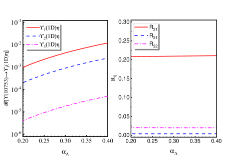
Figure 3: The $\alpha_{\Lambda}$ dependence of the calculated branching ratios $\mathcal{B}[\Upsilon(10753)\to\Upsilon(1^{3}D_{J})\eta]$ ($J=1,2,3$) (left panel) and the ratios $R_{ij}=\mathcal{B}[\Upsilon(10753)\to\Upsilon(1^{3}D_{i})\eta]/\mathcal{B}[\Upsilon(10753)\to\Upsilon(1^{3}D_{j})\eta]$ (right panel).

IV Discussion and conclusion

As a vector bottomonium candidate Wang:2018rjg , the recently reported $\Upsilon(10753)$ by Belle exists in the $e^{+}e^{-}\to\Upsilon(nS)\pi^{+}\pi^{-}$ ($n=1,2,3$) processes Belle:2019cbt . The $\Upsilon(10753)$ is a crucial state when constructing the bottomonium family. The study of its hidden-bottom decays is an important aspect to reflect the spectroscopy behavior of the $\Upsilon(10753)$ Li:2021jjt ; Bai:2022cfz . In this work, we calculate the $\Upsilon(10753)\to\Upsilon(1^{3}D_{J})\eta$ decays, which are involved in the observed $\Upsilon(1^{3}D_{2})$ BaBar:2010tqb and two missing bottomonia $\Upsilon(1^{3}D_{1})$ and $\Upsilon(1^{3}D_{3})$. Since the coupled-channel effect cannot be ignored for higher bottomonia Wang:2018rjg , we should introduce the hadronic loop mechanism when exploring the decay behavior of the $\Upsilon(10753)\to\Upsilon(1^{3}D_{J})\eta$ decays, and find that the $\Upsilon(10753)\to\Upsilon(1^{3}D_{1})\eta$ and $\Upsilon(10753)\to\Upsilon(1^{3}D_{2})\eta$ decay channels have sizable branching ratios. Thus, it is possible to find out these two predicted decay modes at Belle II. Different from these two decay channels, the $\Upsilon(10753)\to\Upsilon(1^{3}D_{3})\eta$ decay is suppressed. Thus, searching for $\Upsilon(10753)\to\Upsilon(1^{3}D_{3})\eta$ is not promising only if more data are accumulated in experiments.

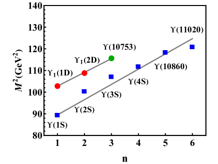
Figure 4: The Regge trajectories of the $\Upsilon(nS)$ and $\Upsilon_{1}(nD)$ series. Here, the blue squares denote the experimental data, the red cycles denote the averaged values of the predictions in Refs. Godfrey:2015dia ; Segovia:2016xqb ; Wang:2018rjg ; Deng:2016ktl and the green one is the measured mass of the $\Upsilon(10753)$. The trajectory slopes are determined as $\mu^{2}=7.0403$ GeV² and $6.3364$ GeV² for the $\Upsilon(nS)$ and $\Upsilon_{1}(nD)$ series, respectively.

In the following, we should discuss the mass spectrum of vector bottomonia. As listed in PDG ParticleDataGroup:2020ssz , there were $\Upsilon(1S)$, $\Upsilon(1S)$, $\Upsilon(3S)$, $\Upsilon(4S)$, $\Upsilon(10860)$, and $\Upsilon(11020)$. We find that they form a Regge trajectory as shown in Fig. 4. This Regge trajectory satisfies the relation $M^{2}=M_{0}^{2}+(n-1)\mu^{2}$ Regge:1959mz ; Regge:1960zc ; Chew:1961ev ; Chew:1962eu ; Collins:1971ff ; Anisovich:2000kxa ; Guo:2019wpx ; Guo:2022xqu . Here, $M_{0}$ is the mass of the ground state, $M$ denotes the mass of the radial excitation state with the radial quantum number $n$, and $\mu^{2}=7.0403$ GeV² is the slope of the Regge trajectory. Although the $\Upsilon(10753)$ is suggested as the mixture of $4S$ and $3D$ states of bottomonium, the $\Upsilon(10753)$ has main component of $3D$ state. Thus, we may take $\Upsilon(10753)$ and the predicted $\Upsilon(1^{3}D_{1})$ and $\Upsilon(2^{3}D_{1})$  Godfrey:2015dia ; Segovia:2016xqb ; Wang:2018rjg ; Deng:2016ktl to construct another Regge trajectory (see Fig. 4), which have slope $\mu^{2}=6.3364$ GeV². This slope is similar to that for the $S$-wave bottomonia. Thus, searching for the missing $\Upsilon(1^{3}D_{1})$ and $\Upsilon(2^{3}D_{1})$ bottononia in future experiment will be helpful to test this Regge trajectory behavior. It is obvious that the present work of studying the $\Upsilon(10753)\to\Upsilon(1^{3}D_{1})\eta$ shows the potential of finding out the $\Upsilon(1^{3}D_{1})$ bottomonium.

With running of Belle II, the physics relevant to the $\Upsilon(10753)$ should be paid more attention. Searching for different decay modes of the $\Upsilon(10753)$ is crucial step of establishing the $\Upsilon(10753)$ as bottomonium. We hope that the present work may provide valuable information to future experimental exploration.

Appendix A The Feynman rules for the interaction vertexes

In this appendix, the Feynman rules for the involved interaction vertexes are presented. The concrete information includes

$$\widehat{=} -g_{\Upsilon^{\prime}BB}\epsilon_{\Upsilon^{\prime}}^{\mu}(q_{1\mu}-q_{2\mu}),$$ (1.1)

$$\widehat{=} g_{\Upsilon^{\prime}BB^{*}}\varepsilon_{\alpha\beta\mu\nu}\epsilon_{\Upsilon^{\prime}}^{\mu}p^{\beta}(q_{2}^{\alpha}-q_{1}^{\alpha})\epsilon_{\bar{B}^{*}}^{*\nu},$$ (1.2)

$$\widehat{=} g_{\Upsilon^{\prime}BB^{*}}\varepsilon_{\alpha\beta\mu\nu}\epsilon_{\Upsilon^{\prime}}^{\mu}p^{\beta}(q_{1}^{\alpha}-q_{2}^{\alpha})\epsilon_{B^{*}}^{*\nu},$$ (1.3)

$$\widehat{=} -g_{\Upsilon_{1}^{\prime}BB}\epsilon_{\Upsilon_{1}^{\prime}}^{\mu}(q_{1\mu}-q_{2\mu}),$$ (1.4)

$$\widehat{=} g_{\Upsilon_{1}^{\prime}BB^{*}}\varepsilon_{\alpha\beta\mu\nu}\epsilon_{\Upsilon_{1}^{\prime}}^{\mu}p^{\beta}(q_{2}^{\alpha}-q_{1}^{\alpha})\epsilon_{\bar{B}^{*}}^{*\nu},$$ (1.5)

$$\widehat{=} g_{\Upsilon_{1}^{\prime}BB^{*}}\varepsilon_{\alpha\beta\mu\nu}\epsilon_{\Upsilon_{1}^{\prime}}^{\mu}p^{\beta}(q_{1}^{\alpha}-q_{2}^{\alpha})\epsilon_{B^{*}}^{*\nu},$$ (1.6)

$$\widehat{=} \begin{split}&-g_{\Upsilon_{1}^{\prime}B^{*}B^{*}}\epsilon_{\Upsilon_{1}^{\prime}}^{\mu}(-4g_{\alpha\beta}(q_{1\mu}-q_{2\mu})\\ &+g_{\alpha\mu}q_{1\beta}-g_{\beta\mu}q_{2\alpha})\epsilon_{B^{*}}^{*\alpha}\epsilon_{\bar{B}^{*}}^{*\beta},\end{split}$$ (1.7)

$$\widehat{=} -g_{BB^{*}\eta^{(\prime)}}p_{1}^{\alpha}\epsilon_{B^{*}\alpha}^{*},$$ (1.8)

$$\widehat{=} g_{BB^{*}\eta^{(\prime)}}p_{1}^{\alpha}\epsilon_{B^{*}\alpha},$$ (1.9)

$$\widehat{=} -g_{B^{*}B^{*}\eta^{(\prime)}}\varepsilon_{\mu\nu\alpha\beta}q_{1}^{\nu}q^{\mu}\epsilon_{B^{*}}^{\alpha}\epsilon_{B^{*}}^{*\beta}.$$ (1.10)

$$\widehat{=} g_{\Upsilon_{1}BB}\epsilon_{\Upsilon_{1}}^{*\mu}(q_{2\mu}-q{\mu}),$$ (1.11)

$$\widehat{=} g_{\Upsilon_{1}BB^{*}}\varepsilon_{\mu\nu\alpha\beta}p_{2}^{\nu}\epsilon_{\Upsilon_{1}}^{*\mu}\epsilon_{B^{*}}^{\alpha}(q^{\beta}-q_{2}^{\beta}),$$ (1.12)

$$\widehat{=} g_{\Upsilon_{1}BB^{*}}\varepsilon_{\mu\nu\alpha\beta}p_{2}^{\nu}\epsilon_{\Upsilon_{1}}^{*\mu}\epsilon_{\bar{B}^{*}}^{\alpha}(q_{2}^{\beta}-q^{\beta}),$$ (1.13)

$$\widehat{=} \begin{split}&g_{\Upsilon_{1}B^{*}B^{*}}\epsilon_{\Upsilon_{1}}^{*\mu}\epsilon_{B^{*}}^{\beta}\epsilon_{\bar{B}^{*}}^{\alpha}(g_{\alpha\mu}q_{2\beta}\\ &-g_{\beta\mu}q_{\alpha}+4g_{\alpha\beta}(q_{\mu}-q_{2\mu})),\end{split}$$ (1.14)

$$\widehat{=} -g_{\Upsilon_{2}BB^{*}}\epsilon_{\Upsilon_{2}}^{*\mu\nu}g_{\alpha\nu}\epsilon_{B^{*}}^{\alpha}(q_{\mu}-q_{2\mu}),$$ (1.15)

$$\widehat{=} g_{\Upsilon_{2}BB^{*}}\epsilon_{\Upsilon_{2}}^{*\mu\nu}g_{\alpha\nu}\epsilon_{\bar{B}^{*}}^{\alpha}(q_{\mu}-q_{2\mu}),$$ (1.16)

$$\widehat{=} \begin{split}&g_{\Upsilon_{2}B^{*}B^{*}}\varepsilon_{\kappa\lambda\xi\nu}p_{2}^{\lambda}\epsilon_{\Upsilon_{2}}^{*\mu\nu}(q^{\kappa}-q_{2}^{\kappa})\\ &\times(g_{\alpha\mu}g_{\beta}^{\xi}+g_{\alpha}^{\xi}g_{\beta\mu})\epsilon_{B^{*}}^{\beta}\epsilon_{\bar{B}^{*}}^{\alpha},\end{split}$$ (1.17)

$$\widehat{=} \begin{split}&-g_{\Upsilon_{3}B^{*}B^{*}}\epsilon_{\Upsilon_{3}}^{*\mu\nu\rho}(g_{\alpha\nu}g_{\beta\rho}+g_{\alpha\rho}g_{\beta\nu})\\ &\times(q_{\mu}-q_{2\mu})\epsilon_{B^{*}}^{\beta}\epsilon_{\bar{B}^{*}}^{\alpha}.\end{split}$$ (1.18)

References

• (1) E. Kou et al. [Belle-II], The Belle II Physics Book, PTEP 2019 (2019) no.12, 123C01 [erratum: PTEP 2020 (2020) no.2, 029201].
• (2) R. Mizuk et al. [Belle], Observation of a new structure near 10.75 GeV in the energy dependence of the $e^{+}e^{-}\to\Upsilon(nS)\pi^{+}\pi^{-}$ (n = 1, 2, 3) cross sections, JHEP 10 (2019), 220.
• (3) P. A. Zyla et al. [Particle Data Group], Review of Particle Physics, PTEP 2020 (2020) no.8, 083C01.
• (4) S. Godfrey and K. Moats, Bottomonium Mesons and Strategies for their Observation, Phys. Rev. D 92 (2015) no.5, 054034.
• (5) J. Segovia, P. G. Ortega, D. R. Entem and F. Fernández, Bottomonium spectrum revisited, Phys. Rev. D 93 (2016) no.7, 074027.
• (6) J. Z. Wang, Z. F. Sun, X. Liu and T. Matsuki, Higher bottomonium zoo, Eur. Phys. J. C 78 (2018) no.11, 915.
• (7) Z. G. Wang, Vector hidden-bottom tetraquark candidate: $Y(10750)$, Chin. Phys. C 43 (2019) no.12, 123102.
• (8) A. Ali, L. Maiani, A. Parkhomenko and W. Wang, Tetraquark Interpretation and Production Mechanism of the Belle $Y_{b}(10750)$-Resonance, PoS ICHEP2020 (2021), 493.
• (9) J. Tarrús Castellà and E. Passemar, Exotic to standard bottomonium transitions, Phys. Rev. D 104 (2021) no.3, 034019.
• (10) P. Bicudo, M. Cardoso, N. Cardoso and M. Wagner, Bottomonium resonances with $I=0$ from lattice QCD correlation functions with static and light quarks, Phys. Rev. D 101 (2020) no.3, 034503.
• (11) P. Bicudo, N. Cardoso, L. Müller and M. Wagner, Computation of the quarkonium and meson-meson composition of the $\Upsilon(nS)$ states and of the new $\Upsilon(10753)$ Belle resonance from lattice QCD static potentials, Phys. Rev. D 103 (2021) no.7, 074507.
• (12) Y. S. Li, Z. Y. Bai, Q. Huang and X. Liu, Hidden-bottom hadronic decays of $\Upsilon(10753)$ with a $\eta^{(\prime)}$ or $\omega$ emission, Phys. Rev. D 104 (2021) no.3, 034036.
• (13) Z. Y. Bai, Y. S. Li, Q. Huang, X. Liu and T. Matsuki, $\Upsilon(10753)\to\Upsilon(nS)\pi^{+}\pi^{-}$ decays induced by hadronic loop mechanism, Phys. Rev. D 105 (2022) no.7, 074007.
• (14) C. Meng and K. T. Chao, Scalar resonance contributions to the dipion transition rates of $\Upsilon(4S,5S)$ in the re-scattering model, Phys. Rev. D 77 (2008), 074003.
• (15) C. Meng and K. T. Chao, Peak shifts due to $B^{*}\bar{B}^{*}$ rescattering in $\Upsilon(5S)$ dipion transitions, Phys. Rev. D 78 (2008), 034022.
• (16) C. Meng and K. T. Chao, $\Upsilon(4S,5S)\to\Upsilon(1S)\eta$ transitions in the rescattering model and the new BaBar measurement, Phys. Rev. D 78 (2008), 074001.
• (17) D. Y. Chen, X. Liu and X. Q. Li, Anomalous dipion invariant mass distribution of the $\Upsilon(4S)$ decays into $\Upsilon(1S)\pi^{+}\pi^{-}$ and $\Upsilon(2S)\pi^{+}\pi^{-}$, Eur. Phys. J. C 71 (2011), 1808.
• (18) D. Y. Chen, J. He, X. Q. Li and X. Liu, Dipion invariant mass distribution of the anomalous $\Upsilon(1S)\pi^{+}\pi^{-}$ and $\Upsilon(2S)\pi^{+}\pi^{-}$ production near the peak of $\Upsilon(10860)$, Phys. Rev. D 84 (2011), 074006.
• (19) D. Y. Chen, X. Liu and S. L. Zhu, Charged bottomonium-like states $Z_{b}(10610)$ and $Z_{b}(10650)$ and the $\Upsilon(5S)\to\Upsilon(2S)\pi^{+}\pi^{-}$ decay, Phys. Rev. D 84 (2011), 074016.
• (20) D. Y. Chen, X. Liu and T. Matsuki, Explaining the anomalous $\Upsilon(5S)\to\chi_{bJ}\omega$ decays through the hadronic loop effect, Phys. Rev. D 90 (2014) no.3, 034019.
• (21) B. Wang, X. Liu and D. Y. Chen, Prediction of anomalous $\Upsilon(5S)\to\Upsilon(1^{3}D_{J})\eta$ transitions, Phys. Rev. D 94 (2016) no.9, 094039.
• (22) Q. Huang, B. Wang, X. Liu, D. Y. Chen and T. Matsuki, Exploring the $\Upsilon(6S)\rightarrow\chi_{bJ}\phi$ and $\Upsilon(6S)\rightarrow\chi_{bJ}\omega$ hidden-bottom hadronic transitions, Eur. Phys. J. C 77 (2017) no.3, 165.
• (23) Y. Zhang and G. Li, Exploring the $\Upsilon(4S,5S,6S)\to h_{b}(1P)\eta$ hidden-bottom hadronic transitions, Phys. Rev. D 97 (2018) no.1, 014018.
• (24) Q. Huang, X. Liu and T. Matsuki, Proposal of searching for the $\Upsilon(6S)$ hadronic decays into $\Upsilon(nS)$ plus $\eta^{(\prime)}$, Phys. Rev. D 98 (2018) no.5, 054008.
• (25) Q. Huang, H. Xu, X. Liu and T. Matsuki, Potential observation of the $\Upsilon(6S)\to\Upsilon(1^{3}D_{J})\eta$ transitions at Belle II, Phys. Rev. D 97 (2018) no.9, 094018.
• (26) A. M. Badalian, B. L. G. Bakker and I. V. Danilkin, On the possibility to observe higher $n^{3}D_{1}$ bottomonium states in the $e^{+}e^{-}$ processes, Phys. Rev. D 79 (2009), 037505.
• (27) A. M. Badalian, B. L. G. Bakker and I. V. Danilkin, Dielectron widths of the $S$-, $D$-vector bottomonium states, Phys. Atom. Nucl. 73 (2010), 138-149.
• (28) W. H. Liang, N. Ikeno and E. Oset, $\Upsilon(nl)$ decay into $B^{(*)}\bar{B}^{(*)}$, Phys. Lett. B 803 (2020), 135340.
• (29) M. P. Locher, Y. Lu and B. S. Zou, Rates for the reactions $\bar{p}p\to\pi\phi$ and $\gamma\phi$, Z. Phys. A 347 (1994), 281-284.
• (30) X. Q. Li, D. V. Bugg and B. S. Zou, A Possible explanation of the “$\rho\pi$ puzzle” in $J/\psi$, $\psi^{\prime}$ decays, Phys. Rev. D 55 (1997), 1421-1424.
• (31) H. Y. Cheng, C. K. Chua and A. Soni, Final state interactions in hadronic B decays, Phys. Rev. D 71 (2005), 014030.
• (32) O. Gortchakov, M. P. Locher, V. E. Markushin and S. von Rotz, Two meson doorway calculation for $\bar{p}p\to\phi\pi$ including off-shell effects and the OZI rule, Z. Phys. A 353 (1996), 447-453.
• (33) X. Liu, X. Q. Zeng and X. Q. Li, Study on contributions of hadronic loops to decays of $J/\psi\to$ vector + pseudoscalar mesons, Phys. Rev. D 74 (2006), 074003.
• (34) X. Liu, B. Zhang and X. Q. Li, The Puzzle of excessive non-$D\bar{D}$ component of the inclusive $\psi(3770)$ decay and the long-distant contribution, Phys. Lett. B 675 (2009), 441-445.
• (35) G. Li, X. h. Liu, Q. Wang and Q. Zhao, Further understanding of the non-$D\bar{D}$ decays of $\psi(3770)$, Phys. Rev. D 88 (2013) no.1, 014010.
• (36) R. Casalbuoni, A. Deandrea, N. Di Bartolomeo, R. Gatto, F. Feruglio and G. Nardulli, Phenomenology of heavy meson chiral Lagrangians, Phys. Rept. 281 (1997), 145-238.
• (37) M. B. Wise, Chiral perturbation theory for hadrons containing a heavy quark, Phys. Rev. D 45 (1992) no.7, R2188.
• (38) H. Xu, X. Liu and T. Matsuki, Understanding $B^{-}\rightarrow X(3823)K^{-}$ via rescattering mechanism and predicting $B^{-}\to\eta_{c2}(^{1}D_{2})/\psi_{3}(^{3}D_{3})K^{-}$, Phys. Rev. D 94 (2016) no.3, 034005.
• (39) M. X. Duan, J. Z. Wang, Y. S. Li and X. Liu, Role of the newly measured $B\to KD\bar{D}$ process to establish $\chi_{c0}(2P)$ state, Phys. Rev. D 104 (2021) no.3, 034035.
• (40) P. del Amo Sanchez et al. [BaBar], Observation of the $\Upsilon(1^{3}D_{J})$ Bottomonium State through Decays to $\pi^{+}\pi^{-}\Upsilon{1S}$, Phys. Rev. D 82 (2010), 111102.
• (41) J. Jousset et al. [DM2], The $J/\psi\to$ Vector + Pseudoscalar Decays and the $\eta$, $\eta^{\prime}$ Quark Content, Phys. Rev. D 41 (1990), 1389.
• (42) U. Tamponi et al. [Belle], Inclusive study of bottomonium production in association with an $\eta$ meson in $e^{+}e^{-}$ annihilations near $\varUpsilon(5S)$, Eur. Phys. J. C 78, no.8, 633 (2018).
• (43) T. Regge, Introduction to complex orbital momenta, Nuovo Cim. 14 (1959), 951.
• (44) T. Regge, Bound states, Shadow states and Mandelstam representation, Nuovo Cim. 18 (1960), 947-956.
• (45) G. F. Chew and S. C. Frautschi, Principle of Equivalence for All Strongly Interacting Particles Within the S Matrix Framework, Phys. Rev. Lett. 7 (1961), 394-397.
• (46) G. F. Chew and S. C. Frautschi, Regge Trajectories and the Principle of Maximum Strength for Strong Interactions, Phys. Rev. Lett. 8 (1962), 41-44.
• (47) P. D. B. Collins, Regge theory and particle physics, Phys. Rept. 1 (1971), 103-234.
• (48) A. V. Anisovich, V. V. Anisovich and A. V. Sarantsev, Systematics of $q\bar{q}$ states in the $(n,M^{2})$ and $(J,M^{2})$ planes, Phys. Rev. D 62 (2000), 051502.
• (49) D. Guo, C. Q. Pang, Z. W. Liu and X. Liu, Study of unflavored light mesons with $J^{PC}=2^{--}$, Phys. Rev. D 99 (2019) no.5, 056001.
• (50) D. Guo, W. Chen, H. X. Chen, X. Liu and S. L. Zhu, Newly observed $a_{0}(1817)$ as the scaling point of constructing the scalar meson spectroscopy, [arXiv:2204.13092 [hep-ph]].
• (51) W. J. Deng, H. Liu, L. C. Gui and X. H. Zhong, Spectrum and electromagnetic transitions of bottomonium, Phys. Rev. D 95 (2017) no.7, 074002.