A Comparative Tutorial of Bayesian Sequential Design and Reinforcement Learning

Abstract

Reinforcement Learning (RL) is a computational approach to reward-driven learning in sequential decision problems. It implements the discovery of optimal actions by learning from an agent interacting with an environment rather than from supervised data. We contrast and compare RL with traditional sequential design, focusing on simulation-based Bayesian sequential design (BSD). Recently, there has been an increasing interest in RL techniques for healthcare applications. We introduce two related applications as motivating examples. In both applications, the sequential nature of the decisions is restricted to sequential stopping. Rather than a comprehensive survey, the focus of the discussion is on solutions using standard tools for these two relatively simple sequential stopping problems. Both problems are inspired by adaptive clinical trial design. We use examples to explain the terminology and mathematical background that underlie each framework and map one to the other. The implementations and results illustrate the many similarities between RL and BSD. The results motivate the discussion of the potential strengths and limitations of each approach.

1 Introduction

Sequential design problems (SDP) involve a sequence of decisions $D_{t}$ with data $Y_{t}$ observed at every time step $t=1,\ldots,T$ (DeGroot, 2004; Berger, 2013). The goal is to find a decision rule $(Y_{1},\ldots,Y_{t})\mapsto D_{t}$ that maximizes the expected value of a utility function. The utility function encodes an agent’s preferences as a function of hypothetical future data and assumed truth. The decision rule is prescribed before observing future data beyond $Y_{t}$ – as the term “design” emphasizes – assuming a probabilistic model with unknown parameters $\theta$ that generate the future data. For example, $\theta$ can be the true effect of a drug. Figure 1a summarizes the setup of a general SDP. As motivating examples in the upcoming discussion we will use two examples of clinical trial design, which naturally give rise to SDPs (Rossell et al., 2007; Berry and Ho, 1988; Christen and Nakamura, 2003). Both examples are about sequential stopping, that is, the sequential decision is to determine when and how to end the study. Figure 1b shows the setup of sequential stopping problems.

Using these examples, we compare two families of simulation-based methods for solving SDPs with applications in sequential stopping. The first is simulation-based Bayesian Sequential Design (BSD) (Müller et al., 2007), which is based on Bayesian decision theory (Berger, 2013). The other approach is Reinforcement Learning (RL), a paradigm based on the interaction between an agent and an environment that results in potential rewards (or costs) for each decision. RL has recently been proposed as a method to implement SDPs focusing on recent advances in deep learning (Shen and Huan, 2021), outside the context of clinical studies. Earlier application of RL related to clinical study design can be found in the dynamic treatment regimes literature (Zhao et al., 2009; Murphy, 2003; Murphy et al., 2007). There is a longstanding literature on such problems in statistics; see the review by Parmigiani and Inoue (2009, chapter 15) and the references therein. Implementing RL and BSD in these two motivating example problems (using standard algorithms) will illustrate many similarities between the two frameworks, while highlighting the potential strengths and limitations of each paradigm.

A note about the scope of the upcoming discussion. It is meant to highlight the similarities and differences of algorithms in BSD and RL, and we provide a (partial) mapping of notations. There is no intent to provide (yet another) review of BSD or RL and its many variations. This article focuses on a few variations that best contrast the two traditions, and we try to highlight the relative advantages of each method. In short, BSD is better equipped to deal with additional structure, that is, to include more details in the inference model. For example, dealing with delayed responses in a clinical study, one might want to include a model to use early responses to predict such delayed outcomes. Or one might want to borrow strength across multiple related problems. Doing so would also be possible in RL, but it requires to leave the framework of Markov decision processes underlying many RL algorithms (Gaon and Brafman, 2020), and discussed below. On the other hand, RL allows computation-efficient implementations, and is routinely used for much larger scale problems than BSD. The availability of computation-efficient implementations is critical in applications where sequential designs need to be evaluated for summaries under (hypothetical) repeated experimentation. This is the case, for example, in clinical trial design when frequentist error rates and power need to be reported. The evaluation requires Monte Carlo experiments with massive repeat simulations, making computation-efficient implementation important.

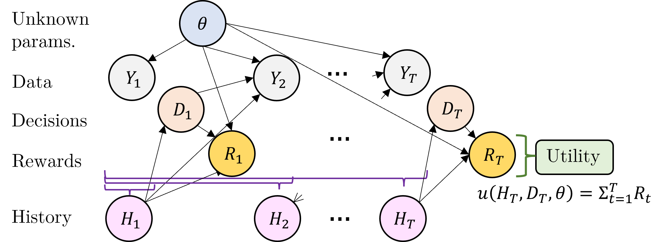
(a) Generic SDP.

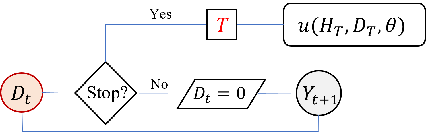
(b) Sequential stopping.

Figure 1: Panel (a) shows the directed graph of a general SDP problem. In the figure, $H_{t}=\{Y_{1},D_{1},Y_{2},\ldots,D_{t-1},Y_{t}\}$ denotes the history or information set at decision time $t$. There is an implicit arrow from every element of $H_{t}$ onto $D_{t}$, summarily implied by the arrow $H_{t}\to D_{t}$. In RL the utility function is usually written as a sum $G=\sum_{t=1}^{T}R_{t}$ of immediate rewards $R_{t}(H_{t},D_{t})$ (although it is usually called the return instead of the utility). Panel (b) shows a flow chart for the special case of sequential stopping problems, with $D_{t}=0$ indicating continuation. The node ${\color[rgb]{1,0,0}T}$ represents stopping the trial ($t=T$ and $D_{T}\neq 0$).

BSD:

BSD is a model-based paradigm for SDPs based on a sampling model $p(Y_{t}\mid H_{t-1},D_{t-1},\theta)$ for the observed data and a prior $p(\theta)$ reflecting the agent’s uncertainty about the unknown parameters.

To compare alternative decisions $D_{t}$, the agent uses an optimality criterion that is formalized as a utility function $u(Y_{1},\ldots,Y_{T},D_{1},\ldots,D_{T},\theta)$ which quantifies the agent’s preferences under hypothetical data, decisions and truth. It will be convenient to write the utility as $u(H_{T},D_{T}=d,\theta)$, where $H_{t}$ denotes the history $H_{t}:=(Y_{1},D_{1},\ldots,D_{t-1},Y_{t})$ at decision time $t$. Rational decision makers should act as if they were to maximize such utility in expectation conditioning on already observed data, and marginalizing with respect to any (still) unknown quantities like future data or parameters (DeGroot, 2004).

To develop a solution strategy, we start at time $T$ (final horizon or stopping time). Denote by $U(H_{T},d)=E\{u(H_{T},D_{T}=d,\theta)\mid H_{T}\}$ the expected utility at the stopping time $T$. Then, the rational agent would select $D^{\star}_{T}(H_{T})=\operatorname*{arg\,max}_{d}U(H_{T},d)$ at the stopping time. For earlier time steps, rational decisions derive from expectations over future data, with later optimal decisions plugged in,

$$U(H_{t},d)=E\{u(H_{t},D_{t}=d,Y_{t+1}(D_{t}=d),D^{\star}_{t+1}(H_{t+1}(D_{t}=d)),\ldots,D^{\star}_{T}(H_{T}(D_{t}=d)),\theta\mid H_{t}\}$$ (1)

which determine the optimal decision (“Bayes rule”) as

$$D^{\star}_{t}(H_{t})=\textstyle{\operatorname*{arg\,max}_{d}\,}U(H_{t},d).$$ (2)

Here, we use a potential outcomes notation $H_{t+1}(D_{t}=d)$ to emphasize that future history depends on the action $D_{t}=d$ (Robins, 1997), and similarly for other quantities. In the notation for expected utility $U(\cdot)$, the lack of an argument indicates marginalization (with respect to future data and parameters) and optimization (with respect to future actions), respectively. For example, in (1) expected utility conditions on $H_{t}$, but marginalizes w.r.t. future data $Y_{t+k}$ and substitutes optimal future decisions $D^{\star}_{t+k}$.

Some readers, especially those familiar with RL, might wonder why $D_{t}=d$ does not appear on the right-hand side of the conditional expectation (as in RL’s state-action value functions). This is because in the BSD framework actions are deterministic. There is no good reason why a rational decision maker would randomize (Berger, 2013). However, note that in clinical studies randomization is usually included and desired, but for other reasons – not to achieve an optimal decision, but to facilitate attribution of differences in outcomes to the treatment selection.

RL

RL addresses a wider variety of sequential problems than BSD, provided one can formulate them as an agent interacting with an environment yielding rewards $R_{t}$ at every time step. Environments can be based on simulations. For example, popular successful RL applications with simulation-based environments include Atari video-games (Mnih et al., 2013), complex board games like chess and Go (Silver et al., 2018), robotic tasks (Tunyasuvunakool et al., 2020) and autonomous driving (Wurman et al., 2022; Sallab et al., 2017).

Just as in BSD, the interactive setup for RL (transition and rewards) can be defined by a sampling model and a prior over $\theta$. The interaction replicates the decision process, shown in Figure 1. Each draw $\theta\sim p(\theta)$ constitutes a new instance or episode of the environment. The RL agent seeks to maximize the expected sum of rewards $G=\sum_{t=1}^{T}R_{t}$, known as the return, over an episode. The return $G$ is the analogue of the utility function.

Decision rules are called policies in RL. A (stochastic) policy maps an observed history to a distribution over actions $D_{t}\sim\pi(\cdot\mid H_{t})$. The optimal policy ${\pi_{\star}}$ satisfies ${\pi_{\star}}=\operatorname*{arg\,max}_{\pi}E\{G\mid\pi\}$. As mentioned before, the notion of stochastic policies is not natural in BSD with its focus on decisions that a rational agent would take. In fact, under some regularity conditions it can be shown that also the optimal RL policy is deterministic (Puterman, 2014). So why stochastic policies? Stochastic policies in RL serve to implement exploration. In BSD it is assumed that if exploration were called for, it would be recognized by the optimal decision rule. While in theory this is the case, in practice additional reinforcement of exploration is reasonable. Also, as we shall see later, the use of stochastic policies facilitates the search for optimal policies by allowing the use of the stochastic gradient theorem.

Another close similarity of BSD and RL occurs in the definition of expected utility and the state-action value function in RL. The state-action value function is $Q^{\pi}(H_{t},d)=E\{\sum_{k=t}^{T}R_{k}\mid H_{t},D_{t}=d,\pi\}$. The value function of the optimal policy $Q^{{\pi_{\star}}}(H_{t},d)$ plays the same role as expected utility $U(H_{t},d)$ when optimal decisions are substituted for future decisions $D_{s}$, $s>t$. An important difference is the stochastic nature of $\pi$ in the state-value function, versus the deterministic decisions $D_{t}$ in BSD.

From this brief introduction one can already notice many correspondences between the objects in RL and BSD. Table 1 shows a partial mapping between their respective terminologies. Not all are perfect equivalences. Sometimes common use in BSD and RL involves different levels of marginalization and/or substituting optimal values. Some of the analogies in the table will be developed in the remainder of the paper.

Table 1: A brief comparison of key quantities in BSD and RL. Variations without time subindex _t refer to time-invariant versions. Using states $S_{t}$, in many instances an argument $H_{t}$ can be replaced by $S_{t}$, as in $D_{t}(S_{t})$, We use $Y=(Y_{1},\ldots,Y_{T})$ etc. to refer to lists over $t=1,\ldots,T$.

	BSD	RL
$Y_{t}$	data observed at time $t$
$H_{t}=(Y_{1},D_{1}\ldots D_{t-1},Y_{t})$	history (information set) at decision time $t$
$D_{t}=D_{t}(H_{t})$	action (decision) at time $t$
$S_{t}=S_{t}(H_{t})$	summary (sufficient) statistic	state
$D_{\phi,t}$	(deterministic) action at time $t$	n/a (a)
	indexed by parameter $\phi$ (policy)
$\pi(D_{t}\mid H_{t})$	n/a (no randomization)	(random) policy
$\pi_{\phi}$	n/a	policy indexed by $\phi$
optimal decision/policy	Bayes rule $D^{\star}(H_{t})$ (2)	optimal policy ${\pi_{\star}}(H_{t})$
$\theta$	unknown parameter
	(usually) required	optional
$R_{t}$	n/a (b)	(immediate) reward at time $t$
optimality criterion	utility $u(Y,D,\theta)=u(H_{t},D_{t},\theta)$	total return $G=\sum_{k=1}^{T}R_{t}$ or
		remaining return $G_{t}=\sum_{k=t}^{T}R_{k}$
state-action value	n/a (deterministic $D^{\star}$)	$Q^{\pi}(H_{t},D_{t})=E_{\pi}\{G_{t}\mid H_{t},D_{t}\}$
state value	n/a (deterministic $D^{\star}$)	$V^{\pi}(H_{t})=E_{\pi}\{G_{t}\mid H_{t},\pi\}$
value under optimal	$U(H_{t},D_{t})$	$Q^{{\pi_{\star}}}(H_{t},D_{t})$
future actions
optimal value	$U(H_{t},D^{\star}(H_{t}))$	$V^{{\pi_{\star}}}(H_{t})$
$J(\phi)$	expectation under policy/decision indexed by $\phi$
	$=E\{u(Y,D_{\phi},\theta)\}$	$=E\{G\mid\pi_{\phi}\}$
Bellman equation/	$U(H_{t},D_{t})=$	$Q^{\pi}(H_{t},D_{t})=$
backward induction	$E\{U(H_{t+1}(D_{t}))\mid H_{t}\}$	$E\{R_{t}+V^{\pi}(H_{t+1})\mid H_{t},D_{t},\pi\}$

^(a) deterministic policies $\pi_{\phi}(H_{t})$ are not discussed in this review, but see Silver et al. (2014).
^(b) additive decomposition as $u(H_{T},D_{t},\theta)=\sum_{t}R(H_{t},D_{t},\theta)$ is possible, but not usually made explicit.

2 Two examples of optimal stopping in clinical trials

The two stylized examples introduced here mimic sequential stopping in a clinical trial. The agent is an investigator who is planning and overseeing the trial. The data $Y_{t}$ are clinical outcomes recorded for each patient. In both cases $D_{t}$ refers to a stopping decision after $t$ (cohorts of) patients. Under continuation ($D_{t}=0$), the agent incurs an additional cost $c_{t}$ for recruiting the next cohort of patients. Under stopping ($D_{t}\neq 0$), on the other hand, the agent incurs a cost if a wrong (precise meaning to be specified) recommendation is made. At each time the agent has to choose between continuing the study – to learn more – versus stopping and realizing a reward for a good final recommendation (about the treatment). Throughout we use the notions of cost (or loss) and utility interchangeably, treating loss as negative utility.

Example 1: A binary hypothesis

Consider the decision problem of choosing between $H_{1}:\theta=\theta_{1}$ and $H_{2}:\theta=\theta_{2}$. For instance, $\theta$ could represent the probability of a clinical response for an experimental therapy. Assume a binary outcome $Y_{t}$ with a Bernoulli sampling model $p(Y_{t}=1\mid\theta)=\theta$ and a discrete two-point prior $p(\theta=\theta_{1})=p(\theta=\theta_{2})=\frac{1}{2}$.

The possible decisions at any time are $D_{t}\in\{0,1,2\}$. Here $D_{t}=0$ indicates continuation, $D_{t}=1$ indicates to terminate the trial and report $H_{1}(\theta=\theta_{1})$, and $D_{t}=2$ means terminate and report $H_{2}(\theta=\theta_{2})$. The utility function includes a (fixed) sampling cost $c$ for each cohort and a final cost $K>0$ for reporting the wrong hypothesis. The utility function is

$$u(H_{T},D_{T},\theta)=-cT-K\,\mathbb{I}(\theta\neq\theta_{D_{T}}).$$ (3)

The relevant history $H_{t}$ can be represented using the summary statistic $S_{t}=(t,\sum_{k\leq t}Y_{k}/t)$, since this statistic is sufficient for the posterior of $\theta$. The implementations of simulation-based BSD and RL use this summary statistic. The problem parameters are fixed as $c=1$ and $K=100$. Example trajectories of $S_{t}$ assuming no stopping are shown in Figure 2(a).

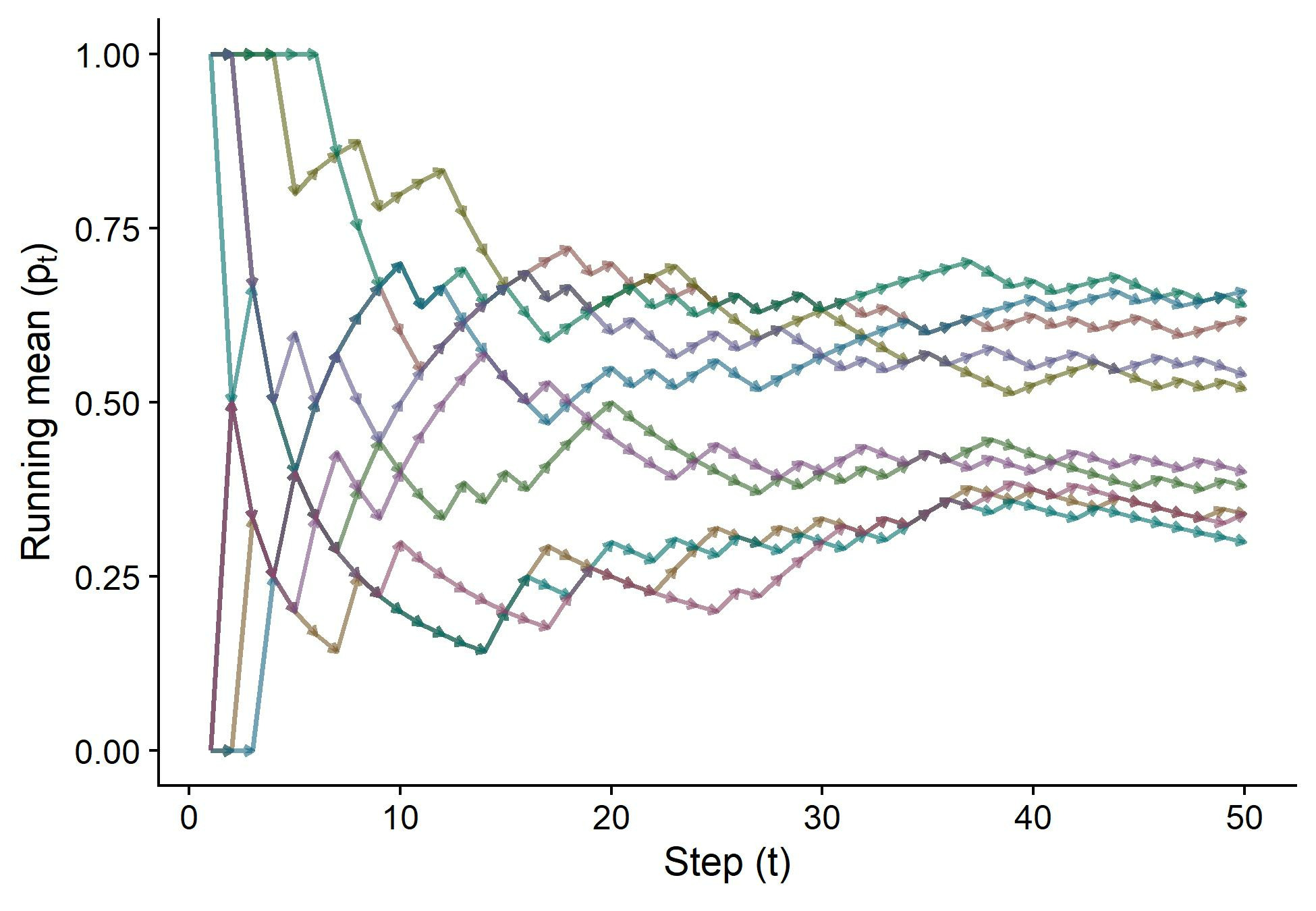
(a) Example 1: trajectories

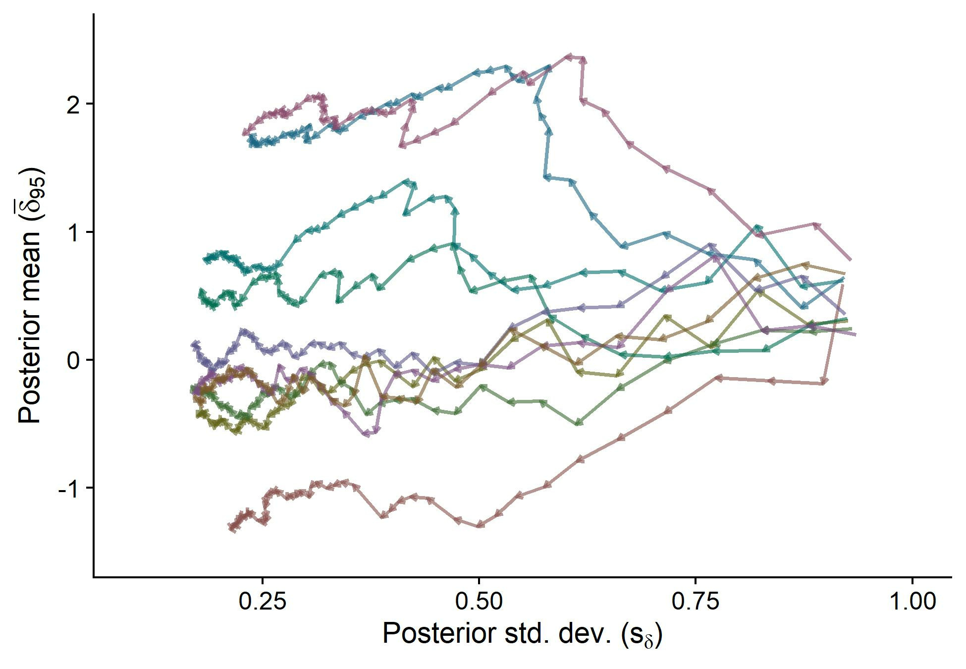
(b) Example 2: trajectories

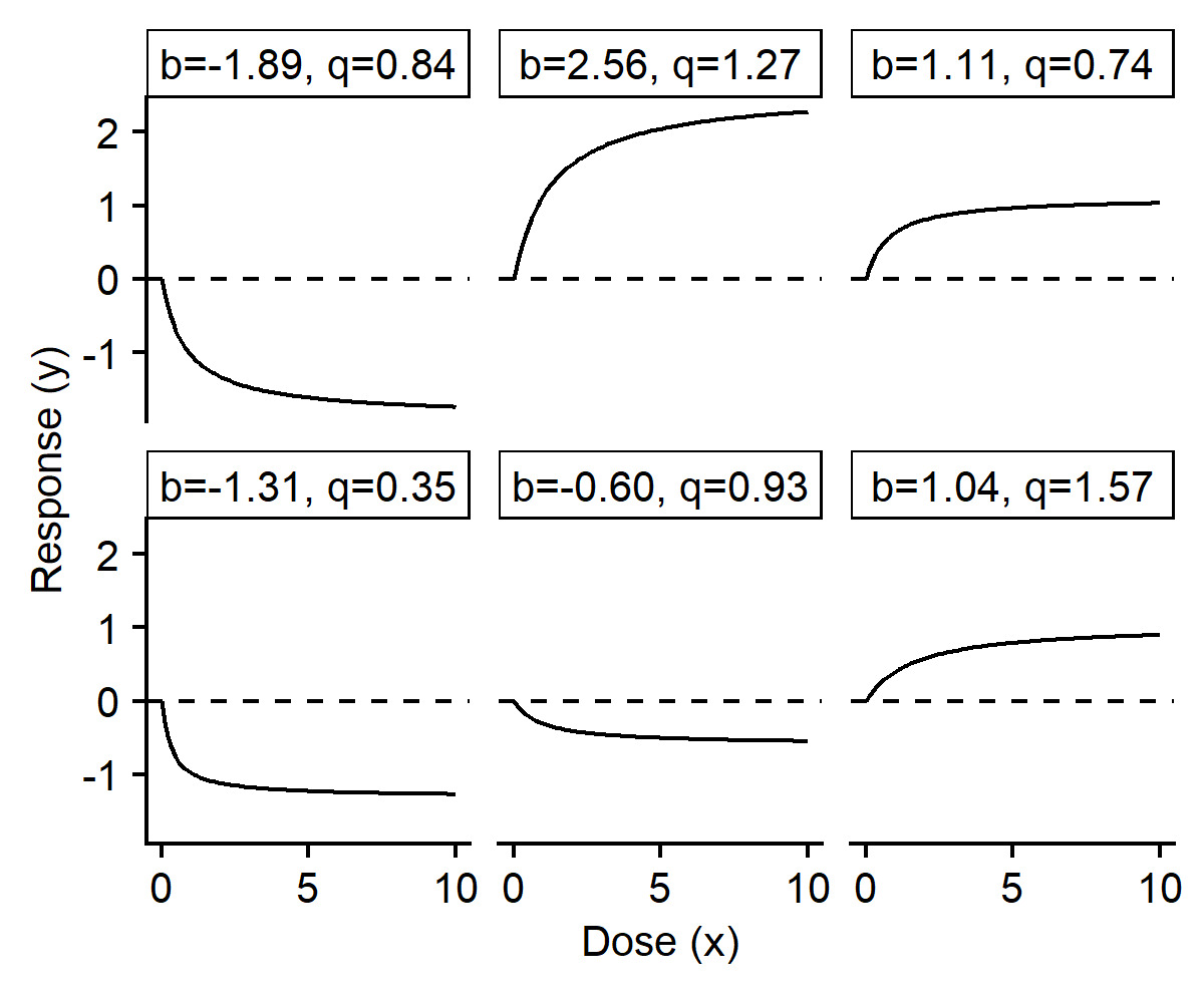
(c) Example 2: dose-response models

Figure 2: Data from the two sequential stopping examples. (a) and (b) are forward simulations assuming no stopping; (c) shows the implied dose-response curves for different random draws of the prior.

Example 2: A dose-finding study

This example is a stylized version of the ASTIN trial (Grieve and Krams, 2005). The trial aims to find the optimal dose for a drug from a set of candidate doses ${\mathbb{X}}=\{{\textnormal{x}}_{0},\ldots,{\textnormal{x}}_{G}\}$ where ${\textnormal{x}}_{0}=0$ stands for placebo. At each time $t$, a dose $X_{t}\in{\mathbb{X}}$ is assigned to the next patient (cohort), and an efficacy outcome $Y_{t}$ is observed. The aim is to learn about the dose-response curve $f(X_{t})=\mathbb{E}(Y_{t}\mid X_{t})$, and more specifically, to find the dose ${\textnormal{x}}_{95}$ (the ED95) that achieves 95% of the maximum possible improvement over placebo. Let $\delta_{g}=f({\textnormal{x}}_{g})-f({\textnormal{x}}_{0})$ be the advantage over the placebo at dose ${\textnormal{x}}_{g}$. We set up a nonlinear regression $Y_{t}=f(X_{t}\mid\theta)+\epsilon_{t}$ with $\epsilon_{t}\sim N(0,\sigma^{2})$ using a dose-response function

$$f({\textnormal{x}}\mid\theta)=a+b\frac{{\textnormal{x}}^{r}}{(q^{r}+{\textnormal{x}}^{r})}$$ (4)

with $\theta=(a,b,q,r)$ and a prior $p(\theta)=N(\theta_{0},diag(\lambda_{0}^{2}))$. In the PK/PD (pharmacokinetics/pharmacodynamics) literature model (4) is known as the $E_{max}$ model (Meibohm and Derendorf, 1997).

Similar to Example 1, $D_{t}\in\{0,1,2\}$ with $D_{t}=0$ indicating continuation, $D_{t}=1$ indicating stopping the trial and recommending no further investigation of the experimental therapy, and $D_{t}=2$ indicating stopping and recommending for a follow-up trial set up as a pivotal trial to test the null hypothesis $H_{0}:$ $\delta_{95}=0$. If continuing the trial, the next assigned dose is $X_{t+1}=\min\{X_{t}+\xi,\hat{x}_{95,t}\}$ where $\hat{x}_{95,t}$ is the latest estimate of the ED95, and $\xi$ is a maximum allowable dose escalation between cohorts. If requiring a pivotal trial, $N_{\alpha,\beta}$ patients are assigned to the dose $\hat{x}_{95,T}$, with $N_{\alpha,\beta}$ computed from the observed data to achieve a desired power $1-\beta$ at a certain alternative $H_{1}:\theta=\theta_{1}$ for test of size $\alpha$. Details are given in Appendix A.

The utility function includes a patient recruitment cost of $c$ and a prize $K>0$ if the null hypothesis $H_{0}(\delta_{95}=0)$ is rejected in the pivotal trial (meaning the agent found evidence of an effective drug). Denote $\Delta_{R}=\Pr(\mbox{reject $H_{0}$ in the 2nd trial}\mid H_{T})$. At the stopping time $T=\min_{t}\{D_{t}\neq 0\}$, utility is calculated as

$$u(H_{T},D_{T},\theta)=\begin{cases}-cT&\mbox{if }D_{T}=1\\ -cT+\left\{-cN_{\alpha,\beta}(H_{T})+K\Delta_{R}(H_{T})\right\}&\mbox{if }D_{T}=2\end{cases}$$ (5)

In our implementation we fix $a=0,r=1,\sigma=1$ in (4) and $c=1,K=100$ in (5), and $\xi=1$, leaving the unknown parameters $\theta=(b,q)$, including the maximum effect $b$ and the location of the ${\textnormal{x}}_{50}$. The prior of $\theta$ has mean $\theta_{0}=(1/2,1)$ with variances $\lambda_{0}=(1,1)$ and we add the constraint $q\geq 0.1$.

The summary statistic is $S_{t}=(\bar{\delta}_{95},s_{\delta})$ where $\bar{\delta}_{95}$ and $s_{\delta}$ are posterior mean and standard deviation of $\delta_{95}$. Figure 2(b) shows examples of trajectories of these summaries until some maximum time horizon $T$ (i.e., assuming no stopping). The trajectories are created by sampling $\theta$ from the prior, assigning doses as described, and sampling responses using (4). Figure 2(c) shows examples of the implied dose-response curve $f({\textnormal{x}}\mid\theta)$ for different prior draws. Notice that the chosen summaries do not capture the full posterior. The statistic $S_{t}$ is not a sufficient statistic for the posterior. However, as shown in Appendix A, $N_{\alpha,\beta}$ and $\Delta_{R}$, and therefore the utility, depend on the data only through $S_{t}$.

3 Simulation-based Bayesian sequential design

From the expected utility definition in (1), one immediately deduces that

$$U(H_{t},D_{t}=d)=E\{U(H_{t+1}(D_{t}=d),D^{\star}(H_{t+1}(D_{t}=d)))\mid H_{t}\},$$ (6)

with the expectation being with respect to future data and $\theta$, and substituting optimal choices for future decisions, $s>t$. In words, for a rational agent taking optimal actions, the expected utility given history $H_{t}$ must be the same as the expected utility in the next step. Thus, one can (theoretically) deduce $D^{\star}_{t}$ from knowing the best actions for all possible future histories by implementing backward induction starting with $T$. Equation (6) is known as the Bellman equation (Bellman, 1966).

Enumerating all histories is computationally intractable in most realistic scenarios, rendering backward induction usually infeasible, except in some special setups (Berry and Ho, 1988; Christen and Nakamura, 2003). Simulation-based BSD comes to help: instead of enumerating all possible histories, we compute approximations using some simulated trajectories. The version presented here follows Müller et al. (2007). Similar schemes are developed in Brockwell and Kadane (2003), Kadane and Vlachos (2002) and Carlin et al. (1998). We use two strategies: first, we represent history $H_{t}$ through a (low-dimensional) summary statistic $S_{t}$, as already hinted in Section 2 when we proposed the posterior moments of the ED95 response for Example 2. The second – and closely related – strategy is to restrict $D_{t}$ to depend on $H_{t}$ only indirectly through $S_{t}$. Two instances of this approach are discussed below and used to solve Examples 1 and 2.

3.1 Constrained backward induction

Constrained backward induction is an algorithm consisting of three simple steps. The first step is forward simulation. Our implementation here uses the assumption that the sequential nature is limited to sequential stopping, so trajectories can be generated assuming no stopping independently from decisions. Throughout we use $D_{t}=0$ to denote continuation. Other actions, $D_{t}\neq 0$, indicate stopping the study and choice of a terminal decision. The second step is constrained backward induction, which implements (6) using decisions restricted to depend on the history $H_{t}$ indirectly only through $S_{t}$. The third step simply keeps track of the best action and iterates until convergence. We first briefly explain these steps and then provide an illustration of their application in Example 1 and additional implementation considerations.

Step 1.

Forward simulation: Simulate many trajectories, say $M$, until some maximum number of steps $T_{\text{max}}$ (e.g. cohorts in a trial). To do this, each $m=1,\ldots,M$ corresponds to a different prior draw $\theta^{(m)}\stackrel{{\scriptstyle\mathclap{\tiny\mbox{iid}}}}{{\sim}}p(\theta^{(m)})$ and samples $Y^{(m)}_{t}\stackrel{{\scriptstyle\mathclap{\tiny\mbox{iid}}}}{{\sim}}p(Y^{(m)}_{t}\mid\theta^{(m)})$, $t=1,\ldots,T_{\text{max}}$. For each $m$ and $t$, we evaluate and record the summary statistic $S^{(m)}_{t}$ discretized over a grid.

Step 2.

Backward induction: For each possible decision $d$ and each grid value $S=j$, the algorithm approximates $\widehat{U}(S,d)\approx U(S,d)$ using the forward simulation and Bellman equation as follows. Denote with $A_{j}=\{(m,t_{m})\mid S^{(m)}_{t_{m}}=j\}$ the set of forward simulations that fall within grid cell $j$. Then,

$$\widehat{U}(S=j,d)=\begin{cases}\frac{1}{|A_{j}|}\sum_{(m,t_{m})\in A_{j}}\widehat{U}(S^{(m)}_{t_{m}+1},D^{\star}(S^{(m)}_{t_{m}+1}))&d=0\\ \frac{1}{|A_{j}|}\sum_{(m,t_{m})\in A_{j}}u(S_{t_{m}}^{(m)},D_{t_{m}}=d,\theta^{(m)})&d\neq 0.\end{cases}$$ (7)

The evaluation under $d=0$ requires the optimal actions $D^{\star}_{t+1}(S_{t_{m}+1})$. We use an initial guess (see below), which is then iteratively updated (see next).

Step 3.

Iteration: Update the table $D^{\star}(S)=\operatorname*{arg\,max}_{d}\,\widehat{U}(S,d)$ after step 2.

Repeat steps 2 and 3 until updating in step 3 requires no (or below a minimum number of) changes of the tabulated $D^{\star}(S)$.

Figure 3(a) shows the estimated utility function $\widehat{U}(S,d)$ in Example 1 using $M=1000$, $T_{\text{max}}=50$ and 100 grid values for the running average $p_{t}=\sum_{k=1}^{t}Y_{t}/t$ in $S=(t,p_{t})$. Optimal actions $D^{\star}_{t}(S)$ are shown in Figure 3(b). The numerical uncertainty due to the Monte Carlo evaluation of the expectations is visible. If desired, one could reduce it by appropriate smoothing (MacDonald et al., 2015). One can verify, however, that the estimates are a close approximation to the analytic solution which is available in this case (Müller et al., 2007).

We explain Step 2 by example. Consider Figure 3(b) and assume, for example, that we need the posterior expected utility of $S=(t,p_{t})=(20,0.25)$. In this stylized representation, only three simulations, $A=\{m_{1},m_{2},m_{3}\}$ pass through this grid cell. In this case, $t_{m}=t=20$ for the three trajectories since $t$ is part of the summary statistic. We evaluate $\widehat{U}(S,d=1)$ and $\widehat{U}(S,d=2)$ as averages $\frac{1}{3}\sum_{i\in A}u(S_{20}^{(m)},d,\theta^{(m)})$. For $\widehat{U}(S,d=0)$, we first determine the grid cells in the next period for each of the three trajectories. $S^{(m)}_{t_{m}+1}=(21,p^{(m)}_{21})$. We then look up the optimal decisions $D^{\star}(S_{21},p^{(m)}_{21})$ (using in this case $t_{m}+1=21$) and average $\frac{1}{3}\sum\widehat{U}(21,p^{(m)}_{21},D^{\star}(21,p^{(m)}_{21}))$, as in (7).

Constrained backward induction requires iterative updates of $D^{\star}(S)$ and their values. The procedure starts with arbitrary initial values for $D^{\star}(S)$, recorded on a grid over $S$. For example, a possible initialization is $D^{\star}(S)=\max_{d\neq 0}\widehat{U}(S,d)$, maximizing over all actions that do not involve continuation. With such initial values, $\widehat{U}(S,d)$ can be evaluated over the entire grid. Then, for updating the optimal actions $D^{\star}(S)$ one should best start from grid values that are associated with the time horizon $T$, or at least high $t$. This is particularly easy when $t$ is an explicit part of $S_{t}$, as in Example 1 with $S_{t}=(t,p_{t})$. Another typical example arises in Example 2 with $S_{t}=(\mu_{t},\sigma_{t})$, the mean and standard deviation of some quantity of interest. For large $t$ we expect small $\sigma_{t}$, making it advisable to start updating in each iteration with the grid cells corresponding to smallest $\sigma_{t}$. We iterate until no more (or few) changes happen.

The algorithm can be understood as an implementation of (6).

Consider $f(S,d)$ as an arbitrary function over pairs $(S,d)$ and the function operator ${\mathcal{P}}f$ defined as $({\mathcal{P}}f)(S,d)=\max_{d^{\prime}}\mathbb{E}[f(S^{\prime},d^{\prime})|S]$ where $S^{\prime}$ is the summary statistic resulting from sampling one more data point $Y$ from the unknown $\theta$ and recompute $S^{\prime}$ from $S$. Then Bellman equation (6) can be written as $U={\mathcal{P}}U$. In other words, expected utility under the optimal decision $D^{\star}$ is a fixed point of the operator ${\mathcal{P}}$. Constrained backward induction attempts to find an approximate solution to the fixed-point equation. The same principle motivates the Q-learning algorithm in RL (Watkins and Dayan, 1992) (see Section 4). Backward induction is also closely related to the value iteration algorithm for Markov decision processes (Sutton and Barto, 2018), which relies on exact knowledge of the state transition function.

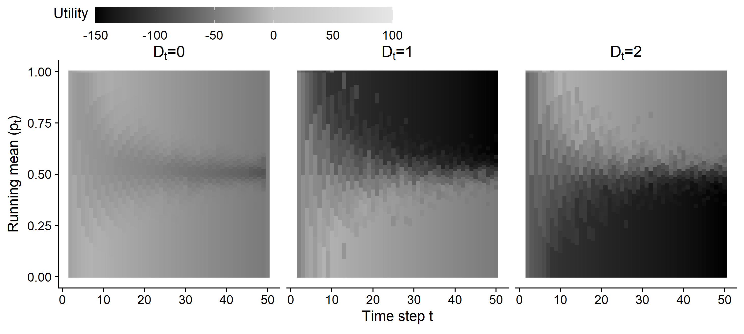
(a) BSD: expected utility estimates under constrained backward induction.

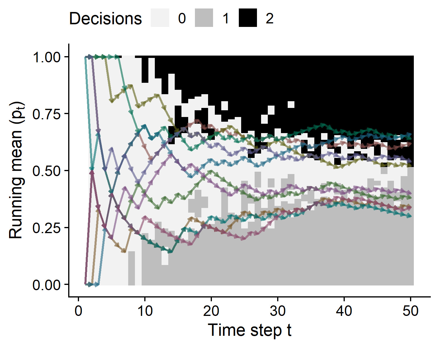
(b) BSD: optimal actions.

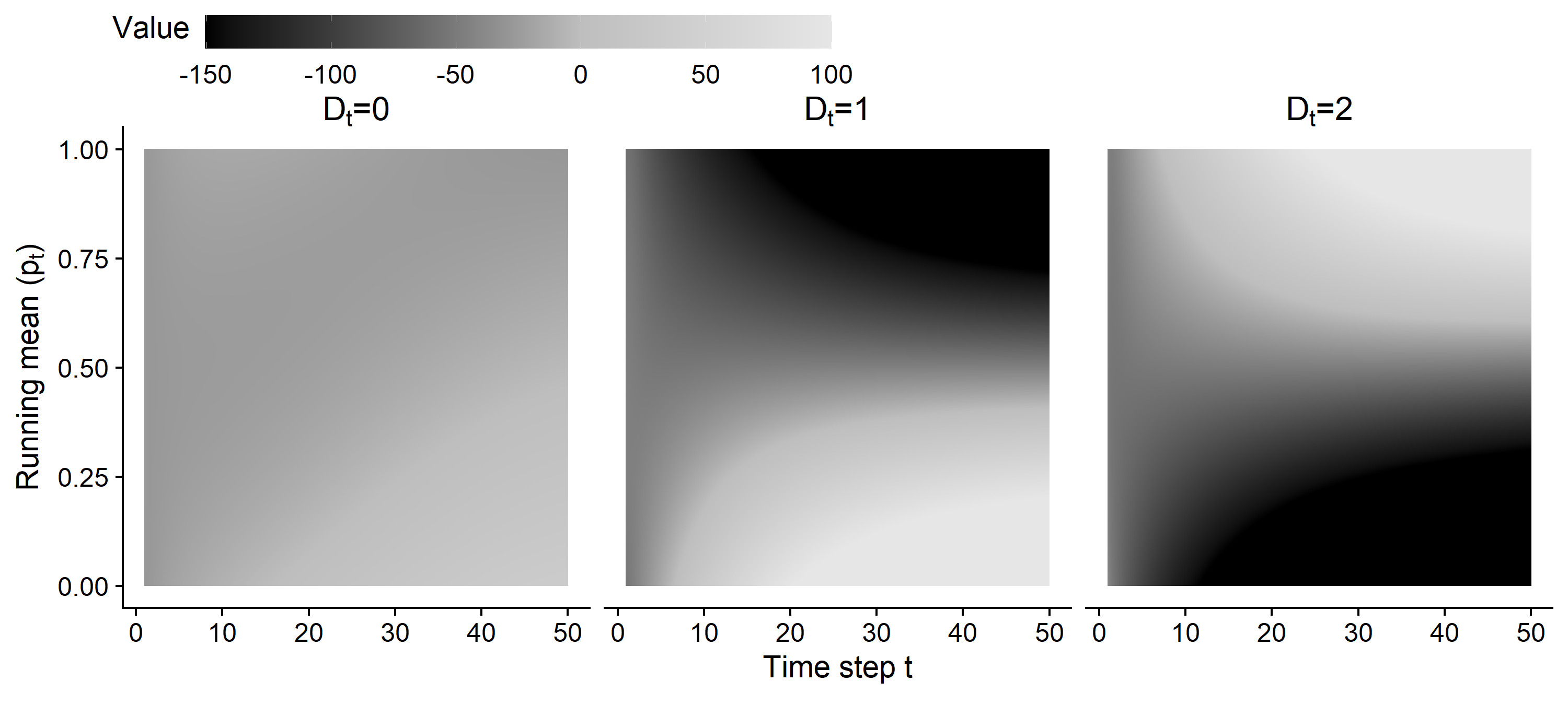
(c) RL: state-action value estimates with Q-learning

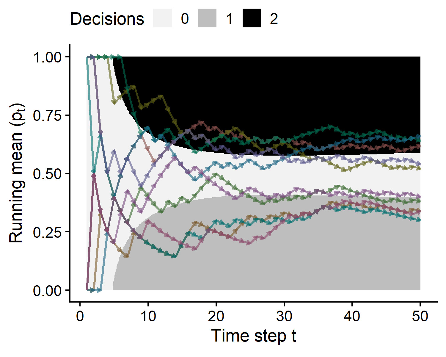
(d) RL: best actions.

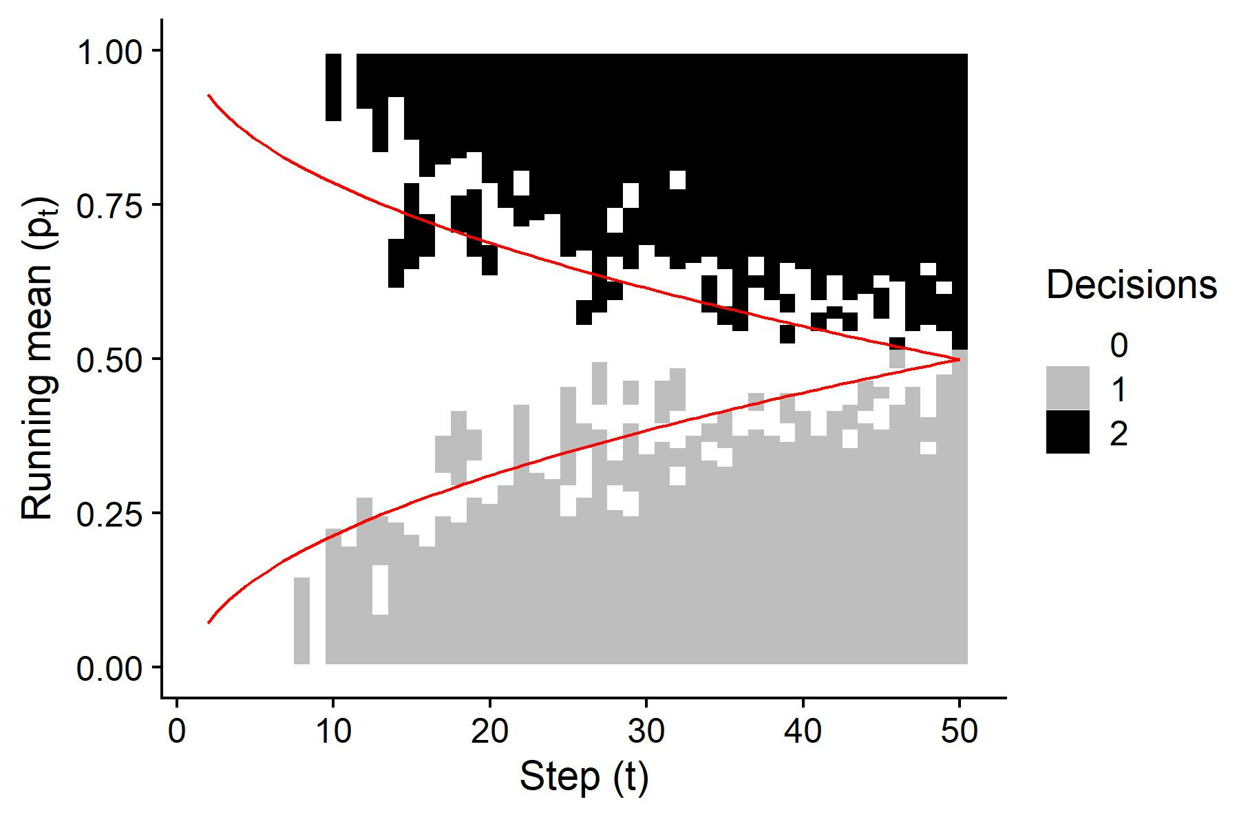
(e) BSD: parametric boundary.

(f) BSD: utility by parameter.

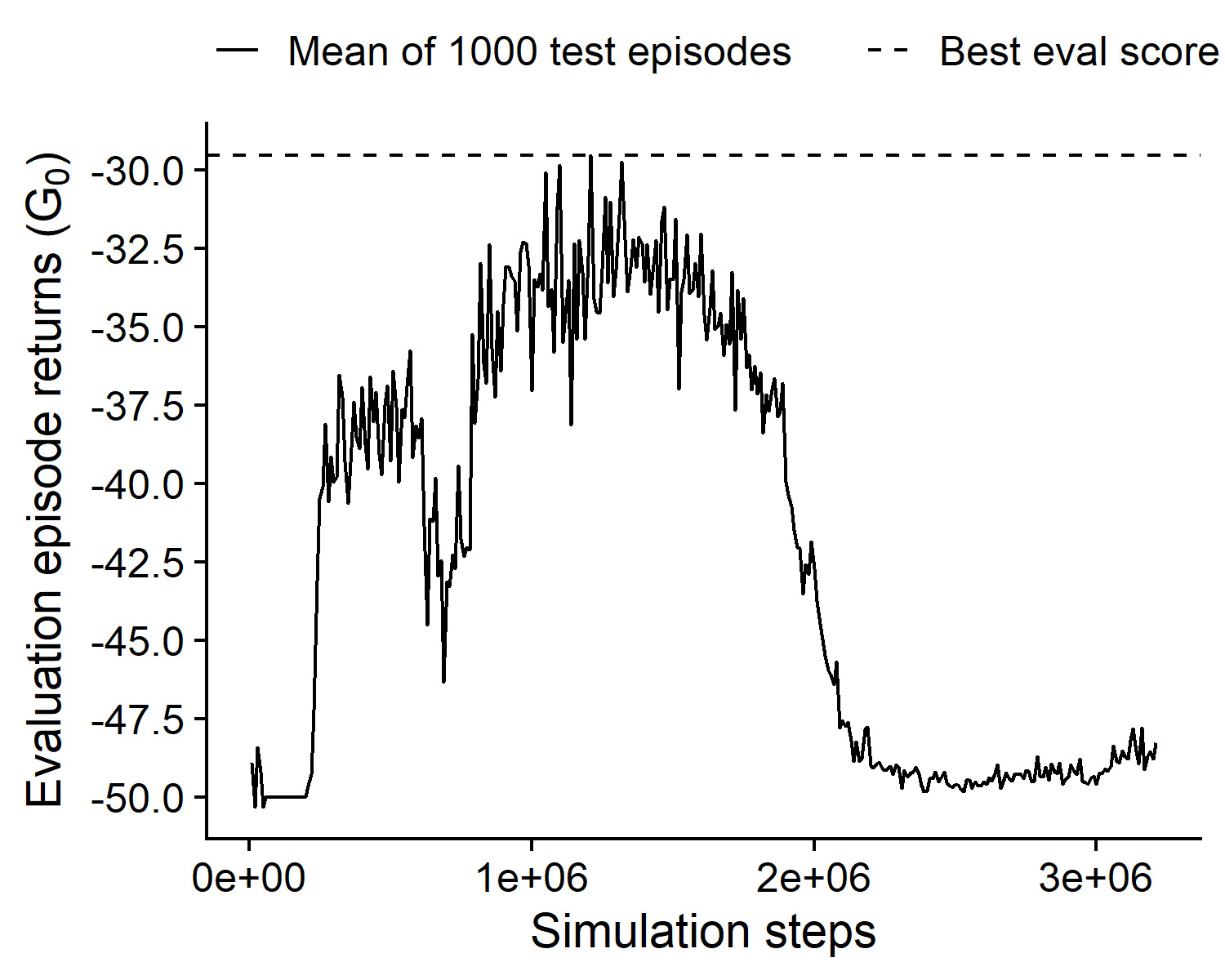
(g) RL: performance over training.

Figure 3: Example 1. Comparison of decision boundaries and fitted value functions/utilities.

3.2 Sequential design with decision boundaries

Inspection of Figure 3(b) suggests an attractive alternative algorithm. Notice the decision boundaries on $S=(t,p_{t})$ that trace a funnel with an upper boundary $\omega_{2}(t)$ separating $D^{\star}=2$ from $D^{\star}=0$, and a lower boundary $\omega_{1}(t)$ separating $D^{\star}=0$ versus $D^{\star}=1$.

Recognizing such boundaries suggests an alternative approach based on searching for optimal boundaries in a suitable family $\{\omega_{\phi,1},\omega_{\phi,2}\mid\phi\in\Phi\}$.

This approach turns the sequential decision problem of finding optimal $D^{\star}(S)$ into a non-sequential problem of finding an optimal $\phi^{\star}\in\Phi$. This method is used, for example, in Rossell et al. (2007).

In Example 1, we could use

$$\omega_{1}(t)=\frac{\phi\sqrt{t-1}}{\sqrt{T-1}},\quad\quad\omega_{2}(t)=1-\frac{(1-\phi)\sqrt{t-1}}{\sqrt{T-1}}$$

using a single tuning parameter $\phi\in(0,1)$. Both functions are linear in $\sqrt{t-1}$, and mimic the funnel shape seen in Figure 3(b). The decision rules implied by these boundaries is

$$D_{\phi}(S_{t})=\begin{cases}1&\mbox{ if }p_{t}<\omega_{1}(t)\\ 2&\mbox{ if }p_{t}>\omega_{2}(t)\\ 0&\mbox{ otherwise. }\end{cases}$$

Here, the additional subscript _ϕ in $D_{\phi}(\cdot)$ indicates that the decision follows the rule implied by decision boundaries $\omega_{j}(t;\phi)$. Note that $\omega_{1}(1)=1$ and $\omega_{2}(1)=0$, ensuring continuation at $t=1$.

For a given $\phi$, the forward simulations are used to evaluate expected utilities under the policy $D_{\phi}$. Let $T^{(m)}_{\phi}=\min\{t:\;D_{\phi}(S^{(m)}_{t}\neq 0\}$ denote the stopping time under $D_{\phi}$. Then the expected utility under policy $D_{\phi}$ is

$$U(\phi)=E\{u(S_{T_{\phi}},D_{\phi}(S_{T_{\phi}}),\theta)\}$$ (8)

where the expectation is with respect to data $Y_{T}$ and $\theta$. It is approximated as an average over all Monte Carlo simulations, stopping each simulation at $T^{(m)}_{\phi}$, as determined by the parametric decision boundaries,

$$\widehat{U}(\phi)=(1/M)\sum_{m=1}^{M}u(S^{(m)}_{T^{m}_{\phi}},D_{\phi}(S^{(m)}_{T^{m}_{\phi}}),\theta^{(m)}).$$ (9)

Optimizing $\widehat{U}(\phi)$ w.r.t. $\phi$ we find the optimal decision boundaries $\phi^{\star}=\arg\max\widehat{U}(\phi)$. As long as the nature of the sequential decision is restricted to sequential stopping, the same set of Monte Carlo simulations can be used to evaluate all $\phi$, using different truncation to evaluate $\widehat{U}(\phi)$. In general, a separate set of forward simulations for each $\phi$, or other simplifying assumptions might be required.

Figure 3(e) shows the decision boundaries for the best parameter estimated at $\phi^{\star}=0.503$ in Example 1. The estimated values for $\widehat{U}(\phi)$ are in Figure 3(f). In Figure 3(e), the boundaries using constrained backward induction are overlaid in the image for comparison. The decision boundaries trace the optimal decisions under the backward induction well. The differences in expected utility close to the decision boundary are likely very small, leaving minor variations in the decision boundary negligible.

The same approach is applied to the (slightly more complex) Example 2.

Recall the form of the summary statistics $S=(s_{\delta},\bar{\delta})$, the posterior standard deviation and mean of the ED95 effect. We use the boundaries

$$\omega_{1}(S)=-b_{1}s_{\delta}+c,\quad\quad\omega_{2}(S)=b_{2}s_{\delta}+c,$$

parameterized by $\phi=(b_{1},b_{2},c)$. The implied decision rules are

$$D_{\phi}(S)=\begin{cases}1&\mbox{if }\bar{\delta}<\omega_{1}(s_{\delta})\\ 2&\mbox{if }\bar{\delta}>\omega_{2}(s_{\delta})\\ 0&\text{otherwise}.\end{cases}$$

The results are in Figure 4(a). Again, the sequential decision problem is reduced to the optimization problem of finding the optimal $\phi$ in (9). Since now $\phi\in\Re^{3}$ the evaluation of $\widehat{U}$ requires a 3-dimensional grid. To borrow strength from Monte Carlo evaluations of (9) across neighboring grid points for $\phi$ we proceed as follows. We evaluate $\widehat{U}(\phi)$ on a coarse $10\times 10\times 10$ grid, and then fit a quadratic response surface (as a function of $\phi$) to these Monte Carlo estimates. The optimal decision $\phi^{*}$ is the maximizer of the quadratic fit. We find $\phi^{*}=(b_{1}^{*},b_{2}^{*},c^{*})=(1.572,1.200,0.515)$ Instead of evaluating $\widehat{U}$ on a regular grid over $\phi$, one could alternatively select a random number of design points (in $\phi$).

The use of parametric boundaries is closely related to the notion of function approximation and the method of policy gradients in RL, which will be described next.

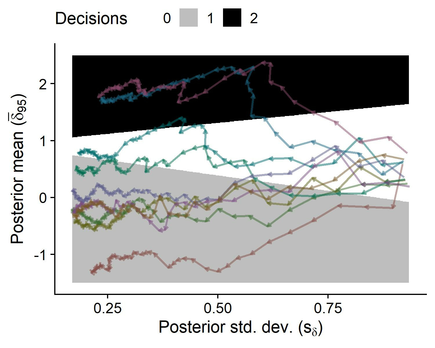
(a) BSD: parametric boundaries.

(b) RL: policy gradients

Figure 4: Optimal decisions in Example 2. Comparison of fitted decision boundaries.

4 Reinforcement learning

The basic setup in RL is usually framed in terms of Markov decision process (MDP) (Puterman, 2014). The Markov property ensures that optimal decisions depend only on the most recently observed state, enabling practicable algorithms. In this section we first describe MDPs and how a sequential design problem can be adapted to fit in this framework. Next, we discuss two algorithms, Q-learning (Watkins and Dayan, 1992) and policy gradients (Grondman et al., 2012), implemented in Example 1 and 2, respectively. Both methods are implemented using neural networks. Throughout this section, the summary statistics $S_{t}$ are referred to as states, in keeping with the common terminology in the RL literature.

(a) SDP as generic HiMDP.

(b) Resulting belief MDP.

Figure 5: Belief MDP for the SDP.

4.1 Markov decision processes and partial observability

The Markov property for a decision process is defined by the conditions

$$p(S_{t+1}\mid H_{t},D_{t})=p(S_{t+1}\mid S_{t},D_{t})\quad\quad\mbox{ and }p(R_{t}\mid H_{t},D_{t})=p(R_{t}\mid S_{t},D_{t}),$$

That is, the next state $S_{t+1}$ and the reward $R_{t}$ depend on the history only indirectly through the current state and action. When the condition holds, the decision process is called an MDP. For MDPs, the optimal policy is only a function of the latest state $S_{t}$ and not of the entire history $H_{t}$ (Puterman, 2014). Many RL algorithms assume the Markov property. However, many sequential decision problems are more naturally characterized as partially observable MDP (POMDP) that satisfy the Markov property only conditional on some $\theta$ that is generated at the beginning of each episode. Such problems have

been studied in the RL literature under the name of Hidden-Parameter MDP (HiMDP) (Doshi-Velez and Konidaris, 2016).

There is a standard – Bayesian motivated – way to cast any POMDP as an MDP using so-called belief states (Cassandra et al., 1997). Belief states are obtained by including the posterior distribution of unobserved parameters as a part of the state. With a slight abuse of notation, we may write the belief states as $S_{t}=p(\theta\mid H_{t})$. While the belief state is, in general, a function, it can often be represented as a vector when the posterior admits a finite (sufficient) summary statistic. The reward distribution can also be written in terms of such belief states as

$$p(R\mid S_{t},D_{t})=\int_{\theta}p(R\mid D_{t},\theta)\,dp(\theta\mid H_{t}).$$ (10)

See Figure 5 for a graphical representation of an HiMDP and the resulting belief MDP.

We implement this approach for Example 1. The reward is chosen to match the definition of utility. It suffices to define it in terms of $\theta$ (and let the posterior take care of the rest, using (10)). We use

$$R(d,\theta)=-c\,\mathbb{I}(d=0)-K\mathbb{I}(\theta_{d}\neq\theta,d\neq 0),$$ (11)

as in (3). Next we introduce the belief states. Recall the notation from Example 1. We have $p(\theta\mid S_{t})=\mbox{Bin}(p_{t},p_{t}(1-p_{t})/t)$. The summary statistic $S_{t}=(t,p_{t})$ is a two-dimensional representation of the belief state.

Considering Example 2, we note that the utility function (5) depends on the state $S_{t}$ only, and does not involve $\theta$. We define

$$R_{\theta}(d,S_{t})=-c_{1}\mathbb{I}(d=0)+(-c_{2}N_{\alpha,\beta}(S_{t})+K\Delta_{R}(S_{t}))\mathbb{I}(d=2).\\$$ (12)

While the reward is clearly Markovian, the transition probability is not necessarily Markovian. This is the case because in this example the posterior moments $S_{t}$ are not a sufficient statistic. In practice, however, a minor violation of the Markov assumption for the transition distribution does not seem to affect the ability to obtain good policies with standard RL techniques.

4.2 Q-learning

Q-learning (Watkins and Dayan, 1992; Clifton and Laber, 2020; Murphy, 2003) is an RL algorithm that is similar in spirit to the constrained backward induction described in Section 3.1. The starting point is Bellman optimality equation for MDPs (Bellman, 1966). Equation (6) for the optimal $D^{\star}$ and written for MDPs becomes

$$Q^{\pi_{\star}}(s,d)=\mathbb{E}\{R_{t}+\textstyle{\max_{d^{\prime}}}Q^{\pi_{\star}}(S_{t+1},d^{\prime})\mid S_{t}=s,D_{t}=d\},$$ (13)

where the expectation is with respect to $R_{t}$ and $S_{t+1}$. The optimal policy is implicitly defined as the solution to (13).

Q-learning proceeds iteratively following the fixed-point iteration principle. Let $Q^{(k)}$ be some approximation of $Q^{\star}$. We assume that a set of simulated transitions $\{(s_{t},d_{t},r_{t},s_{t+1})\}_{t=1}^{n}$ is available. This collection is used like the forward simulations in the earlier discussion. In RL it is known as the “experience replay buffer”, and can be generated using any stochastic policy. And suppose, for the moment, that the state and action spaces are finite discrete, allowing to record $Q^{(k)}$ in a table. Q-learning is defined by updating $Q^{(k)}$ as

$$Q^{(k+1)}(s_{t},d_{t})\leftarrow(1-\alpha_{k})Q^{(k)}(s_{t},d_{t})+\alpha_{k}\{r_{t}+\textstyle{\max_{d}}Q^{(k)}(s_{t+1},d)\}.$$ (14)

Note the moving average nature of the update. The procedure iterates until convergence from a stream of transitions.

Deep Q-networks (DQN) (Mnih et al., 2013) are an extension of Q-learning for continuous states. A neural network is used to represent $Q(\cdot)$. Let $\phi^{(k)}$ denote the parameters of the neural network at iteration $k$. Using simulated transitions from the buffer

DQN performs updates

$$\phi^{(k+1)}=\textstyle{\operatorname*{arg\,min}_{\phi}\sum_{t=1}^{n}}\left(r_{t}+\max_{d}Q_{\phi^{(k)}}(S_{t+1},d)-Q_{\phi}(S_{t},d_{t})\right)^{2}.$$ (15)

In practice, exact minimization is replaced by a gradient step from mini-batches, together with numerous implementation tricks (Mnih et al., 2013).

We implemented DQN in Example 1 using the Python package Stable-Baselines3 (Raffin et al., 2021). The experience replay buffer is continuously updated. The algorithm uses a random policy to produce an initial buffer and then adds experience from an $\epsilon$-greedy policy, where the current best guess for the optimal policy is chosen with probability $(1-\epsilon)$, and otherwise fully random actions are chosen with probability $\epsilon$. Figure 3(c) shows $\hat{Q}$, the estimate of $Q^{\star}$, for each state and action $d\in\{0,1,2\}$. Figure 3(d) shows the corresponding optimal actions. Overall, the results are similar to the results with constrained backward induction, but much smoother. Also, notice that the solution under DQN is usually better in terms of expected utility as shown in Figure 3(f), even in (out-of-sample) evaluation episodes. This is likely due to to the flexibility and high-dimensional nature of the neural network approximation.

The better performance of RL comes at a price. First is sample efficiency (the number of simulations required by the algorithm to yield a good policy). The best $\hat{Q}$ is obtained after 2 million sampled transitions. Data efficiency is a known problem in DQN, and in RL in general (Yu, 2018). In many real applications investigators cannot afford such a high number of simulation steps. Another limitation is training instability. In particular, Figure 3(f) illustrates a phenomenon known as catastrophic forgetting, which happens when additional training decreases the ability of the agent to perform a previously learned task (Atkinson et al., 2021). This can happen because of the instability that arises from a typical strategy of evaluating performance periodically and keeping track of the best performing policy only. Several improvements over basic DQN have been proposed, with improved performance and efficiency (Hessel et al., 2018).

4.3 Policy gradients

The approach is similar to the use of parametric boundaries discussed before. Policy gradient (PG) approaches start from a parameterization $\pi_{\bm{\phi}}$ of the policy. Again, consider a neural network (NN) with weights $\phi$. The goal of a PG method is to maximize the objective

$$\max_{\phi}J(\phi)=\mathbb{E}\{G\mid\pi_{\phi}\}.$$ (16)

This objective is the analogue to maximizing $U(\phi)$ in (9), except that here the stochastic policy $\pi_{\phi}$ is a probability distribution on decisions $S_{t}$. The main characteristic of PG methods is the use of gradient descent to solve (16).

The evaluation of gradients is based on the PG theorem (Sutton et al., 1999),

$$\nabla_{\bm{\phi}}J({\bm{\phi}})=\mathbb{E}\left\{\left[\sum_{t=1}^{T}\nabla_{\bm{\phi}}\log\pi_{\bm{\phi}}(D_{t}\mid S_{t})\right]\cdot G\mid\pi_{\phi}\right\},$$ (17)

where the total return $G$ is a function $G(\tau)$ of the entire trajectory $\tau=(S_{1},D_{1},\ldots,S_{T},D_{T})$. Using gradients, PG methods can optimize over high-dimensional parameter spaces like in neural networks. In practice, estimates of the gradient are known to have huge variance, affecting the optimization. But several implementation tricks exist that improve the stability and reduce the variance. Proximal policy optimization (PPO) (Schulman et al., 2017) incorporates many of these tricks, and is widely used as a default for PG-based methods.

The PG theorem is essentially Leibniz rule for the gradient of $J(\phi)$.

With a slight abuse of notation, write $\pi_{\bm{\phi}}(\tau)$ for the distribution of $\tau$ induced by $\pi_{\bm{\phi}}$ for the sequential decisions. Then Leibniz rule for the gradient of the integral gives

$$\nabla_{\bm{\phi}}J({\bm{\phi}})=\nabla_{\bm{\phi}}\int\pi_{\phi}(\tau)G(\tau)d\tau=\\ \int\nabla_{\bm{\phi}}\pi_{\bm{\phi}}(\tau)\cdot G(\tau)\,d\tau=\int\left(\nabla_{\bm{\phi}}\log\pi_{\bm{\phi}}(\tau)\right)\,\pi_{\bm{\phi}}(\tau)\cdot G(\tau)\,d\tau=\mathbb{E}\left\{\nabla_{\bm{\phi}}\log\pi_{\bm{\phi}}(\tau)\cdot G(\tau)\right\},$$ (18)

where the expectations are with respect to the (stochastic) policy $\pi_{\phi}$ over $\tau$. The log probability in the last expression can be written as a sum of log probabilities, yielding (17).

PPO is implemented in Example 2 using Stable-Baselines3 (Raffin et al., 2021). The results are shown in Figure 4(b). Not surprisingly, the results are similar to those obtained earlier using parametric decision boundaries. Interestingly, the figure shows that neural networks do not necessarily extrapolate well to regions with low data. This behavior is noticeable on the lower left corner of the figure, where there could be data, but where it is never observed in practice because of the early stopping implied by the boundaries.

5 Discussion

We have introduced some of the main features of RL and BSD in the context of two optimal stopping problems. In the context of these examples the two approaches are quite similar, including an almost one-to-one mapping of terminology and notation, as we attempted in Table 1. In general, however, the applicability, especially the practical use of RL is much wider. The restriction of the sequential problems to optimal stopping was only needed for easy application of the BSD solution. In contrast, RL methods are routinely used for a variety of other problems, such as robotics (Tunyasuvunakool et al., 2020) autonomous driving (Sallab et al., 2017; Wurman et al., 2022), and smart building energy management (Yu et al., 2021). The main attraction of BSD is the principled nature of the solution. One can argue from first principles that a rational agent should act as if he or she were optimizing expected utility as in (1). There is a well-defined and coherent propagation of uncertainties. This might be particularly important when the SDP and underlying model are only part of a bigger problem. Overall, we note that the perspective of one method, and corresponding algorithms can be useful for improvements in the respective other method. For example, policy gradients could readily be used to solve BSD if randomized decision rules were used. The latter is usually not considered. On the other hand, hierarchical Bayesian inference models could be used to combine multiple sources of evidence in making sequential decisions under RL, or multiple related problems could be linked in a well-defined manner in a larger encompassing model. For example, clinical trials are never carried out in isolation. Often the same department or group might run multiple trials on the same patient population for the same disease, with obvious opportunities to borrow strength.

Funding

Yunshan Duan and Peter Müller are partially funded by the NSF under grant NSF/DMS 1952679.

Conflicts of Interest

The authors report there are no competing interests to declare

Appendix

Appendix A Details in Example 2

We assume a nonlinear regression sampling model

$$Y_{t}=f(X_{t}\mid\theta)+\epsilon_{t},\;\;\;\;\epsilon_{t}\sim N(0,\sigma^{2}),$$

and the dose-response curve

$$f(X_{t}\mid\theta)=a+b\frac{X_{t}^{r}}{(q^{r}+X_{t}^{r})}$$

We fix $a,r,\sigma^{2}$, and put a normal prior on unknown parameters $\theta=(b,q)$,

$$p(\theta)=N(\theta_{0},diag(\lambda_{0})).$$

Sample size calculation

If at time $T$, the decision $D_{T}=2$ indicates stopping and a pivotal trial is conducted to test $H_{0}:\delta_{95}=0$ vs. $H_{1}:\delta_{95}>0$. We need to determine the sample size $N_{\alpha,\beta}$ for the pivotal trial that can achieve desired significance level $\alpha$ and power $(1-\beta)$, and calculate the posterior predictive probability of a significant outcome, $\Delta_{R}=\Pr(\mbox{reject $H_{0}$ in the 2nd trial}\mid H_{T})$.

Let $\bar{\delta}_{95}$ and $s_{\delta}$ denote the posterior mean and std. dev. of $\delta_{95}$. We calculate power based on $\delta_{95}=\delta^{*}$, where $\delta_{95}^{*}=\bar{\delta}_{95}-s_{\delta}$.

Now consider a test enrolling $N_{\alpha,\beta}$ patients, randomizing $N_{\alpha,\beta}/2$ at $x=0$ (placebo) and $N_{\alpha,\beta}/2$ at the estimated ED95. Assuming $var(y_{i})=1$, we need

$$N_{\alpha,\beta}\geq 4\left[(q_{\alpha}+q_{\beta})/\delta^{*}\right]^{2}$$

where $q_{\alpha}$ is the $\alpha$ right tail cutoff for the $N(0,1)$ and $\alpha=5\%$ and $(1-\beta)=80\%$ are the desired significance level and power (i.e., $\beta=0.2$).

A significant outcome at the end of the 2nd trial means data in the rejection region. Let $\overline{y}_{1},\overline{y}_{0}$ denote the sample average of $N_{\alpha,\beta}/2$ patients each to be enrolled in the two arms of the 2nd trial. Then the rejection region is

$$R=\{(\overline{y}_{1}-\overline{y}_{0})\sqrt{N_{\alpha,\beta}/4}\geq q_{\alpha}\}.$$

Let $\Phi(\cdot)$ denote the standard normal c.d.f. Then

$$\Delta_{R}=\Phi\left[\frac{\bar{\delta}\sqrt{N_{\alpha,\beta}/4}-q_{\alpha}}{\sqrt{1+\frac{N_{\alpha,\beta}}{4}s_{\delta}^{2}}}\right]$$

Posterior simulation

We can implement independent posterior simulation:

1. Generate $q\sim p(q\mid H_{t})$, using

   $$p(q\mid H_{t})\propto p(H_{t}\mid q)\cdot p(q)=\frac{p(H_{t}\mid b,q)p(b)}{p(b\mid q,H_{t})}\cdot p(q)$$

2. Then generate $b$ from the posterior conditional distribution $b\sim p(b\mid q,H_{t})$. Based on normal linear regression, the conditional posterior is a univariate normal distribution.

References

- Atkinson et al. (2021) Atkinson, C., B. McCane, L. Szymanski, and A. Robins (2021). Pseudo-rehearsal: Achieving deep reinforcement learning without catastrophic forgetting. Neurocomputing 428, 291–307.
- Bellman (1966) Bellman, R. (1966). Dynamic programming. Science 153(3731), 34–37.
- Berger (2013) Berger, J. O. (2013). Statistical decision theory and Bayesian analysis. Springer Science & Business Media.
- Berry and Ho (1988) Berry, D. A. and C.-H. Ho (1988). One-sided sequential stopping boundaries for clinical trials: A decision-theoretic approach. Biometrics 44(1), 219–227.
- Brockwell and Kadane (2003) Brockwell, A. E. and J. B. Kadane (2003). A gridding method for Bayesian sequential decision problems. Journal of Computational and Graphical Statistics 12(3), 566–584.
- Carlin et al. (1998) Carlin, B. P., J. B. Kadane, and A. E. Gelfand (1998). Approaches for optimal sequential decision analysis in clinical trials. Biometrics 54, 964–975.
- Cassandra et al. (1997) Cassandra, A., M. L. Littman, and N. L. Zhang (1997). Incremental pruning: A simple, fast, exact method for partially observable Markov decision processes. In Proceedings of the Thirteenth conference on Uncertainty in artificial intelligence, pp. 54–61.
- Christen and Nakamura (2003) Christen, J. A. and M. Nakamura (2003). Sequential stopping rules for species accumulation. Journal of Agricultural, Biological, and Environmental Statistics 8(2), 184–195.
- Clifton and Laber (2020) Clifton, J. and E. Laber (2020). Q-learning: Theory and applications. Annual Review of Statistics and Its Application 7(1), 279–301.
- DeGroot (2004) DeGroot, M. (2004). Optimal statistical decisions. New York: Wiley-Interscience.
- Doshi-Velez and Konidaris (2016) Doshi-Velez, F. and G. Konidaris (2016). Hidden parameter Markov decision processes: A semiparametric regression approach for discovering latent task parametrizations. In IJCAI: Proceedings of the Conference, Volume 2016, pp. 1432.
- Gaon and Brafman (2020) Gaon, M. and R. Brafman (2020). Reinforcement learning with non-Markovian rewards. In Thirty-fourth AAAI Conference on Artificial Intelligence.
- Grieve and Krams (2005) Grieve, A. P. and M. Krams (2005). ASTIN: A Bayesian adaptive dose–response trial in acute stroke. Clinical Trials 2(4), 340–351.
- Grondman et al. (2012) Grondman, I., L. Busoniu, G. A. Lopes, and R. Babuska (2012). A survey of actor-critic reinforcement learning: Standard and natural policy gradients. IEEE Transactions on Systems, Man, and Cybernetics, Part C (Applications and Reviews) 42(6), 1291–1307.
- Hessel et al. (2018) Hessel, M., J. Modayil, H. Van Hasselt, T. Schaul, G. Ostrovski, W. Dabney, D. Horgan, B. Piot, M. Azar, and D. Silver (2018). Rainbow: Combining improvements in deep reinforcement learning. In Thirty-second AAAI Conference on Artificial Intelligence.
- Kadane and Vlachos (2002) Kadane, J. B. and P. K. Vlachos (2002). Hybrid methods for calculating optimal few-stage sequential strategies: Data monitoring for a clinical trial. Statistics and Computing 12, 147–152.
- MacDonald et al. (2015) MacDonald, B., P. Ranjan, and H. Chipman (2015). GPfit: An R package for fitting a Gaussian process model to deterministic simulator outputs. Journal of Statistical Software 64, 1–23.
- Meibohm and Derendorf (1997) Meibohm, B. and H. Derendorf (1997). Basic concepts of pharmacokinetic/pharmacodynamic (pk/pd) modelling. International Journal of Clinical Pharmacology and Therapeutics 35(10), 401–413.
- Mnih et al. (2013) Mnih, V., K. Kavukcuoglu, D. Silver, A. Graves, I. Antonoglou, D. Wierstra, and M. Riedmiller (2013). Playing Atari with deep reinforcement learning. arXiv preprint 1312.5602.
- Müller et al. (2007) Müller, P., D. A. Berry, A. P. Grieve, M. Smith, and M. Krams (2007). Simulation-based sequential Bayesian design. Journal of Statistical Planning and Inference 137(10), 3140–3150.
- Murphy (2003) Murphy, S. A. (2003). Optimal dynamic treatment regimes. Journal of the Royal Statistical Society: Series B (Statistical Methodology) 65(2), 331–355.
- Murphy et al. (2007) Murphy, S. A., D. W. Oslin, A. J. Rush, and J. Zhu (2007). Methodological challenges in constructing effective treatment sequences for chronic psychiatric disorders. Neuropsychopharmacology 32(2), 257–262.
- Parmigiani and Inoue (2009) Parmigiani, G. and L. Inoue (2009). Decision Theory: Principles and Approaches. Wiley.
- Puterman (2014) Puterman, M. L. (2014). Markov decision processes: Discrete stochastic dynamic programming. John Wiley & Sons.
- Raffin et al. (2021) Raffin, A., A. Hill, A. Gleave, A. Kanervisto, M. Ernestus, and N. Dormann (2021). Stable-baselines3: Reliable reinforcement learning implementations. Journal of Machine Learning Research 22(268), 1–8.
- Robins (1997) Robins, J. M. (1997). Causal inference from complex longitudinal data. In Latent variable modeling and applications to causality, pp. 69–117. Springer.
- Rossell et al. (2007) Rossell, D., P. Müller, and G. Rosner (2007). Screening designs for drug development. Biostatistics 8, 595–608.
- Sallab et al. (2017) Sallab, A. E., M. Abdou, E. Perot, and S. Yogamani (2017). Deep reinforcement learning framework for autonomous driving. Electronic Imaging 2017(19), 70–76.
- Schulman et al. (2017) Schulman, J., F. Wolski, P. Dhariwal, A. Radford, and O. Klimov (2017). Proximal policy optimization algorithms. arXiv preprint 1707.06347.
- Shen and Huan (2021) Shen, W. and X. Huan (2021). Bayesian sequential optimal experimental design for nonlinear models using policy gradient reinforcement learning. arXiv preprint 2110.15335.
- Silver et al. (2018) Silver, D., T. Hubert, J. Schrittwieser, I. Antonoglou, M. Lai, A. Guez, M. Lanctot, L. Sifre, D. Kumaran, T. Graepel, et al. (2018). A general reinforcement learning algorithm that masters chess, shogi, and go through self-play. Science 362(6419), 1140–1144.
- Silver et al. (2014) Silver, D., G. Lever, N. Heess, T. Degris, D. Wierstra, and M. Riedmiller (2014). Deterministic policy gradient algorithms. In Proceedings of the 31st International Conference on International Conference on Machine Learning, pp. 387–395.
- Sutton and Barto (2018) Sutton, R. S. and A. G. Barto (2018). Reinforcement learning: An introduction. MIT Press 5, 31.
- Sutton et al. (1999) Sutton, R. S., D. McAllester, S. Singh, and Y. Mansour (1999). Policy gradient methods for reinforcement learning with function approximation. In S. Solla, T. Leen, and K. Müller (Eds.), Advances in Neural Information Processing Systems, Volume 12.
- Tunyasuvunakool et al. (2020) Tunyasuvunakool, S., A. Muldal, Y. Doron, S. Liu, S. Bohez, J. Merel, T. Erez, T. Lillicrap, N. Heess, and Y. Tassa (2020). dm_control: Software and tasks for continuous control. Software Impacts 6, 100022.
- Watkins and Dayan (1992) Watkins, C. J. and P. Dayan (1992). Q-learning. Machine learning 8(3-4), 279–292.
- Wurman et al. (2022) Wurman, P. R., S. Barrett, K. Kawamoto, J. MacGlashan, K. Subramanian, T. J. Walsh, R. Capobianco, A. Devlic, F. Eckert, F. Fuchs, et al. (2022). Outracing champion gran turismo drivers with deep reinforcement learning. Nature 602(7896), 223–228.
- Yu et al. (2021) Yu, L., S. Qin, M. Zhang, C. Shen, T. Jiang, and X. Guan (2021). A review of deep reinforcement learning for smart building energy management. IEEE Internet of Things Journal 8, 12046–12063.
- Yu (2018) Yu, Y. (2018). Towards sample efficient reinforcement learning. In Proceedings of the Twenty-Seventh International Joint Conference on Artificial Intelligence.
- Zhao et al. (2009) Zhao, Y., M. R. Kosorok, and D. Zeng (2009). Reinforcement learning design for cancer clinical trials. Statistics in Medicine 28(26), 3294–3315.